Gradient Weighted Superpixels for Interpretability in CNNs

Abstract

As Convolutional Neural Networks embed themselves into our everyday lives, the need for them to be interpretable increases. However, there is often a trade-off between methods that are efficient to compute but produce an explanation that is difficult to interpret, and those that are slow to compute but provide a more interpretable result. This is particularly challenging in problem spaces that require a large input volume, especially video which combines both spatial and temporal dimensions. In this work we introduce the idea of scoring superpixels through the use of gradient based pixel scoring techniques. We show qualitatively and quantitatively that this is able to approximate LIME, in a fraction of the time. We investigate our techniques using both image classification, and action recognition networks on large scale datasets (ImageNet and Kinetics-400 respectively).

1 Introduction

Convolutional Neural Networks (CNNs) are often described as black boxes due to the difficulty in explaining how they reach their final output for a given task. Consequently a number of techniques have been developed to aid in the process of explainability. These techniques range from the scoring of individual pixels to reflect their impact on the networks decision making, to the scoring of larger regions of the image. Scoring larger regions allows for the results to be more easily interpreted.

A popular technique for explaining images is LIME [Ribeiro et al.(2016)Ribeiro, Singh, and Guestrin]. This uses superpixels, contiguous regions for visualisation, allowing a level of interpretability that may not be present in individual pixel scoring. However, this increased interpretability comes at a cost. The LIME technique relies on perturbing the input image and repeatedly passing it to the network to build an understanding of how important each superpixel region is to the final classification. This requires multiple perturbed images to be passed through the network, by default $1000$ in the released code. Having such a computationally intensive method for ranking regions of an input is problematic when we have a need for real-time generation of visualisations, or where the input is more complex than a 2D image, i.e. a 3D spatio-temporal input such as video.

Interpretability of networks is an important area of research, particularly as techniques come under both increased scrutiny and an expectation they will be able to give an explanation for their decision (i.e. with the recent EU GDPR coming into effect). Having techniques that are efficient to compute as well as being easy to interpret are therefore crucial. As interpretability techniques have improved, they have had a tendency to become more complicated to compute. For example a number of techniques require multiple passes through the network to explain a single input  [Fong and Vedaldi(2017), Ribeiro et al.(2016)Ribeiro, Singh, and Guestrin, Zeiler and Fergus(2014), Sundararajan et al.(2017)Sundararajan, Taly, and Yan]. We propose a method to approximate the results generated by LIME using using a much less time consuming method.

In this paper we propose a method for weighting superpixels through the use of aggregated pixel values, achievable in a single forward and backward pass of the network. We show that our technique is comparable to LIME for a modest number of passes through the network. We also show how this technique can be extended for use in spatiotemporal inputs, allowing a novel method of explaining action recognition networks to be developed.

2 Related Work

A number of works have previously attempted to explain how and why a network has made its decision based on the input space. Initially this work was based on back propagating the gradients from the output to the input pixels  [Simonyan et al.(2013)Simonyan, Vedaldi, and Zisserman, Zeiler and Fergus(2014)]. These techniques were built upon further with the use of guided backpropagation [Springenberg et al.(2014)Springenberg, Dosovitskiy, Brox, and Riedmiller], then further expanded by combining the gradient with the activations during backpropagation in works such as Layer-wise Relevance Propagation (LRP) [Bach et al.(2015)Bach, Binder, Montavon, Klauschen, Müller, and Samek], Deep Taylor  [Montavon et al.(2017)Montavon, Lapuschkin, Binder, Samek, and Müller], and Excitation Backprop [Zhang et al.(2018)Zhang, Bargal, Lin, Brandt, Shen, and Sclaroff]. Integrated Gradients [Shrikumar et al.(2017)Shrikumar, Greenside, and Kundaje] propose that instead of using a single input, it is better to have a range of scaled inputs (i.e. from zeros to the original input values) and integrate the corresponding gradients. This work also introduced gradient $\odot$ input as a visualisation method. Class Activation Maps [Zhou et al.(2016)Zhou, Khosla, A., Oliva, and Torralba] (CAMs) allow networks with a Global Average Pooling (GAP) layer to localise discriminative regions within the input space. This was generalised in Grad-CAM [Selvaraju et al.(2017)Selvaraju, Cogswell, Das, Vedantam, Parikh, and Batra] to allow networks without a GAP layer to produce class activation maps through the visualisation of the final activation map weighted with the mean gradients. The technique was adapted with Grad-CAM++ [Chattopadhyay et al.(2018)Chattopadhyay, Sarkar, Howlader, and Balasubramanian] which aimed to improve Grad-CAMs localisation ability.

Methods have been developed that treat the network as a black box and perturb the image space to discover how the network makes it decision. An early example of this was occlusion maps [Zeiler and Fergus(2014)], which iterates a blank patch over the input space and stores the softmax score for each position. As the blank patch moves over important features, the softmax score should drop allowing a visualisation to be built showing which pixels are important to the network. A more recent example of a black box technique is LIME [Ribeiro et al.(2016)Ribeiro, Singh, and Guestrin] which segments the input space using superpixels before perturbing them by turning superpixels on or off (i.e. setting the superpixel to the median value of the input image). A linear regression model is then trained on the perturbations and corresponding scores. By interpreting this local model, superpixels can be selected that indicate the important regions of the image. This idea of perturbing the input space was investigated further in the work by Fong et al [Fong and Vedaldi(2017)] which again treats the network as a black box but attempts to learn a mask that maximally suppresses the softmax score for the given input.

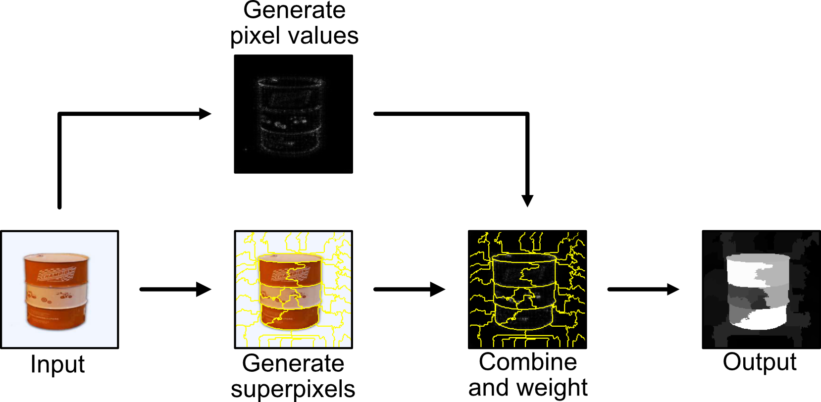
Figure 1: A simple overview of our proposed method.

3 Proposal

Our proposed method is an alternative to the time consuming method used by LIME. Rather than generating a number of perturbed images and seeing how the network reacts, we suggest generating the superpixels in the same way but then weighting each one using the values from a pixel scoring method. Previous interpretability techniques have produced saliency maps based on backpropagating gradients back to the initial input to indicate which pixels are important and which are not. With a score for each pixel we suggest using the values contained within each superpixel to provide an overall weight. An overview of the proposed technique can be found in Figure 1. In this way we are able to approximate LIME [Ribeiro et al.(2016)Ribeiro, Singh, and Guestrin] with its interpretable superpixels with a reduced computational footprint.

We have specifically chosen pixel scoring methods that require at most a single forward and backward pass through the network. We investigate the following techniques for producing pixel scores, an example of each are shown in Figure  2:

Vanilla [Simonyan et al.(2013)Simonyan, Vedaldi, and Zisserman]

Pixel scores produced by back propagating gradients from the softmax layer (for a given class) to the input.

Guided Vanilla [Springenberg et al.(2014)Springenberg, Dosovitskiy, Brox, and Riedmiller]

As with vanilla backpropagation except only positive gradients are backpropagated.

Input$\odot$Gradient [Shrikumar et al.(2017)Shrikumar, Greenside, and Kundaje]

The product of the input image and the vanilla backpropagation.

ReLU Activation

The rectified activation map produced by the final convolution layer. This is resized to match the input dimensions.

Grad-CAM [Selvaraju et al.(2017)Selvaraju, Cogswell, Das, Vedantam, Parikh, and Batra]

The weighted rectified activation map produced by the final convolution layer. Here the weights are produced from the mean of the gradients at the final convolution layer.

Guided Grad-CAM [Selvaraju et al.(2017)Selvaraju, Cogswell, Das, Vedantam, Parikh, and Batra]

The product of guided backpropagation and Grad-CAM.

Grad-CAM++ [Chattopadhyay et al.(2018)Chattopadhyay, Sarkar, Howlader, and Balasubramanian]

A variant of Grad-CAM that uses a weighted combination of the positive partial derivatives to inform the weights.

Act$\odot$Grad-CAM

The weighted rectified activation map produced by the final convolution layer. Here the weights are produced from the mean of the product of the activations and gradients at the final convolution layer.

Guided Act$\odot$Grad-CAM

The product of guided backpropagation and Act$\odot$Grad-CAM.

VGG16
Input	Vanilla	Guided Vanilla	I$\odot$G	Activation
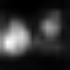
Grad-CAM	Guided Grad	Grad-CAM++	A$\odot$G-CAM	Guided A$\odot$G

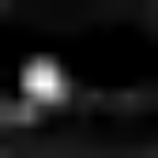
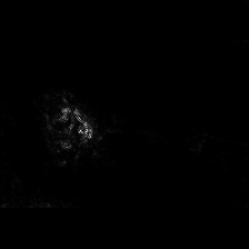
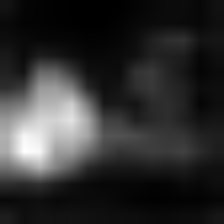
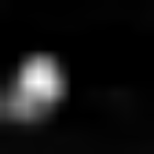
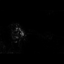
Figure 2: Examples of the nine methods investigated using PyTorch’s [Paszke et al.(2017)Paszke, Gross, Chintala, Chanan, Yang, DeVito, Lin, Desmaison, Antiga, and Lerer] pretrained VGG16 network. The input image is classified as a dog suggesting that all the techniques tried are able to correctly locate and explain the dog region in some way.

For each method we sum the absolute values of each pixel located within its respective superpixel to generate that superpixel’s weight. Other methods of distilling the pixel values into superpixel scores were investigated, however the sum of absolute values was found to be superior.

3.1 Generating Explanations

A benefit of using LIME to explain images is that it allows the superpixels that contribute to a given class to be highlighted. By visualising the superpixels that contribute to that class, a greater degree of trust can be gained in the network [Ribeiro et al.(2016)Ribeiro, Singh, and Guestrin]. To allow our method to explain different classes, we must alter the class that we backpropagate from. This method works for all pixel scoring techniques except for the raw activations. An example is shown in Figure 3.

Input	Superpixels	Dog	Cat

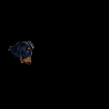
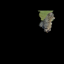
Figure 3: An example of explanations generated for the classes “Bernese mountain dog” and “Tabby”. Here we visualise the most important superpixel for each class.

3.2 Extension to Video

An interesting extension to this technique is in its use for networks that require temporal inputs. Typically these networks take longer to process a block of temporal information compared to a single image, this amplifies the time issues faced by LIME. Temporal networks are often difficult to visualise using techniques developed for image networks. For example, with techniques that derive their understanding of the network from the final convolution layer (i.e. CAM or Grad-CAM), not only do they have to be resized spatially as with an image, but also temporally. For example, in the C3D network [Tran et al.(2015)Tran, Bourdev, Fergus, Torresani, and Paluri] the initial $16$ frames are compressed to $2$ by the final convolution layer.

We propose using a segmentation technique that accommodates 3D volumes to allow our segments to extend through time. Using the pixel scores from the previously discussed techniques, we weight our 3D segments in the same manner as images. An example of our technique is shown in Figure 4.

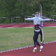
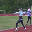
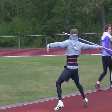
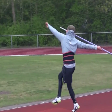
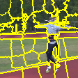
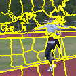
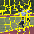
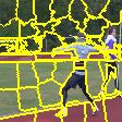
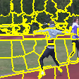
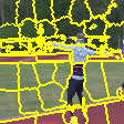
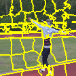
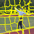
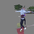
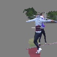
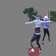
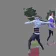
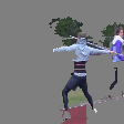
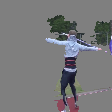
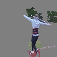
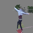
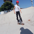
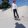
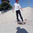
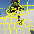
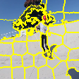
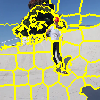
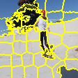
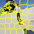
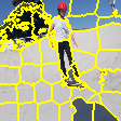
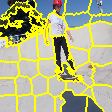
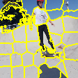
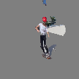
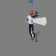
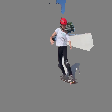
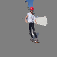
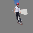
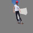
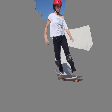
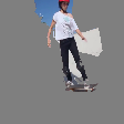
Figure 4: Example of technique applied to videos for the classes “Javelin Throw” and “Skateboarding” respectively. Showing alternating frames from a 16 frame input, the generated superpixels and the top 5 superpixels.

4 Experiments

We baseline our proposed technique against both LIME and the random ranking of superpixels. As we are aiming to find an efficient alternative to LIME we perform a number of baseline experiments with a differing number of sample inputs, i.e. the number of perturbed images fed into the network for each image. This allows us to understand if and where a trade off point between using our proposed technique and LIME exists.

All work is implemented in PyTorch [Paszke et al.(2017)Paszke, Gross, Chintala, Chanan, Yang, DeVito, Lin, Desmaison, Antiga, and Lerer]. For image classification models we use the pretrained VGG16 [Simonyan and Zisserman(2015)] and ResNet50 [He et al.(2016)He, Zhang, Ren, and Sun] networks with ImageNet. For action recognition we use our own implementation of C3D loaded with weights for the Kinetics-400 dataset [Kay et al.(2017)Kay, Carreira, Simonyan, Zhang, Hillier, Vijayanarasimhan, Viola, Green, Back, Natsev, et al., Carreira and Zisserman(2017)] released by the authors alongside their R(2+1)D model [Tran et al.(2018)Tran, Wang, Torresani, Ray, LeCun, and Paluri]. Whilst C3D is not state of the art it still uses a similar input size (i.e. 112$\times$112$\times$16) as more more recent models. Generation of superpixels is achieved using QuickShift [Vedaldi and Soatto(2008)] for image classification task and SLIC  [Achanta et al.(2012)Achanta, Shaji, Smith, Lucchi, Fua, and Süsstrunk] for action recognition tasks. We seed the method for generating superpixels to ensure the generated superpixels are identical across all experiments.

Input	Superpix	Guided	G-CAM	AG-CAM	LIME50	LIME75	LIME100	LIME5000

Figure 5: Examples of three of the better performing weighting methods compared to LIME with 50, 75, 100, and 5000 samples. Here we use 5000 samples to show how LIME with a much larger number of samples than would normally be practical. Here, guided, G-CAM, and AG-CAM refer to guided-backpropagation, Grad-CAM and Act$\odot$Grad-CAM respectively. These results are generated using VGG16 with ImageNet.

4.1 Superpixel Removal

We propose experiments to measure how well a technique ranks superpixels. To understand how accurately the superpixels are ranked we suggest iteratively removing the highest ranked superpixels from the image and seeing how many can be removed before the network no longer classifies the image correctly. The better any technique is at ranking the superpixels the fewer we should be able to remove before the image is misclassified. Alternatively, we also propose iteratively removing the lowest ranked superpixels until the image is misclassified. The more superpixels that can be removed shows how accurate a technique is at identifying areas of low importance. These results are reported as the average percentage of superpixels removed over the ImageNet validation set. An example of three of the better performing weighting methods compared to LIME is shown in Figure 5. Results for this experiment are found in Table 1.

		VGG16			ResNet50			C3D
Method		Worst	Best		Worst	Best		Worst	Best
Random		34.48%	34.50%		40.45%	40.47%		25.49%	25.66%
LIME 50		60.78%	13.07%		68.83%	15.77%		42.44%	12.14%
LIME 75		64.02%	11.16%		71.69%	13.54%		45.25%	10.30%
LIME 100		66.15%	9.87%		73.59%	12.35%		47.93%	9.12%
LIME 500		74.79%	7.20%		79.84%	9.20%		59.97%	5.92%
LIME 1000		76.16%	6.94%		80.85%	8.81%		63.20%	5.54%
Vanilla		61.50%	14.21%		66.18%	19.36%		45.91%	14.95%
Guided Vanilla		66.60%	11.40%		72.01%	14.85%		49.96%	11.92%
Input$\odot$Gradient		59.38%	16.53%		64.14%	21.57%		43.90%	16.29%
Grad-CAM		65.83%	12.24%		71.84%	14.75%		48.49%	14.69%
Guided Grad-CAM		66.31%	13.09%		74.35%	14.19%		51.19%	12.53%
Grad-CAM++		64.89%	12.25%		69.91%	15.39%		47.95%	14.75%
Act$\odot$Grad-CAM		67.28%	11.31%		70.54%	15.09%		47.85%	15.50%
Guided Act$\odot$Grad-CAM		67.30%	11.68%		73.51%	14.33%		50.99%	13.07%
ReLU Activation		63.70%	12.64%		66.26%	17.70%		42.32%	20.86%

Table 1: Results for superpixel removal where “Best” refers to the removal of the highest ranked superpixels first and “Worst” is the removal of the lowest ranked superpixels first. For “Best”, a low score is preferable, and “Worst” a high score is preferable.

These results suggest that all the implemented gradient techniques offer some ability to correctly weight the superpixels in a similar way to LIME. All techniques investigated, beat the random ranking of superpixels. A number of techniques in particular perform well, notably Act$\odot$Grad-CAM for VGG-16 and Guided Grad-CAM for ResNet50. Conversely with the C3D network we find that guided backprop performs the best. This is presumably due to the previously discussed problems with expanding CAMS back to the original temporal dimension. Overall the most consistent method for all networks is guided backpropagation which is only $-0.09\%$ from the best performing VGG16 method, and $-0.66\%$ from ResNet50’s best performing method. Interestingly, our proposed technique is consistently better at ranking the worst performing superpixels. For each model we are able to find a weighting method that beats LIME with $100$ samples.

4.2 Top $k$ Comparison

Besides comparing how well our proposed technique compares at overall ranking of superpixels, we also propose an experiment to compare how well we can identify the most important superpixel. We use LIME with 1000 samples as our baseline. This is important as, whilst the previous experiment shows how well our proposed method does in general, the robustness of networks to pixel removal may distort these results when taken as a whole. In contrast this experiment allows us to ascertain the proposed methods precision at the superpixel level. For a given unseen input, if the superpixel ranked as the most important is the same as that identified in the top $k$ ranked superpixels using the baseline technique, we call it correct. Performing this for all inputs in the validation set gives us an accuracy for each method. We also compare against LIME with smaller samples. Results are shown in Table 2.

		$k=1$				$k=5$
Method		VGG16	ResNet50	C3D		VGG16	ResNet50	C3D
LIME 50		43.71%	49.27%	23.93%		69.98%	76.44%	47.63%
LIME 75		51.07%	57.34%	30.40%		77.18%	83.61%	55.92%
LIME 100		56.27%	62.59%	35.79%		81.53%	87.97%	61.53%
LIME 500		76.82%	80.88%	61.85%		95.23%	97.62%	87.33%
Vanilla		32.27%	27.96%	24.04%		65.30%	60.34%	52.47%
Guided Vanilla		44.95%	44.48%	33.24%		78.58%	78.09%	64.05%
Input$\odot$Gradient		26.17%	23.16%	18.75%		57.09%	53.42%	45.35%
Grad-CAM		41.29%	36.75%	22.88%		78.36%	74.62%	52.42%
Guided Grad-CAM		40.36%	48.71%	31.97%		77.12%	82.93%	63.55%
Grad-CAM++		39.43%	34.37%	20.47%		75.27%	71.16%	45.37%
Act$\odot$Grad-CAM		43.55%	34.84%	22.31%		80.09%	72.22%	51.41%
Guided Act$\odot$Grad-CAM		43.32%	47.35%	31.33%		78.99%	81.35%	63.06%
ReLU Activation		37.15%	27.90%	5.53%		72.09%	61.62%	17.94%

Table 2: Top k results compared to LIME 1000

In these results we can see that again our proposed technique of weighting the segments is comparable to LIME for around 50 to 75 samples. When trying to find the most import superpixel chosen by LIME with $1000$ samples within the top $5$ predictions both VGG16 and C3D results are closer to LIME with $100$ samples.

4.3 Time Comparison

We position our proposed method as a fast alternative to LIME, therefore we perform a timing experiment to ascertain how long it takes on average to generate the superpixel scores for a number of the better performing methods from our superpixel removal experiments, and for LIME with various number of samples. For each proposed method we average the time taken to generate the scores for the images in the validation set of either ImageNet or Kinetics-400 depending on the network. We do not include the generation of the superpixels within the timings as this is common to both techniques. For LIME we use the implementation released by the authors and follow their guidance on using it with PyTorch. The results for each of the networks can be found in Figure 6.

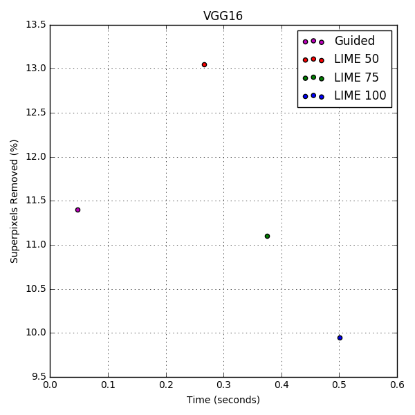
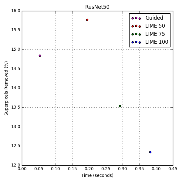
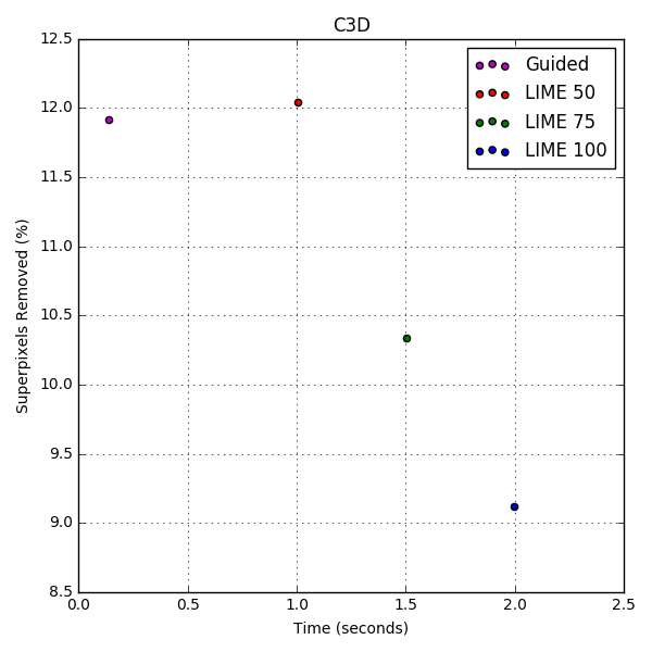
Figure 6: Results for the average time taken for weighting segments with guided backpropagation compared to LIME using 50, 75 and 100 samples.

From the results in Table 2 it is clear to see that the more samples used with LIME the better the ability to accurately score the superpixels is. However, that comes at the cost of efficiency. Our proposed method is able to approximate LIME between $50$ and $75$ samples with only a single pass through the network, this results in a much more efficient visualisation time. Of particular note is the C3D network where our method is able to visualise a $16$ frame temporal volume in $0.13$ seconds compared to $1.0$ seconds and $1.5$ seconds for LIME with 50 and 75 samples respectively.

5 Conclusion

In this paper we have introduced a novel method for weighting superpixels using easy and efficient to obtain pixel values generated with standard visualisation techniques. We have performed experiments to discover which of these methods provide the best performance in use and shown how similar results to LIME can be achieved in a time efficient manner. We have extended the technique to action recognition networks and shown how it can be applied to offer insight into networks using a temporal volume as an input.

6 Future Work

Going forward there are a number of methods  [Montavon et al.(2017)Montavon, Lapuschkin, Binder, Samek, and Müller, Zhang et al.(2018)Zhang, Bargal, Lin, Brandt, Shen, and Sclaroff, Shrikumar et al.(2017)Shrikumar, Greenside, and Kundaje] for generating pixel values that would be useful to explore. We would also like to experiment with varying the number of superpixels generated as the more superpixels present in an image, the finer grained the explanation becomes, but the longer it takes for LIME to compute. Finally, expanding the methods use in action recognition networks could prove fruitful.

7 Acknowledgements

This work is generously funded by BAE Systems and the EPSRC via iCASE award 1852482.

References

- [Achanta et al.(2012)Achanta, Shaji, Smith, Lucchi, Fua, and Süsstrunk] Radhakrishna Achanta, Appu Shaji, Kevin Smith, Aurelien Lucchi, Pascal Fua, and Sabine Süsstrunk. Slic superpixels compared to state-of-the-art superpixel methods. IEEE transactions on pattern analysis and machine intelligence, 34(11):2274–2282, 2012.
- [Bach et al.(2015)Bach, Binder, Montavon, Klauschen, Müller, and Samek] Sebastian Bach, Alexander Binder, Grégoire Montavon, Frederick Klauschen, Klaus-Robert Müller, and Wojciech Samek. On pixel-wise explanations for non-linear classifier decisions by layer-wise relevance propagation. PLoS ONE, 10(7):e0130140, 07 2015. 10.1371/journal.pone.0130140. URL http://dx.doi.org/10.1371%2Fjournal.pone.0130140.
- [Carreira and Zisserman(2017)] Joao Carreira and Andrew Zisserman. Quo vadis, action recognition? A new model and the kinetics dataset. In proceedings of the IEEE Conference on Computer Vision and Pattern Recognition, pages 6299–6308, 2017.
- [Chattopadhyay et al.(2018)Chattopadhyay, Sarkar, Howlader, and Balasubramanian] Aditya Chattopadhyay, Anirban Sarkar, Prantik Howlader, and Vineeth N. Balasubramanian. Grad-cam++: Generalized gradient-based visual explanations for deep convolutional networks. In 2018 IEEE Winter Conference on Applications of Computer Vision, WACV 2018, Lake Tahoe, NV, USA, March 12-15, 2018, pages 839–847, 2018. 10.1109/WACV.2018.00097. URL https://doi.org/10.1109/WACV.2018.00097.
- [Fong and Vedaldi(2017)] Ruth C Fong and Andrea Vedaldi. Interpretable explanations of black boxes by meaningful perturbation. In The IEEE International Conference on Computer Vision (ICCV), Oct 2017.
- [He et al.(2016)He, Zhang, Ren, and Sun] Kaiming He, Xiangyu Zhang, Shaoqing Ren, and Jian Sun. Deep residual learning for image recognition. In The IEEE Conference on Computer Vision and Pattern Recognition (CVPR), June 2016.
- [Kay et al.(2017)Kay, Carreira, Simonyan, Zhang, Hillier, Vijayanarasimhan, Viola, Green, Back, Natsev, et al.] Will Kay, Joao Carreira, Karen Simonyan, Brian Zhang, Chloe Hillier, Sudheendra Vijayanarasimhan, Fabio Viola, Tim Green, Trevor Back, Paul Natsev, et al. The kinetics human action video dataset. arXiv preprint arXiv:1705.06950, 2017.
- [Montavon et al.(2017)Montavon, Lapuschkin, Binder, Samek, and Müller] Grégoire Montavon, Sebastian Lapuschkin, Alexander Binder, Wojciech Samek, and Klaus-Robert Müller. Explaining nonlinear classification decisions with deep taylor decomposition. Pattern Recognition, 65:211–222, 2017.
- [Paszke et al.(2017)Paszke, Gross, Chintala, Chanan, Yang, DeVito, Lin, Desmaison, Antiga, and Lerer] Adam Paszke, Sam Gross, Soumith Chintala, Gregory Chanan, Edward Yang, Zachary DeVito, Zeming Lin, Alban Desmaison, Luca Antiga, and Adam Lerer. Automatic differentiation in pytorch. In NIPS-W, 2017.
- [Ribeiro et al.(2016)Ribeiro, Singh, and Guestrin] Marco Tulio Ribeiro, Sameer Singh, and Carlos Guestrin. "Why should I trust you?": Explaining the predictions of any classifier. In Proceedings of the 22nd ACM SIGKDD International Conference on Knowledge Discovery and Data Mining, San Francisco, CA, USA, August 13-17, 2016, pages 1135–1144, 2016.
- [Selvaraju et al.(2017)Selvaraju, Cogswell, Das, Vedantam, Parikh, and Batra] Ramprasaath R. Selvaraju, Michael Cogswell, Abhishek Das, Ramakrishna Vedantam, Devi Parikh, and Dhruv Batra. Grad-CAM: Visual explanations from deep networks via gradient-based localization. In The IEEE International Conference on Computer Vision (ICCV), Oct 2017.
- [Shrikumar et al.(2017)Shrikumar, Greenside, and Kundaje] Avanti Shrikumar, Peyton Greenside, and Anshul Kundaje. Learning important features through propagating activation differences. In Doina Precup and Yee Whye Teh, editors, Proceedings of the 34th International Conference on Machine Learning, volume 70 of Proceedings of Machine Learning Research, pages 3145–3153, International Convention Centre, Sydney, Australia, 06–11 Aug 2017. PMLR. URL http://proceedings.mlr.press/v70/shrikumar17a.html.
- [Simonyan and Zisserman(2015)] K. Simonyan and A. Zisserman. Very deep convolutional networks for large-scale image recognition. In International Conference on Learning Representations, 2015.
- [Simonyan et al.(2013)Simonyan, Vedaldi, and Zisserman] Karen Simonyan, Andrea Vedaldi, and Andrew Zisserman. Deep inside convolutional networks: Visualising image classification models and saliency maps. arXiv preprint arXiv:1312.6034, 2013.
- [Springenberg et al.(2014)Springenberg, Dosovitskiy, Brox, and Riedmiller] Jost Tobias Springenberg, Alexey Dosovitskiy, Thomas Brox, and Martin Riedmiller. Striving for simplicity: The all convolutional net. arXiv preprint arXiv:1412.6806, 2014.
- [Sundararajan et al.(2017)Sundararajan, Taly, and Yan] Mukund Sundararajan, Ankur Taly, and Qiqi Yan. Axiomatic attribution for deep networks. In Proceedings of the 34th International Conference on Machine Learning - Volume 70, ICML’17, pages 3319–3328. JMLR.org, 2017. URL http://dl.acm.org/citation.cfm?id=3305890.3306024.
- [Tran et al.(2015)Tran, Bourdev, Fergus, Torresani, and Paluri] Du Tran, Lubomir Bourdev, Rob Fergus, Lorenzo Torresani, and Manohar Paluri. Learning spatiotemporal features with 3d convolutional networks. In Proceedings of the 2015 IEEE International Conference on Computer Vision (ICCV), ICCV ’15, pages 4489–4497, Washington, DC, USA, 2015. IEEE Computer Society. ISBN 978-1-4673-8391-2. 10.1109/ICCV.2015.510. URL http://dx.doi.org/10.1109/ICCV.2015.510.
- [Tran et al.(2018)Tran, Wang, Torresani, Ray, LeCun, and Paluri] Du Tran, Heng Wang, Lorenzo Torresani, Jamie Ray, Yann LeCun, and Manohar Paluri. A closer look at spatiotemporal convolutions for action recognition. In CVPR, 2018.
- [Vedaldi and Soatto(2008)] Andrea Vedaldi and Stefano Soatto. Quick shift and kernel methods for mode seeking. In European conference on computer vision, pages 705–718. Springer, 2008.
- [Zeiler and Fergus(2014)] Matthew D Zeiler and Rob Fergus. Visualizing and understanding convolutional networks. In European conference on computer vision, pages 818–833. Springer, 2014.
- [Zhang et al.(2018)Zhang, Bargal, Lin, Brandt, Shen, and Sclaroff] Jianming Zhang, Sarah Adel Bargal, Zhe Lin, Jonathan Brandt, Xiaohui Shen, and Stan Sclaroff. Top-down neural attention by excitation backprop. International Journal of Computer Vision, 126(10):1084–1102, 2018.
- [Zhou et al.(2016)Zhou, Khosla, A., Oliva, and Torralba] B. Zhou, A. Khosla, Lapedriza. A., A. Oliva, and A. Torralba. Learning Deep Features for Discriminative Localization. CVPR, 2016.