Experimental detection of microscopic environments using thermodynamic observables

Abstract

Modern thermodynamic theories can be used to study highly complex quantum dynamics. Here, we experimentally demonstrate that the violation of thermodynamic constraints allows to detect the coupling of a quantum system to a hidden environment. By using the IBM quantum superconducting processors, we perform thermodynamic tests to detect a qubit environment interacting with a system composed of up to four qubits. The experiments are complemented by theoretical findings that show efficient scalability of the tests with respect to system size. Hence, they may be useful to detect an open system dynamics in situations where other methods (e.g. quantum state tomography) are practically infeasible.

In recent years various thermodynamic theoretical frameworks (frameworks, hereafter) for microscopic and/or quantum systems have been formulated and investigated. Apart from the more traditional approach based on master equations for open quantum systems (Breuer and Petruccione, 2002; Kosloff, 2013), these frameworks include stochastic thermodynamics (Seifert, 2012; Sekimoto, 2010; Esposito et al., 2009; Campisi et al., 2011), thermodynamic resource theory (Gour et al., 2015; Brandao et al., 2015; Horodecki and Oppenheim, 2013; Lostaglio et al., 2015; Lostaglio, 2019), and several proposals that strongly emphasize the connection between thermodynamics and information theory (Strasberg et al., 2017; Esposito et al., 2010; Goold et al., 2016; Sagawa, 2013; Bera et al., 2019; Strasberg and Winter, 2020; Vinjanampathy and Anders, 2016; Benenti et al., 2017; Uzdin, 2018; Merali, 2017). Quantum thermodynamics binds together the thermodynamic frameworks that are consistent with quantum dynamics (Goold et al., 2016; Vinjanampathy and Anders, 2016; Benenti et al., 2017; Merali, 2017).

Much like the standard Clausius formulation of the second law, each thermodynamic framework sets constraints on the transformations that a physical system can undergo. These constraints are to a great extent determined by the the dynamical protocols that characterize a given framework. For example, the application of external drivings is allowed in the derivation of constraints such as fluctuation relations (Esposito et al., 2009; Campisi et al., 2011) and thermodynamic uncertainty relations (TURs) (Barato and Seifert, 2015; Macieszczak et al., 2018; Timpanaro et al., 2019), but forbidden in the resource theory approach (Horodecki and Oppenheim, 2013; Lostaglio, 2019). Consequently, a thermodynamic constraint may be violated in a system whose evolution cannot be described within the corresponding thermodynamic framework. Here, we apply this “information from violation” principle to evaluate the behavior of devices whose correct operation demands sufficient isolation from external environments. Emerging quantum technologies such as quantum computers and quantum simulators fall within this category. By employing the Melbourne and Essex processors available through the IBM Quantum Experience (IBMQE) platform, we experimentally show that the violation of different thermodynamic constraints can diagnose a non-unitary evolution.

Fluctuation relations and TURs have been applied to study the operation of quantum annealers in the D-Wave machine (Gardas and Deffner, 2018; Buffoni and Campisi, 2020). Fluctuation relations such as that employed in Ref. (Gardas and Deffner, 2018) rely on a “two-point measurement” scheme, where an initial observable is measured, the resulting eigenstate is evolved, and at the end of the evolution another observable is measured (Campisi et al., 2011). In this case, the experimental verification of the relation (or its violation, if the device is prone to noise (Gardas and Deffner, 2018)) involves a sampling of individual trajectories connecting initial and final eigenstates of the chosen observables. The thermodynamic tests presented here are constructed by estimating the initial and final mean values of a suitable observable (Uzdin and Rahav, 2018, 2019). Thus, in constrast to fluctuation relations, trajectory information is not required, which can significantly reduce the associated experimental cost. In particular, we apply recent theoretic-information results (Huang et al., 2020) to show that accurate evaluation of the tests can be achieved with a number of measurements that scales polynomially in the size of the system. Moreover, their diagnostics capability is self-contained, meaning that no additional information besides measurements on the system is necessary (see Fig. 1(a)). This can be particularly useful in large quantum devices, where error diagnostics based on the comparison with classical simulation becomes intractable (Arute et al., 2019; Boixo et al., 2018; Zhong et al., 2020).

Consider a multipartite system prepared in the product of thermal states

$$\rho_{s}=\otimes_{i=1}^{n}\frac{e^{-\beta_{i}H_{i}}}{\textrm{Tr}\left(e^{-\beta_{i}H_{i}}\right)},$$ (1)

where $H_{i}$ and $\beta_{i}$ denote respectively the Hamiltonian and inverse temperature of the $i$th subsystem. For any unital evolution, the final state $\rho^{\prime}_{s}$ can be written as $\rho^{\prime}_{s}=\sum_{i}q_{i}U_{s}^{(i)}(\rho_{s})U_{s}^{(i)\dagger}$ (Nielsen, 2002), where $\{q_{i}\}$ are probabilities and $\{U_{s}^{(i)}\}$ are unitary operations. In such a case, the change in the mean value of the observable $\mathcal{B}\equiv-\textrm{ln}(\rho_{s})=\sum_{i}\beta_{i}H_{i}$ satisfies

$$\Delta\left\langle\mathcal{B}\right\rangle=\sum_{i=1}^{n}\beta_{i}\Delta\left\langle H_{i}\right\rangle\geq 0,$$ (2)

where $\Delta\left\langle H_{i}\right\rangle=\textrm{Tr}[H_{i}(\sum_{i}q_{i}U_{s}^{(i)}\rho_{s}U_{s}^{(i)\dagger}-\rho_{s})]$.

Equation (2) is a reestatement of the Clausius inequality (Lindblad, 2001) for initial states (1), using the observable $\mathcal{B}$. A violation of this inequality indicates that the transformation $\rho_{s}\rightarrow\rho^{\prime}_{s}$ is non unital (i.e. it cannot be written as $\rho^{\prime}_{s}=\sum_{i}q_{i}U_{s}^{(i)}(\rho_{s})U_{s}^{(i)\dagger}$), which we also describe as a “heat leak” (Uzdin and Rahav, 2018). Since a unitary transformation is a particular case of unital transformation, the violation of Eq. (2) also implies that the system does not evolve unitarily. The global passivity constraints (Uzdin and Rahav, 2018) are also valid for arbitrary unitary dynamics on initial states of the form (1), and consequently are also useful for heat leak detection. These constraints rely on an infinite set of “passive observables” $\mathcal{F}$ that satisfy a

1. $[\mathcal{F},\mathcal{B}]=0$,

2. The eigenvalues of $\mathcal{F}$ are obtained by applying a non-decreasing function $f$ to the eigenvalues of $\mathcal{B}$.

The properties 1 and 2 imply that

$$\Delta\bigl{\langle}\mathcal{F}\bigr{\rangle}=\textrm{Tr}[\mathcal{F}(\sum_{i}q_{i}U_{s}^{(i)}\rho_{s}U_{s}^{(i)\dagger}-\rho_{s})]\geq 0.$$ (3)

Here, we consider the set of passive observables $\{\mathcal{F}_{\alpha,\delta}\}\equiv\{(\mathcal{B}-\delta\mathbb{I})^{\alpha}\}$, where $\alpha$ is a positive integer and $\mathbb{I}$ is the identity operator. Denoting the eigenvalues of $\mathcal{B}$ as $\mathcal{B}_{i}$, with $\mathcal{B}_{i}\leq\mathcal{B}_{i+1}$, the property 2 restricts the shift $\delta$ to real values such that $(\mathcal{B}_{i}-\delta)^{\alpha}\leq(\mathcal{B}_{i+1}-\delta)^{\alpha}$ for all $i$.

It has recently been shown that the mean values of a large number of observables can be simultaneously estimated in an efficient manner (Huang et al., 2020). That is, with a number of measurements that does not exhibit an exponential scaing with respect to system size. Based on this result, we demonstrate in (sup, ) that the number of measurements $N$ required to evaluate the full family of heat leak tests $\left\{\Delta\bigl{\langle}\mathcal{F}_{\alpha,\delta}\bigr{\rangle}\right\}_{0\leq\alpha\leq\alpha_{\textrm{max}},0\leq\delta\leq\delta_{\textrm{max}}}$ satisfies $N\sim\mathcal{O}\left(\textrm{log}(n)(n+\delta_{\textrm{max}})^{2\alpha_{\textrm{max}}}\right)$. This polynomial scaling constitutes a potential advantage for the diagnostics of non-unital errors in large systems, where the application of more direct methods such as quantum state tomography is infeasible (Haah et al., 2017). We theoretically corroborate this advantage in (sup, ), by deriving an infinite family of heat leaks that by construction are detectable with any passive observable. The experiments presented in the following are not intended to provide experimental evidence of this benefit. Instead, they illustrate the functionality of the method in a small quantum processor, and show that passive observables $\mathcal{F}_{\alpha,\delta}$ can outperform heat leak detection using the Clausius-Lindblad inequality.

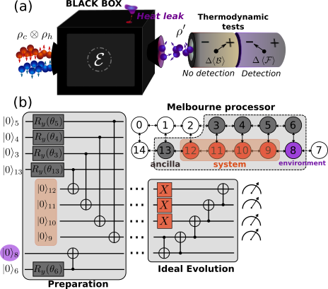
Figure 1: (a) Thermodynamic tests based on passive observables $\mathcal{F}$ operate as black box tests. This means that they provide unambiguous heat leak detection without knowing any detail on the dynamics, represented as a generic CPTP map $\mathcal{E}$. (b) The experiments implemented with the Melbourne processor involve ten qubits. For the preparation stage $R_{y}$ rotations by angles $\theta<\pi/2$ are applied to the qubits 3-6 and 13, which are then entangled with the system qubits (9-12) and the environment (qubit 8). After this circuit the system and the environment are left in states $\rho_{s}\sim\rho_{9}\otimes\rho_{10}\otimes\rho_{11}\otimes\rho_{12}$ and $\rho_{e}=\rho_{8}$, where $\rho_{8\leq i\leq 12}$ are thermal states at inverse temperatures $\beta_{i}$. The circuit for the evolution stage contains internal system gates and two cnots with the environment that generate the heat leak. In practice, this evolution results in a non-ideal transformation $\rho^{\prime}_{s}=\tilde{\mathcal{E}}_{s}(\rho_{s})$, that includes also internal errors.

Our experiments involve a preparation stage and an evolution stage. In the preparation stage the total system is initialized in the state $\rho_{se}=\rho_{s}\otimes\rho_{e}$, where $\rho_{s}=\otimes_{i}\frac{e^{-\beta_{i}H_{i}}}{Z_{i}}$, and $\rho_{e}=\frac{e^{-\beta_{e}H_{e}}}{Z_{e}}$ is a thermal state of the environment at inverse temperature $\beta_{e}$. In the evolution stage a global unitary $U_{se}$ is applied on $\rho_{se}$, which includes a system-environment interaction aimed to induce a heat leak. By measuring the final system state $\rho^{\prime}_{s}$ in the energy basis, the heat leak is observed if a violation $\textrm{Tr}[\mathcal{F}(\rho^{\prime}_{s}-\rho_{s})]<0$ occurs for at least one passive observable $\mathcal{F}$.

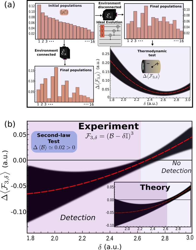
Figure 2: Heat leak tests performed in the Melbourne processor. (a) All the histograms depict measured system populations, averaged over the ten batches of preparation or evolution stages (each number $1\leq i\leq 16$ labels the same eigenstate in all histograms). The top left histogram shows the initial populations, sorted in decreasing order. The lower histogram shows the final populations when the environment coupling is switched on. If the environment is decoupled the final populations shown in the top right histogram are obtained. As expected, in this case no heat leak is observed using the test $\Delta\left\langle\mathcal{F}_{3,\delta}\right\rangle=\Delta\left\langle(\mathcal{B}-\delta\mathbb{I})^{3}\right\rangle$ (red dashed line), within a confidence interval of three standard deviations (shaded region). (b) When the environment is coupled, the same test yields detection in the interval $1.8\lesssim\delta\lesssim 2.6$ (same color coding of (a)). The inset shows the result for the simulation of the ideal evolution applied to $\{p_{i}^{s}\}$.

For the experiments performed with the Melbourne processor, the preparation and evolution stages are illustrated in Fig. 1(b). In this case we study a heat leak acting on a four-qubit system, due to the coupling with a single-qubit environment. The $i$th qubit in the system has Hamiltonian $H_{i}=|1\rangle_{i}\langle 1|$, where $|1\rangle_{i}$ is the excited state in the corresponding computational basis (setting the ground energy equal to zero). The total Hamiltonian of the system is simply $H_{s}=\sum_{i=9}^{12}H_{i}$. Accordingly, energy measurements are associated to measurements in the four-qubit computational basis $\{\otimes_{i=9}^{12}|j\rangle_{i}\}_{j=0,1}$. By default, all the qubits in the processor start in the ground state. This implies that direct preparation of mixed states is not possible. We circumvent this limitation by employing the qubits 3-6 and 13 as ancillae, to prepare the initial mixed state $\rho_{se}$. The procedure is indicated in Fig 1(b).

The IBMQE processors are subjected to gate errors and readout errors. In the case of the Melbourne processor, the employment of cnot gates for the preparation and the evolution introduces significant deviations from the ideal circuits. However, we certify that the initial state $\rho_{s}$ is well approximated by a product of thermal states with ground populations (with $p_{0}^{(i)}$ the ground population of qubit $i$) $p_{0}^{(12)}=0.612$, $p_{0}^{(11)}=0.586$, $p_{0}^{(10)}=0.611$, $p_{0}^{(9)}=0.557$, and that the environment is prepared in a thermal state $\rho_{e}$ with ground population $p_{0}^{e}=0.782$ (see Supplemental Material (sup, ) for further details). Since $\rho_{s}$ is compatible with Eq. (1), its deviation from the initial state programmed in the IBMQE software interface is irrelevant for the task of heat leak detection. To obtain the populations of $\rho_{s}$ and $\rho_{e}$, the readout error is modeled through a measurement matrix $\mathbb{M}$ that transforms the vector of actual (without readout error) populations $\{p_{i}^{s}\}=\{\langle i|_{s}\rho_{s}|i\rangle_{s}\}$ into observed (with readout error) populations $\mathbb{M}\{p_{i}^{s}\}$ (details about the experimental determination of this matrix are given in (sup, )). In this way, the actual populations are estimated by applying the inverse of $\mathbb{M}$ to the observed populations.

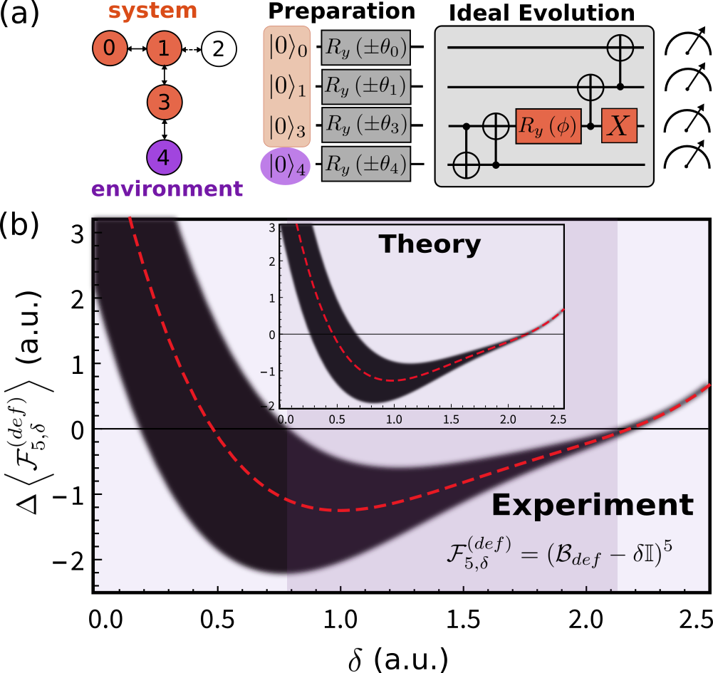
Figure 3: Heat leak tests performed in the five-qubit Essex processor. (a) We employ the qubits 0, 1, and 3 as system, and the qubit 4 as environment. The initial mixed state is prepared through single-qubit rotations $R_{y}(\pm\theta_{i})$, using the angles $\{\theta_{0},\theta_{1},\theta_{3},\theta_{4}\}=\{0.3\pi,0.4\pi,0.4\pi,0.15\pi\}$ (see text and (sup, )). (b) Heat leak test based on the observable $\mathcal{F}_{5,\delta}^{(def)}$, constructed from a passivity deformation $\mathcal{B}_{def}$ specified in the main text. This test detects the heat leak associated with the circuit in (a) within three standard deviations from $\Delta\left\langle\mathcal{F}_{5,\delta}^{(def)}\right\rangle$. The inset shows the result corresponding to the numerical simulation.

To construct the observable $\mathcal{B}=\sum_{i=1}^{16}-\textrm{ln}(p_{i}^{s})|i\rangle_{s}\langle i|$ and any passive observable ${\normalcolor{\color[rgb]{1,0,0}{\normalcolor\mathcal{F}_{\alpha,\delta}}}}$ we use the initial the populations $\{p_{i}^{s}\}$. As previously mentioned, due to the presence of gate errors the ideal evolution $U_{se}^{\textrm{id}}$ coded in the software interface is effectively implemented as a map ${\color[rgb]{1,0,0}{\normalcolor\tilde{\mathcal{E}}_{se}}}$ that yields the experimental final state ${\normalcolor{\color[rgb]{1,0,0}{\normalcolor\rho^{\prime}_{s}=\textrm{Tr}_{e}[\tilde{\mathcal{E}}_{se}(\rho_{se})]\equiv\tilde{\mathcal{E}}_{s}(\rho_{s})}}}$. The corresponding final distribution $\{p^{\prime}{}_{i}^{s}\}$ is also estimated by applying the inverse of the measurement matrix to the observed distribution. In this way, the test $\textrm{Tr}[{\color[rgb]{1,0,0}{\normalcolor\mathcal{F}_{\alpha,\delta}}}(\rho^{\prime}_{s}-\rho_{s})]$ is evaluated as

$$\Delta\left\langle\mathcal{F}_{\alpha,\delta}\right\rangle=\sum_{i=1}^{16}f_{\alpha,\delta}^{(i)}(p^{\prime}{}_{i}^{s}-p{}_{i}^{s}),$$ (4)

where $f_{\alpha,\delta}^{(i)}=(\mathcal{B}_{i}-\delta)^{\alpha}$ and $\mathcal{B}_{i}=-\textrm{ln}(p_{i}^{s})$. The experimental data are collected by implementing the circuits that include the preparation and evolution stages. We implement ten batches for each circuit, with each batch being composed of 8192 shots.

Figure 2 presents the experimental results of a heat leak test based on the observable $\mathcal{F}_{3,\delta}$. The histograms in Fig. 2(a) depict the initial populations $\{p_{i}^{s}\}$ and final populations $\{p^{\prime}{}_{i}^{s}\}$, given by normalized count frequencies from a total sample of $10\times 8192$ shots. The red dashed curves in Fig. 2 are obtained by plugging these populations into Eq. (4). Moreover, shaded regions in each plot stand for a confidence interval of three standard deviations (see (sup, )). In Fig. 2(a) it is shown that the test $\Delta\left\langle\mathcal{F}_{3,\delta}\right\rangle$ yields only positive values when the environment is decoupled, as expected. When the environment is coupled, Fig. 2(b) shows detection of the heat leak with the same test, for $1.8\lesssim\delta\lesssim 2.6$. Importantly, the application of this test is motivated by the fact that unambiguous detection (within the confidence interval) is not possible with the observable $\mathcal{F}_{2,\delta}$, based on the smaller power $\alpha=2$. The corresponding plot is provided in (sup, ). Moreover, for $\alpha=1$ the test $\Delta\left\langle\mathcal{F}_{1,\delta}\right\rangle=\Delta\left\langle\mathcal{B}\right\rangle$ also fails (see Fig. 2(b)). This clearly demonstrates a situation where global passivity outperforms the standard second law (2), regarding detection sensitivity. In (sup, ) it is also shown that for $0\leq\alpha\leq 4$ no detection occurs with the observables $\mathcal{B}^{\alpha}$.

Now we consider an experiment where passivity deformation outperforms both the second law and global passivity. Passivity deformation is a method to systematically construct passive observables, by performing suitable transformations on the eigenvalues of $\mathcal{B}$. In this work we employ the special deformation

$$\mathcal{B}\rightarrow\mathcal{B}_{def}=\sum_{i}\beta_{i}^{(def)}H_{i},$$ (5)

where $\beta_{i}^{(def)}$ are effective inverse temperatures that guarantee the passivity of $\mathcal{B}_{def}$. Figure 3(a) illustrates the structure of the Essex processor and the circuit used for the implementation of the heat leak, which involves a three-qubit system that interacts with a single-qubit environment. As explained below, detection with the test shown in Fig. 3(b) is possible thanks to the employment of a suitable deformation.

The limited size of the Essex processor prevents us to prepare the initial state $\rho_{s}\otimes\rho_{e}$ through entanglement with ancillae. However, a diagonal state of the form (1) can be obtained from an ensemble of coherent states with identical populations in the energy basis. We first separately prepare sixteen coherent states, by applying single-qubit rotations $\{R_{y}(\pm\theta_{i})\}_{i=0,1,3,4}$, see Fig. 3(a). As explained in (sup, ), by mixing these states with equal probabilities we obtain a product of thermal states with ground populations $p_{0}^{(i)}=\textrm{cos}^{2}(\theta_{i}/2)$. In this case four batches of 8192 shots are employed for each initial coherent state and its final counterpart.

In addition to the test shown in Fig. 3(b), we confirmed that the heat leak is not detected with the observable $\mathcal{B}$, neither with tests based on the observables $\mathcal{F}_{\alpha,\delta}=(\mathcal{B}-\delta\mathbb{I})^{\alpha}$, for $\alpha=2,3,4,5$. This difficulty is overcome through a deformation of $\mathcal{B}$, characterized by the transformation $\{\beta_{0},\beta_{1},\beta_{3}\}\rightarrow\{\beta_{0},0,\beta_{0}\}$. The resulting observable $\mathcal{B}_{def}=\beta_{0}(H_{1}+H_{3})$ is equivalent to the total Hamiltonian of the qubits 1 and 3. As occurs with the non-deformed observables $\mathcal{F}_{\alpha,\delta}$, the deformation $\mathcal{B}_{def}$ gives rise to a family of observables $\{\mathcal{F}_{\alpha,\delta}^{(def)}\}\equiv\{(\mathcal{B}_{def}-\delta\mathbb{I})^{\alpha}\}_{\alpha\geq 0}$ which are passive if the shift $\delta$ is properly chosen. These observables also exhibit a polynomial scaling similar to that described for $\mathcal{F}_{\alpha,\delta}$ (see (sup, )), with $n$ replaced by an effective number of qubits $n_{def}$ that satisfies $n_{def}\leq n$.

In Fig. 3(b) we use the same color coding as in Fig. 2(c). Clearly, for shift values $0.8\lesssim\delta\lesssim 2.1$ detection takes place with the deformed observable $\mathcal{F}_{5,\delta}^{(def)}$. In (sup, ) we also show that if the environment is decoupled the test $\Delta\left\langle\mathcal{F}_{5,\delta}^{(def)}\right\rangle$ is positive, as expected. This provides additional evidence that the source of the heat leak is the engineered environment interaction and not some intrinsic imperfection in the processor.

Finally, we remark that the advantage of shifted observables and deformed observables can be understood by explicitly writing the expansion

$$\Delta\left\langle(\mathcal{B}-\delta\mathbb{I})^{\alpha}\right\rangle=\sum_{k=0}^{\alpha}\left(\begin{array}[]{c}\alpha\\ k\end{array}\right)(-1)^{k}\delta^{k}\Delta\left\langle\mathcal{B}^{\alpha-k}\right\rangle,$$ (6)

which is valid for $\alpha$ positive and integer. Since for $k$ odd the factor $\left(\begin{array}[]{c}\alpha\\ k\end{array}\right)(-1)^{k}\delta^{k}$ is negative, the test $\Delta\left\langle(\mathcal{B}-\delta\mathbb{I})^{\alpha}\right\rangle$ can yield detection even if all the non-shifted tests $\Delta\left\langle\mathcal{B}^{\alpha-k}\right\rangle$ are positive. However, detection also requires that more weight is given to the negative factors than to the positive ones (associated with $\alpha$ even). The deformation $\mathcal{B}\rightarrow\mathcal{B}_{def}$ provides the appropriate weights $\Delta\left\langle\mathcal{B}_{def}^{\alpha-k}\right\rangle$ for this to happen, in the case of the second circuit analyzed.

Discussion. The TUR used in Ref. (Buffoni and Campisi, 2020) allows to conclude that for a certain annealing protocol the device operates as a thermal accelerator, if the annealer is prepared in a hot thermal state. Therefore, it can be asserted that the annealer does not evolve unitarily. This result relies on preliminary evidence that the background cold bath indeed affects the system dynamics. In particular, the application of the TUR requires to estimate first the temperature of this bath. Although we perform thermodynamic tests using an engineered enviroment, we stress that they provide unambiguous detection without any prior information on the potential source of noise.

Resource theory (RT) also provides an infinite set of thermodynamic constraints for systems coupled to a thermal bath through energy-preserving interactions (Brandao et al., 2015). In (sup, ) we show an example where no constraint from this infinite familiy can be violated by the presence of a hidden environment. Specifically, we study a four-qubit system that is divided into a “bath”, given by a subsystem at fixed temperature, and the remaining subsystem where the constraint is examined. The total system evolves through an energy-preserving circuit and an external interaction with a qubit environment. Importantly, even in cases where violations of RT constraints are observed they can be due to external classical drivings, and therefore such violations can also occur for unitary dynamics. For the studied example, we also show that the environment is detected using the passive observable $\mathcal{F}_{7,\delta}$.

Conclusions. In this work we experimentally show that thermodynamic inequalities recently derived (Uzdin and Rahav, 2018, 2019) are useful for the detection of heat leaks in quantum circuits. While the experiments are performed on small size circuits, we theoretically demonstrate efficient scalability to larger devices. In this context, error detection and characterization faces substantial experimental and computational challenges. These challenges are ultimately rooted in the exponential growth of resources needed to accurately estimate a quantum state or to simulate its evolution (Arute et al., 2019; Boixo et al., 2018; Zhong et al., 2020; Haah et al., 2017). However, several recent results show that certain quantum properties can be efficiently estimated, i.e. without incurring in an exponential overhead (Huang et al., 2020; Aaronson, 2019; Paini et al., 2020). The efficiency of the thermodynamic tests studied here builds up on such a possibility. Although they are specifically designed to detect non-unital dynamics, they are economic not only in terms of measurements, but also by saving the computational power required to compare experimental and simulated evolutions. A current limitation of these tests is that they cannot detect any non-unital error, see (sup, ). In addition, finding proper passive observables for detection in specfic situations is a non-trivial problem. These sensitity constraints can be interpreted as a “price to pay” in exchange for scalability, and further research concerning this trade-off is an interesting open problem. Apart from heat leaks, a pertinent question is if thermodynamic tools can be applied for diagnostics of other relevant errors, such as dephasing.

Supplemental Material

S-I Scaling of different heat leak tests with respect to system size

In the following we show that heat leak tests based on passive observables constitute an efficient method for the detection of non-unital errors in quantum devices. While in theory these errors can also be diagnosed using other more direct methods, we will also explain why such strategies are inefficient and become infeasible as the size of the system increases. More precisely,

• Direct methods such as quantum state tomography or quantum process tomography involve a number of measurements that grow exponentially with respect to the number of qubits $n$ in the system (Haah et al., 2017; O’Donnell and Wright, 2016). Such an exponential scaling is what we refer to as “inefficient”.

• Conversely, heat leak tests using passive observables are “efficient” in the sense that their measurement cost is polynomial with respect to $n$. Accordingly, these tests can be a more appealing and practical alternative for diagnostics of non-unital errors in large devices.

The basic tool to demonstrate the aforementioned efficiency is a theoretic-information result recently derived (Huang et al., 2020). This result refers to the number of measurements $N$ required to accurately estimate the mean values of a given set of $M$ observables $\{O_{i}\}_{1\leq i\leq M}$. Given a general quantum state state $\rho$,

$$N\sim\mathcal{O}\left(\frac{\textrm{log}(M/\mu)}{\epsilon^{2}}\textrm{max}_{i}\left\|O_{i}\right\|_{\textrm{shadow}}^{2}\right),$$ (S1)

measurements suffice to estimate all the mean values $\bigl{\langle}O_{i}\bigr{\rangle}=\textrm{Tr}[\rho O_{i}]$ with maximum error $\epsilon$. Specifically, in (Huang et al., 2020) it is shown that, if $N$ satisfies Eq. (S1), there is an explicit classical protocol that yields estimations $o_{i}$ of $\bigl{\langle}O_{i}\bigr{\rangle}$, such that $|o_{i}-\bigl{\langle}O_{i}\bigr{\rangle}|\leq\epsilon$ for $1\leq i\leq M$, with success probability $\textrm{Pr}\left(|o_{i}-\bigl{\langle}O_{i}\bigr{\rangle}|\leq\epsilon\right)\geq 1-\mu$. Equivalently, the protocol achieves $|o_{i}-\bigl{\langle}O_{i}\bigr{\rangle}|\leq\epsilon$ with maximum failure probability $\mu$.

The observables $O_{i}$ can be arbitrary and the “shadow norm” $\left\|\cdot\right\|_{\textrm{shadow}}$ is determined by the specific measurement procedure. For passive observables derived from GP and PD, we show in Section B of this appendix that the corresponding estimation can be obtained from the simultaneous estimation of $M=n\frac{n^{\alpha}-1}{n-1}$ local observables $O_{i}$, where $\alpha$ is the maximum number of qubits on which these observables act non-trivially. In this case, a suitable measurement procedure (explained in Section B) yields a norm $\left\|O_{i}\right\|_{\textrm{shadow}}^{2}$ whose maximum depends only on $\alpha$. Thus, we can combine Eq. (S1) with error propagation, to show in Section B that estimating the mean value of passive observables involves the polynomial measurement cost given in Eq. (S11). This implies that the corresponding heat leak tests can also be efficiently evaluated.

S-I.1 Direct methods for the detection of heat leaks (non-unital errors) and experimental cost

Detection via quantum state tomography. As explained in the main text, heat leaks are associated with transformations $\rho\rightarrow\rho^{\prime}$ that cannot be written as $\rho^{\prime}=\sum_{k}\text{$\lambda$}_{k}U_{k}\rho U_{k}^{\dagger}$, where $\{\lambda_{k}\}$ are probabilities and $\{U_{k}\}$ are unitary maps. The criterion of majorization provides a theoretical tool to directly check if $\rho\rightarrow\rho^{\prime}$ contains a heat leak. Specifically, let $\{r_{i}^{\downarrow}\}$ and $\{r^{\prime}{}_{i}^{\downarrow}\}$ denote respectively the eigenvalues of $\rho$ and $\rho^{\prime}$, arranged in non-increasing order: $r_{i}^{\downarrow}\geq r_{i+1}^{\downarrow}$ and $r_{i}^{\prime}{}^{\downarrow}\geq r^{\prime}_{i+1}{}^{\downarrow}$ for all $1\leq i\leq d$. The state $\rho$ majorizes the state $\rho^{\prime}$, denoted as $\rho\succ\rho^{\prime}$, iff $S_{j}\equiv\sum_{i=1}^{j}r_{i}^{\downarrow}\geq S^{\prime}_{j}\equiv\sum_{i=1}^{j}r^{\prime}{}_{i}^{\downarrow}$ for all $1\leq j\leq d$ (Nielsen, 2002; Marshall et al., 1979). Since $\rho\succ\rho^{\prime}$ iff there exist $\{\lambda_{k}\}$ and $\{U_{k}\}$ such that $\rho^{\prime}=\sum_{k}\text{$\lambda$}_{k}U_{k}\rho U_{k}^{\dagger}$ (Nielsen, 2002), any heat leak manifests itself in an inequality $S_{j}<S^{\prime}_{j}$, for some $1\leq j\leq d$. However, knowing the partial sums $\{S^{\prime}_{j}\}_{1\leq j\leq d}$ requires to know both the initial and final eigenvalues $\{r_{i}{}^{\downarrow}\}$ and $\{r_{i}^{\prime}{}^{\downarrow}\}$.

The experimental determination of $\{r^{\prime}_{i}{}^{\downarrow}\}$ involves in the worst case quantum state tomography (state tomography for simplicity) of the final state $\rho^{\prime}$, which consists in a full experimental reconstruction of $\rho^{\prime}$. Of course this is also true for the eigenvalues of the initial state $\rho$. From fundamental information-theoretic bounds it is known that at least $N\sim\mathcal{O}(\textrm{rank}(\rho^{\prime})d)$ measurements are required for state tomography (Haah et al., 2017). For example, if $\rho^{\prime}$ describes a system of $n$ qubits, the number of measurements needed grows exponentially with $n$. In particular, this makes state tomography infeasible for detecting heat leaks in quantum devices sufficiently large to perform useful tasks.

Detection via population estimation in the computational basis. Some heat leaks could in principle be diagnosed by checking a violation of majorization between the initial state and the diagonal part of $\rho^{\prime}$ in a suitable basis. In a quantum processor, the natural choice to measure the diagonal of $\rho^{\prime}$ is the computational basis, where measurements can be directly performed (measurements in other bases involve pre-measurement gates that can introduce additional errors). Let $\{|i_{\textrm{c}}\rangle\}_{1\leq i\leq d}$ denote the computational basis, and $s_{i}=\langle i_{\textrm{c}}|\rho^{\prime}|i_{\textrm{c}}\rangle$ the $i$th diagonal element of $\rho^{\prime}$ in this basis. Moreover, let $D(\rho^{\prime})$ be the diagonal matrix whose entries are given by the $s_{i}$. Since $D(\rho^{\prime})$ is simply $\rho^{\prime}$ dephased in the computational basis, it can be written as a mixture of unitaries acting on $\rho^{\prime}$ (Watrous, 2018), which also implies that $\rho^{\prime}\succ D(\rho^{\prime})$. From transitivity of majorization, it follows that if $\rho\succ\rho^{\prime}$ then $\rho\succ D(\rho^{\prime})$.

Using the populations $s_{i}$ one can detect a heat leak if a relation of the form $\sum_{i=1}^{j}r_{i}^{\downarrow}<\sum_{i=1}^{j}s_{i}^{\downarrow}$ holds, for some $1\leq j\leq d$. While this technique is clearly more economic than state tomography of $\rho^{\prime}$, for a system of $n$ qubits a reconstruction of all the partial sums $\sum_{i=1}^{j}s_{i}^{\downarrow}$ still involves measuring $2^{n}-1$ populations $s_{i}$ (with one of them deduced by normalization). In the following appendix we will discuss in more detail the experimental cost of this method, since there is a connection between the inequalities $\sum_{i=1}^{j}r_{i}^{\downarrow}<\sum_{i=1}^{j}s_{i}^{\downarrow}$ and the heat leaks that can be detected using passive observables. In particular, we will show that even for a single value of $j$ it is necessary to estimate all the final populations $s_{i}$, to unambiguosly evaluate the partial sum $\sum_{i=1}^{j}s_{i}^{\downarrow}$.

Quantum process tomography and transfer matrix. Perhaps the most direct route for error characterization in any quantum device would be to perform quantum process tomography, or process tomography for brevity. This consists in the full experimental characterization of a quantum process. If this process is represented by a quantum channel $\mathcal{E}$ that maps density matrices into density matrices, process tomography aims at determining the action of $\mathcal{E}$ on any possible initial state $\rho$. To that end the channel must be implemented on $d^{2}$ states that form a tomographically complete basis (Nielsen and Chuang, 2010), and state tomography must be applied on each of the corresponding $d^{2}$ outputs. From the previous discussion on state tomography it is clear that the scaling of process tomography is even worse. The discussion regarding the inefficiency of population measurements leads to an analogous conclusion for the transfer matrix, which may be seen a coarse-grained version of $\mathcal{E}$. The transfer $T$ matrix is $d\times d$ matrix with elements $T_{ij}\equiv\textrm{Tr}\left[|i_{\textrm{c}}\rangle\langle i_{\textrm{c}}|\mathcal{E}(|j_{\textrm{c}}\rangle\langle j_{\textrm{c}}|)\right]$. To reconstruct $T$, the process $\mathcal{E}$ must be implemented on the $d=2^{n}$ computational eigenstates and the final populations $T_{ij}$ have to be measured. This implies that measuring $T$ is not a practical alternative for error detection even for systems of moderate size.

S-I.2 Efficient evaluation of heat leak tests based on passive observables

To understand why passive observables $\mathcal{F}=\mathcal{F}_{\alpha,\delta}$ and $\mathcal{F}=\mathcal{F}_{\alpha,\delta}^{(def)}$ are an efficient tool for heat leak detection we must first describe the relevant parameters entering the operator norm $\left\|\cdot\right\|_{\textrm{shadow}}$ in Eq. (S1). As a matter of fact, we will see that for passive observables this norm is upper bounded by a constant that is independent of $d$. In what follows we refer to the final state $\rho^{\prime}$, which yields the final mean value $\bigl{\langle}\mathcal{F}\bigr{\rangle}^{\prime}=\textrm{Tr}(\mathcal{F}\rho^{\prime})$. However, the same arguments are valid for the initial mean value $\bigl{\langle}\mathcal{F}\bigr{\rangle}=\textrm{Tr}(\mathcal{F}\rho)$.

The experimental procedure underlying Eq. (S1) is based on measuring $\rho^{\prime}$ in $N$ randomly chosen measurement bases (Huang et al., 2020). These bases are determined by randomly selecting unitaries $U$ from some ensemble $\mathcal{U},$and then measuring the transformed state $U\rho^{\prime}U^{\dagger}$ in the computational basis (this effectively implements a measurement in the rotated basis $\{U^{\dagger}|i_{\textrm{c}}\rangle\}$). Afterwards, a classical postprocessing is applied to the $N$ outcomes to obtain estimated mean values $\{o_{i}\}_{1\leq i\leq M}$ with maximum error $\epsilon$ and maximum failure probability $\mu$.

Lemma 1 (based on the results from (Huang et al., 2020)). The norm $\left\|\cdot\right\|_{\textrm{shadow}}$ depends on the ensemble of unitaries $\mathcal{U}$. In Ref. (Huang et al., 2020) the authors consider two ensembles: arbitrary Clifford unitaries acting on $n$ qubits, and tensor products of single-qubit Clifford unitaries. In the second case the ($n$-qubit) measurement bases are random tensor products of Pauli bases $\{X,Y,Z\}$. For this choice, the norm $\left\|\cdot\right\|_{\textrm{shadow}}$ depends only on the locality of the observable $O$ and not on the dimension $d$. Specifically, for an observable $O=\tilde{O}\otimes\mathbb{I}^{n-k}$, where $\tilde{O}$ acts non trivially on $k$ qubits and $\mathbb{I}^{n-k}$ is the identity on the remaining $n-k$ qubits, $\left\|O\right\|_{\textrm{shadow}}^{2}\leq 4^{k}\left\|O\right\|_{\infty}^{2}$, being $\left\|\cdot\right\|_{\infty}$ the spectral norm (Proposition 3 in (Huang et al., 2020)).

A passive observable $\mathcal{F}_{\alpha,\delta}$ is a sum of local observables acting on $k\leq\alpha$ qubits. This is deduced by explicitly writing the binomial expansion for $\mathcal{F}_{\alpha,\delta}=(\mathcal{B}-\delta\mathbb{I})^{\alpha}$:

$$\mathcal{F}_{\alpha,\delta} =(\mathcal{B}-\delta\mathbb{I})^{\alpha}$$

$$=\sum_{k=0}^{\alpha}\left(\begin{array}[]{c}\alpha\\ k\end{array}\right)(-1)^{\alpha-k}\delta^{\alpha-k}\mathcal{B}^{k}.$$ (S4)

From the definition of $\mathcal{B}$, $\mathcal{B}=\sum_{i=1}^{n}\beta_{i}H_{i}$, we also have that

$$\mathcal{B}^{k} =\left(\sum_{i=1}^{n}\beta_{i}H_{i}\right)^{k}$$

$$=\sum_{i_{1}=1}^{n}\sum_{i_{2}=1}^{n}...\sum_{i_{k}=1}^{n}\left(\otimes_{m=1}^{k}\beta_{i_{m}}H_{i_{m}}\right)$$

$$=\sum_{\{i_{m}\}}\left(\prod_{m=1}^{k}\beta_{i_{m}}\right)\tilde{\mathcal{H}}_{k,\{i_{m}\}},$$

where $\tilde{\mathcal{H}}_{k,\{i_{m}\}}\equiv\otimes_{m=1}^{k}H_{i_{m}}$and the sum $\sum_{\{i_{m}\}}$ is over the $n^{k}$ sets of indices $\{i_{m}\}_{1\leq m\leq k}$ that label groups of $k$ qubits. Therefore, $\mathcal{B}^{k}$ is a sum of $n^{k}$ observables that act locally on sets of $k$ qubits.

An estimation of the mean value $\bigl{\langle}\mathcal{F}_{\alpha,\delta}\bigr{\rangle}$ can be constructed from the estimation of all the mean values $\bigl{\langle}\tilde{\mathcal{H}}_{k,\{i_{m}\}}\bigr{\rangle}$. This has to be done carefully, keeping in mind that the errors for the $\bigl{\langle}\tilde{\mathcal{H}}_{k,\{i_{m}\}}\bigr{\rangle}$ propagate to $\bigl{\langle}\mathcal{F}_{\alpha,\delta}\bigr{\rangle}$. However, we show that if $N$ measurements allow to estimate $\left\{\bigl{\langle}\tilde{\mathcal{H}}_{k,\{i_{m}\}}\bigr{\rangle}\right\}$ with accuracy $(\epsilon,\mu)$, the same accuracy can be achieved on $\bigl{\langle}\mathcal{F}_{\alpha,\delta}\bigr{\rangle}$ if $N$ is increased to $N^{\prime}$, with an increment that is only polynomial in $n$. Accordingly, efficient estimation of $\left\{\bigl{\langle}\tilde{\mathcal{H}}_{k,\{i_{m}\}}\bigr{\rangle}\right\}$ implies efficient estimation of $\bigl{\langle}\mathcal{F}_{\alpha,\delta}\bigr{\rangle}$. We show first that

$$N\sim\mathcal{O}\left(\frac{\textrm{log}(n/\mu)}{\epsilon^{2}}\right).$$ (S5)

To this end we use the fact that the norm $\left\|\tilde{\mathcal{H}}_{k,\{i_{m}\}}\right\|_{\textrm{shadow}}^{2}$ satisfies $\left\|\tilde{\mathcal{H}}_{k,\{i_{m}\}}\right\|_{\textrm{shadow}}^{2}\leq 4^{k}$, which follows from Lemma 1 and the fact that $\left\|\otimes_{m=1}^{k}H_{i_{m}}\right\|_{\infty}=1$ (since by convention the maximum eigenvalue of each $H_{i_{m}}$ is 1). Hence, $\textrm{max}_{1\leq k\leq\alpha,\{i_{m}\}}\left\|\tilde{\mathcal{H}}_{k,\{i_{m}\}}\right\|_{\textrm{shadow}}^{2}$ is independent of $n$ and can be absorbed in the implicit constants of Eq. (S1). On the other hand, there are $n^{k}$ observables$\tilde{\mathcal{H}}_{k,\{i_{m}\}}$ for $k$ fixed, which yields the total number

$$M=\sum_{k=1}^{\alpha}n^{k}=n^{\alpha}\sum_{k=0}^{\alpha-1}\left(\frac{1}{n}\right)^{k}=n\frac{n^{\alpha}-1}{n-1}.$$

For $n$ large, it is straightforward to check that $\textrm{log}(M)\sim\alpha\textrm{log}(n)$. By inserting this into Eq. (S1) we obtain Eq. (S5).

Now we proceed to determine the (order of the) number of measurements $N^{\prime}$ to estimate $\bigl{\langle}\mathcal{F}_{\alpha,\delta}\bigr{\rangle}$ keeping accuracy $(\epsilon,\mu)$. Let $\tilde{H}_{k,\{i_{m}\}}$ and $F_{\alpha,\delta}$ denote respectively the estimations of the mean values $\bigl{\langle}\tilde{\mathcal{H}}_{k,\{i_{m}\}}\bigr{\rangle}$ and $\bigl{\langle}\mathcal{F}_{\alpha,\delta}\bigr{\rangle}$. If we require that $\bigl{|}\tilde{H}_{k,\{i_{m}\}}-\bigl{\langle}\tilde{\mathcal{H}}_{k,\{i_{m}\}}\bigr{\rangle}\bigr{|}\leq\epsilon$ with probability $\textrm{Pr}\left(\bigl{|}\tilde{H}_{k,\{i_{m}\}}-\bigl{\langle}\tilde{\mathcal{H}}_{k,\{i_{m}\}}\bigr{\rangle}\bigr{|}\leq\epsilon\right)\geq 1-\mu$ for all $k,\{i_{m}\}$, then $\bigl{|}F_{\alpha,\delta}-\bigl{\langle}\mathcal{F}_{\alpha,\delta}\bigr{\rangle}\bigr{|}\leq\epsilon_{\textrm{tot}}$ with probability $\textrm{Pr}\left(|F_{\alpha,\delta}-\bigl{\langle}\mathcal{F}_{\alpha,\delta}\bigr{\rangle}|\leq\epsilon_{\textrm{tot}}\right)\geq 1-\mu$. The total error $\epsilon_{\textrm{tot}}$ is additive because $\mathcal{F}_{\alpha,\delta}$ is a linear combination of $\tilde{\mathcal{H}}_{k,\{i_{m}\}}$ and this linearity extends to the mean value. That is,

$$\bigl{\langle}\mathcal{F}_{\alpha,\delta}\bigr{\rangle}=\sum_{k=0}^{\alpha}\sum_{\{i_{m}\}}c_{k,\{i_{m}\}}^{(\alpha,\delta)}\bigl{\langle}\tilde{\mathcal{H}}_{k,\{i_{m}\}}\bigr{\rangle},$$ (S6)

where $c_{k,\{i_{m}\}}^{(\alpha,\delta)}\equiv\left(\begin{array}[]{c}\alpha\\ k\end{array}\right)(-\delta)^{\alpha-k}\prod_{m=1}^{k}\beta_{i_{m}}$. Next, we multiply each inequality $\bigl{|}\tilde{H}_{k,\{i_{m}\}}-\bigl{\langle}\tilde{\mathcal{H}}_{k,\{i_{m}\}}\bigr{\rangle}\bigr{|}\leq\epsilon$ by the coefficient $c_{k,\{i_{m}\}}^{(\alpha,\delta)}$ and take the sum over $k$ and $\{i_{m}\}$, which leads to the expression $\bigl{|}F_{\alpha,\delta}-\bigl{\langle}\mathcal{F}_{\alpha,\delta}\bigr{\rangle}\bigr{|}\leq\sum_{k,\{i_{m}\}}\bigl{|}c_{k,\{i_{m}\}}^{(\alpha,\delta)}\bigr{|}\epsilon$. The quantity $\sum_{k,\{i_{m}\}}\bigl{|}c_{k,\{i_{m}\}}^{(\alpha,\delta)}\bigr{|}\epsilon$ thus determines the maximum total error $\epsilon_{\textrm{tot}}$. By applying the bound $c_{k,\{i_{m}\}}^{(\alpha,\delta)}\leq\textrm{max}_{k,\{i_{m}\}}\left(\prod_{m=1}^{k}\beta_{i_{m}}\right)\left(\begin{array}[]{c}\alpha\\ k\end{array}\right)(-\delta)^{\alpha-k}$, we conclude that

$$\frac{\epsilon_{\textrm{tot}}}{\epsilon} \leq\textrm{max}_{\{i_{m}\}}\left(\prod_{m=1}^{k}\beta_{i_{m}}\right)\sum_{k=0}^{\alpha}\left(\begin{array}[]{c}\alpha\\ k\end{array}\right)(\delta)^{\alpha-k}n^{k}$$ (S9)

$$=\textrm{max}_{\{i_{m}\}}\left(\prod_{m=1}^{k}\beta_{i_{m}}\right)(n+\delta)^{\alpha}.$$ (S10)

Equation (S10) indicates that if each estimated value $\tilde{H}_{k,\{i_{m}\}}$ has maximum error $\epsilon$, the maximum error corresponding to $F_{\alpha,\delta}$ has an upper bound that grows polynomially in $n$. On the other hand, the minimum success probability is reduced to $1-\mu_{\textrm{tot}}=(1-\mu)^{n\frac{n^{\alpha}-1}{n-1}}$. This decrement in accuracy for $F_{\alpha,\delta}$ can be compensated by imposing a higher accuracy $(\epsilon^{\prime},\mu^{\prime})$ for the estimation of each $\bigl{\langle}\tilde{\mathcal{H}}_{k,\{i_{m}\}}\bigr{\rangle}$, such that $(\epsilon_{\textrm{tot}},\mu_{\textrm{tot}})=(\epsilon,\mu)$. If we perform the substitutions $\epsilon_{\textrm{tot}}\rightarrow\epsilon$ and $\epsilon\rightarrow\epsilon^{\prime}$, Eq. (S10) yields the lower bound $\epsilon^{\prime}\geq\frac{\epsilon}{\textrm{max}_{\{i_{m}\}}\left(\prod_{m=1}^{k}\beta_{i_{m}}\right)(n+\delta)^{\alpha}}$. Moreover, from $1-\mu=(1-\mu^{\prime})^{n\frac{n^{\alpha}-1}{n-1}}$ we obtain $\mu^{\prime}=1-(1-\mu)^{\frac{n-1}{n(n^{\alpha}-1)}}$. The Taylor expansion of this expression around zero yields $\mu^{\prime}\sim\frac{n-1}{n(n^{\alpha}-1)}\mu$, for $\mu\ll 1$. In this way, the number of measurements required to estimate $\bigl{\langle}\mathcal{F}_{\alpha,\delta}\bigr{\rangle}$ with accuracy $(\epsilon,\mu)$ is

$$N^{\prime}\sim\mathcal{O}\left(\frac{\textrm{log}(n/\mu^{\prime})}{\epsilon^{\prime 2}}\right)=\mathcal{O}\left(\frac{\textrm{log}(n/\mu)}{\epsilon{}^{2}}(n+\delta)^{2\alpha}\right),$$ (S11)

where we have made the approximation $\textrm{log}\left(\frac{n(n^{\alpha}-1)}{n-1}\right)\sim\alpha\textrm{log}(n)$. Note also that the quantity $\textrm{max}_{\{i_{m}\}}\left(\prod_{m=1}^{k}\beta_{i_{m}}\right)$ can be absorbed with the other implicit constants that do not depend on $n$.

Equation (S11) is the main result of this appendix. It tells us that we can accurately estimate $\bigl{\langle}\mathcal{F}_{\alpha,\delta}\bigr{\rangle}$ with a number of measurements that scales polynomially in the number of qubits, irrespective of the state on which $\bigl{\langle}\mathcal{F}_{\alpha,\delta}\bigr{\rangle}$ is evaluated. In addition to $F_{\alpha,\delta}$, let $F^{\prime}_{\alpha,\delta}$ denote the estimation of the final mean values $\bigl{\langle}\mathcal{F}_{\alpha,\delta}\bigr{\rangle}^{\prime}=\textrm{Tr}(\rho^{\prime}\mathcal{F}_{\alpha,\delta})$. If we require that $F^{\prime}_{\alpha,\delta}$ also has accuracy $(\epsilon,\mu)$, the estimation of the test $\Delta\bigl{\langle}\mathcal{F}_{\alpha,\delta}\bigr{\rangle}=\bigl{\langle}\mathcal{F}_{\alpha,\delta}\bigr{\rangle}^{\prime}-\bigl{\langle}\mathcal{F}_{\alpha,\delta}\bigr{\rangle}$, denoted as $\Delta F_{\alpha,\delta}$, has accuracy $(2\epsilon,(1-\mu)^{2})$. Therefore, this test can also be accurately evaluated with $N^{\prime}$ given by Eq. (S11).

Summarizing, the estimation of $\Delta\bigl{\langle}\mathcal{F}_{\alpha,\delta}\bigr{\rangle}$ involves two stages. A first one that could be referred to as “direct estimation”, which is applied to the observables $\{\tilde{\mathcal{H}}_{k,\{i_{m}\}}\}_{1\leq k\leq\alpha,\{i_{m}\}}$, with $\tilde{\mathcal{H}}_{k,\{i_{m}\}}=\otimes_{m=1}^{k}H_{i_{m}}$ an arbitrary product of $k$ single-qubit Hamiltonians. Equation (S5) provides the order of the number of measurements required to simultaneously produce all the (initial and final) estimated values $\{\tilde{H}_{k,\{i_{m}\}}\}$, with accuracy $(\epsilon,\mu)$. The second “indirect estimation” stage consists of using Eq. (S6) to obtain $\Delta F_{\alpha,\delta}$ from $\{\tilde{H}_{k,\{i_{m}\}}\}$. Due to error propagation, to achieve accuracy $(2\epsilon,(1-\mu)^{2})$ in the estimation of $\Delta\bigl{\langle}\mathcal{F}_{\alpha,\delta}\bigr{\rangle}$ each $\tilde{H}_{k,\{i_{m}\}}$ must be characterized by higher accuracy $(\epsilon^{\prime},\mu)$, such that the number of measurements needed increases to the value given in Eq. (S11). For a fixed $\alpha$ there are indeed infinite passive observables whose corresponding tests can be simultaneously evaluated. This is a consequence of the two observations stated below. Importantly, we must keep in mind that $\alpha$ is a positive integer and $\delta$ is a positive real number.

• For $\alpha=\alpha_{\textrm{max}}$, direct estimation yields the set $\{\tilde{H}_{k,\{i_{m}\}}\}_{1\leq k\leq\alpha_{\textrm{max}},\{i_{m}\}}$, which includes all the estimated values $\{\tilde{H}_{k,\{i_{m}\}}\}_{1\leq k\leq\alpha,\{i_{m}\}}$, $\alpha\leq\alpha_{\textrm{max}}$. This allows to obtain all the $\{\Delta F_{\alpha,\delta}\}_{\alpha\leq\alpha_{\textrm{max}}}$ for a certain value of $\delta$, using Eq. (S6).

• Let us rewrite $N^{\prime}$ in Eq. (S11) as $N^{\prime}(\alpha,\delta)$, to make explicit the dependence on $\alpha$ and $\delta$. Since $N^{\prime}(\alpha,\delta)\leq N^{\prime}(\alpha_{\textrm{max}},\delta_{\textrm{max}})$ for $\alpha\leq\alpha_{\textrm{max}}$ and $\delta\leq\delta_{\textrm{max}}$, $N^{\prime}(\alpha_{\textrm{max}},\delta_{\textrm{max}})$ measurements suffice to obtain any estimated value $\{\Delta F_{\alpha,\delta}\}_{\alpha\leq\alpha_{\textrm{max}},\delta\leq\delta_{\textrm{max}}}$, with accuracy $(2\epsilon,(1-\mu)^{2})$, by applying Eq. (S6).

We also remark that the previous procedure is directly applicable to the deformed observables $\mathcal{F}_{\alpha,\delta}^{(def)}$. In this case the only difference is that Eq. (S6) must be applied using coefficients $c_{k,\{i_{m}\}}^{(\alpha,\delta)}=\left(\begin{array}[]{c}\alpha\\ k\end{array}\right)(-\delta)^{\alpha-k}\prod_{m=1}^{k}\beta_{i_{m}}^{(def)}$, where $\{\beta_{i}^{(def)}\}$ are the effective temperatures that characterize a given deformation. Importantly, if there are sufficiently hot qubits in the initial state it is possible to use deformations that set the corresponding temperatures to zero (Uzdin and Rahav, 2018), i.e. $\beta_{i}\rightarrow\beta_{i}^{(def)}=0$. This is illustrated in the second experiment of the main text with the inverse temperature $\beta_{1}$. For such deformations, $\mathcal{B}$ is transformed into $\mathcal{B}_{def}=\sum^{\prime}_{i}\beta_{i}^{(def)}H_{i}$, where prime in the sum indicates that it convers only a subset of qubits. If $n_{def}$ denotes the number of qubits in this subset, the substitution of $\mathcal{B}$ by $\mathcal{B}_{def}$ in Eq. (S4) leads to analogous of Eqs. (S10) and (S11) where $n$ is replaced by $n_{def}$. Accordingly, some deformations can significantly reduce the measurement cost $N^{\prime}$ if $n_{def}\ll n$.

S-II sensitivity of heat leak tests using passive observables and practical advantage

In this appendix we characterize an infinite family of heat leaks whose diagnostics is inefficient using population estimation, i.e. it requires a number of measurements of order $\mathcal{O}(2^{n})$. Moreover, by construction such heat leaks are detectable using passive observables. This illustrates a situation where the efficiency of the method can be fully exploited for actual detection.

We start by analyzing the complexity of the method described in the previous appendix, which provides detection if the inequality $\sum_{i=1}^{j}r_{i}^{\downarrow}<\sum_{i=1}^{j}s_{i}^{\downarrow}$ holds for some $1\leq j\leq 2^{n}$. Since $\rho$ is diagonal in the computational basis (cf. Eq. (1) of the main text), the most convenient choice is $s_{i}^{\downarrow}=p^{\prime}{}_{i}^{\downarrow}$, where $p^{\prime}_{i}=\textrm{Tr}(|i_{\textrm{c}}\rangle\langle i_{\textrm{c}}|\rho)$ (for simplicity we also write $r_{i}^{\downarrow}=p_{i}^{\downarrow}$, with $p_{i}=\textrm{Tr}(|i_{\textrm{c}}\rangle\langle i_{\textrm{c}}|\rho)$). Accordingly, the following recipe could be applied to heat leak diagnostics:

1. Estimate the initial and final populations $\{p_{i}\}$ and $\{p^{\prime}_{i}\}$.

2. Sort them in non-increasing order.

3. Evaluate the quantities $\xi_{j}\equiv\sum_{i=1}^{j}p{}_{i}^{\prime\downarrow}-\sum_{i=1}^{j}p{}_{i}^{\downarrow}$. If $\xi_{j}>0$ for some $1\leq j\leq 2^{n}$, there is a heat leak. If $\xi_{j}\leq 0$ for $1\leq j\leq 2^{n}$, there can be a heat leak that is undetectable using this method. This kind of heat leak corresponds to a transformation such that $\rho^{\prime}$ is not majorized by $\rho$, yet the majorization relation $\rho\succ D(\rho^{\prime})$ (which is equivalent to $\xi_{j}\leq 0$ for $1\leq j\leq 2^{n}$ ) holds.

Step 1 requires to estimate the $M=2^{n}-1$ mean values $\bigl{\langle}|i_{\textrm{c}}\rangle\langle i_{\textrm{c}}|\bigr{\rangle}$ for the initial and final states. This number contributes to $N$ in Eq. (S1) with a term that is linear in $n$. However, the shadow norm for projectors $|i_{\textrm{c}}\rangle\langle i_{\textrm{c}}|$ is exponential in $n$, for both Pauli measurements and measurements based on general Clifford unitaries (Huang et al., 2020). This implies that population estimation is inefficient with the method developed in (Huang et al., 2020). On the other hand, it has recently been pointed out that a single population can be efficiently estimated employing a different technique (Paini et al., 2020). The key obstacle is that the results presented in (Paini et al., 2020) apply to single observables, and step 1 refers to exponentially many observables. Crucially, even for a single value of $j$ the quantity $\xi_{j}$ can be unambiguosly evaluated only if all the populations have been estimated. For example, suppose that one chooses randomly a set of projectors $\{|i_{\textrm{c}}\rangle\langle i_{\textrm{c}}|\}_{i\in I}$, where $I=\{i_{1},i_{2},...,i_{j}\}\subset\{1,2,...,2^{n}-1\}$ is some arbitrary set of $j\ll 2^{n}$ indices. From the corresponding populations one can be certain that the sum $\sum_{i\in I}p^{\prime}_{i}$ equals $\sum_{i=1}^{j}p{}_{i}^{\prime\downarrow}$, without measuring any other population, iff

$$1-\sum_{i\in I}p^{\prime}_{i}\leq\textrm{min}_{i\in I}p^{\prime}_{i}.$$

When this inequality is satisfied, it can be combined with the relation $\textrm{max}_{i\notin I}p^{\prime}_{i}\leq\sum_{i\notin I}p^{\prime}_{i}=1-\sum_{i\in I}p^{\prime}_{i}$ to conclude that $\textrm{max}_{i\notin I}p^{\prime}_{i}\leq\textrm{min}_{i\in I}p^{\prime}_{i}$. Therefore, $\sum_{i\in I}p^{\prime}_{i}$ contains indeed the largest $j$ populations. Conversely, if $1-\sum_{i\in I}p^{\prime}_{i}>\textrm{min}_{i\in I}p^{\prime}_{i}$, it is possible that $\textrm{max}_{i\notin I}p^{\prime}_{i}>\textrm{min}_{i\in I}p^{\prime}_{i}$, and $\sum_{i\in I}p^{\prime}_{i}\neq\sum_{i=1}^{j}p{}_{i}^{\prime\downarrow}$. However, without prior information about $\rho^{\prime}$ it is extremely unlikely that the set $I$ corresponds to $\{p{}_{i}^{\prime\downarrow}\}_{1\leq i\leq j}$, since this is just one among $\frac{\left(2^{n}-1\right)!}{\left(2^{n}-1-j\right)!j!}$ possible sets of $j$ projectors. This allows us to conclude that the evaluation of $\xi_{j}$ is inefficient.

Sensitivity of heat leak tests using passive observables. Let us now characterize the class of heat leaks that can be diagnosed by performing tests $\Delta\bigl{\langle}\mathcal{F}\bigr{\rangle}$. Although we previously showed that this can be done efficiently, it is important to understand the fundamental limits on sensitivity for these tests. If $f_{i}$ denotes the eigenvalue of $\mathcal{F}$ corresponding to the eigenstate $|i_{\textrm{c}}\rangle$, by definition

$$\Delta\bigl{\langle}\mathcal{F}\bigr{\rangle}=\sum_{i=1}^{d}f_{i}\Delta p_{i},$$ (S12)

where $\Delta p_{i}=\textrm{Tr}[|i_{\textrm{c}}\rangle\langle i_{\textrm{c}}|(\rho^{\prime}-\rho)]$. For our purpose it is covenient to write $\Delta\bigl{\langle}\mathcal{F}\bigr{\rangle}$ in a different manner. By defining $\Delta f_{k}\equiv f_{k+1}-f_{k}$, we have that $f_{i}=f_{0}+\sum_{k=0}^{i-1}\Delta f_{k}$, where $f_{0}$ is just a reference value that won’t appear in the final expression. The substitution of $f_{i}$ by $f_{0}+\sum_{k=0}^{i-1}\Delta f_{k}$ in Eq. (S12) yields

$$\Delta\bigl{\langle}\mathcal{F}\bigr{\rangle} =\sum_{i=1}^{d}\left(\sum_{j=0}^{i-1}\Delta f_{j}\right)\Delta p_{i}+f_{0}\sum_{i=1}^{d}\Delta p_{i}$$

$$=\sum_{j=1}^{d-1}\Delta f_{j}\left(\sum_{i=j+1}^{d}\Delta p_{i}\right)$$

$$=-\sum_{j=1}^{d-1}\Delta f_{j}\bar{\xi}_{j},$$

where $\bar{\xi}_{j}\equiv\Delta\sum_{i=1}^{j}p_{i}$.

It is interesting to compare the quantity $\bar{\xi}_{j}$ with $\xi_{j}$, previously introduced for heat leak diagnostics based on population estimation. First, note that if we consider the sorting $p_{j+1}\leq p_{j}$, $\Delta f_{j}\geq 0$ by definition of passive observable. This does not mean that in order to experimentally estimate $\Delta\bigl{\langle}\mathcal{F}\bigr{\rangle}$ such a sorting needs to be done; it is mereley a convenient choice to analyze which heat leaks can be detected through $\Delta\bigl{\langle}\mathcal{F}\bigr{\rangle}$. With this convention, any term $\bar{\xi}_{j}>0$ reduces the value of $\Delta\bigl{\langle}\mathcal{F}\bigr{\rangle}$ and viceversa. Hence, $\Delta\bigl{\langle}\mathcal{F}\bigr{\rangle}<0$ only if $\bar{\xi}_{j}>0$ for at least one $1\leq j\leq 2^{n}-1$.On the other hand, $\bar{\xi}_{j}>0$ implies $\xi_{j}>0$, since $\sum_{i=1}^{j}p^{\prime}{}_{i}^{\downarrow}\geq\sum_{i=1}^{j}p^{\prime}{}_{i}$. Therefore, heat leak detection via $\Delta\bigl{\langle}\mathcal{F}\bigr{\rangle}$ implies detection via $\{\bar{\xi}_{j}\}$, which in turn implies detection via $\{\xi_{j}\}$. However, the implementation of a set of tests $\{\bar{\xi}_{j}\}_{1\leq j\leq J}$ is also inefficient for values of $J$ such that $J\sim\mathcal{O}\left(2^{n}\right)$, since it requires estimating an exponential amount of final populations. This means that for $n$ large such tests can only provide efficient diagnostics of heat leaks that affect “small-size” partial sums $\sum_{i=1}^{j}p_{i}$, characterized by $j\ll 2^{n}$. Note that the cost of estimating the initial populations is not included in the analysis. This stems from the assumption of initial product states $\rho=\otimes_{k=1}^{n}\rho_{k}^{\beta_{k}}$, which can be efficiently reconstructed using matrix product state tomography (Cramer et al., 2010).

We have seen that the test $\Delta\bigl{\langle}\mathcal{F}\bigr{\rangle}$ is sensitive to heat leaks (i.e. $\Delta\bigl{\langle}\mathcal{F}\bigr{\rangle}<0$) only if $\bar{\xi}_{j}<0$ for some $1\leq j\leq 2^{n}-1$. Since for $J\ll 2^{n}$ it may be possible to efficiently evaluate the tests $\{\bar{\xi}_{j}\}_{1\leq j\leq J}$, a question that naturally arises is if $\Delta\bigl{\langle}\mathcal{F}\bigr{\rangle}$ is sensitive to heat leaks that are outside the range of efficient detection using $\{\bar{\xi}_{j}\}$. If so, we can show a practical advantage of $\Delta\bigl{\langle}\mathcal{F}\bigr{\rangle}$ over the direct evaluation of $\{\bar{\xi}_{j}\}$. To this end we introduce the following theorem. Such a theorem allows us to characterize an infinite family of heat leaks that are detectable using $\Delta\bigl{\langle}\mathcal{F}\bigr{\rangle}$ but elude efficient detection through $\{\bar{\xi}_{j}\}$.

Theorem 1. Let $\rho\rightarrow\rho^{\prime}$ be a transformation such that $\Delta p_{i}\geq 0$ for all $1\leq i\leq J$, $\Delta p_{i}>0$ for at least some $1\leq i\leq J$, and $\Delta p_{i}\leq 0$ for all $J+1\leq i\leq d$. For any non-trivial passive observable $\mathcal{F}$ it holds that $\Delta\bigl{\langle}\mathcal{F}\bigr{\rangle}=\textrm{Tr}[\mathcal{F}(\rho^{\prime}-\rho)]<0$.

Proof. Without loss of generality, we can assume that $f_{i}\geq 0$ for $1\leq i\leq d$. In this way, the hypothesis of the theorem implies $\sum_{i=1}^{J}f_{i}\Delta p_{i}\leq\textrm{max}_{i\leq J}f_{i}\sum_{i=1}^{J}\Delta p_{i}$, and $\textrm{min}_{J+1\leq i}f_{i}\sum_{i=J+1}^{d}\left(-\Delta p_{i}\right)\leq\sum_{i=J+1}^{d}f_{i}\left(-\Delta p_{i}\right)$. From probability conservation ($\sum_{i=1}^{J}\Delta p_{i}=\sum_{i=J+1}^{d}\left(-\Delta p_{i}\right)$) and the monotonicity condition $f_{i}\leq f_{i+1}$ it also follows that $\textrm{max}_{i\leq J}f_{i}\sum_{i=1}^{J}\Delta p_{i}\leq\textrm{min}_{J+1\leq i}f_{i}\sum_{i=J+1}^{d}\left(-\Delta p_{i}\right)$. Hence, we can use this inequality to join the first two and obtain $\sum_{i=1}^{J}f_{i}\Delta p_{i}\leq\sum_{i=J+1}^{d}f_{i}\left(-\Delta p_{i}\right)$, which is equivalent to $\Delta\bigl{\langle}\mathcal{F}\bigr{\rangle}\leq 0$ (see Eq. (S12)). Since at least one of the employed inequalities is strict unless $f_{i}=f_{i+1}$ for all $i$, $\Delta\bigl{\langle}\mathcal{F}\bigr{\rangle}<0$.

Now we proceed to characterize a family of transformations $\{\rho\rightarrow\rho^{\prime}=\mathcal{E}(\rho)\textrm{ }\textrm{s.t. }\mathcal{E}=\mathcal{E}_{\textrm{un}}\oplus\mathcal{E}_{\textrm{hl}}\}$, where $\mathcal{E}$ is a direct sum of a unital map $\mathcal{E}_{\textrm{un}}$ and a (CPTP) map $\mathcal{E}_{\textrm{hl}}$ whose effect complies with the hypothesis of Theorem 1. Specifically, $\mathcal{E}_{\textrm{hl}}$ acts non trivially on a subspace $\mathcal{H}_{\textrm{hl}}=\textrm{span}\{|i_{\textrm{c}}\rangle\}_{i\in I_{\textrm{hl}}}$, and generates a heat leak characterized by the conditions: $\Delta p_{i}>0$ for $i\in I_{\textrm{hl}}$ and $i\leq J$, and $\Delta p_{i}<0$ for $i\in I_{\textrm{hl}}$ and $i\geq J+1$. In other words, if we define the state $\rho_{\textrm{hl}}\equiv\sum_{i\in I_{\textrm{hl}}}\frac{p_{i}}{\sum_{i\in I_{\textrm{hl}}}p_{i}}|i_{\textrm{c}}\rangle\langle i_{\textrm{c}}|$, the transformation $\rho_{\textrm{hl}}\rightarrow\rho^{\prime}_{\textrm{hl}}=\mathcal{E}_{\textrm{hl}}(\rho_{\textrm{hl}})$ satisfies Theorem 1. Hence, $\textrm{Tr}[\mathcal{F}(\rho^{\prime}_{\textrm{hl}}-\rho_{\textrm{hl}})]<0$. The map $\mathcal{E}_{\textrm{un}}$ induces a transformation $\rho_{\textrm{un}}\rightarrow\rho^{\prime}_{\textrm{un}}=\mathcal{E}_{\textrm{un}}(\rho_{\textrm{un}})$, with $\rho_{\textrm{un}}\equiv\sum_{i\notin I_{\textrm{hl}}}\frac{p_{i}}{\sum_{i\notin I_{\textrm{hl}}}p_{i}}|i_{\textrm{c}}\rangle\langle i_{\textrm{c}}|$ being a state with support in the complement subspace of $\mathcal{H}_{\textrm{hl}}$, denoted as $\mathcal{H}_{\textrm{un}}$. Noting that $\rho$ can be written as $\rho=p_{\textrm{hl}}\rho_{\textrm{hl}}+(1-p_{\textrm{hl}})\rho_{\textrm{un}}$, with $p_{\textrm{hl}}=\sum_{i\in I_{\textrm{hl}}}p_{i}$, it follows that $\mathcal{E}(\rho)=p_{\textrm{hl}}\mathcal{E}_{\textrm{hl}}(\rho_{\textrm{hl}})+(1-p_{\textrm{hl}})\mathcal{E}_{\textrm{un}}(\rho_{\textrm{un}})$.

Note that the transformations described in Theorem 1 can be recovered from the more general transformations $\rho\rightarrow\mathcal{E}(\rho)$, if we set $\mathcal{E}_{\textrm{un}}$ to be the identity $\mathbb{I}_{\textrm{un}}$ on $\mathcal{H}_{\textrm{un}}$. For the transformations $\rho\rightarrow\mathcal{E}(\rho)$ the test $\Delta_{\mathcal{E}}\bigl{\langle}\mathcal{F}\bigr{\rangle}\equiv\textrm{Tr}[\mathcal{F}(\mathcal{E}(\rho)-\rho)]$ contains a positive contribution $\Delta_{\textrm{un}}\bigl{\langle}\mathcal{F}\bigr{\rangle}\equiv\textrm{Tr}[\mathcal{F}(\rho^{\prime}_{\textrm{un}}-\rho_{\textrm{un}})]$ and a negative contribution $\Delta_{\textrm{hl}}\bigl{\langle}\mathcal{F}\bigr{\rangle}\equiv\textrm{Tr}[\mathcal{F}(\rho^{\prime}_{\textrm{hl}}-\rho_{\textrm{hl}})]$. That is,

$$\Delta_{\mathcal{E}}\bigl{\langle}\mathcal{F}\bigr{\rangle}=p_{\textrm{hl}}\Delta_{\textrm{hl}}\bigl{\langle}\mathcal{F}\bigr{\rangle}+(1-p_{\textrm{hl}})\Delta_{\textrm{un}}\bigl{\langle}\mathcal{F}\bigr{\rangle}.$$

Accordingly,

$$\Delta_{\mathcal{E}}\bigl{\langle}\mathcal{F}\bigr{\rangle}<0\Leftrightarrow\frac{\bigl{|}\Delta_{\textrm{hl}}\bigl{\langle}\mathcal{F}\bigr{\rangle}\bigr{|}}{\Delta_{\textrm{un}}\bigl{\langle}\mathcal{F}\bigr{\rangle}}>\frac{1-p_{\textrm{hl}}}{p_{\textrm{hl}}}.$$ (S13)

We can now characterize heat leaks that satisfy Eq. (S13) but do not admit efficient diagnostics through $\{\bar{\xi}_{j}\}$. More formally, this means that $\bar{\xi}_{j}\geq 0$ for $2^{n-1}-k\leq j\leq 2^{n-1}+l$, where $k,l\ll 2^{n-1}$, and $\bar{\xi}_{j}\leq 0$ otherwise. This implies that it is necessary to estimate $\mathcal{O}(2^{n-1})$ populations in order to detect the positivity of one of the quantities $\bar{\xi}_{j}$. Importantly, for $j$ close to $2^{n}$ the corresponding $\bar{\xi}_{j}$ can in principle be efficiently evaluated as $\bar{\xi}_{j}=-\sum_{i=j+1}^{2^{n}}\Delta p_{i}$, which is why we consider also $j\leq 2^{n-1}+l$. Transformations $\rho\rightarrow\rho^{\prime}=\mathcal{E}(\rho)$ such that $\textrm{min}\left(I_{\textrm{hl}}\right)\geq 2^{n-1}-k$ and $\textrm{max}\left(I_{\textrm{hl}}\right)\leq 2^{n-1}+l$ satisfy these conditions. Since by construction they are unital on $\mathcal{H}_{\textrm{un}}=\textrm{span}\{|i_{\textrm{c}}\rangle\}_{i\notin I_{\textrm{hl}}}$, $\bar{\xi}_{j}>0$ for $j\leq 2^{n-1}-k-1$ and $j\geq 2^{n-1}+l+1$. Moreover, there are infinite transformations of this kind that also satisfy Eq. (S13) for a given initial state $\rho$, as stated below:

• All the subsets of indices $I_{\textrm{hl}}\subseteq\{i\textrm{ s.t. }2^{n-1}-k\leq i\leq 2^{n-1}+l\}$ guarantee that heat leaks associated with transformations $\rho\rightarrow\rho^{\prime}=\mathcal{E}(\rho)$ cannot be efficiently detected using $\{\bar{\xi}_{j}\}$. For any subset $I_{\textrm{hl}}$ of this form, there are infinite transformations $\rho_{\textrm{hl}}\rightarrow\rho^{\prime}_{\textrm{hl}}$ corresponding to infinite choices of population variations $\{\Delta p_{i}\}_{\in I_{\textrm{hl}}}$, such that they satisfy the strict inequalities in Theorem 1 (i.e. $\Delta p_{i}>0$ or $\Delta p_{i}<0$).

• Similarly, for any subset $I_{\textrm{hl}}\subseteq\{i\textrm{ s.t. }2^{n-1}-k\leq i\leq 2^{n-1}+l\}$ there are infinite transformations $\rho_{\textrm{un}}\rightarrow\rho^{\prime}_{\textrm{un}}$ that fulfill unitality, which implies that $\bar{\xi}_{j}>0$ for $j\leq 2^{n-1}-k-1$ and $j\geq 2^{n-1}+l+1$. The chosen subset $I_{\textrm{hl}}$ determines the probability $p_{\textrm{hl}}=\sum_{i\in I_{\textrm{hl}}}p_{i}$ in Eq. (S13) and the population changes $\{\Delta p_{i}\}_{\in I_{\textrm{hl}}}$ determine $\bigl{|}\Delta_{\textrm{hl}}\bigl{\langle}\mathcal{F}\bigr{\rangle}\bigr{|}$. Given these parameters there are infinite transformations $\rho_{\textrm{un}}\rightarrow\rho^{\prime}_{\textrm{un}}$ such that $\Delta_{\textrm{un}}\bigl{\langle}\mathcal{F}\bigr{\rangle}$ fulfills Eq. (S13). This can be seen by considering first $\mathcal{E}_{\textrm{un}}=\mathbb{I}_{\textrm{un}}$, which yields $\Delta_{\textrm{un}}\bigl{\langle}\mathcal{F}\bigr{\rangle}=0$, and then looking at the continuum of unital maps $\mathcal{E}_{\textrm{un}}$ that are not “too far from $\mathbb{I}_{\textrm{un}}$” to produce a change $\Delta_{\textrm{un}}\bigl{\langle}\mathcal{F}\bigr{\rangle}>0$ that violates Eq. (S13).

To conclude this appendix, we stress that the results presented here constitute sufficient conditions for heat leak detection using passive observables, which also guarantee that detection by other methods is inefficient. However, it is very possible that such an advantage also holds under more general circumstances. For example, it is expected that for transformations fulfilling Eq. (S13) small deviations from the condition $\mathcal{E}=\mathcal{E}_{\textrm{un}}\oplus\mathcal{E}_{\textrm{hl}}$ still adhere to it. In addition, $\mathcal{E}_{\textrm{hl}}$ is constructed in such a way that it generates a heat leak detectable by any passive observable. Clearly, Eq. (S13) is independent of this assumption and only requires that $\Delta_{\textrm{hl}}\bigl{\langle}\mathcal{F}\bigr{\rangle}<0$ for a particular observable $\mathcal{F}$. This indicates that even though there are infinite heat leaks that satisfy Eq. (S13), the total set that does not admit efficient detection using other techniques may be much larger.

S-III Detector noise and characterization of initial states

The measurement error is modeled as follows. For a general state $\rho$, resulting from the application of some circuit to the ground state, let $\{p_{i}\}$ be the ideal populations in the computational basis, i.e. the populations that would be obtained if the detectors were error-free. Experimentally, there is a finite probability $p(j|i)$ that the state registered by the detector is $|j\rangle$, given that the projected state (i.e. the state corresponding to the ideal measurement) is $|i\rangle$. The conditional probabilities $p(j|i)$ thus encapsulate the effect of the detector noise, and yield the total probability

$$q_{j}=\sum_{i}p(j|i)p_{i},$$ (S14)

with $p(j|i)=\delta_{j,i}$ for ideal detectors. This gives rise to a measurement matrix

$$\mathbb{M}\equiv\left(\begin{array}[]{ccccc}p(0|0)&p(0|1)&\cdots&p(0|i)&\cdots\\ p(1|0)&p(1|1)\\ \vdots&&\ddots\\ p(j|0)&&&p(j|i)\\ \vdots&&&&\ddots\end{array}\right),$$ (S15)

which relates the vectors of ideal and experimental populations through the equality $\{q_{i}\}=\mathbb{M}\{p_{i}\}$.

The $i$th column of the measurement matrix is experimentally determined by preparing and measuring the state $|i\rangle$ of the computational basis. Once $\mathbb{M}$ is constructed, the vector $\mathbb{M}^{-1}\{q_{i}\}$ (where $\mathbb{M}^{-1}$ is the inverse of $\mathbb{M}$) provides an estimation of the ideal populations $\{p_{i}\}$. In the case of the experiments implemented in the Melbourne processor we compute independently measurement matrices for the system and for the environment, by running the corresponding computational bases. From the initial system populations $\{p_{i}^{s}\}$, we determine the closest state of the form $\otimes_{k=9}^{12}\rho_{k}$, where each $\rho_{k}$ is a diagonal qubit state. Specifically, we numerically evaluate the minimum $\textrm{min}_{\otimes_{k=9}^{12}\rho_{k}}\left\|\{p_{i}^{s}\}-\otimes_{k=9}^{12}\rho_{k}\right\|_{2}$, being $\left\|\cdot\right\|_{2}$ the L-2 norm. The state that yields the minimum is characterized by ground (qubit) populations $p_{0}^{(12)}=0.612$, $p_{0}^{(11)}=0.586$, $p_{0}^{(10)}=0.611$, and $p_{0}^{(9)}=0.557$, and the minimized value itself is $0.005$. In addition, the inverse measurement matrix of the environment qubit yields ground population $p_{0}^{(8)}=p_{0}^{e}=0.782$. The measurement matrix associated to the Essex processor is constructed by running the computational basis of the total system, including the three-qubit system and the environment. After removing the detector noise through the application of $\mathbb{M}^{-1}$, the ground qubit populations for the system and the environment are given respectively by $\{p_{0}^{(0)},p_{0}^{(1)},p_{0}^{(3)}\}=\{0.944,0.652,0.652\}$ and $p_{0}^{(4)}=p_{0}^{e}=0.806$.

According to the previous results, we note that for both processors the measured initial state can be reliably described by Eq. (1) of the main text. On the other hand, in the case of the Melbourne processor there is an important difference between this state and the theoretical initial state, which is coded in the software interface of the IBM quantum experience platform. The coded system state has ground populations $p_{0}^{(12)}=p_{0}^{(11)}=p_{0}^{(10)}=0.578$ and $p_{0}^{(9)}=0.654$, and the coded environment state has ground population $p_{0}^{(4)}=0.875$. This is in stark contrast with the Essex processor, where the coded system state and coded environment state are respectively characterized by populations $\{p_{0}^{(0)},p_{0}^{(1)},p_{0}^{(3)}\}=\{0.945,0.654,0.654\}$ and $p_{0}^{(4)}=0.793$. We attribute such a difference to the employment of cnot gates for the preparation performed in the Melbourne processor, which are noisier than single-qubit gates. To overcome this technical limitation, the heat leak tests performed with this processor are based on passive observables constructed from the measured initial state.

S-IV Statistical error

The uncertainty of a heat leak test quantifies the fluctuations in the value of $\Delta\left\langle\mathcal{F}\right\rangle$ for different repetitions of the same experiment. A single experiment refers to the implementation of two independent circuits for the initial and final states, each of which is sampled by performing a certain number $N$ of single-shot measurements. In this way, the initial and final mean values $\left\langle\mathcal{F}\right\rangle_{0}$ and $\left\langle\mathcal{F}\right\rangle_{f}$ are computed using the results of $N$ shots, and $\Delta\left\langle\mathcal{F}\right\rangle=\left\langle\mathcal{F}\right\rangle_{f}-\left\langle\mathcal{F}\right\rangle_{0}$. The calculation of the theoretical uncertainty is simplified by taking into account that, by construction, the initial and final distributions for the eigenvalues of $\mathcal{F}$ are independent. If $p_{i,j}$ denotes the probability to measure $\mathcal{F}_{i}$ (where $\mathcal{F}_{i}$ is an eigenvalue of $\mathcal{F}$) for the initial state and $\mathcal{F}_{j}$ for the final state, then $p_{i,j}=p_{i}p^{\prime}_{j}$, being $p_{i}$ the initial probability to measure $\mathcal{F}_{i}$ and $p^{\prime}_{j}$ the final probability to measure $\mathcal{F}_{j}$. In this way, the variance for a single measurement of $\mathcal{F}$ at the beginning and at the end is given by

$$\textrm{Var}_{\textrm{shot}}(\Delta\mathcal{F}) =\sum_{i,j}p_{i,j}\left((\mathcal{F}_{j}-\mathcal{F}_{i})-\left\langle\Delta\mathcal{F}\right\rangle\right)^{2}$$

$$=\left\langle\left(\Delta\mathcal{F}\right)^{2}\right\rangle-\left\langle\Delta\mathcal{F}\right\rangle^{2}$$

$$=\textrm{Var}_{\textrm{shot}}(\mathcal{F})_{0}+\textrm{Var}_{\textrm{shot}}(\mathcal{F})_{f},$$ (S16)

where $\left\langle\left(\Delta\mathcal{F}\right)^{2}\right\rangle=\sum_{i,j}p_{i,j}(\mathcal{F}_{j}-\mathcal{F}_{i})^{2}$ and $\left\langle\Delta\mathcal{F}\right\rangle=\sum_{i,j}p_{i,j}(\mathcal{F}_{j}-\mathcal{F}_{i})=\Delta\left\langle\mathcal{F}\right\rangle$. The expression in the third line is the sum of the initial variance $\textrm{Var}(\mathcal{F})_{0}=\sum_{i}p_{i}$$\left(\mathcal{F}_{i}-\left\langle\mathcal{F}\right\rangle_{0}\right)^{2}$ and the final variance $\textrm{Var}(\mathcal{F})_{f}=\sum_{j}p^{\prime}_{j}$$\left(\mathcal{F}_{j}-\left\langle\mathcal{F}\right\rangle_{f}\right)^{2}$.

From the central limit theorem, if $N$ measurements of $\mathcal{F}$ are performed at the beginning and at the end, the variances for the corresponding mean values are the single-shot variances reduced by a factor of $1/N$. Therefore, the theoretical variance predicted for a single experiment is

$$\textrm{Var}(\Delta\mathcal{F}) =\textrm{Var}(\mathcal{F})_{0}+\textrm{Var}(\mathcal{F})_{f}$$

$$=\frac{1}{N}\left[\textrm{Var}_{\textrm{shot}}(\mathcal{F})_{0}+\textrm{Var}_{\textrm{shot}}(\mathcal{F})_{f}\right].$$ (S17)

The value of $N$ for the experiments with the Melbourne processor is $N_{\textrm{Mel}}=8192$, i.e. the number of shots for each preparation and evolution batch. For the experiments realised with the Essex processor $N_{\textrm{Ess}}=16\times 8192$, with the factor $16$ accounting for the sixteen coherent states involved in the preparation of the initial state.

On the other hand, the experimental variances $\textrm{Var}_{\textrm{exp}}(\mathcal{F})_{0}$ and $\textrm{Var}_{\textrm{exp}}(\mathcal{F})_{f}$ are computed as

$$\textrm{Var}_{\textrm{exp}}\left(\mathcal{F}\right)_{0} =\frac{1}{n-1}\sum_{k=1}^{n}\left(\bar{\mathcal{F}}_{k}-\frac{1}{n}\sum_{k=1}^{n}\bar{\mathcal{F}}_{k}\right)^{2},$$ (S18)

$$\textrm{Var}_{\textrm{exp}}\left(\mathcal{F}\right)_{f} =\frac{1}{n-1}\sum_{k=1}^{n}\left(\bar{\mathcal{F}}^{\prime}_{k}-\frac{1}{n}\sum_{k=1}^{n}\bar{\mathcal{F}}^{\prime}_{k}\right)^{2},$$ (S19)

where $\bar{\mathcal{F}}_{k}$ and $\bar{\mathcal{F}}^{\prime}_{k}$ are respectively the (experimental) initial and final mean values of $\mathcal{F}$ corresponding to the $k$th batch. For the Melbourne processor, there are $n=n_{\textrm{Mel}}=10$ batches of 8192 shots each. For the Essex processor, there are $n=n_{\textrm{Mel}}=4$ batches of $16\times 8192$ shots each. The total experimental variance is

$$\textrm{Var}_{\textrm{exp}}(\Delta\mathcal{F})=\textrm{Var}_{\textrm{exp}}\left(\mathcal{F}\right)_{0}+\textrm{Var}_{\textrm{exp}}\left(\mathcal{F}\right)_{f}.$$ (S20)

The confidence intervals in the plots of the main text are given by three standard deviations above and below the mean value of $\Delta\left\langle\mathcal{F}\right\rangle$ over all the experiments, with the theoretical and experimental standard deviations computed by taking the square root of Eqs. (S17) and (S20), respectively.

S-V Preparation of a product of thermal states by mixing coherent states

Consider a mixture of two coherent states of a qubit,

$$\rho=\frac{1}{2}\left(R_{y}(\theta)|0\rangle\langle 0|R_{y}^{\dagger}(\theta)+R_{y}(-\theta)|0\rangle\langle 0|R_{y}^{\dagger}(-\theta)\right),$$ (S21)

where $R_{y}(\theta)$ is a rotation of $\theta$ degrees around the $y$ axis in the Bloch sphere. While the states $R_{y}(\theta)|0\rangle$ and $R_{y}(-\theta)|0\rangle$ have coherence in the energy basis (defined by the igenstates $\{|0\rangle,|1\rangle\}$), the mixture (S21) is the diagonal state

$$\rho=\textrm{cos}^{2}\left(\frac{\theta}{2}\right)|0\rangle\langle 0|+\textrm{sin}^{2}\left(\frac{\theta}{2}\right)|1\rangle\langle 1|,$$ (S22)

which represents a thermal state for $\theta\leq\frac{\pi}{2}$. This is readily deduced by substituting the explicit expressions

$$R_{y}(\pm\theta)|0\rangle=\textrm{cos}\left(\frac{\theta}{2}\right)|0\rangle\pm\textrm{sin}\left(\frac{\theta}{2}\right)|1\rangle,$$ (S23)

into Eq. (S21).

A product of an arbitrary number $N$ of thermal qubit states can also be expressed as a mixture analogous to Eq. (S21). Let $\rho_{i}(\theta_{i})=\textrm{cos}^{2}\left(\frac{\theta_{i}}{2}\right)|0\rangle_{i}\langle 0|+\textrm{sin}^{2}\left(\frac{\theta_{i}}{2}\right)|1\rangle_{i}\langle 1|$ be the state of the $i$th qubit, and let $|\psi(\theta)\rangle_{i}\equiv R_{y}(\theta)|0\rangle_{i}$. By writing each $\rho_{i}(\theta_{i})$ as in Eq. (S21), we obtain

$$\otimes_{i=1}^{N}\rho_{i}(\theta_{i}) =\otimes_{i=1}^{N}\sum_{\theta=\pm\theta_{i}}\frac{1}{2}\left(|\psi(\theta)\rangle_{i}\langle\psi(\theta)|\right)$$

$$=\frac{1}{2^{N}}\left[\sum_{\boldsymbol{\theta}}\otimes_{i=1}^{N}|\psi(\theta_{i})\rangle_{i}\langle\psi(\theta_{i})|\right],$$ (S24)

where $\boldsymbol{\theta}=(\theta_{1},\theta_{2},...,\theta_{N})$ is a vector that contains the rotation angles of all qubits, and the sum $\sum_{\boldsymbol{\theta}}$ runs over the $2^{N}$ combinations $(\pm\theta_{1},\pm\theta_{2},...,\pm\theta_{N})$ involving $\pm\theta_{i}$ rotations. The preparation in the Essex processor is performed by following this method. Each coherent state $\otimes_{i=1}^{4}|\psi(\pm\theta_{i})\rangle_{i}$ is prepared by applying $R_{y}(\pm\theta_{i})$ rotations to the ground state of each qubit, which results in a total of $2^{4}=16$ coherent states. In this way, the product $\otimes_{i=1}^{4}\rho_{i}(\theta_{i})$ is obtained by asigning the same weight $\frac{1}{16}$ to all the coherent states, which are then mixed according to Eq. (S24).

S-VI Additional heat leak tests

In this appendix we show the results of additional heat leak tests, performed with the same experimental data used in the main text. Figure S1(a) shows the result of the test $\Delta\left\langle\mathcal{B}^{\alpha}\right\rangle$, for $0\leq\alpha\leq 4$, applied to the experiments with the Melbourne processor. The mean value of $\Delta\left\langle\mathcal{B}^{\alpha}\right\rangle$ is depicted by the red curve, and the upper and lower black curves are obtained by adding and subtracting three standard deviations to the red curve, respectively. Thus, the confidence interval is contained within the black curves. We can see that while on average $\Delta\left\langle\mathcal{B}^{\alpha}\right\rangle$ becomes negative for $\alpha\apprge 3.4$, the confidence interval always contains positive values. Therefore, the test does not provide unambiguous detection. In Fig. S1(b) the test $\Delta\left\langle\mathcal{F}_{2,\delta}\right\rangle$ is depicted. Importantly, for even powers $\alpha$ the shift $\delta$ must be restricted to guarantee the passivity of $\mathcal{F}_{2,\delta}$, and the interval in Fig. S1(b) is chosen accordingly. Similarly to the previous case, on average $\Delta\left\langle\mathcal{F}_{2,\delta}\right\rangle$ becomes negative for $\alpha\apprge 1.6$, but even for $\alpha=2$ the confidence interval still contains positive values.

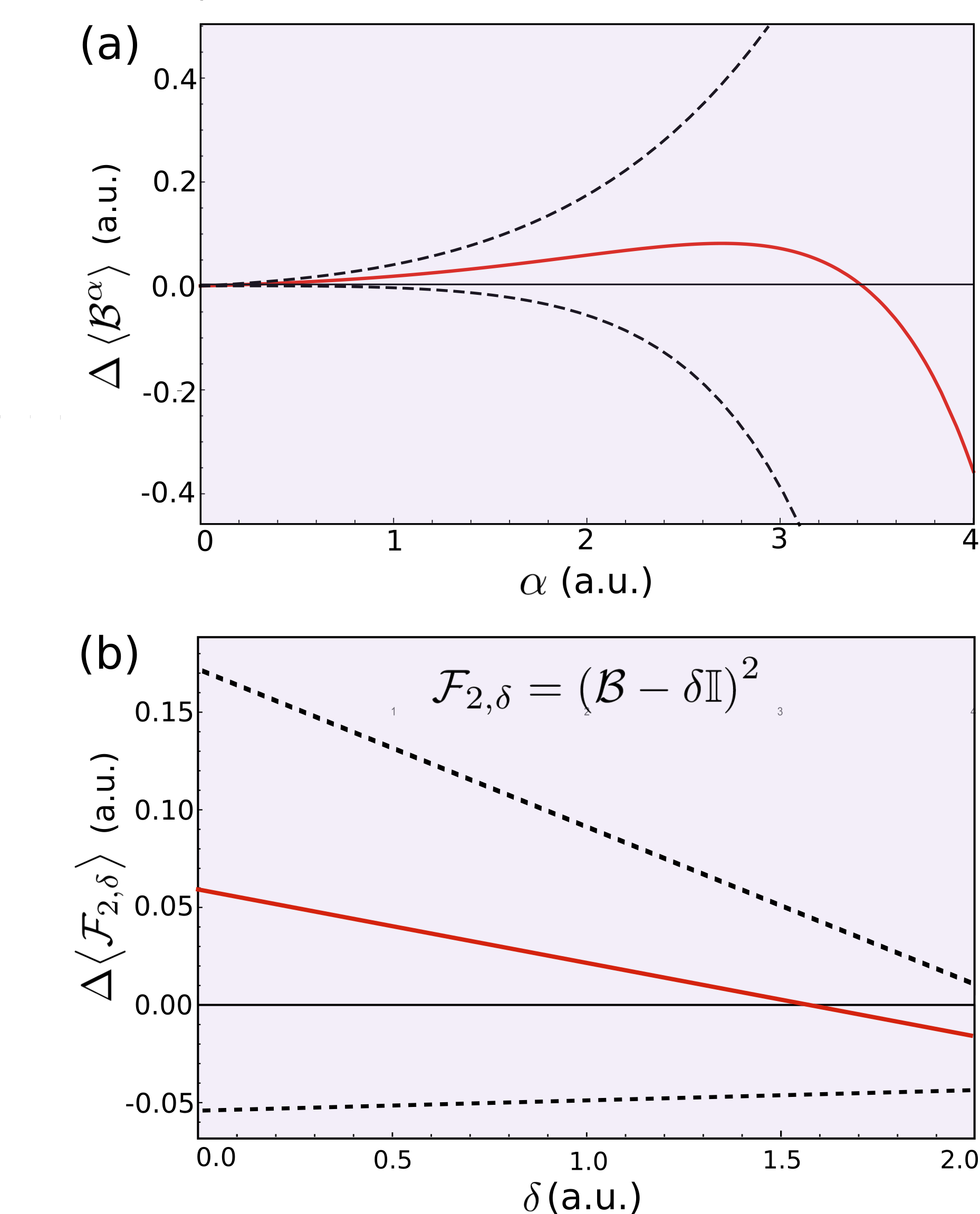
Figure S1: Additional heat leak tests using the experimental data of the Melbourne processor. None of these tests yields unambiguous detection of the heat leak.

Fig. S2 depicts heat leak tests corresponding to the Essex processor. Figure S2(a) shows the result of the test $\Delta\left\langle\mathcal{F}_{5,\delta}^{(def)}\right\rangle$, when the environment is decoupled. The observable $\mathcal{F}_{5,\delta}^{(def)}$ is given by $\mathcal{F}_{5,\delta}^{(def)}=(\mathcal{B}_{def}-\delta\mathbb{I})^{5}$, with $\mathcal{B}_{def}$ the deformed observable indicated in the main text. Consistently with the decoupling of the environment, $\Delta\left\langle\mathcal{F}_{5,\delta}^{(def)}\right\rangle\geq 0$. Finally, Fig. S2(b) shows that the test $\Delta\left\langle\mathcal{B}_{def}^{\alpha}\right\rangle$ yields unambiguous detection of the heat leak (when the environment is coupled) for $\alpha\gtrsim 6.8$. However, it is worth stressing that the employement of the shift $\delta$ enables detection with the smaller power $\alpha=5$, as shown in the main text. The inset indicates that if the deformation is not a applied to $\mathcal{B}$, no detection is possible for any $0\leq\alpha\leq 7$.

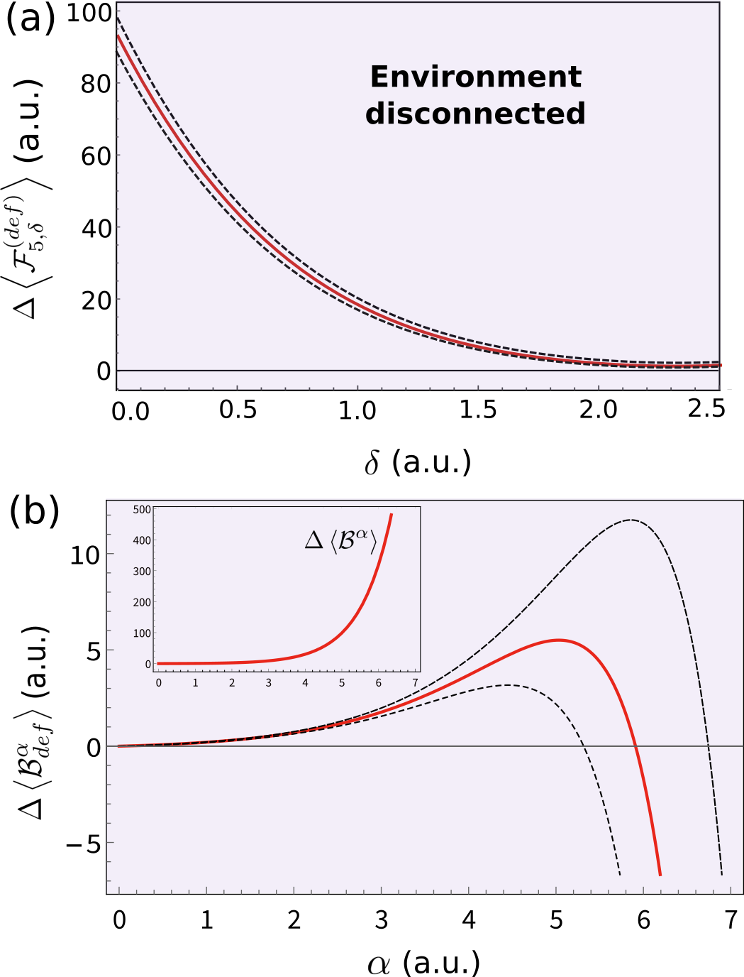
Figure S2: Additional heat leak tests using the experimental data of the Essex processor. The test in (a) is performed for the case when the environment is decoupled, and consistently yields only positive values. For the experiments with the environment coupled, the test in (b) succesfully detects the heat leak.

S-VII Comparison between environment detection using resource theory and global passivity

The framework of thermodynamic resource theory (RT) is characterized by a set of inequalities that govern the behavior of microscopic systems under thermal operations (Brandao et al., 2015). Specifically, these inequalities apply to transformations of the form

$$\rho_{s}\otimes\sigma_{c}\rightarrow\rho^{\prime}_{s}\otimes\sigma_{c}=\textrm{Tr}_{rc}U(\rho_{s}\otimes\sigma_{c}\otimes\rho_{r}^{\beta})U^{\dagger},$$ (S25)

where $\rho_{s}$ is the state of the system, $\rho_{r}^{\beta}$ is the state of a thermal bath (of arbitrary size) at inverse temperature $\beta$, $\sigma_{c}$ is the state of a catalyst, and $U$ is an energy-preserving unitary that acts globally in the aforementioned systems. Energy conservation is characterized by the condition

$$[U,H_{s}+H_{r}+H_{c}]=0,$$ (S26)

where $H_{s}$, $H_{r}$, and $H_{c}$ are respectively the Hamiltonians of the system, the bath, and the catalyst.

The RT inequalities constitute necessary and sufficient conditions on the final state of the system, $\rho^{\prime}_{s}$, in the case where both $\rho_{s}$ and $\rho^{\prime}_{s}$ commute with $H_{s}$. That is, when $\rho_{s}=\sum_{i}p_{i}^{s}|i\rangle_{s}\langle i|$ and $\rho^{\prime}_{s}=\sum_{i}p^{\prime}{}_{i}^{s}|i\rangle_{s}\langle i|$, being $|i\rangle_{s}$ eigenstates of $H_{s}$. If $q_{i}^{s}$ denote the eigenvalues of the thermal state $\rho_{s}^{\beta}=\frac{e^{-\beta H_{s}}}{Z_{s}}$, for any transformation obeying Eq. (S25) none of the “$\alpha$-free energies”

$$F_{\alpha}(\rho_{s}||\rho_{s}^{\beta})=\beta^{-1}[D_{\alpha}(\rho_{s}||\rho_{s}^{\beta})-\textrm{ln}(Z_{s})],\>-\infty<\alpha<\infty,$$ (S27)

can increase. The quantity $D_{\alpha}(\rho_{s}||\rho_{s}^{\beta})$ is the “$\alpha$-Renyi divergence”, defined as

$$D_{\alpha}(\rho_{s}||\rho_{s}^{\beta})\equiv\frac{\textrm{sgn}(\alpha)}{\alpha-1}\textrm{ln}\left(\sum_{i}\left(p_{i}^{s}\right)^{\alpha}\left(q_{i}^{s}\right)^{1-\alpha}\right).$$ (S28)

In addition, if $F_{\alpha}(\rho^{\prime}_{s}||\rho_{s}^{\beta})\leq F_{\alpha}(\rho_{s}||\rho_{s}^{\beta})$ for all $\alpha$ then there exist $\sigma_{c}$, $\rho_{r}^{\beta}$ and $U$ such that Eq. (S25) holds (Brandao et al., 2015).

Consider the initial four-qubit state prepared in the Melbourne processor. As explained in Section S-I, the closest product of thermal states $\otimes_{i=9}^{12}\rho_{i}$ is characterized by ground qubit populations $p_{0}^{(9)}=0.557$, $p_{0}^{(10)}=0.611$, $p_{0}^{(11)}=0.586$, and $p_{0}^{(12)}=0.612\sim p_{0}^{(10)}$. In this way, we can have several decompositions of the form

$$\otimes_{i=9}^{12}\rho_{i}=\rho_{s}\otimes\rho_{r}^{\beta},$$ (S29)

where $\rho_{r}^{\beta}$ is a thermal state with possible inverse temperatures $\beta=-\textrm{ln}\left(\frac{1-p_{0}^{(i)}}{p_{0}^{(i)}}\right)$, $i=9,10,11$, and $\rho_{s}$ is the state of the remaining qubits. Specifically, the role of the bath can be taken by any of the qubits, or by the bipartite system formed by qubits 10 and 12, which share the same temperature. The possible decompositions are thus

$$\otimes_{i=9}^{12}\rho_{i}=\rho_{s}\otimes\rho_{k},$$ (S30)

for $9\leq k\leq 12$, and

$$\otimes_{i=9}^{12}\rho_{i}=\rho_{s}\otimes(\rho_{10}\otimes\rho_{12}),$$ (S31)

with the state $\rho_{10}\otimes\rho_{12}$ characterized by the inverse temperature $\beta=-\textrm{ln}\left(\frac{1-p_{0}^{(10)}}{p_{0}^{(10)}}\right)$.

If $\otimes_{i=9}^{12}\rho_{i}$ evolves under a global energy-preserving unitary, any system in the decompositions (S30) and (S31) must satisfy the RT inequalities, i.e. $F_{\alpha}(\rho^{\prime}_{s}||\rho_{s}^{\beta})\leq F_{\alpha}(\rho_{s}||\rho_{s}^{\beta})$ for all $\alpha$. An example of such a unitary is provided by the circuit in Fig. S3(a), consisting of only swap gates (here $H_{i}=|1\rangle_{i}\langle 1|$ for $9\leq i\leq 12$ and therefore each swap is energy-preserving). On the other hand, suppose that first a swap takes place between an external qubit $e$, prepared in a state $\rho_{e}=\rho_{11}$ (i.e. with ground population $p_{0}^{(e)}=p_{0}^{(11)}$), and the qubit 9, as illustrated in Fig. S3(a). Since clearly this induces a non-unitary dynamics on the four-qubit system, our goal is to determine if such an interference can be detected by a violation of the form $F_{\alpha}(\rho^{\prime}_{s}||\rho_{s}^{\beta})>F_{\alpha}(\rho_{s}||\rho_{s}^{\beta})$, for some value of $\alpha$. By looking at the total final state $\otimes_{i=9}^{12}\rho^{\prime}_{i}$ we deduce that such detection is impossible. The key observation is that for any system in the decompositions (S30) or (S31), the final state $\rho^{\prime}_{s}$ is consistent with a transformation of the form (S25). Accordingly, all the $\alpha$-free energies must decrease or remain unchanged.

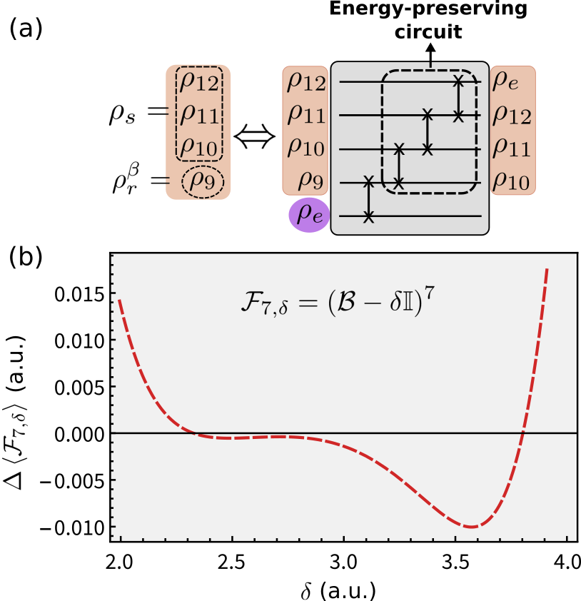
Figure S3: (a) A circuit used to check if a thermodynamic inequality of resource theory is violated due to the coupling with the environment $\rho_{e}$. The initial state $\otimes_{i=9}^{12}\rho{}_{i}$ of the total system can be decomposed into a “bath”, and a subsystem that should transform obeying the resource theory inequalities if the environment were not present. The figure illustrates a possible decomposition with the qubit 9 as bath. (b) Heat leak test $\Delta\left\langle\mathcal{F}_{7,\delta}\right\rangle$ applied to the total system. Detection of the environment is observed for $2.3\lesssim\delta\lesssim 3.8$.

The total circuit in Fig. S3(a) transforms the qubits 9-12 into the final state

$$\otimes_{i=9}^{12}\rho^{\prime}_{i}=\rho_{10}\otimes\rho_{11}\otimes\rho_{10}\otimes\rho_{11},$$ (S32)

which means that the final state for qubits 9 and 11 is $\rho_{10}$ and the final state for qubits 10 and 12 is $\rho_{11}$. For the system defined through Eqs. (S30) and (S31), the final system state corresponding to Eq. (S32) can also be obtained without the interference of the environment. Specifically, $\rho^{\prime}_{s}$ can be generated by applying suitable combinations of swaps and partial swaps between the qubits 9-12, on the initial state $\otimes_{i=9}^{12}\rho$. Given that these operations satisfy Eq. (S26) (with the identity map applied to a potential catalyst), all the RT inequalities must hold and therefore the environment cannot be detected. The operations are explicitly the following:

• If qubit 9 is the bath, Eq. (S32) implies that $\rho_{s}=\rho_{10}\otimes\rho_{11}\otimes\rho_{12}$ is transformed into $\rho^{\prime}_{s}=\rho_{11}\otimes\rho_{10}\otimes\rho_{11}$. The transformation $\rho_{10}\otimes\rho_{11}\rightarrow\rho_{11}\otimes\rho_{10}$, undergone by the qubits 10 and 11, is simply a total swap between them. Moreover, the condition $p_{0}^{(9)}<p_{0}^{(11)}<p_{0}^{(12)}$ guarantees that the transformation $\rho_{12}\rightarrow\rho_{11}$ is possible through a partial swap between the qubit 12 and the qubit 9.

• If qubit 10 is the bath, the system transforms as $\rho_{s}=\rho_{9}\otimes\rho_{11}\otimes\rho_{12}\rightarrow\rho^{\prime}_{s}=\rho_{10}\otimes\rho_{10}\otimes\rho_{11}$. The final state of the qubit 9 can be achieved by swapping it with the qubit 10. In addition, the equality $p_{0}^{(12)}=p_{0}^{(10)}$ implies that a swap between the qubits 11 and 12 yields the state $\rho_{12}\otimes\rho_{11}=\rho_{10}\otimes\rho_{11}$.

• If qubit 11 is the bath, the system transforms as $\rho_{s}=\rho_{9}\otimes\rho_{10}\otimes\rho_{12}\rightarrow\rho^{\prime}_{s}=\rho_{10}\otimes\rho_{11}\otimes\rho_{11}$. This state can be achieved in two steps. First, a swap between the qubits 9 and 10 yields $\rho_{10}\otimes\rho_{9}\otimes\rho_{12}$. Since now the qubit 10 has ground population $p_{0}^{(9)}$, it is not difficult to check that a suitable partial swap with the qubit 12 brings both qubits to the state $\rho_{11}$, thus completing the transformation.

• If qubits 10 and 12 are the bath, the system transformation $\rho_{s}=\rho_{9}\otimes\rho_{11}\rightarrow\rho^{\prime}_{s}=\rho_{10}\otimes\rho_{10}$ is achieved by simply swapping the system and the bath (recall that $\rho_{10}=\rho_{12}$).

On the other hand, Fig. S3(b) shows that $\Delta\left\langle\mathcal{F}_{7,\delta}\right\rangle<0$ for $2.3\lesssim\delta\lesssim 3.8$. This implies that GP can provide detection of a hidden environment in a situation where tests based on the RT constraints fail to detect the heat leak. Having said that, it is important to mention that global passivity refers to constraints on the total system, and not just on a subsystem as in the case of resource theory. If the total system is very large resource theory could have the advantage of requiring to evaluate its inequalities only on a small subsystem. On the other hand, we also note that in contrast to the global passivity constraints, the free energies of resource theory are not observables in the sense of representing mean values of hermitian operators. In addition, the violation of a RT inequality can reliably diagnose the presence of the environment as long as the evolution without the environment is energy-preserving. Otherwise, a violation of the RT inequalities may indicate the exchange of work, and not necessarily the existent of a heat leak.

References

Breuer and Petruccione (2002)H.-P. Breuer and F. Petruccione, Open quantum
systems (Oxford university press, 2002).
Barato and Seifert (2015)A. C. Barato and U. Seifert, Physical review letters 114, 158101 (2015).
Macieszczak et al. (2018)K. Macieszczak, K. Brandner, and J. P. Garrahan, Physical review letters 121, 130601 (2018).
Timpanaro et al. (2019)A. M. Timpanaro, G. Guarnieri, J. Goold, and G. T. Landi, Physical review
letters 123, 090604
(2019).
Gardas and Deffner (2018)B. Gardas and S. Deffner, Scientific reports 8, 1
(2018).
Buffoni and Campisi (2020)L. Buffoni and M. Campisi, Quantum Science and Technology 5, 035013 (2020).
Uzdin and Rahav (2018)R. Uzdin and S. Rahav, Physical Review
X 8, 021064 (2018).
Uzdin and Rahav (2019)R. Uzdin and S. Rahav, arXiv preprint
arXiv:1912.07922 (2019).
Huang et al. (2020)H.-Y. Huang, R. Kueng, and J. Preskill, Nature Physics 16, 1050 (2020).
Arute et al. (2019)F. Arute, K. Arya,
R. Babbush, D. Bacon, J. C. Bardin, R. Barends, R. Biswas, S. Boixo, F. G. Brandao, D. A. Buell, et al., Nature 574, 505 (2019).
Boixo et al. (2018)S. Boixo, S. V. Isakov,
V. N. Smelyanskiy,
R. Babbush, N. Ding, Z. Jiang, M. J. Bremner, J. M. Martinis, and H. Neven, Nature Physics 14, 595 (2018).
Zhong et al. (2020)H.-S. Zhong, H. Wang,
Y.-H. Deng, M.-C. Chen, L.-C. Peng, Y.-H. Luo, J. Qin, D. Wu, X. Ding, Y. Hu, et al., Science 370, 1460 (2020).
Nielsen (2002)M. A. Nielsen, Lecture Notes, Department of Physics, University of Queensland, Australia (2002).
Lindblad (2001)C. Lindblad, Non-equilibrium
entropy and irreversibility, Vol. 5 (Springer Science & Business Media, 2001).
(35)Supplemental material .
Haah et al. (2017) J. Haah, A. W. Harrow, Z. Ji, X. Wu, and N. Yu, IEEE Transactions on Information
Theory 63, 5628
(2017).
Aaronson (2019)S. Aaronson, SIAM
Journal on Computing 49, STOC18 (2019).
Paini et al. (2020)M. Paini, A. Kalev,
D. Padilha, and B. Ruck, arXiv preprint arXiv:2011.04754 (2020).
O’Donnell and Wright (2016)R. O’Donnell and J. Wright, in Proceedings of
the forty-eighth annual ACM symposium on Theory of Computing (2016) pp. 899–912.
Marshall et al. (1979)A. W. Marshall, I. Olkin, and B. C. Arnold, Inequalities: theory of majorization
and its applications, Vol. 143 (Springer, 1979).
Watrous (2018)J. Watrous, The theory of quantum
information (Cambridge University Press, 2018).
Nielsen and Chuang (2010)M. A. Nielsen and I. Chuang, Quantum computation and
quantum information (Cambridge University Press, 2010).
Cramer et al. (2010)M. Cramer, M. B. Plenio,
S. T. Flammia, R. Somma, D. Gross, S. D. Bartlett, O. Landon-Cardinal, D. Poulin, and Y.-K. Liu, Nature communications 1, 1 (2010).