Gravity and the Nonlinear Growth of Structure in the Carnegie-Spitzer-IMACS Redshift Survey

Abstract

A key obstacle to developing a satisfying theory of galaxy evolution is the difficulty in extending analytic descriptions of early structure formation into full nonlinearity, the regime in which galaxy growth occurs. Extant techniques, though powerful, are based on approximate numerical methods whose Monte Carlo-like nature hinders intuition building. Here, we develop a new solution to this problem and its empirical validation. We first derive closed-form analytic expectations for the evolution of fixed percentiles in the real-space cosmic density distribution, averaged over representative volumes observers can track cross-sectionally. Using the Lagrangian forms of the fluid equations, we show that percentiles in $\delta$—the density relative to the median—should grow as $\delta(t)\propto\delta_{0}^{\alpha}\,t^{\beta}$, where $\alpha\equiv 2$ and $\beta\equiv 2$ for Newtonian gravity at epochs after the overdensities transitioned to nonlinear growth. We then use 9.5 sq. deg. of Carnegie-Spitzer-IMACS Redshift Survey data to map galaxy environmental densities over $0.2<z<1.5$ ($\sim$7 Gyr) and infer $\alpha=1.98\pm 0.04$ and $\beta=2.01\pm 0.11$—consistent with our analytic prediction. These findings—enabled by swapping the Eulerian domain of most work on density growth for a Lagrangian approach to real-space volumetric averages—provide some of the strongest evidence that a lognormal distribution of early density fluctuations indeed decoupled from cosmic expansion to grow through gravitational accretion. They also comprise the first exact, analytic description of the nonlinear growth of structure extensible to (arbitrarily) low redshift. We hope these results open the door to new modeling of, and insight-building into, galaxy growth and its diversity in cosmological contexts.

1 Introduction

The growth of structure out of the random density fluctuations at early times is a key tenet of modern cosmology (e.g. Peebles, 1967), and the core of any theory of galaxy formation (e.g. Blumenthal et al., 1984). In Press-Schechter (Press & Schechter, 1974) and Extended Press-Schechter (Bond et al., 1991) formalisms, the growth of Fourier modes with time follows linear theory prior to decoupling from the Hubble expansion, with the addition of semi-analytical approximations for baryonic physics (e.g. Kauffmann et al., 1993; Cole et al., 1994) providing nearly all modern inferences into galaxy formation and evolution (e.g. Benson et al., 2003).

After decoupling from the Hubble expansion, however, density peaks transition from linear to non-linear growth. This nonlinear evolution of the cosmological matter density field is a difficult theoretical problem as well as an intractable observational one, owing to the impossibility of studying the time—or longitudinal—evolution of individual density fluctuations. The long-term behaviour of the matter density field in this regime has largely been trusted to $N$-body simulations, as accurate analytical methods for following the long-term trajectories of individual modes or halos have not yet been discovered. Furthermore, deriving an empirical picture of the growth of nonlinear structure requires the inversion of cross-sectional studies of distributions of different galaxies at different epochs—a fraught and perhaps underdetermined mathematical exercise. And while it has long been recognized that the growth of structure in the nonlinear regime is a difficult diffusion problem (e.g., Bond et al., 1991), the non-Markovian nature of halo growth trajectories complicates the derivation of mathematical expectations for the behaviour of mass accretion beyond those from the central limit theorem or perturbation theory (e.g., Coles & Jones, 1991; Ma & Bertschinger, 1995; Ma & Fry, 2000; Achitouv et al., 2013).

As it turns out, simple solutions to the equations governing the mean growth of density fluctuations are possible if they’re recast in terms of ensembles or percentiles in a representative distribution. Doing so conveniently shifts the fluid equations from the standard—and complicated—Eulerian framework to a simpler, Lagrangian one, allowing us to derive new analytical expectations for the mean growth of densities in the nonlinear regime. Lagrangian perturbative approaches to the growth of structure have been used for decades (e.g. Zel’dovich, 1970; Moutarde et al., 1991; Bertschinger, 1992; Bertschinger, & Jain, 1994; Bouchet, 1996) to provide insights into the topology and geometry of those first structures to collapse, as well as more accurate approximations for the rates at which structure grows while they remain attached to the Hubble expansion. In contrast to linear theory, or Lagrangian perturbation theory, our work does not begin with the assumption of $\delta\ll 1$ while linearizing the equations of motion or expanding them to higher order powers of $\delta$. Instead, we look at the mean behavior of fluctuations that have overcome the Hubble expansion by volume-averaging the equations of motion, with a specific eye towards understanding the dependence of mean growth trajectories on their initial conditions.

To validate the new analytical predictions—and the underlying picture of nonlinear growth arising from the gravitational collapse of modes that have decoupled from the Hubble expansion—we use the Carnegie-Spitzer-IMACS (CSI) Redshift Survey, a data set uniquely suited to testing this framework. CSI’s combination of broadband photometry and low-dispersion spectroscopy enabled the measurement and inference of a range of derived properties, such as redshifts, stellar masses, emission line luminosities, and information on recent star-formation. As discussed in Kelson et al. (2014) the survey was designed to study the evolution of galaxies, their environments, and the interplay between them. By selecting in the near-IR, the CSI Survey efficiently traces the stellar mass of average galaxies to $z\sim 1.5$ (and more massive ones up to $z\sim 1.8$).

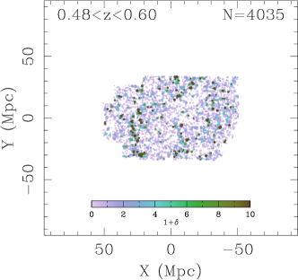
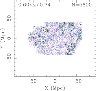
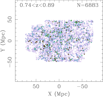
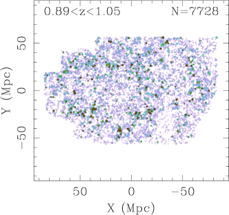
In this work we measure distributions of local stellar mass densities using CSI’s $\sim 9.5$ square degrees of coverage in the SWIRE XMM and CDFS fields. To illustrate the scale of these fields we show four redshift slices of the XMM field in Figure 1, colour coding the galaxy points by local stellar mass density (as described in §4). The CDF field, slightly smaller in area, shows visible structures that are similar in characteristic to the XMM field.

Percentiles in the distribution of local stellar mass densities—over approximately 7 Gyr of cosmic time—are used as proxies that trace the average growth of ensembles of matter density peaks. In this work we assume that local matter density fluctuations are directly traced by stellar mass (i.e. near-IR, luminous galaxies)—at least over those epochs at which galaxies exist, and thus use the evolution of density at fixed percentile to characterise the nonlinear growth of structure.

By deriving analytical expectations for how density distributions should evolve in the mean using a Lagrangian formalism, our comparisons with the CSI measurements then provide explicit tests that the growth of structure is indeed a process of gravitational collapse. Should the accuracy of the derived algebraic forms be borne out, studies of the growth of structure and the growth of galaxies may then be better understood—or even more accurately modeled—through similar analytical approaches.

The paper is structured as follows: first, we derive in §2 how ensembles of early overdensities that decoupled from the Hubble expansion should evolve on average. In §3, the CSI data set is summarized, including upgrades to the SED modeling and resulting improvements to survey robustness and data quality. In §4 we describe measuring local densities using Delaunay triangulation, followed by an empirical picture of the evolution in densities over cosmic time in §5. From the observed evolution we infer the form of the initial distrbution of densities at the time when stellar mass growth began in the universe in §6, to be used in §7 to fit for the mean growth of overdensities (and diminution of underdensities) as power-laws in both time and initial density simultaneously. Implications of our work—which confirm the analytical forms derived in §2—are summarized in §8.

The cosmological parameters used in this work are $h=0.68$, $\Omega_{M}=0.31$, and $\Omega_{\Lambda}=0.69$ (Planck Collaboration et al., 2015).

Figure 1: The positions, in comoving Mpc. for galaxies with stellar masses $M_{*}\geq 10^{10}M_{\odot}$ in four redshift slices in the CSI XMM field. The colour of each point reflects the local stellar mass density relative to the median density in the slice (see §4), while the point sizes reflect the stellar masses of the individual galaxies. High density regions are expected to grow in density contrast with time, while low density regions are expected to be hollowed out.

2 Expectations for the Growth of Structure in the Real Domain

The continuity equation dictates the evolution of individual density fluctuations with time under the constraint of mass conservation. However, the integration of the fluid equations—a procedure without closed form solutions—is only truly of astronomical utility when volume-averaged. From an astroinformatic perspective, observations cannot provide longitudinal studies of individual parcels of mass, because one observes cross sections of different density fluctuations at different epochs.

Operationally—and from the perspective of observers—this apparent shortcoming turns out to be a strength, as expectation values can be derived straightforwardly for well-defined cross-sectional studies of density fluctuations. The “trick” here is in recognizing that for regions that have decoupled from the Hubble expansion, Gauss’s theorem simplifies the continuity equation in very helpful ways when volume-averaging both sides. We note that the procedure of averaging the fluid equations—temporally or spatially—is occasionally referred to as a “Reynold’s decomposition.”

We now derive the mean Lagrangian time derivative of $\delta$, where $\delta\equiv\rho/\langle\rho\rangle-1$, for fixed percentiles in $\delta$, and where $\rho$ is the matter density at arbitrary locations within regions that have transitioned to nonlinear growth. In tracking the evolution of the distribution of local stellar mass densities, we make the assumption that stellar mass growth arises through the accretion of baryons–either in the form of gas to be converted to stars, or in the form of stars already converted from gas through previous accretion events—with the stellar baryons in either case tracking dark matter accretion in the mean. This assumption is only being made on scales much larger than that of individual galaxy-scale halos, through the summing of stellar mass over the many neighbouring vertices in the Delaunay triangulation (see below). Thus any galaxy-scale halo-mass-dependence of the efficiency with which baryons are converted to stars is averaged over many galaxies at a time.

We start with the Lagrangian continuity equation already cast in terms of overdensity $\delta$: In this approach $\delta$—normally a function of space and time—is now a function of an abstract mass-parcel coordinate, ${\mathbf{m}}$, and conformal time, $\tau\equiv t/a$:

$$\frac{D\delta({\mathbf{m}},\tau)}{D\tau}=-[1+\delta({\mathbf{m}},\tau)][\nabla\cdot{\mathbf{u}}({\mathbf{m}},\tau)]$$ (1)

and, because we are going to discuss density fluctuations that have just (barely) decoupled from the Hubble expansion, the relevant form of the momentum equation is

$$\frac{D{\mathbf{u}}({\mathbf{m}},\tau)}{D\tau}=-\nabla\phi$$ (2)

where the gravitational potential is given by

$$\nabla^{2}\phi=4\pi Ga^{2}\rho_{M}\delta({\mathbf{m}},\tau)$$ (3)

and $\rho_{M}\equiv(3\Omega_{M}H_{0}^{2})/(8\pi Ga^{3})$, the mean matter density at the epoch corresponding to scale factor $a$.

The above equations can be contrasted to those used in linear theory, and perturbation theory in general, in which one starts with the fluid equations, simplifies them assuming $\delta\ll 1$, takes the time derivative of both sides of the continuity equation, substitutes the momentum equation, and then analytically solves for the growth of modes still embedded within the Hubble expansion.

The key difference here is that while traditional approaches keep the Hubble expansion term(s), the disconnection of density fluctuations from the Hubble expansion allows one to both simplify the momentum equation as above, and, as will be shown below, somewhat trivially apply the divergence theorem. These differences between our approach and previous work obviate easy comparisons or connections. Once fluctuations have overcome the Hubble expansion, they simply do not speak to the additional “complicating” terms of the fluid equations that involve ${\dot{a}}$—and it is those terms that drive the forms of growth in, e.g., linear theory.

Even if one adopted a highly simplified “two-phase” schematic—with bubbles of matter collapsing after their disconnection from the Hubble expansion while remaining surrounded by a medium continuing that expansion and behaving according to linear theory—volume-averaged growth functions for the latter phase is not meaningful because modes grow independently and in-place. For the moment an equivalent analytical treatment of the intermediate density domain must remain an unsolved piece of the picture, as doing so remains beyond the scope of this initial work.

Using Equations 1–3, we now proceed to derive the volumetric mean change in density as functions of conformal time—$D\delta/D\tau$—at fixed initial overdensity, i.e. $\delta({\mathbf{m}},\tau_{nl})\equiv Q_{\delta}(p)$, where $p$ denotes the percentile in the distribution of initial overdensities at the onset of nonlinearity $\tau_{nl}$, $Q_{\delta}(p)$ is the quantile function of that distribution. For explicitness, we are going to use the Dirac delta function below–denoted here as $\psi$ because $\delta$ is already spoken for—to isolate specific mass parcels that originated from a set of “primordial” ones at $t=t_{nl}$, the epoch at which the relevant fluctuations hosting the seeds of galaxies detached from the Hubble expansion.

$$\left\langle\frac{D\delta}{D\tau}\right\rangle_{V|p}=\int_{V}\int_{-1}^{\infty}\frac{D\delta({\mathbf{m}},\tau)}{D\tau}\psi[\delta({\mathbf{m}},\tau_{nl})-Q_{\delta}(p)]d\delta({\mathbf{m}},\tau_{nl})dV$$ (4)

where $\psi[\delta({\mathbf{m}},\tau_{nl})-Q_{\delta}(p)]$ isolates those overdensities that start out with the same value at time $\tau=\tau_{nl}$, again, the time when the relevant density fluctuations have decoupled from the Hubble expansion. Thus,

$$\begin{split}\left\langle\frac{D\delta}{D\tau}\right\rangle_{V|p}=-\int_{V}\int_{-1}^{\infty}[1+&\delta({\mathbf{m}},\tau)][\nabla\cdot{\mathbf{u}}({\mathbf{m}},\tau)]\times\\ &\psi[\delta({\mathbf{m}},\tau_{nl})-Q_{\delta}(p)]d\delta({\mathbf{m}},\tau_{nl})dV\end{split}$$ (5)

Because modes grow independently prior to nonlinearity

$$\begin{split}\int_{V}\int_{-1}^{\infty}[\nabla\cdot{\mathbf{u}}({\mathbf{m}},\tau)]\psi[\delta({\mathbf{m}},\tau_{nl})-Q_{\delta}(p)]d\delta({\mathbf{m}},\tau_{nl})&dV\equiv\\ &\int_{V}[\nabla\cdot{\mathbf{u}}({\mathbf{m}},\tau)]dV\end{split}$$ (6)

rendering the first term in Equation 5 identically zero due to Gauss’s (divergence) theorem. Thus we are left with

$$\begin{split}\left\langle\frac{D\delta}{D\tau}\right\rangle_{V|p}=-\int_{V}&\int_{-1}^{\infty}\delta({\mathbf{m}},\tau)[\nabla\cdot{\mathbf{u}}({\mathbf{m}},\tau)]\times\\ &\psi[\delta({\mathbf{m}},\tau_{nl})-Q_{\delta}(p)]d\delta({\mathbf{m}},\tau_{nl})dV\end{split}$$ (7)

Taking the derivative of both sides with respect to $t$,

$$\begin{split}\left\langle\frac{D^{2}\delta}{D\tau^{2}}\right\rangle_{V|p}=-\frac{D}{D\tau}\int_{V}&\int_{-1}^{\infty}\delta({\mathbf{m}},\tau)[\nabla\cdot{\mathbf{u}}({\mathbf{m}},\tau)]\times\\ &\psi[\delta({\mathbf{m}},\tau_{nl})-Q_{\delta}(p)]d\delta({\mathbf{m}},\tau_{nl})dV\end{split}$$ (8)

noting that the scale factor $a$ was set at the time of decoupling. Only one of the terms in Equation 8 survives integration as nonzero, such that

$$\begin{split}\left\langle\frac{D^{2}\delta}{D\tau^{2}}\right\rangle_{V|p}=-\int_{V}\int_{-1}^{\infty}&\delta({\mathbf{m}},\tau)\biggl{[}\nabla\cdot\frac{D{\mathbf{u}}({\mathbf{m}},\tau)}{D\tau}\biggr{]}\times\\ &\psi[\delta({\mathbf{m}},\tau_{nl})-Q_{\delta}(p)]d\delta({\mathbf{m}},\tau_{nl})dV\end{split}$$ (9)

Substituting Equation 2 into the above, one obtains

$$\begin{split}\left\langle\frac{D^{2}\delta}{D\tau^{2}}\right\rangle_{V|p}=\int_{V}\int_{-1}^{\infty}\delta({\mathbf{m}},\tau)\nabla^{2}\phi\psi[\delta({\mathbf{m}},\tau_{nl})-Q_{\delta}(p)]d\delta({\mathbf{m}},\tau_{nl})dV\end{split}$$ (10)

Figure 2: Example Delaunay triangulation of CSI galaxies in the redshift slice $0.48\leq z\leq 0.60$ within the SWIRE XMM field. Each box is 7 Mpc $\times$ 7 Mpc. To compute the surface density at the location of a galaxy of interest (open orange circle) at center of each box, the areas of the adjacent triangles are summed and multipled by the depth of the redshift slice to derive a local volume element. These volume elements adapt to the point distribution uniquely. Dividing the completeness-corrected sum of the stellar masses of the galaxies at the vertices of these adjacent triangles (both blue and orange open circles) by the local volume element, one has constructed an adaptively measured local stellar mass density. Monte Carlo simulations of incomplete, but correctable, catalogs have verified that these procedures can accurately recover local densities (see text for more details)

The integration over $\delta({\mathbf{m}},\tau_{nl})$ isolates those fluctuations that began as $\delta({\mathbf{m}},\tau_{nl})=Q_{\delta}(p)\equiv\delta_{p}$, so we can write that the mean second derivative—again at fixed percentile $p$—is simply:

$$\left\langle\frac{D^{2}\delta}{D\tau^{2}}\right\rangle_{V|p}=4\pi Ga^{2}\rho_{M}\delta_{p}^{2}$$ (11)

or,

$$\left\langle\frac{D^{2}\delta}{D\tau^{2}}\right\rangle_{V|p}=\frac{3}{2}\Omega_{M}H_{0}^{2}a^{-1}\delta_{p}^{2}$$ (12)

We therefore anticipate that at times $\tau\geq\tau_{nl}$ the ensemble should appear to have a mean growth rate of

$$\left\langle\frac{D\delta}{D\tau}\right\rangle_{V|p}=\frac{3}{2}\Omega_{M}H_{0}^{2}a^{-1}\delta_{p}^{2}(\tau-\tau_{nl})$$ (13)

The constant of integration is expected to be identically zero over cosmological volumes for modes just detaching from the Hubble expansion.

Note that the above form is symmetric in $\delta_{p}$. In other words, parcels with a mass consistent with originating from the population at $\delta_{p}=-1/2$ change on average at the same rate as parcels from the $\delta_{p}=1/2$ population change on average. This is not the same thing as quantifying the amount of matter moved from the ensembles of density fluctuations defined by $p<0.5$. On average the Universe moves mass out of the population of $p<0.5$ density parcels to higher density, and we are interested in computing the amount of mass lost from the ensembles of low $\delta_{p}$in order to properly construct the cosmological evolution in the distribution of densities.

If we define $\delta^{\prime}\equiv\langle\rho\rangle/\rho-1$, the average amount of mass gained from regions of low density can be straightforwardly computed, with the chain rule recasting the result in terms of $\delta$, and yielding a result then valid for the ensembles of parcels with initial densities $\rho<\langle\rho\rangle$ (at least until the budget in material in the $p<0.5$ ensembles has been exhausted).

The two cases for the mean growth/loss trajectories at fixed density percentile are thus:

$$\left\langle\delta\right\rangle_{V|p}=\begin{cases}\delta_{p}+\frac{3}{4}\Omega_{M}H_{0}^{2}a^{-1}\delta_{p}^{2}(\tau-\tau_{nl})^{2}&\text{$\delta_{p}\geq 0$}\\ \delta_{p}-\frac{3}{4}\Omega_{M}H_{0}^{2}a^{-1}\delta_{p}^{2}(1+\delta_{p})^{2}(\tau-\tau_{nl})^{2}&\text{$\delta_{p}<0$}\end{cases}$$ (14)

where, again, $\delta_{p}\equiv\delta(p,\tau_{nl})$, and $\delta_{p}\geq-1$. When tracked through time, the density at fixed percentile should therefore follow these trajectories over epochs when sufficient material is available to sustain growth (or loss)—while none of the individual parcels of matter probably do. As a reminder, $a$ is set at the epoch of nonlinearity because the density evolution is occuring in regions that have decoupled from the Hubble expansion at that epoch; i.e., $a\equiv 1/(1+z_{nl})$.

Let us summarize the expectations derived above:

• The mean rates of growth for (initial) density fluctuations ought to be larger for regions that initially had higher density

• For density percentiles that will experience unabated collapse—e.g., $p>0.5$—density growth should scale in the mean by their initial $\delta^{\alpha}$, with $\alpha\equiv 2$;

• For density percentiles that suffer evacuation—e.g., $p<0.5$—densities should decline in the mean by their initial $\delta^{\alpha}(1+\delta)^{2}$, again $\alpha\equiv 2$;

• The mean trajectory for any density percentiles should be quadratic in time $\delta(\tau)-\delta(\tau_{nl})\propto(\tau-\tau_{nl})^{\beta}$, with $\beta\equiv 2$, at least while there is sufficient material to sustain mass flow;

• Any additional physics should manifest as additional boundary and/or initial conditions, modifying expectations from these canonical values of $\alpha\equiv 2$ and $\beta\equiv 2$

We now proceed to an explicit test of whether the evolution of the density distribution indeed follows these expectations for the growth of structure, employing a large sample of “stellar mass-selected” galaxies in CSI, to directly measure $\alpha$ and $\beta$. For ease, we will revert back to using $t$ in the remainder of the paper as we work within the framework of the CSI dataset. After studying the evolution of density percentiles in CSI, and what they mean for the mean growth of nonlinear structure, we discuss a broader set of implications for future work.

3 Summary of the Data

The Carnegie-Spitzer-IMACS Redshift Survey (Kelson et al., 2014) was designed to study the relationship between galaxy growth and environment over the last 9 Gyr of the history of the Universe, the period over which the states and appearances of today’s galaxies were defined and settled. The survey fields were targeted for low-dispersion spectroscopy with the Inamori Magellan Areal Camera and Spectrograph (IMACS; Dressler et al., 2011) using, at first, a three-layer prism described by Coil et al. (2011) for the first third of the survey, and then using an innovative eight-layer disperser for the rest. While both dispersers provide a characteristic resolution of $R\sim 25$, the newer prism more effectively balances the wavelength dependence of the spectral resolution, with higher resolution through the red. Again, details can be found in Kelson et al. (2014).

CSI chiefly selected galaxies brighter than $[3.6]\leq 21$ mag (AB). The effective stellar mass depth for a given redshift—discussed in more detail by Kelson et al. (2014)—is largely a function of the $M/L$ ratios of stellar populations, leading to approximate limits of $\sim 10^{10}M_{\odot}$ for star forming galaxies up to $z\sim 1.5$ and $\sim 3\times 10^{10}M_{\odot}$ at $z\sim 1.4$ for galaxies containing old stellar populations. The bulk of the analysis we perform is with the sample cut at $M_{*}\geq 10^{10}M_{\odot}$ when computing local stellar mass densities. When distributions of densities are computed and analysed, we perform similar analyses using cuts of $M_{*}\geq 2\times 10^{10}M_{\odot}$, $M_{*}\geq 5\times 10^{10}M_{\odot}$, and $M_{*}\geq 6\times 10^{10}M_{\odot}$ in order to test the robustness of the results.

Once the selection is a few tenths of a dex below $M^{*}$, our results do not depend sensitively to the detailed choice of how far down the mass function we compute the stellar mass densities—owing to the fact that the integral of the stellar mass function is already within $\lower 1.29167pt\hbox{$\scriptscriptstyle\;\buildrel<\over{\sim}\;$}20\%$ of convergence. When we (later) normalize local stellar mass densities by the median density at a given epoch, any systematic change with redshift in the departure from convergence is essentially removed to first order. And while variations in the shape of the stellar mass function with environment—i.e. with density—may impose a correlation in the departure from convergence with density at each epoch, this departure itself will largely evolve at the same rate as the evolution of the stellar mass function in each density percentile. As such, we should see—to first order—little-to-no systematic error in the density-dependence of the evolution of density at fixed percentile, and little-to-no systematic error in the time-dependent term of the evolution of density at fixed percentile. Furthermore, given the magnitude of the difference in $M^{*}$ between the field and the richest clusters, $<0.1$ dex at $z\sim 1$ (van der Burg et al., 2013), and the fact that such rich environments make up a tiny fraction of the volume of the universe, we expect such systematic errors to be significantly smaller than our formal/statistical errors over most of the density range being probed.

Had we counted local galaxy number densities, then these systematics would (a) be much larger, since the mass function converges very slowly in galaxy number density, and (b) the differential selection between star forming and quiescent galaxies at low stellar masses could leave a larger imprint as differential growth rates between low and high density percentiles. Furthermore, any dependencies of the rates of galaxy-galaxy merging on environment would also bias the results, whereas stellar mass is preserved under merging. In principle a comparison of number and stellar mass density evolution could provide insight into galaxy merger rates when differential selection is carefully modeled, and we leave such work for a another day.

In the SWIRE XMM field, we use a high quality set of $51\,001$ observations of $42\,251$ galaxies, and in the SWIRE CDFS field, a high quality set of $40\,680$ observations of $35\,867$ galaxies. Duplicate observations remain in our analyses, with each observation being assigned a reduced weight of $1/N_{obs}$ so that the sum of the weights for a given galaxy observed more than once would equal the weight for singly observed galaxies.

These samples have been reanalysed since the publication of Kelson et al. (2014), owing to a growing understanding that the diversity of galaxy formation histories is not only real (e.g. Abramson et al., 2016), but mathematically constrained (e.g. Kelson, 2014; Kelson et al., 2016; Dressler et al., 2018). Thus, we undertook an extensive effort to refit the CSI SEDs using a library of star formation histories generated in manner that reproduces the observed distributions of specific star formation rates of real galaxies (Kelson, 2014).

Figure 3: The results of Monte Carlo simulations of distributions of galaxies in fields of variable mean projected density on the sky, in which local projected densities are computed using the Delaunay Triangulation estimator described in the text. Here we plot local projected density estimates from catalogs suffering from source-density-dependent incompleteness in a manner similar to the CSI selection function, plotted against what the local projected densities would have been without such incompleteness. The general correspondance along the unity line indicates that the effects of slit collisions or other source-density-dependent sources of incompleteness do not systematically bias our density estimators (red points). In blue we bin the values of the true projected surface densities—showing the median and robust standard deviation of $\Sigma_{true}$— at fixed $\Sigma_{measured}$, confirming that survey incompleteness can be reliably corrected to recover the distributions of true projected densities.

Because the histories underpinning the SED fitting are better constrained, span properties that are more realistic—by definition—and have significantly fewer free parameters, we were able to recover redshifts for more objects and to fainter optical magnitudes, with an average completeness of $\sim 50\%$ over $19\ \hbox{mag}\lower 1.29167pt\hbox{$\scriptscriptstyle\;\buildrel<\over{\sim}\;$}i_{AB}\lower 1.29167pt\hbox{$\scriptscriptstyle\;\buildrel<\over{\sim}\;$}23$ mag, declining to $\sim 30\%$ at $i_{AB}\sim 24$ mag and $\sim 25\%$ at $i_{AB}\sim 24.7$ mag. As described in Kelson et al. (2014), corrections for incompleteness are trivariate functions of magnitude, colour, as well as the local density of sources in the original IRAC catalog.

In comparisons with previously published “high-resolution” redshifts (Le Fevre et al., 2003; Cooper et al., 2012; Scodeggio et al., 2018), we find that over the ranges of stellar mass and redshifts we are investigating in this paper—$M\geq 10^{10}M_{\odot}$—the CSI redshifts have typical errors of $\Delta z\approx 0.01(1+z)$ for galaxies at $0.5\leq z\leq 1.0$, and $\Delta z\approx 0.02(1+z)$ for galaxies at $1.0\leq z\leq 1.4$. The rate of catastrophic outlyers ($|\Delta z/(1+z)|>0.15$) is of order $2-3\%$—from a mixture of our own catastrophic failures and those in published redshift catalogs themselves. This level of accuracy is adequate for the analysis we propose, in which we measure local stellar mass densities in fairly wide redshift slices.

More details on the derived properties of the sample will be used in future analyses of the galaxy populations, but the work presented here relies solely on the most robust outputs of the SED fitting: redshifts and stellar masses.

Figure 4: The cumulative distributions of local stellar mass densities from the combined samples of the CSI SWIRE XMM and CDFS fields in eight redshift slices from $z=0.25$ to $z=1.4$.

4 Measuring Local Volume Densities in CSI

Here we discuss our procedure for converting galaxy point data to a map of densities, but one that is not referenced to a specific physical scale. Outside of the nonlinear regime the evolving density field is well-understood through its decomposition into Fourier modes in an Eulerian frame of reference. Typically such scales are investigated using densities measured at specific scales or wavenumbers, and counting galaxy point data in such cells has a long tradition of being used to probe the underlying distribution of matter since at least Coles & Jones (1991). But our expectations for the evolving distributions of local densities were derived specifically in a Lagrangian coordinate system, and, as such, we require densities not measured over a specific scale but be adaptive to the spatially variable structures in the galaxy distributions.

Figure 5: (a) The cumulative distributions normalized to the median density at each redshift. (b) Magnification of the low density tail of the cumulative distributions, with vertical lines at the percentiles displayed in Figure 6. (c) Same as in (b) but for the high densty tail.

Adaptive measures of local densities have been used previously to better understand how and why galaxy properties are correlated with environment, such as Dressler (1980)’s use of the radius enclosing the $10$th-nearest neighbour to define a local element of area. We opt here for a more adaptive—and computationally simple—approach, one that is not only fast but easily made robust against sources of survey incompleteness such as that arising from slit collisions or luminosity selection.

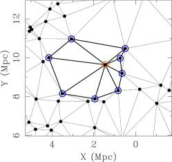
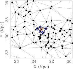
Briefly, for a list of objects in a fixed redshift slice, we run a Delaunay triangulation (part of the Visualization Toolkit; Shroeder et al., 2002). This procedure creates a unique list of triangles with galaxies at each of the vertices, but maximizes the angles to avoid particularly thin triangles. The effect of this optimization is that when circles are drawn to circumscribe the triangles, those circles contain no other points. We show three examples from the Delaunay triangulation from one redshift slice, $0.48\leq z\leq 0.60$ in the SWIRE XMM field of CSI in Figure 2. These examples span a range of local densities as can be seen from the distributions of the galaxies (black filled circles) in each 7 Mpc $\times$ 7 Mpc box, and the lighter line segments outlining the triangles.

We then compute local projected area elements at the location of a given galaxy (e.g. the galaxies circled in orange) by summing the areas of the triangles (shown in solid black) connected to that galaxy. The sizes of the triangles scale directly with the local separations of galaxies; in regions of high number density these triangles shrink commensurately. When the sum of the triangle areas is multiplied by the comoving length of the redshift slice, we have a local volume element. If we had a complete catalog containing all galaxies, we would define the density as the number of unique vertices (i.e. number of orange $+$ blue open circles) divided by that local volume element. A stellar mass density would be defined as the sum of the stellar masses of the galaxies at these vertices, divided by the local volume element.

However, no redshift survey is 100% complete and this procedure must be corrected for incompleteness. To do so we incorporate galaxy weights: each galaxy thus represents ones just like it in colour, magnitude, and local source-density but are missing from the survey. The weights are defined as the inverse of the completeness for a given galaxy’s colour, magnitude, and local source-density. Completeness-corrected local densities are thus computed by summing the weights of the galaxies and then dividing by the volume element. Completeness-corrected stellar mass densities are computed by summing the products of the weights and stellar masses of the galaxies, with subsequent division by the volume element.

As a reminder, we focus this paper on stellar mass densities because (1) the steepness of galaxy luminosity and stellar mass functions leads total number counts to converge slowly, whereas the integral of stellar mass converges much more rapidly, and (2) number counts are not preserved under galaxy-galaxy merging whereas stellar mass remains conserved (modulo tidal ejection or stripping of loosely bound stars).

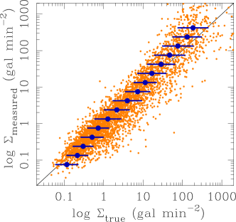
In redshift surveys such as CSI, slit collisions reduce the efficiency with which targets can be observed in regions of high source density. We demonstrate the reliability with which we could recover local number density fluctuations using Monte Carlo simulations of CSI-like survey sampling. By generating fields of galaxies with the mean CSI source density on the sky, and adding a broad range of overdensities of varying amplitudes and sizes, and then “observing” them with similar source-density dependent incompleteness to CSI, we measured local densities using our procedures and compared them to the true local densities that would have been derived from a complete and unbiased catalog.

The results of our tests are shown in Figure 3, in which the measurements of local density in the original, unculled catalog are plotted along the x-axis, while the incompleteness-corrected local number densities are plotted along the y-axis. We conclude from these simulations that so long as we measure local projected densities in CSI using redshift slices that are larger than the typical redshift uncertainties, our incompleteness-corrected local density measurements should be robust.

Figure 1 illustrates the spatial distribution of galaxies with stellar masses $M_{*}\geq 10^{10}$ M_⊙ and their local stellar mass densities within four redshift slices of $\sim 5.25$ square degrees of CSI data. The galaxy points are colour coded by local density relative to the median in each redshift slice.

The expectation—as derived in §2—is for high density regions to grow in density contrast relative to the median over time, and for the low density regions to become increasingly hollowed out. And while individual over- and under-densities cannot be tracked with lookback time, the expectation for the average behaviour of over- and under-densities can be seen visually in these data.

Qualitatively one sees a striking increase in density contrast towards late times, as the topology of the spatial distributions of the galaxies evolves—to tighter filaments and knots at later times, as well as to increasingly larger voids. Note that we do not address such evolution in the specific topological features of the galaxy distributions, but only here discuss the quantitative evolution in the global distributions of local densities.

To construct cumulative distributions of local density, we simply reorder the arrays of local densities and galaxy weights in increasing order of density, with a subsequent cumulative summation of the weight array. Normalizing the resulting array by the sum of these weights yields an array easily sifted through to identify the array positions of density percentiles. Confidence intervals are estimated with a distributional method (see Meeker, Hahn, & Escobar, 2017, and references therein) in which the probabilities that data points may be higher or lower than a given percentile are calculated using the binomial distribution.

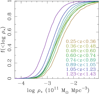
Figure 4 shows the cumulative distributions of local stellar mass densities in eight redshift slices from $z=0.25$ to $z=1.4$. A bulk increase in stellar mass density can be seen as the distributions shift towards higher mean/median values of stellar mass densities. However, for the purposes of using the distributions of local densities to characterise the nonlinear growth of structure, we want to study the distributions of normalized densities—normalized, that is, by the median in each redshift slice. These are shown in Figure 5(a), in which the distributions look qualitatively similar to each other, but are indeed distinct in their tails, as magnified in Figure 5(b) and (c).

Figure 5(b) magnifies the low density tail while Figure 5(c) magnifies the high density tail. In these plots one can directly see that from early- to late-times the high density tails evolve to increasingly larger density contrasts, and in a manner that is not identical at each density percentile. Simultaneously, the regions of low density evolve to even lower density contrasts, also by amounts that vary with percentile. In the next sections we interrogate these distributions, to determine whether these increases and decreases of density contrast with time, and their dependence on density, are consistent with the analytical forms derived in §2.

5 The Observed Distributions of Local Densities

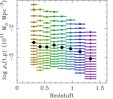
Using the local stellar mass densities, $\rho_{*}$, measured at the locations of the galaxies in CSI, we now investigate how the density distribution evolves with cosmic time. Figure 6 plots local stellar mass densities for 17 percentiles in the overall density distribution in eight redshift slices from $z\sim 0.3$ to $z\sim 1.4$, with the percentiles, $p$, defined as equivalent to the $-2\sigma$ to $+2\sigma$ for a Gaussian distribution, in intervals of $\sigma/4$. The large black circles mark the median (50th percentile) at each redshift. Cosmic variance is a significant contributor to fluctuations in the distribution with redshift. Using the MDPL2 simulation catalogs of mock galaxies (Klypin et al., 2016; Knebe et al., 2018) to estimate the magnitude of cosmic variance for CSI-like volumes, we find that the median density can fluctuate by $\sim 0.15$ dex at $z\sim 0.3$ and $\sim 0.05$ dex at $z\sim 1$.

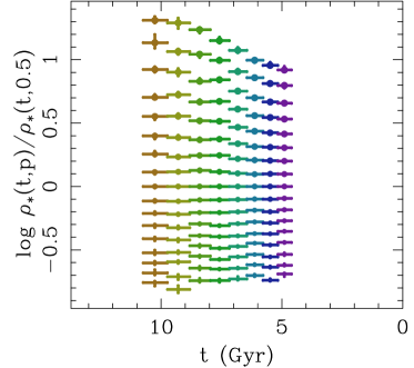
Figure 7 shows these distributions of densities relative to the median in each redshift slice. When the density percentiles are normalized relative to the median, the fluctuations due to cosmic variance are greatly diminished and typically less than 0.05 dex, with the exception of the highest percentiles ($p\lower 1.29167pt\hbox{$\scriptscriptstyle\;\buildrel>\over{\sim}\;$}0.95$) in the two lowest redshift slices shown here.

With these data alone one cannot necessarily say how individual density fluctuations grow with time in the nonlinear regime, but with these data we can measure mean rates of evolution for each percentile. As is visible in the figure, higher percentiles have densities that grow in the mean more rapidly with time than lower percentile overdensities. Underdense regions, i.e. traced by percentiles $p<0.5$, appear to show negative “growth” in the mean. Together these data will be shown below to greatly constrain the nature of the stochastic process that is the nonlinear growth of structure.

For each aspect of our analysis of the CSI redshift catalogs we have varied the widths of the redshift slices from 200 comoving Mpc to 400 comoving Mpc and find that our results remain robust, with the basic pattern shown in Figures 6 and 7. We have also performed the same analysis on catalogs of galaxies in the MDPL2 simulations (Klypin et al., 2016; Knebe et al., 2018) and find similar patterns.

Figure 6: The distribution of local stellar mass densities from the combined samples of the CSI SWIRE XMM and CDFS fields. Each point represents a fixed percentile, $p$, defined over the range $-2\sigma$ to $+2\sigma$ for a Gaussian distribution, in intervals of $\sigma/4$. The black filled circles mark the median (i.e. 50th percentile) at each redshift. Cosmic variance is expected to contribute to the scatter from one redshift to the next at a level of $\sim 0.15$ dex at $z\sim 0.3$ and $\sim 0.05$ dex at $z\sim 1$, depending on the width of the redshift slice we use (calculated using mock catalogs from the MDPL2 simulations Klypin et al., 2016; Knebe et al., 2018).

6 Making Inferences from the Evolution of the Density Percentiles

In §2 we derived a set of expectations for how the local mass density attached to a given percentile in the density distribution should evolve: quadratic in time, with a quadratic dependence on the initial density for $p>0.5$, and a quartic dependence on initial density for $p<0.5$. If one knows a priori the distribution of density fluctuations transitioning to nonlinear growth that are traced by galaxies at the start of star formation, then one has the required mapping of $p\rightarrow\delta_{p}$ to begin modeling the CSI observations in Figure 7.

Figure 7: The distribution of local stellar mass densities relative to the median within a redshift slice. Relative to the median local stellar mass density, higher density percentiles are growing more rapidly than lower density percentiles.

While we expect that distribution of densities to follow something like a lognormal distribution (e.g. Coles & Jones, 1991; Wang et al., 2011) with a standard deviation of order unity, we first employ the CSI data to test and confirm these expectations—by evolving the individual density percentiles back in time to the epochs when star formation may have began (i.e. $t=t_{0}$ at $z\lower 1.29167pt\hbox{$\scriptscriptstyle\;\buildrel>\over{\sim}\;$}10$). Once the form of the initial density distribution is understood, we will then use that functional form—with any additional and required nuisance parameters to be marginalized over—in fitting a reasonable set of of percentiles simultaneously. In this section we treat and fit each percentile independently and interpret what those individual fits yield.

For a given percentile, $p$, let us write that $\rho_{*}(t,p)/\rho_{*}(t,0.5)$ evolves according to

$$\frac{\rho_{*}(t,p)}{\rho_{*}(t,0.5)}=A(p)+B(p)(t-t_{0})^{\beta}$$ (15)

where $t$ is the time since the Big Bang and $t_{0}$ is the age of the universe when stellar mass started to form. Note that we have switched from $\tau$ in §2 to the more familiar $t$ for cosmic time. By definition $A(p)$ is the $p$th percentile density at the start of stellar mass growth, and $B(p)$ is the mean rate of growth for the ensemble of those initial densities. For this exercise we treat the $A$’s and $B$’s as independent. Once we know the functional form of the initial conditions, we will be able to abstract and generalize Equation 15.

For the purposes of the figures, we adopted a power-law evolution in time with $\beta=2$ but note that similar results are found for the inferred initial density distribution had we adopted any value at least over $1\leq\beta\leq 3$—though slightly different values for the standard deviation, $\sigma$, of the lognormal would have resulted.

Figure 8: The estimated initial densities, $A(p)$, for each percentile, are shown with the black points, as derived from fitting the evolution of the densities for each percentile as separate power-law functions of time as described by Equation 15. Individual measurements of relative density from seven redshift slices are using the coloured points. A least-squares fit for the lognormal distribution of $A$ that best fits the black points was performed, shown by the red line, with $\sigma=0.82\pm 0.01$. Evolving the highly non-lognormal distribution of densities back in time to the start of galaxy growth yields a lognormal distribution of early densities to a high degree of precision and within the measurement errors, independent of our redshift binning, and independent of the assumption that $\beta=2$.

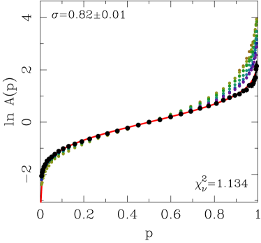
Assuming $\beta=2$, we derive a correlation of $A(p)$ with percentile, $p$, shown by the black points in Figure 8. For comparison with the individual epochs in CSI, data points for $\rho_{*}(t,p)/\rho_{*}(t,0.5)$ are also shown using the smaller coloured points (these were derived from an analysis using seven redshift slices over the same epoch, to reduce clutter). At late times, the distribution of densities is, as is well known, far from lognormality. But when we extrapolate the power-law evolution of each density percentile back to $t=t_{nl}$, we obtain a distribution of densities that is consistent with being lognormal. We performed a least-squares fit for the lognormal distribution that best represents $A(p)$, inflating the formal errors in $A(p)$ by $\sim 2.5\%$ in quadrature to account for cosmic variance (expected to be $\sim 1/10$th the redshift-to-redshift variation in the median density). To within our observational errors—reducecd $\chi^{2}=1.134$ per degree of freedom—we find that a lognormal provides an accurate description of the density distribution inferred for the epochs when star formation began, with $\sigma=0.82\pm 0.01$ (shown by the solid red line). Restated in the context of §2, $A(p)\equiv Q_{\delta}(p)+1\equiv\exp{[\sigma\Phi^{-1}(p)]}$, where $\Phi^{-1}(p)$ is the probit function and $\sigma$ is the standard deviation of the initial lognormal density distribution.

Figure 9: The correlation of $B(p)$ with $A(p)-1$ for $p\geq 0.5$, as derived from fitting the mean change in density at fixed density percentile with the power-law form of Equation 15, assuming $\beta=2$, and noting that that $\delta_{p}\equiv A(p)-1$. The expectation of $B(p)=\frac{3}{4}\Omega_{M}H_{0}^{2}(1+z_{nl})[A(p)-1]^{2}$ is shown by the black line (assuming $z_{nl}=10$). While the inferred rates of growth appear consistent with a logarithmic slope of $\alpha=2$, we fit the density- and time-dependence of the mean evolution of structure in the next section to simultaneously derive confidence intervals on $\alpha$ and $\beta$.

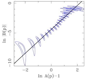
In Figure 9 we plot the measured values of $B(p)$ for positive overdensities—$p>0.5$—versus the corresponding values of $A(p)$ from the fits to the evolution of the individual percentiles. Comparing Equation 15 to the expressions derived in §2 we identify $\delta_{p}\equiv A(p)-1$, and thus plot the expectation $B(p)\propto[A(p)-1]^{2}$ by the solid black line, including the expected normalization. Note that, in general, departures in the normalization will be sensitive to the sizes of the redshift slices in our analysis and, in particular, how their sizes compare to the typical redshift uncertainties, among other systematic effects. As was clearly visible in Figure 7, regions of high density grow in the mean at rates significantly greater than regions of low density, and Figure 9 indicates that the data appear consistent with expectations of $\alpha=2$.

The accurate measurement of evolution in the low density percentiles can be hampered by incompleteness, as well as large and/or variable redshift errors, at least releative to the sizes of the redshift slices. Nonetheless, we plot in Figure 10 both the low and high density regimes from the data binning used in Figures 6 and 7. The inferred values of $A(p)$ and $B(p)$ for $p<0.5$ are shown in red, while blue is retained for $p>0.5$. As a reminder, the predicted dependence in the low density regime is $B(p)\propto[A(p)-1]^{2}A(p)^{2}$, now shown by the dashed black line. The solid black line, as in Figure 9, shows the prediction for positive overdensities. The measured evolution of both high and low density percentiles appear qualitatively consistent with the expected density-dependencies derived in §2.

We now proceed in the next section to jointly infer confidence limits on both $\alpha$ and $\beta$, adopting a lognormal form for the density distribution at the start of stellar mass growth with an unknown $\sigma$. Any quantitative constraints on $\alpha$ and $\beta$ will give us insight into the nature of the process that is the growth of structure.

7 The Mean Trajectories of Nonlinear Growth and Their Dependencies on Initial Density and Cosmic Time

In the previous section we showed that the individual density percentiles at late times can be monotonically related to equivalent percentiles in an initial lognormal spectrum of densities. We use this information now to construct a simple parameteric model for the mean growth of all the positive overdensities of the form shown in Equation 15, adopting

$$A(p)=\exp{[\sigma\Phi^{-1}(p)]}$$ (16)

$$B(p)=\begin{cases}+\gamma C[A(p)-1]^{\alpha}(t-t_{0})^{\beta}&p\geq 0.5\\ -\gamma C[A(p)-1]^{\alpha}A(p)^{2}(t-t_{0})^{\beta}&p<0.5\end{cases}$$ (17)

where $\Phi^{-1}(p)$, again, is the probit function and $\sigma$ is the standard deviation of the initial lognormal density distribution (with $\sigma$ now treated as an unknown). Our derivations in §2 predicted that these histories should be normalized by $C\equiv\frac{3}{4}\Omega_{M}H_{0}^{2}(1+z_{nl})$, but we include $\gamma$ as an of-order-unity factor in the fit to account for (a) systematics that can dilute the observed densities relative to the median; and (b) a systematic departure of the mean epoch of nonlinearity from our adoption of $z_{nl}=10$. While the zeropoint in time is set by this choice, our results are currently not sensitive to it given the lateness of the epochs being surveyed in CSI, and so marginalize over $\gamma$ as a nuisance parameter.

We grid each of the four unknowns, $\alpha$, $\beta$, $\gamma$, and $\sigma$, and compute four-dimensional posteriors. As any a priori derivation of $\sigma$ is beyond the scope of this initial work, we also marginalized over it.

Figure 10: Same as in Figure 9 but now including the low density percentiles in red. The high density expectation of $B(p)=\frac{3}{4}\Omega_{M}H_{0}^{2}(1+z_{nl})[A(p)-1]^{2}$ is shown by the solid black line, while the low density expectation of $B(p)=-\frac{3}{4}\Omega_{M}H_{0}^{2}(1+z_{nl})[A(p)-1]^{2}A(p)^{2}$ is shown using the dashed black line. While accurate measurements at low density are more hampered by systematic uncertainties in the analysis of the CSI data set compared to high density regions, the predictions and mean observed evolution for regions losing mass are in qualitative agreement. In the next section, when we fit for the density- and time-dependence of the mean evolution of structure simultaneously, we include only measurements at $\Phi^{-1}(p)\geq-1$ to mitigate the larger effects of systematic uncertainties at low density.

Figure 11: (Top) A global fit of the power-law model for the mean growth of density percentiles in CSI is shown by the blue solid lines. Dashed lines are shown at density percentiles at $\Phi^{-1}(p)<-1$, which were excluded from the fitting to mitigate against potentially larger systematic uncertainties in the measurements of low densities due to small number statistics. (Bottom) The contours for the 68% and 95% confidence intervals in $\alpha$ and $\beta$ for the fit to the binned data shown at (Top).

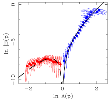
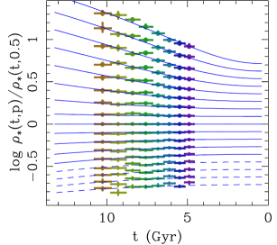
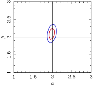
Figure 11(top) shows one set of results from fitting the evolving densities at fixed percentile, using the binned CSI data shown in Figure 7. Solid blue lines trace the best-fit model for those percentiles used in the fitting. The lowest density percentiles, expected to be systematics-dominated, were excluded from the fit and their model curves are shown using the dashed blue lines. In Figure 11(bottom), 68% and 95% contours of the joint posteriors on $\alpha$ and $\beta$ are shown, with marginalized confidence intervals of $\alpha=1.96\pm 0.04$ and $\beta=2.07\pm 0.11$ ($68\%$). These inferences for the density- and time-dependence of the mean growth of structure in the nonlinear regime do have some mild sensitivity to the details of the redshift binning and to the samples of galaxies used in the analysis.

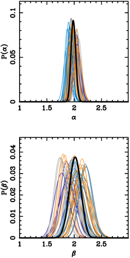
We have varied the depth of the selection, the widths of the redshift slices, as well as the maximum redshift of our study. We show marginalized posteriors for $\alpha$ and $\beta$ from $\sim 50$ such variants of our analysis of the CSI data in Figure 12. Most of these are not fully independent of each other, but the combined posteriors, shown with thick black lines, do yield a small reduction in systematics related to the redshift binning and stellar mass depth.

Using the one-dimensional posteriors in Figure 12, we derive $\alpha=1.98\pm 0.04$ and $\beta=2.01\pm 0.11$. Recall from §2—and Equation 14 in particular—that under the hypothesis that density fluctuations grow through (Newtonian) gravitational collapse, the average growth rates of ensembles of early density fluctuations should scale with the square of their initial density contrasts—an expectation now confirmed. Secondly, mean growth trajectories were predicted to be quadratic in time (again, the time since the epoch of decoupling). While the measurement uncertainties are larger for $\beta$ than for $\alpha$, the data also confirm that the mean growth trajectories follow the quadratic time dependence expected for gravitational collapse. Together, these are the first direct comparisons of observational data on these scales to fundamental predictions for nonlinear structure formation.

In the next section we discuss a few implications and side effects of our results.

8 Implications

For several decades, the most popular approaches to modeling and understanding the growth of structure have been through Monte Carlo techniques like $N$-body simulations or through the use of halo merger trees. And while such approaches offer the promise of fully self-consistent models of galaxy growth over a broad range of astronomically interesting lengthscales, both internal and external to galaxies, their richness and detail are not typically well-matched to the level of detail found in astronomical surveys. This mismatch can limit the thoroughness and ease with which one can confront data with theory, but—more importantly—it presents a substantial barrier to learning what astrophysics the data do speak to. Exactly what information is present in observations of cosmological ensembles of galaxies? The answer to this question remains elusive, as fitting semi-analytical models to observations remains an underdetermined problem (owing, e.g., to the extensive covariances between parameters; Benson, 2014),

It is within such a context that one can view recent semi-empirical approaches to galaxy formation—such as by Peng et al. (2010) and Peng et al. (2012); or Behroozi et al. (2013) and Moster et al. (2013); or Gladders et al. (2013), Oemler et al. (2013) and Abramson et al. (2016); or by Kelson (2014) and Kelson et al. (2016)—as pieces of a nascent movement to identify the essential content of observations, chiefly to uncover why some galaxies form stars more slowly or rapidly than others and at what times.

Figure 12: (Top and Bottom) The marginalized posteriors for $\alpha$ and $\beta$ in thin coloured lines from forty variants of slicing the CSI dataset, in stellar mass and redshift binning. Combining the posteriors from the different slicings of the data, we have derived a combined set of posteriors for $\alpha$ and $\beta$ shown by the thick black lines. We find that $\alpha=1.98\pm 0.04$ and $\beta=2.01\pm 0.11$, consistent with expectations for unabated gravitational collapse of early density fluctuations.

The reduction in the numbers of assumptions or parameters in such galaxy evolution frameworks ought to have helped observers glean no more than what their data could provide, but because such semi-empirical frameworks are paradigmatically distinct (see Abramson et al., 2016), they credit different—and often incompatible—physics as central to explanations for trends in the data. These incompatibilities are axiomatic, such that the concerns of one framework may even be unintelligible—literally without any associated or interpretable meaning—to the others.

And depending on whether one begins from the data—such as starting with the a priori assumption of a narrow, empirically prescribed “main sequence of star formation” on which all growing galaxies form stars as in Peng et al. (2010) until they don’t; or that there exist unique and monotonic mappings between theoretical dark matter halo accretion histories and stellar mass growth (Moster et al., 2013; Behroozi et al., 2013); or the a priori adoption of the Lilly-Madau plot (Madau et al., 1996; Lilly et al., 1996) as indicative of Hubble-timescale life cycles of galaxies as in Gladders et al. (2013) or Abramson et al. (2016); or whether one begins with a priori assumptions that the physical process of stellar mass growth is simply a stochastic process (Kelson, 2014; Kelson et al., 2016)—each conceptual framework yields strong qualitative and quantitative statements about the life cycles of galaxies while reproducing many other aspects of galaxy-level data.

Here we attempt to explicitly bridge the gap between $N$-body simulations and those semi-empirical conceptual—analytical—frameworks. By recognizing that astronomers are in the business of measuring differences between different cosmologically representative volumes observed at different epochs, we hold—operationally—that our data sets most accurately reflect volume averages of the complex, nonlinear dynamics that undergird the evolving density field (in the real universe as well as in cosmological simulations). Upon volume averaging the fluid equations, we obtained relatively simple analytical expressions for the expected growth of early density fluctuations—expressions confirmed by measurements of the distributions of local densities in CSI over 7 Gyr of history.

With exact analytical prescriptions for the average growth of those density fluctuations transitioning to nonlinearity at the start of star formation in hand, we can next ask how baryons follow or break from these expectations, and how galaxy number counts follow or break from these expectations, to begin the work of asking why (and in which kinds of density fluctuations) fewer and fewer baryons are turned into stars after $z\sim 2$, i.e. why and where the Lilly-Madau plot turns over.

This new analytical approach to the growth of structure appears to have promise as a new conceptual framework for modeling the galaxy in a statistical mechanical sense. That the MDPL2 simulations (Klypin et al., 2016; Knebe et al., 2018) show similar trends implies, too, that the catalogs of objects being produced by $N$-body simulations reflect the physical processes encoded by the fluid equations and (Newtonian) gravity (as they should). So while simulations ought to continue providing detailed ramifications of physics on small—galaxy-level—scales, this new work suggests that a volume-averaged analytical approach—encapsulating the general climate in which galaxies grow—should be seen as mathematically complementary to Monte Carlo methodologies, while being potentially better matched operationally to astronomical survey data.

However, if these results are seen stricly as a positive endorsement for standard approaches to the growth of structure, a set of stark warnings lie beneath the surface. Because another lens with which to view these results is through the language of the growth of structure as a horrible diffusion problem, though one where the particles do not experience stochastic changes to their (growth) trajectories like those in an ideal gas. If growth trajectories were like particle trajectories in an ideal gas, changes to accretion rates would be truly random, and mean growth rates, $\langle D\delta/Dt\rangle$ would scale with $t^{1/2}$. Under such a scenario growth of density fluctuations would be “Brownian,” or “Markovian,” another way of saying that changes to accretion rates at a given time are always, and everywhere, independent of previous ones.

But during nonlinear gravitational collapse, galaxies and halos—all matter density fluctuations—interact with each other, imposing what may be called “long-range dependence” on each others’ growth trajectories by some, or $1/f$ noise by many others. The gravitational interaction between density fluctuations then occurs on all timescales, meaning that changes to accretion rates become correlated with previous changes, always and everywhere. The more (and longer) the particles interact with each other, the more the mean accretion rate, $\langle D\delta/Dt\rangle$, grows faster than $t^{1/2}$ through positive reinforcement. The result is that a process of matter accretion scales as $t^{H}$ where $H$ is known as the “Hurst parameter.”

In §2 we derived $\langle D\delta/Dt\rangle\propto t$, implying that the growth of structure acts like a nonnegative stochastic process with $H=1$ (or a process with a $1/f$ noise spectrum identically). Intriguingly, this is the same kind of process that was identified at the galaxy level by studying the main sequence of star formation and the stellar mass function (e.g. Kelson et al., 2016), which both behave as if they were governed by a process with $H=1$.

An important implication immediately follows; quoting Mandelbrot & van Ness (1968), about the properties of a stochastic process $X(t,\ldots)$:

In analyzing time series $X(t,\ldots)$… it is customary to search for a decomposition into a “linear trend component” and an “oscillatory component.” The former usually … is interpreted as due to major “causal” changes in the mechanism generating $X(t,\ldots)$. The latter, on the contrary, is taken to be an “uncontrollable” stationary process, hopefully free of low-frequency components.

It is obvious that, in the case of [$\ldots$] $H\neq 1/2$, difficult statistical problems are raised by the task of distinguishing the linear trend $\Delta t$ from the nonlinear “trends” just described.

That is, when $H>1/2$, the noise itself—and long-term correlations in the noise—imposes long-term trends through (positive) reinforcement. In the case of nonlinear structure formation, gravity—and gravity alone—provides that reinforcement. Mandelbrot & van Ness (1968) end the above passage by stating that such stochastic processes fall “outside the usual dichotomy between causal trends and random perturbations.” Stated even more directly: standard tools for interpreting astronomical observations of galaxy ensembles are not appropriate for extracting historical information about individual galaxies.

As observers, astronomers are used to looking for signal by smoothing over what appears to be noise. Galaxy evolution as a practised field of study has largely been an effort to trace medians (or means) of galaxy properties with redshift/time, to smooth over the deviations from those medians as if those deviations were the “uncontrollable noise.” Decades have been spent looking further into the distant past in order to continue measuring that “linear trend component”—the mean evolution of scaling relations—under the assumption that these measurements constrain fundamental laws of astrophysics in some galaxy formation theory that is both accessible and deterministic. The tools to exploit astronomical data by other—and more meaningful—means are practically non-existent, due to the fact that the “linear trend component” and “the noise” both arise from the same underlying process, and in equal measure. As a result, the development of new tools to model distributions should be seen as paramount if progress is to be made in extracting meaning from cross-sectional studies of galaxies—not from the evolution of medians of the data, but from the “uncontrollable noise” that itself is the signal.

Until now, however, no path to generating accurate models of the nonlinear growth of structure—outside of $N$-body simulations—had seemed possible. But by shifting from an Eulerian coordinate system for the growth of structure, to a Lagrangian one, we have begun assembling an analytical framework for galaxy formation that more closely aligns with the cross-sectional nature of astronomical studies—for the evolving density field, as well as for the distinct objects that are observed at late times ($z\lower 1.29167pt\hbox{$\scriptscriptstyle\;\buildrel<\over{\sim}\;$}10$). By doing so, we aim to explicitly connect the early power spectrum to the evolving content of baryons and stellar mass, and in a manner connected to the growth of the objects we directly observe and study.

So it is with a sense of optimism that we look forward, to pushing this new conceptual approach to its logical end. Derivations of analytical expectations, such as those in §2 and elsewhere (Kelson, 2014; Kelson et al., 2016), should be taken as starting points for new analytical models of the macroeconomy of galaxy formation. For example, the volumetric averaging of stellar mass growth can be coupled with the diminishing supply of cool baryons, and, e.g., an ever increasing presence of entropy (see, e.g. Kelson et al., 2016), to construct ordinary differential equations for the evolution of the star formation rate density in different ensembles of early density fluctuations—different $\delta_{p}$—with predictions for galaxy ensembles, their stellar populations, or even their heavy element yields, as functions of late-time density.

Surely when this picture is complete, it will not only be a robust description of the evolving density field that feeds galaxy growth, but should provide new insights into its macroscopic galaxy content as well—with an exactitude thought only approachable through Monte Carlo techniques. More importantly though, by bypassing much of the fine-tuning of deterministic parameters that can complicate other theoretical approaches, we will have confidence that whatever is implied by such models will be an abstraction of exactly what our data have been trying to say all along.

References

- Abramson et al. (2015) Abramson, L. E., Gladders, M. D., Dressler, A., et al. 2015, ApJ, 801, L12
- Abramson et al. (2016) Abramson, L. E., Gladders, M. D., Dressler, A., et al. 2016, ApJ, 832, 7
- Achitouv et al. (2013) Achitouv, I., Rasera, Y., Sheth, R. K., & Corasaniti, P. S. 2013, Physical Review Letters, 111, 231303
- Behroozi et al. (2013) Behroozi, P. S., Wechsler, R. H., & Conroy, C. 2013, ApJ, 770, 57
- Benson et al. (2003) Benson, A. J., Bower, R. G., Frenk, C. S., et al. 2003, ApJ, 599, 38
- Benson (2014) Benson, A. J. 2014, MNRAS, 444, 2599
- Bertschinger (1992) Bertschinger, E. 1992, New Insights into the Universe, 65
- Bertschinger, & Jain (1994) Bertschinger, E., & Jain, B. 1994, ApJ, 431, 486
- Blumenthal et al. (1984) Blumenthal, G. R., Faber, S. M., Primack, J. R., & Rees, M. J. 1984, Nature, 311, 517
- Bond et al. (1991) Bond, J. R., Cole, S., Efstathiou, G., & Kaiser, N. 1991, ApJ, 379, 440
- Bouchet (1996) Bouchet, F. R. 1996, Dark Matter in the Universe, 565
- Coil et al. (2011) Coil, A. L., Blanton, M. R., Burles, S. M., et al. 2011, ApJ, 741, 8
- Cole et al. (1994) Cole, S., Aragon-Salamanca, A., Frenk, C. S., Navarro, J. F., & Zepf, S. E. 1994, MNRAS, 271, 781
- Coles & Jones (1991) Coles, P., & Jones, B. 1991, MNRAS, 248, 1
- Cooper et al. (2012) Cooper, M. C., Yan, R., Dickinson, M., et al. 2012, MNRAS, 425, 2116
- Dressler (1980) Dressler, A. 1980, ApJ, 236, 351
- Dressler et al. (2011) Dressler, A., Bigelow, B., Hare, T., et al. 2011, PASP, 123, 288
- Dressler et al. (2016) Dressler, A., Kelson, D. D., Abramson, L. E., et al. 2016, ApJ, 833, 251
- Dressler et al. (2018) Dressler, A., Kelson, D. D., & Abramson, L. E. 2018, ApJ, 869, 152
- Driver & Robotham (2010) Driver S.P. & Robotham A.S.G., 2010, MNRAS, 407, 2131
- Gladders et al. (2013) Gladders, M. D., Oemler, A., Dressler, A., et al. 2013, ApJ, 770, 64
- Kauffmann et al. (1993) Kauffmann, G., White, S. D. M., & Guiderdoni, B. 1993, MNRAS, 264, 201
- Kelson (2014) Kelson, D. D., 2014b, arXiv:1406.5191
- Kelson et al. (2014) Kelson, D. D., Williams, R. J., Dressler, A., et al. 2014a, ApJ, 783, 110
- Kelson et al. (2016) Kelson, D. D., Benson, A. J., & Abramson, L. E. 2016, arXiv:1610.06566
- Klypin et al. (2016) Klypin, A., Yepes, G., Gottlöber, S., Prada, F., & Heß, S. 2016, MNRAS, 457, 4340
- Knebe et al. (2018) Knebe, A., Stoppacher, D., Prada, F., et al. 2018, MNRAS, 474, 5206
- Le Fevre et al. (2003) Le Fevre, O., Vettolani, G., Maccagni, D., et al. 2003, Proc. SPIE, 173
- Lilly et al. (1996) Lilly, S. J., Le Fevre, O., Hammer, F., & Crampton, D. 1996, ApJ, 460, L1
- Ma & Bertschinger (1995) Ma, C.-P., & Bertschinger, E. 1995, ApJ, 455, 7
- Ma & Fry (2000) Ma, C.-P., & Fry, J. N. 2000, ApJ, 543, 503
- Madau et al. (1996) Madau, P., Ferguson, H. C., Dickinson, M. E., et al. 1996, MNRAS, 283, 1388
- Mandelbaum (2018) Mandelbaum, R. 2018, ARA&A, 56, 393
- Mandelbrot & van Ness (1968) Mandelbrot, B. B., & van Ness, J. W. 1968, SIAM Review, 10, 422
- Mandelbrot & Wallis (1969) Mandelbrot, B. B., & Wallis, J. R. 1969, Water Resources Research, 5, 228
- Meeker, Hahn, & Escobar (2017) Meeker, W. Q., Hahn, G. J., & Escobar, L. A., 2017, Statistical Intervals: A Guide for Practitioners and Researchers, John Wiley & Sons
- Moster et al. (2013) Moster, B. P., Naab, T., & White, S. D. M. 2013, MNRAS, 428, 3121
- Moutarde et al. (1991) Moutarde, F., Alimi, J.-M., Bouchet, F. R., et al. 1991, ApJ, 382, 377
- Noeske et al. (2007) Noeske, K. G., Weiner, B. J., Faber, S. M., et al. 2007, ApJ, 660, L43
- Ohta et al. (2004) Ohta, Y., Kayo, I., & Taruya, A. 2004, ApJ, 608, 647
- Oemler et al. (2013) Oemler, A., Jr., Dressler, A., Gladders, M. G., et al. 2013, ApJ, 770, 63
- Peebles (1967) Peebles, P. J. E. 1967, ApJ, 147, 859
- Peebles (1974) Peebles, P. J. E. 1974, A&A, 32, 391
- Peng et al. (2010) Peng, Y.-j., Lilly, S. J., Kovač, K., et al. 2010, ApJ, 721, 193
- Peng et al. (2012) Peng, Y.-j., Lilly, S. J., Renzini, A., & Carollo, M. 2012, ApJ, 757, 4
- Planck Collaboration et al. (2015) Planck Collaboration, Ade, P. A. R., Aghanim, N., et al. 2015, arXiv:1502.01589
- Press & Schechter (1974) Press, W. H., & Schechter, P. 1974, ApJ, 187, 425
- Scodeggio et al. (2018) Scodeggio, M., Guzzo, L., Garilli, B., et al. 2018, A&A, 609, A84
- Shroeder et al. (2002) Shroeder, W., Martin, K. and Lorensen, B. 2002,The Visualization Toolkit, 3rd Edition. Kitware Inc., New York.
- van der Burg et al. (2013) van der Burg, R. F. J., Muzzin, A., Hoekstra, H., et al. 2013, A&A, 557, A15
- Wang et al. (2011) Wang, X., Neyrinck, M., Szapudi, I., et al. 2011, ApJ, 735, 32
- Zel’dovich (1970) Zel’dovich, Y. B. 1970, A&A, 5, 84