Discontinuous phase transition in chemotactic aggregation
with density-dependent pressure

Abstract

Many small organisms such as bacteria can attract each other by depositing chemical attractants. At the same time, they exert repulsive force on each other when crowded, which can be modeled by effective pressure as an increasing function of the organisms’ density. As the chemical attraction becomes strong compared to the effective pressure, the system will undergo a phase transition from homogeneous distribution to aggregation. In this work, we describe the interplay of organisms and chemicals on a two-dimensional disk with a set of partial differential equations of the Patlak-Keller-Segel type. By analyzing its Lyapunov functional, we show that the aggregation transition occurs discontinuously, forming an aggregate near the boundary of the disk. The result can be interpreted within a thermodynamic framework by identifying the Lyapunov functional with free energy.

I Introduction

A ubiquitous collective phenomenon in microbial and insect populations is aggregation, which is helpful for finding food or defending themselves from toxic substances Shapiro (1988); Ma and Eaton (1992); Shapiro (1995); Crespi (2001); Detrain and Deneubourg (2006); Stewart and Costerton (2001); Secor et al. (2018). The organisms organize their movement by depositing and sensing chemicals, which is called chemotaxis. The canonical description of chemotactic aggregation is provided by the Patlak-Keller-Segel (PKS) model Patlak (1953); Keller and Segel (1970); Nanjundiah (1973); Childress and Percus (1981); Stevens (2000). In two dimensions, the model predicts collapse of the whole population into a single point when their total mass exceeds a certain threshold. Although qualitatively correct, the prediction is physically implausible because it says that all the mass is condensed into zero volume. To regularize this singular behavior, a variety of mechanisms have been proposed, including density-dependent pheromone deposition, population growth dynamics, and many others (see Ref. Hillen and Painter, 2009 for a review). One of the most convincing prescriptions is a mechanical one that incorporates the notion of pressure Gamba et al. (2003); Kowalczyk (2005); Kowalczyk and Szymańska (2008). According to this mechanism, the effective pressure between organisms increases as they come close to each other, so aggregation ceases when their chemotactic attraction is counterbalanced by the increased pressure. Experimentally, the pressure in a dense insect swarm is well fitted to a polynomial function, $\Pi=D_{0}\rho+D_{1}\rho^{2}/2!+\ldots$, where $\rho$ is the density of the organisms and $D_{i}$’s are constants Sinhuber and Ouellette (2017). Also from a thermodynamic perspective of active matter Wittkowski et al. (2014); Tiribocchi et al. (2015), such a phenomenological description of pressure holds an important place because it can readily be defined out of equilibrium due to its mechanical origin Takatori et al. (2014), and one may integrate it over volume to derive Helmholtz free energy by analogy to equilibrium thermodynamics Takatori and Brady (2015).

In this work, we wish to take a different route toward a thermodynamic description of chemically interacting organisms. We will consider an exact Lyapunov functional, i.e., a nonincreasing function of time Horstmann (2001), for a variant of the PKS model with density-dependent pressure Kowalczyk (2005); Kowalczyk and Szymańska (2008). It can be identified with a free-energy functional up to an overall constant because the long-time behavior of the system is described by the minimum of the Lyapunov functional Biler (1998); Calvez and Corrias (2008); Fatkullin (2013); Petrosyan and Hu (2014); Baek and Kim (2017), just as a thermodynamic equilibrium is associated with the free-energy minimum. We will show that this Lyapunov-functional approach gives a direct overview of the collective dynamics, especially when the functional is expressed in the Fourier space.

This study may also be viewed as an analysis of pattern formation in a reaction-diffusion system, about which a vast number of references are available (see Ref. Cross and Hohenberg, 1993 for a review). Our model corresponds to a multispecies reaction-diffusion system Fanelli et al. (2013); Madzvamuse et al. (2015) dealing with the interplay of organisms and chemicals. In addition, the density-dependent pressure $\Pi$ introduces nonlinear diffusion to this system Gambino et al. (2014) as we will see below in the governing equations. It is well known that a reaction-diffusion system may exhibit super- or subcritical bifurcation depending on its modeling details. One of our key research questions is whether the aggregation transition in our model is continuous, and we will answer this question by analyzing the Lyapunov functional.

In Sec. II, we introduce our model and its Lyapunov functional. After considering the simplest nontrivial example to see the qualitative picture, we move on to numerical calculations in Sec. III. We discuss the numerical results as well as a special case under radial symmetry (Sec. IV) and then summarize this work in Sec. V.

II Analysis

We consider the following PKS-typed model of chemotaxis in two dimensions:

$$\frac{\partial\rho}{\partial t} =\nabla\cdot\left(-\chi_{0}\rho\nabla c+\rho\nabla\Pi\right)$$ (1a)

$$\frac{\partial c}{\partial t} =f_{0}\rho+\nu_{0}\nabla^{2}c-g_{0}c,$$ (1b)

where $\rho$ is the density of organisms, $c$ is the density of pheromones, and $\Pi$ is effective pressure as a function of $\rho$. The density dependence of pressure will be truncated at the quadratic order, which means that

$$\Pi(\rho)=D_{0}\rho+D_{1}\rho^{2}/2!.$$ (2)

As we will see below, the quadratic term introduces coupling between modes in the simplest way. This system contains several modeling parameters: For the organisms, the tendency to follow a chemical gradient is given by $\chi_{0}$, and $D_{i}$’s control how sensitively they react to a density gradient. The second equation describes the pheromone dynamics, in which $f_{0}$ is the specific pheromone deposition rate, $\nu_{0}$ is the diffusion constant of pheromones, and $g_{0}$ is the specific pheromone degradation rate.

We are dealing with a population of organisms inside a domain $\Omega$, and the experimental timescale is assumed to be much shorter than their typical lifetime. The total mass of the organisms, $M\equiv\int_{\Omega}\rho~{}dV$, must thus be conserved, where $dV$ means volume elements. This is ensured by imposing the Neumann boundary conditions, $\left.\nabla\rho\cdot\hat{n}\right|_{\partial\Omega}=\left.\nabla c\cdot\hat{n}\right|_{\partial\Omega}=0$, where $\partial\Omega$ denotes the boundary of $\Omega$ and $\hat{n}$ is the normal vector at an arbitrary point on $\partial\Omega$. Specifically, we choose $\Omega$ as a two-dimensional disk of radius $l$ like a Petri dish, whose two-dimensional volume (or area) is $V=\pi l^{2}$. Note that the system of Eq. (1) always has a trivial homogeneous solution, $\rho=\rho_{0}$ and $c=(f_{0}/g_{0})\rho_{0}$, where $\rho_{0}\equiv M/V$.

Let us define $\kappa\equiv D_{1}/D_{0}$, $\lambda\equiv f_{0}\chi_{0}/(D_{0}\nu_{0})$, and $\tilde{c}\equiv(\chi_{0}/D_{0})c$. In Appendix A, we have shown that

$$\begin{split}W&\equiv\lambda\int dV\left(\kappa\frac{\rho^{3}}{6}+\frac{\rho^{2}}{2}-\rho\tilde{c}\right)\\ &+\int dV\left(\frac{g_{0}{\tilde{c}}^{2}}{2\nu_{0}}+\frac{|\nabla\tilde{c}|^{2}}{2}\right)\end{split}$$ (3)

is a Lyapunov functional in the sense that $dW/dt\leq 0$ (see Ref. Kowalczyk, 2005 for the original derivation of this functional). To apply a variational method, it is convenient to expand the configurations of $\rho$ and $c$ as Fourier-Bessel series Boas (2006):

$$\rho(r,\theta,t) =\rho_{0}+\sum_{\begin{subarray}{c}p=0\\ m=1\end{subarray}}^{\infty}Q_{pm}J_{p}(j^{\prime}_{pm}r/l)\cos[p(\theta-\eta_{pm})]$$ (4a)

$$c(r,\theta,t) =c_{0}+\sum_{\begin{subarray}{c}p=0\\ m=1\end{subarray}}^{\infty}R_{pm}J_{p}(j^{\prime}_{pm}r/l)\cos[p(\theta-\phi_{pm})],$$ (4b)

where $J_{p}$ is the Bessel function of the first kind and we have defined $j^{\prime}_{pm}$ as the $m$th zero of $\frac{d}{dx}J_{p}(x)=0$ to satisfy the boundary conditions. For example, $j^{\prime}_{11}\approx 1.841$, $j^{\prime}_{21}\approx 3.054$ and $j^{\prime}_{01}\approx 3.832$ are the smallest ones among all the possible cases of $p$ and $m$. Let us denote the set of time-dependent coefficients and phases as $\mathcal{S}\equiv\{c_{0},Q_{pm},R_{pm},\eta_{pm},\phi_{pm}|p=0,\ldots,\infty,m=1,\ldots,\infty\}$. Its elements change over time with decreasing $W$, and trajectory must be confined in a physical region in which both $\rho$ and $c$ are non-negative. We wish to find $\mathcal{S}$ that minimizes Eq. (3) inside the physical region, expecting that it will describe stationary behavior in the long time. The result will be compared with direction integration of Eq. (1).

If $\kappa=0$, then pressure is linearly proportional to $\rho$, and we can calculate Eq. (3) in a closed form as follows (see Appendix B):

$$\frac{W_{\text{st}}^{(\kappa=0)}}{V} = \frac{\lambda}{4}\sum_{p=0}^{\infty}\sum_{m=1}^{\infty}(1+\delta_{p0})J_{p}^{2}(j^{\prime}_{pm})\left(1-\frac{p^{2}}{j^{\prime 2}_{pm}}\right)z_{pm}$$ (5)

$$\times\left(z_{pm}-\frac{\chi_{0}}{D_{0}}\right)R_{pm}^{2}+\frac{W_{\text{hom}}}{V},$$

where the subscript “st” on the left-hand side means stationarity, i.e., $\partial\rho/\partial t=\partial c/\partial t=0$, and $W_{\text{hom}}$ is contribution from the homogeneous solution. We have also introduced in Eq. (5) a composite parameter,

$$z_{pm}\equiv\frac{\nu_{0}j^{\prime 2}_{pm}}{f_{0}l^{2}}+\frac{g_{0}}{f_{0}}.$$ (6)

Equation (6) contains $f_{0}l^{2}/\nu_{0}$, implying competition between the timescales of pheromone deposition and diffusion, and the second term is a ratio between the specific degradation and deposition rates of pheromones. Two points are clear from Eq. (5): First, the Lyapunov functional for $\kappa=0$ is exactly decomposed into contributions of separate modes. Second, each contribution is a quadratic function of $R_{pm}$’s: If $z_{pm}<\chi_{0}/D_{0}$, then the corresponding coefficient $R_{pm}$ can grow with decreasing the Lyapunov functional. When the chemotactic coupling strength gradually increases, therefore, the first excited mode is the one that has the lowest $j^{\prime}_{pm}$, which is $j^{\prime}_{11}\approx 1.841$. The relaxation timescale diverges at this point because the landscape of Eq. (5) is flat along the $R_{11}$ axis. When $z_{11}<\chi_{0}/D_{0}$, the excitation of $R_{11}$ is bounded only by the condition that both $\rho$ and $c$ must be non-negative. Thus, if we define an order parameter of aggregation as

$$A\equiv\max_{\vec{r}}\rho(\vec{r})-\min_{\vec{r}}\rho(\vec{r}),$$ (7)

then it shows a jump at the threshold. However, differently from a usual discontinuous transition, no hysteresis exists in this picture.

Figure 1: Schematic representation of $W_{\text{st}}$ under the two-mode approximation [Eq. (8)] to illustrate how aggregation transition occurs as the strength of chemotaxis grows. The color code means the value of Eq. (8) in arbitrary units. The red dots denote local minima, and we are plotting the region in which both $\rho$ and $c$ are non-negative. (a) If $\kappa=0$, then the origin is the only minimum below the transition point, and (b) when the system undergoes the transition, $R_{11}$ jumps to the maximal possible value while $R_{21}$ remains zero. (c) If $\kappa>0$, then the coupling term forms another local minimum in addition to the origin, before the homogeneous solution loses stability. (d) When the aggregation transition has occurred, $R_{21}$ may also take a nonzero value due to the coupling.

Now, we turn on $\kappa$ in Eq. (3) to introduce coupling between modes. By way of illustration, let us take the two lowest modes and calculate the Lyapunov functional for $\kappa>0$:

$$\frac{W_{\text{st}}}{V} \approx \frac{\lambda}{4}J_{1}^{2}(j^{\prime}_{11})\left(1-\frac{1}{j^{\prime 2}_{11}}\right)z_{11}\left[(1+\kappa\rho_{0})z_{11}-\frac{\chi_{0}}{D_{0}}\right]R_{11}^{2}$$ (8)

$$+ \frac{\lambda}{4}J_{2}^{2}(j^{\prime}_{21})\left(1-\frac{4}{j^{\prime 2}_{21}}\right)z_{21}\left[(1+\kappa\rho_{0})z_{21}-\frac{\chi_{0}}{D_{0}}\right]R_{21}^{2}$$

$$+ \kappa\frac{\lambda}{4}I_{112}\cos 2(\eta_{11}-\eta_{21})z_{11}^{2}z_{21}R_{11}^{2}R_{21}+\frac{W_{\text{hom}}}{V},$$

where $I_{112}\equiv\int_{0}^{1}xJ_{1}^{2}(j^{\prime}_{11}x)J_{2}(j^{\prime}_{21}x)dx\approx 0.0474258$. Equation (8) contains a combination of parameters, $(1+\kappa\rho_{0})z_{11}-\chi_{0}/D_{0}$, which crucially determines the landscape of $W_{\text{st}}$. Note that it is negatively proportional to $\lambda\equiv f_{0}\chi_{0}/(D_{0}\nu_{0})$, a ratio between chemotactic coupling strength ($f_{0}\chi_{0}$) and diffusivity ($D_{0}\nu_{0}$). The coefficient of $R_{11}^{2}$ vanishes when this combination equals zero, or equivalently, when

$$z_{11}=\frac{\chi_{0}/D_{0}}{1+\kappa\rho_{0}}.$$ (9)

This coincides with a prediction of linear stability analysis (Appendix C). To see an effect of the coupling term $\propto\kappa$, let us assume that $R_{11}>0$. As we have seen above, if $\kappa$ was zero, then $R_{21}$ could not be excited because it would only increase $W_{\text{st}}$ due to the second term on the right-hand side of Eq. (8). However, when $\kappa\neq 0$, the coupling effect may compete with the second term: If the coupling decreases $W_{\text{st}}$ enough to compensate for the second term, then $R_{21}$ will also be excited. As we include more and more modes in Eq. (8), we will see a cascade of excitation among them, which is essentially switched on by $R_{11}$.

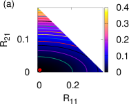
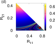
The question is then whether such coupling can render the transition continuous. The answer is negative, at least within this two-mode approximation. Let us visualize the landscape of Eq. (8). We may regard $R_{pm}$’s as positive if $p>0$, and the phase factor $\eta_{11}$ can be set to zero without loss of generality. We may also choose $\eta_{21}=\pi/2$ to make the coupling term reduce $W_{\text{st}}$ to the fullest extent. Then, $W_{\text{st}}$ becomes a function of $R_{11}$ and $R_{21}$, and its landscape can readily be depicted as in Fig. 1. Suppose $\kappa=0$ as an example: $R_{11}$ will exhibit an abrupt jump at the aggregation transition as the strength of chemotaxis grows, while $R_{21}$ remains zero [Fig. 1(a) and (b)]. Unlike a usual discontinuous transition, however, the minimum of $W^{(\kappa=0)}_{\text{st}}$ is always unique as pointed out below Eq. (7). When $\kappa\neq 0$, on the other hand, multiple local minima may coexist in the vicinity of the aggregation transition [Fig. 1(c)], although the aggregate will contain more than one wavenumbers as we see $R_{21}>0$ in Fig. 1(d). Such bistability is a characteristic feature of a discontinuous transition.

III Numerical calculation

III.1 Gradient descent

Figure 2: (a) Aggregational part of the Lyapunov functional, i.e., $W^{\text{min}}_{\text{st}}-W_{\text{hom}}$, and (b) the order parameter [Eq. (7)] as functions of $f_{0}$. As indicated by the superscript “min”, these are obtained by numerical minimization of the approximate Lyapunov functional with $P=M=3$. (c) Coefficients of the modes when aggregation has occurred, and (d) the corresponding density profile $\rho(r,\theta)$. We have set $\chi_{0}=4$ and $\rho_{0}=l=D_{0}=\nu_{0}=g_{0}=\kappa=1$ in this calculation.

To see how the above two-mode picture generalizes to a multi-mode case, we perform numerical calculation. The result confirms that the two-mode picture has already captured the essential physics of aggregation transition: Let us begin by approximating $W_{\text{st}}$ by including modes with $p<P$ and $m\leq M$ in Eq. (4). The approximate functional is then minimized by the gradient descent method with momentum,

$$\Delta\vec{w}^{\prime}=-\gamma\nabla W_{\text{st}}+\alpha\Delta\vec{w},$$ (10)

where $\vec{w}$ denotes a $(2PM)$-dimensional vector of $E_{pm}\equiv R_{pm}\cos p\phi_{pm}$ and $F_{pm}\equiv R_{pm}\sin p\phi_{pm}$, and the prime on the left-hand side means an updated quantity. We have chosen the learning rate $\gamma=10^{-5}$ and the momentum rate $\alpha=0.9$. Note that $\rho$ and $c$ may become negative in minimizing $W_{\text{st}}$, whereas the non-negativity is guaranteed by the original dynamics, Eq. (1) (see Ref. Kowalczyk, 2005 for a proof). An update of $\vec{w}$ must thus be permitted only when it keeps $\rho$ and $c$ non-negative. Specifically, we have checked the effect of updating $\vec{w}$ componentwise: A component will preserve its old value if its update violates the non-negativity condition. If no components of $\vec{w}$ can be updated under this condition, the calculation is terminated. We have also repeated this calculation with a smaller value of $\gamma$ and found consistent results. Following Ref. Baek and Kim, 2017, we set $\chi_{0}=4$ and choose other parameters, $\rho_{0}$, $l$, $D_{0}$, $\nu_{0}$, $g_{0}$, and $\kappa$, as unity. Our control parameter is the specific pheromone deposition rate $f_{0}$. According to Eq. (9), the homogeneous solution loses stability as $f_{0}$ exceeds $f_{0}^{\text{unstable}}\approx 2.195$. Although our calculation has used simple parameter values to focus on the physical mechanism, interested readers may find some of their experimental estimates for Escherichia coli in Refs. Ford et al., 1991; Saragosti et al., 2011.

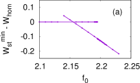
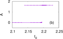
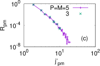
The minimization results clearly show that the system undergoes a discontinuous transition [Figs. 2(a) and 2(b)]. The two branches are obtained by starting the gradient descent algorithm from different initial conditions. The crossing point of the branches in Fig. 2(a) indicates where the transition occurs. Once $R_{11}$ becomes nonzero, the other modes also get excited [Fig. 2(c)]. However, the amplitudes are narrowly distributed, so the aggregate has compact geometry [Fig. 2(d)].

III.2 Spectral method

Figure 3: Direct simulation of Eq. (1) using the spectral method. The values of the modeling parameters are the same as in the gradient descent calculation in Fig. 2. We have chosen $P=M=3$ in Eq. (11), and the time step size for the Euler scheme is $\Delta t=10^{-3}$. (a) For each different $f_{0}$, the initial condition is set to be a uniform distribution of $\rho_{0}=1$ and $c_{0}=(f_{0}/g_{0})\rho_{0}$ with small random perturbation in the coefficients from $E_{pm}$ to $G_{pm}$. The perturbation grows for $f_{0}\gtrsim f_{0}^{\text{unstable}}\approx 2.195$. (b) For every $f_{0}$, the initial condition is a postaggregation profile, obtained from (a) by running the system for $t=50$ at $f_{0}=2.26>f_{0}^{\text{unstable}}$. The aggregate dissolves at $f_{0}\lesssim 2.15$, differently from the threshold behavior in (a), which gives a clear signal of hysteresis.

For comparison, we directly simulate Eq. (1) with the spectral method. Again, the basic idea is to expand the density fields in terms of the Fourier-Bessel modes with time-dependent coefficients as follows:

$$\begin{split}\rho^{\text{trunc}}(r,\theta,t)&=\rho_{0}+\sum_{p=0}^{P-1}\sum_{m=1}^{M}J_{p}(j^{\prime}_{pm}r/l)\\ &\times\left[E_{pm}(t)\cos(p\theta)+F_{pm}(t)\sin(p\theta)\right]\end{split}$$ (11a)

$$\begin{split}c^{\text{trunc}}(r,\theta,t)&=c_{0}(t)+\sum_{p=0}^{P-1}\sum_{m=1}^{M}J_{p}(j^{\prime}_{pm}r/l)\\ &\times\left[G_{pm}(t)\cos(p\theta)+H_{pm}(t)\sin(p\theta)\right],\end{split}$$ (11b)

where the superscript on the left-hand side means that the expansion has been truncated with certain positive integers $P$ and $M$. This representation is mathematically equivalent to Eq. (4), and it is preferable in the spectral method to work with the orthogonal basis set $\{1,J_{p}(j^{\prime}_{pm}r/l)\cos(p\theta),J_{q}(j^{\prime}_{qn}r/l)\sin(q\theta)|p=0,1,\ldots,m=1,2,\ldots,q=0,1,\ldots,n=1,2,\ldots\}$. We substitute Eq. (11) into the right-hand side of Eq. (1) and project the result onto each of the orthogonal bases to find the time derivative of each coefficient. For example, we have

$$\begin{split}\frac{dG_{pm}}{dt}&\approx\Lambda_{pm}^{-1}\int_{0}^{2\pi}d\theta\int_{0}^{l}dr~{}rJ_{p}(j^{\prime}_{pm}r/l)\cos(p\theta)\\ &\times\left(f_{0}\rho^{\text{trunc}}+\nu_{0}\nabla^{2}c^{\text{trunc}}-g_{0}c^{\text{trunc}}\right),\end{split}$$ (12)

where $\Lambda_{pm}\equiv\int_{0}^{2\pi}d\theta\int_{0}^{l}dr~{}rJ_{p}^{2}(j^{\prime}_{pm}r/l)\cos^{2}(p\theta)$ is a normalization constant. We use the Euler scheme to update the coefficients, which means that Eq. (12) is implemented as $G_{pm}(t+\Delta t)\approx G_{pm}(t)+(dG_{pm}/dt)\Delta t$ with a small step size $\Delta t$. An advantage of the spectral method is that it correctly preserves the total mass $M$, and the price is repeated numerical integration [see Eq. (12)], which we have carried out by means of the Gaussian quadrature Newman (2013).

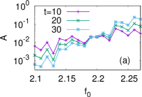
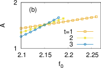
Figure 3 shows our simulation results. When we start from a uniform distribution with small perturbation, aggregation develops for $f_{0}\gtrsim f_{0}^{\text{unstable}}\approx 2.195$ [Fig. 3(a)]. On the other hand, if the simulation starts from an aggregate, then it persists even if $f_{0}$ goes below $f_{0}^{\text{unstable}}$ [Fig. 3(b)]. Such hysteresis behavior, a characteristic of discontinuous phase transition, is fully consistent with the gradient descent result of the Lyapunov functional.

IV Discussion

We have observed two points from our model: First, aggregation occurs discontinuously. It means that an aggregate forms abruptly as the chemotactic coupling strength increases, and once it happens, it will maintain itself even if the coupling weakens again. Another point is that an aggregate forms in the vicinity of the boundary. This is also plausible if we think of smaller motility near the boundary than in the middle due to the zero-flux boundary conditions. If the disk geometry is understood as a projected image of an infinite cylinder, then this picture may serve as a simple model for bacterial aggregation inside a blood vessel (see, e.g., Refs. Sittner et al., 2017; Bonazzi et al., 2018). In this context, we can see the biomedical importance of understanding the mechanism of aggregation, considering that aggregation increases antibiotic resistance structurally even without altering the innate mechanism of individual cells Stewart and Costerton (2001); Secor et al. (2018). Our result implies that a bacterial aggregate will start to form near the blood vessel wall and that it will not smoothly disappear even if the environmental condition is restored.

The two observations–the boundary effect and discontinuity–are actually related, and the transition behavior may change if we suppress aggregation at the boundary. To see this, let us restrict ourselves to a radially symmetric case ($p=0$) with $m=1$ and $2$. We have to assume $R_{01}>0$ to consider aggregation in the middle of the disk. As above, we write an approximate expression for $W_{\text{st}}$ with these two modes and check its minimum at $(R_{01}^{*},R_{02}^{*})$. When $R_{01}^{*}$ is small near the transition point, we can show that

$$R_{02}^{*}=\frac{\kappa z_{01}^{2}\int_{0}^{l}rJ_{0}^{2}(j^{\prime}_{01}r/l)J_{0}(j^{\prime}_{02}r/l)dr}{J_{0}^{2}(j^{\prime}_{02})l^{2}[(1+\kappa\rho_{0})z_{02}-\chi_{0}/D_{0}]}{R_{01}^{*}}^{2}+O\left({R_{01}^{*}}^{3}\right).$$ (13)

Because of this, the lowest-order nonvanishing term involving $R_{02}$ in $W_{\text{st}}$ is effectively of an order of $R_{01}^{4}$ around the minimum (Appendix D). If the effect of $m=2$ is negligible, then, by the same token, it can be argued that the next modes with $m>2$ will also be small compared to $m=1$. The Lyapunov functional can thus be further approximated as a cubic polynomial in $R_{01}$, as one sees in mean-field $\varphi^{3}$ theory Bender et al. (2013). The resulting phase transition is continuous, and the order parameter increases linearly with a slope $\propto\kappa^{-1}$ when the control parameter exceeds the transition threshold. It contrasts with the classical PKS model, which exhibits a discontinuous transition in two dimensions even under the restriction to $p=0$ Childress and Percus (1981) because its pressure function $\Pi$ has only logarithmic dependence on $\rho$ Kowalczyk (2005).

From a theoretical point of view, the Lyapunov-functional approach provides an intriguing way to consider free energy for active matter. We have seen that the functional greatly helps us understand the aggregation phenomenon of active particles with chemotactic interaction, just as conventional free energy does in equilibrium statistical physics. Obviously, this approach is not always applicable because most dynamical systems have no Lyapunov functional, and even if a Lyapunov functional exists, we have no systematic method to construct it. Nevertheless, it is possible to derive the functional for a class of chemotactic systems with arbitrary $\rho$ dependence of pressure as in Appendix A. For such a class of systems, the dynamics is essentially relaxational, and in this sense, they still belong to a tractable category of nonequilibrium although they deal with active matter. Finding a general form of models in this category will certainly be an interesting topic, and one may well ask, for example, whether this approach can cover recently observed effects of microswimmers such as self-organized long-ranged flows or hydrodynamically mediated interactions Mathijssen et al. (2018a, b).

By analogy between the Lyapunov functional and free energy, it would also be interesting to ask the meaning of a derivative of $W_{\text{st}}$ with respect to a system parameter, say, $f_{0}$. Figure 2(a) then implies that the derivative may serve as an alternative order parameter, showing similar behavior to that of $A$ in Fig. 2(b). One way to interpret this derivative is to note that we can produce a similar effect on the system by modulating either $f_{0}$ or $l$ [see Eq. (6)]. In other words, the system will behave in qualitatively the same way as in Fig. 2(a) when $V=\pi l^{2}$ expands. Then, one could understand $-\partial W^{\text{min}}_{\text{st}}/\partial V$ as a kind of pressure exerted on $\partial\Omega$ because pressure and volume constitute a conjugate pair in thermodynamics. Of course, this pressure is an ensemble-averaged value and should not be confused with $\Pi$. Whether it can be regarded as a physical pressure is a challenging question, which asks if the Lyapunov functional is anything more than a mere mathematical construct. Full thermodynamic understanding of this Lyapunov-functional approach is yet to be developed.

V Summary

To summarize, we have investigated a two-dimensional system of chemotactically interacting organisms which experience effective pressure as a function of their own local density. Our main analytic tool has been the Lyapunov functional, whose landscape can be seen most clearly through a mode expansion [Eq. (4) or (11)]. To couple the modes in the simplest way, we have introduced a quadratic term in the virial expansion of effective pressure. Our main interest is the transition behavior to aggregation, and we have observed clear signals of a discontinuous transition (Figs. 2 and 3). By using a two-mode approximation, we have provided a qualitative explanation for the transition behavior [Figs. 1(c) and 1(d)]. We have also discussed a special case under radial symmetry and proposed a thermodynamically motivated order parameter for aggregation transition, defined as a first-order derivative of free energy.

Appendix A Derivation of the Lyapunov functional

Let us define $\tau\equiv t/D_{0}$, $\tilde{c}\equiv(\chi_{0}/D_{0})c$, $\tilde{\Pi}(\rho)=\Pi(\rho)/D_{0}$, and $Z\equiv-\tilde{c}+\tilde{\Pi}$. The model is expressed as

$$\frac{\partial\rho}{\partial\tau} =\nabla\cdot\left(\rho\nabla Z\right)$$ (14a)

$$\frac{\chi_{0}}{\nu_{0}}\frac{\partial\tilde{c}}{\partial\tau} =\lambda\rho+\nabla^{2}\tilde{c}-\frac{g_{0}}{\nu_{0}}\tilde{c}.$$ (14b)

The total mass $M\equiv\int\rho~{}dV$ is conserved. Denoting the problem domain as $\Omega$, we impose the Neumann boundary conditions,

$$\left.\frac{\partial{\rho}}{\partial{r}}\right|_{\partial\Omega}=\left.\frac{\partial{c}}{\partial{r}}\right|_{\partial\Omega}=0.$$ (15)

We note that the following equality holds:

$$\frac{d}{d\tau}\int dVZ\rho = \int dV\rho\frac{\partial Z}{\partial\tau}+\int dVZ\frac{\partial\rho}{\partial\tau}$$ (16)

$$= \int dV\rho\frac{\partial Z}{\partial\tau}-\int dV\rho|\nabla Z|^{2}$$ (17)

because the last term on the right-hand side of Eq. (16) can be rewritten as follows:

$$\int dV\nabla\cdot(Z\rho\nabla Z)-\int dV\rho|\nabla Z|^{2} = \int dVZ\nabla\cdot(\rho\nabla Z)$$ (18)

$$= \int dVZ\frac{\partial\rho}{\partial\tau},$$ (19)

where the first term of the left-hand side of Eq. (18) is zero due to the boundary conditions. Plugging the explicit expression of $Z$ into the first term on the right-hand side of Eq. (17), we obtain

$$\frac{d}{d\tau}\int dVZ\rho=-\int dV\rho\frac{\partial\tilde{c}}{\partial\tau}+\int dV\rho\frac{\partial\tilde{\Pi}}{\partial\tau}-\int dV\rho|\nabla Z|^{2}.$$ (20)

Through integration by parts, this becomes

$$\frac{d}{d\tau}\int dV(-c^{\prime})\rho=-\int dV\rho\frac{\partial\tilde{c}}{\partial\tau}-\int dV\tilde{\Pi}\frac{\partial\rho}{\partial\tau}-\int dV\rho|\nabla Z|^{2}.$$ (21)

If we introduce $\Psi(\rho)$ such that $d\Psi/d\rho=\tilde{\Pi}$, it means

$$\frac{d}{d\tau}\int dV\left(\Psi-\rho c^{\prime}\right)=-\int dV\rho\frac{\partial\tilde{c}}{\partial\tau}-\int dV\rho|\nabla Z|^{2}.$$ (22)

To deal with the first term on the right-hand side of Eq. (22), we derive from the boundary conditions the following identity:

$$0 = \int dV\nabla\cdot\left(\frac{\partial\tilde{c}}{\partial\tau}\nabla\tilde{c}\right)$$ (23)

$$= \int dV\frac{\partial c^{\prime}}{\partial\tau}\nabla^{2}c^{\prime}+\frac{d}{d\tau}\int dV\frac{|\nabla\tilde{c}|^{2}}{2}$$ (24)

$$= \int dV\frac{\partial c^{\prime}}{\partial\tau}\left(\frac{\chi_{0}}{\nu_{0}}\frac{\partial c^{\prime}}{\partial\tau}-\lambda\rho+\frac{g_{0}}{\nu_{0}}c^{\prime}\right)+\frac{d}{d\tau}\int dV\frac{|\nabla\tilde{c}|^{2}}{2}$$ (25)

$$= \frac{\chi_{0}}{\nu_{0}}\int dV\left(\frac{\partial c^{\prime}}{\partial\tau}\right)^{2}-\lambda\int dV\rho\frac{\partial c^{\prime}}{\partial\tau}+\frac{g_{0}}{\nu_{0}}\frac{d}{d\tau}\int dV\frac{{\tilde{c}}^{2}}{2}+\frac{d}{d\tau}\int dV\frac{|\nabla\tilde{c}|^{2}}{2},$$ (26)

so that

$$\lambda\int dV\rho\frac{\partial c^{\prime}}{\partial\tau}=\frac{\chi_{0}}{\nu_{0}}\int dV\left(\frac{\partial c^{\prime}}{\partial\tau}\right)^{2}+\frac{g_{0}}{\nu_{0}}\frac{d}{d\tau}\int dV\frac{{\tilde{c}}^{2}}{2}+\frac{d}{d\tau}\int dV\frac{|\nabla\tilde{c}|^{2}}{2}.$$ (27)

By substituting Eq. (27) into Eq. (22) and rearranging the terms, we get

$$-\frac{dW}{d\tau}=\frac{\chi_{0}}{\nu_{0}}\int dV\left(\frac{\partial c^{\prime}}{\partial\tau}\right)^{2}+\lambda\int dV\rho|\nabla Z|^{2},$$ (28)

where

$$W\equiv\lambda\int dV\left(\Psi-\rho\tilde{c}\right)+\frac{g_{0}}{2\nu_{0}}\int dV{\tilde{c}}^{2}+\int dV\frac{|\nabla\tilde{c}|^{2}}{2}$$ (29)

is the Lyapunov functional in the sense that $dW/dt\leq 0$.

Appendix B Lyapunov functional for $\kappa=0$

Let us recall that the Bessel function satisfies the following equation Boas (2006):

$$\int_{0}^{1}xJ_{p}(\alpha x)J_{p}(\beta x)dx=-\frac{\alpha J_{p}(\beta)\frac{d}{dx}J_{p}(\alpha)-\beta\frac{d}{dx}J_{p}(\beta)J_{p}(\alpha)}{\alpha^{2}-\beta^{2}}$$ (30)

if $\alpha\neq\beta$. If $\alpha=j^{\prime}_{pm}$ and $\beta=j^{\prime}_{pn}$ with $m\neq n$, the right-hand side vanishes because $\frac{d}{dx}J_{p}(\alpha)=\frac{d}{dx}J_{p}(\beta)=0$. On the other hand, if $\alpha=j^{\prime}_{pm}$ and $\beta$ is an arbitrary number, then we instead have

$$\int_{0}^{1}xJ_{p}(\alpha x)J_{p}(\beta x)dx=\frac{\beta\frac{d}{dx}J_{p}(\beta)J_{p}(\alpha)}{\alpha^{2}-\beta^{2}}.$$ (31)

In the limit of $\beta\to\alpha$, we obtain

$$\int_{0}^{1}xJ_{p}(\alpha x)J_{p}(\alpha x)dx=-\frac{1}{2}J_{p}(\alpha)\frac{d^{2}}{dx^{2}}J_{p}(\alpha)$$ (32)

for $\alpha=j^{\prime}_{pm}$. We thus have the following orthogonality relation:

$$\int_{0}^{l}rJ_{p}(j^{\prime}_{pm}r/l)J_{p}(j^{\prime}_{pn}r/l)~{}dr=-\frac{l^{2}}{2}\zeta_{pm}\delta_{mn},$$ (33)

where $\delta_{mn}$ is the Kronecker $\delta$ and

$$\zeta_{pm} \equiv J_{p}(j^{\prime}_{pm})\frac{d^{2}}{dx^{2}}J_{p}(j^{\prime}_{pm})$$ (34)

$$= \frac{1}{4}J_{p}(j^{\prime}_{pm})\left[J_{p-2}(j^{\prime}_{pm})-2J_{p}(j^{\prime}_{pm})+J_{p+2}(j^{\prime}_{pm})\right]$$ (35)

$$= \frac{1}{4}J_{p}(j^{\prime}_{pm})\left[\frac{2(p-1)}{j^{\prime}_{pm}}J_{p-1}(j^{\prime}_{pm})+\frac{2(p+1)}{j^{\prime}_{pm}}J_{p+1}(j^{\prime}_{pm})-4J_{p}(j^{\prime}_{pm})\right]$$ (36)

$$= \frac{1}{4}J_{p}(j^{\prime}_{pm})\left[\frac{2(p-1)}{j^{\prime}_{pm}}\frac{p}{j^{\prime}_{pm}}J_{p}(j^{\prime}_{pm})+\frac{2(p+1)}{j^{\prime}_{pm}}\frac{p}{j^{\prime}_{pm}}J_{p}(j^{\prime}_{pm})-4J_{p}(j^{\prime}_{pm})\right]$$ (37)

$$= J_{p}^{2}(j^{\prime}_{pm})(p^{2}/j^{\prime 2}_{pm}-1).$$ (38)

From this orthogonality relation, it follows that

$$\frac{1}{\pi l^{2}}\int\rho^{2}dV = \rho_{0}^{2}-\sum_{m=1}^{\infty}\left(\zeta_{0m}Q_{0m}^{2}+\frac{1}{2}\sum_{p=1}^{\infty}\zeta_{pm}Q_{pm}^{2}\right)$$ (39)

$$\frac{1}{\pi l^{2}}\int c^{2}dV = c_{0}^{2}-\sum_{m=1}^{\infty}\left(\zeta_{0m}R_{0m}^{2}+\frac{1}{2}\sum_{p=1}^{\infty}\zeta_{pm}R_{pm}^{2}\right)$$ (40)

$$\frac{1}{\pi l^{2}}\int\rho c~{}dV = \rho_{0}c_{0}-\sum_{m=1}^{\infty}\left[\zeta_{0m}Q_{0m}R_{0m}+\frac{1}{2}\sum_{p=1}^{\infty}\zeta_{pm}Q_{pm}R_{pm}\cos p(\eta_{pm}-\phi_{pm})\right].$$ (41)

The squared gradient term can be calculated as follows:

$$\int|\nabla c|^{2}dV=\int_{-\pi}^{\pi}\int_{0}^{l}\left(\left|\frac{\partial c}{\partial r}\right|^{2}+\frac{1}{r^{2}}\left|\frac{\partial c}{\partial\theta}\right|^{2}\right)r~{}dr~{}d\theta.$$ (42)

From Eqs. (4a) and (4b), we have

$$\frac{\partial c}{\partial r} = \sum_{p=0}^{\infty}\sum_{m=1}^{\infty}\frac{j^{\prime}_{pm}}{l}\left[\left.\frac{dJ_{p}(x)}{dx}\right|_{x=j^{\prime}_{pm}r/l}\right]R_{pm}\cos p(\theta-\phi_{pm})$$ (43)

$$= \sum_{p=0}^{\infty}\sum_{m=1}^{\infty}\frac{j^{\prime}_{pm}}{l}\left[\frac{J_{p-1}(j^{\prime}_{pm}r/l)-J_{p+1}(j^{\prime}_{pm}r/l)}{2}\right]R_{pm}\cos p(\theta-\phi_{pm})$$ (44)

$$\frac{1}{r}\frac{\partial c}{\partial\theta} = \sum_{pm}J_{p}(j^{\prime}_{pm}r/l)\left(\frac{-p}{r}\right)R_{pm}\sin p(\theta-\phi_{pm})$$ (45)

$$= -\sum_{pm}\frac{j^{\prime}_{pm}}{l}\left[\frac{J_{p-1}(j^{\prime}_{pm}r/l)+J_{p+1}(j^{\prime}_{pm}r/l)}{2}\right]R_{pm}\sin p(\theta-\phi_{pm}),$$ (46)

where we have used the recurrence relations for the Bessel functions, $J_{p-1}(x)-J_{p+1}(x)=2\frac{d}{dx}J_{p}(x)$ and $J_{p-1}(x)+J_{p+1}(x)=\frac{2p}{x}J_{p}(x)$. We substitute these expressions into Eq. (42) and perform the integration. We first perform the integral over $\theta$ by using the following orthogonality:

$$\int_{-\pi}^{\pi}\cos p(\theta-\phi_{pm})\cos q(\theta-\phi_{qn})d\theta=\left\{\begin{array}[]{lcl}0&\text{~{}if~{}}&p\neq q\\ \pi\cos p(\phi_{pm}-\phi_{qn})&\text{~{}if~{}}&p=q\neq 0\\ 2\pi&\text{~{}if~{}}&p=q=0.\end{array}\right.$$ (47)

We then proceed to the integral over $r$, for which we have to evaluate the following:

$$\int|\nabla c|^{2}dV = \sum_{mn}j^{\prime}_{0m}j^{\prime}_{0n}2\pi R_{0m}R_{0n}T_{mn}$$ (48)

$$+ \sum_{p=1}^{\infty}\sum_{mn}\frac{j^{\prime}_{pm}j^{\prime}_{pn}}{2}\pi R_{pm}R_{pn}\cos p(\phi_{pm}-\phi_{pn})S_{p,mn},$$

where

$$T_{mn} \equiv l^{-2}\int_{0}^{l}dr~{}rJ_{1}(j^{\prime}_{0m}r/l)J_{1}(j^{\prime}_{0n}r/l)$$ (49)

$$S_{p,mn} \equiv l^{-2}\int_{0}^{l}dr~{}r\left[J_{p-1}(j^{\prime}_{pm}r/l)J_{p-1}(j^{\prime}_{pn}r/l)+J_{p+1}(j^{\prime}_{pm}r/l)J_{p+1}(j^{\prime}_{pn}r/l)\right].$$ (50)

The first integral is straightforward because $j^{\prime}_{0m}$’s are the zeros of $J_{1}(x)=-\frac{d}{dx}J_{0}(x)$. The standard orthogonality condition for the Bessel function gives $T_{mn}=\frac{1}{2}J_{0}^{2}(j^{\prime}_{0m})\delta_{mn}$. For $S_{p,mn}$, we use Eq. (30) together with the following recurrence relations:

$$\frac{d}{dx}J_{p-1}(x) = \frac{p-1}{x}J_{p-1}(x)-J_{p}(x)$$ (51)

$$\frac{d}{dx}J_{p+1}(x) = -\frac{p+1}{x}J_{p+1}(x)+J_{p}(x)$$ (52)

$$J_{p+1}(x) = \frac{2p}{x}J_{p}(x)-J_{p-1}(x)$$ (53)

to show

$$\int_{0}^{1}dx~{}xJ_{p-1}(\alpha x)J_{p-1}(\beta x)+\int_{0}^{1}dx~{}xJ_{p+1}(\alpha x)J_{p+1}(\beta x)$$ (54)

$$= \frac{2\alpha J_{p-1}(\beta)J_{p}(\alpha)}{\alpha^{2}-\beta^{2}}-\frac{2\beta J_{p-1}(\alpha)J_{p}(\beta)}{\alpha^{2}-\beta^{2}}-\frac{2pJ_{p}(\alpha)J_{p}(\beta)}{\alpha\beta}.$$ (55)

This is true for arbitrary $\alpha$ and $\beta$, so it implies that

$$S_{p,mn}=\frac{2j^{\prime}_{pm}J_{p-1}(j^{\prime}_{pn})J_{p}(j^{\prime}_{pm})}{j^{\prime 2}_{pm}-j^{\prime 2}_{pn}}-\frac{2j^{\prime}_{pn}J_{p-1}(j^{\prime}_{pm})J_{p}(j^{\prime}_{pn})}{j^{\prime 2}_{pm}-j^{\prime 2}_{pn}}-\frac{2pJ_{p}(j^{\prime}_{pm})J_{p}(j^{\prime}_{pn})}{j^{\prime}_{pm}j^{\prime}_{pn}}$$ (56)

for $m\neq n$. By definition, we also have $\frac{d}{dx}J_{p}(j^{\prime}_{pm})=\frac{d}{dx}J_{p}(j^{\prime}_{pn})=0$, which means that $J_{p-1}(j^{\prime}_{pm})=\frac{p}{j^{\prime}_{pm}}J_{p}(j^{\prime}_{pm})$ and $J_{p-1}(j^{\prime}_{pn})=\frac{p}{j^{\prime}_{pn}}J_{p}(j^{\prime}_{pn})$ because $\frac{d}{dx}J_{p}(x)=-\frac{p}{x}J_{p}(x)+J_{p-1}(x)$. If we plug them into Eq. (56), then we find that $S_{p,mn}$ identically vanishes for $m\neq n$. On the other hand, by taking the limit of $\beta\to\alpha$ in Eq. (55), we find

$$\int_{0}^{1}dx~{}xJ_{p-1}(\alpha x)J_{p-1}(\alpha x)+\int_{0}^{1}dx~{}xJ_{p+1}(\alpha x)J_{p+1}(\alpha x)$$ (57)

$$= \frac{1}{\alpha^{2}}\left\{(\alpha^{2}-2p)J_{p}^{2}(\alpha)+\alpha J_{p-1}(\alpha)\left[2J_{p}(\alpha)-\alpha J_{p+1}(\alpha)\right]\right\}.$$

If $\alpha=j^{\prime}_{pm}$, then this expression reduces to $\left(1-\frac{p^{2}}{\alpha^{2}}\right)J_{p}^{2}(\alpha)$ because $J_{p+1}(\alpha)=J_{p-1}(\alpha)=\frac{p}{\alpha}J_{p}(\alpha)$ from $\frac{d}{dx}J_{p}(x)=\frac{p}{x}J_{p}(x)-J_{p+1}(x)=-\frac{p}{x}J_{p}(x)+J_{p-1}(x)$. We summarize the above result as

$$S_{p,mn}=\left(1-\frac{p^{2}}{j^{\prime 2}_{pm}}\right)J_{p}^{2}(j^{\prime}_{pm})\delta_{mn}.$$ (58)

Consequently, Eq. (48) yields the following:

$$\int|\nabla c|^{2}dV=\sum_{m=1}^{\infty}\pi R_{0m}^{2}j^{\prime 2}_{0m}J_{0}^{2}(j^{\prime}_{0m})+\frac{1}{2}\sum_{p=1}^{\infty}\sum_{m=1}^{\infty}\pi R^{2}_{pm}(j^{\prime 2}_{pm}-p^{2})J_{p}^{2}(j^{\prime}_{pm}).$$ (59)

Furthermore, Eq. (1b) implies that

$$\rho_{0} =\frac{g_{0}}{f_{0}}c_{0}$$ (60a)

$$Q_{pm} =\left(\frac{\nu_{0}}{f_{0}}\frac{j^{\prime 2}_{pm}}{l^{2}}+\frac{g_{0}}{f_{0}}\right)R_{pm}=z_{pm}R_{pm}$$ (60b)

$$\eta_{pm} =\phi_{pm}$$ (60c)

in the stationary state at $t\to\infty$. By using Eqs. (39), (40), (41), (59), and (60), we obtain Eq. (5) of the main text.

Appendix C Linear stability analysis

Let us assume that the homogeneous solution is perturbed by a small amount $\epsilon$ as follows:

$$\rho(r,t) =\rho_{0}+\epsilon_{\rho}$$ (61a)

$$c(r,t) =\frac{f_{0}}{g_{0}}\rho_{0}+\epsilon_{c}.$$ (61b)

Substituting these expressions into the governing equation [Eq. (1)] and expanding the result to the first order of $\epsilon$’s, we see

$$\frac{\partial}{\partial{t}}\begin{pmatrix}\epsilon_{\rho}\\ \epsilon_{c}\\ \end{pmatrix}=\begin{pmatrix}0&0\\ f_{0}&-g_{0}\\ \end{pmatrix}\begin{pmatrix}\epsilon_{\rho}\\ \epsilon_{c}\\ \end{pmatrix}+\begin{pmatrix}D_{0}\rho_{0}+D_{1}\rho^{2}_{0}&-\chi_{0}\rho_{0}\\ 0&\nu_{0}\\ \end{pmatrix}\nabla^{2}\begin{pmatrix}\epsilon_{\rho}\\ \epsilon_{c}\\ \end{pmatrix}.$$ (62)

The solution of this linear equation is assumed to take a form of $J_{p}(kr)e^{ip\theta}e^{\eta t}$, where $J_{p}$ means the Bessel function of order $p$, and $\eta$ is the growth rate of the perturbation. The boundary conditions dictate that $(\partial/\partial r)J_{p}(kl)=0$. The lowest-wavenumber mode is given by $kl\approx 1.841$ for $p=1$. Noting that $(\nabla^{2}+k^{2})[J_{p}(kr)e^{ip\theta}]=0$, Eq. (62) reduces to the following equation for $\eta$:

$$\eta^{2}+\left[k^{2}(D_{0}\rho_{0}+D_{1}\rho^{2}_{0})+g_{0}+k^{2}\nu_{0}\right]+k^{2}(D_{0}\rho_{0}+D_{1}\rho^{2}_{0})(g_{0}+k^{2}\nu_{0}).$$ (63)

For $\eta$ to be negative, the following inequality must be met:

$$k^{2}>\left(1+\frac{D_{1}}{D_{0}}\rho_{0}\right)^{-1}\frac{f_{0}\chi_{0}}{\nu_{0}D_{0}}-\frac{g_{0}}{\nu_{0}},$$ (64)

which is the stability condition.

Appendix D Two-mode approximation under radial symmetry

When we take $\rho\approx\rho_{0}+Q_{01}J_{0}(j^{\prime}_{01}r/l)+Q_{02}J_{0}(j^{\prime}_{02}r/l)$, the corresponding Lyapunov functional becomes

$$\frac{W_{\text{st}}}{V} = \frac{W_{\text{hom}}}{V}+\frac{\lambda}{2}\sum_{m=1}^{2}J_{0}^{2}(j^{\prime}_{0m})z_{0m}\left[(1+\kappa\rho_{0})z_{0m}-\frac{\chi_{0}}{D_{0}}\right]R_{0m}^{2}$$ (65)

$$+ \frac{\kappa\lambda}{3l^{2}}\left(z_{01}^{3}R_{01}^{3}I_{111}+3z_{01}^{2}z_{02}R_{01}^{2}R_{02}I_{112}+3z_{01}z_{02}^{2}R_{01}R_{02}^{2}I_{122}+z_{02}^{3}R_{02}^{3}I_{222}\right),$$

where $I_{ijk}\equiv\int_{0}^{l}rJ_{0}(j^{\prime}_{0i}r/l)J_{0}(j^{\prime}_{0j}r/l)J_{0}(j^{\prime}_{0k}r/l)dr$. Our assumption is that $(1+\kappa\rho_{0})z_{01}-\frac{\chi_{0}}{D_{0}}<0$ and $(1+\kappa\rho_{0})z_{02}-\frac{\chi_{0}}{D_{0}}>0$ so that the homogeneous solution is instabilized by the first mode. We differentiate the above expression with respect to $R_{02}$ to find a minimum:

$$0=\left.\lambda J_{0}^{2}(j^{\prime}_{02})z_{02}R_{02}\left[(1+\kappa\rho_{0})z_{02}-\frac{\chi_{0}}{D_{0}}\right]+\frac{\kappa\lambda}{3l^{2}}(3z_{02}^{3}R_{02}^{2}I_{222}+3z_{01}^{2}z_{02}R_{01}^{2}I_{112}+6z_{01}z_{02}^{2}R_{01}R_{02}I_{122})\right|_{(R_{01}^{*},R_{02}^{*})}.$$ (66)

After solving this equation for $R_{02}^{*}$, we expand the solution as a polynomial of $R_{01}^{*}$, and the result is obtained as follows:

$$R_{02}^{*}\approx\frac{\kappa z_{01}^{2}I_{112}}{J_{0}^{2}(j^{\prime}_{02})l^{2}[(1+\kappa\rho_{0})z_{02}-\chi_{0}/D_{0}]}{R_{01}^{*}}^{2}.$$ (67)

We note that Eq. (65) does not contain $R_{02}$ and $R_{01}R_{02}$ due to the orthogonality between normal modes. Therefore, when $R_{02}\sim O\left({R_{01}}^{2}\right)$ around the minimum, the lowest contribution from $R_{02}$ is of $O\left(R_{01}^{4}\right)$.

References

- Shapiro (1988) J. A. Shapiro, Sci. Am. 258, 82 (1988).
- Ma and Eaton (1992) M. Ma and J. W. Eaton, Proc. Natl. Acad. Sci. U.S.A. 89, 7924 (1992).
- Shapiro (1995) J. A. Shapiro, BioEssays 17, 597 (1995).
- Crespi (2001) B. J. Crespi, Trends Ecol. Evol. 16, 178 (2001).
- Detrain and Deneubourg (2006) C. Detrain and J.-L. Deneubourg, Phys. Life Rev. 3, 162 (2006).
- Stewart and Costerton (2001) P. S. Stewart and J. W. Costerton, Lancet 358, 135 (2001).
- Secor et al. (2018) P. R. Secor, L. A. Michaels, A. Ratjen, L. K. Jennings, and P. K. Singh, Proc. Natl. Acad. Sci. U.S.A. 115, 10780 (2018).
- Patlak (1953) C. S. Patlak, Bull. Math. Biophys. 15, 311 (1953).
- Keller and Segel (1970) E. F. Keller and L. A. Segel, J. Theor. Biol. 26, 399 (1970).
- Nanjundiah (1973) V. Nanjundiah, J. Theor. Biol. 42, 63 (1973).
- Childress and Percus (1981) S. Childress and J. K. Percus, Math. Biosci. 56, 217 (1981).
- Stevens (2000) A. Stevens, SIAM J. Appl. Math. 61, 183 (2000).
- Hillen and Painter (2009) T. Hillen and K. J. Painter, J. Math. Biol. 58, 183 (2009).
- Gamba et al. (2003) A. Gamba, D. Ambrosi, A. Coniglio, A. de Candia, S. Di Talia, E. Giraudo, G. Serini, L. Preziosi, and F. Bussolino, Phys. Rev. Lett. 90, 118101 (2003).
- Kowalczyk (2005) R. Kowalczyk, J. Math. Anal. Appl. 305, 566 (2005).
- Kowalczyk and Szymańska (2008) R. Kowalczyk and Z. Szymańska, J. Math. Anal. Appl. 343, 379 (2008).
- Sinhuber and Ouellette (2017) M. Sinhuber and N. T. Ouellette, Phys. Rev. Lett. 119, 178003 (2017).
- Wittkowski et al. (2014) R. Wittkowski, A. Tiribocchi, J. Stenhammar, R. J. Allen, D. Marenduzzo, and M. E. Cates, Nat. Commun. 5, 4351 (2014).
- Tiribocchi et al. (2015) A. Tiribocchi, R. Wittkowski, D. Marenduzzo, and M. E. Cates, Phys. Rev. Lett. 115, 188302 (2015).
- Takatori et al. (2014) S. C. Takatori, W. Yan, and J. F. Brady, Phys. Rev. Lett. 113, 028103 (2014).
- Takatori and Brady (2015) S. C. Takatori and J. F. Brady, Phys. Rev. E 91, 032117 (2015).
- Horstmann (2001) D. Horstmann, Colloq. Math. 87, 113 (2001).
- Biler (1998) P. Biler, Adv. Math. Sci. Appl. 8, 715 (1998).
- Calvez and Corrias (2008) V. Calvez and L. Corrias, Commun. Math. Sci. 6, 417 (2008).
- Fatkullin (2013) I. Fatkullin, Nonlinearity 26, 81 (2013).
- Petrosyan and Hu (2014) K. G. Petrosyan and C.-K. Hu, Phys. Rev. E 89, 042132 (2014).
- Baek and Kim (2017) S. K. Baek and B. J. Kim, Sci. Rep. 7, 8909 (2017).
- Cross and Hohenberg (1993) M. C. Cross and P. C. Hohenberg, Rev. Mod. Phys. 65, 851 (1993).
- Fanelli et al. (2013) D. Fanelli, C. Cianci, and F. Di Patti, Eur. Phys. J. B 86, 142 (2013).
- Madzvamuse et al. (2015) A. Madzvamuse, H. S. Ndakwo, and R. Barreira, J. Math. Biol. 70, 709 (2015).
- Gambino et al. (2014) G. Gambino, M. Lombardo, and M. Sammartino, Acta Appl. Math. 132, 283 (2014).
- Boas (2006) M. L. Boas, Mathematical Methods in the Physical Sciences, 3rd ed. (Wiley, Hoboken, NJ, 2006).
- Ford et al. (1991) R. M. Ford, B. R. Phillips, J. A. Quinn, and D. A. Lauffenburger, Biotechnol. Bioeng. 37, 647 (1991).
- Saragosti et al. (2011) J. Saragosti, V. Calvez, N. Bournaveas, B. Perthame, A. Buguin, and P. Silberzan, Proc. Natl. Acad. Sci. U.S.A. 108, 16235 (2011).
- Newman (2013) M. E. J. Newman, Computational Physics (CreateSpace Independent, San Bernardino, CA, 2013).
- Sittner et al. (2017) A. Sittner, E. Bar-David, I. Glinert, A. Ben-Shmuel, S. Weiss, J. Schlomovitz, D. Kobiler, and H. Levy, PloS one 12, e0186613 (2017).
- Bonazzi et al. (2018) D. Bonazzi, V. L. Schiavo, S. Machata, I. Djafer-Cherif, P. Nivoit, V. Manriquez, H. Tanimoto, J. Husson, N. Henry, H. Chaté, et al., Cell 174, 143 (2018).
- Bender et al. (2013) C. M. Bender, B. K. Berntson, D. Parker, and E. Samuel, Am. J. Phys. 81, 173 (2013).
- Mathijssen et al. (2018a) A. J. T. M. Mathijssen, F. Guzmán-Lastra, A. Kaiser, and H. Löwen, Phys. Rev. Lett. 121, 248101 (2018a).
- Mathijssen et al. (2018b) A. J. T. M. Mathijssen, R. Jeanneret, and M. Polin, Phys. Rev. Fluids 3, 033103 (2018b).