Spooky effect in optimal OSPA estimation and how GOSPA solves it

Abstract

In this paper, we show the spooky effect at a distance that arises in optimal estimation of multiple targets with the optimal sub-pattern assignment (OSPA) metric. This effect refers to the fact that if we have several independent potential targets at distant locations, a change in the probability of existence of one of them can completely change the optimal estimation of the rest of the potential targets. As opposed to OSPA, the generalised OSPA (GOSPA) metric ($\alpha=2$) penalises localisation errors for properly detected targets, false targets and missed targets. As a consequence, optimal GOSPA estimation aims to lower the number of false and missed targets, as well as the localisation error for properly detected targets, and avoids the spooky effect.

I Introduction

Multiple target estimation is an inherent part of many applications such as surveillance, self-driving vehicles, and air-traffic control [1, 2, 3]. The special characteristic of multiple target estimation is that it requires the estimation of the number of targets, which is unknown, as well as their states.

In a Bayesian paradigm, given some noisy observations of a random variable of interest, all information about this variable is contained in its posterior probability density function [4]. Given the posterior and a cost function, optimal estimation is performed by minimising the expected value of this cost function with respect to the posterior [5, 6]. For example, for random vectors of fixed dimensionality, if the cost function is the square error, the optimal estimator, which is referred to as the minimum mean square error estimator, is the posterior mean.

In multi-target systems, the variable of interest can be represented as a set of unknown cardinality and whose elements are the target states [7]. As in systems of fixed dimensionality, developing optimal estimators for multi-target systems is important, as they use all the information in the posterior density to provide estimates with the smallest possible error. Before developing an optimal multi-target estimator, a key aspect is the choice of a cost function that measures errors in a suitable way and, therefore, yields desirable properties for the optimal multi-target estimator. In this paper, we analyse and discuss properties of optimal estimators based on multi-target metrics, which we proceed to review.

The Hausdorff metric is a general metric for sets and was proposed to be used for sets of targets in [8], but it is relatively insensitive to differences in the number of targets [8]. The Wasserstein metrics were originally used to measure the similarity between probability distributions [9, 10] and were proposed for sets of targets in [8]. However, they lack a physically consistent interpretation when the sets have different cardinalities [11]. The optimal sub-pattern assignment (OSPA) metric, which has parameters $p$ and $c$, was firstly introduced to measure the similarity between distributions of point processes [12, page 669]. The OSPA metric was proposed to be used for sets of targets in [11] and has better properties for multi-target error evaluation than Hausdorff and Wassertein metrics. The use of OSPA for optimal multiple target estimation with known number of targets has been considered in [13, 14, 15, 16, 17, 18]. With unknown number of targets, the use of unnormalised OSPA (UOSPA) for multi-target estimation was proposed in [19]. The cardinalized optimal linear assignment (COLA) metric was proposed in the context of map estimation in robotics [20]. COLA corresponds to the UOSPA metric divided by $c$, which implies that optimal estimators for COLA and UOSPA are the same.

The generalised OSPA (GOSPA) metric [21] generalises the UOSPA metric by adding a parameter $\alpha$ to adjust the cardinality mismatch penalty. Importantly, if and only if $\alpha=2$, the GOSPA metric can be written in terms of assignment sets, in which targets can be left unassigned and only nearby targets are assigned to each other [21, Proposition 1]. In this case, GOSPA decomposes into localisation errors for properly detected targets (assigned targets), costs for missed targets and costs for false targets (unassigned targets). Therefore, the GOSPA metric, contrary to OSPA and UOSPA, favours estimates that locate detected targets well and keep the number of false and missed targets to a minimum, as in traditional multiple target tracking assessment methods [22, 23, 24, 25]. For example, adding false targets to an estimate does not necessarily increase the OSPA/UOSPA error, but it always increases GOSPA error [21, Example 2].

In this work, we show that optimal mean square OSPA and UOSPA estimators produce an effect, which we refer to as spooky effect at a distance, due to a similar effect in the cardinality probability hypothesis density filter [26]. The spooky effect in optimal estimation refers to the fact that a small change in the probability of existence of one potential target can dramatically change the optimal estimation of far-away independent potential targets. This is especially significant with OSPA, as the appearance of a potential target with a small probability of existence can trigger that all potential targets in the scene are detected, even if their probabilities of existence are low. We also show that the spooky effect is absent in optimal mean square GOSPA ($\alpha=2$) estimation. In this case, the optimization problem for independent potential targets in distant regions can be separated into local problems, such that the detection of a potential targets depends only on its distribution, and not the distribution of the rest of the targets.

The rest of the paper is organised as follows. Section II reviews the considered metrics and the optimal estimation problem. The spooky effect in optimal OSPA and UOSPA metric is explained in Section III. Section III also shows that optimal GOSPA estimation does not present spooky effect. Finally, conclusions are drawn in Section IV.

II Background

In this section, we review the OSPA, the UOSPA and the GOSPA metrics and provide the conceptual solution to the optimal estimation problem.

II-A Metrics

We consider parameters $c>0$ and $1\leq p<\infty$. We also consider $d\left(\cdot,\cdot\right)$ to be a metric in the single target space, which is typically $\mathbb{R}^{n_{x}}$, and $d^{\left(c\right)}\left(\cdot,\cdot\right)=\min\left(d\left(\cdot,\cdot\right),c\right)$. Let $\prod_{n}$ denote the set of all permutations of $\left\{1,...,n\right\}$ where $n\in\mathbb{N}$ and any element $\pi\in\prod_{n}$ can be written as $\pi=\left(\pi\left(1\right),..,\pi\left(n\right)\right)$. Also, let $X=\left\{x_{1},...,x_{\left|X\right|}\right\}$ and $Y=\left\{y_{1},...,y_{\left|Y\right|}\right\}$ denote two finite sets of single targets, with $\left|X\right|\leq\left|Y\right|$, and $\left|X\right|$ being the cardinality of set $X$.

Definition 1.

The OSPA metric between $X$ and $Y$ for $\left|Y\right|>0$ is [12, 11]

$$d_{p}^{\left(c\right)}\left(X,Y\right)$$

$$=\min_{\pi\in\prod_{\left|Y\right|}}\left(\frac{1}{\left|Y\right|}\sum_{i=1}^{\left|X\right|}d^{\left(c\right)}\left(x_{i},y_{\pi\left(i\right)}\right)^{p}+c^{p}\left(\left|Y\right|-\left|X\right|\right)\right)^{1/p}.$$

For $\left|Y\right|=0$ and $\left|X\right|=0$, the OSPA metric is $d_{p}^{\left(c\right)}\left(\emptyset,\emptyset\right)=0$. $\boxempty$

Definition 2.

Given $0<\alpha\leq 2$, the GOSPA metric between $X$ and $Y$ is [21]

$$d_{p}^{\left(c,\alpha\right)}\left(X,Y\right)$$

$$=\min_{\pi\in\prod_{\left|Y\right|}}\left(\sum_{i=1}^{\left|X\right|}d^{\left(c\right)}\left(x_{i},y_{\pi\left(i\right)}\right)^{p}+\frac{c^{p}}{\alpha}\left(\left|Y\right|-\left|X\right|\right)\right)^{1/p}.\;\boxempty$$

The differences with OSPA are the removal of the normalisation by $\left|Y\right|$ and the additional parameter $\alpha$ to control the cardinality mismatch penalty. The unnormalised OSPA (UOSPA) metric corresponds to $d_{p}^{\left(c,1\right)}\left(X,Y\right)$. The key property of the GOSPA metric is that, for $\alpha=2$, we can write the metric in terms of assignment sets, which allows its decomposition in terms of localisation error for properly detected targets, false targets and missed targets.

Proposition 3.

Let $\gamma$ be an assignment set between $\left\{1,...,\left|X\right|\right\}$ and $\left\{1,...,\left|Y\right|\right\}$, which meets $\gamma\subseteq\left\{1,...,\left|X\right|\right\}\times\left\{1,...,\left|Y\right|\right\}$, $\left(i,j\right),\left(i,j^{\prime}\right)\in\gamma\rightarrow j=j^{\prime}$, and $\left(i,j\right),\left(i^{\prime},j\right)\in\gamma\rightarrow i=i^{\prime}$. The last two properties ensure that every $i$ and $j$ gets at most one assignment. Then, the GOSPA metric ($\alpha=2$), can be written as [21, Prop. 1]

$$d_{p}^{\left(c,2\right)}\left(X,Y\right)$$

$$=\min_{\gamma\in\Gamma}\left(\sum_{\left(i,j\right)\in\gamma}d^{p}\left(x_{i},y_{j}\right)+\frac{c^{p}}{2}\left(\left|X\right|+\left|Y\right|-2\left|\gamma\right|\right)\right)^{1/p}$$ (1)

where $\Gamma$ is the set of all possible $\gamma$.

It should be noted that there is no cut-off parameter for $d\left(\cdot,\cdot\right)$ in (1). The first term in (1) represents the localisation errors for assigned targets (properly detected ones) and the second term is the cost for the $\left|X\right|+\left|Y\right|-2\left|\gamma\right|$ unassigned targets, which includes missed and false targets. In the rest of the paper, we refer to GOSPA with $\alpha=2$ simply as GOSPA.

II-B Optimal estimation

In multiple target tracking, all information of interest about the current set of targets is given by its multi-target density given present and past measurements. This posterior density can be calculated using the prediction and update steps of the Bayesian recursion [7]. In this work, we drop time indices and consider that the posterior is $f\left(\cdot\right)$.

In order to obtain optimal estimators, we consider minimum mean square OSPA (MSOSPA), UOSPA (MSUOSPA) and GOSPA (MSGOSPA) errors with $p=2$. It should be noted that minimising the MSOSPA, MSUOSPA and MSGOSPA is equivalent to minimising the root MSOSPA, MSUOSPA and MSGOSPA, which are themselves metrics for random finite sets [21, Prop. 2]. The optimal estimator in MSGOSPA sense (and analogously for OSPA and UOSPA) is given by

$$\hat{X}_{o} =\underset{\hat{X}}{\arg\min}\,\mathrm{E}\left[\left(d_{2}^{\left(c,2\right)}\left(X,\hat{X}\right)\right)^{2}\right]$$

$$=\underset{\hat{X}}{\arg\min}\int\left(d_{2}^{\left(c,2\right)}\left(X,\hat{X}\right)\right)^{2}f\left(X\right)\delta X$$

$$=\underset{\hat{X}}{\arg\min}\sum_{n=0}^{\infty}\frac{1}{n!}\int\left(d_{2}^{\left(c,2\right)}\left(\left\{x_{1},...,x_{n}\right\},\hat{X}\right)\right)^{2}$$

$$\quad\quad\quad\quad\quad\times f\left(\left\{x_{1},...,x_{n}\right\}\right)dx_{1:n}$$ (2)

where the integral corresponds to the set integral [7] and $x_{1:n}=\left(x_{1},...,x_{n}\right)$.

III Spooky effect in optimal multi-target estimators

In this section, we analyse two simple scenarios in which we can calculate the mean square errors for the metrics and the optimal multi-target estimators analytically. This analysis provides important insights into the behaviour of different optimal estimators. In particular, we show that optimal estimators based on OSPA and UOSPA suffer from the spooky effect. We also show that this effect appears in the marginal multitarget estimator and joint multitarget estimators [7]. Importantly, optimal GOSPA estimation does not suffer from the spooky effect.

In Section III-A, we explain the considered posterior density. The resulting mean square errors, which are required to compute the optimal estimators, for the different metrics are given in Section III-B. The analysis when the posterior has two Bernoulli components is given in Section III-C. The analysis when the posterior has an increasing number of Bernoulli components is given in Section III-D.

III-A Posterior density

Suppose the posterior $f\left(\cdot\right)$ is a multi-Bernoulli density with $N$ Bernoulli components with known target locations such that

$$f\left(X\right) =\sum_{X_{1}\uplus...\uplus X_{N}=X}\prod_{i=1}^{N}f_{i}\left(X_{i}\right),$$ (3)

where $\uplus$ denotes the disjoint union and the density of the $i$-th Bernoulli component is

$$f_{i}\left(X\right) =\begin{cases}1-r_{i}&X=\emptyset\\ r_{i}\delta\left(x-\overline{x}_{i}\right)&X=\left\{x\right\}\\ 0&\mathrm{otherwise}\end{cases}$$ (4)

where $r_{i}$ is the probability of existence of the $i$-th Bernoulli, $\delta\left(\cdot\right)$ is a Dirac delta and $\overline{x}_{i}$ is the location of the $i$-th Bernoulli component. In addition, we consider that all the Bernoulli components are sufficiently far from each other $d\left(\overline{x}_{i},\overline{x}_{j}\right)>c$ for $i\neq j$. Note that the summation in (3) is taken over all mutually disjoint, and possibly empty, sets $X_{1},...,X_{N}$ whose union is $X$.

While the results in this section hold for $d\left(\overline{x}_{i},\overline{x}_{j}\right)>c$, the spooky effect becomes clearer if potential targets (Bernoulli components) are quite far from each other $d\left(\overline{x}_{i},\overline{x}_{j}\right)\gg c$. We would like to remark that we consider Bernoulli densities with known locations, as in this case, the mean square errors admit closed-form formulas.

III-B Mean square errors and optimal estimators

We proceed to obtain the mean square errors for the OSPA/UOSPA/GOSPA metrics, as a preliminary step to obtain the optimal estimators. Due to the fact that the single target densities of the Bernoulli components are Dirac deltas, the optimal estimate for all metrics must be a subset of $\left\{\overline{x}_{1},...,\overline{x}_{N}\right\}$. Any other choice increases the error and is therefore non-optimal, see proof in Appendix A. We parameterise the possible estimates within this set by a vector $\hat{e}_{1:N}=\left[\hat{e}_{1},...,\hat{e}_{N}\right]^{T}$ where $\hat{e}_{i}=1$ if the $i$-th Bernoulli component is detected and zero otherwise. That is, given this parameterisation, the estimated set is given by

$$\hat{X} =\left\{\overline{x}_{i}:\hat{e}_{i}=1,\,i\in\left\{1,...,N\right\}\right\}.$$

Lemma 4.

The mean square errors for the different metrics, the estimate parameterised by $\hat{e}_{1:N}$ and the posterior density (3) are

$$\mathrm{MSGOSPA} =\frac{c^{2}}{2}\sum_{i=1}^{N}\left[r_{i}\left(1-\hat{e}_{i}\right)+\left(1-r_{i}\right)\hat{e}_{i}\right]$$ (5)

$$\mathrm{MSUOSPA} =c^{2}\left[\sum_{n=0}^{N}\rho\left(n\right)\max\left(n,\hat{n}\right)-\sum_{i=1}^{N}\hat{e}_{i}r_{i}\right]$$ (6)

and

$$\mathrm{MSOSPA}$$

$$\quad=\begin{cases}c^{2}\left(1-\sum_{i=1}^{N}\left[\hat{e}_{i}r_{i}\sum_{n=0}^{N-1}\frac{\rho_{-i}\left(n\right)}{\max\left(n+1,\hat{n}\right)}\right]\right)&\hat{n}>0\\ c^{2}\left(1-\rho\left(0\right)\right)&\hat{n}=0\end{cases}$$ (7)

where

$$\hat{n} =\sum_{j=1}^{N}\hat{e}_{j}$$ (8)

is the number of detected targets, $\rho\left(\cdot\right)$ is the cardinality distribution of the multi-Bernoulli density [27, page 102], and $\rho_{-i}\left(\cdot\right)$ is the cardinality distribution of the multi-Bernoulli density without the $i$-th Bernoulli component.

This lemma is proved in Appendix B. The optimal estimates can be obtained by minimising (5)-(7) with respect to $\hat{e}_{1:N}$. In the MSGOSPA error (5), there is a sum over all Bernoulli components and each term of the sum is the MSGOSPA error for the corresponding Bernoulli component. It then follows that the optimal MSGOSPA estimator admits a closed-form solution

$$\hat{e}_{i} =\begin{cases}1&r_{i}>0.5\\ 0&\mathrm{otherwise}.\end{cases}$$ (9)

It is relevant to highlight that each potential target is detected based only on its probability of existence. The probabilities of existence of other targets do not affect the estimate of a target.

On the contrary, the errors for UOSPA and OSPA cannot be written as the sum of the errors for each Bernoulli component. This implies that the estimation problem is not disentangled. Instead, the estimate of a Bernoulli component depends on what happens in distant parts of the state space, which creates the spooky effect at a distance [26]. The optimal estimator for UOSPA and OSPA does not have a simple expression as in GOSPA, which is given by (9), but it can be obtained by evaluating the errors for all possible values of $\hat{e}_{1:N}$.

III-C Two Bernoulli components

In this section, we analyse the optimal estimates for GOSPA, OSPA and UOSPA in a case where there are two Bernoulli components, $N=2$. The corresponding optimal estimators, obtained as indicated in Section III-B, are shown in Figure 1. According to this figure, for all optimal estimators, if the probability of existence of one Bernoulli component is zero, a target estimate is optimally reported if its probability of existence is higher than 0.5. However, when we add an independent, far away potential target ($r_{2}>0$), only GOSPA is able to preserve this property. The rest of the optimal estimators show spooky effect at a distance, as the optimal estimator in one area is influenced by independent events in far-away regions. This can lead to counter intuitive results, as illustrated in the following example.

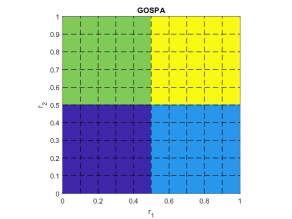
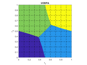
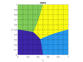
Figure 1: Decision regions for the optimal estimators based on GOSPA, UOSPA and OSPA against the existence probabilities of two Bernoulli components. Dark blue: no target is estimated. Light blue: only target 1 is estimated. Green: only target 2 is estimated. Yellow: both targets are estimated. The only metric whose optimal estimator is free from spooky effect is GOSPA ($\alpha=2$).

Example 5.

Let us consider that there are two potential targets: Bernoulli component 1 in Madrid and Bernoulli component 2 in Liverpool. These potential targets are independent of each other, but are being tracked by the same system. The probability of existences are $r_{1}=0.4$ and $r_{2}=0.4$. Therefore, the optimal OSPA estimator reports two targets, see Figure 1. We analyse the following cases

• Case 1: We receive a measurement from the potential target in Liverpool, such that $r_{2}$ increases to $r_{2}=0.9$. The measurement from the potential target in Liverpool conveys no information whatsoever on the potential target in Madrid, and $r_{1}$ is not modified. However, now, the optimal OSPA estimator only reports target 2. In other words, an increase in the probability of existence of one potential target can actually make that the other potential target is no longer being reported, even if they are independent events in far-away regions. Apart from the spooky effect, it is also interesting to observe that optimal OSPA estimation has a counter intuitive behaviour with respect to the estimation of the total number of targets in the scene. That is, before taking the measurement, the optimal OSPA estimator reports the two targets. Once we receive the measurement, the probability that there are two targets actually increases, but the optimal OSPA estimator chooses to drop one of the previously reported targets.

• Case 2: We receive a measurement from the potential target in Liverpool, such that $r_{2}$ decreases to $r_{2}=0.3$, which does not affect $r_{1}$. In this case, using an optimal OSPA estimator, both potential targets are no longer detected. As in the previous case, the optimal estimation of a potential target changes depending on a independent event in a distant region. $\boxempty$

Situations with spooky effect also arise in optimal UOSPA estimation. It is also relevant to analyse if the spooky effect at a distance is observed in other types of multi-target estimators, not based on metrics, commonly used in the literature. We consider the marginal multitarget estimator, the joint multitarget estimators (JoM) [7, 28, 29] and the estimator that first maximises the cardinality distribution and then reports the targets with largest existence probability, as in [30]. The marginal multitarget estimator and JoM are not defined when the Bernoulli densities include Dirac deltas. Nevertheless, we apply them by considering Gaussian distributions with a covariance matrix $\sigma^{2}I$, with small $\sigma^{2}$, instead of Dirac deltas in (4). We set the JoM parameter $c$ ($c$ as defined in [7, Sec. 14.5]) to $1/\mathcal{N}\left(0;0,\sigma^{2}I\right)$, which removes the dependency of the JoM on $\sigma^{2}$. The resulting decision regions of the optimal estimators are shown in Figure 2. All of them show spooky effect, as the optimal estimator for two Bernoulli components does not make decisions independently for each Bernoulli component.

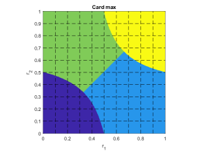
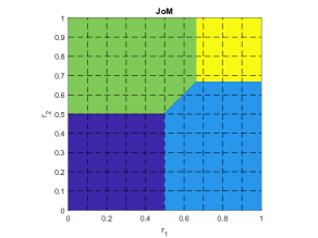
Figure 2: Decision regions for the marginal multitarget estimator, which coincide with the regions for the estimator that maximises the cardinality distribution first, (top) and the joint multitarget estimator (bottom) against the existence probabilities of two Bernoulli components. These estimators show spooky effect.

III-D Increasing number of Bernoulli components

We proceed to analyse the effect of increasing the number $N$ of Bernoulli components on the optimal estimators based on UOSPA, OSPA and GOSPA. We consider that the existence probabilities of all Bernoulli components are the same, $r_{i}=r$ for $i=1,...,N$ and that all Bernoulli components are far from each other.

In this case, the mean square UOSPA and OSPA errors can be simplified as follows

$$\mathrm{MSUOSPA} =c^{2}\left[\sum_{n=0}^{N}\rho\left(n\right)\max\left(n,\hat{n}\right)-\hat{n}r\right]$$

$$\mathrm{MSOSPA} =\begin{cases}c^{2}\left(1-\hat{n}r\sum_{n=0}^{N-1}\frac{\rho_{-1}\left(n\right)}{\max\left(n+1,\hat{n}\right)}\right)&\hat{n}>0\\ c^{2}\left(1-\rho\left(0\right)\right)&\hat{n}=0\end{cases}$$ (10)

where we have applied that $\rho_{-1}\left(\cdot\right)=\rho_{-i}\left(\cdot\right)$ for all $i$ as all the probabilities of existence are alike. Note that the above mean square errors depend on the estimated number of targets, not the individual target estimates $\hat{e}_{i}$ $i=1,...,N$, due to the fact that existence probabilities are alike.

As shown in Appendix C, the optimal estimator for MSOSPA detects $\hat{n}_{0}$ targets, with

$$\hat{n}_{0} =\begin{cases}N&\left(1-r\right)^{N}<r\\ 0&\mathrm{otherwise}.\end{cases}$$ (11)

That is, the optimal OSPA estimator either detects 0 or all the targets depending on the inequality in the previous equation, which depends on the number of Bernoulli components and the probability of existence.

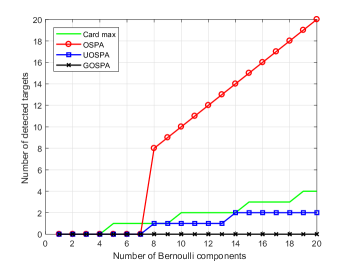
(a)

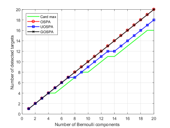
(b)

Figure 3: Optimal number of detected targets against the number of Bernoulli components at far distance for the different metrics for (a) $r=0.2$ (b) $r=0.8$. For (a) OSPA optimally detects all targets if there are more than 7 targets, otherwise it does not detect any. UOSPA optimally detects 0 targets for less than 8 Bernoulli components and then adds target detections as there are more targets. GOSPA does not detect any targets as all of them are far away with a low probability of existence. In (b), OSPA optimally detects all targets. UOSPA detects all targets if there are less than 8 Bernoulli components but then misses some of the targets for a higher number of Bernoulli components. GOSPA detects all the targets as all of them are far away with a high probability of existence. OSPA and UOSPA show spooky effect in optimal estimation as if we add independent Bernoulli components in far away regions, it affects the target reports in other regions.

We plot the number of optimally detected targets against the number of Bernoulli components for $r=0.2$ and $r=0.8$ in Figure 3. GOSPA detects a target if its probability of existence is higher than 0.5, see (9), independently of the rest of the Bernoulli components. For OSPA, we can see from (11), that, for increasing $N$, there is a point at which the optimal number of detected targets jumps directly from 0 to $N$. This means that adding an independent Bernoulli component in a far away region, even with a very small probability, can make the estimator go from no detections at all to detect all possible targets. This is a counterintuitive behaviour of a multi-target estimator in standard applications. For $r=0.8$, OSPA detects all targets for $N\geq 1$, as GOSPA.

In the case of UOSPA, for $r=0.2$, the optimal number of detected targets increases with $N$. However, UOSPA adds them one by one, which is more reasonable than the optimal OSPA estimator. For $r=0.8$, the optimal UOSPA estimator does not detect all targets as $N$ increases and it drops targets one by one. For example, for $N=8$, it does not detect one target and, for $N=14$, it does not detect two targets. Optimal UOSPA estimation has the advantage over optimal OSPA estimation that it avoids the all-or-nothing estimation effect, but it still shows spooky effect. Adding a far away Bernoulli component can either create the detection of a previously non-detected target or can remove a detection of a previously detected targets. It is also interesting to note that, as all targets have the same existence probability, an optimal UOSPA estimator can select any combination of them, with the right number of targets, to be reported. In addition, we can see that the estimator that reports the number of targets that maximises the cardinality distribution is more similar to UOSPA than to OSPA or GOSPA.

IV Conclusions

This paper has presented the spooky effect at a distance in optimal OSPA and UOSPA estimation. This effect is non desired in standard multi-target estimation, as the spooky effect in the CPHD filter [26]. The spooky effect can be avoided intrinsically by a selection of a suitable multi-target metric, the GOSPA metric, and its corresponding optimal estimator.

We think that the spooky effect in OSPA and UOSPA is a reason to support the use of GOSPA in standard multitarget tracking problems, where one aims to localise targets well and lower the number of false and missed targets. An additional benefit of GOSPA is that one can report the error decomposition along with the overall metric value to show greater insights into the performances of different algorithms, as done in [31].

We would also like to remark that there can be applications where the spooky effect, either of optimal OSPA/UOSPA estimation or the CPHD filter, can actually be beneficial. If in a certain application, it is more important to determine the overall number of objects well, compared to localising objects with sufficient accuracy and lowering missed and false objects, OSPA, UOSPA or GOSPA with general $\alpha$ may be the best choice of metric for this problem. In this case, the spooky effect should be promoted by optimal estimators. Nevertheless, in conventional multiple target tracking, the spooky effect is arguably both undesirable and counterintuitive.

Appendix A

In this appendix, we show that the optimal estimate must be a subset of $\left\{\overline{x}_{1},...,\overline{x}_{N}\right\}$ for the problem formulation in Section III. We first prove it for mean square GOSPA, with general $\alpha$. We have

$$\mathrm{MSGOSPA_{\alpha}} =\sum_{n=0}^{\infty}\frac{1}{n!}\int\left(d_{2}^{\left(c,\alpha\right)}\left(\left\{x_{1},...,x_{n}\right\},\hat{X}\right)\right)^{2}$$

$$\quad\times f\left(\left\{x_{1},...,x_{n}\right\}\right)dx_{1:n}$$

$$=\left[\prod_{i=1}^{N}\left(1-r_{i}\right)\right]\sum_{n=0}^{N}\frac{1}{n!}\sum_{1\leq i_{1}\neq...\neq i_{n}\leq N}$$

$$\,\left(d_{2}^{\left(c,\alpha\right)}\left(\hat{X},\left\{\overline{x}_{i_{1}},...,\overline{x}_{i_{n}}\right\}\right)\right)^{2}\prod_{j=1}^{n}\frac{r_{i_{j}}}{1-r_{i_{j}}}$$

$$=\left[\prod_{i=1}^{N}\left(1-r_{i}\right)\right]\sum_{n=0}^{N}\sum_{\left\{i_{1},...,i_{n}\right\}\subseteq\left\{1,...,N\right\}}$$

$$\,\left(d_{2}^{\left(c,\alpha\right)}\left(\hat{X},\left\{\overline{x}_{i_{1}},...,\overline{x}_{i_{n}}\right\}\right)\right)^{2}\prod_{j=1}^{n}\frac{r_{i_{j}}}{1-r_{i_{j}}}$$

$$=\sum_{I\subseteq\left\{1,...,N\right\}}p\left(I\right)\left(d_{2}^{\left(c,\alpha\right)}\left(\hat{X},\overline{X}\left(I\right)\right)\right)^{2}$$

where we have used the expression of the multi-Bernoulli density in [27, Eq. (4.127)] and

$$p\left(\left\{i_{1},...,i_{n}\right\}\right) =\left[\prod_{i=1}^{N}\left(1-r_{i}\right)\right]\prod_{j=1}^{n}\frac{r_{i_{j}}}{1-r_{i_{j}}},$$

$$\overline{X}\left(\left\{i_{1},...,i_{n}\right\}\right) =\left\{\overline{x}_{i_{1}},...,\overline{x}_{i_{n}}\right\}.$$

If $\hat{X}$ is a subset of $\overline{X}$, then

$$d_{2}^{\left(c,\alpha\right)}\left(\hat{X},\overline{X}\left(I\right)\right) =\frac{c^{2}}{\alpha}\left[\max\left(\left|\hat{X}\right|,\left|\overline{X}\left(I\right)\right|\right)\right.$$

$$\quad\left.-\min\left(\left|\hat{X}\right|,\left|\overline{X}\left(I\right)\right|\right)\right]$$

for all $I$. That is, for the optimal permutation, the terms that include $d^{\left(c\right)}\left(\cdot,\cdot\right)$ in the metric are always zero.

On the contrary, if $\hat{X}$ is not a subset of $\overline{X}$, then

$$d_{2}^{\left(c,\alpha\right)}\left(\hat{X},\overline{X}\left(I\right)\right) >\frac{c^{2}}{\alpha}\left[\max\left(\left|\hat{X}\right|,\left|\overline{X}\left(I\right)\right|\right)\right.$$

$$\quad\left.-\min\left(\left|\hat{X}\right|,\left|\overline{X}\left(I\right)\right|\right)\right]$$

for at least one $I\subseteq\left\{1,...,N\right\}$ because one of the terms $\sum_{i=1}^{\left|X\right|}d^{\left(c\right)}\left(x_{i},y_{\pi\left(i\right)}\right)^{2}$ in the optimal permutation must be higher than zero. Therefore, the optimal MSGOSPA estimate for any $\alpha$ must be a subset of $\overline{X}$. Similar arguments apply to OSPA.

Appendix B

In this appendix, we prove the expressions of the mean square errors for GOSPA, UOSPA and OSPA, which are given by (5), (6) and (7).

B-A GOSPA

We use variable $e_{i}=1$ to denote the case that the $i$-th Bernoulli component has an existing target and $e_{i}=0$, otherwise. Therefore, the probability of the event $e_{1:N}=\left[e_{1},...,e_{N}\right]^{T}$ is

$$p\left(e_{1:N}\right) =\prod_{i=1}^{N}\left[\left(1-r_{i}\right)\left(1-e_{i}\right)+r_{i}e_{i}\right].$$

For each pair $e_{1:N}$ and $\hat{e}_{1:N}$, it is straightforward to obtain that the square GOSPA error is

$$\mathrm{SGOSPA} =\frac{c^{2}}{2}\sum_{i=1}^{N}\left[e_{i}\left(1-\hat{e}_{i}\right)+\left(1-e_{i}\right)\hat{e}_{i}\right].$$

That is, each Bernoulli component contributes with an error $\frac{c^{2}}{2}$ if the target is not detected and exists or if the target is detected and it does not exist. Otherwise, the error for each Bernoulli component is zero.

Considering that the probability of existence of the $i$-th Bernoulli component is $r_{i}$, see (4) , the resulting $\mathrm{MSGOSPA}$ error is given in (5).

B-B UOSPA

The number of targets in the ground truth is

$$n =\sum_{i=1}^{N}e_{i}.$$

The number of targets in the estimate is $\hat{n}$, see (8). For each pair $e_{1:N}$ and $\hat{e}_{1:N}$, it is direct to obtain that the square UOSPA error is

$$\mathrm{SUOSPA} =c^{2}\left(\max\left(n,\hat{n}\right)-\sum_{i=1}^{N}\hat{e}_{i}e_{i}\right)$$ (12)

where the term $\sum_{i=1}^{N}\hat{e}_{i}e_{i}$ represents the number of properly detected targets. In this case, a properly detected target implies that the target and the estimate are in the same location. It should be noted that, each properly detected target is penalised with a zero error, and each of the rest of the targets in the largest set is penalised with an error $c^{2}$.

The mean square UOSPA error is then

$$\mathrm{MSUOSPA} =c^{2}\sum_{e_{1:N}}p\left(e_{1:n}\right)\left(\max\left(n,\hat{n}\right)-\sum_{i=1}^{N}\hat{e}_{i}e_{i}\right)$$

$$=c^{2}\left[\sum_{e_{1:N}}p\left(e_{1:n}\right)\max\left(n,\hat{n}\right)-\sum_{i=1}^{N}\hat{e}_{i}r_{i}\right]$$

$$=c^{2}\left[\sum_{n=0}^{N}\rho\left(n\right)\max\left(n,\hat{n}\right)-\sum_{i=1}^{N}\hat{e}_{i}r_{i}\right]$$

where $\rho\left(n\right)$ represents the cardinality distribution of a multi-Bernoulli density [27, page 102].

B-C OSPA

For each pair $e_{1},...,e_{N}$ and $\hat{e}_{1},...,\hat{e}_{N}$, the square OSPA error is

$$\mathrm{SOSPA} =\begin{cases}0&n=0,\,\hat{n}=0\\ c^{2}\left(1-\frac{\sum_{i=1}^{N}\hat{e}_{i}e_{i}}{\max\left(n,\hat{n}\right)}\right)&\mathrm{otherwise}\end{cases}$$

which corresponds to the square UOSPA error, see (12), normalised by $\max\left(n,\hat{n}\right)$, for $n\neq 0,\,\hat{n}\neq 0$.

The mean square OSPA error is then

$$\mathrm{MSOSPA} =\begin{cases}c^{2}\left(1-\sum_{e_{1:n}}p\left(e_{1:n}\right)\frac{\sum_{i=1}^{N}\hat{e}_{i}e_{i}}{\max\left(n,\hat{n}\right)}\right)&\hat{n}>0\\ c^{2}\left(1-\rho\left(0\right)\right)&\hat{n}=0\end{cases}$$ (13)

We proceed to simplify the term

$$\sum_{e_{1:n}}p\left(e_{1:n}\right)\frac{\sum_{i=1}^{N}\hat{e}_{i}e_{i}}{\max\left(n,\hat{n}\right)} =\sum_{i=1}^{N}\hat{e}_{i}\mathrm{E}\left[\frac{e_{i}}{\max\left(n,\hat{n}\right)}\right]$$ (14)

We first note that the total number of targets in the ground truth can be written as $n=e_{i}+n_{-i}$ where $n_{-i}$ represents the number of elements targets apart from the Bernoulli component $i$. Due to the fact that existences are independent in the Bernoulli components, we can write

$$p\left(e_{i},n_{-i}\right) =p\left(e_{i}\right)\rho_{-i}\left(n_{-i}\right)$$

where $\rho_{-i}\left(\cdot\right)$ represents the cardinality distribution of all Bernoulli components except the $i$-th one. This cardinality is known as it is the cardinality of a multi-Bernoulli distribution [27, page 102].

Then, we have

$$\mathrm{E}_{e_{i},n}\left[\frac{e_{i}}{\max\left(n,\hat{n}\right)}\right]$$

$$\quad=\mathrm{E}_{e_{i},n_{-i}}\left[\frac{e_{i}}{\max\left(n_{-i}+e_{i},\hat{n}\right)}\right]$$

$$\quad=\sum_{e_{i}=0}^{1}\sum_{n_{-i}=0}^{N-1}p\left(e_{i}\right)\rho_{-i}\left(n_{-i}\right)\frac{e_{i}}{\max\left(n_{-i}+e_{i},\hat{n}\right)}$$

$$\quad=r_{i}\sum_{n=0}^{N-1}\frac{\rho_{-i}\left(n\right)}{\max\left(n+1,\hat{n}\right)}.$$ (15)

Finally, substituting (14) and (15) into (13), we obtain (7).

B-D GOSPA with general $\alpha$

For completeness, in this appendix, we write the expression for mean square GOSPA error for general $\alpha$.

For each pair $e_{1:N}$ and $\hat{e}_{1:N}$, the square GOSPA error, general $\alpha$, is

$$\mathrm{SGOSPA}_{\alpha} =\frac{c^{2}}{\alpha}\left|n-\hat{n}\right|+c^{2}\left(\min\left(n,\hat{n}\right)-\sum_{i=1}^{N}\hat{e}_{i}e_{i}\right).$$

As before, the term $\sum_{i=1}^{N}\hat{e}_{i}e_{i}$ represents the number of properly detected targets. These targets are penalised with an error 0. Each of the rest of the targets in the smaller set is penalised with an error $c^{2}$. Finally, the difference in cardinality is penalised multiplied by a factor $\frac{c^{2}}{\alpha}$. Note that $\left|n-\hat{n}\right|=\max\left(n,\hat{n}\right)-\min\left(n,\hat{n}\right)$, so for $\alpha=1$, we recover the UOSPA error, as required.

The mean square GOSPA error is then

$$\mathrm{MSGOSPA}_{\alpha}$$

$$\,=\sum_{n=0}^{N}\left[\frac{c^{2}}{\alpha}\left|n-\hat{n}\right|+c^{2}\min\left(n,\hat{n}\right)\right]\rho\left(n\right)-c^{2}\sum_{i=1}^{N}\hat{e}_{i}r_{i}$$

Appendix C

In this appendix, we show that the optimal number of detected targets using OSPA in the scenario in Section III-D is given by (11).

First, we calculate the MSOSPA error for $\hat{n}=N$ using Eq. (10). We have

$$\mathrm{MSOSPA}\left(N\right) =c^{2}\left(1-Nr\sum_{n=0}^{N-1}\frac{\rho_{-1}\left(n\right)}{\max\left(n+1,N\right)}\right)$$

$$=c^{2}\left(1-Nr\sum_{n=0}^{N-1}\frac{\rho_{-1}\left(n\right)}{N}\right)$$

$$=c^{2}\left(1-r\sum_{n=0}^{N-1}\rho_{-1}\left(n\right)\right)$$

$$=c^{2}\left(1-r\right)$$

where in the last step we have used that the cardinality distribution of the multi-Bernoulli with $N-1$ Bernoulli components sums to one over $n=0,...,N-1$.

In addition, for $\hat{n}=0$, we can write the MSOSPA in terms of the probability of existence to yield

$$\mathrm{MSOSPA}\left(0\right) =c^{2}\left[1-\left(1-r\right)^{N}\right].$$

Therefore, it is better to detect $N$ targets instead of 0 targets if

$$\left(1-r\right)^{N} <r.$$

The next part of the proof consists of showing that

$$\mathrm{MSOSPA}\left(\hat{n}\right) >\mathrm{MSOSPA}\left(N\right)$$

for $0<\hat{n}<N$, which means that the optimal estimate has either zero or $N$ targets.

First, for $0\leq n<N$ and $0<\hat{n}<N$, it holds that

$$\hat{n} \leq\max\left(n+1,\hat{n}\right)$$

$$\frac{1}{\max\left(n+1,\hat{n}\right)} \leq\frac{1}{\hat{n}}$$

$$\frac{\rho_{-1}\left(n\right)}{\max\left(n+1,\hat{n}\right)} \leq\frac{\rho_{-1}\left(n\right)}{\hat{n}}.$$ (16)

For $n=N-1$, we have a strict inequality in (16) since $N>\hat{n}$ when $0<\hat{n}<N$. We proceed to sum over $n=0$ to $N-1$ in both sides of (16). Since we have a strict inequality in at least one term, the summation also yields a strict inequality

$$\sum_{n=0}^{N-1}\frac{\rho_{-1}\left(n\right)}{\max\left(n+1,\hat{n}\right)} <\sum_{n=0}^{N-1}\frac{\rho_{-1}\left(n\right)}{\hat{n}}$$

$$1-\hat{n}r\sum_{n=0}^{N-1}\frac{\rho_{-1}\left(n\right)}{\max\left(n+1,\hat{n}\right)} >1-\hat{n}r\sum_{n=0}^{N-1}\frac{\rho_{-1}\left(n\right)}{\hat{n}}$$

$$\mathrm{MSOSPA}\left(\hat{n}\right) >\mathrm{MSOSPA}\left(N\right)\quad 0<\hat{n}<N$$

which finishes the proof of (11).

References

- [1] S. Blackman and R. Popoli, Design and Analysis of Modern Tracking Systems. Artech House, 1999.
- [2] A. Petrovskaya and S. Thrun, “Model based vehicle detection and tracking for autonomous urban driving,” Autonomous Robots, vol. 26, no. 2, pp. 123–139, 2009.
- [3] K. Granström, L. Svensson, S. Reuter, Y. Xia, and M. Fatemi, “Likelihood-based data association for extended object tracking using sampling methods,” IEEE Transactions on Intelligent Vehicles, vol. 3, no. 1, pp. 30–45, March 2018.
- [4] S. Särkkä, Bayesian Filtering and Smoothing. Cambridge University Press, 2013.
- [5] C. P. Robert, The Bayesian Choice. Springer, 2007.
- [6] S. M. Kay, Fundamentals of Statistical Signal Processing: Estimation Theory. Prentice-Hall, 1993.
- [7] R. P. S. Mahler, Statistical Multisource-Multitarget Information Fusion. Artech House, 2007.
- [8] J. R. Hoffman and R. P. S. Mahler, “Multitarget miss distance via optimal assignment,” IEEE Transactions on Systems, Man, and Cybernetics - Part A: Systems and Humans, vol. 34, no. 3, pp. 327–336, May 2004.
- [9] E. del Barrio, J. A. Cuesta-Albertos, C. Matrán, and J. M. Rodríguez-Rodriguez, “Tests of goodness of fit based on the -Wasserstein distance,” vol. 27, no. 4, pp. 1230–1239, 1999.
- [10] C. Villani, Optimal transport: Old and New. Springer, 2009.
- [11] D. Schuhmacher, B.-T. Vo, and B.-N. Vo, “A consistent metric for performance evaluation of multi-object filters,” IEEE Transactions on Signal Processing, vol. 56, no. 8, pp. 3447–3457, Aug. 2008.
- [12] D. Schuhmacher and A. Xia, “A new metric between distributions of point processes,” vol. 40, no. 3, pp. 651–672, Sep. 2008.
- [13] M. Guerriero, L. Svensson, D. Svensson, and P. Willett, “Shooting two birds with two bullets: How to find minimum mean OSPA estimates,” in 13th Conference on Information Fusion, July 2010, pp. 1–8.
- [14] M. Baum, P. Willett, and U. D. Hanebeck, “Polynomial-time algorithms for the exact MMOSPA estimate of a multi-object probability density represented by particles,” IEEE Transactions on Signal Processing, vol. 63, no. 10, pp. 2476–2484, May 2015.
- [15] M. Baum, P. Willett, and U. Hanebeck, “Calculating some exact MMOSPA estimates for particle distributions,” in 15th International Conference on Information Fusion, 2012, pp. 847–853.
- [16] G. M. Lipsa and M. Guerriero, “A geometrical look at MOSPA estimation using transportation theory,” IEEE Signal Processing Letters, vol. 23, no. 12, pp. 1835–1838, Dec. 2016.
- [17] D. F. Crouse, P. Willett, M. Guerriero, and L. Svensson, “An approximate minimum MOSPA estimator,” in IEEE International Conference on Acoustics, Speech and Signal Processing, 2011, pp. 3644–3647.
- [18] L. Svensson, D. Svensson, M. Guerriero, and P. Willett, “Set JPDA filter for multitarget tracking,” IEEE Transactions on Signal Processing, vol. 59, no. 10, pp. 4677–4691, Oct. 2011.
- [19] J. L. Williams, “An efficient, variational approximation of the best fitting multi-Bernoulli filter,” IEEE Transactions on Signal Processing, vol. 63, no. 1, pp. 258–273, Jan. 2015.
- [20] P. Barrios, M. Adams, K. Leung, F. Inostroza, G. Naqvi, and M. E. Orchard, “Metrics for evaluating feature-based mapping performance,” IEEE Transactions on Robotics, vol. 33, no. 1, pp. 198–213, Feb. 2017.
- [21] A. S. Rahmathullah, A. F. García-Fernández, and L. Svensson, “Generalized optimal sub-pattern assignment metric,” in 20th International Conference on Information Fusion, 2017.
- [22] O. E. Drummond and B. E. Fridling, “Ambiguities in evaluating performance of multiple target tracking algorithms,” in Proceedings of the SPIE conference, 1992, pp. 326–337.
- [23] B. E. Fridling and O. E. Drummond, “Performance evaluation methods for multiple-target-tracking algorithms,” vol. 1481, 1991, pp. 371–383.
- [24] R. L. Rothrock and O. E. Drummond, “Performance metrics for multiple-sensor multiple-target tracking,” in Proc. SPIE, vol. 4048, 2000, pp. 521–531.
- [25] S. Mabbs, “A performance assessment environment for radar signal processing and tracking algorithms,” in IEEE Pacific Rim Conference on Communications, Computers and Signal Processing, vol. 1, May 1993, pp. 9–12.
- [26] D. Franken, M. Schmidt, and M. Ulmke, “"Spooky action at a distance" in the cardinalized probability hypothesis density filter,” IEEE Transactions on Aerospace and Electronic Systems, vol. 45, no. 4, pp. 1657–1664, Oct. 2009.
- [27] R. P. S. Mahler, Advances in Statistical Multisource-Multitarget Information Fusion. Artech House, 2014.
- [28] E. Baser, M. McDonald, T. Kirubarajan, and M. Efe, “A joint multitarget estimator for the joint target detection and tracking filter,” IEEE Transactions on Signal Processing, vol. 63, no. 15, pp. 3857–3871, Aug. 2015.
- [29] E. Baser, T. Kirubarajan, M. Efe, and B. Balaji, “A novel joint multitarget estimator for multi-Bernoulli models,” IEEE Transactions on Signal Processing, vol. 64, no. 19, pp. 5038–5051, Oct. 2016.
- [30] B. T. Vo and B. N. Vo, “Labeled random finite sets and multi-object conjugate priors,” IEEE Transactions on Signal Processing, vol. 61, no. 13, pp. 3460–3475, July 2013.
- [31] Y. Xia, K. Granström, L. Svensson, and A. F. García-Fernández, “Performance evaluation of multi-Bernoulli conjugate priors for multi-target filtering,” in 20th International Conference on Information Fusion, July 2017, pp. 1–8.