Opponent Aware Reinforcement Learning

Abstract

In several reinforcement learning (RL) scenarios such as security settings, there may be adversaries trying to interfere with the reward generating process for their own benefit. We introduce Threatened Markov Decision Processes (TMDPs) as a framework to support an agent against potential opponents in a RL context. We also propose a level-$k$ thinking scheme resulting in a novel learning approach to deal with TMDPs. After introducing our framework and deriving theoretical results, relevant empirical evidence is given via extensive experiments, showing the benefits of accounting for adversaries in RL while the agent learns.

L1.4

1 Introduction

Over the last decade, an increasing number of processes are being automated through the use of machine learning (ML) algorithms, being essential that these are robust and reliable, if we are to trust operations based on their output. State-of-the-art ML algorithms perform extraordinarily well on standard data, but recently they have been shown to be vulnerable to adversarial examples, data instances specifically targeted at fooling algorithms [1]. As a fundamental underlying hypothesis, these ML developments rely on the use of independent and identically distributed data for both the training and test phases, [2]. However, security aspects in ML, which form part of the field of adversarial machine learning (AML), questions the previous iid data hypothesis given the presence of adaptive adversaries ready to modify the data to obtain a benefit; consequently, the training and test distributions phases might differ. Therefore, as reviewed in [3], there is a need to model the actions of other agents.

Stemming from the pioneering work in adversarial classification (AC) in [4], the prevailing paradigm used to model the confrontation between adversaries and learning-based systems in AML has been game theory, [5], see the recent reviews [6] and [7]. This entails well-known common knowledge hypothesis, [8], which, from a fundamental point of view, are not sustainable in security applications as adversaries tend to hide and conceal information. In recent work [9], we have presented a novel framework for AC based on Adversarial Risk Analysis (ARA) [10]. ARA provides one-sided prescriptive support to an agent, maximizing her expected utility, treating the adversaries’ decisions as random variables. To forecast them, we model the adversaries’ problems. However, our uncertainty about their probabilities and utilities is propagated leading to the corresponding random optimal adversarial decisions which provide the required forecasting distributions. ARA makes operational the Bayesian approach to games, as presented in [11] or [12], facilitating a procedure to predict adversarial decisions.

The AML literature has predominantly focused on the supervised setting [6]. Our focus in this paper will be in reinforcement learning (RL). In it, an agent takes actions sequentially to maximize some cumulative reward (utility), learning from interactions with the environment. With the advent of deep learning, deep RL has faced an incredible growth [13, 14]. However, the corresponding systems may be also targets of adversarial attacks [15, 16] and robust learning methods are thus needed. A related field of interest is multi-agent RL [17], in which multiple agents try to learn to compete or cooperate. Single-agent RL methods fail in these settings, since they do not take into account the non-stationarity arising from the actions of the other agents. Thus, opponent modelling is a recent research trend in RL, see the Section 2 for a review of related literature. Here we study how the ARA framework may shed light in security RL and develop new algorithms.

One of the main contributions of the paper is that of introducing TMDPs, a framework to model adversaries that interfere with the reward generating processes in RL scenarios, focusing in supporting a specific agent in its decision making process. In addition, we provide several strategies to learn an opponent’s policy, including a level-$k$ thinking scheme and a model averaging algorithm to update the most likely adversary. To showcase its generality, we evaluate our framework in diverse scenarios such as matrix games, a security gridworld game and security resource allocation games. We also show how our framework compares favourably versus a state of the art algorithm, WoLF-PHC. Unlike previous works in multi-agent RL that focus on a particular aspect of learning, we propose a general framework and provide extensive empirical evidence of its performance.

2 Background and Related Work

Our focus will be on RL. It has been widely studied as an efficient computational approach to Markov decision processes (MDP) [18], which provide a framework for modelling a single agent making decisions while interacting within an environment. We shall refer to this agent as the decision maker (DM, she). More precisely, a MDP consists of a tuple $\left(\mathcal{S},\mathcal{A},\mathcal{T},R\right)$ where $\mathcal{S}$ is the state space with states $s$; $\mathcal{A}$ denotes the set of actions $a$ available to the DM; $\mathcal{T}:\mathcal{S}\times\mathcal{A}\rightarrow\Delta(\mathcal{S})$ is the transition distribution, where $\Delta(X)$ denotes the set of all distributions over the set $X$; and, finally, $R:\mathcal{S}\times\mathcal{A}\rightarrow\Delta(\mathbb{R})$ is the reward distribution modelling the utility that the agent perceives from state $s$ and action $a$.

In such framework, the aim of the agent is to maximize the long term discounted expected utility

$$\mathbb{E}_{\tau}\left[\sum_{t=0}^{\infty}\gamma^{t}R(a_{t},s_{t})\right]$$ (1)

where $\gamma\in(0,1)$ is the discount factor and $\tau=(s_{0},a_{0},s_{1},a_{1},\ldots)$ is a trajectory of states and actions. The DM chooses actions according to a policy $\pi:\mathcal{S}\rightarrow\Delta(\mathcal{A})$, her objective being to find a policy maximizing (1). An efficient approach to solving MDPs is Q-learning, [19]. With it, the DM maintains a function $Q:\mathcal{S}\times\mathcal{A}\rightarrow\mathbb{R}$ that estimates her expected cumulative reward, iterating according to the update rule

$$Q(s,a) :=(1-\alpha)Q(s,a)+\alpha\left(r(s,a)+\gamma\max_{a^{\prime}}Q(s^{\prime},a^{\prime})\right),$$ (2)

where $\alpha$ is a learning rate hyperparameter and $s^{\prime}$ designates the state that the agent arrives at, after having chosen action $a$ in state $s$ and received reward $r(s,a)$.

We focus on the problem of prescribing decisions to a single agent in a non stationary environment as a result of the presence of other learning agents that interfere with her reward process. In such settings, Q-learning may lead to suboptimal results, [17]. Thus, in order to support the agent, we must be able to reason about and forecast the adversaries’ behaviour. Several modelling methods have been proposed in the AI literature, as thoroughly reviewed in [3]. We are concerned with the ability of our agent to predict her adversary’s actions, so we restrict our attention to methods with this goal, covering three main general approaches: policy reconstruction, type-based reasoning and recursive learning. Methods in the first group fully reconstruct the adversary’s decision making problem, generally assuming some parametric model and fitting its parameters after observing the adversary’s behaviour. A dominant approach, known as fictitious play [20], consists of modelling the other agents by computing the frequencies of choosing various actions. As learning full adversarial models could be computationally demanding, type-based reasoning methods assume that the modelled agent belongs to one of several fully specified types, unknown a priori, and learn a distribution over the types; these methods may not reproduce the actual adversary behaviour as none of them explicitly includes the ability of other agents to reason, in turn, about its opponents’ decision making. Using explicit representations of the other agents’ beliefs about their opponents could lead to an infinite hierarchy of decision making problems, as illustrated in [21] in a much simpler class of problems. Level-$k$ thinking approaches [22] typically stop this potentially infinite regress at a level in which no more information is available, fixing the action prediction at that depth through some non-informative probability distribution.

These modelling tools have been widely used in AI research but, to the best of our knowledge, their application to Q-learning in multi-agent settings remains largely unexplored. Relevant extensions have rather focused on modelling the whole system through Markov games, instead of considering a single DM’s point of view, as we do here. The three better-known solutions include minimax-Q learning [23], where at each iteration a minimax problem needs to be solved; Nash-Q learning [24], which generalizes the previous algorithm to the non-zero sum case; or the friend-or-foe-Q learning [25], in which the DM knows in advance whether her opponent is an adversary or a collaborator. Within the bandit literature, [26] introduced a non-stationary setting in which the reward process is affected by an adversary. Our framework departs from that work since we explicitly model the opponent through several strategies described below.

The framework we propose is related to the work of [27], in which the authors propose a deep cognitive hierarchy as an approximation to a response oracle to obtain more robust policies. We instead draw on the level-$k$ thinking tradition, building opponent models that help the DM predict their behaviour. In addition, we address the issue of choosing between different cognition levels for the opponent. Our work is also related with the iPOMDP framework in [28], though the authors only address the planning problem, whereas we are interested in the learning problem as well. In addition, we introduce a more simplified algorithmic apparatus that performs well in our problems of interest. The work of [29] also addressed the setting of modelling opponents in deep RL scenarios; however, the authors rely on using a particular neural network architecture over the deep Q-network model. Instead, we tackle the problem without assuming a neural network architecture for the player policies, though our proposed scheme can be adapted to that setting. The work [30] adopted a similar experimental setting to ours, but their methods apply mostly when both players get to exactly know their opponents’ policy parameters (or a maximum-likelihood estimator of them), whereas our work builds upon estimating the opponents’ Q-function and does not require direct knowledge of the opponent’s internal parameters.

In summary, all of the proposed multi-agent Q-learning extensions are inspired by game theory with the entailed common knowledge assumptions [8], which are not realistic in the security domains of interest to us. To mitigate this assumption, we consider the problem of prescribing decisions to a single agent versus her opponents, augmenting the MDP to account for potential adversaries conveniently modifying the Q-learning rule. This will enable us to adapt some of the previously reviewed modelling techniques to the Q-learning framework, explicitly accounting for the possible lack of information about the modelled opponent. In particular, we propose here to extend Q-learning from an ARA [10] perspective, through a level-$k$ scheme [22, 31].

3 Threatened Markov Decision Processes

In similar spirit to other reformulations of MDPs, such as Constrained Markov Decision Processes [32] (in which restrictions along state trajectories are considered) or Configurable Markov Decision Processes [33] (in which the DM is able to modify the environment dynamics to accelerate learning), we propose an augmentation of a MDP to account for the presence of adversaries which perform their actions modifying state and reward dynamics, thus making the environment non-stationary. In this paper, we mainly focus on the case of a DM (agent $A$, she) facing a single opponent ($B$, he). However, we provide an extension to a setting with multiple adversaries in Section 3.4.

Definition 1.

A Threatened Markov Decision Process (TMDP) is a tuple $\left(\mathcal{S},\mathcal{A},\mathcal{B},\mathcal{T},R,p_{A}\right)$ in which $\mathcal{S}$ is the state space; $\mathcal{A}$ denotes the set of actions available to the supported agent $A$; $\mathcal{B}$ designates the set of threat actions $b$, or actions available to the adversary $B$; $\mathcal{T}:\mathcal{S}\times\mathcal{A}\times\mathcal{B}\rightarrow\Delta(\mathcal{S})$ is the transition distribution; $R:\mathcal{S}\times\mathcal{A}\times\mathcal{B}\rightarrow\Delta(\mathbb{R})$ is the reward distribution, the utility that the agent perceives from a given state $s$ and a pair $(a,b)$ of actions; and $p_{A}(b|s)$ models the DM’s beliefs about her opponent’s move, i.e., a distribution over the threats for each state $s\in\mathcal{S}$.

In our approach to TMDPs, we modify the standard Q-learning update rule (2) by averaging over the likely actions of the adversary. This way the DM may anticipate potential threats within her decision making process, and enhance the robustness of her decision making policy. Formally, we first replace (2) by

$$\begin{split}Q(s,a,b)&:=(1-\alpha)Q(s,a,b)+\\ &+\alpha\left(r(s,a,b)+\gamma\max_{a^{\prime}}\mathbb{E}_{p_{A}(b|s^{\prime})}\left[Q(s^{\prime},a^{\prime},b)\right]\right)\end{split}$$ (3)

where $s^{\prime}$ is the state reached after the DM and her adversary, respectively, adopt actions $a$ and $b$ from state $s$. We then compute its expectation over the opponent’s action argument

$$Q(s,a):=\mathbb{E}_{p_{A}(b|s)}\left[Q(s,a,b)\right].$$ (4)

We use the proposed rule to compute an $\epsilon-$greedy policy for the DM, when she is at state $s$, i.e., choose with probability $(1-\epsilon)$ the action $a^{*}=\operatorname*{arg\,max}_{a}\left[Q(s,a)\right]$ or a uniformly random action with probability $\epsilon$. A provides a proof of the convergence of the rule. Though in the experiments we focus on such $\epsilon-$greedy strategy, other sampling methods can be straightforwardly used, such as a softmax policy (see D.1 for an illustration) to learn mixed strategies.

As we do not assume common knowledge, the agent will have uncertainty regarding the adversary’s policy modelled by $p_{A}(b|s)$. However, we make the standard assumption within multi-agent RL that both agents observe their opponent’s actions (resp. rewards) after they have committed to them (resp. received them). We propose two approaches to estimating the opponent’s policy $p_{A}(b|s)$ under such assumption. We start with a case in which the adversary is considered non-strategic, that is, he acts without awareness of the DM, and then provide a level-$k$ scheme. After that, in Section 3.3 we outline a method to combine different opponent models, so we can deal with mixed behavior.

3.1 Non-strategic opponent

Consider first a stateless setting. In such case, the Q-function (3) may be written as $Q(a_{i},b_{j})$, with $a_{i}\in\mathcal{A}$ the action chosen by the DM and $b_{j}\in\mathcal{B}$ the action chosen by the adversary, assuming that $\mathcal{A}$ and $\mathcal{B}$ are discrete action spaces. Suppose the DM observes her opponent’s actions after he has implemented them. She needs to predict the action $b_{j}$ chosen by her opponent. A typical option is to model her adversary using an approach inspired by fictitious play (FP), [20]: she may compute the expected utility of action $a_{i}$ using the stateless version of (4)

$$\psi(a_{i})=\mathbb{E}_{p_{A}(b)}[Q(a,b)]=\sum_{b_{j}\in\mathcal{B}}Q(a_{i},b_{j})p_{A}(b_{j}),$$

where $p_{A}(b_{j})$ reflects $A$’s beliefs about her opponent’s actions and is computed using the empirical frequencies of the opponent past plays, with $Q(a_{i},b_{j})$ updated according to (a stateless version of) (3). Then, she chooses the action $a_{i}\in\mathcal{A}$ maximizing her expected utility $\psi(a_{i})$. We refer to this variant as FPQ-learning. Observe that while the previous approach is clearly inspired by FP, it is not the same scheme, since only one of the players (the DM) is using it to model her opponent, as opposed to the standard FP algorithm in which all players adopt it.

As described in [34], adapting ARA to a game setting requires re-framing FPQ-learning from a Bayesian perspective. Let $p_{j}=p_{B}(b_{j})$ be the probability with which the opponent chooses action $b_{j}$. We may place a Dirichlet prior $(p_{1},\ldots,p_{n})\sim\mathcal{D}(\alpha_{1},\ldots,\alpha_{n})$, where $n$ is the number of actions available to the opponent. Then, the posterior is $\mathcal{D}(\alpha_{1}+h_{1},\ldots,\alpha_{n}+h_{n})$, with $h_{i}$ being the count of action $b_{i}$, $i=1,...,n$. If we denote its posterior density function as $f(p|h)$, the DM would choose the action $a_{i}$ maximizing her expected utility, which adopts the form

$$\psi(a_{i}) =\int\left[\sum_{b_{j}\in\mathcal{B}}Q(a_{i},b_{j})p_{j}\right]f(p|h)dp$$

$$= \sum_{b_{j}\in\mathcal{B}}Q(a_{i},b_{j})\mathbb{E}_{p|h}[p_{j}]\propto\sum_{b_{j}\in\mathcal{B}}Q(a_{i},b_{j})(\alpha_{j}+h_{j}).$$

The Bayesian perspective may benefit the convergence of FPQ-learning, as we include prior information about the adversary behavior when relevant.

Generalizing the previous approach to account for states is straightforward. The Q-function has now the form $Q(s,a_{i},b_{j})$. The DM needs to assess probabilities $p_{A}(b_{j}|s)$, since it is natural to expect that her opponent behaves differently depending on the state. The supported DM will choose her action at state $s$ by maximizing

$$\psi_{s}(a_{i})=\sum_{b_{j}\in\mathcal{B}}Q(s,a_{i},b_{j})p_{A}(b_{j}|s).$$

Since $\mathcal{S}$ may be huge, even continuous, keeping track of $p_{A}(b_{j}|s)$ may incur in prohibitive memory costs. To mitigate this, we take advantage of Bayes rule as $p_{A}(b_{j}|s)\,\,\propto\,\,p(s|b_{j})p(b_{j})$. The authors of [35] proposed an efficient method for keeping track of $p(s|b_{j})$, using a hash table or approximate variants, such as the bloom filter, to maintain a count of the number of times that an agent visits each state; this is only used in the context of single-agent RL to assist for a better exploration of the environment. We propose here to keep track of $n$ bloom filters, one for each distribution $p(s|b_{j})$, for tractable computation of the opponent’s intentions in the TMDP setting. This scheme may be transparently integrated within the Bayesian paradigm, as we only need to store an additional array with the Dirichlet prior parameters $\alpha_{i}$, $i=1,\ldots,n$ for the $p(b_{j})$ part. Note that, potentially, we could store initial pseudocount as priors for each $b_{j}|s$ initializing the bloom filters with the corresponding parameter values.

As a final comment, if we assume the opponent to have memory of the previous stage actions, we could straightforwardly extend the above scheme using the concept of mixtures of Markov chains [36], thus avoiding an exponential growth in the number of required parameters and linearly controlling model complexity. For example, in case the opponent belief model is $p_{A}(b_{t}|a_{t-1},b_{t-1},s_{t})$, so that the adversary recalls the previous actions $a_{t-1}$ and $b_{t-1}$, we could factor it through a mixture

$$p_{A}(b_{t}|a_{t-1},b_{t-1},s_{t})=w_{1}p_{A}(b_{t}|a_{t-1})+w_{2}p_{A}(b_{t}|b_{t-1})+w_{3}p_{A}(b_{t}|s_{t}),$$

with $\sum_{i}w_{i}=1,w_{i}\geq 0,i=1,2,3$.

3.2 Level-$k$ thinking

The previous section described how to model a non-strategic (level-0) opponent. This can be relevant in several scenarios. However, if the opponent is strategic, he may model our supported DM as a level-0 thinker, thus making him a level-1 thinker. This chain can go up to infinity, so we will have to deal with modelling the opponent as a level-$k$ thinker, with $k$ bounded by the computational or cognitive resources of the DM.

To deal with it, we introduce a hierarchy of TMDPs in which $\emph{TMDP}_{i}^{k}$ refers to the TMDP that agent $i$ needs to optimize, while considering its rival as a level-$(k-1)$ thinker. Thus, we have the process:

• If the supported DM is a level-1 thinker, she optimizes $\emph{TMDP}_{A}^{1}$. She models $B$ as a level-0 thinker (using Section 3.1).

• If she is a level-2 thinker, the DM optimizes $\emph{TMDP}_{A}^{2}$ and models $B$ as a level-1 thinker. Consequently, this “modelled” $B$ optimizes $\emph{TMDP}_{B}^{1}$, and while doing so, he models the DM as level-0.

• In general, we have a chain of TMDPs:

  $$\emph{TMDP}_{A}^{k}\rightarrow\emph{TMDP}_{B}^{k-1}\rightarrow\emph{TMDP}_{A}^{k-2}\rightarrow\cdots$$

Exploiting the fact that TMDPs correspond to repeated interaction settings (and, by assumption, both agents observe all past decisions and rewards), each agent may estimate their counterpart’s Q-function, $\hat{Q}^{k-1}$: if the DM is optimizing $\emph{TMDP}_{A}^{k}$, she will keep her own Q-function (we refer to it as $Q_{k}$), and also an estimate $\hat{Q}_{k-1}$ of her opponent’s Q-function. This estimate may be computed by optimizing $\emph{TMDP}_{B}^{k-1}$ and so on until $k=1$. Finally, the top level DM’s policy is given by

$$\operatorname*{arg\,max}_{a_{i_{k}}}Q_{k}(s,a_{i_{k}},b_{j_{k-1}}),$$

where $b_{j_{k-1}}$ is given by

$$\operatorname*{arg\,max}_{b_{j_{k-1}}}\hat{Q}_{k-1}(s,a_{i_{k-2}},b_{j_{k-1}}),$$

and so on, until we arrive at the induction basis (level-1) in which the opponent may be modelled using the FPQ-learning approach in Section 3.1. Algorithm 1 specifies the approach for a level-2 DM.

Therefore, we need to account for her Q-function, $Q_{2}$, and that of her opponent (who will be level-1), $\hat{Q}_{1}$. Figure 1 provides a schematic view of the dependencies.

$Q_{2}$, $\hat{Q}_{1}$, $\alpha_{2},\alpha_{1}$ (DM and opponent Q-functions and learning rates, respectively).

Observe transition $(s,a,b,r_{A},r_{B},s^{\prime})$

$\hat{Q}_{1}(s,b,a):=(1-\alpha_{1})\hat{Q}_{1}(s,b,a)+\alpha_{1}(r_{B}+\gamma\max_{b^{\prime}}\mathbb{E}_{p_{B}(a^{\prime}|s^{\prime})}\left[\hat{Q}_{1}(s^{\prime},b^{\prime},a^{\prime})\right])$

Compute $B$’s estimated $\epsilon-$greedy policy $p_{A}(b|s^{\prime})$ from $\hat{Q}_{1}(s,b,a)$

$Q_{2}(s,a,b):=(1-\alpha_{2})Q_{2}(s,a,b)+\alpha_{2}(r_{A}+\gamma\max_{a^{\prime}}\mathbb{E}_{p_{A}(b^{\prime}|s^{\prime})}\left[Q_{2}(s^{\prime},a^{\prime},b^{\prime})\right])$

Algorithm 1 Level-2 thinking update rule

c.5int.73inLevel-2 (DM, denoted as A) $Q_{2}$, $p_{A}(b|s)\leftsquigarrow$ Level-1 (Adv., denoted as B) $\hat{Q}_{1}$, $p_{B}(a|s)\leftsquigarrow$ Level-0 (DM)

Figure 1: Level-$k$ thinking scheme, with $k=2$

Note that in the previous hierarchy of policies the decisions are obtained in a greedy manner, by maximizing the lower level $\hat{Q}$ estimate. We may gain insight in a Bayesian fashion by adding uncertainty to the policy at each level. For instance, at a certain level in the hierarchy, we could consider $\epsilon-$greedy policies that with probability $1-\epsilon$ choose an action according to the previous scheme and, with probability $\epsilon$, select a random action. Thus, we may impose distributions $p_{k}(\epsilon)$ at each level $k$ of the hierarchy. The mean of $p_{k}(\epsilon)$ may be an increasing function with respect to the level $k$ to account for the fact that uncertainty is higher at the upper thinking levels.

3.3 Combining Opponent Models

We have discussed a hierarchy of opponent models. In most situations the DM will not know which type of particular opponent she is facing. To deal with this, she may place a prior $p(M_{i})$ denoting her beliefs that her opponent is using a model $M_{i}$, for $i=1,\ldots,m$, the range of models that might describe her adversary’s behavior, with $\sum_{i=0}^{m}p(M_{i})=1$.

As an example, she might place a Dirichlet prior. Then, at each iteration, after having observed her opponent’s action, she may update her belief $p(M_{i})$ by increasing the count of the model $M_{i}$ which caused that action, as in the standard Dirichlet-Categorical Bayesian update rule (Algorithm 2). This is possible since the DM maintains an estimate of the opponent’s policy for each opponent model $M_{i}$, denoted $p_{M_{i}}(b|s)$. If none of the opponent models had predicted the observed action $b_{t}$, then we may not perform an update (as stated in Algorithm 2 and done in the experiments) or we could increase the count for all possible actions.

$p(M|H)\,\propto\,(n_{1},n_{2},\ldots,n_{m})$, where $H$ is the sequence $(b_{0},b_{1},\ldots,b_{t-1})$ of past opponent actions.

Observe transition $(s_{t},a_{t},b_{t},r_{A,t},r_{B,t},s_{t+1})$.

For each opponent model $M_{i}$, set $b^{i}$ to be the predicted action by model $M_{i}$.

If $b^{i}=b_{t}$ then update posterior:

$$p(M|(H||b_{t}))\,\propto\,(n_{1},\ldots,n_{i}+1,\ldots,n_{m})$$

Algorithm 2 Opponent average updating

Note that this model averaging scheme subsumes the framework of cognitive hierarchies [37], since a belief distribution is placed over the different levels of the hierarchy. However, it is more flexible since more kinds of opponents can be taken into account, for instance a minimax agent as exemplified in [34].

3.4 Facing multiple opponents

TMDPs may be extended to the case of a DM facing more than one adversary. Then, the DM would have uncertainty about all of her opponents and she would need to average her Q-function over all likely actions of all adversaries. Let $p_{A}(b^{1},\dots,b^{M}|s)$ represent the DM’s beliefs about her $M$ adversaries’ actions. The extension of the TMDP framework to multiple adversaries will require to account for all possible opponents in the DM’s Q function taking the form $Q(s,a,b^{1},\dots,b^{M})$. Finally, the DM would need to average this $Q$ over $b^{1},\dots,b^{M}$ in (3) and proceed as in (4).

In case the DM is facing non-strategic opponents, she could learn $p_{A}(b^{1},\dots,$ $b^{M}|s)$ in a Bayesian way, as explained in Section 3.1. This would entail placing a Dirichlet prior on the $n^{M}$ dimensional vector of joint actions of all adversaries. However, keeping track of those probabilities may be unfeasible as the dimension scales exponentially with the number of opponents. The case of conditionally independent adversaries turns out to be much simpler as we can use the fact that $p_{A}(b^{1},\dots,b^{M}|s)=p_{A}(b^{1}|s)\cdot\dots p_{A}(b^{M}|s)$. In this case, we could learn each $p_{A}(b^{i}|s)$ for $i=1,\dots,M$ separately, as explained in previous sections.

3.5 Computational complexity

As described before, a level-$k$ Q-learner has to estimate the Q function of a level-$(k-1)$ Q-learner, and so on. Assuming the original Q-learning update rule has time complexity $\mathcal{O}(T(|\mathcal{A}|))$, with $T$ being a factor depending on the number of actions of the DM, the update rule from Algorithm 1 has time complexity $\mathcal{O}(kT(\max\{|\mathcal{A}|,|\mathcal{B}|\}))$, i.e., linear in the level of the hierarchy.

Regarding space complexity, the overhead is also linear in the level $k$ since the DM only needs to store $k$ Q-functions, so the complexity is $\mathcal{O}(kM(|\mathcal{S}|,|\mathcal{A}|\cdot|\mathcal{B}|))$ with $M(|\mathcal{S}|,|\mathcal{A}|\cdot|\mathcal{B}|)$ accounting for the memory needed to store the Q-function in tabular form.

4 Experiments and Results

To illustrate the TMDP reasoning framework, we consider three sets of experiments: repeated matrix games, with and without memory; the adversarial security environment proposed in [38]; and a security resource allocation problem in the form of a Blotto game. The first set of experiments allows us to illustrate several relevant computational properties of our framework, whereas the second one illustrates relevant security games, our area of interest, and the last set illustrate how our framework deals with structured action spaces and multiple adversaries. All the code is released at https://github.com/vicgalle/ARAMARL, which includes full experimental setup details summarized in C.

4.1 Repeated Matrix Games

We first consider experiments with agents without memory, then agents with memory, and, finally, discuss general conclusions. As initial baseline, we focus on the stateless version of a TMDP and analyze the policies learnt by the DM, and analyze the policies learnt by the DM, who will be the row player in the corresponding matrix game, against various kinds of opponents. In all the iterated games, agent $i\in\{A,B\}$ aims at optimizing $\sum_{t=0}^{\infty}\gamma^{t}r^{i}_{t}$, and we set the discount factor $\gamma=0.96$ for illustration purposes.

4.1.1 Memoryless Repeated Matrix Games

We consider the classical Iterated Prisoner’s Dilemma (IPD), [39]. Table 1 shows its reward bimatrix. Recall that, in this game, the Nash equilibrium is (D,D).

	C	D
C	(-1, -1)	(-3, 0)
D	(0, -3)	(-2, -2)

Table 1: Payoff Matrix of Prisoners’ Dilemma

To start with, consider the opponent to be an independent-Q learner (i.e., he uses the standard Q-function from single-agent RL and (2) as learning rule). Fig. 4 depicts the utilities obtained over time by both players, in cases where we model our DM as an independent Q-learner, Fig. 2(a), or as a FPQ-learner, Fig. 2(b). An opponent-unaware DM would remain exploitable by another adversary (i.e., independent Q-learning does not converge to the Nash equilibria). Observe also that in Fig. 2(a) the variance is much bigger due to the inability of the basic Q-learning solution to deal with a non-stationary environment. In contrast, the level-1 FPQ-learner converges to the Nash equilibrium. Indeed, the DM reaches the equilibrium strategy first, becoming stationary to her opponent, and thus pulling him to play towards the equilibrium strategy. Note that the FPQ-learner is unable to learn to cooperate with her opponent, achieving lower rewards than her naive counterpart. This is due to the specification of the environment and not to a limitation of our framework since, as we shall see in Section 4.1.2, the same agent with memory of past actions is able to cooperate with its opponent, when solving the previous problem.

(a) Q-learner vs Q-learner

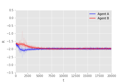
(b) FPQ-learner (blue) vs Q-learner (red)

Figure 2: Rewards obtained in IPD. We plot the trajectories of 10 simulations with shaded colors. Darker curves depict mean rewards.

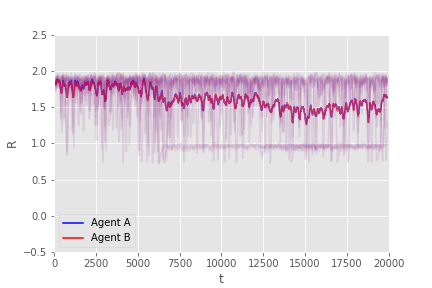
(a) Q-learner vs Q-learner

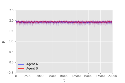
(b) FPQ-learner (blue) vs Q-learner (red)

Figure 3: Rewards in ISH game

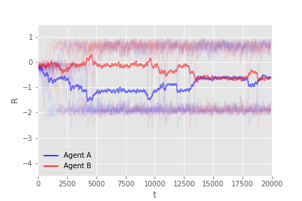
(a) Q-learner vs Q-learner

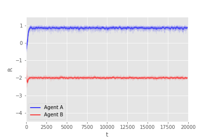
(b) FPQ-learner (blue) vs Q-learner (red)

Figure 4: Rewards in IC game

We turn to another social dilemma game, the Stag Hunt game, in which both agents must coordinate to maximize their rewards. They payoff matrix is in Table 2, with two Nash equilibria (C,C) and (D,D). We designate its iterated version ISH. We use the same experimental setting as before and report results in Figure 4.

	C	D
C	(2, 2)	(0, 1)
D	(1, 0)	(1, 1)

Table 2: Payoff Matrix of Stag Hunt

Once again, the independent learning solution cannot cope with the non-stationarity of the environment and oscillates between both equilibria without clear convergence to one of them (Fig. 3(a)). On the other hand, the FPQ-learner converges quite rapidly to the socially optimal policy (Fig. 3(b)). Then, the environment becomes essentially stationary to its opponent, who also converges to that policy.

The last social dilemma that we consider is the Chicken game, with payoff matrix in Table 3. It has two pure Nash equilibria (C, D) and (D,C). We designate its iterated variant by IC.

	C	D
C	(0, 0)	(-2, 1)
D	(1, -2)	(-4, -4)

Table 3: Payoff Matrix of Chicken

Figure 4(a) depicts again the ill convergence due to lack of opponent awareness in the independent Q-learning case; note that the instabilities continued cycling even after the limit in the displayed graphics. Alternatively, the DM with opponent modelling has an advantage and converges to her optimal Nash equilibrium (D,C) (Fig. 4(b)).

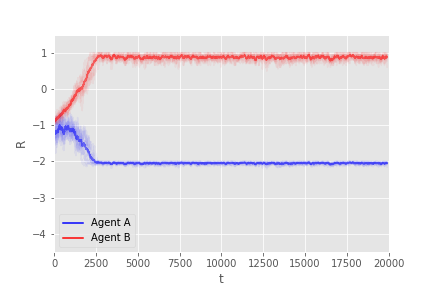
(a) FPQ-learner (blue) vs WoLF-learner (red)

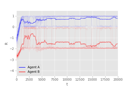
(b) L2Q-learner (blue) vs WoLF-learner (red)

Figure 5: Rewards obtained in the IC game against a WoLF-PHC adversary.

In addition, we study another kind of opponent to show how our framework can adapt to it. We consider an adversary that learns according to the WoLF-PHC algorithm [40], one of the best learning approaches in the multi-agent reinforcement learning literature. Figure 5(a) depicts a FPQ-learner (level-$1$) against this adversary, where the latter clearly exploits the former. However, if we go up in the level-$k$ hierarchy and model our DM as a level-$2$ Q-learner, she outperforms her opponent (Fig. 5(b)).

4.1.2 Repeated Matrix Games With Memory

Section 4.1.1 illustrated the ability of the modelled agents to effectively learn Nash equilibrium strategies in several iterated games. However, if we let agents have memory of previous movements, other types of equilibria may emerge, including those in which agents cooperate. We can easily augment the agents to have memory of the past $T$ joint actions taken. However, [41] proved that, in the IPD, agents with a good memory-1 strategy can effectively force the iterated game to be played as memory-1, ignoring longer play histories. Thus, we resort to memory-1 iterated games.

We restrict our attention to the IPD. We model the memory-1 IPD as a TMDP in which the state $\mathcal{S}$ adopts the form $s_{t}=(a_{t-1},b_{t-1}),\,\,t>0$ describing the previous joint action, plus the initial state $s_{0}$ in which there is no prior action. Note that now the DM’s policy is conditioned on $\mathcal{S}$, and it is fully specified by the probabilities $\pi(C|CC)$, $\pi(C|CD)$, $\pi(C|DC)$, $\pi(C|DD)$, and $\pi(C|s_{0})$.

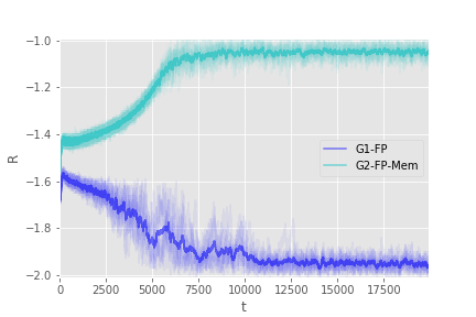
Figure 6: Rewards obtained by the DM for players: FPQ memoryless player vs TFT player (G1) and FPQ memory-1 player vs TFT player (G2).

We assume a stationary adversary playing Tit-For-Tat (TFT), i.e. replicating the opponent’s previous action [39]. TFT is a Nash equilibrium in the IPD with memory. We aim at showing that the supported DM is able to learn the equilibrium strategy.

In the experiments, the adversary will compete with either an agent playing FP (the same from the stateless environment), or with a memory-1 agent also playing FP. Figure 6 represents the utilities attained by these agents in both duels. As can be seen, a memoryless FPQ player cannot learn an optimal policy and forces the TFT agent to play defect. In contrast, augmenting this agent to have memory of the previous move allows him to learn the optimal policy (TFT), that is, he learns to cooperate, leading to a higher cumulative reward.

4.1.3 Discussion

We have shown through our examples some qualitative properties of the proposed framework. Explicitly modelling an opponent (as in the level-1 or FPQ-learner) is beneficial to maximize the rewards attained by the DM, as shown in the ISH and IC games. In both games, the DM obtains higher reward as a level-1 thinker than as a naive Q-learner against the same opponent. Also, going up in the hierarchy helps the DM to cope with more powerful opponents such as the WoLF-PHC algorithm.

In the two previous games, a level-1 DM makes both her and her opponent reach a Nash equilibrium, in contrast with the case in which the DM is a naive learner, where clear convergence is not assured. In both games there exist two pure Nash equilibria, and the higher-level DM achieved the most profitable one for her, effectively exploiting her adversary.

The case of the IPD is specially interesting. Though the level-1 DM also converges to the unique Nash equilibrium (Fig. 2(b)), it obtains less reward than its naive counterpart (Fig. 2(a)). Recall that the naive Q-learner would remain exploitable by another opponent. We argue that the FPQ-learner did not learn to cooperate, and thus achieves lower rewards, due to the specification of the game and not as a limitation of our approach. To allow for the emergence of cooperation in the IPD, agents should remember past actions taken by all players. If we specify an environment in which agents recall the last pair of actions taken, the FPQ-learner is able to cooperate (Fig. 6) with an opponent that plays a Nash optimum strategy in this modified setting, Tit-For-Tat.

4.2 AI Safety Gridworlds and Markov Security Games

A suite of RL safety benchmarks has been recently introduced in [38]. We focus on the safety friend or foe environment, in which the supported DM needs to travel a room and choose between two identical boxes, hiding positive and negative rewards, respectively. The reward assignment is controlled by an adaptive opponent. Figure 7 shows the initial state in this game. The blue cell depicts the DM’s initial state, gray cells represent the walls of the room. Cells 1 and 2 depict the adversary’s targets, who decides which one will hide the positive reward. This case may be interpreted as a spatial Stackelberg game in which the adversary is planning to attack one of two targets, and the defender will obtain a positive reward if she travels to the chosen target. Otherwise, she will miss the attacker and will incur in a loss.

As shown in [38], a deep Q-network (and, similarly, the independent tabular Q-learner as we show) fails to achieve optimal results because the reward process is controlled by the adversary. By explicitly modelling it, we actually improve Q-learning methods achieving better rewards. An alternative approach to security games in spatial domains was introduced in [42]. The authors extend the single-agent Q-learning algorithm with an adversarial policy selection inspired by the EXP3 rule from the adversarial multi-armed bandit framework in [26]. However, although robust, their approach does not explicitly model an adversary. We demonstrate that by modelling an opponent the DM can achieve higher rewards.

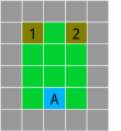
Figure 7: The friend or foe environment from the AI Safety Gridworlds benchmark. Figure taken from [38].

4.2.1 Stateless Variant

We first consider a simplified environment with a singleton state and two actions. In a spirit similar to [38], the adaptive opponent estimates the DM’s actions using an exponential smoother. Let $\bm{p}=(p_{1},p_{2})$ be the probabilities with which the DM will, respectively, choose targets 1 or 2 as estimated by the opponent. At every iteration, the opponent updates his knowledge through

$$\bm{p}:=\beta\bm{p}+(1-\beta)\bm{a},$$

where $0<\beta<1$ is a learning rate, unknown from the DM’s point of view, and $\bm{a}\in\{(1,0),(0,1)\}$ is a one-hot encoded vector indicating whether the DM chose targets 1 or 2. We consider an adversarial opponent which places the positive reward in target $t=\operatorname*{arg\,min}_{i}(\bm{p})_{i}$. Initially, the opponent has estimates $\bm{p}=(0.5,0.5)$ of the target preferred by the DM.

Since the DM has to deal with a strategic adversary, we introduce a modification to the FP-Q learning algorithm that places more attention to more recent actions. Leveraging the property that the Dirichlet distribution is a conjugate prior of the Categorical distribution, a modified update scheme is proposed in Algorithm 3.

Initialize pseudocounts $\bm{\alpha^{0}}=(\alpha^{0}_{1},\ldots,\alpha^{0}_{n})$

for $t=1,\ldots,T$ do

     $\bm{\alpha^{t}}=\lambda\bm{\alpha^{t-1}}$ $\triangleright$ Reweight with factor $0<\lambda<1$

     Observe opponent action $b^{t}_{i},i\in\{b_{1},\ldots,b_{n}\}$

     $\alpha^{t}_{i}=\alpha^{t-1}_{i}+1$ $\triangleright$ Update posterior

     $\alpha^{t}_{-i}=\alpha^{t-1}_{-i}$

end for

Algorithm 3 Dirichlet updating with forget factor

This approach essentially allows to account for the last $\frac{1}{1-\lambda}$ opponent actions, instead of weighting all observations equally. For the case of a level-2 defender, as we do not know the actual rewards of the adversary (who will be modelled as a level-1 learner), we model it as in a zero-sum scenario, i.e. $r_{B}=-r_{A}$, making this case similar to the Matching Pennies game. Other reward scalings for $r_{B}$ have been considered, though they did not qualitatively affect the results (See D.3).

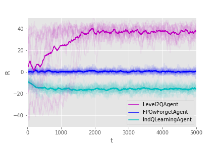
Figure 8: Rewards for the DM against the adversarial opponent

Results are displayed in Figure 8. We considered three types of defenders: an opponent unaware Q-learner, a level-1 DM with forget (Algorithm 3) and a level-2 agent. The first one is exploited by the adversary achieving suboptimal results. In contrast, the level-1 DM with forget effectively learns a stationary optimal policy (reward 0). Finally, the level-2 agent learns to exploit the adaptive adversary achieving positive rewards.

Note that the actual adversary behaves differently from how the DM models him, i.e. he is not exactly a level-1 Q-learner. Even so, modelling him as a level-1 agent gives the DM sufficient advantage.

4.2.2 Facing more powerful adversaries

Until now the DM has interacted against an exponential smoother adversary, which may be exploited if the DM is a level-2 agent. We study now the outcome of the process if we consider more powerful adversaries.

First of all, we parameterize our opponent as a level-2 Q-learner, instead of the exponential smoother. To do so, we specify the rewards he shall receive as $r_{B}=-r_{A}$, i.e., for simplicity we consider a zero-sum game, yet our framework allows for the general-sum case. Figure 9(a) depicts the rewards for both the DM (blue) and the adversary (red). We have computed the frequency for choosing each action, and both players select either action with probability $0.5\pm 0.002$ along 10 different random seeds. Both agents achieve the Nash equilibrium, consisting of choosing between both actions with equal probabilities, leading to an expected cumulative reward of 0, as shown in the graph.

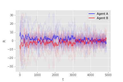
(a) L2Q-learner (blue) vs L2Q-learner (red)

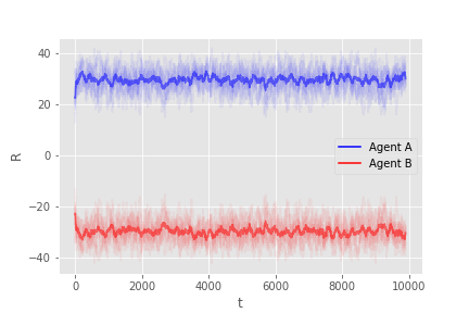
(b) L3Q-learner (blue) vs L2Q-learner (red)

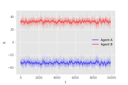
(c) L3Q-learner (blue) vs L1Q-learner (red)

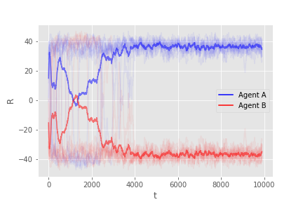
(d) L3Q-learner with opponent averaging (blue) vs L1Q-learner (red)

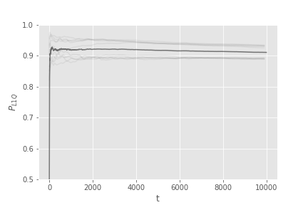
(e) Estimate of $P_{L1Q}$: DM’s belief that her opponent is a level-1 Q-learner

Figure 9: Rewards obtained against the exponential smoother adversary.

Increasing the level of our DM to make her level-3, allows her to exploit a level-2 adversary, Fig. 9(b). However, this DM fails to exploit a level-1 opponent (i.e., a FPQ-learner), Fig. 9(c). The explanation to this apparent paradox is that the DM is modelling her opponent as a more powerful agent than he actually is, so her model is inaccurate and leads to poor performance. However, the previous “failure” suggests a potential solution to the problem using type-based reasoning, Section 3.3. Figure 9(d) depicts the rewards of a DM that keeps track of both level-1 and level-2 opponent models and learns, in a Bayesian manner, which one is she actually facing. The DM keeps estimates of the probabilities $P_{L1Q}$ and $P_{L2Q}$ that her opponent is acting as if he was a level-1 or a level-2 Q-learner, respectively. Figure 9(e) depicts the evolution of $P_{L1Q}$, and we can observe that it places most of the probability in the correct opponent type.

4.2.3 Spatial Variant

We now compare the independent Q-learner and a level-$2$ Q-learner against the same adaptive opponent (exponential smoother) in the spatial gridworld domain, see Fig. 7. Target rewards are delayed until the DM arrives at one of the respective locations, obtaining $\pm 50$ depending on the target chosen by the adversary. Each step is penalized with a reward of -1 for the DM. Results are displayed in Figure 10(a). Once again, the independent Q-learner is exploited by the adversary, obtaining even more negative rewards than in Figure 8 due to the penalty taken at each step. In contrast, the level-2 agent is able to approximately estimate the adversarial behavior, modelling him as a level-1 agent, thus being able to obtain positive rewards. Figure 10(b) depicts rewards of a DM that keeps opponent models for both level-1 and level-2 Q-learners. Note that although the adversary is of neither class, the DM achieves positive rewards, suggesting that the framework is capable of generalizing between different model opponents.

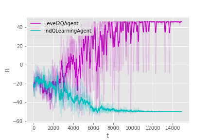
(a) Rewards for various DM models

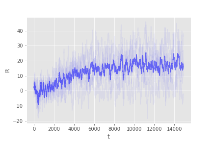
(b) Rewards for a DM with opponent models for a L1 Q-learner and a L2 Q-learner (red)

Figure 10: Rewards against the adversarial (exponential smoother) opponent in the spatial environment.

4.3 TMDPs for Security Resource Allocation

We illustrate the multiple opponent concepts of Section 3.4 introducing a novel suite of resource allocation experiments which are relevant in security settings. We propose a modified version of Blotto games [43]: the DM needs to distribute limited resources over several positions which are susceptible of being attacked. In the same way, each of the attackers has to choose different positions where they can deploy their attacks. Associated with each of the attacked positions there is a positive (negative) reward of value 1 (-1). If the DM deploys more resources than the attacks deployed in a particular position, she wins the positive reward; the negative reward will be equally divided between the attackers that chose to attack that position. If the DM deploys less resources, she will receive the negative reward and the positive one will be equally divided between the corresponding attackers. In case of a draw in a given position, no player receives any reward.

We compare the performance of a FPQ-learning agent and a standard Q-learning agent, facing two independent opponents that are both using exponential smoothing to estimate the probability of the DM placing a resource at each position, and implementing the attack where this probability is the smallest (obviously both opponents perform exactly the same attacks). To that end, we consider the problem of defending three different positions. The DM needs to allocate two resources among the different positions.

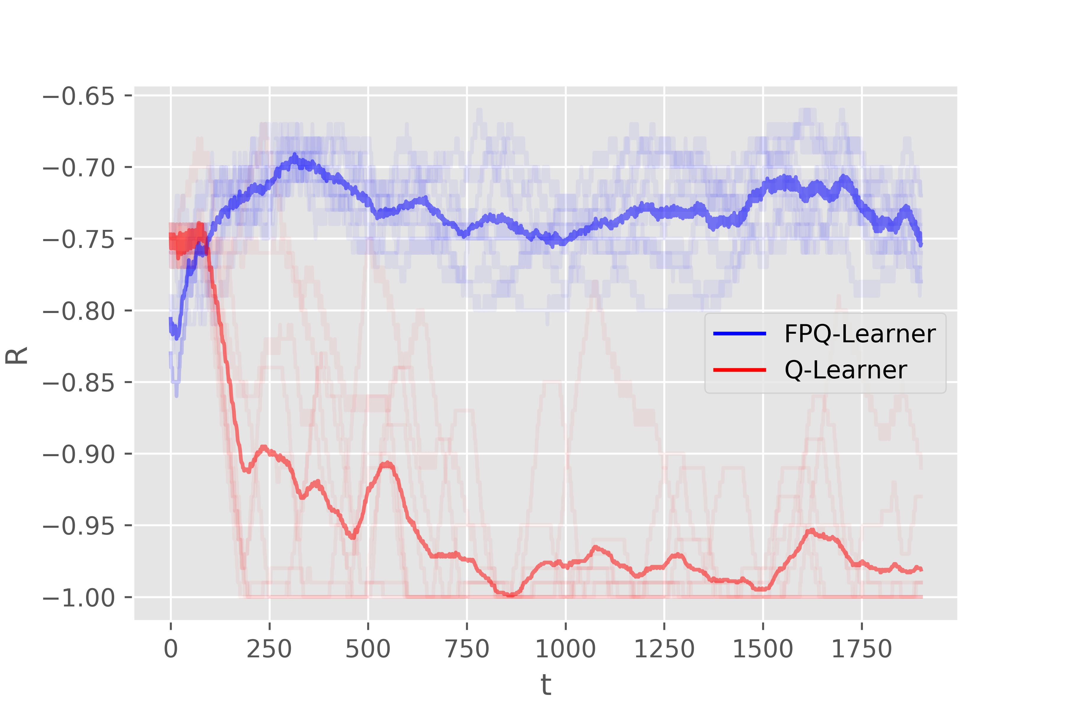
Figure 11: Rewards for the DM against the adversarial opponent

As can be seen in Fig. 11, the FPQ-learning is able to learn the opponents strategy and thus is less exploitable than the standard Q-learning agent. This experiment showcases the suitability of the framework to deal with multiple adversaries.

5 Conclusions and Further Work

We have introduced TMDPs, a novel reformulation of MDPs. This is an original framework to support decision makers who confront opponents that interfere with the reward generating process in RL settings. TMDPs aim at providing one-sided prescriptive support to a RL agent, maximizing her expected utility, taking into account potential negative actions adopted by an adversary. Some theoretical results are provided. In particular, we prove that our proposed learning rule is a contraction mapping so that we may use RL convergence results. In addition, the proposed framework is suitable for using existing opponent modelling methods within Q-learning. Indeed, we propose a scheme to model adversarial behavior based on level-$k$ reasoning about opponents. We extend this approach using type-based reasoning to account for uncertainty about the opponent’s level.

Empirical evidence is provided via extensive experiments, with encouraging results, namely the ability of the TMDP formalism to achieve Nash equilibria in repeated matrix games with an efficient computational scheme, as well as promote cooperation. In security settings, we provide empirical evidence that by explicitly modelling a finite set of adversaries via the opponent averaging scheme, the supported DM can take advantage of her actual opponent, even when he is not explicitly modelled by a component from the finite mixture. This highlights the ability of the proposed framework to generalize between different kinds of opponents. As a general lesson, we find that a level-2 Q-learner effectively deals with a wide class of adversaries. However, maintaining a mixture of different adversaries is necessary if we consider a level-3 DM. As a rule of thumb, the supported DM may start at a low level in the hierarchy, and switch to a level-up temporarily, to check if the obtained rewards are higher. Otherwise, she may continue on the initial, lower level.

Several lines of work are possible for further research. First of all, in the experiments, we have just considered up to level-3 DMs, though the extension to higher order adversaries is straightforward. In recent years Q-learning has benefited from advances from the deep learning community, with breakthroughs such as the deep Q-network (DQN) which achieved super-human performance in control tasks such as the Atari games [13], or as inner blocks inside systems that play Go [14]. Integrating these advances into the TMDP setting is another possible research path. In particular, the proposed Algorithm 1 can be generalized to account for the use of deep Q-networks instead of tabular Q-learning as presented here. We show details of the modified algorithm in B. Indeed, the proposed scheme is model agnostic, i.e., it does not matter if we represent the Q-function using a look-up table or a deep neural network, so we expect it to be usable in both shallow and deep multi-agent RL settings. In addition, there are several other ways to model the adversary’s behavior that do not require to learn opponent Q-values, for instance by using policy gradient methods [44]. Finally, it might be interesting to explore similar expansions to semi-MDPs, in order to perform hierarchical RL or to allow for time-dependent rewards and transitions between states.

Acknowledgements. VG acknowledges support from grant FPU16-05034, RN acknowledges support from the Spanish Ministry for his grant FPU15-03636. DRI is grateful to the MINCIU MTM2017-86875-C3-1-R project and the AXA-ICMAT Chair in Adversarial Risk Analysis. All authors acknowledge support from the Severo Ochoa Excellence Programme SEV-2015-0554. We are also very grateful to the numerous pointers and suggestions by the referees. This version of the manuscript was prepared while the authors were visiting SAMSI within the Games and Decisions in Risk and Reliability program.

Appendix A Sketch of proof of convergence of the update rule for TDMPs (Eqs. (3) and (4))

Consider an augmented state space so that transitions are of the form

$$(s,b)\xrightarrow[]{a}(s^{\prime},b^{\prime})\xrightarrow[]{a^{\prime}}\ldots.$$

Under this setting, the DM does not observe the full state since she does not know the action $b$ taken by her adversary. However, if she knows his policy $p(b|s)$, or has a good estimate of it, she can take advantage of this information.

Assume for now that we know the current opponent’s action $b$. The $Q$-function would satisfy the following recursive update [19],

$$Q^{\pi}(s,a,b) =\sum_{s^{\prime}}\sum_{b^{\prime}}p(s^{\prime},b^{\prime}|s,a,b)\left[R_{ss^{\prime}}^{ab}+\mathbb{E}_{\pi(a^{\prime}|s^{\prime},b^{\prime})}\left[Q^{\pi}(s^{\prime},a^{\prime},b^{\prime})\right]\right],$$

where we have taken into account explicitly the structure of the state space and used $R_{ss^{\prime}}^{ab}=\mathbb{E}\left[r_{t+1}|s_{t+1}=s^{\prime},s_{t}=s,a_{t}=a,b_{t}=b\right]$. As the next opponent action is conditionally independent of his previous action, the previous DM action and the previous state, given the current state, we may write $p(s^{\prime},b^{\prime}|s,a,b)=p(b^{\prime}|s^{\prime})p(s^{\prime}|s,a,b)$. Thus

$$Q^{\pi}(s,a,b) =\sum_{s^{\prime}}p(s^{\prime}|s,a,b)\left[R_{ss^{\prime}}^{ab}+\mathbb{E}_{p(b^{\prime}|s^{\prime})}\mathbb{E}_{\pi(a^{\prime}|s^{\prime},b^{\prime})}\left[Q^{\pi}(s^{\prime},a^{\prime},b^{\prime})\right]\right]$$

as $R_{ss^{\prime}}^{ab}$ does not depend on the next opponent action $b^{\prime}$. Finally, the optimal Q-function verifies

$$Q^{*}(s,a,b)=\sum_{s^{\prime}}p(s^{\prime}|s,a,b)\left[R_{ss^{\prime}}^{ab}+\gamma\max_{a^{\prime}}\mathbb{E}_{p(b^{\prime}|s^{\prime})}\left[Q^{*}(s^{\prime},a^{\prime},b^{\prime})\right]\right],$$

since in this case $\pi(a|s)=\operatorname*{arg\,max}_{a}Q^{*}(s,a)$. Observe now that:

Lemma 1.

Given $q:\mathcal{S}\times\mathcal{B}\times\mathcal{A}\rightarrow\mathbb{R}$, the operator $\mathcal{H}$

$$(\mathcal{H}q)(s,b,a)=\sum_{s^{\prime}}p(s^{\prime}|s,b,a)\big{[}r(s,b,a)+\gamma\max_{a^{\prime}}\mathbb{E}_{p(b^{\prime}|s^{\prime})}q(s^{\prime},b^{\prime},a^{\prime})\big{]}.$$

is a contraction mapping under the supremum norm.

Proof.

We prove that $\|\mathcal{H}q_{1}-\mathcal{H}q_{2}\|_{\infty}\leq\gamma\|q_{1}-q_{2}\|_{\infty}$.

$$\|\mathcal{H}q_{1}-\mathcal{H}q_{2}\|_{\infty}=$$

$$=\max_{s,b,a}\lvert\sum_{s^{\prime}}p(s^{\prime}|s,b,a)\big{[}r(s,b,a)+\gamma\max_{a^{\prime}}\mathbb{E}_{p(b^{\prime}|s^{\prime})}q_{1}(s^{\prime},b^{\prime},a^{\prime})$$

$$-r(s,b,a)-\gamma\max_{a^{\prime}}\mathbb{E}_{p(b^{\prime}|s^{\prime})}q_{2}(s^{\prime},b^{\prime},a^{\prime})\big{]}\rvert=$$

$$=\gamma\max_{s,b,a}\lvert\sum_{s^{\prime}}p(s^{\prime}|s,b,a)\big{[}\max_{a^{\prime}}\mathbb{E}_{p(b^{\prime}|s^{\prime})}q_{1}(s^{\prime},b^{\prime},a^{\prime})$$

$$-\max_{a^{\prime}}\mathbb{E}_{p(b^{\prime}|s^{\prime})}q_{2}(s^{\prime},b^{\prime},a^{\prime})\big{]}\rvert\leq$$

$$=\gamma\max_{s,b,a}\sum_{s^{\prime}}p(s^{\prime}|s,b,a)\lvert\max_{a^{\prime}}\mathbb{E}_{p(b^{\prime}|s^{\prime})}q_{1}(s^{\prime},b^{\prime},a^{\prime})$$

$$-\max_{a^{\prime}}\mathbb{E}_{p(b^{\prime}|s^{\prime})}q_{2}(s^{\prime},b^{\prime},a^{\prime})\rvert\leq$$

$$=\gamma\max_{s,b,a}\sum_{s^{\prime}}p(s^{\prime}|s,b,a)\max_{a^{\prime},z}\lvert\mathbb{E}_{p(b^{\prime}|z)}q_{1}(z,b^{\prime},a^{\prime})$$

$$-\mathbb{E}_{p(b^{\prime}|z)}q_{2}(z,b^{\prime},a^{\prime})\rvert\leq$$

$$=\gamma\max_{s,b,a}\sum_{s^{\prime}}p(s^{\prime}|s,b,a)\max_{a^{\prime},z,b^{\prime}}\lvert q_{1}(z,b^{\prime},a^{\prime})-q_{2}(z,b^{\prime},a^{\prime})\rvert=$$

$$=\gamma\max_{s,b,a}\sum_{s^{\prime}}p(s^{\prime}|s,b,a)\|q_{1}-q_{2}\|_{\infty}=$$

$$=\gamma\|q_{1}-q_{2}\|_{\infty}.$$

∎

Then, using the proposed learning rule (3), we would converge to the optimal $Q$ for each of the opponent actions. The proof follows directly from the standard Q-learning convergence proof, see e.g. [45], and making use of the previous Lemma.

However, at the time of making the decision, we do not know what action he would take. Thus, we suggest to average over the possible opponent actions, weighting each by $p(b|s)$, as in (4).

Appendix B Generalization to deep-Q learning

The tabular version of Q-learning introduced in Algorithm 1 does not scale well when the state or action spaces dramatically grow in size. To this end, we expand the framework to the case when the Q-functions are instead represented using a function approximator, typically a deep Q-network [13]. Algorithm 4 shows the details. The parameters $\phi_{A}$ and $\phi_{B}$ refer to the weights of the corresponding networks approximating the Q-values.

$Q_{\phi_{A}}$, $Q_{\phi_{B}}$, $\alpha_{2},\alpha_{1}$ (DM and opponent Q-functions and learning rates, respectively).

Observe transition $(s,a,b,r_{A},r_{B},s^{\prime})$.

$\phi_{B}:=\phi_{B}-\alpha_{1}\frac{\partial Q_{\phi_{B}}}{\partial\phi_{B}}(s,b,a)\left[Q_{\phi_{B}}(s,b,a)-(r_{B}+\gamma\max_{b^{\prime}}\mathbb{E}_{p_{B}(a^{\prime}|s^{\prime})}Q_{\phi_{B}}(s^{\prime},b^{\prime},a^{\prime}))\right]$

Compute B’s estimated $\epsilon-$greedy policy $p_{A}(b|s^{\prime})$ from $Q_{\phi_{B}}(s,b,a)$.

$\phi_{A}:=\phi_{A}-\alpha_{2}\frac{\partial Q_{\phi_{A}}}{\partial\phi_{A}}(s,a,b)\left[Q_{\phi_{A}}(s,a,b)-(r_{A}+\gamma\max_{a^{\prime}}\mathbb{E}_{p_{A}(b^{\prime}|s^{\prime})}Q_{\phi_{A}}(s^{\prime},a^{\prime},b^{\prime}))\right]$

Algorithm 4 Level-2 thinking update rule using neural approximators.

Appendix C Experiment Details

We describe hyperparameters and other technical details used in the experiments.

Repeated matrix games

Memoryless Repeated Matrix Games

In all three games (IPD, ISH, IC) we considered a discount factor $\gamma=0.96$, a total of max steps $T=20000$, initial $\epsilon=0.1$ and learning rate $\alpha=0.3$. The FP-Q learner started the learning process with a Beta prior $\mathcal{B}(1,1)$.

Repeated Matrix Games With Memory

In the IPD game we considered a discount factor $\gamma=0.96$, a total of max steps $T=20000$, initial $\epsilon=0.1$ and learning rate $\alpha=0.05$. The FP-Q learner started the learning process with a Beta prior $\mathcal{B}(1,1)$.

AI Safety Gridworlds

Stateless Variant

Rewards for the DM are $50,-50$ depending on her action and the target chosen by the adversary. We considered a discount factor $\gamma=0.8$ and a total of $5000$ episodes. For all three agents, the initial exploration parameter was set to $\epsilon=0.1$ and learning rate $\alpha=0.1$. The FP-Q learner with forget factor used $\lambda=0.8$.

Spatial Variant

Episodes end at a maximum of 50 steps or agent arriving first at target 1 or 2. Rewards for the DM are $-1$ for performing any action (i.e., a step in some of the four possible directions) or $50,-50$ depending on the target chosen by the adversary. We considered a discount factor $\gamma=0.8$ and a total of $15000$ episodes. For the level-2 agent, initial $\epsilon_{A}=\epsilon_{B}=0.99$ with decaying rules $\epsilon_{A}:=0.995\epsilon_{A}$ and $\epsilon_{B}:=0.9\epsilon_{B}$ every $10$ episodes and learning rates $\alpha_{2}=\alpha_{1}=0.05$. For the independent Q-learner we set initial exploration rate $\epsilon=0.99$ with decaying rule $\epsilon:=0.995\epsilon$ every $10$ episodes and learning rate $\alpha=0.05$.

TMDPs for Security Resource Allocation

For both the Q-learning and the FPQ-learning agents we considered a discount factor $\gamma=0.96$, $\epsilon=0.1$ and a learning rate of $0.1$.

Appendix D Additional Results

D.1 Alternative policies

Although we have focused in pure strategies, dealing with mixed ones is straightforward as it just entails changing the $\epsilon-$greedy policy with the softmax policy.

In this Appendix we perform an experiment in which we replace the $\epsilon-$greedy policy of the DM with a softmax policy in the spatial gridworld environment from Section 4.2. Actions at state $s$ are taken with probability proportional to $Q(s,a)$. See Figure 12 for several simulation runs of a level-2 Q-learner versus the adversary, showing that indeed changing the policy sampling scheme does not make the DM worse than its $\epsilon-$greedy alternative.

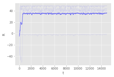
Figure 12: Rewards for the DM against the adversarial opponent, using a softmax policy.

D.2 Robustness to hyperparameters

We perform several experiments in which we try different values of the hyperparameters, just to highlight the robustness of the framework. Table 4 displays mean rewards (and standard deviations) for five different random seeds, over different hyperparameters of Algorithm 1. Except in the case where the initial exploration rate $\epsilon_{0}$ is set to a high value (0.5, which makes the DM to achieve a positive mean reward), the other settings showcase that the framework (for the level-2 case) is robust to different learning rates.

Table 4: Results on hyperparameter robustness of Algorithm 1 on the spatial gridworld.

$\alpha_{2}$	$\alpha_{1}$	$\epsilon_{0}$	Mean Reward
0.01	0.005	0.5	$15.46\pm 47.21$
0.01	0.005	0.1	$40.77\pm 27.48$
0.01	0.005	0.01	$46.32\pm 16.15$
0.01	0.02	0.5	$15.58\pm 47.17$
0.01	0.02	0.1	$43.05\pm 23.65$
0.01	0.02	0.01	$47.81\pm 10.83$
0.1	0.05	0.5	$15.30\pm 47.27$
0.1	0.05	0.1	$42.82\pm 24.08$
0.1	0.05	0.01	$48.34\pm 8.10$
0.1	0.2	0.5	$15.97\pm 47.03$
0.1	0.2	0.1	$43.05\pm 23.66$
0.1	0.2	0.01	$48.51\pm 6.96$
0.5	0.25	0.5	$15.95\pm 47.04$
0.5	0.25	0.1	$43.06\pm 23.64$
0.5	0.25	0.01	$48.41\pm 7.68$
0.5	1.0	0.5	$15.19\pm 47.31$
0.5	1.0	0.1	$42.98\pm 23.71$
0.5	1.0	0.01	$48.53\pm 6.82$

D.3 Robustness to reward scaling

For the experiments from Section 4.2.1 we tried other models for the opponent’s rewards $r_{B}$. Instead of assuming a minimax setting ($r_{B}=-r_{A}$), where $r_{B}\in\{-50,50\}$, we tried also two different scalings $r_{B}\in\{-1,1\}$ and $r_{B}\in\{0,1\}$. These alternatives are displayed in Figure 13. We found that they did not qualitatively affect the results.

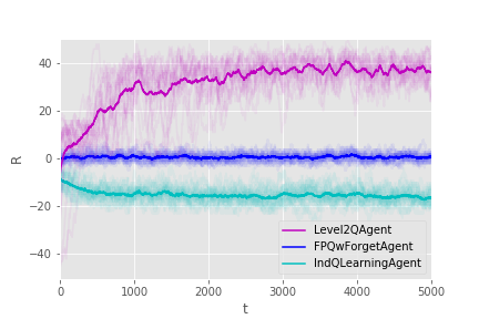
(a) Rewards $+1$ and $0$ for the adversary

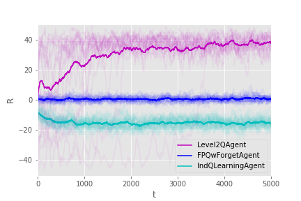
(b) Rewards $+1$ and $-1$ for the adversary

Figure 13: Rewards against the same adversary (exponential smoother) using different reward scalings.

References

References

- Goodfellow et al. [2014] I. J. Goodfellow, J. Shlens, C. Szegedy, Explaining and harnessing adversarial examples, arXiv preprint arXiv:1412.6572 (2014).
- Carbonell [1989] J. G. Carbonell, Introduction:paradigms for machine learning, Artificial Intelligence 40 (1989) 1 – 9.
- Albrecht and Stone [2018] S. V. Albrecht, P. Stone, Autonomous agents modelling other agents: A comprehensive survey and open problems, Artif. Intell. 258 (2018) 66–95.
- Dalvi et al. [2004] N. Dalvi, P. Domingos, S. Sanghai, D. Verma, et al., Adversarial classification, in: Proceedings of the tenth ACM SIGKDD international conference on Knowledge discovery and data mining, ACM, 2004, pp. 99–108.
- Menache and Ozdaglar [2011] I. Menache, A. Ozdaglar, Network games: Theory, models, and dynamics, Synthesis Lectures on Communication Networks 4 (2011) 1–159.
- Biggio and Roli [2018] B. Biggio, F. Roli, Wild patterns: Ten years after the rise of adversarial machine learning, Pattern Recognition 84 (2018) 317 – 331.
- Zhou et al. [2018] Y. Zhou, M. Kantarcioglu, B. Xi, A survey of game theoretic approach for adversarial machine learning, Wiley Interdisciplinary Reviews: Data Mining and Knowledge Discovery (2018) e1259.
- Hargreaves-Heap and Varoufakis [2004] S. Hargreaves-Heap, Y. Varoufakis, Game Theory: A Critical Introduction, Taylor & Francis, 2004.
- Naveiro et al. [2019] R. Naveiro, A. Redondo, D. R. Insua, F. Ruggeri, Adversarial classification: An adversarial risk analysis approach, International Journal of Approximate Reasoning (2019).
- R. Insua et al. [2009] D. R. Insua, J. Rios, D. Banks, Adversarial risk analysis, Journal of the American Statistical Association 104 (2009) 841–854.
- Kadane and Larkey [1982] J. B. Kadane, P. D. Larkey, Subjective probability and the theory of games, Management Science 28 (1982) 113–120.
- Raiffa [1982] H. Raiffa, The Art and Science of Negotiation, Belknap Press of Harvard University Press, 1982.
- Mnih et al. [2015] V. Mnih, K. Kavukcuoglu, D. Silver, A. A. Rusu, J. Veness, M. G. Bellemare, A. Graves, M. Riedmiller, A. K. Fidjeland, G. Ostrovski, et al., Human-level control through deep reinforcement learning, Nature 518 (2015) 529.
- Silver et al. [2017] D. Silver, J. Schrittwieser, K. Simonyan, I. Antonoglou, A. Huang, A. Guez, T. Hubert, L. Baker, M. Lai, A. Bolton, et al., Mastering the game of go without human knowledge, Nature 550 (2017) 354.
- Huang et al. [2017] S. Huang, N. Papernot, I. Goodfellow, Y. Duan, P. Abbeel, Adversarial attacks on neural network policies, arXiv preprint arXiv:1702.02284 (2017).
- Lin et al. [2017] Y.-C. Lin, Z.-W. Hong, Y.-H. Liao, M.-L. Shih, M.-Y. Liu, M. Sun, Tactics of adversarial attack on deep reinforcement learning agents, arXiv preprint arXiv:1703.06748 (2017).
- Buşoniu et al. [2010] L. Buşoniu, R. Babuška, B. De Schutter, Multi-agent reinforcement learning: An overview, in: Innovations in multi-agent systems and applications-1, Springer, 2010, pp. 183–221.
- Howard [1960] R. A. Howard, Dynamic Programming and Markov Processes, MIT Press, Cambridge, MA, 1960.
- Sutton and Barto [2018] R. S. Sutton, A. G. Barto, Reinforcement learning: An introduction, MIT press, 2018.
- Brown [1951] G. W. Brown, Iterative solution of games by fictitious play, Activity Analysis of Production and Allocation (1951) 374–376.
- Rios and Insua [2012] J. Rios, D. R. Insua, Adversarial risk analysis for counterterrorism modeling, Risk Analysis: An International Journal 32 (2012) 894–915.
- Stahl and Wilson [1994] D. O. Stahl, P. W. Wilson, Experimental evidence on players’ models of other players, Journal of economic behavior & organization 25 (1994) 309–327.
- Littman [1994] M. L. Littman, Markov games as a framework for multi-agent reinforcement learning, in: Machine Learning Proceedings 1994, Elsevier, 1994, pp. 157–163.
- Hu and Wellman [2003] J. Hu, M. P. Wellman, Nash Q-learning for general-sum stochastic games, Journal of machine learning research 4 (2003) 1039–1069.
- Littman [2001] M. L. Littman, Friend-or-Foe Q-learning in General-Sum Games, in: Proceedings of the Eighteenth International Conference on Machine Learning, Morgan Kaufmann Publishers Inc., 2001, pp. 322–328.
- Auer et al. [1995] P. Auer, N. Cesa-Bianchi, Y. Freund, R. E. Schapire, Gambling in a rigged casino: The adversarial multi-armed bandit problem, in: Foundations of Computer Science, 1995. Proceedings., 36th Annual Symposium on, IEEE, 1995, pp. 322–331.
- Lanctot et al. [2017] M. Lanctot, V. Zambaldi, A. Gruslys, A. Lazaridou, K. Tuyls, J. Pérolat, D. Silver, T. Graepel, A unified game-theoretic approach to multiagent reinforcement learning, in: Advances in Neural Information Processing Systems, 2017, pp. 4190–4203.
- Gmytrasiewicz and Doshi [2005] P. J. Gmytrasiewicz, P. Doshi, A framework for sequential planning in multi-agent settings, Journal of Artificial Intelligence Research 24 (2005) 49–79.
- He et al. [2016] H. He, J. Boyd-Graber, K. Kwok, H. Daumé III, Opponent modeling in deep reinforcement learning, in: International Conference on Machine Learning, 2016, pp. 1804–1813.
- Foerster et al. [2018] J. Foerster, R. Y. Chen, M. Al-Shedivat, S. Whiteson, P. Abbeel, I. Mordatch, Learning with opponent-learning awareness, in: Proceedings of the 17th International Conference on Autonomous Agents and MultiAgent Systems, International Foundation for Autonomous Agents and Multiagent Systems, 2018, pp. 122–130.
- Stahl and Wilson [1995] D. O. Stahl, P. W. Wilson, On players’ models of other players: Theory and experimental evidence, Games and Economic Behavior 10 (1995) 218–254.
- Altman [1999] E. Altman, Constrained Markov Decision Processes, volume 7, CRC Press, 1999.
- Metelli et al. [2018] A. M. Metelli, M. Mutti, M. Restelli, Configurable Markov Decision Processes, International Conference on Machine Learning (2018). arXiv:1806.05415.
- R. Insua et al. [2016] D. R. Insua, D. Banks, J. Rios, Modeling opponents in adversarial risk analysis, Risk Analysis 36 (2016) 742–755.
- Tang et al. [2017] H. Tang, R. Houthooft, D. Foote, A. Stooke, O. X. Chen, Y. Duan, J. Schulman, F. DeTurck, P. Abbeel, # exploration: A study of count-based exploration for deep reinforcement learning, in: Advances in Neural Information Processing Systems, 2017, pp. 2750–2759.
- Raftery [1985] A. E. Raftery, A model for high-order markov chains, Journal of the Royal Statistical Society. Series B (Methodological) (1985) 528–539.
- Camerer et al. [2004] C. F. Camerer, T.-H. Ho, J.-K. Chong, A cognitive hierarchy model of games, The Quarterly Journal of Economics 119 (2004) 861–898.
- Leike et al. [2017] J. Leike, M. Martic, V. Krakovna, P. A. Ortega, T. Everitt, A. Lefrancq, L. Orseau, S. Legg, AI safety gridworlds, arXiv preprint arXiv:1711.09883 (2017).
- Axelrod [1984] R. Axelrod, The Evolution of Cooperation, Basic, New York, 1984.
- Bowling and Veloso [2001] M. Bowling, M. Veloso, Rational and convergent learning in stochastic games, in: Proceedings of the 17th international joint conference on Artificial intelligence-Volume 2, Morgan Kaufmann Publishers Inc., 2001, pp. 1021–1026.
- Press and Dyson [2012] W. H. Press, F. J. Dyson, Iterated prisoner’s dilemma contains strategies that dominate any evolutionary opponent, Proceedings of the National Academy of Sciences 109 (2012) 10409–10413.
- Klima et al. [2016] R. Klima, K. Tuyls, F. Oliehoek, Markov security games: Learning in spatial security problems, NIPS Workshop on Learning, Inference and Control of Multi-Agent Systems (2016).
- Hart [2008] S. Hart, Discrete Colonel Blotto and General Blotto Games, International Journal of Game Theory 36 (2008) 441–460.
- Baxter and Bartlett [2000] J. Baxter, P. L. Bartlett, Direct gradient-based reinforcement learning, in: 2000 IEEE International Symposium on Circuits and Systems. Emerging Technologies for the 21st Century. Proceedings (IEEE Cat No. 00CH36353), volume 3, IEEE, 2000, pp. 271–274.
- Melo [2001] F. S. Melo, Convergence of q-learning: A simple proof, Tech. Rep. (2001).