Reduction of the Uncertainty in the Atmospheric Neutrino Flux Prediction Below 1 GeV Using Accurately Measured Atmospheric Muon Flux

Abstract

We examine the uncertainty of the calculation of the atmospheric neutrino flux due to the uncertainty in the hadronic interaction, and present a way to reduce it using accurately measured atmospheric muon flux. Considering the difference in the hadronic interaction model and the real one as a variation of hadronic interaction, we find a quantitative estimation method for the error of the atmospheric neutrino flux calculation from the reconstruction residual of the atmospheric muon flux observed in a precision experiment. However, the relation of the calculation error of the neutrino flux and the reconstruction residual of the muon flux is largely dependent on the atmospheric muon observation site, especially for the low energy neutrinos. We study the relation at several observation sites, near Kamioka at sea level, same but 2770m a.s.l., Hanle India (4500m a.s.l.), and at Balloon altitude ($\sim$ 32km). Then, we estimate how stringently the atmospheric muon can reduce the calculation error of the atmospheric neutrino flux. We also discuss briefly on the source of error which is considered to be difficult to reduce only by the atmospheric muon data.

I Introduction

Neutrino oscillation physics has now entered into precision era. For the atmospheric neutrino, precision experiments are also planned at INO Ahmed et al. (2017), South Pole Aartsen et al. (2017), HyperK Abe et al. (2018), and DUNE Acciarri et al. (2016), etc. To address some of the neutrino oscillation parameters, one requires accurate neutrino flux prediction in the $\lesssim$ 1 GeV energy region.

However, it is difficult to calculate the atmospheric neutrino flux below 1 GeV accurately. We used to mention that the major source of the uncertainty in the atmospheric neutrino flux calculation is in those of primary cosmic ray spectra and hadronic interactions. Fortunately, with the recent study of primary cosmic ray spectra by AMS02 and other precision measurements Aguilar et al. (2015a, b); Adriani et al. (2013); Abe et al. (2017), the uncertainty is reasonably reduced to a few %. On the other hand the uncertainty of hadronic interaction model is still large. Only with the result of high energy experiment, it seems difficult to reduce the uncertainty to the required level. On this point we have used the muon flux measured by the precision experiment to calibrate the hadronic interaction model Sanuki et al. (2007). There also are more works having some similarity to this work, for example, see the references Perkins (1994, 1993); Fedynitch et al. (2012); Yáñez et al. (2019). Among them, the work in the references Fedynitch et al. (2012); Yáñez et al. (2019) is interesting, since the authors discussed the uncertainty of hadronic interaction model using observed muon flux as we do, but the target atmospheric neutrino energy range is higher than that of this paper.

We note that the former studies of hadronic interaction model using the atmospheric muon for the prediction of atmospheric neutrino implicitly assume the similarity of the meson production density distribution for atmospheric neutrino and muon in the phase space of the hadronic interaction. For the atmospheric neutrinos with higher energy than a few GeV, this is true, but, for the atmospheric neutrino below 1 GeV, the situation is largely different, due to the energy loss of muon in the atmosphere. The aim of this paper is to address the effect of the deformation of density distribution in the phase space of hadronic interaction.

We introduce a mathematical framework for this study in sections II and III, and try to find an error estimation method of the uncertainty in the prediction of the atmospheric neutrino flux in section IV. In these study, we find the atmospheric muon data is still useful for the “muon calibration of the hadronic interaction model” below 1 GeV, but also find a limitation determined by the muon flux observation site. We compare the usefulness of the atmospheric muon data observed at near Kamioka (Tsukuba, sea level and Mt. Norikura, 2770m a.s.l.), Hanle (India, 4500m a.s.l.) han and at balloon altitude (near South Pole, 32km a.s.l. by Balloon) Abe et al. (2017). We also discuss briefly on the source of error which is considered to be difficult to reduce only by the atmospheric muon data in section VII.

II pseudo-analytic formalism for atmospheric lepton calculation and variation of hadronic interaction model.

Let us start with a pseudo-analytic expression for the calculation of atmospheric lepton flux. It is written as

$$\Phi_{L}^{obs}(p_{L}^{obs},x^{obs})=\sum_{N^{proj}}\sum_{M^{born}} \int\int\Big{[}\int M2L(M^{born},p_{M}^{born},x^{int},\ L^{obs},p_{L}^{obs},x^{obs})$$

$$\times H_{int}(N^{proj},p_{N}^{proj},M^{born},p_{M}^{born})$$

$$\times\sigma^{prod}(N^{proj},E^{proj})\cdot\rho_{air}(x^{int})$$

$$\times\Phi_{proj}(N^{proj},p_{N}^{proj},x^{int})dx^{int}\Big{]}\ dp_{M}^{born}dp_{N}^{proj}\ ,$$ (1)

where $M2L(M,p_{M}^{born},x^{born},L^{obs},p_{L}^{obs},x^{obs})$ is the probability that a meson $M^{born}$ with momentum $p_{M}^{born}$ at $x^{born}$ decays and result in the lepton $L^{obs}$ with momentum $p_{L}^{obs}$ at $x_{L}^{obs}$, without a hadronic interaction with air nuclei, $H_{int}(N^{proj},p_{N}^{proj},M^{born},p_{M}^{born})$ is the probability that a projectile particle $N^{proj}$ with momentum $p_{N}^{proj}$ interact with air nuclei and produce the $M^{born}$ meson with momentum $p_{M}^{born}$, $\sigma^{prod}(N^{proj},E^{proj})$ is the production cross section of $N^{proj}$ particle and air nuclei, $\rho_{air}(x^{int})$ is the nucleus density of the air at $x^{int}$, and $\Phi_{proj}(N^{proj},p_{N}^{proj},x^{int})$ is the flux of cosmic ray originated $N^{proj}$-particle at $x^{int}$ with momentum $p_{N}^{proj}$. Note, we normally use the Monte Carlo simulation to calculate the atmospheric lepton flux in the actual case. It is possible to apply this pseudo-analytic expression to the real calculation of atmospheric lepton fluxes with a lot of efforts, but the extension to the three-dimensional calculation is very difficult.

We use this pseudo-analytic expression Eq. 1 to illustrate the variation study of the hadronic interaction. With it, we can close up the hadronic interaction in the atmospheric lepton flux calculation. Let us rewrite Eq. 1 as

$$\Phi_{L}^{obs}(p_{L}^{obs},x^{obs})=\sum_{N^{proj}}\sum_{M^{born}}\int\int\ D(N^{proj},p_{N}^{proj},M^{born},p_{M}^{born},\ L^{obs},p_{L}^{obs},x^{obs})\ dp_{M}^{born}dp_{N}^{proj}\ ,$$ (2)

and

$$D(N^{proj},p_{N}^{proj},M^{born},p_{M}^{born},\ L^{obs},p_{L}^{obs},x^{obs})= \int M2L(M^{born},p_{M}^{born},x^{int},\ L^{obs},p_{L}^{obs},x^{obs})$$

$$\times H_{int}(N^{proj},p_{N}^{proj},M^{born},p_{M}^{born})$$

$$\times\sigma^{prod}(N^{proj},E^{proj})\cdot\rho_{air}(x^{int})$$

$$\times\Phi_{proj}(N^{proj},p_{N}^{proj},x^{int})\ \ dx^{int}\ \ ,$$ (3)

The D-function in Eq. 2 is the density distribution for atmospheric lepton in the phase space of the hadronic interaction. We call it as the “integral kernel” of atmospheric lepton flux. Classifying the projectile particle into three categories; proton, neutron, and all mesons, we consider the integral kernel for all combination of those projectile and the secondary mesons whose decay branching ratio to leptons or semi-leptonic decay is larger than 1 % ($\pi^{\pm},K^{\pm}$, and $K^{0}_{L}$). Note, a nucleus projectile hadronic interaction is normally represented by the superposition of single nucleon interactions. Adding to these nucleon projectiles, the meson created in the hadronic interaction with air nuclei also can be the projectile in the next interaction. However, the meson projectiles (mainly $\pi^{\pm}$) are not important yet in the energy region we are working due to their short life time, then we summarize them in a category.

As we mentioned above, the atmospheric lepton flux is normally calculated with the Monte Carlo simulation, we calculate the integral kernel with the Monte Carlo simulation. The Monte Carlo simulation we use here is the same one used in our calculation of atmospheric neutrino and muon fluxes Honda et al. (2011, 2015). We tag all the particles appeared in the simulation, and record the projectile particle and the secondary meson momenta, when the meson create the target lepton without hadronic interaction. Then we study the ($p_{M}^{born},p_{N}^{proj}$) point distribution in the hadronic interaction phase space.

The full three-dimensional Monte Carlo simulation for atmospheric neutrino need a long computation time, since it is an Earth size simulation for upward moving neutrino. However, if we limit the calculation to the downward going neutrino only, it becomes far less time consuming simulation. We consider here only the downward moving atmospheric neutrino as well as the muon. As the examples, we show the integral kernel as the scatter plot in Fig. 1 for the 0.1, 1.0, 10 and 100 GeV/c vertically downward moving muon at Kamioka (sea level), and in Fig. 2 for 0.1, 1.0 and 10 GeV vertically downward moving neutrino at Kamioka. Note, we use the kinetic energy for the projectile particle in the figure to magnify the region below 1 GeV/c. Also, we plot all the ($p_{M}^{born},p_{N}^{proj}$) points by different projectiles ($p,n,mesons$) in the same figure.

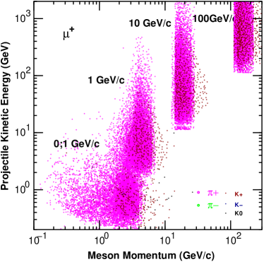
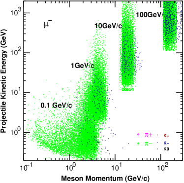
Figure 1: The scatter plot of the projectile and meson momenta, which create 0.1, 1.0, 10 and 100 GeV/c downward moving atmospheric muon at Kamioka (sea level), in the hadronic interaction phase space. We plot those of $\mu^{+}$ in the left panel, and $\mu^{-}$ in the right panel. Note, we use the kinetic energy for the projectile particle in the figure to magnify the region below 1 GeV/c.

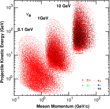
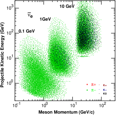
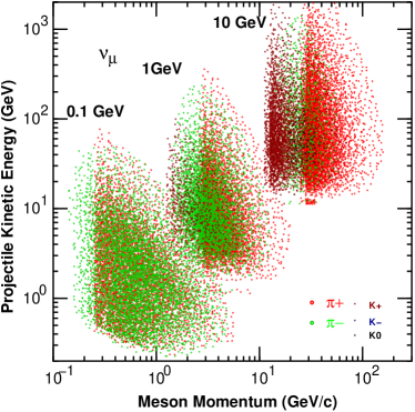
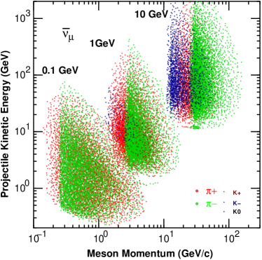
Figure 2: The scatter plot of the projectile and meson momenta, which create the 0.1, 1.0, and 10 GeV vertically downward moving neutrino at Kamioka (sea level), in the hadronic interaction phase space. We plot those of $\nu_{e}$ in the top left panel, $\bar{\nu}_{e}$ in the top right panel, $\nu_{\mu}$ in the bottom left panel and $\bar{\nu}_{\mu}$ in the bottom right panel. Note, we use the kinetic energy for the projectile particle in the figure to magnify the region below 1 GeV/c.

We find the integral kernels for atmospheric neutrino and muon moves almost parallel with their momentum or energy above 1 GeV/c for atmospheric muon and above 1 GeV for atmospheric neutrino. However, the integral kernels for atmospheric muon show a large deformation at 0.1 GeV/c, and the central momentum of the parent meson is very close to the atmospheric muon at 1 GeV. On the other hand, the integral kernel of the atmospheric neutrino at 0.1 GeV shows a little deformation, but keeps the similarity to that of higher energies.

The integral kernel is sensitive not only to the lepton momentum, but also to the direction of the lepton motion, and to the observation site, especially for the atmospheric muon flux. We calculate the integral kernel of atmospheric neutrino flux for vertical downward and horizontal directions at Kamioka, and that of muon flux for vertical downward and horizontal directions at several observation sites including Kamioka.

III variation of the interaction model with random numbers.

If we assume the projectile flux $\Phi_{proj}(N^{proj},p_{N}^{proj},x^{int})$ is not largely affected by the variation of the hadronic interactions, we can study the effect of the variation of the hadronic interactions on the lepton flux using the pseudo-analytic formalism. The lepton flux calculated by the varied interaction model may be written as;

$$\tilde{\Phi}_{L}^{obs}(p_{L}^{obs},x^{obs})= \sum_{N^{proj}}\sum_{M^{born}}\int\int\Big{[}\int M2L(M^{born},p_{M}^{born},x^{int},\ L^{obs},p_{L}^{obs},x^{obs})$$

$$\hskip 56.9055pt\times H_{int}(N^{proj},p_{N}^{proj},x^{int},M^{born},p_{M}^{born})\cdot\left(1+\Delta_{int}(N^{proj},M^{born},p_{N}^{proj},p_{M}^{born})\right)$$

$$\hskip 56.9055pt\times\sigma^{prod}(N^{proj},E^{proj})\cdot\rho_{air}(x^{int})$$

$$\hskip 56.9055pt\times\Phi_{proj}(N^{proj},p_{N}^{proj},x^{int})dx^{int}\Big{]}\ dp_{M}^{born}dp_{N}^{proj}$$ (4)

$$= \sum_{N^{proj}}\sum_{M^{born}}\int\int\ D(N^{proj},p_{N}^{proj},M^{born},p_{M}^{born},\ L^{obs},p_{L}^{obs})$$

$$\hskip 56.9055pt\times\left(1+\Delta_{int}(N^{proj},M^{born},p_{N}^{proj},p_{M}^{born})\right)\ dp_{M}^{born}dp_{N}^{proj}\ .$$ (5)

We can use Eq. 5 to construct a variation of interaction model and the variation of atmospheric lepton fluxes and study it.

The variation of the hadronic interaction model with random numbers can be constructed with the help of the B-spline functions. We use the 3rd order B-spline function with constant knot separation, and is represented as

$$B_{\Delta}^{i}(x)=b\left({{x-i\cdot\Delta}\over\Delta}-x_{0}\right)$$ (6)

where

$$b(t)=\left\{\begin{array}[]{ll}\ \ {1\over 6}(3|t|^{3}-6|t|^{2}+4)&(|t|\leq 1)\\ \\ -{1\over 6}(|t|-2)^{3}&(1\leq|t|\leq 2)\\ \\ \ \ \ 0&(|t|\geq 2)\\ \end{array}\right.\ \ \,$$ (12)

where $\Delta$ is the knot separation, and $x_{0}$ is the origin, normally taken as $x_{0}=0$. The linear combination of the 3rd order B-spline function (Eq. 6 and Eq. 12) is continuous up to the 2nd order derivative, and is often used to connect the discrete data or to fit them.

Using the B-spline function, we construct the variation function as

$$\Delta_{int}(N^{proj},M^{born},p_{N}^{proj},p_{M}^{born})=\delta\cdot\sum_{i}\sum_{j}R_{N}^{ij}\cdot B_{\Delta_{proj}}^{i}(\log_{10}(p_{N}^{proj}))\cdot B_{\Delta_{meson}}^{j}(\log_{10}(p_{M}^{born}))\ ,$$ (13)

Then we can write the variation of lepton flux calculated with this variation of interaction model as,

$$\tilde{\Phi}_{L}^{obs}(p_{L}^{obs},x^{obs})= \sum_{N^{proj}}\sum_{M^{born}}\int\int\ D(N^{proj},p_{N}^{proj},M^{born},p_{M}^{born},\ L^{obs},p_{L}^{obs})$$

$$\hskip 1.42262pt\times\left(1+\delta\sum_{i}\sum_{j}R_{N}^{ij}\cdot B_{\Delta}^{i}(\log_{10}(p_{N}^{proj}))\cdot B_{\Delta}^{j}(\log_{10}(p_{M}^{born}))\right)dp_{M}^{born}dp_{N}^{proj}\ ,$$ (14)

and the variation of the lepton flux as

$$\Delta\Phi_{L}^{obs}(p_{L}^{obs},x^{obs})\equiv \tilde{\Phi}_{L}^{obs}(p_{L}^{obs},x^{obs})-\Phi_{L}^{obs}(p_{L}^{obs},x^{obs})$$

$$= \delta\sum_{N^{proj}}\sum_{M^{born}}\int\int\ D(N^{proj},p_{N}^{proj},M^{born},p_{M}^{born},\ L^{obs},p_{L}^{obs})$$

$$\hskip 14.22636pt\times\sum_{i}\sum_{j}R_{N}^{ij}\cdot B_{\Delta}^{i}(\log_{10}(p_{N}^{proj}))\cdot B_{\Delta}^{j}(\log_{10}(p_{M}^{born}))dp_{M}^{born}dp_{N}^{proj}\ .$$ (15)

Here, we assume $\{R_{N}^{ij}\}$ as the set of normal random numbers with the average value = 0 and the standard deviation = 1, which is one of the standard random number in the computer science. We take $\Delta_{proj}=\Delta_{meson}=\Delta(=0.5)$ in Eq. 14. This means we consider the variation of interaction model in the momentum scale $\Delta\log_{10}(p)\gtrsim 0.5$ both for the projectile and secondary meson momenta.

When the random number set $\{R_{N}^{ij}\}$ is given, the variation of the integral kernel density at a grid point $\{ij\}$ is written as

$$\Delta D_{ij}=D_{ij}\times\delta\sum_{k}\sum_{l}R_{N}^{kl}\cdot B_{\Delta}^{k}((k-i)\cdot\Delta)\cdot B_{\Delta}^{l}((l-j)\cdot\Delta)\ ,$$ (16)

where we have simplified the kernel density at the grid point $D(N^{proj},(p_{N}^{proj})_{i},M^{born},(p_{M}^{born})_{j},\ L^{obs},p_{L}^{obs})$ as $D_{ij}$. Since $\{R_{N}^{kl}\}$ are the set of independent normal random numbers with average value 0, and standard deviation 1, the variance or the square of the standard deviation of $\Delta D_{ij}$ is calculated as

$$\sigma_{D_{ij}}^{2}=D^{2}_{ij}\times\delta^{2}\sum_{k}\sum_{l}\left[B_{\Delta}^{k}((k-i)\cdot\Delta)\cdot B_{\Delta}^{l}((l-j)\cdot\Delta)\right]^{2}\ .$$ (17)

With the definition of B-spline function (Eq. 6 and Eq. 12), the equation is easily evaluated as,

$$\sigma^{\ }_{D_{ij}}=0.5\cdot\delta\cdot D_{ij}\ .$$ (18)

Note, we apply an independent set of random numbers to the integral kernel calculated for each combination of all the projectile and all the secondary meson.

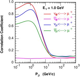
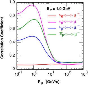
Figure 3: Correlation coefficient for each combination of neutrinos ($\nu_{\mu},\bar{\nu}_{\mu},\nu_{e},\bar{\nu}_{e}$) and muons ($\mu^{+},\mu^{-}$) tat neutrino energy of 1 GeV. We used the integral kernels of atmospheric neutrinos and muons both for vertically downward moving ones at Kamioka.

As an application of the variation of the interaction model with random number, we calculate the correlation coefficient of atmospheric neutrino and atmospheric muon fluxes as,

$$\gamma(p_{\nu}^{obs},x_{\nu}^{obs};p_{\mu}^{obs},x_{\mu}^{obs})={{\sum\left(\Delta\Phi_{\nu}(p_{\nu}^{obs},x_{\nu}^{obs})\Delta\Phi_{\mu}(p_{\mu}^{obs},x_{\mu}^{obs})\right)}\over\sqrt{\sum\left(\Delta\Phi_{\nu}^{k}(p_{\nu}^{obs},x_{\nu}^{obs})\right)^{2}\sum\left(\Delta\Phi_{\mu}^{k}(p_{\mu}^{obs},x_{\mu}^{obs})\right)^{2}}}$$ (19)

and study the correlation coefficient between muon and neuron fluxes at each combination of muon momentum and neutrino energy. As an example, we show the correlation coefficient of neutrino flux at 1 GeV and the muon fluxes as the function of muon momentum in fig. 3 for all combination of ($\nu_{\mu},\bar{\nu}_{\mu},\nu_{e},\bar{\nu}_{e}$) and ($\mu^{+},\mu^{-}$). Here we used the integral kernel of the vertically downward moving fluxes of atmospheric neutrinos and muons at Kamioka. Note, $\pi^{-}$ creates almost all of $\bar{\nu}_{e}$ and $\mu^{-}$, and $\pi^{+}$ creates almost all of $\nu_{e}$ and $\mu^{+}$ in their decay cascade;

$$\pi^{+(-)}\rightarrow \mu^{+(-)}+\nu_{\mu}(\bar{\nu}_{\mu})$$

$$\downarrow$$

$$e^{+(-)}+\bar{\nu}_{\mu}(\nu_{\mu})+\nu_{e}(\bar{\nu}_{e})$$ (20)

at low energies. The correlation coefficient of electron neutrino and muon fluxes created by different types of pion are small and no meaningful structure is seen as the function of muon momentum in Fig. 3. On the other hand, in the case of muon neutrinos, $\pi^{+}$ creates $\nu_{\mu}$, $\bar{\nu}_{\mu}$, and $\mu^{+}$, and $\pi^{-}$ creates $\nu_{\mu}$, $\bar{\nu}_{\mu}$, and $\mu^{-}$. Therefore both signed muon have correlation to both type of muon neutrinos.

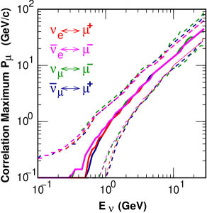
Figure 4: The muon momenta at which the muon show the maximum correlation and the 90% of that to the neutrino at fixed energy (horizontal axis). The left panel is for the neutrinos directly produced at the pion decay, and in the right panel for the neutrinos produced at the decay of muon which produced by the pion decay. We used the integral kernels of vertically downward moving atmospheric neutrinos and muons at Tsukuba or Kamioka (sea level)

In Fig.4, we show the muon momentum which gives the maximum correlation coefficient and 90% of it as the function of neutrino energy for the direct decay product of $\pi^{\pm}$ (left panel) and decay product of $\mu^{\pm}$ (right panel) separately, to see the difference due to the decay kinematics. Note, we do not show the plot for $\nu_{\mu}\leftrightarrow\mu^{-}$ and $\bar{\nu}_{\mu}\leftrightarrow\mu^{+}$, since there are no meaningful correlation between them (Fig. 3). In both the panels, we find the lines for maximum correlation and 90 % of it are very close among different type of the neutrinos, but with the same kinematics.

IV Variation of atmospheric neutrino and muon fluxes

In this section, we generate a huge number (3,000,000) of the normal random number sets, and study the variation of atmospheric neutrino flux when the variation of atmospheric muon flux is limited. To cover a large variation of the interaction model at the beginning, we take $\delta=1$ in Eq.13 in this section. After fixing the kind of target neutrino and it’s energy, we calculate the correlation coefficient of both signed atmospheric muon flux to the target neutrino as the function of the muon momentum. For each signed muon flux, when it has a meaningful correlation maximum, we put the constraint on the flux variation to satisfies the condition;

$$\left|{{\Delta\phi_{\mu}}\over\phi_{\mu}}\right|<\varepsilon\ ,$$ (21)

in the momentum range where the correlation coefficient is larger than the 90 % of the maximum. Therefore, when the target neutrino is electron neutrino ($\nu_{e}$ and $\bar{\nu}_{e}$), the flux variation of either signed muon flux is constrained, and when the target neutrino is muon neutrino ($\nu_{\mu}$ and $\bar{\nu}_{\mu}$), the flux variations of both signed muon fluxes are constrained.

In Fig.5, we plot the variation of $\Delta\Phi_{\nu}/\Phi_{\nu}$ at 1 GeV for $\nu_{e}$ in the left panel and for $\nu_{\mu}$ in the right panel with $\varepsilon=$ 0.1, 0.2, 0.3, and the ones without any constraint ($\varepsilon=\infty$). In this plot, we used the integral kernel for vertically downward moving atmospheric neutrino observed at Kamioka, and the integral kernel for vertically downward moving muon fluxes observed at Kamioka for the illustration.

We find that the distribution of $\Delta\Phi_{\nu}/\Phi_{\nu}$ shrinks in both the panels with the decrease in $\varepsilon$. Considering the interaction model we are using is a variation of the ideal one which gives the real atmospheric neutrino and the muon fluxes, this observation could be interpreted as follows; when our calculated atmospheric muon flux is close to the real one, the atmospheric neutrino flux calculated with the same interaction model must be close to the real one. Furthermore if we consider that the atmospheric muon flux observed by a precision experiment is very close to the real one, we can replace above sentence to; when we can reconstruct the observed atmospheric muon flux observed by a precision experiment, the atmospheric neutrino flux calculated is close to the real one. Note, this arguments are already discussed qualitatively in the other article Sanuki et al. (2007), but this variation study of the hadronic interaction model gives a method for the quantitative discussion.

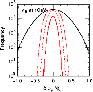
Figure 5: The $\Delta\Phi_{\nu}/\Phi_{\nu}$ distributions for of $\nu_{e}$ flux (left panel) and $\nu_{\mu}$ flux (right panel), created with with Eq. 15 and $\delta=1$, with the 3,000,000 sets of normal random number $\{R_{N}^{ij}\}$ assigned to each grid point. Wide outside solid line shows the distribution with no condition for $\Delta\Phi_{\mu}/\Phi_{\mu}$ ($\varepsilon=\infty$), most inside solid line for $\Delta\Phi_{\mu}/\Phi_{\mu}<0.1$ ($\varepsilon=0.1$), dashed line for $\Delta\Phi_{\mu}/\Phi_{\mu}<0.2$ ($\varepsilon=0.2$), and dotted line for $\Delta\Phi_{\mu}/\Phi_{\mu}<0.3$ ($\varepsilon=0.3$). The integral kernels we used are the vertically downward moving atmospheric neutrinos and muon fluxes at Kamioka.

For each $\varepsilon$, the $\Delta\Phi_{\nu}/\Phi_{\nu}$ distribution is well approximated by the normal distribution as

$$\rho\left(\varepsilon,{\Delta\Phi_{\nu}\over\Phi_{\nu}}\right)={N_{\varepsilon}\over\sqrt{2\pi}}\exp\left({1\over\sigma_{\varepsilon}^{2}}\left({\Delta\Phi_{\nu}\over\Phi_{\nu}}\right)^{2}\right)\ ,$$ (22)

$N_{\varepsilon}$ is the total number of the trial which path the limitation of the variation on the atmospheric muon flux. We note that the distribution without the constraint on the atmospheric muon is also well approximated by the normal distribution then we we use the same distribution formula Eq. 22 with $\varepsilon=\infty$ and $N_{\infty}$, which is the trial number of this study. The concentration of the neutrino flux variation distribution when the variation of atmospheric muon flux is constrained with $\varepsilon$ may be studied by the ratio of ${\rho\left(\varepsilon,{\Delta\Phi_{\nu}/\Phi_{\nu}}\right)}$ and $\rho\left(\infty,{\Delta\Phi_{\nu}/\Phi_{\nu}}\right)$, after the normalization as,

$$\left[{1\over N_{\varepsilon}}{\rho\left(\varepsilon,{\Delta\Phi_{\nu}\over\Phi_{\nu}}\right)}\right]/\left[{1\over N_{\infty}}\rho\left(\infty,{\Delta\Phi_{\nu}\over\Phi_{\nu}}\right)\right]=\exp\left(\left({1\over\sigma_{\varepsilon}^{2}}-{1\over\sigma_{\infty}^{2}}\right)\cdot\left({\Delta\Phi_{\nu}\over\Phi_{\nu}}\right)^{2}\right)$$ (23)

Therefore, we define the concentration parameter $\sigma_{shrink}$ as

$${1\over{\sigma_{shrink}^{2}}}={1\over{\sigma^{2}({\varepsilon})}}-{1\over{\sigma_{\infty}^{2}}}\ \ \ ,$$ (24)

$\sigma_{shrink}$ would be the standard deviation of the atmospheric neutrino flux variation, when the original distribution of it is flat, and the variation of atmospheric muon flux is restricted by Eq. 21.

Let us consider the variation of atmospheric neutrino flux is the combination of two components; one is independent of that of atmospheric muon flux, and the other is related to that of atmospheric muon flux. When $\varepsilon$ approaches 0 in Eq. 21, the remaining variation of atmospheric neutrino flux would be the component independent of the atmospheric muon flux. We assume a simple function form for $\varepsilon$ and $\sigma_{shrink}$ as

$$\sigma_{shrink}=\sqrt{\varsigma_{0}^{2}+\left(\varsigma_{1}\cdot\varepsilon\right)^{2}}\ \ ,$$ (25)

where $\varsigma_{0}$ represents the atmospheric neutrino flux variation independent of the atmospheric neutrino flux, and $\varsigma_{1}\cdot\varepsilon$ the atmospheric neutrino flux variation related to the atmospheric muon flux.

Adding a little more data points, we fit the $\sigma_{shrink}$ with Eq. 25 for the atmospheric neutrino variation distribution shown in Fig. 5, and show the best fit curves for $\nu_{e}$ (left panel) and $\nu_{\mu}$ (right panel). We find Eq. 25 fit well both data, and $\sigma_{shrink}$ is already very close to the $\varsigma_{0}$ at $\varepsilon\sim 0.05$. Note, we intend to apply this analysis to find a better interaction model for the calculation of atmospheric neutrino flux by the reconstruction test of the atmospheric muon flux observed by a precision experiment. Then $\Delta\phi_{\mu}/\phi_{\mu}\lesssim 0.05$ would be the practical target in this test.

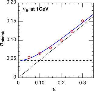
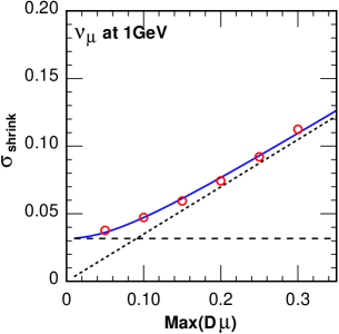
Figure 6: The $\sigma_{shrink}$ obtained by the variation study of atmospheric neutrino flux for vertically downward moving atmospheric electron neutrino and downward moving atmospheric muon fluxes at Kamioka. for $\varepsilon$ = 0.5, 1.0, 1.5, 2.0, 2.5 and 3.0. The solid curve shows the best fit curve with Eq. 25, and the dash and dotted lines show two asymptotic lines of Eq. 25; $\sigma_{shrink}=\varsigma_{0}$, and $\sigma_{shrink}=\varsigma_{1}\cdot\varepsilon$. We show those for $\nu_{e}$ in the left panel, and for $\nu_{\mu}$ in the right panel.

Using the integral kernel for vertically downward moving atmospheric muon flux at Kamioka, we repeat the variation study with $\varepsilon$ = 0.5, 1.0, 1.5, 2.0, 2.5 and 3.0, and fit the resulting $\sigma_{shrink}$ by Eq. 25 to determine $\varsigma_{0}$ or the muon independent component of the atmospheric neutrino flux variation, for vertically downward and horizontally moving atmospheric neutrino fluxes at Kamioka in the energy range from 0.1 GeV to 100 GeV beyond our target, and for all kind of neutrinos. We plot the $\varsigma_{0}$ in Fig. 7 as the function of neutrino energy. Note, we set the minimum muon momentum for this study to 0.1 GeV$/$c. This means that we study the correlation coefficient of neutrino and muon fluxes in the muon momentum range larger than 0.1 GeV$/$c for a given neutrino energy. Then we constrain the muon flux variation at the muon momentum where the correlation coefficient is larger than the 90 % of the maximum.

The most crucial fact in Fig. 7 is that $\varsigma_{0}$ increases rapidly as the neutrino energy decrease below 1 GeV, for all the kind of neutrinos. In the next section, we will discuss on the rise of $\varsigma_{0}$ at low energies. Although the energy region is out of our target energy region, we have some comments on the $\varsigma_{0}$ increase with neutrino energy above a few GeV. This is due to the kaon contribution to neutrino production, whose variation is not restricted by the limitation of the variation of the atmospheric muon flux. As the kaon contribution is largest to $\nu_{\mu}$ production among all the neutrinos, the $\varsigma_{0}$ increase of $\nu_{\mu}$ is largest among them. Note, we have also assumed the uncertainty of kaon production is 50 % at the every grid point of the integral kernel in Eq. 15. If we apply here the uncertainty of kaon production by accelerator experiment, the increase of $\varsigma_{0}$ would be suppressed. For the horizontally moving neutrinos, still the increase of $\varsigma_{0}$ is seen for $\nu_{\mu}$, but generally it stays $\lesssim 0.05$ below 100 GeV.

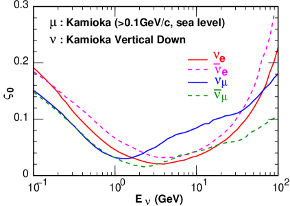
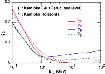
Figure 7: The $\varsigma_{0}$ or the atmospheric muon independent variation component of neutrino flux, calculated with the muon flux integral kernel for the vertically downward moving atmospheric muon flux at Kamioka (sea level). The minimum muon momentum is set to 0.1 GeV$/$c. In the left panel, we depicted the $\varsigma_{0}$ for vertical downward moving atmospheric neutrino at Kamioka, and in the right panel for horizontal moving atmospheric neutrino at Kamioka.

V analysis of existing data

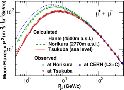
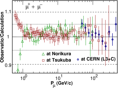
Figure 8: Left panel: vertically downward atmospheric muon flux ($\mu^{+}+\mu^{-}$ ) observed by the BESS detector at Tsukuba (sea level, squares) Haino et al. (2004) and at M. Norikura (2770m a.s.l., upper triangles) Sanuki et al. (2002), by L3+C experiment Achard et al. (2004) at CERN (circles). Solid line is the vertically downward atmospheric muon flux calculated for Tsukuba, dashed line for Mt. Norikura, dotted line for Hanle (4500m a.s.l. India). Right panel: Expanded comparison of observation and calculation taking their ratio.

In our former study Sanuki et al. (2007), we have estimated our calculation error for the atmospheric neutrino flux using the atmospheric muon spectra observed by the BESS detector at Tsukuba (sea level) Haino et al. (2004), at Mt. Norikura (2770m a.s.l.) Sanuki et al. (2002) above 0.567 GeV$/$c. In the left panel of Fig. 8, we plot these data taking the flux sum of $\mu^{+}$ and $\mu^{-}$ with the data observed by L3+C experiment Achard et al. (2004) at CERN. We also depict the calculated fluxes for these observation sites, and for Hanle (India, 4500m a.s.l.) in the same figure. In the right panel of Fig. 8, we show the comparison of observed and calculated atmospheric muon flux expanding the difference by taking the ratio. Note, we have renewed the calculation of the muon flux with the primary cosmic ray model based on AMS02 and other precision measurements Aguilar et al. (2015a, b); Adriani et al. (2013); Abe et al. (2017).

We apply the study in the previous section to these data, especially to those observed by BESS. Note, the agreement of calculation and the observed data for atmospheric muon flux is generally good and the reconstruction residual is less than 5 % above 1 GeV. However, below 1 GeV, we failed to reconstruct the observed muon flux at Tsukuba and at Mt. Norikura at the same time. Probably we need new observation by a precision experiment, dedicated to the low momentum muon flux ($\lesssim$ 1 GeV). In the previous section, we calculate $\varsigma_{0}$ with the minimum muon momentum of 0.1 GeV$/$c (Fig. 7), implicitly assuming that we can reconstruct the the accurately measured muon flux for $P_{\mu}\gtrsim$ 0.1 GeV$/$c. In the previous section, we have calculate the $\varsigma_{0}$ with the integral kernel for the vertically downward moving atmospheric muon flux at Kamioka, where the muon observation condition is very close to Tsukuba, and here we re-calculate it and plot in Fig. 9 with a little change that the minimum muon momentum is set to be 1 GeV$/$c. Note, we plot the $\varsigma_{0}$ rather than the $\sigma_{shrink}$ with the residual shown in the left panel of Fig. 8, since the estimation of residual at each momentum is difficult due to the muon flux observation error, but it would be smaller than 0.05 in Fig. 8. Note, $\sigma_{shrink}$ at $\varepsilon$=0.05 is very close to $\varsigma_{0}$.

The $\varsigma_{0}$ or the atmospheric muon independent variation component of neutrino flux in Fig. 9 is compared with that in Fig. 7, and we find the $\varsigma_{0}$ in Fig. 9 shows a quicker increase towards lower energy below 1 GeV, but it is very similar in each figure above $\sim$ 1 GeV. We may say that, using the atmospheric muon data observed by BESS at Mt. Norikura, we can draw almost the same conclusion on the uncertainty of the low energy atmospheric neutrino flux as that in Ref. Sanuki et al. (2007).

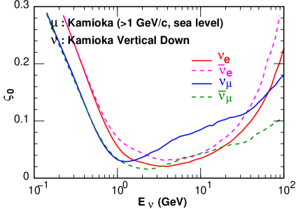
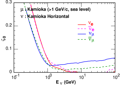
Figure 9: The $\varsigma_{0}$ or the atmospheric muon independent variation component of neutrino flux, calculated with the muon flux integral kernel for the vertically downward moving atmospheric muon flux at Kamioka (sea level). The minimum muon momentum is set to 1 GeV$/$c. In the left panel, we depicted the $\varsigma_{0}$ for vertical downward moving atmospheric neutrino at Kamioka, and in the right panel for horizontal moving atmospheric neutrino at Kamioka.

VI Survey of muon observation site for future experiments

In the previous section we applied the study in Sec. IV to the presently available data. We could confirm the result of our former study, but also find we need more muon flux data with a precision experiment dedicated to lower muon momentum. However, the comparison of Fig.  7 and Fig. 9, tells us that, just by lowering the minimum muon momentum, it is difficult to reduce the uncertainty of low energy atmospheric neutrino flux largely with the muon observation at sea level. Then we look for suitable muon observation site for the future atmospheric muon observation experiment. Considering the progress of the detectors used in the recent cosmic ray o observations, we assume that we can get the accurate muon flux data from 0.3 GeV$/$c in a precision experiment for the low energy muon flux observation.

Let us start the survey from Tsukuba (sea level), where BESS group has observed the muon flux as we stated in the previous section. In Fig.  10, we plot $\varsigma_{0}$ for the atmospheric neutrino flux at Kamioka, with the integral kernel for the vertical downward moving atmospheric muon flux at Tsukuba (sea level). Since the observation altitude and the rigidity cutoff are very close to those at Kamioka, we can compare this result with those presented and discussed in the previous section. We find the result here is in between of those with the minimum muon momentum of 0.1 GeV$/$c (Fig. 7) and of 1 GeV$/$c (Fig. 9), and is rather close to the calculation with minimum momentum of 0.1 GeV$/$c. Therefore, if the atmospheric muon flux is measured down to 0.3 GeV$/$c, by a precision experiment, it will improve the result with former BESS observation and constrain the uncertainty in the atmospheric neutrino flux down to a little less than 1 GeV.

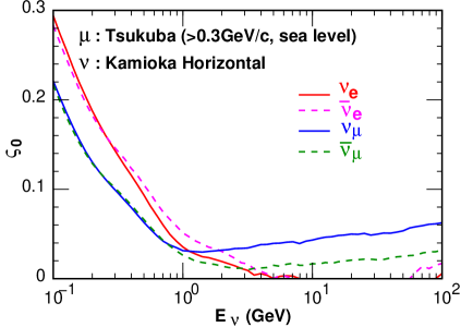
Figure 10: The $\varsigma_{0}$ or the atmospheric muon independent variation component of neutrino flux, calculated with the muon flux integral kernel for the vertically downward moving atmospheric muon flux at Tsukuba (sea level). The minimum muon momentum is set to 0.3 GeV$/$c. In the left panel, we depicted the $\varsigma_{0}$ for vertical downward moving atmospheric neutrino at Kamioka, and in the right panel for horizontal moving atmospheric neutrino at Kamioka.

Next we move to Mt. Norikura (2770m a.s.l.), where BESS group also has observed the muon flux. In Fig.  10, we plot $\varsigma_{0}$ for the atmospheric neutrino flux at Kamioka, with the integral kernel for the vertical downward moving atmospheric muon flux at Mt. Norikura (2770m a.s.l.l), and the minimum muon moment of 0.3 GeV$/$c. We find the $\varsigma_{0}$ at Mt. Norikura is similar to that at Tsukuba for $E_{\nu}>0.5$ GeV, but show a large reduction for $E_{\nu}<0.5$ GeV. It is remarkable that $\varsigma_{0}<0.1$ is satisfied for each kind of neutrino in 0.3 GeV $<E_{\nu}<$ 10 GeV for vertical direction and in $E_{\nu}>0.3$ GeV for horizontal direction. Thus the observation at the high altitude is seems to have an advantage in the reduction of the uncertainty of the low energy neutrino flux prediction.

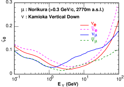
Figure 11: The $\varsigma_{0}$ or the atmospheric muon independent variation component of neutrino flux, calculated with the muon flux integral kernel for the vertically downward moving atmospheric muon flux at Mt. Norikura (2770m a.s.l.). The minimum muon momentum is set to 0.3 GeV$/$c. In the left panel, we depicted the $\varsigma_{0}$ for vertical downward moving atmospheric neutrino at Kamioka, and in the right panel for horizontal moving atmospheric neutrino at Kamioka.

As it seems the higher altitude is more suitable for the muon observation site, we look for a candidate at much higher altitude, and find Hanle (4500m a.s.l., India) han satisfies the condition, where the Indian astronomical observatory exists. We calculate the $\varsigma_{0}$ for the atmospheric neutrino flux at Kamioka, with the integral kernel for vertical downward moving atmospheric muon at Hanle, and plot it In Fig.  12 . The minimum muon momentum is set to 0.3 GeV$/$c as before. Comparing with the $\varsigma_{0}$ calculated with the muon at Mt. Norikura, we find the the $\varsigma_{0}$ for Hanle is generally smaller in $E_{\nu}<1$ GeV. Especially $\varsigma_{0}<0.1$ is satisfied in $0.15<E_{\nu}<10$ GeV for all the kind of neutrino and for all the directions.

The last candidate for muon observation site is the balloon which is used for the observation of primary cosmic rays. Note, we have once used the balloon altitude muon data observed by BESS Abe et al. (2003) to study the interaction model at low energies Honda et al. (2011). However, we could not conclude a strong statement due to the poor statistics. We calculate the $\varsigma_{0}$ for the atmospheric neutrino flux at Kamioka with the integral kernel for the vertical downward moving atmospheric muon at Balloon altitude (32km a.s.l., near south pole), and plot it in Fig.  13. Note, as the atmospheric muon flux at balloon altitude is small than the lower altitudes, we consider a long flight balloon experiment for the observation of it. The minimum muon momentum is set 0.3 GeV$/$c as before. We find that the value of $\varsigma_{0}$ is larger than those of others in the all neutrino energy region we studied. This means the muon observation at balloon altitude does not reduce the uncertainty of the low energy atmospheric neutrino flux more than that on a high mountain. We have to look for a good muon observation site on a high mountain.

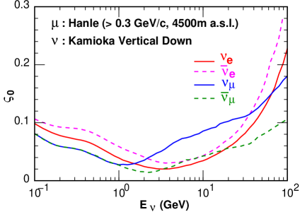
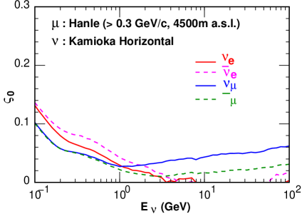
Figure 12: The $\varsigma_{0}$ or the atmospheric muon independent variation component of neutrino flux, calculated with the muon flux integral kernel for the vertically downward moving atmospheric muon flux at Hanle (4500m a.s.l.). The minimum muon momentum is set to 0.3 GeV$/$c. In the left panel, we depicted the $\varsigma_{0}$ for vertical downward moving atmospheric neutrino at Kamioka, and in the right panel for horizontal moving atmospheric neutrino at Kamioka.

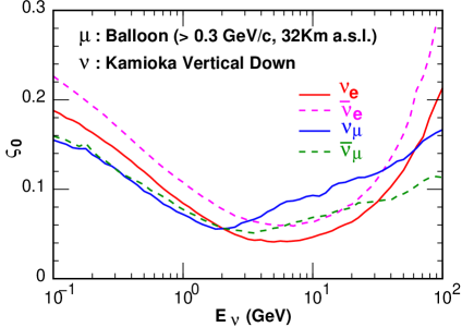
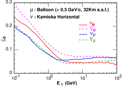
Figure 13: The $\varsigma_{0}$ or the atmospheric muon independent variation component of neutrino flux, calculated with the muon flux integral kernel for the vertically downward moving atmospheric muon flux at Balloon altitude (32km a.s.l.). The minimum muon momentum is set to 0.3 GeV$/$c. In the left panel, we depicted the $\varsigma_{0}$ for vertical downward moving atmospheric neutrino at Kamioka, and in the right panel for horizontal moving atmospheric neutrino at Kamioka.

VII Uncertainties of the Projectile flux and the scattering angle

In Sec. III, we assumed that the projectile flux $\Phi_{proj}(N^{proj},p_{N}^{proj},x^{int})$ is not largely affected by the variation of the hadronic interactions. We would like to comment on this assumption and the uncertainty due to it. Classifying the projectile particles of the hadronic interaction with air nuclei into three types, proton, neutron, and all as mesons as in Sec. II, we plot the fraction of them for when their hadronic interaction resulted in the target lepton production in Fig. 14, summing all kind of neutrinos in the left panel, and summing both signed muons in the right panel.

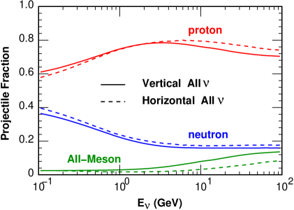
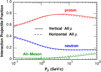
Figure 14: Left panel; relative ratio of projectile particle ratio for vertical downward and horizontally moving atmospheric neutrino calculated for Kamioka summing all kind of neutrinos. Right panel; relative ratio of projectile particle ratio for vertical downward moving atmospheric muon calculated for Kamioka, summing both signed muons.

The primary cosmic ray energy which produce the atmospheric neutrino and muon fluxes we are studying is less than a few TeV, and the proton neutron ratio ($N_{p}/N_{n}$) is around 5. However, from Fig,. 14, we find the $N_{p}/N_{n}$ ratio of the projectile particle directly related to those atmospheric neutrino and muon fluxes is 1.5 at the lowest energy and around 4 in the highest energy of our study in this paper. This means that some of the projectile particle have experienced hadronic interaction before they create the parent meson of the atmospheric neutrino and muon. The small $N_{p}/N_{n}$ ratio at low energies means they are created by the projectiles which suffered more from the hadronic interaction than the atmospheric neutrino and muon at higher energies.

As the contribution of mesons projectile is small for atmospheric neutrino and muon below 100 GeV, we consider here the variation of $N_{p}/N_{n}$ ratio only. We repeat the study in section IV, changing the $N_{p}/N_{n}$ ratio by $\pm 10$ % for the atmospheric muon but fixing it to the original value for the atmospheric neutrino, and fixing the $N_{p}/N_{n}$ ratio to the original value for the atmospheric muon but changing it by $\pm 10$ % for the atmospheric neutrino by hand. With those changes, we find the peak position of $\Delta\Phi_{\nu}/\Phi_{\nu}$ distribution moves only $\pm 2\sim 3$ %, which is would not be seen clearly if we add the distribution in Fig. 5. Note, the same change of $N_{p}/N_{n}$ ratio for the atmospheric muon and atmospheric neutrino shift the peak position to the opposite direction. Considering the fact that a variation of hadronic interaction model would change the $N_{p}/N_{n}$ ratios for the atmospheric neutrino and muon fluxes to the same direction, we may conclude that the possible variation of the projectile particle ratio with the variation of hadronic interaction model does not affect the former section analysis largely.

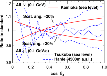
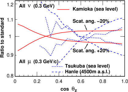
Figure 15: The flux ratios of atmospheric neutrino and muon calculated with 20% larger and 20% smaller scattering angle to that with standard scattering angel in our calculation scheme at several sites. The solid lines are for the ratios of atmospheric neutrino flux calculated at Kamioka, dashed lines are the ratio of atmospheric muon flux calculated at Hanle, and dotted lines are the ratio of atmospheric muon flux calculated at Tsukuba. Left panel is for the atmospheric neutrino at $E_{\nu}=0.1$ GeV, and atmospheric muon with momentum at $P_{\mu}=0.1$ GeV$/$c. Right panel is for the atmospheric neutrino at $E_{\nu}=0.1$ GeV and atmospheric muon at $P_{\mu}=0.1$ GeV$/$c.

Another potentially important source of the uncertainty for the lower energy atmosphere neutrino flux is the error of the scattering angle in the hadronic interaction. It is well known that the three-dimensional calculation of atmospheric neutrino flux shows an enhancement of the flux for near horizontal directionsBattistoni et al. (2003), and is sometimes called the “horizontal enhancement”. This is due to the bending of secondary particles from the projectile particle in the hadronic interaction, and is not seen in the one-dimensional calculations. Therefore, the error in the measurement of the scattering angle could result in the error of the prediction of the low energy atmospheric neutrino flux.

To quantify the uncertainty of the atmospheric neutrino flux due to the error in the scattering angle in the hadronic interaction, we calculate the atmospheric neutrino flux at Kamioka and muon flux at several observation sites changing the scattering angles of the hadronic interaction model to $\pm$20 % larger or smaller ones by hand. Summing all kind of neutrino flux calculated at Kamioka, we plot the ratio of the scattering angle changed neutrino fluxes to the original one as the function of zenith angle at $E_{\nu}=0.1$ GeV (left panel) and at $E_{\nu}=0.3$ GeV (right panel) in Fig. 15. We also sum the flux of both signed atmospheric muon calculated at Tsukuba and Hanle, and plot the ratio of the scattering angle changed muon fluxes to the original one as the function of zenith angle at $P_{\mu}=0.1$ GeV$/$c (left panel) and at $P_{\mu}=0.3$ GeV$/$c (right panel) in Fig. 15. We find $\sim\pm$ 10 % variation for the scattering angle changed neutrino flux at the near horizontal direction in both energy, and for vertically downward direction at 0.1 GeV. Therefore, if we want to reduce the error in the calculation of atmospheric neutrino to $\sim$ 5 %, we need to reduce the uncertainty of the hadronic interaction scattering angle to $\lesssim$ 10 %. At the same time, We also observe that the same change of the scattering angle also cause a large the change in the zenith angle dependence of atmospheric muon flux observed at high altitude site as Hanle (4500m a.s.l.), but a smaller change at sea level (Tsukuba). The muon observed at higher altitude as Hanle, whose the production altitude is close to the observation altitude, are a little suffered from the muon energy loss, and the change of scattering angle appears as a large effect on the zenith angle dependence of muon flux. On the other hand, the muon observed at the sea level suffer the maximum energy loss, and the observed zenith angle dependence is that of higher energy one, where the change of the scattering angle appears smaller effect on the zenith angle dependence of muon flux.

The precision measurement of the scattering angle in the hadronic interaction is the work of accelerator experiments. However, the Fig. 15 shows a possibility to study the uncertainty of it by measuring the atmospheric muon flux as the function of the zenith angle. We note that this observation must be carried out at high mountain like Hanle (4500m a.s.l.). As the atmospheric muon flux decreases quickly with the zenith angle, the larger flux is preferable for this observation. We expect $\sim$ 4 times larger atmospheric muon flux at Hanle than that at sea level (see Fig. 8), Also the effect of the variation of the scattering angle is more visible in the atmospheric muon flux data observed at higher mountain. We may reduce the uncertainty of the scattering angle in hadronic interaction, by reconstructing the atmospheric muon flux accurately observed at Hanle.

VIII Summary and Conclusions

Based on the pseudo-analytic formulation for the calculation of the atmospheric lepton flux, we developed a method to construct the variation of hadronic interaction model with the random numbers. Then we construct a huge number of the variation of the interaction model and the variation of atmospheric neutrino and muon flux with them. We find that when we select the variation of interaction models whose calculated atmospheric muon fluxes is close to the original one, the atmospheric neutrino flux calculated with that is also close to the original one. By considering our interaction model, with which we are calculating the atmospheric neutrino and muon fluxes, is a variation of the ideal interaction model which can predict the true atmospheric neutrino and muon fluxes, we may conclude that when we can reconstruct the atmospheric muon flux measured by a precision experiment, we can also calculate the atmospheric neutrino flux accurately.

Note, in our former studies, we modify the hadronic interaction model and reconstruct the accurately measured atmospheric muon flux in a good accuracy. However, the study of this paper shows that there remains some uncertainty of the atmospheric neutrino flux depending on the observation site and the minimum momentum of the atmospheric muon flux data rather than on the residual of the reconstruction. It is important to improve the muon observation equipment and find a better observation site for atmospheric muon flux. We hope the technology used in the recent primary cosmic ray observation detectors would improve also the muon observation detectors. For the observation site, we find that the atmospheric muon flux data observed at high mountain is better than that observed at a lower altitude site, to reduce the uncertainty of the atmospheric neutrino flux. It seems the mountain site (3000 $\sim$ 5000 m a.s.l.) works most efficiently for this work, because the remaining uncertainty decrease with the altitude of the observation site up to 4500 m a.s.l., but if we go up to the balloon altitude ($\sim$ 32 km), the remaining uncertainty rather increases.

As other source of the uncertainty of the atmospheric neutrino calculation, we considered the uncertainty of the projectile particle flux for the hadronic interaction which create the parent meson of the atmospheric neutrino and muon. We studied it by changing the relative ratio of the kind of projectile particles in the above variation study of the interaction model. However, the result is virtually the same. This is because the variation study of the hadronic interaction model cover the variation of the projectile particles flux.

We observed that the uncertainty of the scattering angle in hadronic interaction is also the source of uncertainty of the low energy atmospheric neutrino flux prediction due to the horizontal enhancement. This could be crucial to the study of neutrino physics, since this uncertainty result in the uncertainty in the zenith angular distribution of atmospheric neutrino flux. To study this uncertainty, we calculated the atmospheric neutrino flux, assuming the variation of the scattering angle by $\pm 20$ %, and we find the flux difference is $\lesssim$ 10 % at 0.1 GeV and 0.3 GeV, both for the vertical downward and horizontal direction. If we reduce the uncertainty of the scattering angle in the hadronic interaction to $\lesssim$ 10 %, the uncertainty of atmospheric neutrino would be $\lesssim$ 5 %. The uncertainty of the scattering should be studied at the accelerator experiment, but the study of atmospheric muon zenith angle variation at high mountain altitude as Hanle, the atmospheric muon observation can also contribute to reduce it.

Lastly, we would like to comment on the relation of our work and accelerator experiment in the calculation of the atmospheric neutrino flux. First of all, we must confess that the interaction model we are using is basically constructed using the accelerator data. Without the acceleration experiments, we could not start the calculation of the atmospheric neutrino flux. We would like to note that the accelerator experiment can improve the study of this paper, the reduction of the uncertainty of atmospheric neutrino flux using the accurately measured muon flux, We have assumed 50 % uncertainty in the integral kernel density at each grid point for all kind of hadronic interaction related to the atmospheric neutrino and muon production. If we can start with much smaller uncertainty for the integral kernels, the remaining uncertainty would be smaller. Although it is a higher energy problem, the kaon production uncertainty is typically this case. We believe the cooperation with accelerator study is necessary to achieve much higher accuracy in the prediction of the atmospheric neutrino flux.