Number and location of pre-images under harmonic mappings in the plane

Abstract

We derive a formula for the number of pre-images under a non-degenerate harmonic mapping $f$, using the argument principle. This formula reveals a connection between the pre-images and the caustics. Our results allow to deduce the number of pre-images under $f$ geometrically for every non-caustic point. We approximately locate the pre-images of points near the caustics. Moreover, we apply our results to prove that for every $k=n,n+1,\ldots,n^{2}$ there exists a harmonic polynomial of degree $n$ with $k$ zeros.

Keywords:

Harmonic mappings, pre-images, caustics, argument principle, valence, zeros of harmonic polynomials.

AMS Subject Classification (2010):

30C55; 31A05; 55M25.

1 Introduction

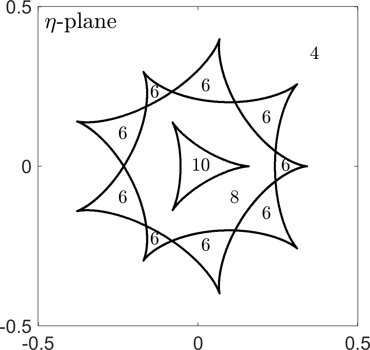
Figure 1: Number of pre-images of $\eta$ under $f(z)=z-\overline{z^{2}/(z^{3}-0.6^{3})}$ for an $\eta$ in the respective regions; see also Example 3.9 below. The black lines mark the caustics (critical values) of $f$. The number of pre-images of $\eta$ in the outer tile corresponds to the number of poles of $f$ (including $\infty$).

Harmonic mappings in the plane, i.e., functions $f:\Omega\to\mathbb{C}$ with $\Delta f=0$ on an open set $\Omega\subseteq\mathbb{C}$, regained attention in the last decades, starting from the seminal work of Clunie and Sheil-Small [10]. See, e.g., the large collection of open problems by Bshouty and Lyzzaik [9] and references therein. While we consider here multivalent harmonic mappings, also (locally) univalent harmonic mappings are of interest, see, e.g., Duren’s textbook [11], especially in the context of quasi-conformal mappings [1].

Numerous authors have studied the number and location of zeros of harmonic mappings, i.e., the solutions of $f(z)=0$. Of particular interest have been harmonic polynomials of the form $f(z)=p(z)-\overline{z}$ [19, 13], or $f(z)=p(z)+\overline{q(z)}$ and the questions related to Wilmshurst’s conjecture [38, 20, 16]. Also, the zeros of rational harmonic mappings of the form $f(z)=r(z)-\overline{z}$ have been studied intensively [17, 7, 25, 26, 22], since these are of interest when modeling the phenomenon of gravitational lensing [18, 29, 5].

Here we focus on solutions of $f(z)=\eta$ for given (but arbitrary) $\eta\in\mathbb{C}$. As shown in [21] for rational harmonic mappings of the form $f(z)=r(z)-\overline{z}$, the number of solutions can vary significantly under changes of $\eta$. Moreover, changes only occur when $\eta$ is “moved” through the caustics of $f$; see Figure 1. This paper is devoted to study this effect for a more general class of harmonic mappings. We show the following:

(1) In Section 3 we derive (local and global) formulas for the number of pre-images of $\eta$ under a non-degenerate harmonic mapping $f$ (Definition 3.1) in terms of the poles and the winding number of the caustics about $\eta$, e.g.,

$$N_{\eta}(f)=P(f)+2\sum_{\gamma\in\operatorname{crit}}n(f\circ\gamma;\eta);$$ (1.1)

see Theorem 3.4. An immediate consequence of (1.1) is that the number of pre-images changes by $\pm 2$ when $\eta$ changes from one side to the other of a single caustic arc; see Figure 1.

(2) In Section 4 we complement Lyzzaik’s study [27] of the local behavior of light harmonic mappings at their critical points. We approximately locate pre-images of $\eta$ near a fold caustic point, which makes the pre-images also accessible for computations. Moreover, we determine for which $\eta$ near a fold we have locally two or no pre-images; see Theorem 4.2.

(3) In Section 5 we apply the results from Sections 3 and 4 to harmonic polynomials. In particular we prove that for all $k\in\{n,n+1,\ldots,n^{2}\}$ there exists a harmonic polynomial $f(z)=p(z)+\overline{q(z)}$ with $\deg(p)=n$ and $\deg(q)<n$ with exactly $k$ zeros, i.e., every number between the minimum and maximum can be attained; see Corollary 5.6. This generalizes a result of Bleher et al. [7, Thm. 1.1].

2 Preliminaries

The key ingredient to derive the formulas for the exact number of pre-images in Section 3 is the argument principle for harmonic mappings, applied on the critical set. In preparation, we collect and extend several known results in this section.

A harmonic mapping is a function $f:\Omega\to\mathbb{C}$ defined on an open set $\Omega\subseteq\mathbb{C}$ and with

$$\Delta f=\partial_{xx}f+\partial_{yy}f=4\partial_{\overline{z}}\partial_{z}f=0,$$

where $\partial_{z}$ and $\partial_{\overline{z}}$ denote the Wirtinger derivatives of $f$; see e.g. [11, Sect. 1.2]. If $f$ is harmonic in the open disk $D=\{z\in\mathbb{C}:\lvert z-z_{0}\rvert<r\}$, it has a local decomposition

$$f(z)=h(z)+\overline{g(z)}=\sum_{k=0}^{\infty}a_{k}(z-z_{0})^{k}+\overline{\sum_{k=0}^{\infty}b_{k}(z-z_{0})^{k}},\quad z\in D,$$ (2.1)

with analytic functions $h$ and $g$ in $D$, which are unique up to an additive constant; see [12, p. 412] or [11, p. 7]. If $f$ is harmonic in the punctured disk $D=\{z\in\mathbb{C}:0<\lvert z-z_{0}\rvert<r\}$, it has a local decomposition

$$f(z)=\sum_{\mathclap{k=-\infty}}^{\infty}a_{k}(z-z_{0})^{k}+\overline{\sum_{\mathclap{k=-\infty}}^{\infty}b_{k}(z-z_{0})^{k}}+c\log\lvert z-z_{0}\rvert,\quad z\in D;$$ (2.2)

see [35, 14]. We consistently use the notation from (2.1) and (2.2).

The Jacobian of a harmonic mapping $f$ at $z\in\Omega$ is

$$J_{f}(z)=\lvert\partial_{z}f(z)\rvert^{2}-\lvert\partial_{\overline{z}}f(z)\rvert^{2}=\lvert h^{\prime}(z)\rvert^{2}-\lvert g^{\prime}(z)\rvert^{2},$$ (2.3)

where $f=h+\overline{g}$ is a local decomposition (2.1). We call $f$ sense-preserving at $z$ if $J_{f}(z)>0$, sense-reversing at $z$ if $J_{f}(z)<0$, and singular at $z$ if $J_{f}(z)=0$. Moreover, we call $f$ singular, if $f$ is singular at one of its zeros. If $\varphi$ is an analytic function, then $f\circ\varphi$ is again a harmonic mapping and

$$J_{f\circ\varphi}(z)=J_{f}(\varphi(z))\lvert\varphi^{\prime}(z)\rvert^{2}.$$ (2.4)

In particular, if $\varphi^{\prime}(z)\neq 0$, the maps $f$ at $\varphi(z)$ and $f\circ\varphi$ at $z$ are simultaneously sense-preserving, sense-reversing, or singular, respectively.

2.1 Critical set and caustics

The points at which a harmonic mapping $f$ is singular form the critical set

$$\mathcal{C}=\{z\in\Omega:J_{f}(z)=0\},$$ (2.5)

which consists of the level set of an analytic function, and certain isolated points, as we see next.

The second complex dilatation of a harmonic mapping $f$ is

$$\omega(z)=\frac{\overline{\partial_{\overline{z}}f(z)}}{\partial_{z}f(z)}=\frac{g^{\prime}(z)}{h^{\prime}(z)},$$

with the decomposition $f=h+\overline{g}$ from (2.1); see [11, p. 5], [1, p. 5] or [35, p. 71]. We assume that $\partial_{z}f=h^{\prime}$ has only isolated zeros in $\Omega$, so that $\omega$ is analytic in $\{z\in\Omega:\partial_{z}f(z)\neq 0\}$, and the singularities of $\omega$ in $\Omega$ are poles or removable singularities (which we assume to be removed). Moreover, we assume that $\lvert\omega\rvert\not\equiv 1$ on an open set (harmonic mappings with this property are characterized in [27, Lem. 2.1]).

Let $z_{0}\in\Omega$. If $h^{\prime}(z_{0})\neq 0$, then $J_{f}(z_{0})=\lvert h^{\prime}(z_{0})\rvert^{2}-\lvert g^{\prime}(z_{0})\rvert^{2}=0$ is equivalent to $\lvert\omega(z_{0})\rvert=1$, and if $h^{\prime}(z_{0})=0$, then $J_{f}(z_{0})=0$ is equivalent to $g^{\prime}(z_{0})=0$. Hence, $\lvert\omega(z_{0})\rvert=1$ implies $J_{f}(z_{0})=0$, but the converse is not true in general. Define

$$\mathcal{M}=\{z\in\mathcal{C}:\lvert\omega(z)\rvert\neq 1\}.$$ (2.6)

By the above computation,

$$\mathcal{M}=\{z\in\Omega:h^{\prime}(z)=g^{\prime}(z)=0\text{ and }\lim_{\zeta\to z}\lvert\omega(\zeta)\rvert\neq 1\}.$$

For $z_{0}\in\mathcal{M}$, there exists a neighborhood of $z_{0}$ containing no other point in $\mathcal{C}$; see [27, Lem. 2.2]. By construction,

$$\mathcal{C}\setminus\mathcal{M}=\{z\in\Omega:\lvert\omega(z)\rvert=1\}$$

is a level set of the analytic function $\omega$. Hence, $\mathcal{C}\setminus\mathcal{M}$ consists of analytic curves, which intersect in $z_{0}\in\mathcal{C}\setminus\mathcal{M}$ if and only if $\omega^{\prime}(z_{0})=0$. More precisely, if $\omega^{(k)}(z_{0})=0$ for $k=1,\ldots,n-1$ and $\omega^{(n)}(z_{0})\neq 0$, then $2n$ analytic arcs meet at $z_{0}$ with equispaced angles [36, p. 18]; see also Example 3.11.

At points $z\in\mathcal{C}\setminus\mathcal{M}$ with $\omega^{\prime}(z)\neq 0$, the equation

$$\omega(\gamma(t))=e^{it}$$ (2.7)

implicitly defines a local analytic parametrization $z=\gamma(t)$ of $\mathcal{C}\setminus\mathcal{M}$. We can write it locally as $\gamma(t)=\omega^{-1}(e^{it})$ with a continuous branch of $\omega^{-1}$. The corresponding tangent vector at $z=\gamma(t)$ is

$$\gamma^{\prime}(t)=i\frac{\omega(z)}{\omega^{\prime}(z)}.$$ (2.8)

By construction $f$ is sense-preserving to the left of $\gamma$, and sense-reversing to the right of $\gamma$.

The image of the critical set under a harmonic mapping $f$ plays a decisive role for the number of pre-images. We call the set of critical values of $f$, i.e., $f(\mathcal{C})$, the set of caustic points, or simply the caustics of $f$. An $\eta\in\mathbb{C}$ has a pre-image under $f$ on the critical set if, and only if, $\eta$ is a caustic point.

The next lemma characterizes a tangent vector to the caustics and the curvature of the caustics; see [27, Lem. 2.3].

Lemma 2.1

Let $f$ be a harmonic mapping, $z_{0}\in\mathcal{C}\setminus\mathcal{M}$ with $\omega^{\prime}(z_{0})\neq 0$, and let $z_{0}=\gamma(t_{0})$ with the parametrization (2.7). Then $f\circ\gamma$ is a parametrization of a caustic and the corresponding tangent vector at $f(z_{0})$ is

$$\tau(t_{0})=\frac{d}{dt}(f\circ\gamma)(t_{0})=e^{-it_{0}/2}\psi(t_{0}),$$

with

$$\psi(t_{0})=2\operatorname{Re}(e^{it_{0}/2}h^{\prime}(\gamma(t_{0}))\gamma^{\prime}(t_{0})),$$

where $f=h+\overline{g}$ is a decomposition (2.1) in a neighborhood of $z_{0}$. In particular, the rate of change of the argument of the tangent vector is

$$\frac{d}{dt}\arg(\tau(t))\big{|}_{t=t_{0}}=-\frac{1}{2}$$

at points where $\psi(t_{0})\neq 0$, i.e., the curvature of the caustics is constant with respect to the parametrization $f\circ\gamma$.

Moreover, $\psi$ has either only finitely many zeros, or is identically zero, in which case $f$ is constant on $\gamma$.

Definition 2.2

In the notation of Lemma 2.1, assume that the tangent $\tau(t_{0})$ exists. Then, the point $(f\circ\gamma)(t_{0})$ is called

1. a fold caustic point or simply a fold, if the tangent is non-zero,

2. a cusp of the caustic, if $\psi$ has a zero with a sign change at $t_{0}$.

Remark 2.3

1. If $(f\circ\gamma)(t_{0})$ is a fold, then $f$ is light (i.e., $f^{-1}(\{\eta\})$ is empty or totally disconnected for every $\eta\in\mathbb{C}$) in a neighborhood of $z_{0}=\gamma(t_{0})$. Indeed, if $\mathcal{C}\setminus\mathcal{M}$ can be parametrized according to (2.7), then $J_{f}$ is not identically zero. Also, $f\circ\gamma$ is not constant at a fold. Hence, $f$ is light in a neighborhood of $z_{0}$ by [27, Thm. 2.1].

2. At a cusp, the tangent vector becomes zero and the argument of the tangent vector jumps by $+\pi$. Note that the caustic either has only a finite number of cusps, or degenerates to a single point by Lemma 2.1.

3. In [27, Def. 2.2], a critical point $z_{0}=\gamma(t_{0})$ is called a critical point of (i) the first kind, if $f(z_{0})$ is a cusp, (ii) the second kind, if $h^{\prime}(z_{0})=0$ or $g^{\prime}(z_{0})=0$, and if $\psi(t_{0})=0$ but $\psi$ does not change its sign, and (iii) the third kind, if $\omega^{\prime}(z_{0})=0$.

The curvature and the cusps of the caustics of $f$ are apparent in the examples in Figure 4. The next lemma characterizes the fold caustic points in terms of the coefficients in (2.1).

Lemma 2.4

Let $f$ be a harmonic mapping, $z_{0}\in\mathcal{C}\setminus\mathcal{M}$ with $\omega^{\prime}(z_{0})\neq 0$ and $h^{\prime}(z_{0})\neq 0$, and let $z_{0}=\gamma(t_{0})$ with the parametrization (2.7). We consider the decomposition (2.1) of $f$ at $z_{0}$ and define $\theta\in[0,\pi[$ by $\overline{b}_{1}=a_{1}e^{i2\theta}$. Then the following are equivalent:

1. $\psi(t_{0})\neq 0$,

2. $\displaystyle\operatorname{Im}\left(\frac{1}{e^{it_{0}/2}a_{1}}\left(\frac{a_{2}}{a_{1}}-\frac{b_{2}}{b_{1}}\right)\right)\neq 0$,

3. $\displaystyle\operatorname{Im}\left(\frac{a_{2}}{a_{1}}e^{i\theta}+\overline{\left(\frac{b_{2}}{b_{1}}e^{i\theta}\right)}\right)\neq 0$.

Using (2.8), $e^{it_{0}}=\omega(z_{0})=b_{1}/a_{1}$ and $\omega^{\prime}(z_{0})=2\frac{b_{2}a_{1}-b_{1}a_{2}}{a_{1}^{2}}$, we have

$$0\neq\psi(t_{0})=2\operatorname{Re}\left(e^{it_{0}/2}h^{\prime}(z_{0})i\frac{\omega(z_{0})}{\omega^{\prime}(z_{0})}\right)=\operatorname{Re}\left(ie^{it_{0}/2}a_{1}\frac{b_{1}a_{1}}{b_{2}a_{1}-b_{1}a_{2}}\right).$$

Since $\operatorname{Re}(z)\neq 0$ if and only if $\operatorname{Re}(1/z)\neq 0$ (for $z\neq 0$), this is equivalent to

$$0\neq\operatorname{Re}\left(-i\frac{1}{e^{it_{0}/2}a_{1}}\frac{b_{2}a_{1}-b_{1}a_{2}}{b_{1}a_{1}}\right)=-\operatorname{Im}\left(\frac{1}{e^{it_{0}/2}a_{1}}\left(\frac{a_{2}}{a_{1}}-\frac{b_{2}}{b_{1}}\right)\right).$$

Write $a_{1}=\lvert a_{1}\rvert e^{i\alpha}$, then $b_{1}=a_{1}e^{it_{0}}=\overline{a}_{1}e^{-i2\theta}$ implies $e^{i(2\alpha+t_{0})}=e^{-i2\theta}$, and hence $e^{it_{0}/2}a_{1}=\pm\lvert a_{1}\rvert e^{-i\theta}$, which yields the equivalence of 2. and 3.

2.2 The argument principle for harmonic mappings

Let $f$ be continuous and non-zero on the trace of a curve $\gamma:[a,b]\to\mathbb{C}$. Then the winding of $f$ on $\gamma$ is defined as the change of argument of $f(z)$ as $z$ travels along $\gamma$ from $\gamma(a)$ to $\gamma(b)$, divided by $2\pi$, i.e.,

$$W(f;\gamma)=\frac{1}{2\pi}\Delta_{\gamma}\arg(f(z))=\frac{1}{2\pi}(\theta(b)-\theta(a)),$$ (2.9)

where $\theta:[a,b]\to\mathbb{R}$ is continuous with $\theta(t)=\arg(f(\gamma(t))$; see [3, Sect. 2.3] or [4, Ch. 7] for details.

Let now $\gamma$ be a closed curve. We denote the winding number of $\gamma$ about $\eta\in\mathbb{C}\setminus\operatorname{trace}(\gamma)$ by $n(\gamma;\eta)$, which is related to the winding through

$$W(f;\gamma)=n(f\circ\gamma;0)\quad\text{and}\quad n(\gamma;\eta)=W(z\mapsto z-\eta;\gamma).$$ (2.10)

In particular, $W(f;\gamma)$ is an integer. Note that $W(f;\gamma)=n(f\circ\gamma;0)=0$ if $f$ is constant on $\gamma$. Moreover, the winding is also called the degree or topological degree of $f$ on $\gamma$; see [23, p. 3] or [34, p. 29].

The argument principle for a continuous function $f$ relates the winding of $f$ to the indices of its exceptional points. A point $z_{0}\in\mathbb{C}$ is called an isolated exceptional point of a function $f$, if $f$ is continuous and non-zero in a punctured neighborhood $D=\{z\in\mathbb{C}:0<\lvert z-z_{0}\rvert<r\}$ of $z_{0}$, and if $f$ is either zero, not continuous, or not defined at $z_{0}$. Then the Poincaré index of $f$ at $z_{0}$ is defined as

$$\operatorname{ind}(f;z_{0})=W(f;\gamma),$$ (2.11)

where $\gamma$ is a closed Jordan curve in $D$ about $z_{0}$ oriented in the positive sense, i.e., with $n(\gamma;z_{0})=1$. The Poincaré index is also called the index [23, Def. 2.2.2] or the multiplicity [34, p. 44]. Similarly, $\infty$ is an isolated exceptional point of $f$, if $f$ is continuous and non-zero in $D=\{z\in\mathbb{C}:\lvert z\rvert>R\}$. We define $\operatorname{ind}(f;\infty)=W(f;\gamma)$, where $\gamma$ is a closed Jordan curve in $D$ which is negatively oriented and surrounding the origin, such that $\infty$ lies on the left of $\gamma$ on the Riemann sphere $\widehat{\mathbb{C}}=\mathbb{C}\cup\{\infty\}$. In either case the Poincaré index is independent of the choice of $\gamma$. We get with $\varphi(z)=z^{-1}$

$$\operatorname{ind}(f;\infty)=W(f;\gamma)=W(f\circ\varphi;\varphi^{-1}\circ\gamma)=\operatorname{ind}(f\circ\varphi;0).$$ (2.12)

The Poincaré index generalizes the multiplicity of zeros and order of poles of an analytic function; see e.g. [34, p. 44].

The following version of the argument principle for continuous functions can be obtained from [3, Sect. 2.3], or [34, Sect. 2.3]. Special versions for harmonic mappings are given in [12] and [35, Thm. 2.2].

Theorem 2.5 (Argument principle)

Let $D$ be a multiply connected domain in $\widehat{\mathbb{C}}$ whose boundary consists of Jordan curves $\gamma_{1},\ldots,\gamma_{n}$, which are oriented such that $D$ is on the left. Let $f$ be continuous and non-zero in $\overline{D}$, except for finitely many exceptional points $z_{1},\dots,z_{k}\in D$. We then have

$$\sum_{j=1}^{n}W(f;\gamma_{j})=\sum_{j=1}^{k}\operatorname{ind}(f;z_{j}).$$

Using the argument principle and the definition of the Poincaré index at infinity yields the following theorem.

Theorem 2.6

Let $f$ be defined, continuous and non-zero on $\widehat{\mathbb{C}}$, except for finitely many isolated exceptional points $z_{1},\ldots,z_{n}$ in $\widehat{\mathbb{C}}$, then

$$\sum_{j=1}^{n}\operatorname{ind}(f;z_{j})=0.$$

The exceptional points of a harmonic mapping $f$ are its zeros and points where $f$ is not defined. We determine their indices, beginning with the zeros; see [12, p. 413] or [35, p. 66].

Proposition 2.7

Let $f$ be a harmonic mapping with a zero $z_{0}$, such that the local decomposition (2.1) is of the form

$$f(z)=\sum_{k=n}^{\infty}a_{k}(z-z_{0})^{k}+\overline{\sum_{k=n}^{\infty}b_{k}(z-z_{0})^{k}},\quad n\geq 1,$$

where $a_{n}$ or $b_{n}$ can be zero, then

$$\operatorname{ind}(f;z_{0})=\begin{cases}+n&\text{ if }\lvert a_{n}\rvert>\lvert b_{n}\rvert,\\ -n&\text{ if }\lvert a_{n}\rvert<\lvert b_{n}\rvert,\end{cases}$$ (2.13)

and, in particular,

$$\operatorname{ind}(f;z_{0})=\begin{cases}+1&\text{ if $f$ is sense-preserving at }z_{0},\\ -1&\text{ if $f$ is sense-reversing at }z_{0}.\end{cases}$$ (2.14)

A zero $z_{0}$ of a harmonic mapping $f$ with $\operatorname{ind}(f;z_{0})\in\mathbb{Z}\setminus\{-1,1\}$ is a singular zero by the above result. Proposition 2.7 covers non-singular zeros and the zeros in $\mathcal{M}$; see (2.6). If $\lvert a_{n}\rvert=\lvert b_{n}\rvert\neq 0$, then $z_{0}$ is a singular zero in $\mathcal{C}\setminus\mathcal{M}$, in which case the determination of the index is more challenging; see [24] for the special case $f(z)=h(z)-\overline{z}$.

Remark 2.8

Zeros of $f$ in $\mathcal{M}$ can be interpreted as multiple zeros of $f$. For a zero $z_{0}\in\mathcal{M}$ of $f$, there exists $r>0$ such that $f$ is defined, non-zero and either sense-preserving or sense-reversing in $D=\{z\in\mathbb{C}:0<\lvert z-z_{0}\rvert\leq r\}$. For $0<\lvert\varepsilon\rvert<m=\min_{\lvert z-z_{0}\rvert=r}\lvert f(z)\rvert$ and $z$ with $\lvert z-z_{0}\rvert=r$ we have

$$\lvert f(z)+\varepsilon-f(z)\rvert=\lvert\varepsilon\rvert<m\leq\lvert f(z)\rvert,$$

which implies $W(f+\varepsilon;\gamma)=W(f;\gamma)=\operatorname{ind}(f;z_{0})$ by Rouché’s theorem; see e.g. [32, Thm. 2.3]. Since $f+\varepsilon$ has no poles in $\overline{D}$ and $f(z_{0})+\varepsilon\neq 0$, it has $\lvert\operatorname{ind}(f;z_{0})\rvert$ many distinct zeros in $D$ by the argument principle.

Isolated exceptional points where $f$ is not defined are classified according to the limit $\lim_{z\to z_{0}}f(z)$; see [35, Def. 2.1], [34, p. 44], and the classical notions for real-valued harmonic functions, e.g. [15, §15.3, III].

Definition 2.9

Let $f$ be a harmonic mapping in a punctured disk around $z_{0}\in\mathbb{C}$. Then $z_{0}$ is called

1. a removable singularity of $f$, if $\lim_{z\to z_{0}}f(z)=c\in\mathbb{C}$,

2. a pole of $f$, if $\lim_{z\to z_{0}}f(z)=\infty$,

3. an essential singularity of $f$, if $\lim_{z\to z_{0}}f(z)$ does not exist.

If one defines $f(z_{0})=c$ at a removable singularity, then $f$ is harmonic in $z_{0}$; apply [15, Thm. 15.3d] to the real and imaginary parts of $f$. In the sequel, we assume that removable singularities have been removed. If $c=0$, then $z_{0}$ is a zero of $f$, and still an exceptional point.

For most poles of harmonic mappings, the Poincaré index can be determined from the decomposition (2.2).

Proposition 2.10

Let $f$ be a harmonic mapping in a punctured neighborhood of $z_{0}$, such that the local decomposition (2.2) is of the form

$$f(z)=\sum_{\mathclap{k=-n}}^{\infty}a_{k}(z-z_{0})^{k}+\overline{\sum_{\mathclap{k=-n}}^{\infty}b_{k}(z-z_{0})^{k}}+c\log\lvert z-z_{0}\rvert,$$

where $a_{-n}$ or $b_{-n}$ can be zero, then

$$\operatorname{ind}(f;z_{0})=\begin{cases}-n&\text{ if }n\geq 1\text{ and }\lvert a_{-n}\rvert>\lvert b_{-n}\rvert,\\ +n&\text{ if }n\geq 1\text{ and }\lvert a_{-n}\rvert<\lvert b_{-n}\rvert,\\ \phantom{+}0&\text{ if }n=0\text{ and }c\neq 0.\end{cases}$$

Moreover, in each case $z_{0}$ is a pole of $f$. In the first case, $f$ is sense-preserving near $z_{0}$, and in the second it is sense-reversing near $z_{0}$. In the third case, $z_{0}$ is an accumulation point of the critical set of $f$.

See [35, Lem. 2.2, 2.3, 2.4] for the first two cases. In the third case, we have $\operatorname{ind}(f;z_{0})=0$ by [35, pp. 70–71]. Moreover, $\omega$ can be continued analytically to $z_{0}\notin\Omega$ with $\lvert\omega(z_{0})\rvert=\lim_{z\to z_{0}}\lvert\omega(z)\rvert=1$, since $\partial_{z}f(z)=\frac{c}{2}\frac{1}{z-z_{0}}+\sum_{k=1}^{\infty}a_{k}k(z-z_{0})^{k-1}$ and $\partial_{\overline{z}}f(z)=\frac{\overline{c}}{2}\frac{1}{z-z_{0}}+\sum_{k=1}^{\infty}b_{k}k(z-z_{0})^{k-1}$. Hence $z_{0}$ is an accumulation point of the critical set of $f$ by the maximum modulus principle for $\omega$.

Remark 2.11

If $n\geq 1$ and $\lvert a_{-n}\rvert=\lvert b_{-n}\rvert\neq 0$, we have that:

1. $z_{0}$ is an accumulation point of the critical set of $f$, as in the proof,

2. $z_{0}$ is a pole or an essential singularity of $f$, and both cases occur. Consider $f_{1}(z)=z^{-2}+z^{-1}+\overline{z}^{-2}$ and $f_{2}(z)=z^{-2}+z+\overline{z}^{-2}$, for which $z_{0}=0$ is an isolated exceptional point. The origin is a pole of $f_{1}$, since $\lim_{z\to 0}f_{1}(z)=\infty$, and $\operatorname{ind}(f_{1};0)=0$; see [35, Ex. 2.6]. In contrast, $\lim_{z\to 0}f_{2}(z)$ does not exist (compare the limits on the real axis and the lines with $\operatorname{Re}(z^{-2})=0$), i.e., $f_{2}$ has an essential singularity at $0$.

3 The number of pre-images

For non-degenerate harmonic mappings $f$, we derive explicit formulas for the number of pre-images of a non-caustic point $\eta$, in terms of the poles of $f$ and of the winding number of the caustics of $f$ about $\eta$. The proofs are based on the argument principle. Moreover, we deduce geometrically the number of pre-images from the caustics.

Definition 3.1

We call a harmonic mapping $f$ non-degenerate, if the following conditions hold:

1. $f$ is defined in $\widehat{\mathbb{C}}$ with the possible exception of finitely many poles,

2. at a pole $z_{0}\in\mathbb{C}$ of $f$, the decomposition (2.2) has the form

   $$f(z)=\sum_{\mathclap{k=-n}}^{\infty}a_{k}(z-z_{0})^{k}+\overline{\sum_{\mathclap{k=-n}}^{\infty}b_{k}(z-z_{0})^{k}}+c\log\lvert z-z_{0}\rvert,$$ (3.1)

   with $n\geq 1$ and $\lvert a_{-n}\rvert\neq\lvert b_{-n}\rvert$. And if $\infty$ is a pole of $f$, then

   $$f(z)=\sum_{\mathclap{k=-\infty}}^{n}a_{k}z^{k}+\overline{\sum_{\mathclap{k=-\infty}}^{n}b_{k}z^{k}}+c\log\lvert z\rvert,\quad\text{for }\lvert z\rvert>R,$$ (3.2)

   with $n\geq 1$ and $\lvert a_{n}\rvert\neq\lvert b_{n}\rvert$, and $R>0$,

3. the critical set $\mathcal{C}$ of $f$ is bounded.

Remark 3.2

1. Item 1 in Definition 3.1 allows to apply the argument principle globally. By 2., we can determine the Poincaré index of a pole with Proposition 2.10, and the poles are not accumulation points of $\mathcal{C}$; see Remark 2.11. In particular, $\mathcal{C}$ is a closed subset of $\mathbb{C}$.

2. Harmonic polynomials $f(z)=p(z)+\overline{q(z)}$ with $\deg(p)>\deg(q)$, and rational harmonic mappings $f(z)=r(z)-\overline{z}$ with $\lim_{z\to\infty}f(z)=\infty$ are non-degenerate. For these functions, the number of zeros or pre-images is intensively studied; see e.g. [38, 19, 17, 13, 7, 25, 26, 32, 20, 21, 22, 5, 16].

3. We discuss the difference between non-degenerate harmonic mappings and the maps in [27, 28]. By [27, Thm. 2.1], a harmonic mapping is either (a) light, (b) has a zero Jacobian, or (c) is constant on an analytic subarc of $\mathcal{C}\setminus\mathcal{M}$. While Lyzzaik [27] and Neumann [28] consider harmonic mappings that are light (case (a)) and have no poles, we allow cases (a) and (c) and certain poles. For example, the harmonic mapping $f(z)=\frac{1}{z}-\overline{z}$, modeling the Chang-Refsdal lens in gravitational lensing [2], is non-degenerate with poles at $0$ and $\infty$, and with critical set $\mathcal{C}=\{z\in\mathbb{C}:\lvert z\rvert=1\}$. It is not light, since $f(\mathcal{C})=\{0\}$.

4. It is possible that different arcs of the critical set are mapped onto the same caustic arc; see Example 5.1.

3.1 A formula for the number of pre-images

To count the number of pre-images under $f$ with the argument principle, we separate the regions where $f$ is sense-preserving and sense-reversing.

Let $f$ be a non-degenerate harmonic mapping. In particular, the critical set $\mathcal{C}$ is bounded and closed. For each connected component $\Gamma$ of $\mathcal{C}\setminus\mathcal{M}$, we construct a single closed curve $\gamma$ parametrizing $\Gamma$ and traveling through every critical arc exactly once, according to (2.7). There are two possibilities.

1. If $\omega^{\prime}$ is non-zero on $\Gamma$, then $\Gamma$ is the trace of a closed Jordan curve $\gamma$.

2. If $\omega^{\prime}$ has zeros on $\Gamma$, then $\Gamma$ consists of Jordan arcs that meet at the zeros of $\omega^{\prime}$, and we proceed as follows. We interpret the component $\Gamma$ as a directed multigraph with intersection points as vertices and critical arcs as arcs of the graph, directed in the sense of (2.7). At a vertex corresponding to an $(n-1)$-fold zero of $\omega^{\prime}$, $2n$ arcs meet. Due to the orientation of the arcs, the same number of arcs are incoming and outgoing. Hence we find an Euler circuit in the graph [8, Sect. I.3], which corresponds to the desired parametrization $\gamma$ of $\Gamma$.

We call the above $\gamma$ a critical curve, and denote the set of all these curves by $\operatorname{crit}$; see Figure 4 below for examples.

The critical set induces a partition of $\widehat{\mathbb{C}}\setminus\mathcal{C}$ into open and connected components $A$, where $\partial A\subseteq\mathcal{C}$ and $f$ is either sense-preserving or sense-reversing on $A$ (more precisely on $A$ minus the poles of $f$). Such a component may or may not be simply connected; see Figure 4 (top left). Denote the component containing $\infty$ by $A_{\infty}$. For $A\neq A_{\infty}$, note that $\omega$ has at least one zero/pole in $A$ if $f$ is sense-preserving/sense-reversing in $A$, by the minimum modulus principle/maximum modulus principle for $\omega$. If $\omega$ is identically zero/infinity, then $f$ is analytic/anti-analytic, and there is only one component. Otherwise, $\omega$ has only finitely many zeros and poles on the compact set $\widehat{\mathbb{C}}\setminus A_{\infty}$, and there are at most finitely many other components, and we write

$$\mathcal{A}=\{A_{1},\dots,A_{m}\}.$$ (3.3)

This generalizes a similar partition for rational harmonic mappings of the form $f(z)=r(z)-\overline{z}$ from [21, Sect. 2].

For $A\in\mathcal{A}$, we construct parametrizations $\gamma_{1},\ldots,\gamma_{n}$ according to (2.7) of the connected components $\Gamma_{1},\ldots,\Gamma_{n}$ of $\Gamma=(\partial A)\setminus\mathcal{M}$. If $\omega^{\prime}$ is non-zero on $\Gamma_{j}$, then there exists a closed Jordan curve $\gamma_{j}$ with $\operatorname{trace}(\gamma_{j})=\Gamma_{j}$ as before. Otherwise we interpret $\Gamma_{j}$ as a directed multigraph and show the existence of an Euler circuit as above. For a zero $z_{0}\in\Gamma_{j}$ of $\omega^{\prime}$ the set $A_{\varepsilon}=\{z\in A:0<\lvert z-z_{0}\rvert<\varepsilon\}$ consists of $k$ connected components for $\varepsilon>0$ sufficiently small. Every component of $A_{\varepsilon}$ produces one ingoing and one outgoing arc at the vertex corresponding to $z_{0}$; see Figure 2 (left). Hence, there exists an Euler circuit in $\Gamma_{j}$ and we denote by $\gamma_{j}$ a parametrization according to (2.7) of this circuit. Applying the above construction to all $A\in\mathcal{A}$ yields not necessarily a disjoint partition of $\mathcal{C}\setminus\mathcal{M}$, see Figure 4 (bottom left), and hence cannot be used in Theorem 3.4. In particular $\gamma_{j}$ is potentially not a critical curve.

Figure 2: Left: $A_{\varepsilon}$ (shaded) and oriented critical arcs near a zero $z_{0}$ of $\omega^{\prime}$. Right: Deformation of $\gamma_{j}$ in the proof of Theorem 3.3. The $+/-$ signs indicate regions where $f$ is sense-preserving/sense-reversing.

We determine the number of pre-images in one component $A\in\mathcal{A}$.

Theorem 3.3

Let $f$ be a non-degenerate harmonic mapping, $A\in\mathcal{A}$, and let $\gamma_{1},\ldots,\gamma_{n}$ be a parametrization of $\Gamma=(\partial A)\setminus\mathcal{M}$ as above. Moreover, let $z_{1},\ldots,z_{k}$ be the poles of $f$ in $A$, and define $P(f;A)=\sum_{j=1}^{k}\lvert\operatorname{ind}(f;z_{j})\rvert$. Then, for $\eta\in\mathbb{C}$ such that $f-\eta$ is non-zero on $\partial A$, the number $N_{\eta}(f;A)$ of pre-images of $\eta$ under $f$ in $A$ is

$$N_{\eta}(f;A)=P(f;A)+\sum_{j=1}^{n}n(f\circ\gamma_{j};\eta).$$ (3.4)

We apply the argument principle to $f_{\eta}=f-\eta$ on $A$. Note that $f_{\eta}$ is also non-degenerate, $J_{f}=J_{f_{\eta}}$, and $f_{\eta}$ has the same poles with same index as $f$, so that $P(f_{\eta};A)=P(f;A)$. Since $f_{\eta}$ is non-zero on $\partial A$, it has no zeros in $\mathcal{M}\cap\overline{A}$. Moreover, $f_{\eta}$ has only finitely many zeros in $A$. For a bounded $A$ this holds since non-singular zeros are isolated [12, p. 413]. For $A_{\infty}$, assume that $f_{\eta}$ has infinitely many zeros in $A_{\infty}$ and hence in some $\{z\in\mathbb{C}:\lvert z\rvert\geq R\}$. Then $f_{\eta}(1/z)$ has infinitely many non-singular zeros in $\{z\in\mathbb{C}:\lvert z\rvert\leq 1/R\}$, which contradicts the fact that such zeros are isolated.

First, suppose that $\Gamma$ is non-empty and that $\gamma_{1},\ldots,\gamma_{n}$ are closed Jordan curves. If $f_{\eta}$ is sense-preserving in $A$, then $A$ lies to the left of $\gamma_{1},\ldots,\gamma_{n}$. The argument principle implies

$$\sum_{j=1}^{n}W(f_{\eta};\gamma_{j})=N_{0}(f_{\eta};A)+\sum_{j=1}^{k}\operatorname{ind}(f_{\eta};z_{j})=N_{\eta}(f;A)-P(f;A),$$

where we used that $f_{\eta}$ is sense-preserving and hence the index at a zero is $+1$ by (2.14) and negative at a pole by Proposition 2.10. We obtain (3.4) in this case with $W(f_{\eta};\gamma_{j})=n(f\circ\gamma_{j};\eta)$; see (2.10). Recall that $n(f\circ\gamma_{j};\eta)=0$ if $f\circ\gamma_{j}$ is constant. If $f_{\eta}$ is sense-reversing in $A$, then $A$ lies to the right of $\gamma_{1},\ldots,\gamma_{n}$, and the index of $f$ at a zero is $-1$ by (2.14) and positive at a pole by Proposition 2.10, and hence

$$\sum_{j=1}^{n}W(f_{\eta};-\gamma_{j})=-N_{\eta}(f;A)+P(f;A),$$

where $-\gamma_{j}$ denote the reversed curves. Since $W(f;-\gamma_{j})=-W(f;\gamma_{j})$, we obtain (3.4).

If some $\gamma_{j}$ is not a Jordan curve, then it self-intersects at a zero $z_{0}$ of $\omega^{\prime}$, as indicated in Figure 2 (left). However, $f_{\eta}$ is continuous and non-zero at $z_{0}$. Hence, by an arbitrary small manipulation of $\gamma_{j}$, we obtain a Jordan curve on which $f_{\eta}$ has the same winding. This is illustrated in Figure 2 (right). The proof then remains unchanged with the new curves.

Finally, if $\Gamma$ is empty, then $A$ is the only component in $\mathcal{A}$ and $N_{\eta}(f)=P(f)$ follows from Theorem 2.6.

Summing over all $A\in\mathcal{A}$ gives the total number of pre-images.

Theorem 3.4

Let $f$ be a non-degenerate harmonic mapping. Then $N_{\eta}(f)$, the number of pre-images in $\widehat{\mathbb{C}}$ of $\eta\in\mathbb{C}\setminus f(\mathcal{C})$ under $f$, is

$$N_{\eta}(f)=P(f)+2\sum_{\gamma\in\operatorname{crit}}n(f\circ\gamma;\eta).$$

Here $P(f)=\sum_{A\in\mathcal{A}}P(f;A)$ denotes the number of poles of $f$ in $\widehat{\mathbb{C}}$ counted with the absolute values of their Poincaré indices, as in Theorem 3.3.

The function $f_{\eta}=f-\eta$ has no zeros on $\mathcal{C}$, since $\eta$ is not a caustic point. Let $\mathcal{A}=\{A_{1},\dots,A_{m}\}$ and denote by $\gamma_{1,j},\ldots,\gamma_{n_{j},j}$ a parametrization of $(\partial A_{j})\setminus\mathcal{M}$ as above. Applying Theorem 3.3 for $A_{1},\dots,A_{m}$ yields

$$\begin{split}N_{\eta}(f)&=\sum_{j=1}^{m}N_{\eta}(f;A_{j})=\sum_{j=1}^{m}\bigg{(}P(f;A_{j})+\sum_{k=1}^{n_{j}}n(f\circ\gamma_{k,j};\eta)\bigg{)}\\ &=P(f)+2\sum_{\gamma\in\operatorname{crit}}n(f\circ\gamma;\eta).\end{split}$$

Here we used that every $\gamma_{k,j}$ consists of arcs which are boundary arcs of exactly two components in $\mathcal{A}$, and that the critical curves are a (disjoint) parametrization of $\mathcal{C}\setminus\mathcal{M}$ according to (2.7).

Remark 3.5

Theorems 3.3 and 3.4 not only contain a formula for counting the pre-images of $\eta$, but also allow to determine how the number of pre-images changes if $\eta$ changes its position relative to the caustics of $f$. More precisely, the number of pre-images in $A\in\mathcal{A}$ changes by $\pm 1$ if $\eta$ “crosses” a single caustic arc from $f(\partial A)$; see Theorem 3.3.

For large enough $\lvert\eta\rvert$, the pre-images are near the poles. This generalizes [21, Thm. 3.1]. We write $D_{\varepsilon}(z_{0})=\{z\in\mathbb{C}:\lvert z-z_{0}\rvert<\varepsilon\}$.

Theorem 3.6

Let $f$ be a non-degenerate harmonic mapping with poles $z_{1},\dots,z_{n}$, let $\varepsilon>0$ be such that the sets $D_{\infty}=\{z\in\mathbb{C}:\lvert z\rvert>\varepsilon^{-1}\}$ and $D_{\varepsilon}(z_{1}),\dots,D_{\varepsilon}(z_{n})$ are disjoint, and such that on each set $f$ is either sense-preserving or sense-reversing. Then, for every $\eta\in\mathbb{C}$ with $\lvert\eta\rvert$ large enough, we have

$$N_{\eta}(f;D_{\varepsilon}(z_{k}))=\lvert\operatorname{ind}(f;z_{k})\rvert\quad\text{and}\quad N_{\eta}(f;D_{\infty})=\lvert\operatorname{ind}(f-\eta;\infty)\rvert.$$

Moreover, all pre-images of $\eta$ are in $D=\cup_{k=1}^{n}D_{\varepsilon}(z_{k})\cup D_{\infty}$.

Let $\eta\in\mathbb{C}$ be such that $\lvert f(z)\rvert<\lvert\eta\rvert$ for $z\in\partial D$, which is possible since $\partial D$ is compact and $f$ continuous. To apply Rouché’s theorem (e.g. [32, Thm. 2.3]) to $f_{\eta}=f-\eta$ and $g(z)=-\eta$, note that

$$\lvert f_{\eta}(z)-g(z)\rvert=\lvert f(z)\rvert<\lvert\eta\rvert\quad\text{for }z\in\partial D.$$

Since $f$ is either sense-preserving or sense-reversing on $D_{\varepsilon}(z_{k})$, we have

$$0=W(g;\gamma_{k})=W(f_{\eta};\gamma_{k})=\pm N_{\eta}(f;D_{\varepsilon}(z_{k}))+\operatorname{ind}(f;z_{k}),$$

with $\gamma_{k}:[0,2\pi]\to\mathbb{C}$, $\gamma_{k}(t)=z_{k}+\varepsilon e^{it}$. Hence, $N_{\eta}(f;D_{\varepsilon}(z_{k}))=\lvert\operatorname{ind}(f;z_{k})\rvert$ as in Theorem 3.3. Similarly, let $\gamma_{\infty}:[0,2\pi]\to\mathbb{C}$, $\gamma_{\infty}(t)=\varepsilon^{-1}e^{-it}$, then

$$0=W(g;\gamma_{\infty})=W(f_{\eta};\gamma_{\infty})=\pm N_{\eta}(f;D_{\infty})+\operatorname{ind}(f_{\eta};\infty).$$

By increasing $\lvert\eta\rvert$, so that $\eta$ lies outside all caustics, i.e., $n(f\circ\gamma;\eta)=0$ for all $\gamma\in\operatorname{crit}$, we have with Theorem 3.4

$$N_{\eta}(f)=P(f)=\sum_{j=1}^{n}N_{\eta}(f;D_{\varepsilon_{j}}(z_{j}))+N_{\eta}(f;D_{\infty}).$$

This implies that all pre-images of $\eta$ are in $D$.

Note that the number of pre-images determined in Theorem 3.6 is not necessarily the minimal number of pre-images as $\eta$ ranges over $\mathbb{C}\setminus f(\mathcal{C})$; see Example 3.10 and Figure 4. For non-singular harmonic polynomials, however, this is the lower bound for the number of zeros; see the discussion at the beginning of Section 5.

We now consider $\eta$ as variable parameter, and deduce the number of pre-images of $\eta_{2}$ from the number of pre-images of another point $\eta_{1}$, e.g., with sufficiently large $\lvert\eta_{1}\rvert$ as in Theorem 3.6.

The caustics induce a partition of $\mathbb{C}\setminus f(\mathcal{C})$ into open and connected components, which we call caustic tiles. This partition does not coincide with $f(\mathcal{A})$ in general, since $f$ has not the open mapping property; see also Figure 4, where $\widehat{\mathbb{C}}\setminus\mathcal{C}$ and $\mathbb{C}\setminus f(\mathcal{C})$ have a different number of (connected) components. The winding number of $f\circ\gamma$ about $\eta$ depends on the position of $\eta$ with respect to the caustics, i.e., to which caustic tile $\eta$ belongs to. The next theorem is an immediate and very useful consequence of Theorem 3.4.

Theorem 3.7

For a non-degenerate harmonic mapping $f$ and non-caustic points $\eta_{1},\eta_{2}\in\mathbb{C}\setminus f(\mathcal{C})$, we have

$$N_{\eta_{2}}(f)=N_{\eta_{1}}(f)+2\sum_{\gamma\in\operatorname{crit}}\big{(}n(f\circ\gamma;\eta_{2})-n(f\circ\gamma;\eta_{1})\big{)},$$ (3.5)

and in particular:

1. If $\eta_{1}$ and $\eta_{2}$ are in the same caustic tile, then the number of pre-images under $f$ is the same, i.e., $N_{\eta_{2}}(f)=N_{\eta_{1}}(f)$.

2. If $\eta_{1}$ and $\eta_{2}$ are separated by a single caustic $f\circ\gamma$, then the number of pre-images under $f$ changes by two, i.e., $N_{\eta_{2}}(f)=N_{\eta_{1}}(f)\pm 2$.

3. $N_{\eta_{1}}(f)$ is odd if, and only if, $N_{\eta_{2}}(f)$ is odd.

4. Let $\eta_{1},\eta_{2}\in\mathbb{C}$. If $N_{\eta_{1}}(f)$ is even and $N_{\eta_{2}}(f)$ is odd, then $\eta_{1}$ or $\eta_{2}$ is a caustic point of $f$.

We obtain a formula similar to (3.5) for each set $A\in\mathcal{A}$, using Theorem 3.3 instead of Theorem 3.4. This yields $N_{\eta_{2}}(f;A)=N_{\eta_{1}}(f;A)$ in 1. In 2., the number of pre-images increases/decreases by $1$ in the sets $A$ adjacent to the critical arc $\gamma$, and stays the same in all other sets $A$.

Items 3 and 4 are in the spirit of the “odd number of images theorem” from the theory of gravitational lensing in astrophysics [30, Thm. 11.5].

3.2 Counting pre-images geometrically

We determine geometrically whether the number of pre-images increases or decreases in item 2 of Theorem 3.7. The key ingredient is the curvature of the caustics (Lemma 2.1), which allows to spot their orientation in a plot; see Figure 3. Then, the change of the winding number $n(f\circ\gamma;\eta_{2})-n(f\circ\gamma;\eta_{1})$ can be determined with the next result.

Proposition 3.8 ([31, Prop. 3.4.4])

Let $\gamma$ be a smooth closed curve and $\eta\notin\operatorname{trace}(\gamma)$. Let further $R$ be a ray from $\eta$ to $\infty$ in direction $e^{i\varphi}$, such that $R$ is not a tangent at any point on $\gamma$. Then $R$ intersects $\gamma$ at finitely many points $\gamma(t_{1}),\dots,\gamma(t_{k})$ and we have for the winding number of $\gamma$ about $\eta$

$$n(\gamma;\eta)=\sum_{j=1}^{k}i_{t_{j}}(\gamma;R),$$

where the intersection index $i_{t_{j}}$ of $\gamma$ and $R$ at $\gamma(t_{j})$, is defined by

$$i_{t_{j}}(\gamma;R)=\begin{cases}+1,\quad\text{if }\operatorname{Im}(e^{-i\varphi}\gamma^{\prime}(t_{j}))>0,\\ -1,\quad\text{if }\operatorname{Im}(e^{-i\varphi}\gamma^{\prime}(t_{j}))<0.\end{cases}$$

Recall that $e^{i\varphi}$ and $\gamma^{\prime}(t_{j})$ form a right-handed basis if $\operatorname{Im}(e^{-i\varphi}\gamma^{\prime}(t_{j}))>0$, and a left-handed basis if the imaginary part is negative.

Figure 3: Intersection index and caustics in the $\eta$-plane.

Let $\eta_{1}$, $\eta_{2}$ be in two adjacent caustic tiles separated by a single caustic arc. We call two sets adjacent, if they share a common boundary arc. Consider the ray $R$ from $\eta_{1}$ to $\infty$ through $\eta_{2}$, and let it intersect the caustic between $\eta_{1}$ and $\eta_{2}$ at a fold point $(f\circ\gamma)(t_{0})$. Although the caustics are only piecewise smooth, we can smooth the finitely many (see Lemma 2.1) cusps as in [16, p. 16] to obtain a smooth curve with same winding numbers about $\eta_{1}$ and $\eta_{2}$. Then $n(f\circ\gamma;\eta_{1})=n(f\circ\gamma;\eta_{2})+i_{t_{0}}(f\circ\gamma;R)$ by Proposition 3.8, and equivalently

$$n(f\circ\gamma;\eta_{2})-n(f\circ\gamma;\eta_{1})=-i_{t_{0}}(f\circ\gamma;R),$$

where the intersection index is $+1$ if $\eta_{2}-\eta_{1}$ and $\tau(t_{0})$ form a right-handed basis, and $-1$ if the two vectors form a left-handed basis; see Figure 3.

Caustic tiles have three different shapes. We call a caustic tile $B$ deltoid-like (respectively cardioid-like), if for every point $z_{0}\in\partial B$, for which the tangent to the caustics exists and is non-zero, there exists an open disk $D$ centered at $z_{0}$ such that the intersection of $D$ and the tangent line to $\partial B$ at $z_{0}$ is contained in $B$ (respectively contained in $\mathbb{C}\setminus B$). We call a caustic tile mixed, if it is neither deltoid nor cardioid-like. In Figure 4 (middle right), the tiles with the number $6$ are deltoid-like, the tile with the number $2$ is cardioid-like, and the tile with the number $4$ is a mixed caustic tile. Entering a deltoid-like tile gives two additional pre-images, entering a cardioid-like tile gives two fewer pre-images, for a mixed tile both occur according to the shape of the “crossed” caustic arc; see Figure 3 and Example 3.10.

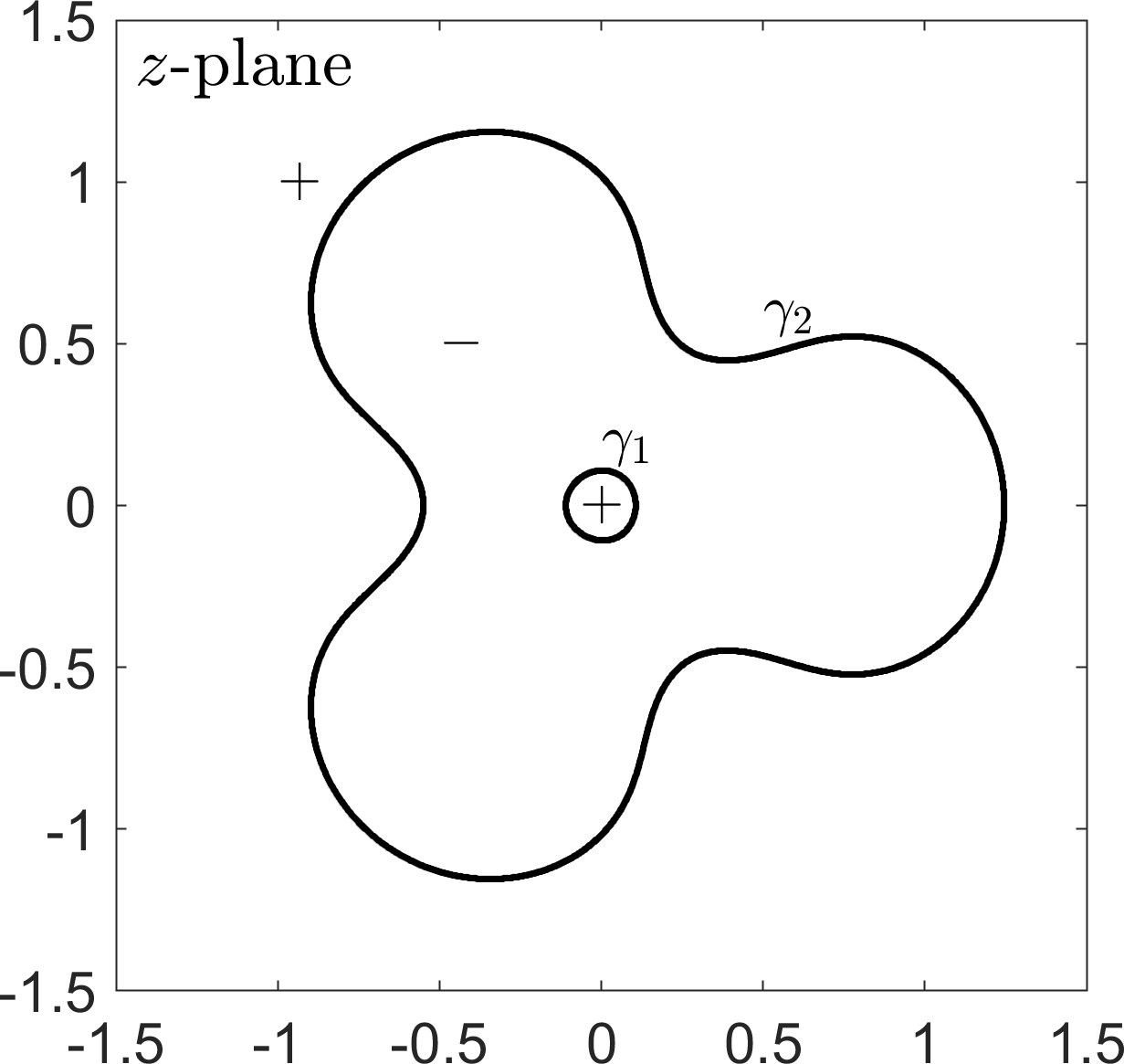
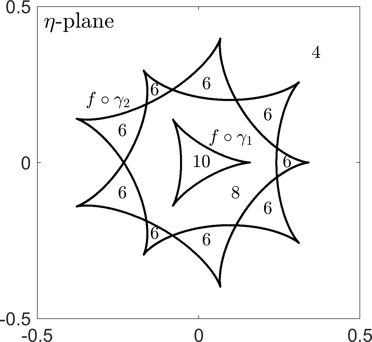
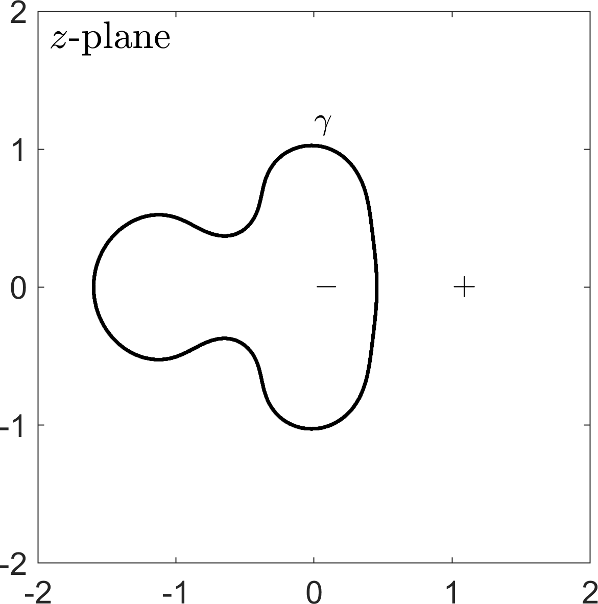
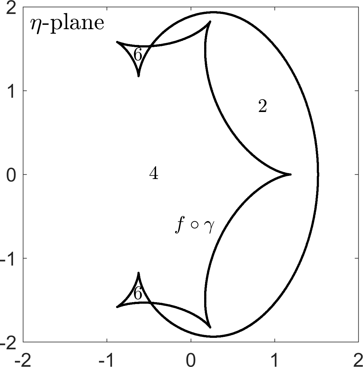
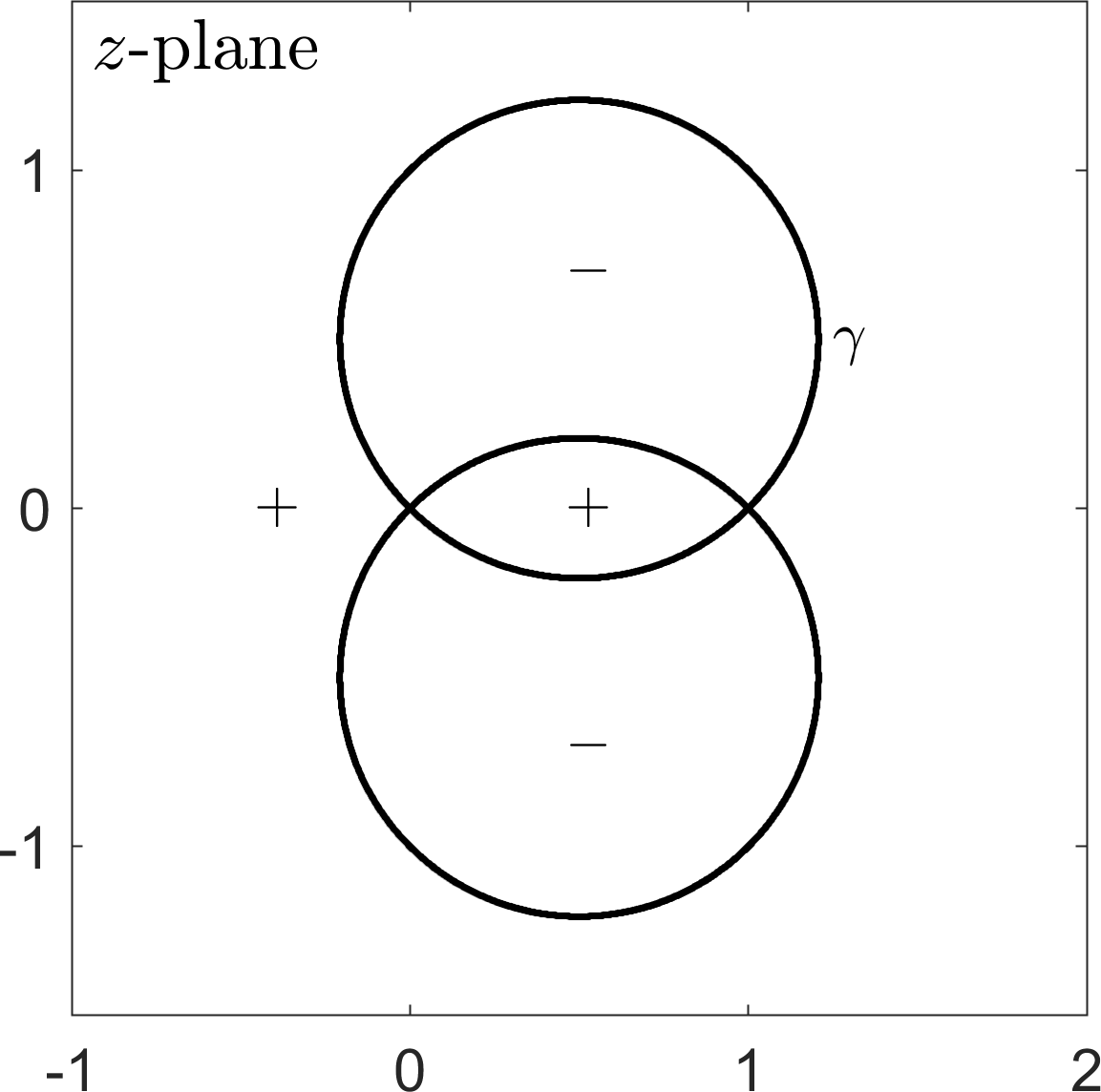
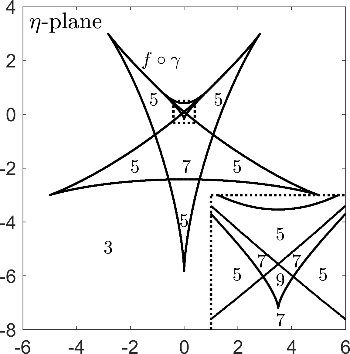
Figure 4: Critical curves (left) and caustics (right) of the functions in Examples 3.9 (top), 3.10 (middle), and 3.11 (bottom). The $+/-$ signs indicate the regions where $f$ is sense-preserving/sense-reversing. The numbers indicate the number of pre-images of an $\eta$ in the respective caustic tile. The dotted line in the bottom right plot marks a zoom-in.

Example 3.9

Consider the non-degenerate rational harmonic mapping

$$f(z)=z-\overline{\left(\frac{z^{2}}{z^{3}-0.6^{3}}\right)}.$$

Figure 4 (top) shows the critical set and the caustics of $f$. We have $P(f)=4$, since $f$ has four simple poles ($\infty$ with index $-1$, the others with index $1$); see Proposition 2.10. Thus, for $\eta$ in the outer region, i.e., with $n(f\circ\gamma_{j};\eta)=0$ for $j=1,2$, we have $N_{\eta}(f)=4+2\cdot 0=4$. For $\eta=0$, we have $n(f\circ\gamma_{1};0)=1$ and $n(f\circ\gamma_{2};0)=2$, so that $f$ has $N_{0}(f)=4+2\cdot 3=10$ zeros.

Certain rational harmonic mappings are studied in gravitational lensing in astrophysics; see e.g. [18, 25]. Also transcendental functions such as $f(z)=z-\overline{k/\sin(z)}$ appear in this context [6].

Example 3.10

Figure 4 (middle) shows the critical curves and caustics of the non-degenerate harmonic mapping

$$f(z)=z^{2}+\frac{1}{\overline{z}}+\frac{1}{\overline{z}+1}+2\log\lvert z\rvert.$$

Here, $P(f)=4$ from the simple poles at $0$ and $-1$ with index $+1$ and the double pole at $\infty$ with index $-2$; see Proposition 2.10. Consequently, any $\eta$ in the outer region (i.e., with $n(f\circ\gamma;\eta)=0$) has $4$ pre-images. Note the effect of deltoid-like, cardioid-like and mixed caustic tiles described above: the tiles where $\eta$ has $6$ pre-images are deltoid-like, the tile where $\eta$ has $2$ pre-images is cardioid-like, and the outer tile is mixed.

Example 3.11

The non-degenerate harmonic polynomial

$$f(z)=p(z)+\overline{q(z)}=z^{n}+(z-1)^{n}+\overline{iz^{n}-i(z-1)^{n}},\quad n\geq 1,$$

has the maximum number of $n^{2}$ zeros [38, p. 2080]. Its critical set consists of $n-1$ circles, intersecting in $0$ and $1$, and can be parametrized as discussed in Section 3.1. Figure 4 (bottom) shows the critical set and caustics for $n=3$.

4 Location of pre-images near the critical set

In Section 3, we omitted the case when $\eta$ is on a caustic. Here, we study the local effect when $\eta$ “crosses” a caustic, i.e., when the number of pre-images changes. Since this is a local effect, the harmonic mappings are neither required to be globally defined nor to be non-degenerate.

Non-singular pre-images persist under a small change of $\eta$, which is an immediate consequence of the inverse function theorem.

Proposition 4.1

Let $f$ be a harmonic mapping defined in the open set $\Omega\subseteq\mathbb{C}$ and let $f$ be non-singular at $z_{0}\in\Omega$. Then there exist open neighborhoods $U\subseteq\Omega\setminus\mathcal{C}$ of $z_{0}$ and $V$ of $f(z_{0})$ such that each $\eta\in V$ has exactly one pre-image under $f$ in $U$.

Lyzzaik [27] investigated the local behavior of light harmonic mappings, defined on an open and simply connected subset of $\mathbb{C}$. His analysis relies upon the local transformation of $f$ near a critical point $z_{0}\in\mathcal{C}$ into standard mappings $h_{2}\circ f\circ h_{1}^{-1}(z)=z^{n}$ or $h_{2}\circ f\circ h_{1}^{-1}(z)=\overline{z}^{n}$, where $h_{1}$ and $h_{2}$ are sense-preserving homeomorphisms; see [27, Sect. 3] for details. If such a standard mapping exists we write $f_{z_{0}}\sim z^{n}$ and $f_{z_{0}}\sim\overline{z}^{n}$ respectively. One of Lyzzaik’s results is the following: Let $f(z_{0})$ be a fold and $U$ be a neighborhood of $z_{0}$. Then there exists a partition $U_{1},U_{2}$ of $U\setminus\mathcal{C}$ with $f_{z_{0}}\sim z$ in $\overline{U}_{1}$ and $f_{z_{0}}\sim\overline{z}$ in $\overline{U}_{2}$. Similarly, if $f(z_{0})$ is a cusp and $h^{\prime}(z_{0})\neq 0$, we have $f_{z_{0}}\sim z^{3}$ in $\overline{U}_{1}$, $f_{z_{0}}\sim\overline{z}$ in $\overline{U}_{2}$ or $f_{z_{0}}\sim z$ in $\overline{U}_{1}$, $f_{z_{0}}\sim\overline{z}^{3}$ in $\overline{U}_{2}$; see [27, Thm. 5.1]. This allows to determine the valence

$$V(f;U)=\sup_{\eta\in\mathbb{C}}\,N_{\eta}(f;U)=\sup_{\eta\in\mathbb{C}}\,\lvert\{z\in U:f(z)=\eta\}\rvert$$

of $f$ in $U$. In particular we have

$$V(f;D_{\varepsilon}(z_{0}))=\begin{cases}2,&\text{if }f(z_{0})\text{ is a fold},\\ 3,&\text{if }f(z_{0})\text{ is a cusp with }h^{\prime}(z_{0})\neq 0,\end{cases}$$ (4.1)

for sufficiently small $\varepsilon>0$; see [27, Thm 5.1]. However, the above transformations are not immediately available for practical computations in general.

We complement Lyzzaik’s work by investigating which values near a fold $\eta=f(z_{0})$ have actually $2$, $1$ or no pre-images under $f$ in $D_{\varepsilon}(z_{0})$, and by approximately locating the pre-images for certain $\eta$. For this we use convergence results on the harmonic Newton iteration

$$z_{k+1}=z_{k}-\frac{\overline{h^{\prime}(z_{k})}f(z_{k})-\overline{g^{\prime}(z_{k})f(z_{k})}}{J_{f}(z_{k})},\quad k\geq 0,$$ (4.2)

from [33]. If the sequence (4.2) converges and all iterates $z_{k}$ are in $D\subseteq\mathbb{C}$, then there exists a zero of $f$ in $\overline{D}$. The proof of the next theorem relies on this strategy.

Theorem 4.2

Let $f$ be a light harmonic mapping and $z_{0}\in\mathcal{C}\setminus\mathcal{M}$, such that $\eta=f(z_{0})$ is a fold. Moreover, let

$$f(z)=\sum_{k=0}^{\infty}a_{k}(z-z_{0})^{k}+\overline{\sum_{k=0}^{\infty}b_{k}(z-z_{0})^{k}}\quad\text{and}\quad c=-\left(\frac{a_{2}\overline{b}_{1}}{a_{1}}+\frac{\overline{b}_{2}a_{1}}{\overline{b}_{1}}\right).$$

Then, for all sufficiently small $\varepsilon>0$, there exists a $\delta>0$, such that for all $0<t<\delta$ we have:

1. $\eta+tc$ has exactly two pre-images under $f$ in $D_{\varepsilon}(z_{0})$,

2. $\eta$ has exactly one pre-image under $f$ in $D_{\varepsilon}(z_{0})$,

3. $\eta-tc$ has no pre-image under $f$ in $D_{\varepsilon}(z_{0})$.

In case 1, each disk $\{z\in\mathbb{C}:\lvert z-z_{\pm}\rvert\leq\text{const}\cdot t\}$, where $z_{\pm}=z_{0}\pm i\sqrt{t\,\overline{b}_{1}/a_{1}}$, contains one of the two pre-images, and $f$ is sense-preserving at one and sense-reversing at the other.

Since $z_{0}\in\mathcal{C}$ and $f(z_{0})$ is a fold, we have $h^{\prime}(z_{0})\neq 0$, and hence $\lvert g^{\prime}(z_{0})\rvert=\lvert h^{\prime}(z_{0})\rvert\neq 0$. Then there exists $\theta\in[0,\pi[$ with $\overline{b}_{1}=a_{1}e^{i2\theta}$, and

$$c=-a_{1}e^{i\theta}\left(\frac{a_{2}}{a_{1}}e^{i\theta}+\overline{\frac{b_{2}}{b_{1}}e^{i\theta}}\right)$$

is non-zero by Lemma 2.4.

1. We apply the harmonic Newton iteration (4.2) to the shifted function $f_{\eta+tc}=f-(\eta+tc)$ with initial points $z_{\pm}$. By [33, Lem. 5.1, Thm. 5.2] and their proofs, the respective sequences of iterates remain in $D_{\pm}$, and converge to two distinct zeros of $f_{\eta+tc}$ for all sufficiently small $t>0$. Thus, $\eta+tc$ has exactly two pre-images under $f$ in $D_{\varepsilon}(z_{0})$, using (4.1).

2. Since $f$ is light and $f(z_{0})=\eta$, there exists $\varepsilon>0$ such that $z_{0}$ is the only pre-image of $\eta$ in $D_{\varepsilon}(z_{0})$.

3. We show first that the “direction” $c$ is not tangential to the caustic, and hence that $\eta+tc$ and $\eta-tc$ are not in the same caustic tile. Since $\eta=f(z_{0})$ is a fold, we have with $z_{0}=\gamma(t_{0})$ and the tangent $\tau$ from Lemma 2.1

$$\overline{\tau(t_{0})}c=-\psi(t_{0})e^{it_{0}/2}a_{1}e^{i\theta}\left(\frac{a_{2}}{a_{1}}e^{i\theta}+\overline{\frac{b_{2}}{b_{1}}e^{i\theta}}\right)=\mp\psi(t_{0})\lvert a_{1}\rvert\left(\frac{a_{2}}{a_{1}}e^{i\theta}+\overline{\frac{b_{2}}{b_{1}}e^{i\theta}}\right),$$

since $e^{it_{0}/2}e^{i\theta}a_{1}=\pm\lvert a_{1}\rvert$; see the proof of Lemma 2.4. Since $\psi$ is real, and non-zero at a fold, we have $\operatorname{Im}(\overline{\tau(t_{0})}c)\neq 0$ by Lemma 2.4. Hence, for a sufficiently small $t>0$, the points $\eta+tc$ and $\eta-tc$ are on different sides of the caustic $f\circ\gamma$, where $\gamma$ denotes the critical curve through $z_{0}$. Thus, there are either $2+2=4$ or $2-2=0$ pre-images of $\eta-tc$ under $f$ in $D_{\varepsilon}(z_{0})$; see Theorem 3.4 if $f$ is non-degenerate, and [28, Thm. 6.7] for light harmonic mappings. Since $V(f;D_{\varepsilon}(z_{0}))=2$ by (4.1), only the latter case is possible.

Moreover, the two pre-images of $\eta+tc$ in 1. lie on different sides of the corresponding critical arc, and hence $f$ is sense-preserving at one pre-image and sense-reversing at the other; see Theorem 3.3 and Remark 3.5 if $f$ is non-degenerate, and again [28, Thm. 6.7] for light harmonic mappings.

Figure 5: Behavior at a fold (top) and cusp (bottom); cf. [21, Figs. 4, 7].

Figure 5 (top) illustrates the effect in Theorem 4.2. The points $z_{1}$, $z_{2}$ are the pre-images of $\eta+tc$ under $f$, i.e., the limits of the harmonic Newton iteration for $f-(\eta+tc)$ with initial points $z_{\pm}$.

Remark 4.3

1. From the proof of Lemma 2.4 we have $\operatorname{Im}(\overline{\tau(t_{0})}c)>0$, i.e., $\tau(t_{0})$ and $c$ form a right-handed ($\mathbb{R}$-)basis. Combining Theorem 4.2 with Proposition 4.1 allows to replace $c$ by any direction $d$ with $\operatorname{Im}(\overline{\tau(t_{0})}d)>0$ without changing the number of pre-images in $D_{\varepsilon}(z_{0})$. More generally, if $\widetilde{\eta}$ is in the same caustic tile as $\eta+tc$ (the tile containing the tangent) and close enough to $\eta$, then $\widetilde{\eta}$ has $2$ pre-images under $f$ in $D_{\varepsilon}(z_{0})$, and similarly in the other cases.

2. For a fold $\eta$ with several pre-images in $\mathcal{C}$, the effect of Theorem 4.2 happens at all points in $f^{-1}(\{\eta\})\cap\mathcal{C}$ simultaneously; see Example 4.4.

3. Theorem 4.2 only covers pre-images in $D_{\varepsilon}(z_{0})$. All other non-singular pre-images of $\eta$ under $f$ persist by Proposition 4.1, when going from $\eta$ to $\eta\pm tc$, provided that $t>0$ is sufficiently small.

When $\eta$ is a cusp as in (4.1), we have a similar result, which is also based on the harmonic Newton iteration; see [33, Thm. 5.2, 2.]. For $\widetilde{\eta}$ close enough to $\eta$ on one side of the caustic, there are $3$ pre-images by [27, Thm 5.1], and on the other side there is only $1$ pre-image by Proposition 4.1 and Theorem 4.2; see Figure 5 (bottom).

The next example illustrates the local behavior near critical points corresponding to a fold, a cusp, and a double fold, and near a point in $\mathcal{M}$.

Example 4.4

We consider the harmonic mapping $f(z)=\frac{1}{3}z^{3}+\frac{1}{2}\overline{z}^{2}$, which is similar to the one in [28, Ex. 5.17]. Since $J_{f}(z)=\lvert z\rvert^{2}-\lvert z\rvert^{4}$, we have $\mathcal{C}=\partial\mathbb{D}\cup\{0\}$ and $\mathcal{M}=\{0\}$. The caustics of $f$ are shown in Figure 6, together with certain points $\eta_{1},\ldots,\eta_{6}$. While “moving” $\eta$ from $\eta_{1}=-0.4$ to $\eta_{6}=0.9$ we reach a double fold, a point in $f(\mathcal{M})$, a fold and a cusp. The respective pre-images of $\eta_{j}$ under $f$ are shown in Figure 7, and have been computed with the harmonic Newton method [33]. The background is colored according to the phase $f_{\eta_{j}}/\lvert f_{\eta_{j}}\rvert$ of the shifted function $f_{\eta_{j}}=f-\eta_{j}$; see [37] for an extensive discussion of phase plots. The Poincaré index of $f$ at $z_{0}$ corresponds to the color change on a small circle around $z_{0}$ in the positive direction. In particular, we have $\operatorname{ind}(f_{\eta_{j}};z_{0})=+1$ for zeros $z_{0}$ in $\mathbb{C}\setminus\overline{\mathbb{D}}$, and $\operatorname{ind}(f_{\eta_{j}};z_{0})=-1$ for zeros $z_{0}$ in $\mathbb{D}\setminus\{0\}$; see also Proposition 2.7. A feature is the zero $0\in\mathcal{M}$ of $f$, for which $\operatorname{ind}(f;0)=-2$ by (2.13). This reflects the fact that two pre-images where $f$ is sense-reversing merge together at $0$; see Remark 2.8.

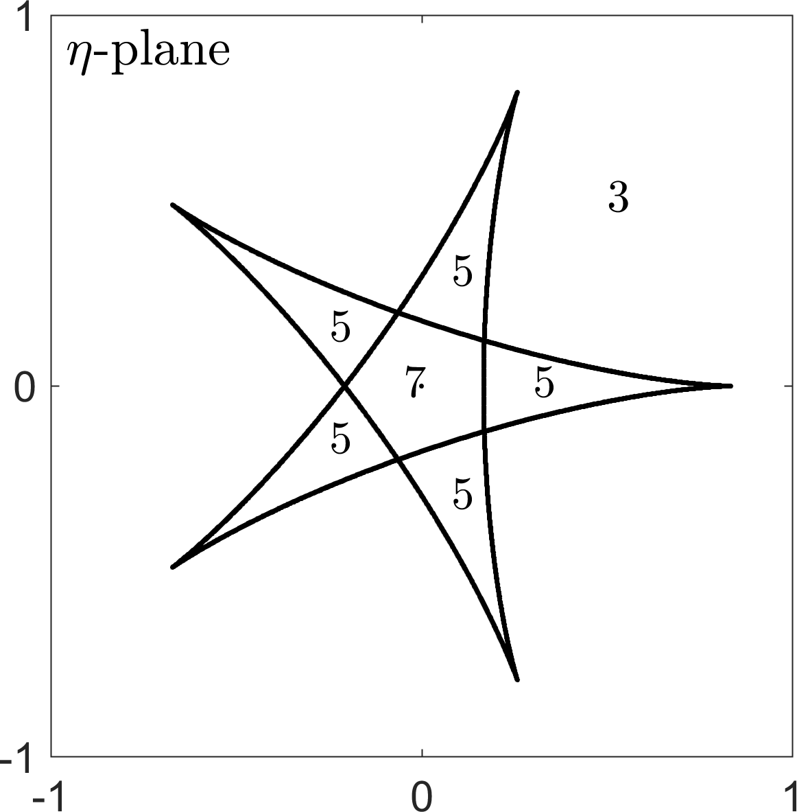
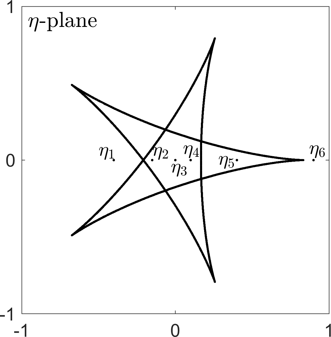
Figure 6: Caustics of $f(z)=\frac{1}{3}z^{3}+\frac{1}{2}\overline{z}^{2}$; see Example 4.4.

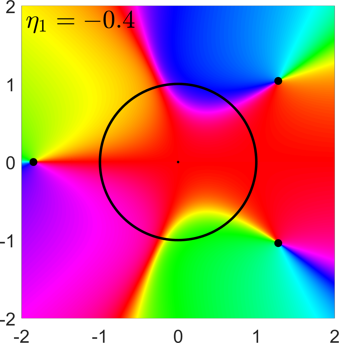
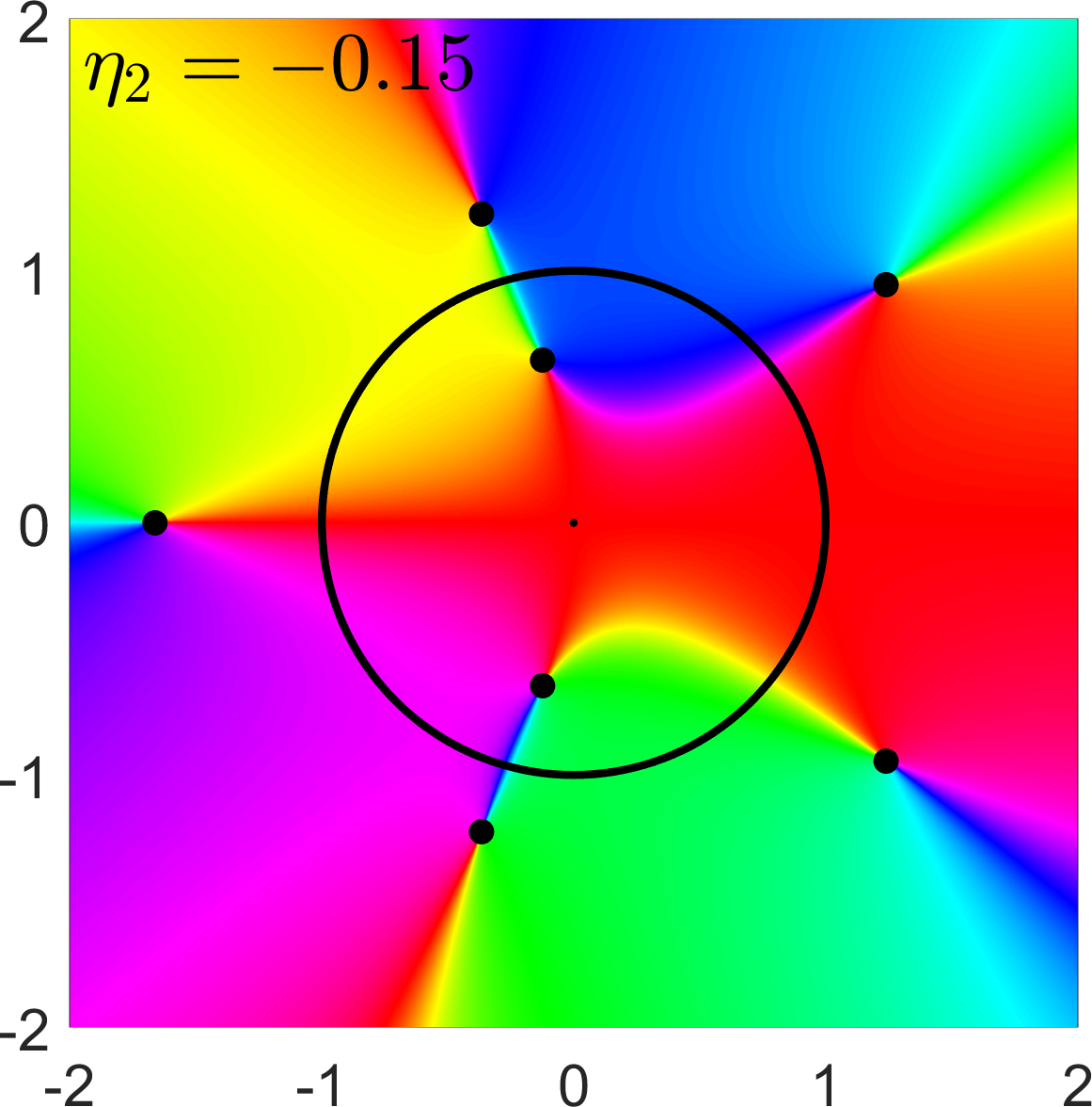
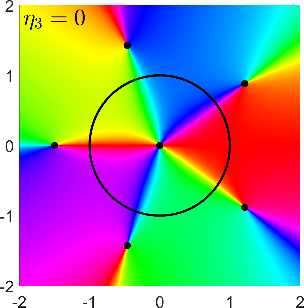
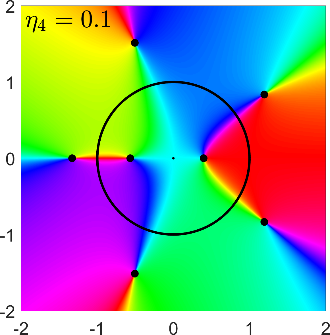
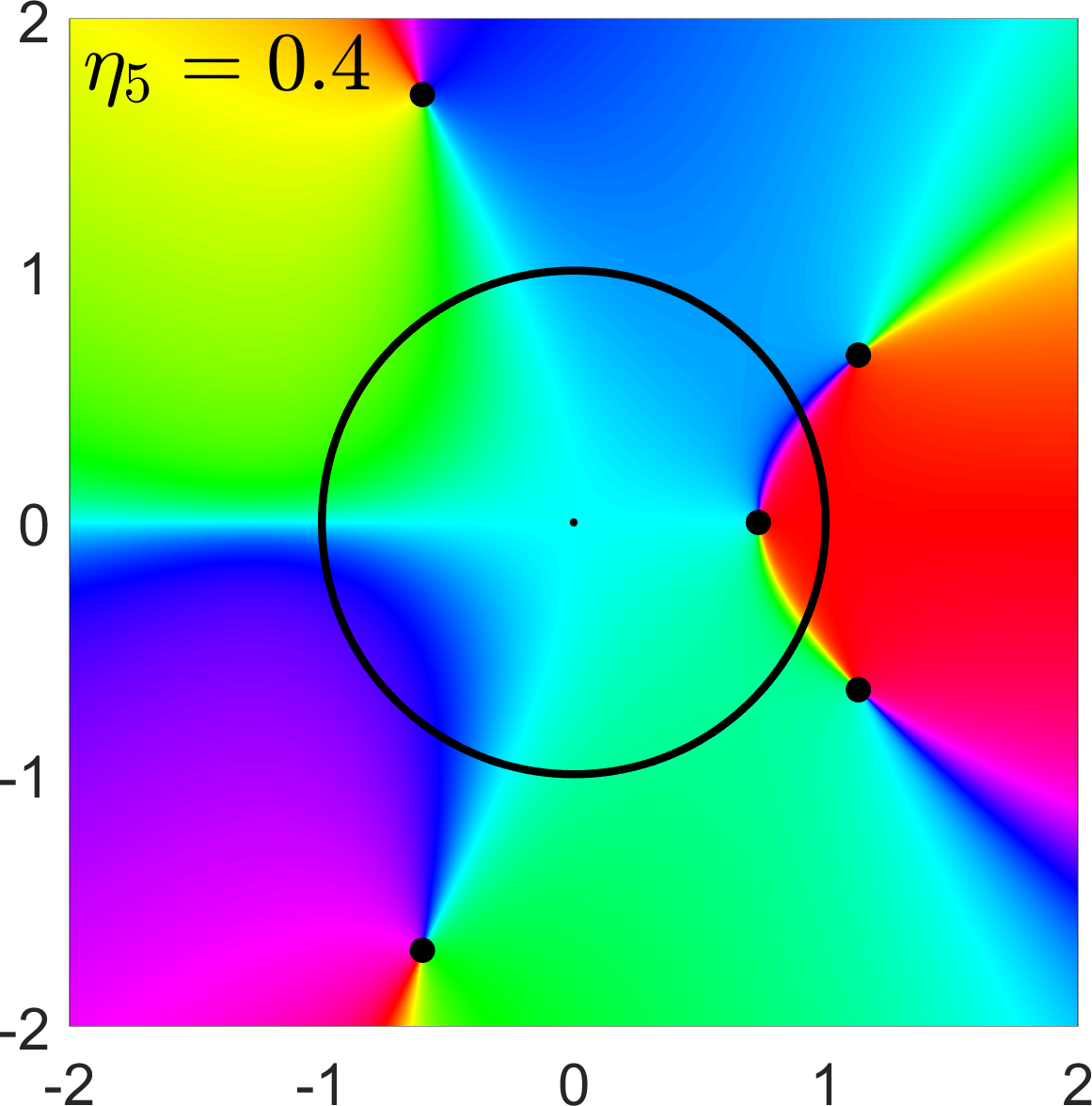
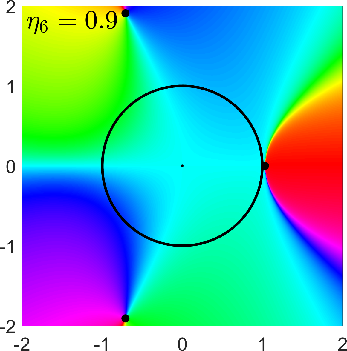
Figure 7: Phase plots of $f_{\eta_{j}}(z)=\frac{1}{3}z^{3}+\frac{1}{2}\overline{z}^{2}-\eta_{j}$ (see Figure 6). Black dots indicate zeros of $f_{\eta_{j}}$. The critical set $\mathcal{C}=\partial\mathbb{D}\cup\{0\}$ is displayed in black.

5 On the number of zeros of harmonic polynomials

We consider harmonic polynomials

$$f(z)=p(z)+\overline{q(z)}=\sum_{k=0}^{n}a_{k}z^{k}+\overline{\sum_{k=0}^{m}b_{k}z^{k}},\quad n\geq m,$$ (5.1)

with $a_{n}\neq 0\neq b_{m}$. These are non-degenerate if and only if $\lvert a_{n}\rvert\neq\lvert b_{n}\rvert$, where we define $b_{n}=0$ for $n>m$. Such functions have at most $n^{2}$ zeros and this bound is sharp [38]. By the argument principle, $f$ has at least $n$ zeros, if none of them is singular. If $f$ has fewer than $n$ zeros, at least one has to be in $\mathcal{M}$. However, counting the zeros with their Poincaré indices as multiplicities gives again at least $n$ zeros in total.

For $n>m\geq 1$, we study the maximum valence of harmonic polynomials

$$V_{n,m}=\max\{N(p(z)+\overline{q(z)}):\deg(p)=n,\deg(q)=m\},$$

where $N(f)$ denotes the number of zeros of $f$. We have $V_{n,m}\leq n^{2}$ from [38], but the quantity $V_{n,m}$ is only known in special cases, namely $V_{n,1}=3n-2$ from [19, 13] and $V_{n,n-1}=n^{2}$ from [38]. We show in this section, that for given $n>m\geq 1$ and every $k\in\{n,n+1,\ldots,V_{n,m}\}$, there exists a harmonic polynomial (5.1) with $k$ zeros, i.e., every number of zeros between the lower and upper bound occurs. This generalizes [7, Thm. 1.1]. More precisely, we can achieve all these numbers by just changing $a_{0}$, which is equivalent to considering the pre-images of a certain $\eta$ instead of the zeros.

If $\eta$ crosses a single caustic arc at a fold, the number of pre-images changes by $\pm 1$ ($\eta$ on the caustic) and $\pm 2$ ($\eta$ on the “other side” of the caustic) by Theorems 3.7 and 4.2. The key difficulty now is to handle multiple caustic arcs, i.e., caustic arcs which are the image of several different critical arcs.

Example 5.1

Consider $f(z)=\frac{1}{2}p(z)^{2}+\overline{p(z)}$ with $p(z)=z^{2}-1$. Then $J_{f}(z)=\lvert p^{\prime}(z)\rvert^{2}(\lvert p(z)\rvert^{2}-1)$, and $\mathcal{C}=\{z\in\mathbb{C}:\lvert p(z)\rvert=1\}$ consists of the two curves $\gamma_{\pm}(t)=\pm\sqrt{1+e^{it}}$, $-\pi\leq t\leq\pi$. Since $p(\gamma_{+}(t))=p(\gamma_{-}(t))$, the harmonic mapping $f$ maps $\gamma_{\pm}$ onto the same caustic.

More generally, let $\gamma$ be a closed curve with $\lvert g^{\prime}(w)/h^{\prime}(w)\rvert=1$ on $\operatorname{trace}(\gamma)$, and let $w=p(z)$ such that $\operatorname{trace}(\gamma)$ has $k\geq 2$ disjoint pre-images under $p$. Then these pre-images are in the critical set of $f(z)=h(p(z))+\overline{g(p(z))}$ and are mapped to the same caustic. In particular, $h(z)=\frac{1}{n}z^{n}$, $g(z)=\frac{1}{m}z^{m}$ with $n>m\geq 1$ provides an example of a non-degenerate harmonic polynomial with $k$ critical curves that are mapped onto the same caustic.

Multiple caustic arcs can be eliminated by a polynomial perturbation of $f$. We write $\mathcal{C}_{f}$ and $\mathcal{C}_{F}$ for the critical sets of $f$ and $F$, respectively.

Lemma 5.2

Let $f$ be a harmonic mapping, and $z_{1},z_{2}\in\mathcal{C}_{f}$, $z_{1}\neq z_{2}$, with $f(z_{1})=f(z_{2})$. Then there exists a polynomial $p$ with $\deg(p)=3$, such that $z_{1},z_{2}\in\mathcal{C}_{F}$ for $F=f+p$, but $F(z_{1})\neq F(z_{2})$.

Let $\varepsilon>0$, and let $p$ be the (unique) Hermite interpolation polynomial of degree $3$ with $p(z_{1})=\varepsilon$, $p(z_{2})=-\varepsilon$, and $p^{\prime}(z_{1})=0=p^{\prime}(z_{2})$. We then have $J_{F}(z_{1})=0=J_{f}(z_{1})$, and the same for $z_{2}$, but $F(z_{1})\neq F(z_{2})$.

Next, we show that sufficiently small perturbations do not decrease the number of non-singular zeros.

Lemma 5.3

Let $f$ and $g$ be harmonic mappings, such that $f$ has only finitely many zeros, which are all non-singular, and such that $g$ has no singularities at the zeros of $f$. Then $N(f)\leq N(f+\varepsilon g)$ for all sufficiently small $\varepsilon>0$.

Let $z_{1},\dots,z_{n}$ be the zeros of $f$. Since non-singular zeros are isolated [12, p. 413], there exists $\delta>0$, such that $D_{\delta}(z_{j})\cap\mathcal{C}=\varnothing$, $f$ and $g$ have no other exceptional points than $z_{j}$ in $\overline{D_{\delta}(z_{j})}$ for $j=1,\dots,n$, and $D_{\delta}(z_{j})\cap D_{\delta}(z_{k})=\varnothing$ for $j\neq k$.

Define $\Gamma=\cup_{k=1}^{n}\partial D_{\delta}(z_{k})$ and let $\varepsilon>0$ such that

$$\varepsilon\cdot\max\{\lvert g(z)\rvert:z\in\Gamma\}<\min\{\lvert f(z)\rvert:z\in\Gamma\}.$$

Then we have for $z\in\Gamma$

$$\lvert f(z)-(f(z)+\varepsilon g(z))\rvert=\varepsilon\lvert g(z)\rvert<\lvert f(z)\rvert.$$

By Rouché’s theorem (e.g. [32, Thm. 2.3]) and the argument principle applied on each $\partial D_{\delta}(z_{k})$, we get

$$N(f)=\sum_{k=1}^{n}N(f;D_{\delta}(z_{k}))\leq\sum_{k=1}^{n}N(f+\varepsilon g;D_{\delta}(z_{k}))\leq N(f+\varepsilon g),$$

which settles the proof.

With the Lemmas 5.2 and 5.3 we get the following result on the possible number of zeros of harmonic polynomials.

Theorem 5.4

Let $n>m\geq 1$ and $k\in\{n,n+1,\ldots,V_{n,m}\}$. Then there exists a harmonic polynomial $f(z)=p(z)+\overline{q(z)}$ with $\deg(p)=n$ and $\deg(q)=m$, and with $k$ zeros.

Moreover, if $k$ and $n$ have different parity ($n-k$ is odd), then $f$ is singular, i.e., $0$ is a caustic point of $f$. If $k$ and $n$ have the same parity, then there exists a non-singular $f$, as prescribed above.

Let $f(z)=p(z)+\overline{q(z)}$ be a harmonic polynomial with $\deg(p)=n$, $\deg(q)=m$, and with $V_{n,m}$ zeros, which exists by the definition of $V_{n,m}$. Without loss of generality, we can assume that $f$ has no multiple caustic arcs. Indeed, when $n=2$ the only critical curve of $f$ is the image of the unit circle under a Möbius transformation, and hence there are no multiple caustic arcs. If $n\geq 3$ and if $f$ has multiple caustic arcs we resolve them by Lemma 5.2 with a polynomial perturbation of degree $3$, such that no other multiple caustic arcs occur. For sufficiently small $\varepsilon>0$, the resulting harmonic polynomial has at most $V_{n,m}$ zeros, and at least $V_{n,m}$ zeros by Lemma 5.3. This gives a harmonic polynomial with $V_{n,m}$ zeros and without multiple caustic arcs.

By Theorem 3.6, there exists an $\eta_{n}\in\mathbb{C}$ with $N_{\eta_{n}}(f)=n$. Let $\phi$ be a curve from $\eta_{n}$ to $0$, which intersects the caustics only in folds corresponding to a single caustic arc. Such a curve exists since (possible) multiple caustic arcs are already resolved, and since the zeros of $\psi$ are isolated by Lemma 2.1. Note that $f$ is light since any $f-\eta$ has at most $n^{2}$ zeros. Then by Theorems 3.7 and 4.2, all $k=n,n+1,\ldots,V_{n,m}$ appear as number of pre-images under $f$ for an appropriate $\eta_{k}\in\operatorname{trace}(\phi)$, i.e., $N_{\eta_{k}}(f)=k$, and hence $f-\eta_{k}$ is a harmonic polynomial with $k$ zeros.

The second part follows from Theorem 3.7 and the fact that $\eta_{n}$ can be chosen in $\mathbb{C}\setminus f(\mathcal{C})$; see Theorem 3.6.

Remark 5.5

Let $n>m\geq 1$. By the proof of Theorem 5.4, there exists a harmonic polynomial $f(z)=p(z)+\overline{q(z)}$ with $\deg(p)=n$, $\deg(q)=m$, and $\eta_{n},\ldots$, $\eta_{V_{n,m}}\in\mathbb{C}$, such that $f-\eta_{k}$ has $k$ zeros. Moreover, $\eta_{n+1},\eta_{n+3},\ldots$ are on the caustics of $f$, and $\eta_{n},\eta_{n+2},\ldots$ can be chosen in caustic tiles.

Since $V_{n,n-1}=n^{2}$, we have the following corollary.

Corollary 5.6

Let $n\geq 2$. For each $k\in\{n,n+1,\ldots,n^{2}\}$, there exists a harmonic polynomial as in (5.1) with $k$ zeros.

6 Outlook

A further study of the geometry of the caustics should be of interest, e.g., the number of cusps. This an important open problem posed by Petters [29, p. 1399] for certain harmonic mappings from gravitational lensing.

While we considered harmonic mappings on the Riemann sphere (minus possible poles) in this work, also harmonic mappings in bounded domains (similar to [28]) and on more general Riemann surfaces might be of interest. We expect similar results for these domains of definition.

The results in Section 5 could probably be generalized to a broader class of harmonic mappings, e.g., non-degenerate rational harmonic mappings $f(z)=r(z)+\overline{s(z)}$, using the same approach as above. However, one would have to handle multiple caustic arcs in a different way.

Acknowledgments.

We thank Jörg Liesen for several helpful comments on the manuscript. Moreover, we are grateful to the anonymous referees for many valuable comments, which lead to improvements of this work.

References

- [1] L. V. Ahlfors, Lectures on quasiconformal mappings, D. Van Nostrand Co., Inc., Toronto, Ont.-New York-London, 1966.
- [2] J. H. An and N. W. Evans, The Chang–Refsdal lens revisited, Monthly Notices Roy. Astronom. Soc., 369 (2006), pp. 317–334.
- [3] M. B. Balk, Polyanalytic Functions, vol. 63 of Mathematical Research, Akademie-Verlag, Berlin, 1991.
- [4] A. F. Beardon, Complex analysis. The argument principle in analysis and topology, John Wiley & Sons, Ltd., Chichester, 1979.
- [5] C. Bénéteau and N. Hudson, A survey on the maximal number of solutions of equations related to gravitational lensing, in Complex analysis and dynamical systems, Trends Math., Birkhäuser/Springer, Cham, 2018, pp. 23–38.
- [6] W. Bergweiler and A. Eremenko, On the number of solutions of a transcendental equation arising in the theory of gravitational lensing, Comput. Methods Funct. Theory, 10 (2010), pp. 303–324.
- [7] P. M. Bleher, Y. Homma, L. L. Ji, and R. K. W. Roeder, Counting zeros of harmonic rational functions and its application to gravitational lensing, Int. Math. Res. Not. IMRN, (2014), pp. 2245–2264.
- [8] B. Bollobás, Modern graph theory, vol. 184 of Graduate Texts in Mathematics, Springer-Verlag, New York, 1998.
- [9] D. Bshouty and A. Lyzzaik, Problems and conjectures in planar harmonic mappings, J. Anal., 18 (2010), pp. 69–81.
- [10] J. Clunie and T. Sheil-Small, Harmonic univalent functions, Ann. Acad. Sci. Fenn. Ser. A I Math., 9 (1984), pp. 3–25.
- [11] P. Duren, Harmonic mappings in the plane, vol. 156 of Cambridge Tracts in Mathematics, Cambridge University Press, Cambridge, 2004.
- [12] P. Duren, W. Hengartner, and R. S. Laugesen, The argument principle for harmonic functions, Amer. Math. Monthly, 103 (1996), pp. 411–415.
- [13] L. Geyer, Sharp bounds for the valence of certain harmonic polynomials, Proc. Amer. Math. Soc., 136 (2008), pp. 549–555.
- [14] W. Hengartner and G. Schober, Univalent harmonic functions, Trans. Amer. Math. Soc., 299 (1987), pp. 1–31.
- [15] P. Henrici, Applied and computational complex analysis. Vol. 3, Pure and Applied Mathematics (New York), John Wiley & Sons, Inc., New York, 1986.
- [16] D. Khavinson, S.-Y. Lee, and A. Saez, Zeros of harmonic polynomials, critical lemniscates, and caustics, Complex Anal. Synerg., 4 (2018), p. 4:2.
- [17] D. Khavinson and G. Neumann, On the number of zeros of certain rational harmonic functions, Proc. Amer. Math. Soc., 134 (2006), pp. 1077–1085.
- [18] D. Khavinson and G. Neumann, From the fundamental theorem of algebra to astrophysics: a “harmonious” path, Notices Amer. Math. Soc., 55 (2008), pp. 666–675.
- [19] D. Khavinson and G. Świa̧tek, On the number of zeros of certain harmonic polynomials, Proc. Amer. Math. Soc., 131 (2003), pp. 409–414.
- [20] S.-Y. Lee, A. Lerario, and E. Lundberg, Remarks on Wilmshurst’s theorem, Indiana Univ. Math. J., 64 (2015), pp. 1153–1167.
- [21] J. Liesen and J. Zur, How constant shifts affect the zeros of certain rational harmonic functions, Comput. Methods Funct. Theory, 18 (2018), pp. 583–607.
- [22] J. Liesen and J. Zur, The maximum number of zeros of revisited, Comput. Methods Funct. Theory, 18 (2018), pp. 463–472.
- [23] N. G. Lloyd, Degree theory, Cambridge University Press, Cambridge-New York-Melbourne, 1978. Cambridge Tracts in Mathematics, No. 73.
- [24] R. Luce and O. Sète, The index of singular zeros of harmonic mappings of anti-analytic degree one, Complex Var. Elliptic Equ., (2019), pp. 1–21.
- [25] R. Luce, O. Sète, and J. Liesen, Sharp parameter bounds for certain maximal point lenses, Gen. Relativity Gravitation, 46 (2014), pp. 1–16.
- [26] R. Luce, O. Sète, and J. Liesen, A note on the maximum number of zeros of , Comput. Methods Funct. Theory, 15 (2015), pp. 439–448.
- [27] A. Lyzzaik, Local properties of light harmonic mappings, Canad. J. Math., 44 (1992), pp. 135–153.
- [28] G. Neumann, Valence of complex-valued planar harmonic functions, Trans. Amer. Math. Soc., 357 (2005), pp. 3133–3167.
- [29] A. O. Petters, Gravity’s action on light, Notices Amer. Math. Soc., 57 (2010), pp. 1392–1409.
- [30] A. O. Petters, H. Levine, and J. Wambsganss, Singularity Theory and Gravitational Lensing, vol. 21 of Progress in Mathematical Physics, Birkhäuser Boston, Inc., Boston, MA, 2001.
- [31] J. Roe, Winding around. The winding number in topology, geometry, and analysis, vol. 76 of Student Mathematical Library, American Mathematical Society, Providence, RI; Mathematics Advanced Study Semesters, University Park, PA, 2015.
- [32] O. Sète, R. Luce, and J. Liesen, Perturbing rational harmonic functions by poles, Comput. Methods Funct. Theory, 15 (2015), pp. 9–35.
- [33] O. Sète and J. Zur, A Newton method for harmonic mappings in the plane, IMA J. Numer. Anal., 40 (2020), pp. 2777–2801.
- [34] T. Sheil-Small, Complex Polynomials, vol. 75 of Cambridge Studies in Advanced Mathematics, Cambridge University Press, Cambridge, 2002.
- [35] T. J. Suffridge and J. W. Thompson, Local behavior of harmonic mappings, Complex Variables Theory Appl., 41 (2000), pp. 63–80.
- [36] J. L. Walsh, The Location of Critical Points of Analytic and Harmonic Functions, American Mathematical Society Colloquium Publications, Vol. 34, American Mathematical Society, New York, N. Y., 1950.
- [37] E. Wegert, Visual complex functions. An introduction with phase portraits., Birkhäuser/Springer Basel AG, Basel, 2012.
- [38] A. S. Wilmshurst, The valence of harmonic polynomials, Proc. Amer. Math. Soc., 126 (1998), pp. 2077–2081.