Automated Fitting of Neural Network Potentials at Coupled Cluster Accuracy: Protonated Water Clusters as Testing Ground

Abstract

Highly accurate potential energy surfaces are of key interest for the detailed understanding and predictive modeling of chemical systems. In recent years, several new types of force fields, which are based on machine learning algorithms and fitted to ab initio reference calculations, have been introduced to meet this requirement. Here we show how high–dimensional neural network potentials can be employed to automatically generate the potential energy surface of finite sized clusters at coupled cluster accuracy, namely CCSD(T*)-F12a/aug-cc-pVTZ. The developed automated procedure utilizes the established intrinsic properties of the model such that the configurations for the training set are selected in an unbiased and efficient way to minimize the computational effort of expensive reference calculations. These ideas are applied to protonated water clusters from the hydronium cation, H3O+, up to the tetramer, H9O4+, and lead to a single potential energy surface that describes all these systems at essentially converged coupled cluster accuracy with a fitting error of 0.06 kJ/mol per atom. The fit is validated in detail for all clusters up to the tetramer and yields reliable results not only for stationary points, but also for reaction pathways, intermediate configurations, as well as different sampling techniques. Per design the NNPs constructed in this fashion can handle very different conditions including the quantum nature of the nuclei and enhanced sampling techniques covering very low as well as high temperatures. This enables fast and exhaustive exploration of the targeted protonated water clusters with essentially converged interactions. In addition, the automated process will allow one to tackle finite systems much beyond the present case.

I Introduction

The potential energy surface (PES) of a system, which governs all its structural, dynamic and thermodynamic properties in the Born–Oppenheimer approximation, is currently in many cases best described by coupled cluster theory, granting the CCDS(T) approach the title of the “gold standard” in quantum chemistry Bartlett and Musiał (2007); Hobza (2012). Thus, it is desirable to utilize this method not only in the realm of static single–point calculations, but also for finite temperature dynamical simulations in order to reach chemical accuracy and provide predictive answers purely based on simulations. However, the excellent quality comes at a rather high price in terms of the computational cost that, moreover, scales very unfavorably with the system size. Advanced simulations, such as rare event sampling techniques or path integral methods, that typically require many million evaluations of the interactions to reach convergence are, therefore, usually out of scope if energies and forces need to be evaluated “on–the–fly” Marx and Hutter (2009) during the simulation. This is the very reason why only notable exceptions exist Spura, Elgabarty, and Kühne (2015); Mouhat et al. (2017); Haycraft, Li, and Iyengar (2017) where correlated electronic structure methods such as coupled cluster theory have been applied on–the–fly to small molecules such as the Zundel cation, H5O2+.

Especially for the study of water, different approaches based on physically motivated functional forms have been very successful in reaching high accuracy as for example shown for the MB-Pol water force field Babin, Leforestier, and Paesani (2013) or other highly accurate fitting schemes Bukowski et al. (2007); Wang et al. (2009); Babin, Medders, and Paesani (2012); see e.g. Ref. 11 for more examples. Being usually based on many–body expansions, such approaches were also recently applied to protonated water clusters, explicitly including up to four body terms Heindel et al. (2018), and shown to reproduce coupled cluster reference calculations with rather high accuracy for stationary point structures. Other notable potentials for protonated water (clusters) rely on empirical models Kozack and Jordan (1992), perturbation theory Hodges and Stone (1999), or are based on empirical valence bond models with increasing complexity of the reference states Lobaugh and Voth (1996); Schmitt and Voth (1998); Vuilleumier and Borgis (1998); James and Wales (2005); Brancato and Tuckerman (2005); Wu et al. (2008); Kumar, Christie, and Jordan (2009).

At the same time, prominent advances in machine learning techniques have led to the development of computationally very efficient, yet accurate potential energy surfaces Handley and Popelier (2010); Behler (2011a, 2016); Bartók et al. (2017); Butler et al. (2018), where various different techniques have been introduced over the years Blank et al. (1995); Prudente, Acioli, and Neto (1998); Lorenz, Groß, and Scheffler (2004); Lorenz, Scheffler, and Gross (2006); Manzhos et al. (2006); Behler and Parrinello (2007); Bartók et al. (2010); Rupp et al. (2012); Shapeev (2015); Li, Kermode, and De Vita (2015); Thompson et al. (2015); Schütt et al. (2017); Chmiela et al. (2017); Faraji et al. (2017); Unke and Meuwly (2019). These methods do not utilize physically motivated functional forms, but rather use highly flexible general functions being able to represent in principle arbitrary functional relations. They are usually trained to electronic structure reference data and can afterwards reproduce the structure–energy relation with high precision. The first such technique, which is scalable to essentially arbitrary system sizes and based on artificial neural networks, is the high–dimensional neural network potential (NNP) methodology Behler and Parrinello (2007); Behler (2017) that has been proven to be well suited for the description of a variety of systems as summarized in Ref. 42. In addition, the high flexibility of the underlying functional relation provides a very powerful tool for the identification of deficiencies in the training set, as first mentioned in Ref. 23 and used in Ref. 43. By comparison of two distinct machine learning potentials which feature large differences for configurations not sufficiently represented, the training set can be iteratively optimized Artrith and Behler (2012). This has enabled the development of iterative strategies for the assembling of the training set for NNPs for example using the notion of adaptive sampling Gastegger, Behler, and Marquetand (2017). In addition, similar strategies were recently also applied to other machine learning approaches in the context of Gaussian approximation potentials Bartók et al. (2010) called data driven learning Deringer, Pickard, and Csányi (2018), or for moment tensor potentials Shapeev (2015) called active learning Podryabinkin and Shapeev (2017). While most of these machine learning approaches have been targeting DFT (density functional theory) reference calculations, recent studies employing machine learning potentials were able to closely reproduce coupled cluster accuracies for finite sized molecular clusters Schran et al. (2018); Schran, Brieuc, and Marx (2018); Chmiela et al. (2018); Smith et al. (2019).

In the following, we will present how high–dimensional neural network potentials can be utilized for the automated fitting of highly–accurate potential energy surfaces to reach coupled cluster accuracy. In the present study, protonated water clusters from the monomer up to the tetramer are chosen as a case study for which converged coupled cluster reference calculations are still feasible. The NNP methodology has already been successfully applied to these clusters using a density functional theory based description for the reference calculations Natarajan, Morawietz, and Behler (2015). In the present work, rather similar fitting accuracies are reached, but the machine learning methodology is used to reproduce much more accurate so–called CCSD(T*)-F12a/aug-cc-pVTZ energies, which provide essentially converged coupled cluster data as described in the computational details. As mentioned above, it is important to note that for molecular systems such as water for instance, very accurate alternative approaches making use of N-body expansions have also been proposed. Examples are as diverse as permutationally invariant polynomials (PIPs) Braams and Bowman (2009), the MB-pol water potential Babin, Leforestier, and Paesani (2013) and also machine learning potentials incorporating low-order many-body terms Bartók et al. (2013). These and related approaches offer the advantage that they are likely to have a better transferability and extrapolation performance for larger systems beyond those that have been explicitly covered by the underlying training set. On the other hand, advantages of our approach are its very general applicability to many different types of systems also beyond those consisting of fixed molecular entities, such as metal clusters Artrith and Behler (2012), the global permutation invariance of all chemically equivalent atoms in arbitrarily large systems, and the resulting unconstrained reactivity as required for instance to describe long-range proton transport processes in bulk systems, which has been demonstrated already for aqueous electolytes like bulk NaOH(aq) Hellström and Behler (2016) as well as for water dissociating at zinc oxide surfaces Quaranta, Hellström, and Behler (2017).

The remaining manuscript is structured as follows: First, the automated fitting procedure for neural network potentials is reviewed in detail. Afterwards, the quality of the resulting potential energy surface is validated with respect to the coupled cluster reference not only for stationary–point structures, but also for reaction pathways and intermediate configurations. Finally, the performance of the NNP for molecular dynamics and path integral simulations is verified explicitly.

II Automated Fitting Procedure for Neural Network Potentials

Application of neural networks to chemically complex systems can be achieved, as reviewed in detail in Ref. 42, by the construction of a structure–energy relation via a transformation of the structure by atom–centered so–called symmetry functions that provide the input for atomic neural networks. These neural networks output atomic energy contributions for all atoms in the system that sum up to the total energy. The resulting functional relation, as schematically depicted in Fig. 1 for the Zundel cation H5O2+, can be analytically differentiated to provide the forces of the system. For further details on atom–centered symmetry functions and the high–dimensional neural network approach we refer the reader to Refs. 56 and 42, respectively, as well as to the supporting information where our particular approach is explained in depth. and recall only that the resulting NNPs are also permutationally invariant.

For the purpose of this study, it is sufficient to stress that this approach provides a highly flexible functional form that can be fitted to a training set with configurations for which the corresponding energies are known. This fit can, afterwards, be used for accurate interpolation between the training points, while extrapolation outside of the configuration space spanned by the training set usually becomes unreliable due to the absence of physically motivated functional forms.

Figure 1: Representation of the structure–energy relation in a high–dimensional neural network potential (NNP) for the specific example of a Zundel cation H5O2+. In a first step, the structure is transformed via atom–centered symmetry functions into rotationally and translationally invariant vectors each of which is represented by a small box $G$. These serve as the input for atomic neural networks to provide atomic energies that sum up to the total energy of the system. This functional relation is analytically differentiable and, thus, can provide the forces of the system.

A key task in the development of neural network potentials is, therefore, the preparation of the reference set used for the training of the potential. It needs to be representative for all envisaged conditions and must sample the spanned configuration space in a balanced manner.

The intrinsic properties of the neural network approach provide a very powerful tool for this difficult task, as first introduced in Ref. 23 and used in Ref. 43. The high flexibility of the functional form results usually in large differences for regions in configuration space that are underrepresented in the training set. Using this approach, unnecessarily large numbers of reference calculations can be avoided, since the calculations can be restricted to the important configurations really needed for an improvement of the potential only where actually required. We note in passing that this strategy is well known in the field of active learning as the “query by committe” approach Seung, Opper, and Sompolinsky (1992). In addition, it has been proven to feature an error that decreases exponentially with the number of training points which already holds for the smallest two-member committee Seung, Opper, and Sompolinsky (1992) that we use here. A second strategy to identify configurations for an improvement of the training set relies on the identification of configurations beyond the boundaries of the configuration space spanned by the training set. Such points are likely to show extrapolation errors and can be identified by comparing the description of the structure encoded in the symmetry function values to the range of the symmetry function values encountered in the training set. Methods to select the most important configurations for an improvement of the training set are especially important if high–level and thus demanding quantum chemistry methods such as CCSD(T) theory shall be used. It also allows for a high level of automation of the development and the systematic improvement of potential energy surfaces relying on as few as possible reference calculations as explained in detail in the following.

For the automated development of highly accurate potential energy surfaces of finite sized clusters fitted to coupled cluster reference calculations, we start by generating physically meaningful structures by DFT, being an affordable, robust and general electronic structure approach, using both ab initio molecular dynamics (AIMD) and ab initio path integral MD (AI-PIMD) on–the–fly simulations Marx and Hutter (2009) to provide a set of very representative atomic configurations for the specific system(s) of interest. Including PIMD sampling already at this stage is important in order to provide structures that feature the correct quantum fluctuations which are strongly frequency dependent. In particular the zero-point vibrations and the associated energies span a relatively large range in systems such as the present ones in view of the simultaneous presence of both, high-frequency small-amplitude modes (such as the intramolecular O–H stretches) and low-frequency large-amplitude modes (such as the intermolecular O$\cdots$O stretches). As a result, such vastly different modes reach their classical limit at distinctly different temperatures in PIMD simulations, whereas classical MD simply establishes plain energy equipartitioning at the given temperature. Together, these classical and quantum ensembles serve as the basis for an automated iterative selection of the most relevant structures by repetition of the following steps as schematically illustrated in Fig. 2. First, a quite small number of structures is randomly extracted from these ensembles and reference calculations using coupled cluster theory are performed. Afterwards, two distinct NNPs are trained to these rather few points. These two potentials are used to predict the energies of a large number of structures from the original DFT based set of configurations, which is very inexpensive. In a subsequent step, the training set gets further improved to account for differences with respect to the high level theory reference method. To this end, only a few configurations with largest deviation between the two predictions are selected (denoted as “Strategy I” in Fig. 2) to be included in the training set, thus computing their (computationally demanding) coupled cluster energies. After having added these reference energies, the procedure starts over again by fitting the next early generation of two NNPs. Importantly, these early generation NNPs need not to be optimized to the level that they allow, by themselves, stable MD or PIMD simulations.

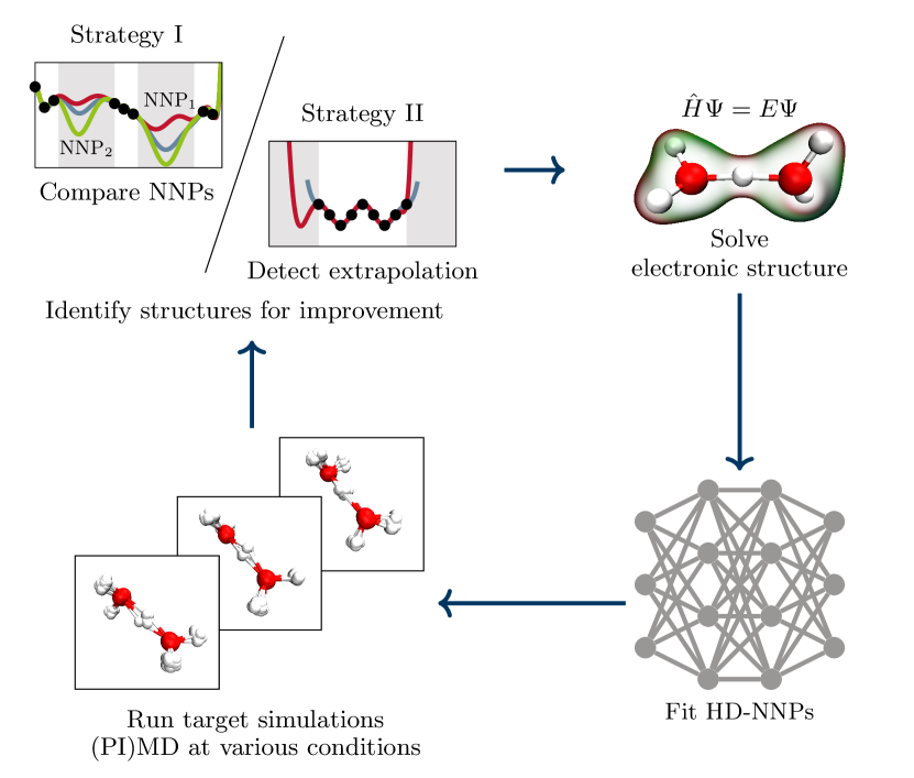
Figure 2: Schematic illustration of the four general steps in the developed automated fitting procedure. First, an ensemble of physically relevant structures is generated (lower left corner). At the start of the automated process, this is achieved with DFT based “on–the–fly” MD and PIMD simulation techniques, while later the preliminary NNPs can be utilized for this step. Afterwards, relevant structures for an improvement of the potential energy surface are selected either by comparison of two NNPs (Strategy I) or by detection of points with extrapolation problems (Strategy II) to improve regions of the surface that are underrepresented in the training set, highlighted in gray (upper left corner). Only for these selected configurations, explicit electronic structure calculations with the chosen reference method, in this case coupled cluster theory, are performed (upper right corner) to provide additional reference values for the training set. Afterwards, the two NNPs are refitted to the enhanced coupled cluster training set (lower right corner) and the cycle starts over by gathering new physically relevant structures (lower left corner), which can eventually be generated using the preliminary coupled cluster NNPs once they are sufficiently stable to run MD and PIMD simulations.

Using this approach, the most representative points of the starting ensemble are selected in an unbiased and efficient way. In addition, this allows one to keep the number of expensive coupled cluster reference calculations to a minimum. However, the selected points are not yet optimal for the high level reference method since DFT based structures are expected to differ from those provided by the reference method, i.e. they are biased with respect to those given by the desired (but unknown) coupled cluster surface. Therefore, the boundaries of the network are improved by expanding the configuration space of the training set in a next step. This is achieved by running a variety of simulations at different conditions and with different sampling methods, but now employing the preliminary coupled cluster based NNP. These simulations include all possible target approaches, such as classical and path integral molecular dynamics and enhanced sampling methods for which the final coupled cluster NNP is going to be used. As before, PIMD sampling needs to be included at this point if the quantum nature of the nuclei shall be accounted for in future uses of the NNP. This is necessary since classical MD can not provide the correct frequency dependent quantum fluctuations all the way from low (intermolecular) to high (intramolecular) frequencies, which usually leads to dissociation of molecular clusters if the temperature is increased up to the point to reach the classical limit in case of the highest modes of the system.

During these simulations, points that are subject to extrapolation are identified by comparison of the structural information encoded by the atom–centered symmetry functions to the training set (called “Strategy II” in Fig. 2). In case the NNP based simulation leaves the range of the training set, that particular configuration is needed for an improvement of the network and is selected for an explicit reference calculation. After sufficiently many such points (but as few as e.g. 20) have been identified, the simulations are aborted and new coupled cluster reference calculations are performed to improve the training set only where required. Afterwards, a new NNP is fitted that now has the capability to reliably predict the energy of the selected configurations. Thus, the simulations can be resumed to identify further points needed for an improvement. Utilizing the preliminary NNP for these simulations provides several advantages. First of all, a variety of different conditions can be explored and representative configurations sampled without problems due to the inexpensive functional relation of the NNP that is many orders of magnitude faster than the DFT based description of the electronic structure. This allows one, in addition, to reach rather long time scales and to generate statistically uncorrelated new configurations. At the same time, the preliminary NNP is approaching the coupled cluster reference over time, which ensures convergence. In practice, the majority of reference points is selected based on strategy I, since the DFT based structures usually provide a rather balanced sampling of configuration space. Still, strategy II is fundamentally important in order to gauge the NNP towards the coupled cluster PES and to provide truly uncorrelated new structures at various conditions.

After sufficiently many uncorrelated representative structures at different conditions and with a variety of sampling techniques have been generated, the training set needs to be further refined as shown in the following. While the boundaries of the network were iteratively improved, it is still possible that “holes” are present in the data set. Therefore, the above described automated comparison of two networks is utilized again to identify regions in the training set that are not yet optimally represented. This is done for each of the different sampling techniques and conditions individually for the following reasons. First of all, the separated improvement allows for a high degree of parallelization of the search for additional structures, which speeds up the fitting procedure. In addition, the different simulations may sample various regions of the PES with very distinct energies. Thus, the separate improvement prevents that regions with rather small energy differences remain undetected. In this process, it is important to have sufficient overlap of the different ensembles in order to prevent “holes” in the training set. The automated process is completed once the difference of the networks for the predicted energies converges for all ensembles of structures. This indicates that the most representative configurations have been identified for all distinct conditions. Therefore, the different training points of all ensembles can be combined for a final fit of the NNP.

III Computational details

To generate the required initial set of reference structures as a starting point for our automated fitting procedure as described in the previous section, AIMD and AI-PIMD simulations Marx and Hutter (2009) of the protonated water clusters were performed from H3O+ to H9O4+, including also the uncharged H2O monomer. These simulations have been carried out with our in–house developer’s version of the CP2k program package CP2 (2019); Hutter et al. (2014) in 9 to 20 Å cubic boxes with nonperiodic cluster boundary conditions. The electronic structure was described by the RPBE exchange correlation density functional Hammer, Hansen, and Nørskov (1999) together with the D3 dispersion correction Grimme et al. (2010) using the two–body terms and zero damping as evaluated on–the–fly using the Quickstep module VandeVondele et al. (2005). The charge density was represented on a grid up to a plane wave cutoff of 500 Ry. The TZV2P basis set together with Goedecker–Teter–Hutter pseudopotentials to replace the core electrons of the oxygen atoms Goedecker, Teter, and Hutter (1996) was used for the description of the Kohn–Sham orbitals. The SCF cycles were converged to an error of $\epsilon_{\text{SCF}}=10^{-7}\leavevmode\nobreak\ \text{Ha}$. This electronic structure setup has been shown repeatedly to provide reliable properties of water and is therefore the ideal starting point for our fitting procedure Morawietz and Behler (2013); Forster-Tonigold and Groß (2014); Morawietz et al. (2016). For each molecule at least $100\text{\,}\mathrm{ps}$ AIMD and $25\text{\,}\mathrm{ps}$ AI-PIMD trajectories were generated (after additional $2.5\text{\,}\mathrm{ps}$ equilibration periods in each case) to sample representative configurations with a time step of $0.25\text{\,}\mathrm{fs}$ at a temperature of $300\text{\,}\mathrm{K}$, where in the case of the AI-PIMD simulations the path integral has been discretized using 6 Trotter replicas. In case of the AI-PIMD simulations, the PIGLET algorithm Ceriotti and Manolopoulos (2012) was applied to sample the canonical quantum distribution, while for AIMD a massive Nosé–Hoover chain thermostat with a chain length of 5 was employed. For H9O4+, simulations starting from the four established isomers were performed in order to generate relevant configurations also for the higher energy isomers. From these reference ensembles we extracted configurations separated by $10\text{\,}\mathrm{fs}$ that serve as the basis for the generation of the NNP potentials based on DFT as outlined above.

The accurate reference energies were calculated via CCSD(T) by employing the explicitly correlated F12a method Adler, Knizia, and Werner (2007); Knizia, Adler, and Werner (2009) to correct for the basis set incompleteness error. In addition, size consistent scaling of the triples suggested in Ref. 69 was employed together with the aug-cc-pVTZ basis set Kendall, Jr, and Harrison (1992); Woon and Dunning Jr. (1994) for the calculation of the energies. This so-called CCSD(T*)-F12a/aug-cc-pVTZ electronic structure setup has been shown to provide energies close to the complete basis set (CBS) limit Knizia, Adler, and Werner (2009). All reference calculations were performed with the Molpro program packageWerner et al. (2015).

The NNP architecture is designed as detailed in the following. A set of symmetry functions for each element are chosen to transform the coordinates of the system to the input vectors for the atomic NNs. We chose the parameters of the symmetry functions for the final NNP according to Ref. 73, which have been optimized for the description of water. The largest cutoff in this set is about 6.5 Å for both, oxygen and hydrogen atoms. Therefore, the set of symmetry functions provide a global description of the chosen clusters since no atoms outside the cutoff radii are present, which could give rise to long-range electrostatic interactions that could not be covered by the NNP. The values of each symmetry function were centered around the respective average value of the training set and normalized to values between zero and one. These vectors serve as the input for the atomic NNs, which consist in all cases of two hidden layers with 30 nodes each, and yield the atomic energy contributions that sum up to the total energy. Bias nodes with weight parameters $b$ were attached to all layers but the input layer. The hyperbolic tangent was employed in all hidden layers except the output layer, where a linear activation function for the output layer prevents a confined range of output values. The NNPs are constructed by first splitting the set of CCSD(T*)-F12a/aug-cc-pVTZ reference data into a training set (90%) and an independent test set (10%). Subsequently, the weight parameters of the NNs were iteratively optimized to minimize the error of the training set, while the test set provides an estimate for the transferability to structures not included in the training set and is used to detect over fitting. Learning was achieved by optimizing the weights according to the adaptive global extended Kalman filter Shah, Palmieri, and Datum (1992); Blank and Brown (1994); Witkoskie and Doren (2005) as implemented in our in–house program RuNNer Behler et al. . Further details including the complete description of the NNP and all of its optimized parameters can be found in the supporting information.

The MD and PIMD simulations at different conditions using the generated NNPs were performed with our in-house NNP extension of the CP2k program package CP2 (2019); Hutter et al. (2014). These consist of simulations at temperatures of 10, 30, 70, 100, 200, 300, and $600\text{\,}\mathrm{K}$ for the MD simulations with otherwise the same settings as specified before for the AIMD simulations. For the PIMD simulations sampling of the quantum partition function at 1.67, 50, and $300\text{\,}\mathrm{K}$ was performed using PIGLET thermostatting with 512, 124, and 16 Trotter beads, respectively. During these MD as well as PIMD simulations, extrapolated points were identified when two consecutive structures were outside the range of the symmetry functions in the training set of the networks. In such a case, the simulations were aborted and new simulations were automatically started with a different random number seed. New electronic structure calculations were performed after 20 such extrapolating structures have been selected and the NNPs were re-fitted to the updated training set. Finally, a run time up to $8\text{\,}\mathrm{ns}$ with a time step of $0.5\text{\,}\mathrm{fs}$ and $0.5\text{\,}\mathrm{ns}$ with a time step of $0.25\text{\,}\mathrm{fs}$ under all above mentioned conditions were generated without occurrence of extrapolations for the classical and quantum description of the nuclei, respectively, using NNP-MD and NNP-PIMD.

In the case of the tetramer, additional enhanced sampling simulations based on constrained MD techniques were performed to incorporate rearrangements between the different isomers which involve high energy barriers. After careful analysis of the minimum energy pathway, obtained by the zero temperature string method E, Ren, and Vanden-Eijnden (2002), the OOO angle $\angle_{\text{OOO}}$ was identified as the most promising reaction coordinate to describe the isomerization of the Eigen complex to the Zundel–like state. Classical MD and quantum PIMD simulations were constrained via the “RATTLE” algorithm Andersen (1983) from 30 to 125^∘ in 40 angular steps. MD simulations were performed at temperatures of 200, 100, and $50\text{\,}\mathrm{K}$ via thermostatting using a Nosé–Hover chain thermostat. In the case of the PIMD simulations, the constraint was applied exclusively to the centroid following earlier work on free energy calculations in the path integral formalism Gillan (1987); Voth, Chandler, and Miller (1989); Walker and Michaelides (2010). Quantum simulations at 200 and $100\text{\,}\mathrm{K}$ were performed by thermostatting via the PILE Langevin thermostat Ceriotti et al. (2010), were the path integral was discretized using 32 and 64 replicas, respectively.

In order to validate the accuracy of the final NNP for production runs, classical MD simulations were performed at $300\text{\,}$ and $600\text{\,}\mathrm{K}$, while quantum PIMD simulations were carried out at $1.67\text{\,}$ and $300\text{\,}\mathrm{K}$. All trajectories were propagated for $25\text{\,}\mathrm{ps}$ with otherwise the same settings as for the above mentioned simulations. Afterwards, the last $100$ points of these trajectories were re-evaluated with the coupled cluster reference method to directly compare the performance of the NNP to the exact reference.

IV Neural Network Potential of Protonated Water Clusters

IV.1 Automated Neural Network Fitting Procedure

In order to develop a neural network potential that can be applied for the description of protonated water clusters from the monomer, H3O+, up to the tetramer, H9O4+, DFT based simulations were performed at $300\text{\,}\mathrm{K}$ to sample both the classical and quantum configuration space of all clusters using on–the–fly AIMD and AI-PIMD simulations, respectively. The water monomer, H2O, was also explicitly considered in these simulations to provide the correct description of the dissociation products of the protonated water clusters in the final NNP. For the largest cluster, H9O4+, all four known isomers (Eigen, Ring, Zundel-c and Zundel-t, see below for details) were used as the starting point of these simulations. Afterwards, at least $100\,000$ uncorrelated structures are extracted from these simulations for each cluster to serve as the basis of the automated NNP fitting procedure as outlined in the previous section. For every cluster size, the iterative selection of the most relevant configurations both for the classical and the quantum DFT ensembles were performed using at least $80$ refining stages. In each refining stage, the energies of $50\,000$ configurations were evaluated with two NNPs and the $20$ points with largest energy differences were added to the training set except at the beginning, when $20$ random structures were chosen to start. Afterwards, the training sets of the classical and quantum ensembles were combined and preliminary neural networks were fitted for each cluster individually.

In the next step, the boundaries of these networks were expanded in order to extend the configuration space of the reference set by running classical and quantum trajectories at different conditions. These consist of simulations at temperatures of 10, 30, 70, 100, 200, 300, and $600\text{\,}\mathrm{K}$ for classical nuclei, as well as 1.67, 50, and $300\text{\,}\mathrm{K}$ for quantum nuclei. During these simulations, extrapolated points were identified and iteratively added until sufficiently long trajectories under all above mentioned conditions were generated for the classical and quantum description of the nuclei, respectively. Recall that only a few configurations are selected based on this strategy, while the major contribution of reference points is selected based on the comparison of two NNPs. However, it is still a fundamentally important step in order to gauge the DFT based structures to the coupled cluster configuration space. In the case of the tetramer, additional enhanced sampling simulations based on thermodynamic integration were performed to incorporate rearrangements via higher–lying energetic barriers between the different isomers. All the computational details of these simulations and also the neural network specification as well as details on the coupled cluster reference calculations are presented in Sec. III. In a next step, the training sets of the respective clusters were refined by the same iterative comparison of two networks as before until the differences between the networks was converged. Afterwards, all reference calculations of all clusters were combined for a final fit of the neural network potential. In order to investigate if this final NNP has reached its asymptotic limit with respect to the size of the training set, or if the model would benefit from additional data, we analyzed the learning curves for the final data set in the supporting information. This analysis shows that the model is very close to its asymptotic accuracy and the automated fitting protocol is therefore considered to be converged.

Table I: Root mean square error of the energies per atom for the full data set (“All”) and for each individual cluster size. The values refer to the training set, while the numbers in parentheses correspond to the structures in the independent test set which are not considered in the fit of the neural network and thus provide an unbiased estimate of the predictive power.

Data	Number	RMSE
set	of structures	(kJ/mol)/atom
All	49242 (5470)	0.06 (0.08)
H2O	5933 (660)	0.03 (0.03)
H3O+	6489 (711)	0.05 (0.05)
H5O2+	8869 (1057)	0.07 (0.09)
H7O3+	9356 (973)	0.07 (0.08)
H9O4+	18595 (2069)	0.06 (0.10)

Overall, around $55\,000$ configurations for which coupled cluster energy calculations were carried out have been selected during the automated fitting procedure for all clusters in total. Roughly $50\,000$ of these points were used for the training of the final network, while the remaining $5000$ configurations have been used to access the transferability of the fit in an independent test set. Compared to standard approaches for the representation of a comparable PES, considerably less computationally demanding reference calculations were required to converge the PES, which is a considerable reduction of the computational cost. This clearly highlights the advantages of the automated selection of the training points over traditional approaches based for example on grids. The contribution of each individual cluster to the total training and test set is summarized in Table I. As seen therein, the higher number of degrees of freedom with increasing cluster size is well incorporated in the final reference set. In addition, the root mean squared error (RMSE) per atom is included in the table which for the total fit is around $0.06\text{\,}\mathrm{kJ}\text{\,}{\mathrm{mol}}^{-1}$ per atom. This error corresponds to a total energy error of $0.8\text{\,}\mathrm{kJ}\text{\,}{\mathrm{mol}}^{-1}$ and is thus much better than chemical accuracy (being 1 kcal/mol or about $4\text{\,}\mathrm{kJ}\text{\,}{\mathrm{mol}}^{-1}$) even for the largest considered cluster, which thus underlines the high quality of the fit. Furthermore, the fitting error is stable over the different cluster sizes, indicating that all of them are represented with similar accuracy. Last but not least, the error does not deteriorate significantly for the test set, which has not been considered during the fit, and thus provides an estimate of the transferability of the fitted potential.

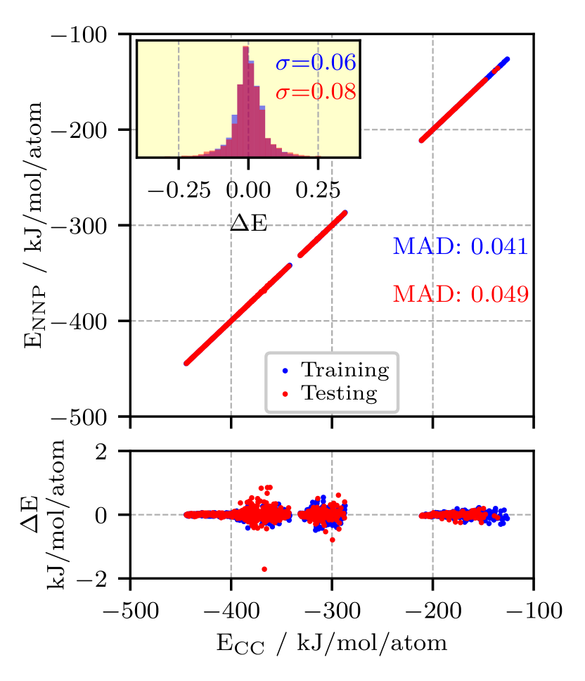
Figure 3: Correlation of the energy per atom from explicit CCSD(T*)-F12a/aug-cc-pVTZ calculations (CC) and the NNP predictions for the final reference data set, see text. The mean absolute difference (MAD) for the training and test set are given in blue and red, respectively. The lower panel shows the energy differences between coupled cluster reference and NNP prediction over the whole range of reference energies, while the inset in the upper panel shows the histograms of the energy differences including the corresponding standard deviations $\sigma$ in the respective color.

The resulting correlation between the reference CCSD(T*)-F12a/aug-cc-pVTZ (see Sec. III for details) energies per atom and the final NNP energies for the training and test sets is shown in Fig. 3. All considered points feature almost perfect correlation over the full range of energy values. Note that the gaps in the range of energies are a result of describing different cluster sizes with one and the same NNP, which is thus demonstrated to be capable of describing these very distinct clusters with one set of fitted parameters. The lower panel of the figure quantifies the deviation of the predicted energies over the whole range of the reference set. These are consistently small, for both the training and test set shown in blue and red colors, respectively. To further illustrate the accuracy of the fit, the histogram of these energy differences is shown in the upper inset of Fig. 3. It features a very narrow distribution for both, the training and test set with a standard deviation (which is equal to the RMSE) of around $0.08\text{\,}\mathrm{kJ}\text{\,}{\mathrm{mol}}^{-1}$ per atom. This error compares well with usual fitting errors of similarly complex hydrogen bonded clusters.

Overall, these results demonstrate that NNPs obtained from an automated procedure are able to represent highly complex potential energy landscapes including different system sizes with very high precision and are therefore ideally suited to reproduce the coupled cluster reference landscape. At the same time, the evaluation of the network is many orders of magnitude faster than the explicit electronic structure calculation. A reference calculation for the largest considered cluster, H9O4+, takes on the order of seven hours on a single core with rather high memory demands. The evaluation of the NNP can be performed in around $0.1\text{\,}\mathrm{ms}$, thus about $10^{8}$ times faster at roughly the same accuracy. This opens the door for systematic investigations of these systems using essentially exact interactions as provided by CCSD(T*)-F12a/aug-cc-pVTZ theory. The applicability of NNPs for the description of differently sized clusters has already been confirmed for DFT based potentials of water clusters Morawietz, Sharma, and Behler (2012); Morawietz and Behler (2013) and also for protonated water clusters Natarajan, Morawietz, and Behler (2015). However, these networks were additionally optimized to structure dependent forces acting on the nuclei during the fit, producing very similar results for the energies as presented above.

For the present study, the usage of forces is unfortunately out of scope, since the calculation of forces for coupled cluster theory are increasingly more demanding especially for the largest considered cluster which contains 13 atoms. To specifically test, if forces would further improve the accuracy of our fit, we therefore resorted to the following strategy: For the hydronium cation, H3O+, the evaluation of the forces is still feasible using the CCSD(T*)-F12a/aug-cc-pVTZ method. Therefore, the forces for all hydronium structures in our data set were explicitly calculated and two test networks were afterwards trained to this data. The first one utilizes the forces during the optimization, while the second one is trained to energies only. Afterwards, the test and training error for both fits can be compared to analyze the differences. For both fits very similar test and training errors were obtained for the energies. In addition, the error on the forces is very similar in both fits, although the force information was not used for one of the networks. The usage of forces, if available, would clearly be able to further reduce the number of required reference calculations (yet at the expense of strongly increasing the computational effort per reference configuration). However, they do not further improve the quality of our fit, if already sufficiently many training points are in the reference set.

In summary, the extension to the coupled cluster reference using only the training on energies provides results almost indistinguishable from the reference method. In addition, the automated assembly of the training set ensures that the procedure selects sufficiently many points for the representation of the PES and significantly reduces the number of required reference calculations. It also allows one to easily transfer this methodology to other systems and to readily develop new potentials.

Table II: Binding energy $E_{\text{bind}}$ in kcal/mol (units were chosen for direct comparison with Ref. 12) for selected stationary–point structures of protonated water clusters from H3O+ to H9O4+ optimized using the neural network potential (NNP) and the CCSD(T*)-F12a/aug-cc-pVTZ reference (CC). Here, $|$NNP-CC$|$ is the absolute difference between the two methods and $M$ is the number of water monomers in the cluster. Note that for the hydronium cation ($M=1$), $E_{\text{bind}}$ denotes the energy difference between H3O+ and the water monomer. The structures optimized with the NNP are depicted (those from CC optimization would be indistinguishable), were oxygen atoms are red and hydrogen atoms are white. The labels that are used throughout the text include an asterisk, if the shown configuration is the global minimum of the respective cluster size.

$M$	Structure	Label	Method	$E_{\text{bind}}$
1			NNP	-171.4
		C${}_{\text{3v}}^{*}$	CC	-171.5
			$|$NNP-CC$|$	0.037
2			NNP	-34.0
		C${}_{\text{2}}^{*}$	CC	-34.0
			$|$NNP-CC$|$	0.084
3			NNP	-57.7
		W3${}^{*}_{1}$	CC	-57.6
			$|$NNP-CC$|$	0.044
3			NNP	-57.7
		W32	CC	-57.6
			$|$NNP-CC$|$	0.063
4			NNP	-77.5
		Eigen∗	CC	-77.5
			$|$NNP-CC$|$	0.017
4			NNP	-73.5
		Ring	CC	-73.5
			$|$NNP-CC$|$	0.021
4			NNP	-73.6
		Zundel-c	CC	-73.6
			$|$NNP-CC$|$	0.014
4			NNP	-73.5
		Zundel-t	CC	-73.5
			$|$NNP-CC$|$	0.061

IV.2 Stationary Points and Vibrational Frequencies

To further validate the quality of the final neural network PES, structural and energetic properties of a set of optimized stationary–point structures obtained from the NNP are compared to the CCSD(T*)-F12a/aug-cc-pVTZ reference data (CC). In Table II the binding energies of the local minima for the hydronium cation, H3O+, up to the protonated water tetramer, H9O4+, are provided for both methods. For that purpose, all shown stationary points were first optimized with the NNP and then reoptimized using the coupled cluster reference, resulting into essentially indistinguishable structures for all species. The binding energy, calculated as usual from

$$E_{\text{bind}}(\text{H}^{+}(\cf{H2O})_{n})= E(\text{H}^{+}(\cf{H2O})_{n})-$$

$$(n-1)E(\cf{H2O})-E(\cf{H3O+})$$ (1)

based on the energies of the individually optimized clusters as obtained using the respective methods, is in very good agreement between the coupled cluster reference and the NNP. Even the largest energy difference between CCSD(T*)-F12a/aug-cc-pVTZ reference and NNP is found to not exceed $0.1\text{\,}\mathrm{kcal}\text{\,}{\mathrm{mol}}^{-1}$. This fitting error is already in the order of the remaining intrinsic uncertainty of the F12 coupled cluster method that is used and is at the level of state–of–the–art PES fits such as those relying on permutationally invariant polynomials Braams and Bowman (2009). Last but not least, the remaining fitting error does not systematically deteriorate with increasing system size, indicating very high quality representations for all included cluster sizes and isomers within a single NNP.

Since the NNP has been optimized using only the energy, the first derivative, i.e. the forces, are also important quantities to be tested. This particular validation has been done explicitly for the hydronium cation, but is out of scope for the larger clusters. Let us therefore focus on the curvature of the PES around the global minima of the different clusters, which is directly probed by the harmonic normal mode frequencies. As can be seen in Fig. 4, all investigated clusters show almost perfect agreement between the coupled cluster reference and the NNP. Overall, the mean absolute difference between the two methods is around $10\text{\,}{\mathrm{cm}}^{-1}$, which furthermore supports the rather high quality of the fit; note that this corresponds to about $0.1\text{\,}\mathrm{kJ}\text{\,}{\mathrm{mol}}^{-1}$ or $0.03\text{\,}\mathrm{kcal}\text{\,}{\mathrm{mol}}^{-1}$ and is thus in line with the reported energy errors. This is a strong indication that the forces of all clusters are also well described by the final NNP, which is in agreement with previous studies on a wide range of systems showing usually a very good representation of the forces.

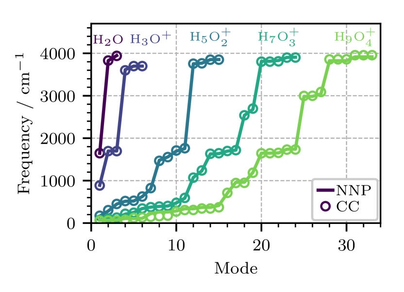
Figure 4: Comparison of the harmonic normal mode frequencies of the equilibrium structures corresponding to the global minima (depicted in Fig. II) as obtained using the neural network potential (NNP) and the coupled cluster (CC) reference. All global minima have been optimized with the respective method.

IV.3 Potential Energy Scans

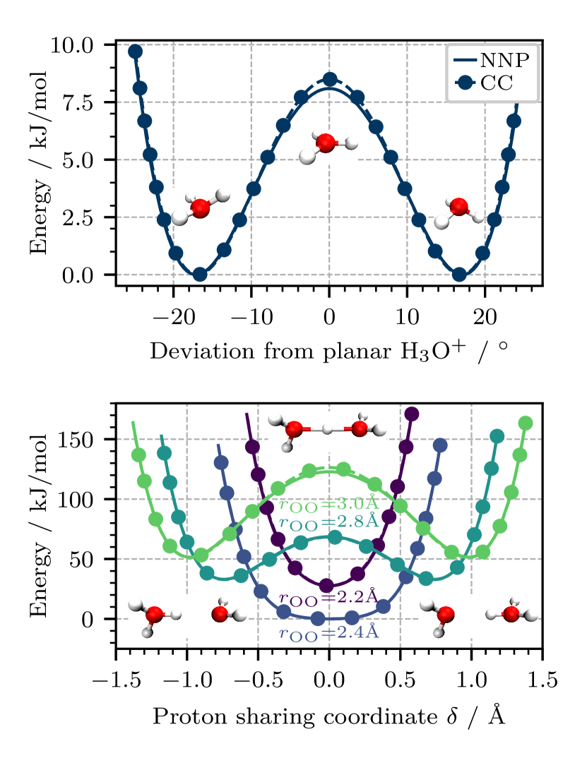
Figure 5: Scans of the potential energy profile obtained from the neural network potential (NNP) in comparison to the coupled cluster (CC) reference (marked with circles) for the hydronium and Zundel cation, H3O+ and H5O2+, respectively. Top: Scan of the potential energy of the hydronium cation along the inversion pathway of the umbrella motion where the reaction coordinate is defined as the dihedral angle of the four atoms which provides the deviation from planarity of the molecule; note that the OH bond distances are kept at the value of the minimum energy configuration. Bottom: Scans of the potential energy of the Zundel cation along the proton sharing (transfer) coordinate $\delta$ with the oxygen distance $r_{\text{OO}}$ constrained at different values as indicated; note that the OH bond distances of the dangling hydrogen atoms and their orientation are conserved with respect to the minimum energy structure. All energies are shown relative to the respective minimum energy structures (which is given by the global minimum around $r_{\text{OO}}=2.4$ Å for the Zundel cation).

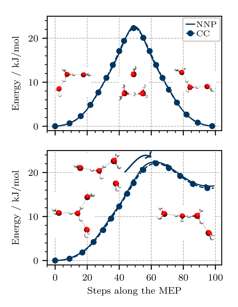
Figure 6: Potential energy profiles of the H7O3+ (top) and H9O4+ (bottom) clusters along selected minimum energy paths (MEP) for important isomerization reactions (represented by the respective reactant, transition and product state configurations) obtained using the zero temperature string method on the neural network potential (NNP). The coupled cluster (CC) reference was obtained by recomputing the energies along the NNP paths at representative points and are marked with circles. The arrow in the bottom panel indicates the position of the upper-left configuration at the maximum of that reaction coordinate. All energies are shown relative to the respective equilibrium structures.

After having confirmed that stationary point structures and corresponding harmonic frequencies are well reproduced by the NNP, larger non–equilibrium regions of the PES are now investigated in detail and compared to coupled cluster data. For that purpose, scans of the potential energy along different reaction coordinates are shown for the hydronium and Zundel cation in Fig. 5. For the hydronium complex, the umbrella-type interconversion motion along the inversion coordinate was chosen, which results in a planar transition state with D${}_{\text{3h}}$ symmetry. As seen in the top panel of Fig. 5, the energy profile as a function of the deviation from this planar transition state results in two equal minima at around $\pm 18^{\circ}$ that are separated by a barrier of around $8\text{\,}\mathrm{kJ}\text{\,}{\mathrm{mol}}^{-1}$. The NNP is able to reproduce this profile with very good accuracy, although small deviations from the coupled cluster reference of about $0.3\text{\,}\mathrm{kJ}\text{\,}{\mathrm{mol}}^{-1}$ can be detected in the transition state region, yet these differences are well within chemical accuracy.

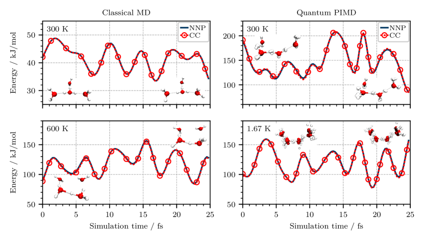
Figure 7: Potential energy along classical MD (left) and one replica of quantum PIMD (right) trajectories of the protonated water tetramer at $300\text{\,}\mathrm{K}$ (top) and $600\text{\,}\mathrm{K}$ (bottom-left) as well as $1.67\text{\,}\mathrm{K}$ (bottom-right) in the Eigen (top-left), Zundel-c (right), and Ring (bottom-left) conformation using the neural network potential (NNP). The coupled cluster (CC) reference was obtained by recomputing the energies along the NNP trajectories and are shown as red dotted lines (with a few circles added since the CC energies mostly superimpose the NNP data). All energies are reported relative to the Eigen equilibrium structure. The included snapshots depict the initial and final configurations in the short trajectory window that is covered (see text).

For the Zundel cation, the energy profile along the proton transfer coordinate $\delta$ (defined as the difference between the two oxygen–proton distances) is computed for different fixed oxygen–oxygen distances as indicated in the figure. By variation of the oxygen–oxygen distance it is possible to drive this system from a symmetric single-well hydrogen bond situation to an asymmetric double-well energy profile for larger oxygen–oxygen distances as seen in the bottom panel of Fig. 5. The equilibrium structure of this system corresponds to an OO distance close to 2.4 Å for which the broad anharmonic minimum with a centered proton position is observed in that figure. All other OO distances probe regions higher in energy, reaching relative energies of up to $150\text{\,}\mathrm{kJ}\text{\,}{\mathrm{mol}}^{-1}$ and mapping a proton transfer barrier as high as $75\text{\,}\mathrm{kJ}\text{\,}{\mathrm{mol}}^{-1}$ for the largest distance considered, $r_{\text{OO}}=3.0$ Å. For this system, essentially perfect agreement between the NNP and the coupled cluster reference is observed over the full energy range explored. These different scans of potential energy profiles corresponding to large-amplitude rearrangements show that the NNP is able to describe very different regions of the PES with convincing accuracy for two representative species, H3O+ and H5O2+.

In order to analyze similar non–equilibrium regions also for the larger clusters, H7O3+ and H9O4+, the zero temperature string method was applied using the NNP to compute minimum energy paths (MEPs) that connect two isomers of the different clusters. With this approach, the MEP for the rearrangement of the protonated water trimer from the W3₁ isomer to an equivalent W3₁ isomer with a different central H3O+ unit (see top panel of Fig. 6 for configurations) was obtained using the NNP. For the protonated water tetramer, a similar isomerization reaction transforms the Eigen cation to a linear hydrogen bonded complex that contains a central Zundel-like motif as depicted in the bottom panel of Fig. 6. Having determined the configurations along these MEPs based on the NNP, a set of single-point energies along these pathways were calculated using the coupled cluster reference method. The resulting NNP versus CC comparison of the two potential energy profiles is depicted in Fig. 6. In case of the protonated water trimer the transfer of one of the dangling water molecules to the other dangling water via a three–membered ring results in a degenerate W3₁ isomer structure of H7O3+. This rearrangement reaction is accompanied by proton transfer and features a reaction barrier of about $23\text{\,}\mathrm{kJ}\text{\,}{\mathrm{mol}}^{-1}$ which is well reproduced by the NNP. A very similar reaction leads in the larger protonated water tertramer to isomerization from the Eigen to a Zundel-like conformation. This process is characterized by a similar barrier height as the water transfer in the trimer of around $23\text{\,}\mathrm{kJ}\text{\,}{\mathrm{mol}}^{-1}$, however leading to an energetically higher-lying H9O4+ isomer in this case. Again, the NNP and coupled cluster reference provide essentially identical reaction profiles with only very minor differences.

IV.4 Molecular Dynamics and Path Integral Simulations

After having confirmed that also reaction pathways which drive these complexes far away from important stationary-points structures are well reproduced by the NNP, we finally validate the performance of the network when used in computer simulations with classical and quantum nuclear motion, i.e. for molecular dynamics and path integral simulation techniques. We recall that the performance of the NNP for truly uncorrelated configurations has been already validated based on the independent training set that was build up during the automated fitting process and, therefore, reflects vastly different conditions. In practice, however, it is also important to relate this accuracy to the fluctuations as generated during production simulations in order to explicitly validate the stability of the NNP in practical applications. For that purpose, the largest cluster, H9O4+, was simulated for $25\text{\,}\mathrm{ps}$ via classical MD and path integral MD employing the NNP at $1.67\text{\,}\mathrm{K}$ (PIMD), $300\text{\,}\mathrm{K}$ (MD and PIMD), as well as $600\text{\,}\mathrm{K}$ (MD).

The classical MD trajectories were initialized at the Eigen conformer, while the PIMD runs were started at the Zundel-c conformation to probe different regions of the PES. Note that in the high temperature classical simulation a variety of rearrangements are observed, leading in the end of the $25\text{\,}\mathrm{ps}$ to a configuration close to the Ring isomer. The computational details of these simulations can be found in Sec. III. Afterwards, the last $100$ steps of these trajectories were reevaluated with the coupled cluster reference to assess the quality of the NNP during the simulations. The resulting energy profiles are depicted in Fig. 7. Overall, the energy fluctuations are well reproduced and very good agreement between the coupled cluster reference and the NNP is observed. It can therefore be concluded that the NNP is also able to reliably describe protonated water clusters during classical MD and quantum PIMD simulations at various conditions covering very low and high temperatures, where configurations that fluctuate far away from the optimized stationary–point structures and MEPs are encountered.

It is important to note that such NNP simulations can be routinely performed on a normal desktop machine in a few minutes. Thus, this approach renders coupled cluster accuracy accessible for exhaustive exploration of protonated water clusters with different sampling techniques and at various conditions.

V Conclusions and Outlook

In conclusion, a systematic and fully automated procedure to efficiently parameterize potential energy surfaces for finite sized clusters employing high–dimensional neural network potentials has been developed. This NNP fitting procedure provides convincing agreement with the highly accurate reference electronic structure method, which is coupled cluster theory up to perturbative triples in an essentially converged basis set when used in conjunction with the F12 explicitly correlated wavefunction ansatz, namely CCSD(T*)-F12a/aug-cc-pVTZ. The flexibility of the underlying functional relation provided by the neural network ansatz allows one to easily identify deficiencies in the training set which can be used to systematically improve the potential while keeping the required total number of computationally demanding reference calculations to a minimum. This enables fast, automated and accurate development of NNPs and therefore overcomes the obstacles of traditional fitting approaches.

For the chosen protonated water clusters from the monomer to the tetramer, not only configurations close to equilibrium structures as characterized by stationary points and small–amplitude oscillations, but also non–equilibrium regions of the potential energy landscape are described with essentially the same accuracy using the same NNP for the four clusters. This holds true also for rearrangement reactions of these clusters involving proton transfer as well as other interconversion pathways. In addition, the NNP is equally well suited for the usage in classical molecular dynamics as well as for simulations including the quantum nature of nuclei from ultra-low to ambient to high temperature. Overall, the presented procedure will open the door to study many other intriguing systems at a converged description of the interactions in a straight–forward manner.

Supporting Information

See the Supporting Information for the details on the specific NNP formalism used, a full description of the specific architecture together with all optimized parameters of the developed NNP, as well as for complementary analyses of the learning curves for the final data set. In addition, all coupled cluster reference calculations are provided as Supporting Information free of charge on the ACS Publications website.