Discrete Vector Calculus and Helmholtz Hodge Decomposition for Classical Finite Difference Summation by Parts Operators

Abstract

In this article, discrete variants of several results from vector calculus are studied for classical finite difference summation by parts operators in two and three space dimensions. It is shown that existence theorems for scalar/vector potentials of irrotational/solenoidal vector fields cannot hold discretely because of grid oscillations, which are characterised explicitly. This results in a non-vanishing remainder associated to grid oscillations in the discrete Helmholtz Hodge decomposition. Nevertheless, iterative numerical methods based on an interpretation of the Helmholtz Hodge decomposition via orthogonal projections are proposed and applied successfully. In numerical experiments, the discrete remainder vanishes and the potentials converge with the same order of accuracy as usual in other first order partial differential equations. Motivated by the successful application of the Helmholtz Hodge decomposition in theoretical plasma physics, applications to the discrete analysis of magnetohydrodynamic (MHD) wave modes are presented and discussed.

AMS subject classification. 65N06, 65M06, 65N35, 65M70, 65Z05

1 Introduction

The Helmholtz Hodge decomposition of a vector field into irrotational and solenoidal components and their respective scalar and vector potentials is a classical result that appears in many different variants both in the traditional fields of mathematics and physics and more recently in applied sciences like medical imaging [53]. Especially in the context of classical electromagnetism and plasma physics, the Helmholtz Hodge decomposition has been used for many years to help analyse turbulent velocity fields [28, 5] or separate current systems into source-free and irrotational components [20, 22, 19, 21]. Numerical implementations can be useful for different tasks, as described in the survey article [7] and references cited therein. Some recent publications concerned with (discrete) Helmholtz Hodge decompositions are [4, 2, 30].

The main motivation for this article is the analysis of numerical solutions of hyperbolic balance/conservation laws such as the (ideal) magnetohydrodynamic (MHD) equations. Since the Helmholtz Hodge decomposition is a classical tool for the (theoretical) analysis of these systems, it is reasonable to assume that it can be applied fruitfully also in the discrete context.

For the hyperbolic partial differential equations of interest, summation by parts (SBP) operators provide a means to create stable and conservative discretisations mimicking energy and entropy estimates available at the continuous level, cf. [60, 13] and references cited therein. While SBP operators originate in the finite difference (FD) community [29, 55], they include also other schemes such as finite volume (FV) [38, 39], discontinuous Galerkin (DG) [17, 12], and the recent flux reconstruction/correction procedure via reconstruction schemes [24, 47].

SBP operators are constructed to mimic integration by parts discretely. Such mimetic properties of discretisations can be very useful to transfer results from the continuous level to the discrete one and have been of interest in various forms [25, 33, 43]. In this article, the focus will lie on finite difference operators, in particular on nullspace consistent ones. Similarly, (global) spectral methods based on Lobatto Legendre nodes can also be used since they satisfy the same assumptions.

Several codes applied in practice for relevant problems of fluid mechanics or plasma physics are based on collocated SBP operators. To the authors’ knowledge, the most widespread form of SBP operators used in practice are such collocated ones [60, 13]. These are easy to apply and a lot of effort has gone into optimising such schemes [34, 35]. Since this study is motivated by the analysis of numerical results obtained using widespread SBP operators resulting in provably stable methods, it is natural to consider classical collocated SBP operators. The novel numerical analysis provided in this article shows that a discrete Helmholtz Hodge decomposition and classical representation theorems of divergence/curl free vector fields cannot hold discretely in this setting. Even such a negative result is an important contribution, not least since the reason for the failure of these theorems from vector calculus for classical SBP operators is analysed in detail, showing the importance of explicitly characterised grid oscillations. Based on this analysis, numerical evidence is reported, showing that the negative influence of grid oscillations vanishes under grid refinement for smooth data. Moreover, means are developed to cope with the presence of such adversarial grid oscillations.

This article is structured as follows. Firstly, the concept of summation by parts operators is briefly reviewed in Section 2. Thereafter, classical existence theorems for scalar/vector potentials of irrotational/solenoidal vector fields are studied in the discrete context in Section 3. It will be shown that these representation theorems cannot hold discretely. Furthermore, the kernels of the discrete curl and divergence operators will be characterised via the images of the discrete gradient and curl operators and some additional types of grid oscillations. After a short excursion to the discrete characterisation of vector fields that are both divergence and curl free as gradients of harmonic functions in Section 4, the discrete Helmholtz decomposition is studied in Section 5. It will be shown that classical SBP operators cannot mimic the Helmholtz Hodge decomposition $u=\operatorname{grad}\varphi+\operatorname{curl}v$ discretely. Instead, the remainder $r=u-\operatorname{grad}\varphi-\operatorname{curl}v$ will in general not vanish in the discrete setting. Nevertheless, this remainder in associated with certain grid oscillations and converges to zero, as shown in numerical experiments in Section 6. Additionally, applications to the analysis of MHD wave modes are presented and discussed. Finally, the results are summed up and discussed in Section 7 and several directions of further research are described.

2 Summation by Parts Operators

In the following, finite difference methods on Cartesian grids will be used. Hence, the one dimensional setting is described at first. Throughout this article, functions at the continuous level are denoted using standard font, e.g. $u$, and discrete grid functions are denoted using boldface font, e.g. $\boldsymbol{u}$, independently on whether they are scalar or vector valued.

The given domain $\Omega=[x_{L},x_{R}]$ is discretised using a uniform grid with nodes $x_{L}=x_{1}<x_{2}<\dots<x_{N}=x_{R}$ and a function $u$ on $\Omega$ is represented discretely as a vector $(\boldsymbol{u}^{(a)})_{a}$, where the components are the values at the grid nodes, i.e. $\boldsymbol{u}^{(a)}=u(x_{a})$. Since a collocation setting is used, the grid is the same for every (vector or scalar valued) function and both linear and nonlinear operations are performed componentwise. For example, the product of two functions $u$ and $v$ is represented by the Hadamard product of the corresponding vectors, i.e. $(\boldsymbol{u}\boldsymbol{v})^{(a)}=\boldsymbol{u}^{(a)}\boldsymbol{v}^{(a)}$.

Definition 2.1.

An SBP operator with order of accuracy $p\in\mathbb{N}$ on $\Omega=[x_{L},x_{R}]\subset\mathbb{R}$ consists of the following components.

• A discrete derivative operator $D$, approximating the derivative $\partial_{x}u$ as $D\boldsymbol{u}$ with order of accuracy $p$.

• A symmetric and positive definite mass matrix $M$, approximating the scalar product on $L^{2}(\Omega)$ via

  $$\boldsymbol{u}^{T}M\boldsymbol{v}=\left\langle{\boldsymbol{u},\,\boldsymbol{v}}\right\rangle_{M}\approx\left\langle{u,\,v}\right\rangle_{L^{2}(\Omega)}=\int_{\Omega}u\cdot v.$$ (1)

• A boundary operator $E$, approximating the difference of boundary values as in the fundamental theorem of calculus as $u(x_{R})v(x_{R})-u(x_{L})v(x_{L})$ via $\boldsymbol{u}^{T}E\boldsymbol{v}$ with order of accuracy $p$.

• Finally, the SBP property

  $$MD+D^{T}M=E$$ (2)

  has to be fulfilled.

The SBP property (2) ensures that integration by parts is mimicked discretely as

$$\begin{array}[]{ccc}\underbrace{\boldsymbol{u}^{T}MD\boldsymbol{v}+\boldsymbol{u}^{T}D^{T}M\boldsymbol{v}}&=&\underbrace{\boldsymbol{u}^{T}E\boldsymbol{v},}\\ \rotatebox{90.0}{$\!\approx\;$}&&\rotatebox{90.0}{$\!\!\approx\;$}\\ \overbrace{\int_{x_{L}}^{x_{R}}u\,(\partial_{x}v)+\int_{x_{L}}^{x_{R}}(\partial_{x}u)\,v}&=&\overbrace{u\,v\big{|}_{x_{L}}^{x_{R}}},\end{array}$$ (6)

In the following, finite difference operators on nodes including the boundary points will be used. In that case, $E=\operatorname{diag}(-1,0,\dots,0,1)$.

For the numerical tests, only diagonal norm SBP operators are considered, i.e. those SBP operators with diagonal mass matrices $M$, because of their improved properties for (semi-) discretisations [57, 54, 14]. In this case, discrete integrals are evaluated using the quadrature provided by the weights of the diagonal mass matrix [23]. While there are also positive results for dense norm operators, the required techniques are more involved [46, 44, 8, 11]. However, the techniques and results of this article do not depend on diagonal mass matrices.

For classical diagonal norm SBP operators, the order of accuracy is $2p$ in the interior and $p$ at the boundaries [29, 31], allowing a global convergence order of $p+1$ for hyperbolic problems [59, 56, 58]. Here, SBP operators will be referred to by their interior order of accuracy $2p$.

Example 2.2.

The classical second order accurate SBP operators are

$$D=\frac{1}{2\Delta x}\begin{pmatrix}-2&2\\ -1&0&1\\ &\ddots&\ddots&\ddots\\ &&-1&0&1\\ &&&-2&2\end{pmatrix},\qquad M=\Delta x\begin{pmatrix}\frac{1}{2}\\ &1\\ &&\ddots\\ &&&1\\ &&&&\frac{1}{2}\end{pmatrix},$$ (7)

where $\Delta x$ is the grid spacing. Thus, the first derivative is given by the standard second order central derivative in the interior and by one sided derivative approximations at the boundaries.

SBP operators are designed to mimic the basic integral theorems of vector calculus (fundamental theorem of calculus, Gauss’ theorem, Stokes’ theorem) in the given domain $\Omega$ (but not necessarily on subdomains of $\Omega$). However, this mimetic property does not suffice for the derivations involving scalar and vector potentials in the following. Hence, nullspace consistency will be used as additional mimetic property that has also been used in [58, 32].

Definition 2.3.

An SBP derivative operator $D$ is nullspace consistent, if the nullspace/kernel of $D$ is $\operatorname{ker}D=\operatorname{span}\left\{\boldsymbol{1}\right\}$.

Remark 2.4.

A consistent derivative operator $D$ satisfies $\operatorname{span}\left\{\boldsymbol{1}\right\}\subseteq\operatorname{ker}D$. Some undesired behaviour can occur if $\operatorname{ker}D\neq\operatorname{span}\left\{\boldsymbol{1}\right\}$, cf. [58, 32, 45].

In multiple space dimensions, tensor product operators will be used, i.e. the one dimensional SBP operators are applied accordingly in each dimension. In the following, $\operatorname{I}_{s}$, $s\in\left\{x,y,z\right\}$, are identity matrices and $D_{s},M_{s},E_{s}$, $s\in\left\{x,y,z\right\}$, are one dimensional SBP operators in the corresponding coordinate directions.

Definition 2.5.

In two space dimensions, the tensor product operators are

$$\begin{gathered}\begin{aligned} D_{1}&=D_{x}\otimes\operatorname{I}_{y},&D_{2}&=\operatorname{I}_{x}\otimes D_{y},\\ E_{1}&=E_{x}\otimes M_{y},&E_{2}&=M_{x}\otimes E_{y},\end{aligned}\\ M=M_{x}\otimes M_{y},\end{gathered}$$ (8)

and the vector calculus operators are

$$\operatorname{grad}=\begin{pmatrix}D_{1}\\ D_{2}\end{pmatrix},\quad\operatorname{rot}=\begin{pmatrix}D_{2}\\ -D_{1}\end{pmatrix},\quad\operatorname{curl}=\begin{pmatrix}-D_{2},D_{1}\end{pmatrix},\quad\operatorname{div}=\begin{pmatrix}D_{1},D_{2}\end{pmatrix}.$$ (9)

Remark 2.6.

In two space dimensions, $\operatorname{curl}$ maps vector fields to scalar fields and $\operatorname{rot}$ maps scalar fields to vector fields. In three space dimensions, both operations correspond to the classical curl of a vector field.

Definition 2.7.

In three space dimensions, the tensor product operators are

$$\begin{gathered}\begin{aligned} D_{1}&=D_{x}\otimes\operatorname{I}_{y}\otimes\operatorname{I}_{z},&D_{2}&=\operatorname{I}_{x}\otimes D_{y}\otimes\operatorname{I}_{z},&D_{3}&=\operatorname{I}_{x}\otimes\operatorname{I}_{y}\otimes D_{z},\\ E_{1}&=E_{x}\otimes M_{y}\otimes M_{z},&E_{2}&=M_{x}\otimes E_{y}\otimes M_{z},&E_{3}&=M_{x}\otimes M_{y}\otimes E_{z}.\end{aligned}\\ M=M_{x}\otimes M_{y}\otimes M_{z},\end{gathered}$$ (10)

and the vector calculus operators are

$$\operatorname{grad}=\begin{pmatrix}D_{1}\\ D_{2}\\ D_{3}\end{pmatrix},\quad\operatorname{curl}=\begin{pmatrix}0&-D_{3}&D_{2}\\ D_{3}&0&-D_{1}\\ -D_{2}&D_{1}&0\end{pmatrix},\quad\operatorname{div}=\begin{pmatrix}D_{1},D_{2},D_{3}\end{pmatrix}.$$ (11)

Remark 2.8.

The standard tensor product discretisations of vector calculus operators given above satisfy $\operatorname{div}\operatorname{curl}=0$ (or $\operatorname{div}\operatorname{rot}=0$) and $\operatorname{curl}\operatorname{grad}=0$, since the discrete derivative operators commute, i.e. $D_{j}D_{i}=D_{i}D_{j}$.

3 Scalar and Vector Potentials

Classical results of vector calculus in three space dimensions state that (under suitable assumptions on the regularity of the domain and the vector fields)

• a vector field $u$ is curl free if and only if $u$ has a scalar potential $\varphi$, i.e. $u=\operatorname{grad}\varphi$,

• a vector field $u$ is divergence free if and only if $u$ has a vector potential $v$, i.e. $u=\operatorname{curl}v$.

Using modern notation, these classical theorems can be formulated as follows, cf. [18, Theorem I.2.9], [51, Corollary 2] and [27, Lemma 4.4]. In the following, $\Omega$ is always assumed to be a bounded rectangle/cuboid in $\mathbb{R}^{d}$, $d\in\left\{2,3\right\}$.

Theorem 3.1.

A vector field $u\in L^{2}(\Omega)^{d}$ satisfies $\operatorname{curl}u=0$ if and only if there exists a scalar potential $\varphi\in H^{1}(\Omega)$ satisfying $u=\operatorname{grad}\varphi$.

Theorem 3.2.

A vector field $u\in L^{2}(\Omega)^{d}$ satisfies $\operatorname{div}u=0$ if and only if

• there exists a potential $v\in H^{1}(\Omega)$ satisfying $u=\operatorname{rot}v$ if $d=2$,

• there exists a vector potential $v\in H(\operatorname{curl};\Omega)$ satisfying $u=\operatorname{curl}v$ if $d=3$.

Here, the rotation/curl of a scalar field $v$ is defined as $\operatorname{rot}v=(\partial_{2}v,-\partial_{1}v)$.

In the rest of this section, discrete analogues of these theorems will be studied for SBP operators. Before theorems characterising the discrete case can be proved, some preliminary results have to be obtained at first.

3.1 Grid Oscillations

For a nullspace consistent SBP derivative operator $D$, the kernel of its adjoint operator $D^{*}=M^{-1}D^{T}M$ will play an important role in the following.

Lemma 3.3.

For a nullspace consistent SBP derivative operator $D$ in one space dimension, $\dim\operatorname{ker}D^{*}=1$.

Proof.

For $N$ grid nodes, $\dim\operatorname{ker}D^{*}=\dim(\operatorname{im}D)^{\perp}=N-\dim\operatorname{im}D=\dim\operatorname{ker}D=\dim\operatorname{span}\left\{\boldsymbol{1}\right\}=1$. ∎

Definition 3.4.

A fixed but arbitrarily chosen basis vector of $\operatorname{ker}D^{*}$ for a nullspace consistent SBP operator $D$ is denoted as $\boldsymbol{\mathrm{osc}}$. In two space dimensions,

$$\begin{gathered}\begin{aligned} \boldsymbol{\mathrm{osc}}_{1}&=\boldsymbol{\mathrm{osc}}_{x}\otimes\boldsymbol{1},&\boldsymbol{\mathrm{osc}}_{2}&=\boldsymbol{1}\otimes\boldsymbol{\mathrm{osc}}_{y},\end{aligned}\\ \boldsymbol{\mathrm{osc}}_{12}=\boldsymbol{\mathrm{osc}}_{x}\otimes\boldsymbol{\mathrm{osc}}_{y},\end{gathered}$$ (12)

and in three space dimensions

$$\begin{gathered}\begin{aligned} \boldsymbol{\mathrm{osc}}_{1}&=\boldsymbol{\mathrm{osc}}_{x}\otimes\boldsymbol{1}\otimes\boldsymbol{1},&\boldsymbol{\mathrm{osc}}_{2}&=\boldsymbol{1}\otimes\boldsymbol{\mathrm{osc}}_{y}\otimes\boldsymbol{1},&\boldsymbol{\mathrm{osc}}_{3}&=\boldsymbol{1}\otimes\boldsymbol{1}\otimes\boldsymbol{\mathrm{osc}}_{z},\\ \boldsymbol{\mathrm{osc}}_{12}&=\boldsymbol{\mathrm{osc}}_{x}\otimes\boldsymbol{\mathrm{osc}}_{y}\otimes\boldsymbol{1},&\boldsymbol{\mathrm{osc}}_{13}&=\boldsymbol{\mathrm{osc}}_{x}\otimes\boldsymbol{1}\otimes\boldsymbol{\mathrm{osc}}_{z},&\boldsymbol{\mathrm{osc}}_{23}&=\boldsymbol{1}\otimes\boldsymbol{\mathrm{osc}}_{y}\otimes\boldsymbol{\mathrm{osc}}_{z},\end{aligned}\\ \boldsymbol{\mathrm{osc}}_{123}=\boldsymbol{\mathrm{osc}}_{x}\otimes\boldsymbol{\mathrm{osc}}_{y}\otimes\boldsymbol{\mathrm{osc}}_{z}.\end{gathered}$$ (13)

The name $\boldsymbol{\mathrm{osc}}$ shall remind of (grid) oscillations, since the kernel of $D^{*}$ is orthogonal to the image of $D$ which contains all sufficiently resolved functions.

Example 3.5.

For the classical second order SBP operator of Example 2.2,

$$D^{*}=M^{-1}D^{T}M=\frac{1}{2\Delta x}\begin{pmatrix}-2&-2\\ 1&0&-1\\ &\ddots&\ddots&\ddots\\ &&1&0&-1\\ &&&2&2\end{pmatrix}\in\mathbb{R}^{N\times N},$$ (14)

and $\operatorname{ker}D^{*}=\operatorname{span}\left\{\boldsymbol{\mathrm{osc}}\right\}$, where

$$\begin{cases}\boldsymbol{\mathrm{osc}}^{(1)}=\boldsymbol{\mathrm{osc}}^{(3)}=\dots=\boldsymbol{\mathrm{osc}}^{(N)}=-\boldsymbol{\mathrm{osc}}^{(2)}=-\boldsymbol{\mathrm{osc}}^{(4)}=\dots=-\boldsymbol{\mathrm{osc}}^{(N-1)},&N\text{ odd},\\ \boldsymbol{\mathrm{osc}}^{(1)}=\boldsymbol{\mathrm{osc}}^{(3)}=\dots=\boldsymbol{\mathrm{osc}}^{(N-1)}=-\boldsymbol{\mathrm{osc}}^{(2)}=-\boldsymbol{\mathrm{osc}}^{(4)}=\dots=-\boldsymbol{\mathrm{osc}}^{(N)},&N\text{ even}.\end{cases}$$ (15)

Thus, $\boldsymbol{\mathrm{osc}}$ represents classical grid oscillations. Grid oscillations for the SBP derivative operators of [36] are visualised in Figure 1. These grid oscillations alternate between $+1$ and $-1$ in the interior of the domain. Near the boundaries, the values depend on the order and boundary closure of the scheme.

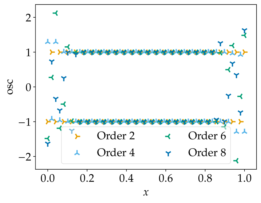
(a) $N=50$ grid points.

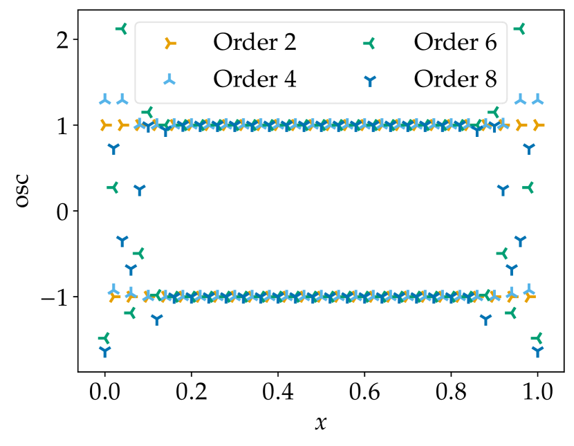
(b) $N=51$ grid points.

Figure 1: Grid oscillations for the SBP derivative operators of [36] and $N\in\left\{50,51\right\}$ grid points.

Example 3.6.

For a nodal Lobatto Legendre (global) spectral method using polynomials of degree $\leq p$ and their exact derivatives, grid oscillations are given by the highest Legendre mode existing on the grid. Indeed, grid oscillations have to be polynomials of degree $\leq p$, orthogonal to all polynomials of degree $\leq p-1$.

3.2 Two Space Dimensions

In this section, the kernels of the discrete divergence and curl operators will be characterised. It will become clear that scalar/vector potentials of discretely curl/divergence free vector fields exist if and only if no grid oscillations are present.

Theorem 3.7.

Suppose that nullspace consistent tensor product SBP operators are applied in two space dimensions. Then,

$$\dim\operatorname{im}\operatorname{grad}=N_{1}N_{2}-1<N_{1}N_{2}+1=\dim\operatorname{ker}\operatorname{curl}$$ (16)

and the kernel of the discrete curl operator can be decomposed into the direct orthogonal sum

$$\operatorname{ker}\operatorname{curl}=\operatorname{im}\operatorname{grad}\oplus\operatorname{span}\left\{\begin{pmatrix}\boldsymbol{\mathrm{osc}}_{1}\\ \boldsymbol{0}\end{pmatrix},\begin{pmatrix}\boldsymbol{0}\\ \boldsymbol{\mathrm{osc}}_{2}\end{pmatrix}\right\}.$$ (17)

Proof.

Since the operator is nullspace consistent, $\operatorname{ker}\operatorname{grad}=\operatorname{span}\left\{\boldsymbol{1}\right\}$ and

$$\dim\operatorname{im}\operatorname{grad}=N_{1}N_{2}-\dim\operatorname{ker}\operatorname{grad}=N_{1}N_{2}-1.$$ (18)

Similarly,

$$\dim\operatorname{ker}\operatorname{curl} =\dim\operatorname{ker}\begin{pmatrix}-D_{2},D_{1}\end{pmatrix}=\dim\left(\operatorname{im}\begin{pmatrix}-D_{2}^{*}\\ D_{1}^{*}\end{pmatrix}\right)^{\perp}$$ (19)

$$=2N_{1}N_{2}-\dim\operatorname{im}\begin{pmatrix}-D_{2}^{*}\\ D_{1}^{*}\end{pmatrix}=N_{1}N_{2}+\dim\operatorname{ker}\begin{pmatrix}-D_{2}^{*}\\ D_{1}^{*}\end{pmatrix}=N_{1}N_{2}+1.$$

Since tensor product derivative operators commute, $\operatorname{im}\operatorname{grad}\subseteq\operatorname{ker}\operatorname{curl}$. Additionally,

$$\operatorname{im}\operatorname{grad}=\operatorname{im}\begin{pmatrix}D_{1}\\ D_{2}\end{pmatrix}=\left(\operatorname{ker}\begin{pmatrix}D_{1}^{*},D_{2}^{*}\end{pmatrix}\right)^{\perp}=(\operatorname{ker}\operatorname{grad}^{*})^{\perp}$$ (20)

and the span in (17) is contained in $\operatorname{ker}\operatorname{grad}^{*}$. ∎

Theorem 3.8.

Suppose that nullspace consistent tensor product SBP operators are applied in two space dimensions. Then,

$$\dim\operatorname{im}\operatorname{rot}=N_{1}N_{2}-1<N_{1}N_{2}+1=\dim\operatorname{ker}\operatorname{div}$$ (21)

and the kernel of the discrete divergence operator can be decomposed into the direct orthogonal sum

$$\operatorname{ker}\operatorname{div}=\operatorname{im}\operatorname{rot}\oplus\operatorname{span}\left\{\begin{pmatrix}\boldsymbol{0}\\ \boldsymbol{\mathrm{osc}}_{1}\end{pmatrix},\begin{pmatrix}\boldsymbol{\mathrm{osc}}_{2}\\ \boldsymbol{0}\end{pmatrix}\right\}.$$ (22)

Proof.

The arguments are basically the same as in the proof of Theorem 3.7, since

$$\operatorname{rot}=\begin{pmatrix}D_{2}\\ -D_{1}\end{pmatrix}=\begin{pmatrix}0&\operatorname{I}\\ -\operatorname{I}&0\end{pmatrix}\begin{pmatrix}D_{1}\\ D_{2}\end{pmatrix}=\begin{pmatrix}0&\operatorname{I}\\ -\operatorname{I}&0\end{pmatrix}\operatorname{grad}$$ (23)

and

$$\operatorname{div}=\begin{pmatrix}D_{1},D_{2}\end{pmatrix}=\begin{pmatrix}-D_{2},D_{1}\end{pmatrix}\begin{pmatrix}0&-\operatorname{I}\\ \operatorname{I}&0\end{pmatrix}=\operatorname{curl}\begin{pmatrix}0&-\operatorname{I}\\ \operatorname{I}&0\end{pmatrix}.\qed$$ (24)

3.3 Scalar Potentials via Integrals in Two Space Dimensions

Theorem 3.7 shows that not every discretely curl free vector field is the gradient of a scalar potential and specifies even the orthogonal complement of $\operatorname{im}\operatorname{grad}$ in $\operatorname{ker}\operatorname{curl}$ in two space dimensions. In the continuous setting of classical vector calculus, scalar potentials are often constructed explicitly using integrals. Hence, it is interesting to review this construction and its discrete analogue, yielding another proof of (17).

Classically, a scalar potential of a (sufficiently smooth) curl free vector field $u$ in the box $[0,x_{1,\mathrm{max}}]\times[0,x_{2,\mathrm{max}}]$ can be defined via

$$\varphi(x)=\int_{0}^{x_{1}}u_{1}(\xi,0)\operatorname{d\!}\xi+\int_{0}^{x_{2}}u_{2}(x_{1},\eta)\operatorname{d\!}\eta.$$ (25)

Indeed, $\partial_{2}\varphi(x)=u_{2}(x)$ and

$$\partial_{1}\varphi(x)=u_{1}(x_{1},0)+\int_{0}^{x_{2}}\underbrace{\partial_{1}u_{2}}_{=\partial_{2}u_{1}}(x_{1},\eta)\operatorname{d\!}\eta=u_{1}(x_{1},x_{2}).$$ (26)

Consider now a discretely curl free vector field $\boldsymbol{u}$ perpendicular to $\operatorname{span}\left\{\begin{pmatrix}\boldsymbol{\mathrm{osc}}_{1}\\ \boldsymbol{0}\end{pmatrix},\begin{pmatrix}\boldsymbol{0}\\ \boldsymbol{\mathrm{osc}}_{2}\end{pmatrix}\right\}$, i.e. a discrete vector field $\boldsymbol{u}$ satisfying

$$D_{1}\boldsymbol{u}_{2}=D_{2}\boldsymbol{u}_{1},\qquad\boldsymbol{u}_{1}\perp\boldsymbol{\mathrm{osc}}_{1},\qquad\boldsymbol{u}_{2}\perp\boldsymbol{\mathrm{osc}}_{2}.$$ (27)

Since the second integral in (25) is the inverse of the partial derivative $\partial_{2}$, the discrete $\boldsymbol{u}_{2}$ must be in $\operatorname{im}D_{2}$ in order to mimic (25) discretely.

Lemma 3.9.

Suppose that nullspace consistent tensor product SBP operators are applied in two space dimensions. If the discrete vector field $\boldsymbol{u}$ satisfies (27), $\boldsymbol{u}_{i}\in\operatorname{im}D_{i}$, $i\in\left\{1,2\right\}$.

Proof.

It suffices to consider the case $i=2$ ($i=1$ is similar).

There are $\boldsymbol{v}_{2},\boldsymbol{w}_{2}$ such that $\boldsymbol{u}_{2}=D_{2}\boldsymbol{v}_{2}+\boldsymbol{w}_{2}$, where $\boldsymbol{w}_{2}\in(\operatorname{im}D_{2})^{\perp}=\operatorname{ker}D_{2}^{*}$. To show that $\boldsymbol{w}_{2}=\boldsymbol{0}$, use $D_{2}\boldsymbol{u}_{1}=D_{1}\boldsymbol{u}_{2}=D_{1}D_{2}\boldsymbol{v}_{2}+D_{1}\boldsymbol{w}_{2}$ and calculate

$$\mathinner{\!\left\lVert D_{1}\boldsymbol{w}_{2}\right\rVert}^{2}=\left\langle{D_{1}\boldsymbol{w}_{2},\,D_{2}\boldsymbol{u}_{1}-D_{1}D_{2}\boldsymbol{v}_{2}}\right\rangle=\left\langle{\boldsymbol{w}_{2},\,D_{1}^{*}D_{2}\boldsymbol{u}_{1}-D_{1}^{*}D_{1}D_{2}\boldsymbol{v}_{2}}\right\rangle\\ =\left\langle{\boldsymbol{w}_{2},\,D_{2}\bigl{(}D_{1}^{*}\boldsymbol{u}_{1}-D_{1}^{*}D_{1}\boldsymbol{v}_{2}\bigr{)}}\right\rangle=0.$$ (28)

Therefore, $\boldsymbol{w}_{2}\in\operatorname{ker}D_{1}=\operatorname{span}\left\{\boldsymbol{1}\right\}\otimes\mathbb{R}^{N_{2}}$. However, $\boldsymbol{w}_{2}\in\operatorname{ker}D_{2}^{*}=\mathbb{R}^{N_{1}}\otimes\operatorname{span}\left\{\boldsymbol{\mathrm{osc}}_{y}\right\}$ by definition. Hence, $\boldsymbol{w}_{2}\in\operatorname{span}\left\{\boldsymbol{1}\otimes\boldsymbol{\mathrm{osc}}_{y}\right\}=\operatorname{span}\left\{\boldsymbol{\mathrm{osc}}_{2}\right\}$. Finally, using $\boldsymbol{u}_{2}\perp\boldsymbol{\mathrm{osc}}_{2}$ yields

$$0=\left\langle{\boldsymbol{u}_{2},\,\boldsymbol{\mathrm{osc}}_{2}}\right\rangle=\left\langle{D_{2}\boldsymbol{v}_{2}+\boldsymbol{w}_{2},\,\boldsymbol{\mathrm{osc}}_{2}}\right\rangle=\left\langle{\boldsymbol{v}_{2},\,D_{2}^{*}\boldsymbol{\mathrm{osc}}_{2}}\right\rangle+\left\langle{\boldsymbol{w}_{2},\,\boldsymbol{\mathrm{osc}}_{2}}\right\rangle=\left\langle{\boldsymbol{w}_{2},\,\boldsymbol{\mathrm{osc}}_{2}}\right\rangle,$$ (29)

since $\boldsymbol{\mathrm{osc}}_{2}\in\operatorname{ker}D_{2}^{*}$. Thus, $\boldsymbol{w}_{2}=\boldsymbol{0}$. ∎

Next, discrete inverse operators of the partial derivatives are needed in order to mimic the integrals in (25). At first, the one dimensional setting will be studied in the following.

Consider a nullspace consistent SBP derivative operator $D$ on the interval $[0,x_{\mathrm{max}}]$ using $N$ grid points and the corresponding subspaces

$$V_{0}=\left\{\boldsymbol{u}\in\mathbb{R}^{N}\;\middle|\;\boldsymbol{u}(x=0)=0\right\},\quad V_{1}=\left\{\boldsymbol{u}\in\mathbb{R}^{N}\;\middle|\;\exists\boldsymbol{v}\in\mathbb{R}^{N}\colon\boldsymbol{u}=D\boldsymbol{v}\right\}.$$ (30)

Here and in the following, $\boldsymbol{u}(x=0)$ denotes the value of the discrete function $\boldsymbol{u}$ at the corresponding grid points. In the one-dimensional case, $\boldsymbol{u}(x=0)=\boldsymbol{u}^{(1)}$ is the first coefficient of $\boldsymbol{u}$. This notation is useful in several space dimensions to refer to values at hyperplanes and other subspaces.

Clearly, $D\colon V_{0}\to V_{1}$ is surjective. Because of nullspace consistency, $D\colon V_{0}\to V_{1}$ is even bijective and hence invertible. Denote the inverse operator as $D^{-1}\colon V_{1}\to V_{0}$. In multiple space dimensions, the discrete partial derivative operators and their inverse operators are defined analogously using tensor products. Now, everything is set to provide another proof of (17).

Lemma 3.10.

Suppose that nullspace consistent tensor product SBP operators are applied in two space dimensions. If the discrete vector field $\boldsymbol{u}$ satisfies (27), there is a discrete scalar potential $\boldsymbol{\varphi}$ of $\boldsymbol{u}$.

Corollary 3.11.

Suppose that nullspace consistent tensor product SBP operators are applied in two space dimensions. Then, $\dim\operatorname{ker}\operatorname{curl}=\dim\operatorname{im}\operatorname{grad}+2$.

Proof of Lemma 3.10.

By Lemma 3.9, $\boldsymbol{u}_{i}\in\operatorname{im}D_{i}$ and $D_{i}^{-1}\boldsymbol{u}_{i}$ is well-defined for $i\in\left\{1,2\right\}$. Define

$$\boldsymbol{\varphi}=(D_{1}^{-1}\boldsymbol{u}_{1})(x_{2}=0)\otimes\boldsymbol{1}+D_{2}^{-1}\boldsymbol{u}_{2}.$$ (31)

Here, $(D_{1}^{-1}\boldsymbol{u}_{1})(x_{2}=0)$ denotes the value of $D_{1}^{-1}\boldsymbol{u}_{1}$ in the $x_{2}=0$ hyperplane. Then,

$$D_{2}\boldsymbol{\varphi}=(\operatorname{I}_{x}\otimes D_{y})\boldsymbol{\varphi}=\boldsymbol{0}+(\operatorname{I}_{x}\otimes D_{y}D_{y}^{-1})\boldsymbol{u}_{2}=\boldsymbol{u}_{2}.$$ (32)

Moreover, using $D_{1}\boldsymbol{u}_{2}=D_{2}\boldsymbol{u}_{1}$,

$$D_{1}D_{2}^{-1}\boldsymbol{u}_{2}=(D_{x}\otimes\operatorname{I}_{y})(\operatorname{I}_{x}\otimes D_{y}^{-1})\boldsymbol{u}_{2}=D_{2}^{-1}D_{1}\boldsymbol{u}_{2}=D_{2}^{-1}D_{2}\boldsymbol{u}_{1}.$$ (33)

Since $D_{2}^{-1}$ is the inverse of $D_{2}$ for fields with zero initial values at $x_{2}=0$,

$$D_{1}\boldsymbol{\varphi}=(D_{x}\otimes\operatorname{I}_{y})\bigl{(}D_{x}^{-1}\boldsymbol{u}_{1}(x_{2}=0)\bigr{)}\otimes\boldsymbol{1}+D_{2}^{-1}D_{2}\boldsymbol{u}_{1}=\boldsymbol{u}_{1}(x_{2}=0)\otimes\boldsymbol{1}+D_{2}^{-1}D_{2}\boldsymbol{u}_{1}=\boldsymbol{u}_{1}.$$ (34)

Hence, $\boldsymbol{\varphi}$ is a scalar potential of $\boldsymbol{u}$ and (25) is mimicked discretely. ∎

3.4 Preliminary Results in Three Space Dimensions

Here, the kernels of the discrete divergence and curl operators will be studied in three space dimensions. Since the arguments seem to be more complicated than in the two-dimensional case because of the different structure of the curl operator, preliminary results are obtained at first. They will be improved using the same techniques presented in Section 3.3 afterwards.

Lemma 3.12.

Suppose that nullspace consistent tensor product SBP operators are applied in three space dimensions. Then,

$$\dim\operatorname{im}\operatorname{grad}=N_{1}N_{2}N_{3}-1<N_{1}N_{2}N_{3}+2\leq\dim\operatorname{ker}\operatorname{curl}$$ (35)

and the kernel of the discrete curl operator is a superspace of the direct orthogonal sum

$$\operatorname{ker}\operatorname{curl}\supseteq\operatorname{im}\operatorname{grad}\oplus\operatorname{span}\left\{\begin{pmatrix}\boldsymbol{\mathrm{osc}}_{1}\\ \boldsymbol{0}\\ \boldsymbol{0}\end{pmatrix},\begin{pmatrix}\boldsymbol{0}\\ \boldsymbol{\mathrm{osc}}_{2}\\ \boldsymbol{0}\end{pmatrix},\begin{pmatrix}\boldsymbol{0}\\ \boldsymbol{0}\\ \boldsymbol{\mathrm{osc}}_{3}\end{pmatrix}\right\}.$$ (36)

Proof.

For a nullspace consistent operator, $\operatorname{ker}\operatorname{grad}=\operatorname{span}\left\{\boldsymbol{1}\right\}$ and

$$\dim\operatorname{im}\operatorname{grad}=N_{1}N_{2}N_{3}-\dim\operatorname{ker}\operatorname{grad}=N_{1}N_{2}N_{3}-1.$$ (37)

Since tensor product derivative operators commute, $\operatorname{im}\operatorname{grad}\subseteq\operatorname{ker}\operatorname{curl}$. Additionally,

$$\operatorname{im}\operatorname{grad}=\operatorname{im}\begin{pmatrix}D_{1}\\ D_{2}\\ D_{3}\end{pmatrix}=\left(\operatorname{ker}\begin{pmatrix}D_{1}^{*},D_{2}^{*},D_{3}^{*}\end{pmatrix}\right)^{\perp}=(\operatorname{ker}\operatorname{grad}^{*})^{\perp}$$ (38)

and the span in (36) is contained in both $\operatorname{ker}\operatorname{grad}^{*}$ and $\operatorname{ker}\operatorname{curl}$. ∎

Lemma 3.13.

Suppose that nullspace consistent tensor product SBP operators are applied in three space dimensions. Then,

$$\dim\operatorname{im}\operatorname{curl}\leq 2N_{1}N_{2}N_{3}-2<2N_{1}N_{2}N_{3}+1=\dim\operatorname{ker}\operatorname{div}$$ (39)

and the kernel of the discrete divergence operator is a superspace of the direct orthogonal sum

$$\operatorname{ker}\operatorname{div}\supseteq\operatorname{im}\operatorname{curl}\oplus\operatorname{span}\left\{\begin{pmatrix}\boldsymbol{\mathrm{osc}}_{23}\\ \boldsymbol{0}\\ \boldsymbol{0}\end{pmatrix},\begin{pmatrix}\boldsymbol{0}\\ \boldsymbol{\mathrm{osc}}_{13}\\ \boldsymbol{0}\end{pmatrix},\begin{pmatrix}\boldsymbol{0}\\ \boldsymbol{0}\\ \boldsymbol{\mathrm{osc}}_{12}\end{pmatrix}\right\}.$$ (40)

Proof.

For a nullspace consistent operator,

$$\dim\operatorname{ker}\operatorname{div}=\dim\left(\operatorname{im}\begin{pmatrix}D_{1}^{*}\\ D_{2}^{*}\\ D_{3}^{*}\end{pmatrix}\right)^{\perp}=3N_{1}N_{2}N_{3}-\dim\operatorname{im}\begin{pmatrix}D_{1}^{*}\\ D_{2}^{*}\\ D_{3}^{*}\end{pmatrix}\\ =2N_{1}N_{2}N_{3}+\dim\operatorname{ker}\begin{pmatrix}D_{1}^{*}\\ D_{2}^{*}\\ D_{3}^{*}\end{pmatrix}=2N_{1}N_{2}N_{3}+1.$$ (41)

Since tensor product derivative operators commute, $\operatorname{im}\operatorname{curl}\subseteq\operatorname{ker}\operatorname{div}$. Additionally, $\operatorname{im}\operatorname{curl}=(\operatorname{ker}\operatorname{curl}^{*})^{\perp}$ and the span in (40) is contained in both $\operatorname{ker}\operatorname{curl}^{*}$ and $\operatorname{ker}\operatorname{div}$. ∎

3.5 Scalar Potentials via Integrals in Three Space Dimensions

The methods used in Section 3.3 to get scalar potential for discretely curl free vector fields can also be applied in three space dimensions. They can even be used to extend the preliminary results of the previous Section 3.4.

Consider a box $[0,x_{1,\mathrm{max}}]\times[0,x_{2,\mathrm{max}}]\times[0,x_{3,\mathrm{max}}]$. In the continuous setting, the analogue of (25) is

$$\varphi(x)=\int_{0}^{x_{1}}u_{1}(\xi,0,0)\operatorname{d\!}\xi+\int_{0}^{x_{2}}u_{2}(x_{1},\eta,0)\operatorname{d\!}\eta+\int_{0}^{x_{3}}u_{3}(x_{1},x_{2},\zeta)\operatorname{d\!}\zeta.$$ (42)

As in the two-dimensional case, $\boldsymbol{u}_{i}\in\operatorname{im}D_{i}$ is necessary to mimic (42) discretely. Here, the necessary conditions are

$$\forall i,j\in\left\{1,2,3\right\}\colon\qquad D_{i}\boldsymbol{u}_{j}=D_{j}\boldsymbol{u}_{i},\qquad\boldsymbol{u}_{i}\perp\boldsymbol{\mathrm{osc}}_{i}.$$ (43)

Lemma 3.14.

Suppose that nullspace consistent tensor product SBP operators are applied in three space dimensions. If the discrete vector field $\boldsymbol{u}$ satisfies (43), $\boldsymbol{u}_{i}\in\operatorname{im}D_{i}$, $i\in\left\{1,2,3\right\}$.

Proof.

Consider $i=1$ for simplicity. The other cases can be handled similarly.

There are $\boldsymbol{v}_{1},\boldsymbol{w}_{1}$ such that $\boldsymbol{u}_{1}=D_{1}\boldsymbol{v}_{1}+\boldsymbol{w}_{1}$, where $\boldsymbol{w}_{1}\in(\operatorname{im}D_{1})^{\perp}=\operatorname{ker}D_{1}^{*}$. To show that $\boldsymbol{w}_{1}=\boldsymbol{0}$, use $D_{1}\boldsymbol{u}_{j}=D_{j}\boldsymbol{u}_{1}=D_{j}D_{1}\boldsymbol{v}_{1}+D_{j}\boldsymbol{w}_{1}$ for $j\in\left\{2,3\right\}$ and calculate (without summing over $j$)

$$\mathinner{\!\left\lVert D_{j}\boldsymbol{w}_{1}\right\rVert}^{2}=\left\langle{D_{j}\boldsymbol{w}_{1},\,D_{1}\boldsymbol{u}_{j}-D_{j}D_{1}\boldsymbol{v}_{1}}\right\rangle=\left\langle{\boldsymbol{w}_{1},\,D_{j}^{*}D_{1}\boldsymbol{u}_{j}-D_{j}^{*}D_{j}D_{1}\boldsymbol{v}_{1}}\right\rangle\\ =\left\langle{\boldsymbol{w}_{1},\,D_{1}\bigl{(}D_{j}^{*}\boldsymbol{u}_{j}-D_{j}^{*}D_{j}\boldsymbol{v}_{1}\bigr{)}}\right\rangle=0.$$ (44)

Therefore, $\boldsymbol{w}_{1}\in\operatorname{ker}D_{2}\cap\operatorname{ker}D_{3}=\mathbb{R}^{N_{1}}\otimes\operatorname{span}\left\{\boldsymbol{1}\right\}\otimes\operatorname{span}\left\{\boldsymbol{1}\right\}$. However, $\boldsymbol{w}_{1}\in\operatorname{ker}D_{1}^{*}=\operatorname{span}\left\{\boldsymbol{\mathrm{osc}}_{x}\right\}\otimes\mathbb{R}^{N_{2}}\otimes\mathbb{R}^{N_{3}}$ by definition. Hence, $\boldsymbol{w}_{1}\in\operatorname{span}\left\{\boldsymbol{\mathrm{osc}}_{x}\otimes\boldsymbol{1}\otimes\boldsymbol{1}\right\}=\operatorname{span}\left\{\boldsymbol{\mathrm{osc}}_{1}\right\}$. Finally, using $\boldsymbol{u}_{1}\perp\boldsymbol{\mathrm{osc}}_{1}$ yields

$$0=\left\langle{\boldsymbol{u}_{1},\,\boldsymbol{\mathrm{osc}}_{1}}\right\rangle=\left\langle{D_{1}\boldsymbol{v}_{1}+\boldsymbol{w}_{1},\,\boldsymbol{\mathrm{osc}}_{1}}\right\rangle=\left\langle{\boldsymbol{v}_{1},\,D_{1}^{*}\boldsymbol{\mathrm{osc}}_{1}}\right\rangle+\left\langle{\boldsymbol{w}_{1},\,\boldsymbol{\mathrm{osc}}_{1}}\right\rangle=\left\langle{\boldsymbol{w}_{1},\,\boldsymbol{\mathrm{osc}}_{1}}\right\rangle,$$ (45)

since $\boldsymbol{\mathrm{osc}}_{1}\in\operatorname{ker}D_{1}^{*}$. Thus, $\boldsymbol{w}_{1}=\boldsymbol{0}$. ∎

Using Lemma 3.14 allows to prove

Lemma 3.15.

Suppose that nullspace consistent tensor product SBP operators are applied in three space dimensions. If the discrete vector field $\boldsymbol{u}$ satisfies (43), there is a discrete scalar potential $\boldsymbol{\varphi}$ of $\boldsymbol{u}$.

Corollary 3.16.

Suppose that nullspace consistent tensor product SBP operators are applied in three space dimensions. Then, $\dim\operatorname{ker}\operatorname{curl}=\dim\operatorname{im}\operatorname{grad}+3$.

Proof of Lemma 3.15.

By Lemma 3.9, $\boldsymbol{u}_{i}\in\operatorname{im}D_{i}$ and $D_{i}^{-1}\boldsymbol{u}_{i}$ is well-defined for $i\in\left\{1,2,3\right\}$. Define

$$\boldsymbol{\varphi}=(D_{1}^{-1}\boldsymbol{u}_{1})(x_{2}=x_{3}=0)\otimes\boldsymbol{1}\otimes\boldsymbol{1}+(D_{2}^{-1}\boldsymbol{u}_{2})(x_{3}=0)\otimes\boldsymbol{1}+D_{3}^{-1}\boldsymbol{u}_{3}.$$ (46)

Here, $(D_{1}^{-1}\boldsymbol{u}_{1})(x_{2}=x_{3}=0)$ denotes the value of $D_{1}^{-1}\boldsymbol{u}_{1}$ on the $x_{2}=x_{3}=0$ curve and $(D_{2}^{-1}\boldsymbol{u}_{2})(x_{3}=0)$ is a value in the $x_{3}=0$ plane. Then,

$$D_{3}\boldsymbol{\varphi}=(\operatorname{I}_{x}\otimes\operatorname{I}_{y}\otimes D_{z})\boldsymbol{\varphi}=\boldsymbol{0}+\boldsymbol{0}+(\operatorname{I}_{x}\otimes\operatorname{I}_{y}\otimes D_{z}D_{z}^{-1})\boldsymbol{u}_{3}=\boldsymbol{u}_{3}.$$ (47)

Using $D_{2}\boldsymbol{u}_{3}=D_{3}\boldsymbol{u}_{2}$ yields

$$D_{2}D_{3}^{-1}\boldsymbol{u}_{3}=D_{3}^{-1}D_{2}\boldsymbol{u}_{3}=D_{3}^{-1}D_{3}\boldsymbol{u}_{2}.$$ (48)

Since $D_{3}^{-1}$ is the inverse of $D_{3}$ for fields with zero initial values at $x_{3}=0$,

$$D_{2}\boldsymbol{\varphi}=\boldsymbol{0}+(\operatorname{I}_{x}\otimes D_{y}\otimes\operatorname{I}_{z})\bigl{(}(\operatorname{I}_{x}\otimes D_{y}^{-1})\boldsymbol{u}_{2}(x_{3}=0)\bigr{)}\otimes\boldsymbol{1}+D_{3}^{-1}D_{3}\boldsymbol{u}_{2}\\ =\boldsymbol{u}_{2}(x_{3}=0)\otimes\boldsymbol{1}+D_{3}^{-1}D_{3}\boldsymbol{u}_{2}=\boldsymbol{u}_{2}.$$ (49)

Similarly, inserting $D_{1}\boldsymbol{u}_{2}=D_{2}\boldsymbol{u}_{1}$ results in

$$D_{1}D_{2}^{-1}\boldsymbol{u}_{2}=D_{2}^{-1}D_{1}\boldsymbol{u}_{2}=D_{2}^{-1}D_{2}\boldsymbol{u}_{1}$$ (50)

and $D_{1}\boldsymbol{u}_{3}=D_{3}\boldsymbol{u}_{1}$ yields

$$D_{1}D_{3}^{-1}\boldsymbol{u}_{3}=D_{3}^{-1}D_{1}\boldsymbol{u}_{3}=D_{3}^{-1}D_{3}\boldsymbol{u}_{1}.$$ (51)

Using again that $D_{i}^{-1}$, $i\in\left\{2,3\right\}$, is the inverse of $D_{i}$ for fields with zero initial values at $x_{i}=0$,

$$D_{1}\boldsymbol{\varphi}=(D_{x}\otimes\operatorname{I}_{y}\otimes\operatorname{I}_{z})\bigl{(}D_{x}^{-1}\boldsymbol{u}_{1}(x_{2}=x_{3}=0)\bigr{)}\otimes\boldsymbol{1}\otimes\boldsymbol{1}+(D_{2}^{-1}D_{2}\boldsymbol{u}_{1})(x_{3}=0)\otimes\boldsymbol{1}+D_{3}^{-1}D_{3}\boldsymbol{u}_{1}\\ =\boldsymbol{u}_{1}(x_{2}=x_{3}=0)\otimes\boldsymbol{1}\otimes\boldsymbol{1}+\boldsymbol{u}_{1}(x_{3}=0)\otimes\boldsymbol{1}-\boldsymbol{u}_{1}(x_{2}=x_{3}=0)\otimes\boldsymbol{1}\otimes\boldsymbol{1}+D_{3}^{-1}D_{3}\boldsymbol{u}_{1}=\boldsymbol{u}_{1}.$$ (52)

Hence, $\boldsymbol{\varphi}$ is a scalar potential of $\boldsymbol{u}$ and (42) is mimicked discretely. ∎

Remark 3.17.

Similarly to the construction of the scalar potential $\varphi$ (42), a vector potential $v=(v_{1},v_{2},0)$ of a (sufficiently smooth) divergence free vector field $u$ can be constructed via

$$v_{1}(x)=\int_{0}^{x_{3}}u_{2}(x_{1},x_{2},\zeta)\operatorname{d\!}\zeta-\int_{0}^{x_{2}}u_{3}(x_{1},\eta,0)\operatorname{d\!}\eta,\qquad v_{2}(x)=-\int_{0}^{x_{3}}u_{1}(x_{1},x_{2},\zeta)\operatorname{d\!}\zeta.$$ (53)

Discrete versions can probably be obtained along the same lines.

3.6 Three Space Dimensions Revisited

Using the results of the previous Section 3.5, the following analogues in three space dimensions of Theorems 3.7 and 3.8 can be obtained. In particular, the inequalities in Lemmas 3.12 and 3.13 become equalities and scalar/vector potentials of discretely curl/divergence free vector fields exist if and only if no grid oscillations are present.

Theorem 3.18.

Suppose that nullspace consistent tensor product SBP operators are applied in three space dimensions. Then,

$$\dim\operatorname{im}\operatorname{grad}=N_{1}N_{2}N_{3}-1<N_{1}N_{2}N_{3}+2=\dim\operatorname{ker}\operatorname{curl}$$ (54)

and the kernel of the discrete curl operator can be decomposed into the direct orthogonal sum

$$\operatorname{ker}\operatorname{curl}=\operatorname{im}\operatorname{grad}\oplus\operatorname{span}\left\{\begin{pmatrix}\boldsymbol{\mathrm{osc}}_{1}\\ \boldsymbol{0}\\ \boldsymbol{0}\end{pmatrix},\begin{pmatrix}\boldsymbol{0}\\ \boldsymbol{\mathrm{osc}}_{2}\\ \boldsymbol{0}\end{pmatrix},\begin{pmatrix}\boldsymbol{0}\\ \boldsymbol{0}\\ \boldsymbol{\mathrm{osc}}_{3}\end{pmatrix}\right\}.$$ (55)

Proof.

Apply Lemma 3.12 and Corollary 3.16. ∎

Theorem 3.19.

Suppose that nullspace consistent tensor product SBP operators are applied in three space dimensions. Then,

$$\dim\operatorname{im}\operatorname{curl}=2N_{1}N_{2}N_{3}-2<2N_{1}N_{2}N_{3}+1=\dim\operatorname{ker}\operatorname{div}$$ (56)

and the kernel of the discrete divergence operator can be decomposed into the direct orthogonal sum

$$\operatorname{ker}\operatorname{div}=\operatorname{im}\operatorname{curl}\oplus\operatorname{span}\left\{\begin{pmatrix}\boldsymbol{\mathrm{osc}}_{23}\\ \boldsymbol{0}\\ \boldsymbol{0}\end{pmatrix},\begin{pmatrix}\boldsymbol{0}\\ \boldsymbol{\mathrm{osc}}_{13}\\ \boldsymbol{0}\end{pmatrix},\begin{pmatrix}\boldsymbol{0}\\ \boldsymbol{0}\\ \boldsymbol{\mathrm{osc}}_{12}\end{pmatrix}\right\}.$$ (57)

Proof.

Apply Lemma 3.13 and Corollary 3.16, using that $\dim\operatorname{im}\operatorname{curl}+\dim\operatorname{ker}\operatorname{curl}=3N_{1}N_{2}N_{3}$. ∎

3.7 Remarks on Numerical Implementations

Theorems 3.7, 3.8, 3.18, and 3.19 show that $\operatorname{ker}\operatorname{curl}=\operatorname{im}\operatorname{grad}$ and $\operatorname{ker}\operatorname{div}=\operatorname{im}\operatorname{curl}$ (or $\operatorname{ker}\operatorname{div}=\operatorname{im}\operatorname{rot}$ in two space dimensions) do not hold discretely. However, these relations become true when the kernels are restricted to the subspace of grid functions orthogonal to grid oscillations in either coordinate direction.

Hence, if potentials of curl/divergence free vector fields are sought, one has to remove these grid oscillations, e.g. by an orthogonal projection. Such a projection can be interpreted as a discrete filtering process, reducing the discrete norm induced by the mass matrix. For example, the operator filtering out all grid oscillations $\boldsymbol{\mathrm{osc}}_{i}$, $i\in\left\{1,\dots,d\right\}$, is given by

$$F\mathrel{\mathop{\ordinarycolon}}=\operatorname{I}-\sum_{i=1}^{d}\frac{\boldsymbol{\mathrm{osc}}_{i}\boldsymbol{\mathrm{osc}}_{i}^{T}M}{\mathinner{\!\left\lVert\boldsymbol{\mathrm{osc}}_{i}\right\rVert}_{M}^{2}}.$$ (58)

Theorem 3.20.

The filter operator $F$ (58) is an orthogonal projection with respect to the scalar product induced by $M$ and satisfies $\mathinner{\!\left\lVert F\right\rVert}\leq 1$, where the operator norm is induced by the discrete norm $\mathinner{\!\left\lVert\cdot\right\rVert}_{M}$.

Proof.

It suffices to note that grid oscillations in different coordinate directions are orthogonal, because

$$\boldsymbol{1}\in\operatorname{im}D_{i}\perp\operatorname{ker}D_{i}^{*}=\operatorname{span}\left\{\boldsymbol{\mathrm{osc}}_{i}\right\}.\qed$$ (59)

The approaches to construct scalar (and similarly vector) potentials in Sections 3.2 and 3.6 depend crucially on the satisfaction of $\operatorname{curl}\boldsymbol{u}=\boldsymbol{0}$ (or $\operatorname{div}\boldsymbol{u}=\boldsymbol{0}$) discretely. Hence, they can be ill-conditioned and numerical roundoff errors can influence the results, cf. [52] for a related argument concerning a “direct” and a “global linear algebra” approach to compute vector potentials. Moreover, they are not really suited for discrete Helmholtz Hodge decompositions targeted in Section 5. Hence, other approaches will be pursued in the following, cf. Section 5.1.

4 Characterisation of Divergence and Curl Free Functions

Combining Theorems 3.7, 3.8, 3.18, and 3.19 yields a characterisation of vector fields that are both divergence free and curl free. As before, the continuous case is described at first, cf. [51, Corollary 2, Theorem 2 and its proof].

Theorem 4.1.

For a vector field $u\in L^{2}(\Omega)^{d}$, the following conditions are equivalent.

1. $\operatorname{div}u=0$ and $\operatorname{curl}u=0$.

2. $u$ is the gradient of a harmonic function $\varphi\in H^{1}(\Omega)$, solving the Neumann problem

   $$\int_{\Omega}(\operatorname{grad}\varphi)\cdot(\operatorname{grad}\psi)=\int_{\partial\Omega}(u\cdot\nu)\psi,\quad\forall\psi\in H^{1}(\Omega).$$ (60)

Here, $\nu$ is the outer unit normal at $\partial\Omega$.

Note that the right hand side of (60) is well defined, because the trace of $\psi\in H^{1}(\Omega)$ is in $H^{1/2}(\partial\Omega)$ and the normal trace of $u\in H(\operatorname{div};\Omega)=\left\{u\in L^{2}(\Omega)\;\middle|\;\operatorname{div}u\in L^{2}(\Omega)\right\}$ is in $H^{-1/2}(\partial\Omega)$ [18, Theorem I.2.5].

Although the theorems guaranteeing the existence of scalar/vector potentials do not hold discretely, the characteristation of vector fields that are both divergence and curl free is similar to the one at the continuous level given by Theorem 4.1.

Theorem 4.2.

If nullspace consistent tensor product SBP operators are applied, the following conditions are equivalent for a grid function $\boldsymbol{u}$ in two or three space dimensions.

1. $\operatorname{div}\boldsymbol{u}=\boldsymbol{0}$ and $\operatorname{curl}\boldsymbol{u}=\boldsymbol{0}$.

2. $\boldsymbol{u}$ is the discrete gradient of a discretely harmonic function $\boldsymbol{\varphi}$, i.e. $D_{i}D_{i}\boldsymbol{\varphi}=\boldsymbol{0}$.

If $\operatorname{div}\boldsymbol{u}=\boldsymbol{0}$ and $\operatorname{curl}\boldsymbol{u}=\boldsymbol{0}$, the scalar potential $\boldsymbol{\varphi}$ can be determined as solution of the Neumann problem

$$D_{i}^{T}MD_{i}\boldsymbol{\varphi}=E_{i}\boldsymbol{u}_{i}.$$ (61)

Proof.

Since the grid oscillations appearing in $\operatorname{ker}\operatorname{div}$ are not in $\operatorname{ker}\operatorname{curl}$ and vice versa,

$$\operatorname{ker}\operatorname{div}\cap\operatorname{ker}\operatorname{curl}\subseteq\operatorname{im}\operatorname{grad}\cap\operatorname{im}\operatorname{rot}$$ (62)

in two space dimensions and

$$\operatorname{ker}\operatorname{div}\cap\operatorname{ker}\operatorname{curl}\subseteq\operatorname{im}\operatorname{grad}\cap\operatorname{im}\operatorname{curl}$$ (63)

in three space dimensions.

“i) $\iff$ ii)”: Because of $\boldsymbol{u}\in\operatorname{im}\operatorname{grad}$ and $\operatorname{div}\boldsymbol{u}=\boldsymbol{0}$, there is a scalar potential $\boldsymbol{\varphi}$ satisfying $\boldsymbol{u}_{i}=D_{i}\boldsymbol{\varphi}$ and $\boldsymbol{0}=D_{i}\boldsymbol{u}_{i}=D_{i}D_{i}\boldsymbol{\varphi}$. Additionally,

$$D_{i}^{T}MD_{i}\boldsymbol{\varphi}=E_{i}D_{i}\boldsymbol{\varphi}-MD_{i}D_{i}\boldsymbol{\varphi}=E_{i}\boldsymbol{u}_{i}.$$ (64)

Conversely, if $\boldsymbol{\varphi}$ is a discretely harmonic grid function and $\boldsymbol{u}_{i}=D_{i}\boldsymbol{\varphi}$, $\operatorname{div}\boldsymbol{u}=D_{i}\boldsymbol{u}_{i}=D_{i}D_{i}\boldsymbol{\varphi}=\boldsymbol{0}$ because $\boldsymbol{\varphi}$ is discretely harmonic. Additionally, $\operatorname{curl}\boldsymbol{u}=\boldsymbol{0}$, since $\boldsymbol{u}$ is the discrete gradient of $\boldsymbol{\varphi}$ and the discrete curl of a discrete gradient vanishes, cf. Remark 2.8.

A solution of the discrete Neumann problem (61) is determined uniquely up to an additive constant, since $\operatorname{ker}D_{i}^{T}MD_{i}=\operatorname{ker}\operatorname{grad}=\left\{\boldsymbol{1}\right\}$ for nullspace consistent SBP operators. Hence, $D_{i}^{T}MD_{i}$ is symmetric and positive semidefinite and a solution of the Neumann problem exists if and only if the right hand side is orthogonal to the kernel of $D_{i}^{T}MD_{i}$ (both with respect to the Euclidean standard inner product and not the one induced by $M$). This is the case if $D_{i}\boldsymbol{u}_{i}=\boldsymbol{0}$, since

$$\boldsymbol{1}^{T}E_{i}\boldsymbol{u}_{i}=\boldsymbol{1}^{T}(MD_{i}+D_{i}^{T}M)\boldsymbol{u}_{i}=\boldsymbol{1}^{T}MD_{i}\boldsymbol{u}_{i}.\qed$$ (65)

5 Variants of the Helmholtz Hodge Decomposition

There are several variants of the Helmholtz Hodge decomposition of a vector field $u\in L^{2}(\Omega)$, i.e. decompositions of $u$ into curl free and divergence free components, e.g.

$$\forall u\in L^{2}(\Omega)^{2}\;\exists\varphi\in H^{1}(\Omega),v\in H^{1}(\Omega)\colon\quad u=\operatorname{grad}\varphi+\operatorname{rot}v$$ (66)

in two space dimensions [18, Theorem I.3.2] and

$$\forall u\in L^{2}(\Omega)^{3}\;\exists\varphi\in H^{1}(\Omega),v\in H(\operatorname{curl};\Omega)\colon\quad u=\operatorname{grad}\varphi+\operatorname{curl}v$$ (67)

in three space dimensions [18, Corollary I.3.4], where additional (boundary) conditions are used to specify the potentials (e.g. uniquely up to an additive constant for the scalar potential $\varphi$) and guarantee that these decompositions are orthogonal in $L^{2}(\Omega)$. Discretely, such decompositions are not possible in general.

Theorem 5.1.

For nullspace consistent tensor product SBP operators, there are grid functions $\boldsymbol{u}$ such that

$$\begin{cases}\boldsymbol{u}\notin\operatorname{im}\operatorname{grad}+\operatorname{im}\operatorname{rot},&\text{ in two space dimensions},\\ \boldsymbol{u}\notin\operatorname{im}\operatorname{grad}+\operatorname{im}\operatorname{curl},&\text{ in three space dimensions}.\end{cases}$$ (68)

In particular,

$$\operatorname{span}\left\{\begin{pmatrix}\boldsymbol{\mathrm{osc}}_{12}\\ \boldsymbol{0}\end{pmatrix},\begin{pmatrix}\boldsymbol{0}\\ \boldsymbol{\mathrm{osc}}_{12}\end{pmatrix}\right\}\subseteq(\operatorname{im}\operatorname{grad}+\operatorname{im}\operatorname{rot})^{\perp}$$ (69)

in two space dimensions and

$$\operatorname{span}\left\{\begin{pmatrix}\boldsymbol{\mathrm{osc}}_{123}\\ \boldsymbol{0}\\ \boldsymbol{0}\end{pmatrix},\begin{pmatrix}\boldsymbol{0}\\ \boldsymbol{\mathrm{osc}}_{123}\\ \boldsymbol{0}\end{pmatrix},\begin{pmatrix}\boldsymbol{0}\\ \boldsymbol{0}\\ \boldsymbol{\mathrm{osc}}_{123}\end{pmatrix}\right\}\subseteq(\operatorname{im}\operatorname{grad}+\operatorname{im}\operatorname{curl})^{\perp}$$ (70)

in three space dimensions.

Proof.

Using Theorems 3.7 and 3.8,

$$\dim(\operatorname{im}\operatorname{grad}+\operatorname{im}\operatorname{rot})\leq\dim\operatorname{im}\operatorname{grad}+\dim\operatorname{im}\operatorname{rot}=2N_{1}N_{2}-2$$ (71)

in two space dimensions. In three space dimensions, Theorems  3.18 and 3.19 yield

$$\dim(\operatorname{im}\operatorname{grad}+\operatorname{im}\operatorname{curl})\leq\dim\operatorname{im}\operatorname{grad}+\dim\operatorname{im}\operatorname{curl}=3N_{1}N_{2}N_{3}-3.$$ (72)

Finally, note that grid oscillations are orthogonal to the image of SBP derivative operators. ∎

Remark 5.2.

In general, there is no equality in the subspace relations of Theorem 5.1. Up to now, no complete characterisation of $(\operatorname{im}\operatorname{grad}+\operatorname{im}\operatorname{curl})^{\perp}$ or $(\operatorname{im}\operatorname{grad})^{\perp}\cap(\operatorname{im}\operatorname{curl})^{\perp}=(\operatorname{ker}\operatorname{grad}^{*})\cap(\operatorname{ker}\operatorname{curl}^{*})$ has been obtained. In numerical experiments, some sort of grid oscillations always seem to be involved.

Nevertheless, it is possible to compute orthogonal decompositions of the form

$$\begin{cases}\boldsymbol{u}=\operatorname{grad}\boldsymbol{\varphi}+\operatorname{rot}\boldsymbol{v}+\boldsymbol{r},&\boldsymbol{r}\perp\operatorname{im}\operatorname{grad},\operatorname{im}\operatorname{rot},\quad\text{ \phantom{c}in two space dimensions},\\ \boldsymbol{u}=\operatorname{grad}\boldsymbol{\varphi}+\operatorname{curl}\boldsymbol{v}+\boldsymbol{r},&\boldsymbol{r}\perp\operatorname{im}\operatorname{grad},\operatorname{im}\operatorname{curl},\quad\text{ in three space dimensions}.\end{cases}$$ (73)

In the following, only the three dimensional case will be described. In two space dimensions, some occurrences of $\operatorname{curl}$ have to be substituted by $\operatorname{rot}$.

In the literature, variants of the Helmholtz Hodge decomposition in bounded domains are most often presented with an emphasis on boundary conditions, cf. [18, 10, 3, 51]. With this emphasis, the following two choices of boundary conditions appear most often in the literature.

Proposition 5.3.

Suppose $u\in L^{2}(\Omega)^{3}$.

1. There exist $\varphi\in H^{1}(\Omega)$ with $\int_{\Omega}\varphi=0$ and $v\in H(\Omega,\operatorname{curl})\cap H(\Omega,\operatorname{div})$ with $\operatorname{div}v=0$ and $\nu\times v|_{\partial\Omega}=0$ such that (73) with $r=0$ is an orthogonal decomposition.

2. There exist $\varphi\in H^{1}_{0}(\Omega)$ and $v\in H(\Omega,\operatorname{curl})\cap H(\Omega,\operatorname{div})$ with $\operatorname{div}v=0$ and $\nu\cdot v|_{\partial\Omega}=0$ such that (73) with $r=0$ is an orthogonal decomposition.

In practice, these different variants of the Helmholtz Hodge decomposition can be obtained by projecting $u\in L^{2}(\Omega)^{3}$ onto $\operatorname{im}\operatorname{grad}$ and $\operatorname{im}\operatorname{curl}$. The projections onto the closed subspaces $\operatorname{im}\operatorname{grad},\operatorname{im}\operatorname{curl}$ (with proper choice of domain of definition) of $L^{2}(\Omega)^{3}$ commute if and only if the subspaces are orthogonal, which is not the case. Hence, the order of the projections matters and there are (at least) two different choices:

1. Firstly, project $\boldsymbol{u}$ onto $\operatorname{im}\operatorname{grad}$, yielding $\boldsymbol{u}-\operatorname{grad}\boldsymbol{\varphi}\perp\operatorname{im}\operatorname{grad}$. Secondly, project the remainder $\boldsymbol{u}-\operatorname{grad}\boldsymbol{\varphi}$ onto $\operatorname{im}\operatorname{curl}$, yielding $\boldsymbol{r}=\boldsymbol{u}-\operatorname{grad}\boldsymbol{\varphi}-\operatorname{curl}\boldsymbol{v}\perp\operatorname{im}\operatorname{curl},\operatorname{im}\operatorname{grad}$.

2. Firstly, project $\boldsymbol{u}$ onto $\operatorname{im}\operatorname{curl}$, yielding $\boldsymbol{u}-\operatorname{curl}\boldsymbol{v}\perp\operatorname{im}\operatorname{curl}$. Secondly, project the remainder $\boldsymbol{u}-\operatorname{curl}\boldsymbol{v}$ onto $\operatorname{im}\operatorname{grad}$, yielding $\boldsymbol{r}=\boldsymbol{u}-\operatorname{curl}\boldsymbol{v}-\operatorname{grad}\boldsymbol{\varphi}\perp\operatorname{im}\operatorname{grad},\operatorname{im}\operatorname{curl}$.

At the continuous level, the interpretation of different variants of the Helmholtz Hodge decomposition via projections is given as follows.

Proposition 5.4.

Suppose $u\in L^{2}(\Omega)^{3}$ and consider the derivative operators $\operatorname{grad}\colon H^{1}(\Omega)\to L^{2}(\Omega)^{3}$ and $\operatorname{curl}\colon H(\operatorname{curl},\Omega)\to L^{2}(\Omega)^{3}$.

1. Projecting $u$ onto $\operatorname{im}\operatorname{grad}$ and the remainder onto $\operatorname{im}\operatorname{curl}$ yields an orthogonal decomposition (73) with $r=0$, $\int_{\Omega}\varphi=0$, and $\operatorname{div}v=0,\nu\times v|_{\partial\Omega}=0$.

2. Projecting $u$ onto $\operatorname{im}\operatorname{curl}$ and the remainder onto $\operatorname{im}\operatorname{grad}$ yields an orthogonal decomposition (73) with $r=0$, $\operatorname{div}v=0,\nu\cdot v|_{\partial\Omega}=0$, and $\varphi|_{\partial\Omega}=0$.

Sketch of the proof.

The projection of $\tilde{u}\in L^{2}(\Omega)^{3}$ onto $\operatorname{im}\operatorname{grad}$ is given by the solution of the associated normal problem, i.e. the Neumann problem

$$\int_{\Omega}(\operatorname{grad}\psi)\cdot(\operatorname{grad}\varphi)=\int_{\Omega}(\operatorname{grad}\psi)\tilde{u},\quad\forall\psi\in H^{1}(\Omega),$$ (74)

yielding a unique solution $\varphi\in\nicefrac{{H^{1}(\Omega)}}{{\operatorname{ker}\operatorname{grad}}}$. Since $\operatorname{ker}\operatorname{grad}=\operatorname{span}\left\{1\right\}$, $\nicefrac{{H^{1}(\Omega)}}{{\operatorname{ker}\operatorname{grad}}}=\nicefrac{{H^{1}(\Omega)}}{{\mathbb{R}}}$ can be identified with $(\operatorname{ker}\operatorname{grad})^{\perp}=\left\{\varphi\in H^{1}(\Omega)\;\middle|\;\int_{\Omega}\varphi=0\right\}$.

Similarly, the projection of $\tilde{u}\in L^{2}(\Omega)$ onto $\operatorname{im}\operatorname{curl}$ is given by the solution of the associated normal problem, i.e.

$$\int_{\Omega}(\operatorname{curl}w)\cdot(\operatorname{curl}v)=\int_{\Omega}(\operatorname{curl}w)\tilde{u},\quad\forall w\in H(\operatorname{curl},\Omega),$$ (75)

yielding a unique solution $v\in\nicefrac{{H(\operatorname{curl},\Omega)}}{{\operatorname{ker}\operatorname{curl}}}$.

For both cases, $L^{2}(\Omega)^{3}=\operatorname{im}\operatorname{grad}+\operatorname{im}\operatorname{curl}$ can be used to conclude $r=0$.

For i), $\varphi$ is specified as required and the boundary condition $\nu\times v|_{\partial\Omega}=0$ is implied by $\operatorname{curl}v\perp\operatorname{im}\operatorname{grad}$, since

$$\int_{\Omega}(\operatorname{curl}v)\cdot(\operatorname{grad}\psi)=\int_{\partial\Omega}(\nu\times v)\cdot(\operatorname{grad}\psi).$$ (76)

The additional condition $\operatorname{div}v=0$ can be obtained by adding a suitable gradient $\in\operatorname{ker}\operatorname{curl}$ to $v$.

For ii), the conditions $\operatorname{div}v=0,\nu\cdot v|_{\partial\Omega}=0$ can be obtained by adding a suitable gradient $\in\operatorname{ker}\operatorname{curl}$, solving an inhomogeneous Neumann problem. The boundary condition for $\varphi$ is implied by the orthogonality condition $\operatorname{grad}\varphi\perp\operatorname{im}\operatorname{curl}$, since

$$\int_{\Omega}(\operatorname{grad}\varphi)\cdot(\operatorname{curl}w)=\int_{\partial\Omega}\varphi\nu\cdot(\operatorname{curl}w).\qed$$ (77)

Remark 5.5.

The Helmholtz Hodge decompositions of Proposition 5.4 are exactly the ones of [51, Theorem 2], although the (existence) proof given there follows partially another order and does not mention the projection onto subspaces.

The constraints on $\varphi$ and $v$ given in Proposition 5.4 cannot be mimicked completely at the discrete level. While it is always possible to choose a discrete scalar potential $\boldsymbol{\varphi}$ with vanishing mean value (by adding a suitable constant), prescription of boundary conditions and the divergence of $\boldsymbol{v}$ are not always possible. For example, the Laplacian of a scalar field can be prescribed in $\Omega$ at the continuous level and (Neumann, Dirichlet) boundary conditions can be prescribed additionally. This is not possible at the discrete level in all cases, since the system is overdetermined if both the derivative and boundary values are prescribed at $\partial\Omega$, cf. [49]. Additionally, there is

Theorem 5.6.

Suppose that nullspace consistent tensor product SBP operators which are at least first order accurate in the complete domain are applied in two or three space dimensions. Then,

$$\dim\operatorname{im}\operatorname{div}>\dim\operatorname{im}\operatorname{div}|_{\operatorname{ker}\operatorname{curl}}.$$ (78)

Hence, it is not always possible to choose a divergence free vector potential.

Proof.

Consider at first the case of three space dimensions. Using Theorem 3.19,

$$\dim\operatorname{im}\operatorname{div}=3N_{1}N_{2}N_{3}-\underbrace{\dim\operatorname{ker}\operatorname{div}}_{=2N_{1}N_{2}N_{3}+1}=N_{1}N_{2}N_{3}-1.$$ (79)

Using Theorem 3.18,

$$\operatorname{ker}\operatorname{curl}=\operatorname{im}\operatorname{grad}\oplus\operatorname{span}\left\{\begin{pmatrix}\boldsymbol{\mathrm{osc}}_{1}\\ \boldsymbol{0}\\ \boldsymbol{0}\end{pmatrix},\begin{pmatrix}\boldsymbol{0}\\ \boldsymbol{\mathrm{osc}}_{2}\\ \boldsymbol{0}\end{pmatrix},\begin{pmatrix}\boldsymbol{0}\\ \boldsymbol{0}\\ \boldsymbol{\mathrm{osc}}_{3}\end{pmatrix}\right\}.$$ (80)

Hence,

$$\dim\operatorname{im}\operatorname{div}|_{\operatorname{ker}\operatorname{curl}}\leq\dim\operatorname{im}\operatorname{div}|_{\operatorname{im}\operatorname{grad}}+3\\ =\dim\operatorname{im}D_{i}D_{i}+3=N_{1}N_{2}N_{3}-\dim\operatorname{ker}D_{i}D_{i}+3,$$ (81)

where $D_{i}D_{i}$ is the discrete (wide stencil) Laplacian defined for scalar fields. Because of the accuracy of the SBP derivative operator,

$$\operatorname{span}\left\{\boldsymbol{1},\boldsymbol{x}\otimes\boldsymbol{1}\otimes\boldsymbol{1},\boldsymbol{1}\otimes\boldsymbol{y}\otimes\boldsymbol{1},\boldsymbol{1}\otimes\boldsymbol{1}\otimes\boldsymbol{z},\boldsymbol{x}\otimes\boldsymbol{y}\otimes\boldsymbol{1},\boldsymbol{x}\otimes\boldsymbol{1}\otimes\boldsymbol{z},\boldsymbol{1}\otimes\boldsymbol{y}\otimes\boldsymbol{z},\boldsymbol{x}\otimes\boldsymbol{y}\otimes\boldsymbol{z}\right\}$$ (82)

is a subspace of $\operatorname{ker}D_{i}D_{i}$ and $\dim\operatorname{ker}D_{i}D_{i}\geq 8$. Hence,

$$\dim\operatorname{im}\operatorname{div}=N_{1}N_{2}N_{3}-1>N_{1}N_{2}N_{3}-5\geq\dim\operatorname{im}\operatorname{div}|_{\operatorname{ker}\operatorname{curl}}.$$ (83)

In two space dimensions, the computations are similar and yield

$$\dim\operatorname{im}\operatorname{div}=N_{1}N_{2}-1>N_{1}N_{2}-2\geq\dim\operatorname{im}\operatorname{div}|_{\operatorname{ker}\operatorname{curl}}.\qed$$ (84)

5.1 Numerical Implementation

In order to compute discrete Helmholtz Hodge decompositions, the projections onto $\operatorname{im}\operatorname{grad}$, $\operatorname{im}\operatorname{curl}$ are performed numerically. In particular, least norm least squares solutions will be sought, i.e.

$$\min_{\boldsymbol{\varphi}}\mathinner{\!\left\lVert\boldsymbol{\varphi}\right\rVert}_{M}^{2}\quad\operatorname{s.t.}\;\boldsymbol{\varphi}\in\operatorname{arg\leavevmode\nobreak\ min}\mathinner{\!\left\lVert\boldsymbol{u}-\operatorname{grad}\boldsymbol{\varphi}\right\rVert}_{M}^{2}$$ (85)

and

$$\min_{\boldsymbol{v}}\mathinner{\!\left\lVert\boldsymbol{v}\right\rVert}_{M}^{2}\quad\operatorname{s.t.}\;\boldsymbol{v}\in\operatorname{arg\leavevmode\nobreak\ min}\mathinner{\!\left\lVert\boldsymbol{u}-\operatorname{curl}\boldsymbol{v}\right\rVert}_{M}^{2}.$$ (86)

The same approach is used for scalar potentials of curl free vector fields and divergence free vector fields in three space dimensions (substitute $\operatorname{curl}$ by $\operatorname{rot}$ in two space dimensions).

There are several iterative numerical methods to solve these problems such as LSQR [42, 41] based on CG, LSMR [15] based on MINRES, and LSLQ [9] based on SYMMLQ. In order to use existing implementations of these methods which are based on the Euclidean scalar product, a scaling will be described and applied in the following. This scaling by the square root of the mass matrix transforms properties of the iterative methods based on the Euclidean scalar product and norm (such as error/residual monotonicity) to the norm induced by the mass matrix. Additionally, the projections become orthogonal with respect to the SBP scalar product. In three space dimensions, the scalings are

• phi = sqrtM \ linsolve(sqrtMvec*grad/sqrtM, sqrtMvec*u) for scalar potentials and

• v = sqrtMvec \ linsolve(sqrtMvec*curl/sqrtMvec, sqrtMvec*u) for vector potentials,

where $\texttt{sqrtM}=\sqrt{M}$, $\texttt{sqrtMvec}=\operatorname{I}_{3}\otimes\sqrt{M}$, linsolve denotes a linear solver such as LSQR or LSMR, and the other notation should be clear. Note that the computation of the square root of the mass matrix is inexpensive for diagonal mass matrices.

6 Numerical Examples

In this section, some numerical examples using the methods discussed hitherto will be presented. The classical SBP operators of [36] will be used, since they are widespread in applications. Optimised operators such as the ones of [34, 35] would be very interesting because of their increased accuracy. However, a detailed comparison of different operators is out of the scope of this article.

The least square least norm problems are solved using Krylov methods implemented in the package IterativeSolvers.jl in Julia [6]. To demonstrate that multiple solvers can be used, LSQR is applied in two space dimensions and LSMR in three space dimensions. In these tests, LSMR has been more performant than LSQR, i.e. similar errors of the potentials have been reached in less runtime.

The source code for all numerical examples and figures (including Figure 1) is published in [48].

6.1 Remaining Term $\boldsymbol{r}$ and Grid Oscillations

As shown in Theorem 5.1, a discrete Helmholtz decomposition (73) will in general have a non-vanishing remaining term $\boldsymbol{r}\neq\boldsymbol{0}$, contrary to the continuous case. As mentioned in Remark 5.2, the remainder $\boldsymbol{r}=\boldsymbol{u}-\operatorname{grad}\boldsymbol{\varphi}-\operatorname{rot}\boldsymbol{v}$ (in two space dimensions) seems to be linked to some sort of grid oscillations.

Using the test problem of [1], given by

$$\begin{gathered}u(x_{1},x_{2})=\operatorname{grad}\varphi+\operatorname{rot}v,\\ \varphi(x_{1},x_{2})=\sin(\pi(x_{1}+x_{2})),\quad v(x_{1},x_{2})=-\frac{1}{\pi}\sin(\pi x_{1})\sin(\pi x_{2}),\end{gathered}$$ (87)

in the domain $[-1,1]^{2}$, the irrotational part $u_{\mathrm{irr}}=\operatorname{grad}\varphi$ and the solenoidal part $u_{\mathrm{sol}}=\operatorname{rot}v$ can be computed exactly. For this problem, the projection onto $\operatorname{im}\operatorname{grad}$ is performed at first, in accordance with the conditions satisfied by the potentials $\varphi,\psi$, cf. Proposition 5.4.

Applying the sixth order SBP operator of [36] on a grid using $N_{1}=N_{2}=60$ nodes in each coordinate direction yields the remainder shown in Figure 2. While the components of the remainder are not simple grid oscillations $\boldsymbol{\mathrm{osc}}_{1},\boldsymbol{\mathrm{osc}}_{2},\boldsymbol{\mathrm{osc}}_{12}$, they are clearly of a similar nature. Additionally, the amplitude of the remainder is approximately four orders of magnitude smaller than that of the initial vector field $u$. The results for other grid resolutions and orders of the operators are similar.

(a) First component $\boldsymbol{r}_{1}$.

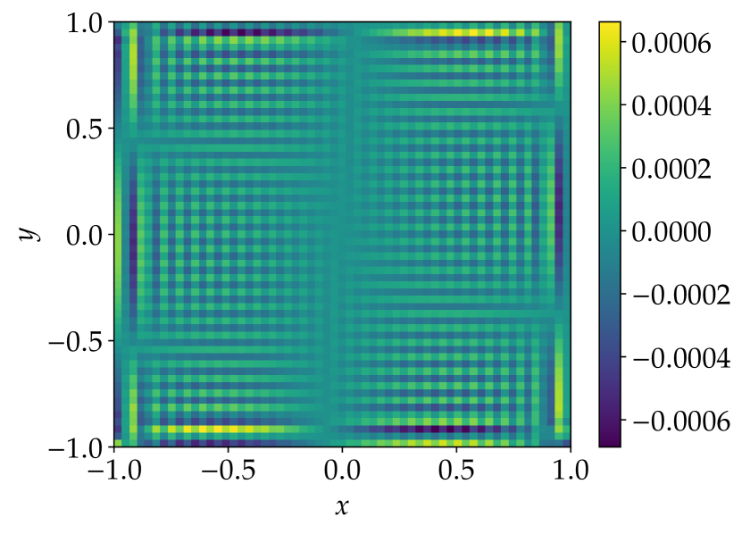
(b) Second component $\boldsymbol{r}_{2}$.

Figure 2: Remainder $\boldsymbol{r}=\boldsymbol{u}-\operatorname{grad}\boldsymbol{\varphi}-\operatorname{rot}\boldsymbol{v}$ of the discrete Helmholtz Hodge decomposition using the sixth order operator of [36] and $N_{1}=N_{2}=60$ grid points per coordinate direction for the problem given by (87).

Because of the scaling by the square root of the mass matrix described in Section 5.1, the discrete projections are (numerically) orthogonal with respect to the scalar product induced by the mass matrix $M$. In this example,

$$\left\langle{\boldsymbol{u}-\operatorname{grad}\boldsymbol{\varphi},\,\operatorname{grad}\boldsymbol{\varphi}}\right\rangle_{M} =$-2.15\text{\times}{10}^{-15}$,$$ (88)

$$\left\langle{\boldsymbol{u}-\operatorname{grad}\boldsymbol{\varphi}-\operatorname{rot}\boldsymbol{v},\,\operatorname{rot}\boldsymbol{v}}\right\rangle_{M} =$9.26\text{\times}{10}^{-15}$.$$

6.2 Convergence Tests in Two Space Dimensions

Using the same setup (87) as in the previous section, convergence tests using the second, fourth, sixth, and eighth order operators of [36] are performed on $N_{1}=N_{2}=N$ nodes per coordinate direction.

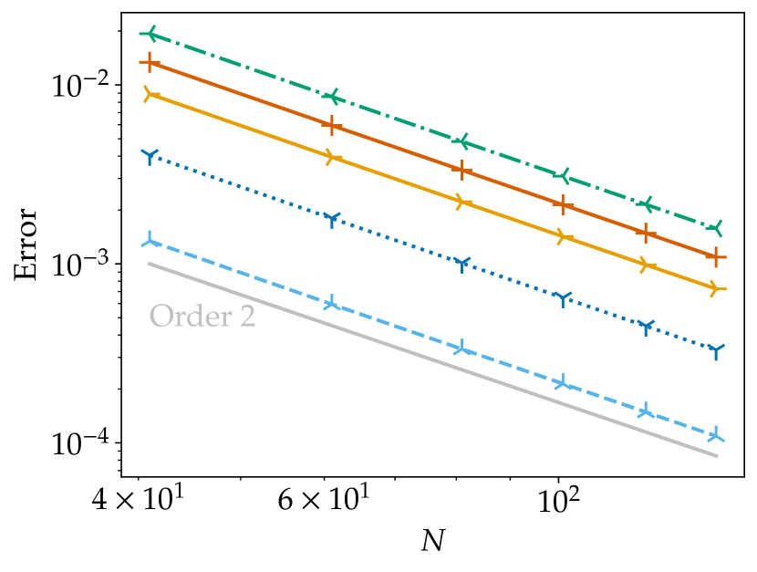
(a) Interior order $2p=2$.

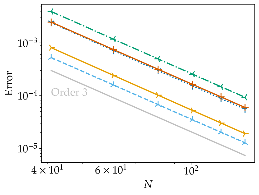
(b) Interior order $2p=4$.

(c) Interior order $2p=6$.

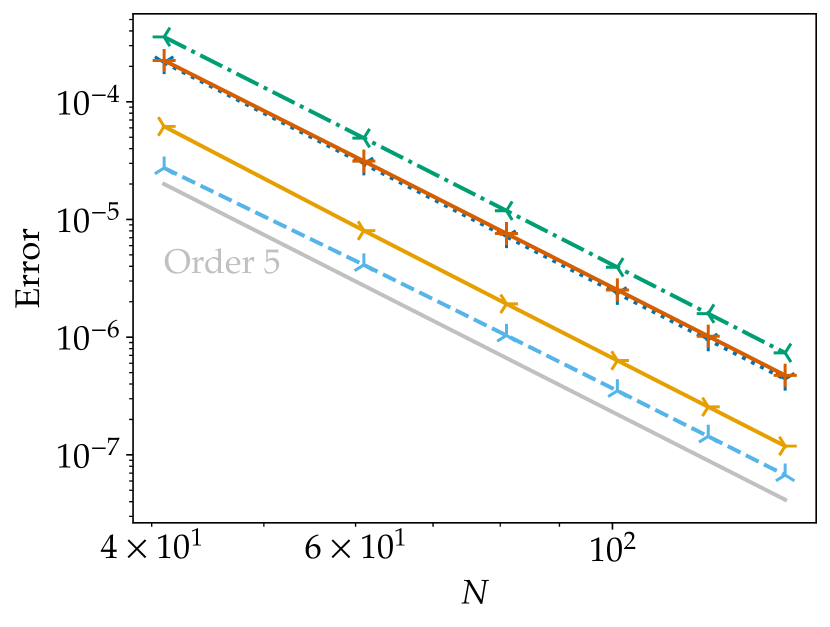
(d) Interior order $2p=8$.

Figure 3: Convergence diagrams of the discrete Helmholtz Hodge decomposition in two space dimensions using the SBP operators of [36] and $N_{1}=N_{2}=N$ grid points per coordinate direction for the problem given by (87).

The results are visualised in Figure 3. Both the potentials $\boldsymbol{\varphi},\boldsymbol{v}$ and the irrotational/solenoidal parts $\operatorname{grad}\boldsymbol{\varphi}=\boldsymbol{u}_{\mathrm{irr}}$, $\operatorname{rot}\boldsymbol{v}=\boldsymbol{u}_{\mathrm{sol}}$ converge with an experimental order of accuracy of $p+1$, as for suitable discretisations of some first order PDEs. The only exception is given by the vector potential $\boldsymbol{v}$ for the operator with interior order of accuracy $2p=6$, which show an experimental order of convergence of $4.6$ instead of $p+1=4$.

6.3 Convergence Tests in Three Space Dimensions

Here, another convergence test in three space dimensions is conducted. The problem is given by

$$\begin{gathered}u(x_{1},x_{2},x_{3})=\operatorname{grad}\varphi+\operatorname{curl}v,\\ \varphi(x_{1},x_{2},x_{3})=\frac{1}{\pi}\sin(\pi x_{1})\sin(\pi x_{2})\sin(\pi x_{3}),\\ v(x_{1},x_{2},x_{3})=\frac{1}{\pi}\begin{pmatrix}\sin(\pi x_{1})\cos(\pi x_{2})\cos(\pi x_{3})\\ \cos(\pi x_{1})\sin(\pi x_{2})\cos(\pi x_{3})\\ -2*\cos(\pi x_{1})\cos(\pi x_{2})\sin(\pi x_{3})\end{pmatrix},\end{gathered}$$ (89)

in the domain $[-1,1]^{3}$. Again, the irrotational part $u_{\mathrm{irr}}=\operatorname{grad}\varphi$ and the solenoidal part $u_{\mathrm{sol}}=\operatorname{curl}v$ can be computed exactly. For this problem, the projection onto $\operatorname{im}\operatorname{curl}$ is performed at first, in accordance with the boundary conditions $\varphi|_{\partial\Omega}=0$ and $v\cdot\nu|_{\partial\Omega}=0$ satisfied by the potentials $\varphi,\psi$, cf. Proposition 5.4. As before, the second, fourth, sixth, and eighth order operators of [36] are applied and $N_{1}=N_{2}=N_{3}=N$ nodes per coordinate direction are used.

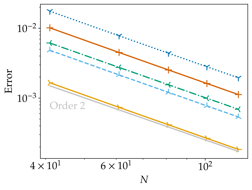
(a) Interior order $2p=2$.

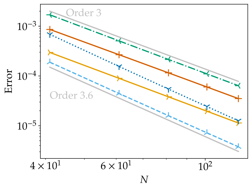
(b) Interior order $2p=4$.

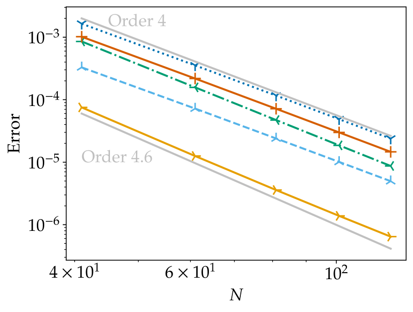
(c) Interior order $2p=6$.

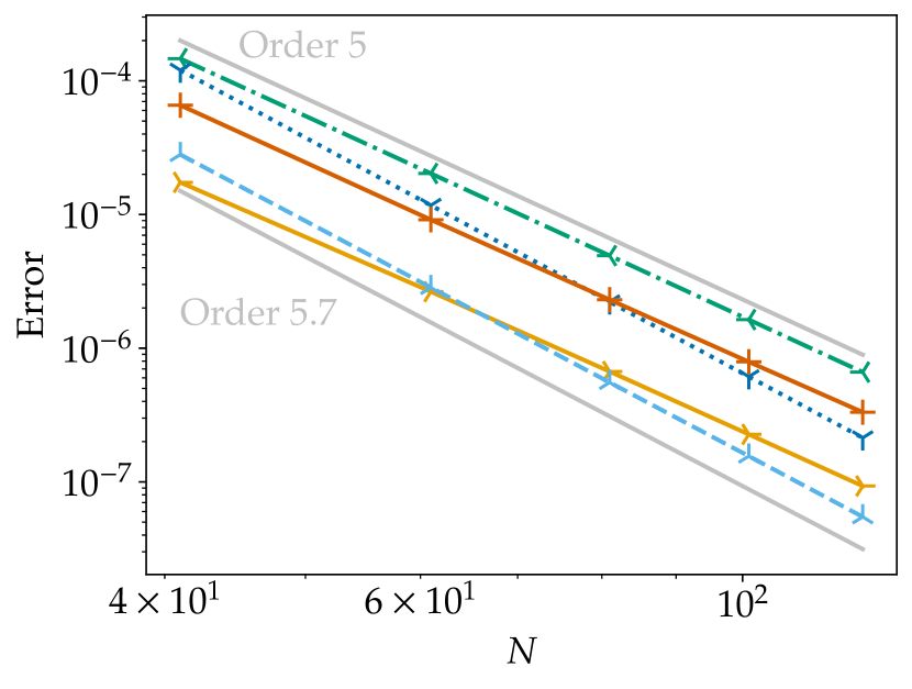
(d) Interior order $2p=8$.

Figure 4: Convergence diagrams of the discrete Helmholtz Hodge decomposition in three space dimensions using the SBP operators of [36] and $N_{1}=N_{2}=N_{3}=N$ grid points per coordinate direction for the problem given by (89).

The results visualised in Figure 4 are similar to the two-dimensional case considered before: The potentials and irrotational/solenoidal components converge at least with an experimental order of accuracy $p+1$ for an SBP operator with interior accuracy $2p$. Some potentials or parts converge with an even higher order $\approx p+1.5$ for the operators with $2p\in\left\{4,6,8\right\}$ in this test case.

6.4 Analysis of MHD Wave Modes

Here, the discrete Helmholtz Hodge decomposition will be applied to analyse linear wave modes in ideal MHD. While the envisioned application in the future concerns the analysis of numerical results obtained using SBP methods, analytical fields will be used here to study the applicability of the methods developed in this article.

Consider a magnetic field

$$B(x_{1},x_{2},x_{3})=\underbrace{\begin{pmatrix}0\\ 0\\ 1\end{pmatrix}}_{\mathllap{\text{background}}}+\underbrace{\begin{pmatrix}0\\ \varepsilon_{A}\sin(k_{1}x_{1}+k_{3}x_{3})\\ 0\end{pmatrix}}_{\mathclap{\text{Alfv\'{e}n}}}+\underbrace{\begin{pmatrix}0\\ 0\\ -\varepsilon_{m}\sin(k_{1}x_{1}+k_{3}x_{3})\end{pmatrix}}_{\mathclap{\text{magnetosonic}}},$$ (90)

given as the sum of a background field, a transversal Alfvén mode, and a longitudinal (fast) magnetosonic mode [50, Chapter 23]. Here, $\varepsilon_{A},\varepsilon_{m}$ are the amplitudes of the linear waves and $k=(k_{1},0,k_{3})$ is the wave vector.

This magnetic field is discretised on a grid using $N_{1}=N_{2}=N_{3}=N$ nodes per coordinate direction in the box $\Omega=[-1,1]^{3}$. The current density $\boldsymbol{j}=\operatorname{curl}\boldsymbol{B}$ is computed discretely and evaluated at the plane given by $x_{3}=0$. There, the first and second component of $\boldsymbol{j}$ form the perpendicular current $\boldsymbol{j}^{\perp}$ in the $x_{1}$-$x_{2}$ plane. In the setup described above, the Alfvén mode is linked to $\boldsymbol{j}^{\perp}_{1}$ and the magnetosonic mode yields $\boldsymbol{j}^{\perp}_{2}$.

Since the magnetosonic current is closed in the plane, the corresponding part of $\boldsymbol{j}^{\perp}$ is divergence free. Since the Alfvén mode yields a current parallel to the background field, the corresponding part of $\boldsymbol{j}^{\perp}$ is not solenoidal but can be obtained via the Helmholtz Hodge decomposition $\boldsymbol{j}^{\perp}=\operatorname{grad}\boldsymbol{\varphi}+\operatorname{rot}\boldsymbol{v}+\boldsymbol{r}$, where $\boldsymbol{r}\neq\boldsymbol{0}$ discretely in general.

While the Helmholtz Hodge decomposition is defined uniquely if $\Omega=\mathbb{R}^{n}$ is considered and can be used in plasma theory, there are some problems in bounded domains because of the boundary effects/conditions. Numerically, discretisation errors will also play a role.

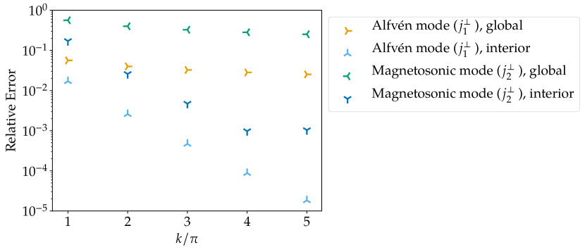
Figure 5: Errors of the wave mode components obtained via the discrete Helmholtz Hodge decomposition (projecting at first onto $\operatorname{im}\operatorname{rot}$) using the sixth order operator of [36] and $N=101$ grid points per coordinate direction with parameters $k_{1}=k_{3}=k$, $\varepsilon_{A}=10^{-3}$, $\varepsilon_{m}=10^{-2}$. The global error is significantly bigger than the one in the interior (measured in the central quarter of the domain) because of disturbances at the boundaries.

The following observations have been made in this setup.

• If one of the amplitudes $\varepsilon_{A},\varepsilon_{m}$ vanishes and the projections are chosen in the correct order (projecting at first onto $\operatorname{im}\operatorname{grad}$ if $\varepsilon_{A}\neq 0$ and onto $\operatorname{im}\operatorname{rot}$ if $\varepsilon_{m}\neq 0$), $\operatorname{grad}\boldsymbol{\varphi}$ reproduces the current density of the Alfvén mode and $\operatorname{rot}\boldsymbol{v}$ that of the magnetosonic mode with only insignificant numerical artefacts.

• If the Alfvén and magnetosonic modes have amplitudes of the same order of magnitude, the order of the projections matters and disturbances are visible at the boundaries. Such disturbances occur even if one of the amplitudes vanishes but the projections are done in the wrong order.

  In Figure 5, errors of the wave mode components obtained via the discrete Helmholtz Hodge decomposition for such a test case are presented. Clearly, the global error is significantly bigger than the one in the interior (a square, centred in the middle of the domain, with one quarter of the total area).

• The disturbances from the boundaries are reduced if more waves are contained in the domain (e.g. if $k_{1},k_{3}$ are increased while keeping the domain $\Omega$ constant). For example, five waves in $\Omega$ have been sufficient in most numerical experiments to yield visually good results in the interior, cf. Figure 5.

• If one of the amplitudes is significantly bigger than the other one, e.g. because of phase mixing, the order of the projections should be chosen to match the order of the amplitudes to get better results. Thus, one should project at first onto $\operatorname{im}\operatorname{grad}$ if $\varepsilon_{A}\gg\varepsilon_{m}$ and at first onto $\operatorname{im}\operatorname{rot}$ if $\varepsilon_{m}\gg\varepsilon_{A}$. Otherwise, the smaller component is dominated by undesired contributions of the other one to its potential.

• If the ratio of the amplitudes is too big, contributions of the dominant mode can pollute the potential for the other mode significantly. The size of ratios that can be resolved on the grid depends on the number of grid nodes (increased resolution increases visible ratios) and the chosen SBP operator. For example, $\varepsilon_{A}=10^{-2}$ and $\varepsilon_{m}=10^{-4}$ yields acceptable results for the sixth order operator using $N=61$ nodes. Choosing instead $\varepsilon_{m}=10^{-5}$, undesired contributions of the Alfvén mode to $(\operatorname{rot}\boldsymbol{v})_{2}$ are an order of magnitude bigger than the desired contributions of the magnetosonic mode. This mode is visible again if the resolution is increased, e.g. to $N=101$ grid points.

To sum up, the order of the projections has to be chosen depending on the given data and one should experiment with both possibilities if there are no clear hints concerning an advantageous choice. Additionally, there should be enough waves in order to yield useful results that are not influenced too much by the boundaries. Finally, the resolution should be high enough if big ratios of the amplitudes are present.

If these conditions are satisfied, the discrete Helmholtz Hodge decomposition can be applied successfully to analyse linear MHD wave modes. A typical plot of the results for a ratio of wave amplitudes of $10^{3}$ is shown in Figure 6.

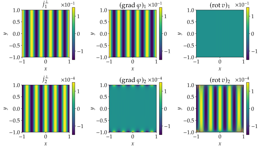
(a) Projecting at first onto $\operatorname{im}\operatorname{grad}$.

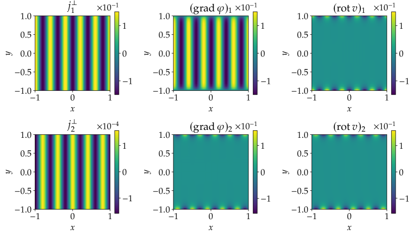
(b) Projecting at first onto $\operatorname{im}\operatorname{rot}$.

Figure 6: Discrete current density $\boldsymbol{j}^{\perp}$ and its Helmholtz Hodge decomposition using the sixth order operator of [36] and $N=101$ grid points per coordinate direction with parameters $k_{1}=k_{3}=5\pi$, $\varepsilon_{A}=10^{-2}$, $\varepsilon_{m}=10^{-5}$.

Characterising the chosen variant of the Helmholtz Hodge decomposition using boundary conditions is not necessarily advantageous in this example. Indeed, the ratio of the amplitudes of the Alfvén and magnetosonic waves does not influence the different types of homogeneous boundary conditions given in Propositions 5.3 and 5.4 (as long as both amplitudes $\varepsilon_{A}$ and $\varepsilon_{m}$ do not vanish). Hence, basing a choice of a variant of the Helmholtz Hodge decomposition solely on boundary conditions, one would not expect to see a qualitative difference between the behaviour of the variants for $\varepsilon_{A}\gg\varepsilon_{m}$ vs. $\varepsilon_{A}\ll\varepsilon_{m}$. However, such a qualitative difference can be clearly observed in practice, as can be seen by comparing Figure 6 ($\varepsilon_{A}\gg\varepsilon_{m}$) to Figure 7 ($\varepsilon_{A}\ll\varepsilon_{m}$). In the former case, projecting at first onto $\operatorname{im}\operatorname{grad}$ is advantageous while projecting at first onto $\operatorname{im}\operatorname{rot}$ is better in the latter case. This behaviour is in accordance with the discussion above based on the interpretation of the variants of the Helmholtz Hodge decomposition as projections using different orders.

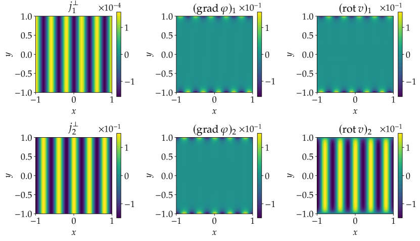
(a) Projecting at first onto $\operatorname{im}\operatorname{grad}$.

(b) Projecting at first onto $\operatorname{im}\operatorname{rot}$.

Figure 7: Discrete current density $\boldsymbol{j}^{\perp}$ and its Helmholtz Hodge decomposition using the sixth order operator of [36] and $N=101$ grid points per coordinate direction with parameters $k_{1}=k_{3}=5\pi$, $\varepsilon_{A}=10^{-5}$, $\varepsilon_{m}=10^{-2}$.

7 Summary and Discussion

In this article, discrete variants of classical results from vector calculus for finite difference summation by parts operators have been investigated. Firstly, it has been proven that discrete variants of the classical existence theorems for scalar/vector potentials of curl/divergence free vector fields cannot hold discretely, cf. Theorems 3.7, 3.8, 3.18, and 3.19, basically because of the finite dimensionality of the discrete functions spaces and the presence of certain types of grid oscillations.

Based on these results, it has been shown that discrete Helmholtz Hodge decompositions $\boldsymbol{u}=\operatorname{grad}\boldsymbol{\varphi}+\operatorname{curl}\boldsymbol{v}+\boldsymbol{r}$ of a given vector field $\boldsymbol{u}$ into an irrotational component $\boldsymbol{u}_{\mathrm{irr}}=\operatorname{grad}\boldsymbol{\varphi}$ and a solenoidal part $\boldsymbol{u}_{\mathrm{sol}}=\operatorname{curl}\boldsymbol{v}$ will in general have a non-vanishing remainder $\boldsymbol{r}$, contrary to the continuous case, cf. Section 5. This remainder $\boldsymbol{r}\neq\boldsymbol{0}$ is associated to certain types of grid oscillations, as supported by theoretical insights and numerical experiments in Section 6. There, applications to the analysis of MHD wave modes are presented and discussed additionally.

Classically, different variants of the Helmholtz Hodge decomposition in bounded domains are most often presented with an emphasis on boundary conditions. Taking another point of view, these variants can also be interpreted as results of two orthogonal projections in a Hilbert space, i.e. as least squares problems. Since the images/ranges of these projections are not orthogonal, the projections do not commute and their order matters, resulting in different variants of the decomposition. At the continuous level, these correspond to the different types of boundary/secondary conditions for the potentials in the associated normal equations of the least squares problems, which are elliptic PDEs. Here, computing the least norm least squares solution via iterative methods has been proposed and applied successfully to compute discrete Helmholtz Hodge decompositions. Using advanced iterative solvers such as LSQR or LSMR, the solution of the least norm least squares problem for the projections corresponds to the solution of the underlying elliptic PDEs via the related iterative methods, e.g. CG for LSQR and MINRES for LSMR. However, LSQR/LSMR are known to have some advantageous properties compared to the application of CG/MINRES to the discretised elliptic PDEs.

The basic argument for the impossibility of a discrete Poincaré lemma (existence of scalar/vector potentials for irrotational/solenoidal vector fields) uses the finite dimension of the discrete function spaces and the collocation approach. If staggered grids are used instead, these arguments do not hold in the same form and potentials exist for some (low order) operators, e.g. in [52] or for the mimetic operators of [26]. Hence, it will be interesting to consider staggered grid SBP operators in this context, cf. [40, 37, 16].

At the continuous level, there are two widespread versions of the Helmholtz Hodge decomposition, characterised either by the choice of boundary conditions for the potentials or by the order of projections onto $\operatorname{im}\operatorname{grad}=\operatorname{ker}\operatorname{curl}$ and $\operatorname{im}\operatorname{curl}=\operatorname{ker}\operatorname{div}$. Since there are different possibilities to impose boundary conditions and the relations of the images and kernels do not hold discretely, there are several other discrete variants. In this article, orthogonal projections onto $\operatorname{im}\operatorname{grad}$ and $\operatorname{im}\operatorname{curl}$ have been considered, corresponding to a certain weak imposition of boundary conditions for the potentials. Projecting instead onto $\operatorname{ker}\operatorname{curl}$ and $\operatorname{ker}\operatorname{div}$ is another option that seems to be viable and will be studied in the future.

The iterative methods used for the orthogonal projections in this article are equivalent to the application of certain methods such as CG or MINRES to the associated discrete normal equations in exact arithmetic. At the continuous level, these normal equations are elliptic second order problems. For example, the scalar potential is associated to a Neumann problem. These elliptic PDEs could also be solved discretely using (compatible) narrow stencil operators while the discrete normal problems are associated to wide stencil operators. There are also other approaches to approximate Helmholtz Hodge decompositions discretely, e.g. [4, 2]. While a detailed comparison of all these approaches is out of the scope of this article, it would be interesting for the community and physicists interested in the application of discrete Helmholtz Hodge decompositions. Of course, the advantages and drawbacks of different iterative solvers and preconditioners should be considered for such a detailed comparison as well.

References

- [1] Etienne Ahusborde, Mejdi Azaiez and Jean-Paul Caltagirone “A primal formulation for the Helmholtz decomposition” In Journal of Computational Physics 225.1 Elsevier, 2007, pp. 13–19 DOI: 10.1016/j.jcp.2007.04.002
- [2] Etienne Ahusborde et al. “Discrete Hodge Helmholtz Decomposition” In Monografías Matemáticas García de Galdeano 39, 2014, pp. 1–10
- [3] Cherif Amrouche, Christine Bernardi, Monique Dauge and Vivette Girault “Vector potentials in three-dimensional non-smooth domains” In Mathematical Methods in the Applied Sciences 21.9 Wiley Online Library, 1998, pp. 823–864 DOI: 10.1002/(SICI)1099-1476(199806)21:9<823::AID-MMA976>3.0.CO;2-B
- [4] Philippe Angot, Jean-Paul Caltagirone and Pierre Fabrie “Fast discrete Helmholtz–Hodge decompositions in bounded domains” In Applied Mathematics Letters 26.4 Elsevier, 2013, pp. 445–451 DOI: 10.1016/j.aml.2012.11.006
- [5] Andrey Beresnyak and Alexander Lazarian “Turbulence in magnetohydrodynamics” 12, Studies in Mathematical Physics Walter de Gruyter GmbH & Co KG, 2019
- [6] Jeff Bezanson, Alan Edelman, Stefan Karpinski and Viral B Shah “Julia: A Fresh Approach to Numerical Computing” In SIAM Review 59.1 SIAM, 2017, pp. 65–98 DOI: 10.1137/141000671
- [7] Harsh Bhatia, Gregory Norgard, Valerio Pascucci and Peer-Timo Bremer “The Helmholtz-Hodge decomposition — A Survey” In IEEE Transactions on Visualization and Computer Graphics 19.8 IEEE, 2012, pp. 1386–1404 DOI: 10.1109/TVCG.2012.316
- [8] Jesse Chan “On discretely entropy conservative and entropy stable discontinuous Galerkin methods” In Journal of Computational Physics 362 Elsevier, 2018, pp. 346–374 DOI: 10.1016/j.jcp.2018.02.033
- [9] Ron Estrin, Dominique Orban and Michael A Saunders “LSLQ: An Iterative Method for Linear Least-Squares with an Error Minimization Property” In SIAM Journal on Matrix Analysis and Applications 40.1 SIAM, 2019, pp. 254–275 DOI: 10.1137/17M1113552
- [10] Paolo Fernandes and Gianni Gilardi “Magnetostatic and electrostatic problems in inhomogeneous anisotropic media with irregular boundary and mixed boundary conditions” In Mathematical Models and Methods in Applied Sciences 7.07 World Scientific, 1997, pp. 957–991 DOI: 10.1142/S0218202597000487
- [11] David C Del Rey Fernández, Pieter D Boom, Mark H Carpenter and David W Zingg “Extension of Tensor-Product Generalized and Dense-Norm Summation-by-Parts Operators to Curvilinear Coordinates” In Journal of Scientific Computing Springer, pp. 1–40 DOI: 10.1007/s10915-019-01011-3
- [12] David C Del Rey Fernández, Pieter D Boom and David W Zingg “A generalized framework for nodal first derivative summation-by-parts operators” In Journal of Computational Physics 266 Elsevier, 2014, pp. 214–239 DOI: 10.1016/j.jcp.2014.01.038
- [13] David C Del Rey Fernández, Jason E Hicken and David W Zingg “Review of summation-by-parts operators with simultaneous approximation terms for the numerical solution of partial differential equations” In Computers & Fluids 95 Elsevier, 2014, pp. 171–196 DOI: 10.1016/j.compfluid.2014.02.016
- [14] Travis C Fisher and Mark H Carpenter “High-order entropy stable finite difference schemes for nonlinear conservation laws: Finite domains” In Journal of Computational Physics 252 Elsevier, 2013, pp. 518–557 DOI: 10.1016/j.jcp.2013.06.014
- [15] David Chin-Lung Fong and Michael A Saunders “LSMR: An Iterative Algorithm for Sparse Least-Squares Problems” In SIAM Journal on Scientific Computing 33.5 SIAM, 2011, pp. 2950–2971 DOI: 10.1137/10079687X
- [16] Longfei Gao, David C Del Rey Fernández, Mark Carpenter and David Keyes “SBP–SAT finite difference discretization of acoustic wave equations on staggered block-wise uniform grids” In Journal of Computational and Applied Mathematics 348 Elsevier, 2019, pp. 421–444 DOI: 10.1016/j.cam.2018.08.040
- [17] Gregor J Gassner “A Skew-Symmetric Discontinuous Galerkin Spectral Element Discretization and Its Relation to SBP-SAT Finite Difference Methods” In SIAM Journal on Scientific Computing 35.3 Society for IndustrialApplied Mathematics, 2013, pp. A1233–A1253 DOI: 10.1137/120890144
- [18] Vivette Girault and Pierre-Arnaud Raviart “Finite Element Methods for Navier-Stokes Equations: Theory and Algorithms” 5, Springer Series in Computational Mathematics Berlin Heidelberg: Springer Science & Business Media, 2012 DOI: 10.1007/978-3-642-61623-5
- [19] Karl-Heinz Glaßmeier “Reconstruction of the ionospheric influence on ground-based observations of a short-duration ULF pulsation event” In Planetary and Space Science 36.8 Elsevier, 1988, pp. 801–817 DOI: 10.1016/0032-0633(88)90086-4
- [20] Karl-Heinz Glaßmeier “Reflection of MHD-waves in the Pc4-5 period range at ionospheres with non-uniform conductivity distributions” In Geophysical Research Letters 10.8 Wiley Online Library, 1983, pp. 678–681 DOI: 10.1029/GL010i008p00678
- [21] Karl-Heinz Glaßmeier et al. “Magnetospheric Field Line Resonances: A Comparative Planetology Approach” In Surveys in Geophysics 20.1 Springer, 1999, pp. 61–109 DOI: 10.1023/A:1006659717963
- [22] K-H Glaßmeier “On the influence of ionospheres with non-uniform conductivity distribution on hydromagnetic waves” In Journal of Geophysics 54, 1984, pp. 125–137
- [23] Jason E Hicken and David W Zingg “Summation-by-parts operators and high-order quadrature” In Journal of Computational and Applied Mathematics 237.1 Elsevier, 2013, pp. 111–125 DOI: 10.1016/j.cam.2012.07.015
- [24] H.. Huynh “A Flux Reconstruction Approach to High-Order Schemes Including Discontinuous Galerkin Methods” In 18th AIAA Computational Fluid Dynamics Conference, 2007 American Institute of AeronauticsAstronautics DOI: 10.2514/6.2007-4079
- [25] James M Hyman and Mikhail Shashkov “Natural discretizations for the divergence, gradient, and curl on logically rectangular grids” In Computers & Mathematics with Applications 33.4 Elsevier, 1997, pp. 81–104 DOI: 10.1016/S0898-1221(97)00009-6
- [26] James M Hyman and Mikhail Shashkov “The orthogonal decomposition theorems for mimetic finite difference methods” In SIAM Journal on Numerical Analysis 36.3 SIAM, 1999, pp. 788–818 DOI: 10.1137/S0036142996314044
- [27] Vasilii Vasil’evich Jikov, Sergei M Kozlov and Olga Arsen’evna Oleinik “Homogenization of Differential Operators and Integral Functionals” Berlin Heidelberg: Springer Science & Business Media, 1994 DOI: 10.1007/978-3-642-84659-5
- [28] Grzegorz Kowal and Alex Lazarian “Velocity field of compressible magnetohydrodynamic turbulence: wavelet decomposition and mode scalings” In The Astrophysical Journal 720.1 IOP Publishing, 2010, pp. 742 DOI: 10.1088/0004-637X/720/1/742
- [29] Heinz-Otto Kreiss and Godela Scherer “Finite Element and Finite Difference Methods for Hyperbolic Partial Differential Equations” In Mathematical Aspects of Finite Elements in Partial Differential Equations New York: Academic Press, 1974, pp. 195–212
- [30] Antoine Lemoine, J-P Caltagirone, Mejdi Azaïez and Stéphane Vincent “Discrete Helmholtz–Hodge decomposition on polyhedral meshes using compatible discrete operators” In Journal of Scientific Computing 65.1 Springer, 2015, pp. 34–53 DOI: 10.1007/s10915-014-9952-8
- [31] Viktor Linders, Tomas Lundquist and Jan Nordström “On the order of Accuracy of Finite Difference Operators on Diagonal Norm Based Summation-By-Parts Form” In SIAM Journal on Numerical Analysis 56.2 SIAM, 2018, pp. 1048–1063 DOI: 10.1137/17M1139333
- [32] Viktor Linders, Jan Nordström and Steven H Frankel “Convergence and stability properties of summation-by-parts in time” Linköping, Sweden: Linköping University Electronic Press, 2019
- [33] Konstantin Lipnikov, Gianmarco Manzini and Mikhail Shashkov “Mimetic finite difference method” In Journal of Computational Physics 257 Elsevier, 2014, pp. 1163–1227 DOI: 10.1016/j.jcp.2013.07.031
- [34] Ken Mattsson, Martin Almquist and Mark H Carpenter “Optimal diagonal-norm SBP operators” In Journal of Computational Physics 264 Elsevier, 2014, pp. 91–111 DOI: 10.1016/j.jcp.2013.12.041
- [35] Ken Mattsson, Martin Almquist and Edwin Weide “Boundary optimized diagonal-norm SBP operators” In Journal of computational physics 374 Elsevier, 2018, pp. 1261–1266 DOI: 10.1016/j.jcp.2018.06.010
- [36] Ken Mattsson and Jan Nordström “Summation by parts operators for finite difference approximations of second derivatives” In Journal of Computational Physics 199.2 Elsevier, 2004, pp. 503–540 DOI: 10.1016/j.jcp.2004.03.001
- [37] Ken Mattsson and Ossian O’Reilly “Compatible diagonal-norm staggered and upwind SBP operators” In Journal of Computational Physics 352 Elsevier, 2018, pp. 52–75 DOI: 10.1016/j.jcp.2017.09.044
- [38] Jan Nordström and Martin Björck “Finite volume approximations and strict stability for hyperbolic problems” In Applied Numerical Mathematics 38.3 Elsevier, 2001, pp. 237–255 DOI: 10.1016/S0168-9274(01)00027-7
- [39] Jan Nordström, Karl Forsberg, Carl Adamsson and Peter Eliasson “Finite volume methods, unstructured meshes and strict stability for hyperbolic problems” In Applied Numerical Mathematics 45.4 Elsevier, 2003, pp. 453–473 DOI: 10.1016/S0168-9274(02)00239-8
- [40] Ossian O’Reilly, Tomas Lundquist, Eric M Dunham and Jan Nordström “Energy stable and high-order-accurate finite difference methods on staggered grids” In Journal of Computational Physics 346 Elsevier, 2017, pp. 572–589 DOI: 10.1016/j.jcp.2017.06.030
- [41] Christopher C Paige and Michael A Saunders “Algorithm 583 LSQR: Sparse Linear Equations and Least Squares Problems” In ACM Transactions on Mathematical Software (TOMS) 8.2 ACM, 1982, pp. 195–209 DOI: 10.1145/355993.356000
- [42] Christopher C Paige and Michael A Saunders “LSQR: An Algorithm for Sparse Linear Equations and Sparse Least Squares” In ACM Transactions on Mathematical Software (TOMS) 8.1 ACM, 1982, pp. 43–71 DOI: 10.1145/355984.355989
- [43] Hendrik Ranocha “Mimetic Properties of Difference Operators: Product and Chain Rules as for Functions of Bounded Variation and Entropy Stability of Second Derivatives” In BIT Numerical Mathematics 59.2 Springer, 2019, pp. 547–563 DOI: 10.1007/s10543-018-0736-7
- [44] Hendrik Ranocha “Shallow water equations: Split-form, entropy stable, well-balanced, and positivity preserving numerical methods” In GEM – International Journal on Geomathematics 8.1, 2017, pp. 85–133 DOI: 10.1007/s13137-016-0089-9
- [45] Hendrik Ranocha “Some Notes on Summation by Parts Time Integration Methods” In Results in Applied Mathematics 1 Elsevier, 2019, pp. 100004 DOI: 10.1016/j.rinam.2019.100004
- [46] Hendrik Ranocha, Philipp Öffner and Thomas Sonar “Extended skew-symmetric form for summation-by-parts operators and varying Jacobians” In Journal of Computational Physics 342 Elsevier, 2017, pp. 13–28 DOI: 10.1016/j.jcp.2017.04.044
- [47] Hendrik Ranocha, Philipp Öffner and Thomas Sonar “Summation-by-parts operators for correction procedure via reconstruction” In Journal of Computational Physics 311 Elsevier, 2016, pp. 299–328 DOI: 10.1016/j.jcp.2016.02.009
- [48] Hendrik Ranocha, Katharina Ostaszewski and Philip Heinisch “2019_SBP_vector_calculus_REPRO. Discrete Vector Calculus and Helmholtz Hodge Decomposition for Classical Finite Difference Summation by Parts Operators”, https://github.com/IANW-Projects/2019_SBP_vector_calculus_REPRO, 2019 DOI: 10.5281/zenodo.3375170
- [49] Hendrik Ranocha, Katharina Ostaszewski and Philip Heinisch “Numerical Methods for the Magnetic Induction Equation with Hall Effect and Projections onto Divergence-Free Vector Fields” Submitted, 2018 arXiv:1810.01397 [math.NA]
- [50] Dalton D. Schnack “Lectures in Magnetohydrodynamics With an Appendix on Extended MHD” Berlin Heidelberg: Springer, 2009 DOI: 10.1007/978-3-642-00688-3
- [51] Ben Schweizer “On Friedrichs inequality, Helmholtz decomposition, vector potentials, and the div-curl lemma” In Trends in Applications of Mathematics to Mechanics 27, Springer INdAM Series Cham: Springer, 2018, pp. 65–79 DOI: 10.1007/978-3-319-75940-1_4
- [52] Zachary J Silberman et al. “Numerical generation of vector potentials from specified magnetic fields” In Journal of Computational Physics 379 Elsevier, 2019, pp. 421–437 DOI: 10.1016/j.jcp.2018.12.006
- [53] J.A. Sims et al. “Directional analysis of cardiac motion field from gated fluorodeoxyglucose PET images using the Discrete Helmholtz Hodge Decomposition” In Computerized Medical Imaging and Graphics 65 Elsevier, 2018, pp. 69–78 DOI: 10.1016/j.compmedimag.2017.06.004
- [54] Björn Sjögreen, Helen C Yee and Dmitry Kotov “Skew-symmetric splitting and stability of high order central schemes” In Journal of Physics: Conference Series 837.1, 2017, pp. 012019 IOP Publishing DOI: 10.1088/1742-6596/837/1/012019
- [55] Bo Strand “Summation by Parts for Finite Difference Approximations for ” In Journal of Computational Physics 110.1 Elsevier, 1994, pp. 47–67 DOI: 10.1006/jcph.1994.1005
- [56] Magnus Svärd “A note on bounds and convergence rates of summation-by-parts schemes” In BIT Numerical Mathematics 54.3 Springer, 2014, pp. 823–830 DOI: 10.1007/s10543-014-0471-7
- [57] Magnus Svärd “On Coordinate Transformations for Summation-by-Parts Operators” In Journal of Scientific Computing 20.1 Springer, 2004, pp. 29–42 DOI: 10.1023/A:1025881528802
- [58] Magnus Svärd and Jan Nordström “On the convergence rates of energy-stable finite-difference schemes” Linköping, Sweden: Linköping University Electronic Press, 2017
- [59] Magnus Svärd and Jan Nordström “On the order of accuracy for difference approximations of initial-boundary value problems” In Journal of Computational Physics 218.1 Elsevier, 2006, pp. 333–352 DOI: 10.1016/j.jcp.2006.02.014
- [60] Magnus Svärd and Jan Nordström “Review of summation-by-parts schemes for initial-boundary-value problems” In Journal of Computational Physics 268 Elsevier, 2014, pp. 17–38 DOI: 10.1016/j.jcp.2014.02.031