Masur-Veech volumes, frequencies of simple closed geodesics and intersection numbers of moduli spaces of curves

Abstract.

We express the Masur–Veech volume $\operatorname{Vol}\mathcal{Q}_{g,n}$ and the area Siegel–Veech constant $c_{\mathit{area}}(\mathcal{Q}_{g,n})$ of the moduli space $\mathcal{Q}_{g,n}$ of meromorphic quadratic differential with $n$ simple poles and no other poles as polynomials in the intersection numbers of $\psi$-classes supported on the boundary cycles of the Deligne–Mumford compactification $\overline{\mathcal{M}}_{g,n}$. The formulae obtained in this article are derived from lattice point count involving the Kontsevich volume polynomials $N_{g,n}(b_{1},\ldots,b_{n})$ that also appear in Mirzakhani’s recursion for the Weil–Petersson volumes of the moduli space $\mathcal{M}_{g,n}(b_{1},\dots,b_{n})$ of bordered hyperbolic Riemann surfaces.

A similar formula for the Masur–Veech volume $\operatorname{Vol}\mathcal{Q}_{g}$ (though without explicit evaluation) was obtained earlier by M. Mirzakhani through completely different approach. We prove further result: up to a normalization factor depending only on $g$ and $n$ (which we compute explicitly), the density of the orbit $\operatorname{Mod}_{g,n}\cdot\gamma$ of any simple closed multicurve $\gamma$ inside the ambient set $\mathcal{ML}_{g,n}({\mathbb{Z}})$ of integral measured laminations computed by Mirzakhani, coincides with the density of square-tiled surfaces having horizontal cylinder decomposition associated to $\gamma$ among all square-tiled surfaces in $\mathcal{Q}_{g,n}$.

We study the resulting densities (or, equivalently, volume contributions) in more detail in the special case when $n=0$. In particular, we compute explicitly the asymptotic frequencies of separating and non-separating simple closed geodesics on a closed hyperbolic surface of genus $g$ for all small genera $g$ and we show that in large genera the separating closed geodesics are $\sqrt{\frac{2}{3\pi g}}\cdot\frac{1}{4^{g}}$ times less frequent.

We conclude with detailed conjectural description of combinatorial geometry of a random simple closed multicurve on a surface of large genus and of a random square-tiled surface of large genus. This description is conditional to the conjectural asymptotic formula for the Masur–Veech volume $\operatorname{Vol}\mathcal{Q}_{g}$ in large genera and to the conjectural uniform asymptotic formula for certain sums of intersection numbers of $\psi$-classes in large genera.

1. Introduction and statements of main theorems

1.1. Masur–Veech volume of the moduli space of quadratic differentials

Consider the moduli space $\mathcal{M}_{g,n}$ of complex curves of genus $g$ with $n$ distinct labeled marked points. The total space $\mathcal{Q}_{g,n}$ of the cotangent bundle over $\mathcal{M}_{g,n}$ can be identified with the moduli space of pairs $(C,q)$, where $C\in\mathcal{M}_{g,n}$ is a smooth complex curve and $q$ is a meromorphic quadratic differential on $C$ with simple poles at the marked points and no other poles. (In the case $n=0$ the quadratic differential $q$ is holomorphic.) Thus, the moduli space of quadratic differentials $\mathcal{Q}_{g,n}$ is endowed with the canonical symplectic structure. The induced volume element $d\!\operatorname{Vol}$ on $\mathcal{Q}_{g,n}$ is called the Masur–Veech volume element. (In Section 2.1 we provide alternative more common definition of the Masur–Veech volume element and explain why two definitions are equivalent.)

A meromorphic quadratic differential $q$ defines a flat metric $|q|$ on the complex curve $C$. The resulting metric has conical singularities at zeroes and simple poles of $q$. When all poles of $q$ (if any) are simple, and when $C$ is a smooth compact curve, the resulting total flat area

$$\operatorname{Area}(C,q)=\int_{C}|q|$$

is finite; it is strictly positive as soon as $q$ is not identically zero. Consider the following subsets in $\mathcal{Q}_{g,n}$:

(1.1) $$\mathcal{Q}^{\operatorname{Area}\leq\frac{1}{2}}_{g,n} =\left\{(C,q)\in\mathcal{Q}_{g,n}\,|\,\operatorname{Area}(C,q)\leq\tfrac{1}{2}\right\}\,,$$

(1.2) $$\mathcal{Q}^{\operatorname{Area}=\frac{1}{2}}_{g,n} =\left\{(C,q)\in\mathcal{Q}_{g,n}\,|\,\operatorname{Area}(C,q)=\tfrac{1}{2}\right\}\,.$$

These subsets might be seen as analogs of a “ball (respectively a sphere) of radius $\tfrac{1}{2}$” in $\mathcal{Q}_{g,n}$. However, this analogy is not quite adequate since none of these two subsets is compact. By the independent results of H. Masur [Ma1] and W. Veech [Ve1], the volume $\operatorname{Vol}\mathcal{Q}^{\operatorname{Area}\leq\frac{1}{2}}_{g,n}$ is finite.

The Masur–Veech volume element $d\!\operatorname{Vol}$ in $\mathcal{Q}_{g,n}$ induces the canonical volume element $d\!\operatorname{Vol}_{1}$ on any noncritical level hypersurface of any real-valued function $f$. In particular, it induces the canonical volume element $d\!\operatorname{Vol}_{1}$ on the level hypersurface $\mathcal{Q}^{\operatorname{Area}=\frac{1}{2}}_{g,n}$ satisfying

(1.3) $$\operatorname{Vol}_{1}\mathcal{Q}^{\operatorname{Area}=\frac{1}{2}}_{g,n}=(12g-12+4n)\cdot\operatorname{Vol}\mathcal{Q}^{\operatorname{Area}\leq\frac{1}{2}}_{g,n}\,.$$

Here $12g-12+4n=\dim_{{\mathbb{R}}}\mathcal{Q}_{g,n}=2\dim_{{\mathbb{C}}}\mathcal{Q}_{g,n}$. The above formula can be considered as the definition of the expression on the left hand side.

Convention 1.1.

The Masur–Veech volume of the total space $\mathcal{Q}_{g,n}$ is, clearly, infinite. Following the common convention, speaking of the Masur–Veech volume of the moduli space $\mathcal{Q}_{g,n}$ we always mean the quantity (1.3) and we use the abbreviated notation $\operatorname{Vol}\mathcal{Q}_{g,n}$ for this quantity.

Remark 1.2.

The choice of “radius $\tfrac{1}{2}$” instead of “radius $1$” in (1.3) might seem unexpected. We explain the reasons for this choice in Section 2.1 where we discuss the Masur–Veech volume element in more details. Further details on natural normalizations of the Masur–Veech volume can be found in appendix A in [DGZZ2].

1.2. Square-tiled surfaces, simple closed multicurves and stable graphs

We have already mentioned that a meromorphic quadratic differential $q$ defines a flat metric with conical singularities on the complex curve $C$. One can construct this kind of flat surfaces by assembling together identical polarized oriented flat squares. Namely, we assume that we know which pair of opposite sides of each square is horizontal; the remaining pair of sides is vertical. Gluing the squares we identify sides to sides respecting the polarization and the orientation.

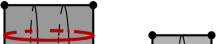
Figure 1. Square-tiled surface in $\mathcal{Q}_{0,7}$, and associated multicurve and stable graph

Suppose that the resulting closed square-tiled surface has genus $g$ and $n$ conical singularities with angle $\pi$, i.e. $n$ vertices adjacent to only two squares. For example, the square-tiled surfaces in Figure 1 has genus $g=0$ and $n=7$ conical singularities with angle $\pi$. Consider the complex coordinate $z$ in each square and a quadratic differential $(dz)^{2}$. It is easy to check that the resulting square-tiled surface inherits the complex structure and globally defined meromorphic quadratic differential $q$ having simple poles at $n$ conical singularities with angle $\pi$ and no other poles. Thus, any square-tiled surface of genus $g$ having $n$ conical singularities with angle $\pi$ canonically defines a point $(C,q)\in\mathcal{Q}_{g,n}$. Fixing the size of the square once and forever and considering all resulting square-tiled surfaces in $\mathcal{Q}_{g,n}$ we get a discrete subset $\mathcal{ST}{}_{g,n}$ in $\mathcal{Q}_{g,n}$.

Define $\mathcal{ST}{}_{g,n}(N)\subset\mathcal{ST}{}_{g,n}$ to be the subset of square-tiled surfaces in $\mathcal{Q}_{g,n}$ tiled with at most $N$ identical squares. We shall see in Section 2.1 that square-tiled surfaces form a lattice in period coordinates of $\mathcal{Q}_{g,n}$, which justifies the following alternative definition of the Masur–Veech volume:

(1.4) $$\operatorname{Vol}\mathcal{Q}_{g,n}=2(6g-6+2n)\cdot\lim_{N\to+\infty}\frac{\operatorname{card}(\mathcal{ST}{}_{g,n}(2N))}{N^{d}}\,,$$

where $d=6g-6+2n=\dim_{{\mathbb{C}}}\mathcal{Q}_{g,n}$. In this formula we assume that all conical singularities of square-tiled surfaces are labeled.

Multicurve associated to a cylinder decomposition. Any square-tiled surface admits a decomposition into maximal horizontal cylinders filled with isometric closed regular flat geodesics. Every such maximal horizontal cylinder has at least one conical singularity on each of the two boundary components. The square-tiled surface in Figure 1 has four maximal horizontal cylinders which are represented in the picture by different shades. For every maximal horizontal cylinder choose the corresponding waist curve $\gamma_{i}$.

By construction each resulting simple closed curve $\gamma_{i}$ is nonperiferal (i.e. it does not bound a topological disc without punctures or with a single puncture) and different $\gamma_{i},\gamma_{j}$ are not freely homotopic on the underlying $n$-punctured topological surface. In other words, pinching simultaneously all waist curves $\gamma_{i}$ we get a legal stable curve in the Deligne–Mumford compactification $\overline{\mathcal{M}}_{g,n}$.

We encode the number of circular horizontal bands of squares contained in the corresponding maximal horizontal cylinder by the integer weight $H_{i}$ associated to the curve $\gamma_{i}$. The above observation implies that the resulting formal linear combination $\gamma=\sum H_{i}\gamma_{i}$ is a simple closed integral multicurve in the space $\mathcal{ML}_{g,n}({\mathbb{Z}})$ of measured laminations. For example, the simple closed multicurve associated to the square-tiled surface as in Figure 1 has the form $2\gamma_{1}+\gamma_{2}+\gamma_{3}+2\gamma_{4}$.

Given a simple closed integral multicurve $\gamma$ in $\mathcal{ML}_{g,n}({\mathbb{Z}})$ consider the subset $\mathcal{ST}{}_{g,n}(\gamma)\subset\mathcal{ST}{}_{g,n}$ of those square-tiled surfaces, for which the associated horizontal multicurve is in the same $\operatorname{Mod}_{g,n}$-orbit as $\gamma$ (i.e. it is homeomorphic to $\gamma$ by a homeomorphism sending $n$ marked points to $n$ marked points and preserving their labeling). Denote by $\operatorname{Vol}(\gamma)$ the contribution to $\operatorname{Vol}\mathcal{Q}_{g,n}$ of square-tiled surfaces from the subset $\mathcal{ST}{}_{g,n}(\gamma)\subset\mathcal{ST}{}_{g,n}$:

$$\operatorname{Vol}(\gamma)=2(6g-6+2n)\cdot\lim_{N\to+\infty}\frac{\operatorname{card}(\mathcal{ST}{}_{g,n}(2N)\cap\mathcal{ST}{}_{g,n}(\gamma))}{N^{d}}\,.$$

The results in [DGZZ2] imply that for any $\gamma$ in $\mathcal{ML}_{g,n}({\mathbb{Z}})$ the above limit exists, is strictly positive, and that

(1.5) $$\operatorname{Vol}\mathcal{Q}_{g,n}=\sum_{[\gamma]\in\mathcal{O}}\operatorname{Vol}(\gamma)\,,$$

where similarly to (1.29) the sum is taken over representatives $[\gamma]$ of all orbits $\mathcal{O}$ of the mapping class group $\operatorname{Mod}_{g,n}$ in $\mathcal{ML}_{g,n}({\mathbb{Z}})$. Formula (1.5) allows to interpret the ratio $\operatorname{Vol}(\gamma)/\operatorname{Vol}\mathcal{Q}_{g,n}$ as the “asymptotic probability” to get a square-tiled surface in $\mathcal{ST}{}_{g,n}(\gamma)$ taking a random square-tiled surface in $\mathcal{ST}{}_{g,n}(N)$ as $N\to+\infty$.

Stable graph associated to a multicurve. Given a simple closed integral multicurve $\gamma=\sum H_{i}\gamma_{i}$ on a topological surface $S_{g,n}$ of genus $g$ with $n$ punctures as above define the associated reduced multicurve $\gamma_{\mathit{reduced}}$ as $\gamma_{\mathit{reduced}}=\sum\gamma_{i}$. Here we assume that $\gamma_{i}$ and $\gamma_{j}$ are pairwise non-isotopic for $i\neq j$.

Following M. Kontsevich [Kon] we assign to any multicurve $\gamma$ a stable graph $\Gamma(\gamma)=\Gamma(\gamma_{\mathit{reduced}})$. We provide a detailed formal definition of a stable graph in Appendix A limiting ourselves to a more intuitive description in the current section.

The stable graph $\Gamma(\gamma)$ is a decorated graph dual to $\gamma_{reduced}$. It consists of vertices, edges, and “half-edges” also called “legs”. Vertices of $\Gamma(\gamma)$ represent the connected components of the complement $S_{g,n}\setminus\gamma_{\mathit{reduced}}$. Each vertex is decorated with the integer number recording the genus of the corresponding connected component of $S_{g,n}\setminus\gamma_{reduced}$. Edges of $\Gamma(\gamma)$ are in the natural bijective correspondence with curves $\gamma_{i}$; an edge joins a vertex to itself when on both sides of the corresponding simple closed curve $\gamma_{i}$ we have the same connected component of $S_{g,n}\setminus\gamma_{reduced}$. Finally, the $n$ punctures are encoded by $n$ legs. The right picture in Figure 1 provides an example of the stable graph associated to the multicurve $\gamma$.

Pinching a complex curve in $\mathcal{M}_{g,n}$ by all components of a reduced multicurve $\gamma_{reduced}$ we get a stable curve in the Deligne–Mumford compactification $\overline{\mathcal{M}}_{g,n}$. In this way stable graphs encode the boundary cycles of $\overline{\mathcal{M}}_{g,n}$. In particular, the set $\mathcal{G}_{g,n}$ of all stable graphs is finite. It is in the natural bijective correspondence with boundary cycles of $\overline{\mathcal{M}}_{g,n}$ or, equivalently, with $\operatorname{Mod}_{g,n}$-orbits of reduced multicurves in $\mathcal{ML}_{g,n}({\mathbb{Z}})$. Table 1 in Section 1.4 and Table 2 in Appendix B.3 list all stable graphs in $\mathcal{G}_{2,0}$ and $\mathcal{G}_{1,2}$ respectively.

1.3. Ribbon graphs, intersection numbers and volume polynomials

In this section we introduce multivariate polynomials $N_{g,n}(b_{1},\ldots,b_{n})$ that appear in different contexts. They are an essential ingredient to our formula for the Masur–Veech volume.

Let $g$ be a nonnegative integer and $n$ a positive integer. Let the pair $(g,n)$ be different from $(0,1)$ and $(0,2)$. Let $d_{1},\dots,d_{n}$ be an ordered partition of $3g-3+n$ into a sum of nonnegative integers, $|d|=d_{1}+\dots+d_{n}=3g-3+n$, let $\boldsymbol{d}$ be a multiindex $(d_{1},\dots,d_{n})$ and let $b^{2\boldsymbol{d}}$ denote $b_{1}^{2d_{1}}\cdot\cdots\cdot b_{n}^{2d_{n}}$.

Define the following homogeneous polynomial $N_{g,n}(b_{1},\dots,b_{n})$ of degree $3g-3+n$ in variables $b_{1},\dots,b_{n}$ in the following way.

(1.6) $$N_{g,n}(b_{1},\dots,b_{n})=\sum_{|d|=3g-3+n}c_{\boldsymbol{d}}b^{2\boldsymbol{d}}\,,$$

where

(1.7) $$c_{\boldsymbol{d}}=\frac{1}{2^{5g-6+2n}\,\boldsymbol{d}!}\,\langle\psi_{1}^{d_{1}}\dots\psi_{n}^{d_{n}}\rangle$$

(1.8) $$\langle\psi_{1}^{d_{1}}\dots\psi_{n}^{d_{n}}\rangle=\int_{\overline{\mathcal{M}}_{g,n}}\psi_{1}^{d_{1}}\dots\psi_{n}^{d_{n}}\,,$$

and $\boldsymbol{d}!=d_{1}!\cdots d_{n}!$. Note that $N_{g,n}(b_{1},\dots,b_{n})$ contains only even powers of $b_{i}$, where $i=1,\dots,n$. For small $g$ and $n$ we get:

$$\begin{array}[]{ll}N_{0,3}(b_{1},b_{2},b_{3})&=1\\[-6.0pt] &\\ N_{0,4}(b_{1},b_{2},b_{3},b_{4})&=\cfrac{1}{4}(b_{1}^{2}+b_{2}^{2}+b_{3}^{2}+b_{4}^{2})\\[-6.0pt] &\\ N_{1,1}(b_{1})&=\cfrac{1}{48}(b_{1}^{2})\\[-6.0pt] &\\ N_{1,2}(b_{1},b_{2})&=\cfrac{1}{384}(b_{1}^{2}+b_{2}^{2})(b_{1}^{2}+b_{2}^{2})\end{array}$$

Theorem (Kontsevich).

Consider a collection of positive integers $b_{1},\dots,b_{n}$ such that $\sum_{i=1}^{n}b_{i}$ is even. The weighted count of genus $g$ connected trivalent metric ribbon graphs $G$ with integer edges and with $n$ labeled boundary components of lengths $b_{1},\dots,b_{n}$ is equal to $N_{g,n}(b_{1},\dots,b_{n})$ up to the lower order terms:

$$\sum_{G\in\mathcal{R}_{g,n}}\frac{1}{|\operatorname{Aut}(G)|}\,N_{G}(b_{1},\dots,b_{n})=N_{g,n}(b_{1},\dots,b_{n})+\text{lower order terms}\,,\,$$

where $\mathcal{R}_{g,n}$ denotes the set of (nonisomorphic) trivalent ribbon graphs $G$ of genus $g$ and with $n$ boundary components.

This Theorem is a part of Kontsevich’s proof [Kon] of Witten’s conjecture [Wi].

Remark 1.3.

P. Norbury [Nb] and K. Chapman–M. Mulase–B. Safnuk [ChMuSa] refined the count of Kontsevich proving that the function counting lattice points in the moduli space $\mathcal{M}_{g,n}$ corresponding to ramified covers of the sphere over three points (the so-called dessins d’enfants) is a quasi-polynomial in variables $b_{i}$. In other terms, when considering all ribbon graphs (and not only trivalent ones) the lower order terms in Kontsevich’s theorem form a quasi-polynomial. This quasi-polynomiality of the expression on the left hand side endows the notion of “lower order terms” with natural formal sense.

Remark 1.4.

Up to a normalization constant depending only on $g$ and $n$ (given by the explicit formula (3.17)), the polynomial $N_{g,n}(b_{1},\dots,b_{n})$ coincides with the top homogeneous part of Mirzakhani’s volume polynomial $V_{g,n}(b_{1},\dots,b_{n})$ providing the Weil–Petersson volume of the moduli space of bordered Riemann surfaces [Mi1]. This relation between correlators $\langle\psi_{1}^{d_{1}}\ldots\psi_{n}^{d_{n}}\rangle$ and Weil–Petersson volumes is one of the key elements of Mirzakhani’s alternative proof of Witten’s conjecture [Mi2].

We also use the following common notation for the intersection numbers (1.8). Given an ordered partition $d_{1}+\dots+d_{n}=3g-3+n$ of $3g-3+n$ into a sum of nonnegative integers we define

(1.9) $$\langle\tau_{d_{1}}\dots\tau_{d_{n}}\rangle=\int_{\overline{\mathcal{M}}_{g,n}}\psi_{1}^{d_{1}}\dots\psi_{n}^{d_{n}}\,.$$

1.4. Formula for the Masur–Veech volumes

Following [AEZ2] we consider the following linear operators $\mathcal{Y}(\boldsymbol{H})$ and $\mathcal{Z}$ on the spaces of polynomials in variables $b_{1},b_{2},\dots$.

The operator $\mathcal{Y}(\boldsymbol{H})$ is defined for any collection of strictly positive integer parameters $H_{1},H_{2},\dots$. It is defined on monomials as

(1.10) $$\mathcal{Y}(\boldsymbol{H})\ :\quad\prod_{i=1}^{k}b_{i}^{m_{i}}\longmapsto\prod_{i=1}^{k}\frac{m_{i}!}{H_{i}^{m_{i}+1}}\,,$$

and extended to arbitrary polynomials by linearity.

Operator $\mathcal{Z}$ is defined on monomials as

(1.11) $$\mathcal{Z}\ :\quad\prod_{i=1}^{k}b_{i}^{m_{i}}\longmapsto\prod_{i=1}^{k}\big{(}m_{i}!\cdot\zeta(m_{i}+1)\big{)}\,,$$

and extended to arbitrary polynomials by linearity. In the above formula $\zeta$ is the Riemann zeta function

$$\zeta(s)=\sum_{n\geq 1}\frac{1}{n^{s}}\,,$$

so for any collection of strictly positive integers $(m_{1},\dots,m_{k})$ one has

$$\mathcal{Z}\left(\prod_{i=1}^{k}b_{i}^{m_{i}}\right)=\sum_{\boldsymbol{H}\in{\mathbb{N}}^{k}}\mathcal{Y}(\boldsymbol{H})\left(\prod_{i=1}^{k}b_{i}^{m_{i}}\right)\,.$$

Remark 1.5.

For even integers $2m$ we have

$$\zeta(2m)=(-1)^{m+1}\frac{B_{2m}(2\pi)^{2m}}{2\,(2m)!}$$

where $B_{2m}$ are the Bernoulli numbers. Consider a homogeneous polynomial of degree $2m$ with rational coefficients, such that all powers of all variables in each monomial are odd. Observation above implies that the value of $\mathcal{Z}$ on any such polynomial is a rational number multiplied by $\pi^{2m}$.

Given a stable graph $\Gamma$ denote by $V(\Gamma)$ the set of its vertices and by $E(\Gamma)$ the set of its edges. To each stable graph $\Gamma\in\mathcal{G}_{g,n}$ we associate the following homogeneous polynomial $P_{\Gamma}$ of degree $6g-6+2n$. To every edge $e\in E(\Gamma)$ we assign a formal variable $b_{e}$. Given a vertex $v\in V(\Gamma)$ denote by $g_{v}$ the integer number decorating $v$ and denote by $n_{v}$ the valency of $v$, where the legs adjacent to $v$ are counted towards the valency of $v$. Take a small neighborhood of $v$ in $\Gamma$. We associate to each half-edge (“germ” of edge) $e$ adjacent to $v$ the monomial $b_{e}$; we associate $0$ to each leg. We denote by $\boldsymbol{b}_{v}$ the resulting collection of size $n_{v}$. If some edge $e$ is a loop joining $v$ to itself, $b_{e}$ would be present in $\boldsymbol{b}_{v}$ twice; if an edge $e$ joins $v$ to a distinct vertex, $b_{e}$ would be present in $\boldsymbol{b}_{v}$ once; all the other entries of $\boldsymbol{b}_{v}$ correspond to legs; they are represented by zeroes. To each vertex $v\in E(\Gamma)$ we associate the polynomial $N_{g_{v},n_{v}}(\boldsymbol{b}_{v})$, where $N_{g,v}$ is defined in (1.6). We associate to the stable graph $\Gamma$ the polynomial obtained as the product $\prod b_{e}$ over all edges $e\in E(\Gamma)$ multiplied by the product $\prod N_{g_{v},n_{v}}(\boldsymbol{b}_{v})$ over all $v\in V(\Gamma)$. We define $P_{\Gamma}$ as follows:

(1.12) $$P_{\Gamma}(\boldsymbol{b})=\frac{2^{6g-5+2n}\cdot(4g-4+n)!}{(6g-7+2n)!}\cdot\\ \frac{1}{2^{|V(\Gamma)|-1}}\cdot\frac{1}{|\operatorname{Aut}(\Gamma)|}\cdot\prod_{e\in E(\Gamma)}b_{e}\cdot\prod_{v\in V(\Gamma)}N_{g_{v},n_{v}}(\boldsymbol{b}_{v})\,.$$

Tables in Appendices B.1 and B.3 list polynomials associated to all stable graphs in $\mathcal{G}_{2,0}$ and in $\mathcal{G}_{1,2}$.

Theorem 1.6.

The Masur–Veech volume $\operatorname{Vol}\mathcal{Q}_{g,n}$ of the moduli space of meromorphic quadratic differentials with $n$ simple poles has the following value:

(1.13) $$\operatorname{Vol}\mathcal{Q}_{g,n}=\sum_{\Gamma\in\mathcal{G}_{g,n}}\operatorname{Vol}(\Gamma)\,,$$

where the contribution of an individual stable graph $\Gamma$ has the form

(1.14) $$\operatorname{Vol}(\Gamma)=\mathcal{Z}(P_{\Gamma})$$

Remark 1.7.

The contribution (1.14) of any individual stable graph has the following natural interpretation. We have seen that stable graphs $\Gamma$ in $\mathcal{G}_{g,n}$ are in natural bijective correspondence with $\operatorname{Mod}_{g,n}$-orbits of reduced multicurves $\gamma_{\mathit{reduced}}=\gamma_{1}+\gamma_{2}+\dots$, where simple closed curves $\gamma_{i}$ and $\gamma_{j}$ are not isotopic for any $i\neq j$. Let $\Gamma\in\mathcal{G}_{g,n}$, let $k=|V(\Gamma)|$, let $\gamma_{\mathit{reduced}}=\gamma_{1}+\dots+\gamma_{k}$ be the reduced multicurve associated to $\Gamma$. Let $\gamma_{\boldsymbol{H}}=\gamma(\Gamma,\boldsymbol{H})=H_{1}\gamma_{1}+\dots H_{k}\gamma_{k}$, where $\boldsymbol{H}=(H_{1},\dots,H_{k})\in{\mathbb{N}}^{k}$. We have

(1.15) $$\operatorname{Vol}(\Gamma)=\sum_{H\in{\mathbb{N}}^{k}}\operatorname{Vol}\big{(}\gamma(\Gamma,\boldsymbol{H})\big{)}=\sum_{H\in{\mathbb{N}}^{k}}\operatorname{Vol}(\gamma_{\boldsymbol{H}})\,,$$

where the contribution $\operatorname{Vol}\big{(}\gamma(\Gamma,\boldsymbol{H})\big{)}$ of square-tiled surfaces with the horizontal cylinder decomposition of type $\gamma(\Gamma,\boldsymbol{H})$ to $\operatorname{Vol}\mathcal{Q}_{g,n}$ is given by the formula:

(1.16) $$\operatorname{Vol}\big{(}\gamma(\Gamma,\boldsymbol{H})\big{)}=\operatorname{Vol}(\gamma_{\boldsymbol{H}})=\mathcal{Y}(\boldsymbol{H})(P_{\Gamma})\,.$$

Table 1 bellow illustrates computation of polynomials $P_{\Gamma}$ and of the contributions $\operatorname{Vol}(\Gamma)$ to the Masur–Veech volume $\operatorname{Vol}\mathcal{Q}_{g,n}$ in the particular case of $(g,n)=(2,0)$. To make the calculation traceable, we follow the structure of formula (1.12). The first numerical factor $128/5$ represents the factor $\frac{2^{6g-5+2n}\cdot(4g-4+n)!}{(6g-7+2n)!}$. It is common for all stable graphs in $\mathcal{G}_{2,0}$. The second numerical factor in the first line of each calculation in Table 1 is $1/2^{|V(\Gamma)|-1}$, where $|V(\Gamma)|$ is the number of vertices of the corresponding stable graph $\Gamma$ (equivalently — the number of connected components of the complement to the associated reduced multicurve). The third numerical factor is $\cfrac{1}{|\operatorname{Aut}(\Gamma)|}$. Recall that neither vertices nor edges of $\Gamma$ are labeled. We first evaluate the order of the corresponding automorphism group $|\operatorname{Aut}(\Gamma)|$ (this group respects the decoration of the graph), and only then we associate to edges of $\Gamma$ variables $b_{1},\dots,b_{k}$ in an arbitrary way.

$$\hskip 20.0pt\begin{array}[]{llr}\ltx@special@graphics[voffset={-10},hoffset={-15},hscale={20},vscale={20},angle={0}]{genus_two_11.eps}\begin{picture}(0.0,0.0)(0.0,0.0)\put(-24.0,0.0){$b_{1}$} \end{picture}\par\vspace*{5pt}&\frac{128}{5}\cdot 1\cdot\frac{1}{2}\cdot b_{1}\cdot N_{1,2}(b_{1},b_{1})=\par&\\ \ltx@special@graphics[voffset={-15},hoffset={-1},hscale={25},vscale={25},angle={0}]{genus_two_graph_11.eps}\begin{picture}(0.0,0.0)(0.0,0.0)\put(-10.0,-10.5){$b_{1}$} \put(30.0,-10.5){$1$} \end{picture}\par\vspace*{5pt}&\hskip 7.0pt=\frac{64}{5}\cdot b_{1}\left(\frac{1}{384}(2b_{1}^{2})(2b_{1}^{2})\right)=\frac{2}{15}\cdot b_{1}^{5}\xmapsto{\mathcal{Z}}&\frac{2}{15}\cdot\big{(}5!\cdot\zeta(6)\big{)}\\ &&=\frac{16}{945}\cdot\pi^{6}\vspace*{5pt}\par\\ \hline\cr&&\\ \ltx@special@graphics[voffset={-10},hoffset={-15},hscale={20},vscale={20},angle={0}]{genus_two_12.eps}\begin{picture}(0.0,0.0)(0.0,0.0)\put(23.0,-14.0){$b_{1}$} \end{picture}\par\vspace*{5pt}&\frac{128}{5}\cdot\frac{1}{2}\cdot\frac{1}{2}\cdot b_{1}\cdot N_{1,1}(b_{1})\cdot N_{1,1}(b_{1})=\par&\\ \ltx@special@graphics[voffset={-15},hoffset={11},hscale={25},vscale={25},angle={0}]{genus_two_graph_12.eps}\begin{picture}(0.0,0.0)(0.0,0.0)\put(23.0,-20.0){$b_{1}$} \put(6.0,-14.0){$1$} \put(41.0,-14.0){$1$} \end{picture}\par\vspace*{5pt}&\hskip 6.0pt\par=\frac{32}{5}\cdot b_{1}\cdot\left(\frac{1}{48}b_{1}^{2}\right)\left(\frac{1}{48}b_{1}^{2}\right)=\frac{1}{360}\cdot b_{1}^{5}\xmapsto{\mathcal{Z}}&\frac{1}{360}\cdot\big{(}5!\cdot\zeta(6)\big{)}\par\\ &&=\frac{1}{2835}\cdot\pi^{6}\vspace*{5pt}\par\\ \hline\cr&&\\ \ltx@special@graphics[voffset={-10},hoffset={-15},hscale={20},vscale={20},angle={0}]{genus_two_21.eps}\begin{picture}(0.0,0.0)(0.0,0.0)\put(-24.0,0.0){$b_{1}$} \put(66.0,0.0){$b_{2}$} \end{picture}\par\vspace*{5pt}&\frac{128}{5}\cdot 1\cdot\frac{1}{8}\cdot b_{1}b_{2}\cdot N_{0,4}(b_{1},b_{1},b_{2},b_{2})=\par&\\ \ltx@special@graphics[voffset={-25},hoffset={0},hscale={25},vscale={25},angle={0}]{genus_two_graph_21.eps}\begin{picture}(0.0,0.0)(0.0,0.0)\put(-9.0,-19.0){$b_{1}$} \put(52.0,-19.0){$b_{2}$} \put(23.0,-30.0){$0$} \end{picture}\par\vspace*{5pt}&\hskip 20.0pt=\frac{16}{5}\cdot b_{1}b_{2}\cdot\left(\frac{1}{4}(2b_{1}^{2}+2b_{2}^{2})\right)=\par&\\ &\hskip 80.0pt=\frac{8}{5}(b_{1}^{3}b_{2}+b_{1}b_{2}^{3})\xmapsto{\mathcal{Z}}\par&\frac{8}{5}\!\cdot\!2\!\cdot\!3!\zeta(4)\!\cdot\!1!\zeta(2)\vspace*{5pt}\par\\ &&=\frac{8}{225}\cdot\pi^{6}\vspace*{5pt}\par\\ \hline\cr&&\\ \ltx@special@graphics[voffset={-10},hoffset={-15},hscale={20},vscale={20},angle={0}]{genus_two_22.eps}\begin{picture}(0.0,0.0)(0.0,0.0)\put(-24.0,0.0){$b_{1}$} \put(23.0,-14.0){$b_{2}$} \end{picture}\par\vspace*{5pt}&\frac{128}{5}\!\cdot\!\frac{1}{2}\!\cdot\!\frac{1}{2}\!\cdot\!b_{1}b_{2}\!\cdot\!N_{0,3}(b_{1},b_{1},b_{2})\!\cdot\!N_{1,1}(b_{2})\par&\\ \ltx@special@graphics[voffset={-15},hoffset={-10},hscale={25},vscale={25},angle={0}]{genus_two_graph_22.eps}\begin{picture}(0.0,0.0)(0.0,0.0)\put(-19.0,-10.0){$b_{1}$} \put(23.0,-16.0){$b_{2}$} \put(6.0,-10.0){$0$} \put(41.0,-10.0){$1$} \end{picture}\par\vspace*{5pt}&=\frac{32}{5}\cdot b_{1}b_{2}\cdot\big{(}1\big{)}\cdot\left(\frac{1}{48}b_{2}^{2}\right)=\frac{2}{15}\cdot b_{1}b_{2}^{3}\xmapsto{\mathcal{Z}}&\frac{2}{15}\!\cdot\!1!\zeta(2)\!\cdot\!3!\zeta(4)\\ &&=\frac{1}{675}\cdot\pi^{6}\vspace*{5pt}\par\\ \hline\cr&&\\ \ltx@special@graphics[voffset={-10},hoffset={-15},hscale={20},vscale={20},angle={0}]{genus_two_31.eps}\begin{picture}(0.0,0.0)(0.0,0.0)\put(-24.0,0.0){$b_{1}$} \put(23.0,-14.0){$b_{2}$} \put(66.0,0.0){$b_{3}$} \end{picture}\par\vspace*{5pt}&\frac{128}{5}\!\cdot\!\frac{1}{2}\!\cdot\!\frac{1}{8}\!\cdot\!b_{1}b_{2}b_{3}\!\cdot\!N_{0,3}(b_{1},b_{1},b_{2})\cdot\par&\\ \ltx@special@graphics[voffset={-15},hoffset={-10},hscale={25},vscale={25},angle={0}]{genus_two_graph_31.eps}\begin{picture}(0.0,0.0)(0.0,0.0)\put(-18.0,-10.0){$b_{1}$} \put(23.0,-16.0){$b_{2}$} \put(63.0,-10.0){$b_{3}$} \put(5.5,-10.0){$0$} \put(42.0,-10.0){$0$} \end{picture}\par\vspace*{5pt}&\cdot N_{0,3}(b_{2},b_{3},b_{3})=\frac{8}{5}\!\cdot\!b_{1}b_{2}b_{3}\!\cdot\!(1)\!\cdot\!(1)\xmapsto{\mathcal{Z}}\par&\frac{8}{5}\cdot\left(1!\,\zeta(2)\right)^{3}\\ &&=\frac{1}{135}\cdot\pi^{6}\vspace*{5pt}\par\par\\ \hline\cr&&\\ \ltx@special@graphics[voffset={-10},hoffset={-15},hscale={20},vscale={20},angle={0}]{genus_two_32.eps}\begin{picture}(0.0,0.0)(0.0,0.0)\put(-24.0,0.0){$b_{1}$} \put(20.0,12.0){$b_{2}$} \put(66.0,0.0){$b_{3}$} \end{picture}\par\vspace*{5pt}&\frac{128}{5}\!\cdot\!\frac{1}{2}\!\cdot\!\frac{1}{12}\!\cdot\!b_{1}b_{2}b_{3}\!\cdot\!N_{0,3}(b_{1},b_{1},b_{2})\cdot\par&\\ \ltx@special@graphics[voffset={-32},hoffset={42},hscale={25},vscale={25},angle={90}]{genus_two_graph_32.eps}\begin{picture}(0.0,0.0)(0.0,0.0)\put(4.0,-16.0){$b_{1}$} \put(27.5,-16.0){$b_{2}$} \put(43.0,-16.0){$b_{3}$} \put(31.0,2.0){$0$} \put(31.0,-35.0){$0$} \end{picture}\par\vspace*{5pt}&\cdot N_{0,3}(b_{2},b_{3},b_{3})=\frac{16}{15}\!\cdot\!b_{1}b_{2}b_{3}\!\cdot\!(1)\!\cdot\!(1)\xmapsto{\mathcal{Z}}\par&\frac{16}{15}\cdot\left(1!\,\zeta(2)\right)^{3}\\ &&=\frac{2}{405}\cdot\pi^{6}\vspace*{20pt}\par\par\\ \end{array}$$

Table 1. Computation of $\operatorname{Vol}\mathcal{Q}_{2,0}$. Left column represents stable graphs $\Gamma\in\mathcal{G}_{2,0}$ and associated multicurves; middle column gives associated polynomials $P_{\Gamma}$; right column provides $\operatorname{Vol}(\Gamma)$.

Taking the sum of the six contribution we obtain the answer:

$$\operatorname{Vol}\mathcal{Q}_{2}=\operatorname{Vol}\mathcal{Q}(1^{4})=\left(\left(\frac{16}{945}+\frac{1}{2835}\right)+\left(\frac{8}{225}+\frac{1}{675}\right)+\left(\frac{1}{135}+\frac{2}{405}\right)\right)\pi^{6}=\\ =\left(\frac{7}{405}+\frac{1}{27}+\frac{1}{81}\right)\pi^{6}=\frac{1}{15}\pi^{6}\,.$$

It matches the value found in [G2] by implementing the method of A. Eskin and A. Okounkov [EO2].

Remark 1.8.

In genus $0$, the formula simplifies considerably. It was conjectured by M. Konstevich and proved by J. Athreya, A. Eskin and A. Zorich in [AEZ2] that for all $n\geq 4$

(1.17) $$\operatorname{Vol}\mathcal{Q}_{0,n}=\frac{\pi^{2n-6}}{2^{n-5}}\,.$$

Note that in genus $0$ all correlators of $\psi$-classes admit closed explicit expression. Rewriting all polynomials $N_{0,n_{v}}(\boldsymbol{b}_{v})$ for all stable graphs in $\mathcal{G}_{0,n}$ in formula (1.13) for $\operatorname{Vol}\mathcal{Q}_{0,n}$ in terms of the corresponding multinomial coefficients we get formula originally obtained in [AEZ1]. A lot of technique from this article is borrowed from [AEZ1]. Note, however, that the proof of (1.17) is indirect and is based on analytic Riemann–Roch–Hierzebruch formula and on fine comparison of asymptotics of determinants of flat and hyperbolic Laplacians as $(X,q)$ in $\mathcal{Q}_{0,n}$ approaches the boundary. It is a challenge to derive (1.17) from (1.13) directly.

Note also the following feature of Formula (1.13) which distinguishes it from approach of Eskin–Okounkov [EO1], [EO2] based on quasimodularity of certain generating function or from approach of Chen–Möeller–Sauvaget–Zagier [CMöSZa] based on recurrence relation. Formula (1.13) allows to analyze the contribution of individual stable graphs to $\operatorname{Vol}\mathcal{Q}_{g,n}$. In particular, it allows to study statistics of random square-tiled surfaces. It also implies the following asymptotic lower bound for the Masur–Veech volume $\operatorname{Vol}\mathcal{Q}_{g}$ and a conjectural asymptotic value.

Theorem 1.9.

The following asymptotic inequality holds

(1.18) $$\operatorname{Vol}\mathcal{Q}_{g}\geq\sqrt{\frac{2}{3\pi g}}\cdot\left(\frac{8}{3}\right)^{4g-4}\cdot\left(1+O\left(\frac{1}{g}\right)\right)\quad\text{as }g\to+\infty\,.$$

Conjecture 1.10.

The Masur–Veech volume of the moduli space of holomorphic quadratic differentials has the following large genus asymptotics:

(1.19) $$\operatorname{Vol}\mathcal{Q}_{g}\overset{?}{=}\frac{4}{\pi}\cdot\left(\frac{8}{3}\right)^{4g-4}\cdot\left(1+O\left(\frac{1}{g}\right)\right)\quad\text{as }g\to+\infty\,.$$

Certain finer conjectures are discussed in Section 1.10 below.

Remark 1.11.

By construction, the polynomial $P_{\Gamma}(\boldsymbol{b})$ associated to a stable graph $\Gamma\in\mathcal{G}_{g,n}$ by expression (1.12) is a homogeneous polynomial of degree $6g-6+2n-|E(\Gamma)|$. Moreover, each variable $b_{e}$ in each monomial appears with an odd power. In particular, Formula (1.13) implies that the Masur–Veech volume $\operatorname{Vol}\mathcal{Q}_{g,n}$ is a rational multiple of $\pi^{6g-6+2n}$ generalizing analogous result proved by A. Eskin and A. Okounkov for the Masur–Veech volumes of the strata of Abelian differentials [EO1]. Actually, the contribution $\operatorname{Vol}(\Gamma)$ of each stable graph $\Gamma\in\mathcal{G}_{g,n}$ to $\operatorname{Vol}\mathcal{Q}_{g,n}$ is already a rational multiple of $\pi^{6g-6+2n}$. Moreover, using the refined version of $N_{g,n}(b_{1},\ldots,b_{n})$ due to Norbury [Nb] expressing the counting functions of ribbon graphs as quasi-polynomials in $b_{i}$, one can even show that the generating series of square-tiled surfaces corresponding a given stable graph is a quasi-modular form. This result develops the results of Eskin-Okounkov [EO2] that says that in each stratum, the generating series for the count of pillowcase covers (in the sense of A. Eskin and A. Okounkov) is a quasimodular form and the analogous result of Ph. Engel [En1], [En2] for the count of square-tiled surfaces.

Remark 1.12.

As it was already mentioned in Remark 1.4, up to a normalization constant given by the explicit formula (3.17) and depending only on $g$ and $n$, the polynomial $N_{g,n}(b_{1},\dots,b_{n})$ coincides with the top homogeneous part of Mirzakhani’s volume polynomial $V_{g,n}(b_{1},\dots,b_{n})$ providing the Weil–Petersson volume of the moduli space of bordered Riemann surfaces [Mi1]. Note that the classical Weil–Petersson volume of $\mathcal{M}_{g,n}$ corresponds to the constant term of $V_{g,n}(b_{1},\dots,b_{n})$ when the lengths of all boundary components are equal to zero. To compute the Masur–Veech volume we use the top homogeneous parts of polynomials $V_{g,n}(b_{1},\dots,b_{n})$. In this sense we use Mirzakhani’s volume polynomials in the opposite regime when the lengths $b_{i}$ of all boundary components tend to infinity.

Remark 1.13.

Formulae (1.12)–(1.14) admit a generalization allowing to express Masur–Veech volumes of those strata $\mathcal{Q}(d_{1},\dots,d_{n})$, for which all zeroes have odd degrees $d_{i}$, in terms of intersection numbers of $\psi$-classes with the combinatorial cycles in $\overline{\mathcal{M}}_{g,n}$ associated to the strata (denoted by $W_{m_{*},n}$ in [ArCo], where $m_{*}$ is the sequence of multiplicities of the zeroes). In this more general case the formula requires additional correction subtracting the contribution of those quadratic differentials which degenerate to squares of globally defined Abelian differentials. This generalization is a work in progress.

Remark 1.14.

Note that the contribution of square-tiled surfaces having fixed number of cylinders to the Masur–Veech volume of more general strata of quadratic differentials might have a much more sophisticated arithmetic nature. In [DGZZ3] we study in detail the contribution of square-tiled surfaces having a single maximal horizontal cylinder to the Masur–Veech volume of any stratum of Abelian or quadratic differentials.

1.5. Siegel–Veech constants

We now turn to a formula for the Siegel–Veech constants of $\mathcal{Q}_{g,n}$. We first recall the definition of Siegel–Veech constants that involves the flat geometry of quadratic differentials.

Let $(C,q)$ be a meromorphic quadratic differential in $\mathcal{Q}_{g,n}$. The differential $q$ naturally defines a Riemannian metric $|q|$. The metric is flat; it has conical singularities exactly at the zeros and poles of $q$. This metric allows to define geodesics and we say that a geodesic is regular if it does not pass through the singularities of $q$. Closed regular flat geodesics appear in families composed of parallel closed geodesics of the same length. Each such family fills a maximal flat cylinder $\mathit{cyl}$ having a conical singularity (possibly the same) at each of the two boundary components. By the width (or, sometimes, by a perimeter) $w$ of a cylinder, we call the length of a closed geodesic in the corresponding family. The height $h$ of a maximal cylinder is defined as the distance between the boundary components. In particular, the flat area of the cylinder is the product $h\cdot w$.

For any given flat surface $S=(C,q)$ and any $L\in{\mathbb{R}}$, the number of maximal cylinders in $S$ filled with regular closed geodesics of bounded length $w(cyl)\leq L$ is finite. Thus, for any $S=(C,q)$ and any $L>0$ the following quantity is well-defined:

(1.20) $$N_{\mathit{area}}(S,L):=\frac{1}{\operatorname{Area}(S)}\sum_{\begin{subarray}{c}\mathit{cyl}\subset S\\ w(\mathit{cyl})\leq L\end{subarray}}\operatorname{Area}(cyl)\,.$$

We already discussed in Section 1.1 that the Masur–Veech volume element $d\!\operatorname{Vol}$ in $\mathcal{Q}_{g,n}$ induces the canonical volume element $d\!\operatorname{Vol}_{1}$ on any noncritical level hypersurface of any real-valued function $f$. In particular, it induces the canonical volume element $d\!\operatorname{Vol}_{1}$ on the level hypersurface $\mathcal{Q}^{\operatorname{Area}=a}_{g,n}$. It follows from the independent results of H. Masur [Ma1] and W. Veech [Ve1], that the induced volume $\operatorname{Vol}_{1}\mathcal{Q}^{\operatorname{Area}=a}_{g,n}$ is finite. The following theorem is a special case of the fundamental result of W. Veech, [Ve2] developed by Y. Vorobets in [Vo].

Theorem (W. Veech; Ya. Vorobets).

Let $(g,n)$ be a pair of nonnegative integers such that $2g+n>3$. There exists a strictly positive constant $c_{\mathit{area}}(\mathcal{Q}_{g,n})$ such that for any strictly positive numbers $a$ and $L$ the following holds:

(1.21) $$\frac{a}{\pi L^{2}}\int_{\mathcal{Q}^{\operatorname{Area}=a}_{g,n}}N_{\mathit{area}}(S,L)\,d\operatorname{Vol}_{1}(S)=\operatorname{Vol}_{1}\mathcal{Q}^{\operatorname{Area}=a}_{g,n}\ \cdot\ c_{\mathit{area}}(\mathcal{Q}_{g,n})\,.$$

This formula is called the Siegel–Veech formula, and the corresponding constant $c_{\mathit{area}}(\mathcal{Q}_{g,n})$ is called the Siegel–Veech constant.

Eskin and Masur [EMa] proved that for almost all $S=(C,q)$ in $\mathcal{Q}_{g,n}$ (with respect to the Masur–Veech measure)

(1.22) $$\lim_{L\to+\infty}\operatorname{Area}(S)\cdot\frac{N_{\mathit{area}}(S,L)}{\pi L^{2}}=c_{\mathit{area}}(\mathcal{Q}_{g,n})\,.$$

Remark 1.15.

Beyond its geometrical relevance, let us mention that the area Siegel–Veech constant is the most important ingredient in the Eskin-Kontsevich-Zorich formula for the sum of the Lyapunov exponents of the Hodge bundle along the Teichmüller geodesic flow [EKoZo].

An edge of a connected graph is called a bridge if the operation of removing this edge breaks the graph into two connected components. We define the following function $\chi_{\Gamma}:E(\Gamma)\to\{\tfrac{1}{2},1\}$ on the set of edges of any connected graph $\Gamma$:

$$\chi_{\Gamma}(e)=\begin{cases}\tfrac{1}{2}&\text{if the edge $e$ is a bridge\,,}\\ 1&\text{otherwise}\end{cases}\,.$$

We define the following operator $\partial_{\Gamma}$ on polynomials $P$ in variables $b_{e}$ associated to the edges of stable graphs $\Gamma\in\mathcal{G}_{g,n}$. For every $e\in E(\Gamma)$ let

(1.23) $$\partial^{e}_{\Gamma}P:=\chi_{\Gamma}(e)\,b_{e}\,\left.\frac{\partial P}{\partial b_{e}}\right|_{b_{e}=0}\,,$$

and let

(1.24) $$\partial_{\Gamma}P:=\sum_{e\in E(\Gamma)}\partial^{e}_{\Gamma}P\,.$$

Theorem 1.16.

Let $g,n$ be nonnegative integers satisfying $2g+n\geq 4$. The Siegel–Veech constant $c_{\mathit{area}}(\mathcal{Q}_{g,n})$ satisfies the following relation:

(1.25) $$\operatorname{Vol}(\mathcal{Q}_{g,n})\cdot c_{\mathit{area}}(\mathcal{Q}_{g,n})=\frac{3}{\pi^{2}}\cdot\sum_{\Gamma\in\mathcal{G}_{g,n}}\mathcal{Z}\left(\partial_{\Gamma}P_{\Gamma}\right)\,.$$

As an illustration of the above Theorem we compute $c_{\mathit{area}}(\mathcal{Q}_{2,0})$ and $c_{\mathit{area}}(\mathcal{Q}_{1,2})$ in appendices B.1 and B.3 respectively.

1.6. Masur–Veech Volumes and Siegel–Veech constants

The Siegel–Veech constant can be expressed in terms of the Masur–Veech volumes of certain boundary strata. The corresponding formula for the strata of Abelian differentials was obtained in [EMaZo]; for the strata of quadratic differentials it was obtained in [G1]. Before presenting a reformulation of Corollary 1 in [G1] concerning the principal stratum $\mathcal{Q}(1^{4g-4+n},-1^{n})$ in $\mathcal{Q}_{g,n}$ we introduce the following conventions.

We define by convention

$$\operatorname{Vol}\mathcal{Q}_{0,3} = 4\langle\tau_{0}^{3}\rangle=4\,,$$

$$\operatorname{Vol}\mathcal{Q}_{1,1} = \frac{2\pi^{2}}{3}\langle\tau_{0}^{3}\rangle=\frac{2\pi^{2}}{3}\,.$$

We also define by convention the following stable graphs:

$$\mathcal{G}(0,3):=\left\{\begin{array}[]{c}\ltx@special@graphics[voffset={-20},hoffset={0},hscale={80},vscale={80},angle={0}]{deg_graph_genus_0.eps}\begin{picture}(0.0,0.0)(0.0,0.0)\put(25.0,-15.0){$0$} \end{picture}\vspace{10pt}\end{array}\right\},$$

and

$$\mathcal{G}(1,1):=\left\{\begin{array}[]{c}\ltx@special@graphics[voffset={-20},hoffset={0},hscale={80},vscale={80},angle={0}]{deg_graph_genus_1.eps}\begin{picture}(0.0,0.0)(0.0,0.0)\put(30.0,-15.0){$1$} \end{picture}\vspace{10pt}\end{array},\begin{array}[]{c}\ltx@special@graphics[voffset={-20},hoffset={0},hscale={80},vscale={80},angle={0}]{deg_graph_genus_0_loop.eps}\begin{picture}(0.0,0.0)(0.0,0.0)\put(25.0,-15.0){$0$} \end{picture}\vspace{10pt}\end{array}\right\}.$$

(We did not label the legs since each of the above graphs admits unique labeling of the legs up to a symmetry of the graph.) Under such conventions, the values of $\operatorname{Vol}\mathcal{Q}_{0,3}$ and of $\mathcal{Q}_{1,1}$ correspond to Formula (1.13).

Another convention concerns the value of the following ratio which would be used in the formula below. We define

$$\left.\frac{(2n_{i}-7)!}{(n_{i}-4)!}\right|_{n_{i}=3}:=\lim_{n\to 3}\frac{\Gamma(2n-6)}{\Gamma(n-3)}=\frac{1}{2}\,.$$

Theorem ([G1]).

Let $g$ be a strictly positive integer, and $n$ nonnegative integer. When $g=1$ we assume that $n\geq 2$. Under the above conventions the following formula is valid:

(1.26) $$c_{\mathit{area}}(\mathcal{Q}_{g,n})\cdot\operatorname{Vol}(\mathcal{Q}_{g,n})=\frac{1}{8}\sum_{\begin{subarray}{c}g_{1}+g_{2}=g\\ n_{1}+n_{2}=n+2\\ g_{i}\geq 0,n_{i}\geq 1,d_{i}\geq 0\end{subarray}}\frac{\ell!}{\ell_{1}!\ell_{2}!}\frac{n!}{(n_{1}-1)!(n_{2}-1)!}\cdot$$

$$\cdot\frac{(d_{1}-1)!(d_{2}-1)!}{(d-1)!}\operatorname{Vol}(\mathcal{Q}_{g_{1},n_{1}})\times\operatorname{Vol}(\mathcal{Q}_{g_{2},n_{2}})+\frac{\ell!}{(\ell-2)!}\frac{(d-3)!}{(d-1)!}\operatorname{Vol}(\mathcal{Q}_{g-1,n+2})\,.$$

Here $d=\dim_{{\mathbb{C}}}\mathcal{Q}_{g,n}=6g-6+2n$, $d_{i}=6g_{i}-6+2n_{i}$, $\ell=4g-4+n$, $\ell_{i}=4g_{i}-4+n_{i}$ .

For $g=0$ and any integer $n$ satisfying $n\geq 4$ the following formula is valid:

(1.27) $$c_{\mathit{area}}(\mathcal{Q}_{0,n})\cdot\operatorname{Vol}(\mathcal{Q}_{0,n})=\frac{1}{8}\sum_{\begin{subarray}{c}n_{1}+n_{2}=n+2\\ n_{i}\geq 3\end{subarray}}\frac{(n-4)!}{(n_{1}-4)!(n_{2}-4)!}\cdot\\ \cdot\frac{n!}{(n_{1}-1)!(n_{2}-1)!}\cdot\frac{(2n_{1}-7)!(2n_{2}-7)!}{(2n-7)!}\operatorname{Vol}(\mathcal{Q}_{0,n_{1}})\times\operatorname{Vol}(\mathcal{Q}_{0,n_{2}})$$

Note that the expressions appearing in the right-hand sides of (1.25), (1.26) and (1.27) can be seen as polynomials in correlators. More precisely, in the definition of $N_{g_{v},n_{v}}(\boldsymbol{b}_{v})$ one can keep the correlators $\langle\psi_{1}^{d_{1}}\ldots\psi_{k}^{d_{k}}\rangle=\langle\tau_{d_{1}}\ldots\tau_{d_{k}}\rangle$ in (1.7) without evaluation. We extend the operators $\mathcal{Z}$ and $\partial_{\Gamma}$ to polynomials in the variables $b_{e}$ and in “unevaluated” correlators by linearity. For example, under such convention one gets

$$\operatorname{Vol}(\mathcal{Q}_{0,5})=\frac{\pi^{2}}{9}\left(5\langle\tau_{0}^{3}\tau_{1}\rangle\,\langle\tau_{0}^{3}\rangle+4\langle\tau_{0}^{3}\rangle^{3}\right)\quad\text{and}\quad\frac{\pi^{2}}{3}c_{\mathit{area}}(\mathcal{Q}_{0,5})\operatorname{Vol}(\mathcal{Q}_{0,5})=\frac{5}{9}\langle\tau_{0}^{3}\rangle^{3}.$$

More values for volumes and Siegel–Veech constats are presented in Tables 3 and 4 in Appendix C.

Viewed in this way, the right-hand sides of (1.25) and of (1.26) in the case of $g\geq 1$ (respectively, the right-hand sides of (1.25) and of (1.27) in the case $g=0$) provide identities between polynomials in intersection numbers. We show that these identities are, actually, trivial.

Theorem 1.17.

The right-hand sides of (1.25) and of (1.26) for $g\geq 1$ (respectively, the right-hand sides of (1.25) and of (1.27) for $g=0$) considered as polynomials in intersection numbers of $\psi$-classes coincide.

Theorem 1.17 is proved in Section 2.8.

1.7. Frequencies of multicurves (after M. Mirzakhani)

We will say that two integral multicurves on the same smooth surface of genus $g$ with $n$ punctures have the same topological type if they belong to the same orbit of the mapping class group $\operatorname{Mod}_{g,n}$.

We change now flat setting to hyperbolic setting. Following M. Mirzakhani, given an integral multicurve $\gamma$ in $\mathcal{ML}_{g,n}({\mathbb{Z}})$ and a hyperbolic surface $X\in\mathcal{T}_{g,n}$ consider the function $s_{X}(L,\gamma)$ counting the number of simple closed geodesic multicurves on $X$ of length at most $L$ of the same topological type as $\gamma$. M. Mirzakhani proves in [Mi3] the following Theorem.

Theorem (M. Mirzakhani).

For any rational multi-curve $\gamma$ and any hyperbolic surface $X\in\mathcal{T}_{g,n}$,

$$s_{X}(L,\gamma)\sim B(X)\cdot\frac{c(\gamma)}{b_{g,n}}\cdot L^{6g-6+2n}\,,$$

as $L\to+\infty$.

The coefficient in this asymptotic formula has beautiful structure. All information about the hyperbolic metric $X$ is carried by the factor $B(X)$. Note that this factor does not depend on the multicurve $\gamma$. The information about $\gamma$ is carried by the coefficient $c(\gamma)$ which in turn does not depend on the hyperbolic metric, but only on the topological type of $\gamma$, i.e., it is one and the same for all multicurves in the orbit $[\gamma]=\operatorname{Mod}_{g,n}\cdot\gamma$ of $\gamma$ under the mapping class group.

The factor $B(X)$ has the following geometric meaning. Consider the unit ball $B_{X}=\{\gamma\in\mathcal{ML}_{g,n}\,|\,\ell_{X}(\gamma)\leq 1\}$ defined by means of the length function $\ell_{X}$. The factor $B(X)$ is the Thurston’s measure of $B_{X}$:

$$B(X)=\mu_{\mathrm{Th}}(B_{X})\,.$$

The factor $b_{g,n}$ depends only on $g$ and $n$. It is defined as the average of $B(X)$ over $\mathcal{M}_{g,n}$ viewed as the moduli space of hyperbolic metrics, where the average is taken with respect to the Weil–Petersson volume form on $\mathcal{M}_{g,n}$:

(1.28) $$b_{g,n}=\int_{\mathcal{M}_{g,n}}B(X)\,dX\,.$$

Mirzakhani showed that

(1.29) $$b_{g,n}=\sum_{[\gamma]\in\mathcal{O}}c(\gamma)\,,$$

where the sum of $c(\gamma)$ taken with respect to representatives $[\gamma]$ of all orbits $\mathcal{O}$ of the mapping class group $\operatorname{Mod}_{g,n}$ in $\mathcal{ML}_{g,n}({\mathbb{Z}})$. This allows to interpret the ratio $\tfrac{c(\gamma)}{b_{g,n}}$ as the probability to get a multicurve of type $\gamma$ taking a “large random” multicurve (in the same sense as the probability that coordinates of a “random” point in ${\mathbb{Z}}^{2}$ are coprime equals $\tfrac{6}{\pi^{2}}$). More precisely, M. Mirzakhani showed that the asymptotic frequency $\frac{c(\gamma)}{b_{g,n}}$ represents the density of the orbit $\operatorname{Mod}_{g,n}\cdot\gamma$ inside the set of all integral simple closed multicurves $\mathcal{ML}_{g,n}({\mathbb{Z}})$. This density is analogous to the density $\frac{6}{\pi^{2}}$ of integral points with coprime coordinates in ${\mathbb{Z}}^{2}$ represented by the $\operatorname{SL}(2,{\mathbb{Z}})$-orbit of the vector $(1,0)$.

Figure 2. Simple closed curves on a six-punctured sphere

M. Mirzakhani found an explicit expression for the coefficient $c(\gamma)$ and for the global normalization constant $b_{g,n}$ in terms of the intersection numbers of $\psi$-classes.

Example 1.18.

For any hyperbolic metric $X$ on a sphere with $6$ cusps as in Figure 2, a long simple closed geodesic separates the cusps into groups of $3+3$ cusps with probability $\frac{4}{7}$ and into $2+4$ cusps with probability $\frac{3}{7}$ (see (2) on page 123 in [Mi3] for calculation).

Remark 1.19.

These values we confirmed experimentally in 2017 by M. Bell and S. Schleimer. They were also confirmed by more implicit independent computer experiment by V. Delecroix.

1.8. Frequencies of square-tiled surfaces of fixed combinatorial type

The following Theorem bridges flat and hyperbolic count.

Theorem 1.20.

For any integral multicurve $\gamma\in\mathcal{ML}_{g,n}({\mathbb{Z}})$, the volume contribution $\operatorname{Vol}(\gamma)$ to the Masur–Veech volume $\operatorname{Vol}\mathcal{Q}_{g,n}$ coincides with the Mirzakhani’s asymptotic frequency $c(\gamma)$ of simple closed geodesic multicurves of topological type $\gamma$ up to the explicit factor $const_{g,n}$ depending only on $g$ and $n$:

(1.30) $$\operatorname{Vol}(\gamma)=const_{g,n}\cdot c(\gamma)\,,$$

where

(1.31) $$const_{g,n}=2\cdot(6g-6+2n)\cdot(4g-4+n)!\cdot 2^{4g-3+n}\cdot$$

Theorem 1.20 is proved in Section 3.

Example 1.21.

A one-cylinder square-tiled surface in the moduli space $\mathcal{Q}_{0,6}$ can have $3$ simple poles on each of the two boundary component of the maximal horizontal cylinder or can have $2$ simple poles on one boundary component and $4$ simple poles on the other boundary component. The asymptotic frequency of square-tiled surfaces of the first type is $\frac{4}{7}$ and the asymptotic frequency of the square-tiled surfaces of second type is $\frac{3}{7}$; compare to Example 1.18.

Combining (1.5), (1.29), (1.30) and (1.31) we get the following immediate Corollary:

Corollary 1.22.

For any admissible pair of nonnegative integers $(g,n)$, the Masur–Veech volume $\operatorname{Vol}\mathcal{Q}_{g,n}$ and the average Thurston measure of a unit ball $b_{g,n}$ are related as follows:

(1.32) $$\operatorname{Vol}\mathcal{Q}_{g,n}=2\cdot(6g-6+2n)\cdot(4g-4+n)!\cdot 2^{4g-3+n}\cdot b_{g,n}\,.$$

Remark 1.23.

In Theorem 1.4 in [Mi4] M. Mirzakhani established the relation

$$\operatorname{Vol}\mathcal{Q}_{g}=const_{g}\cdot b_{g}\,,$$

where $b_{g}$ is computed in Theorem 5.3 in [Mi3]. Our main formula (1.16) has basically the same structure as Mirzakhani’s formula for $b_{g,n}$. We provide a detailed comparison of these two formulae in Section 3.

However, Mirzakhani but does not give any close formula for the value of the normalization constant $const_{g}$. This constant was recently computed by F. Arana–Herrera [AH] and by L. Monin and I. Telpukhovkiy [MoT] simultaneously and independently of us by different methods.

Formula (1.13) from Theorem 1.6 below allows to compute $\operatorname{Vol}\mathcal{Q}_{g,n}$ for all sufficiently small values of $(g,n)$. Corollary 1.22 immediately provides explicit values of $b_{g,n}$ for all such pairs.

When $g=0$ the value $\operatorname{Vol}\mathcal{Q}_{0,n}$ admits closed formula (1.17) obtained in [AEZ2]. Corollary 1.22 translates this formula into the following explicit expression for $b_{0,n}$.

Corollary 1.24.

The quantity $b_{0,n}$ defined in (1.28) has the following value:

(1.33) $$b_{0,n}=\frac{1}{(n-3)!}\cdot\left(\frac{\pi}{2}\right)^{2(n-3)}\,.$$

By Stirling formula we get the following asymptotics for large $n$:

(1.34) $$b_{0,n}\sim\frac{1}{\sqrt{2\pi n}}\cdot\left(\frac{\pi^{2}e}{4n}\right)^{n-3}\quad\text{as}\ n\to+\infty\,.$$

1.9. Statistical geometry of square-tiled surfaces

Theorem 1.6 provides a detailed description of statistical geometric properties of square-tiled surfaces in $\mathcal{Q}_{g,n}$ tiled with large number of squares in the same spirit as the result [Mi5, Theorem 1.2] of M. Mirzakhani describing statistics of lengths of simple closed geodesics in random pants decomposition. More precisely, Mirzakhani fixes a reduced multicurve $\gamma=\gamma_{1}+\dots+\gamma_{3g-3}$ decomposing the surface of genus $g$ into pair of pants and considers its $\operatorname{Mod}_{g}$-orbit. For any hyperbolic metric, M. Mirzakhani describes the asymptotic distribution of (normalized) lengths of simple closed geodesics represented by the components $\gamma_{i}$, $i=1,\dots,3g-3$, of the multicurve $\gamma$.

Our result concerns, in particular, the asymptotic statistics of (normalized) perimeters of a random square-tiled surface corresponding to a given stable graph $\Gamma$ and tiled with large number of squares. The resulting statistics disclose the geometric meaning of coefficients of the polynomials $P_{\Gamma}$ associated to a stable graph $\Gamma$ appearing in our formulae for the Masur–Veech volumes as in Theorem 1.6 and for the Siegel-Veech constants as in Theorem 1.16.

As we have seen in Section 1.8 asymptotic statistical properties of random square-tiled surfaces can be translated into asymptotic statistical properties of geodesic multicurves on random hyperbolic surfaces and vice versa. This general correspondence translates the results mentioned above into analogs of a mean version of Theorem 1.2 in [Mi5], in the sense that we obtain the average of her statistics averaging over all hyperbolic surfaces in $\mathcal{M}_{g}$, where the average is computed using the Weil–Petersson measure on $\mathcal{M}_{g}$.

Let us define the operator $\mathcal{X}(\boldsymbol{x},\boldsymbol{H})$ on polynomials ${\mathbb{Q}}[b_{1},\ldots,b_{k}]$ as follows. We define it on monomials

$$\mathcal{X}(\boldsymbol{x},\boldsymbol{H})\left(\prod_{i=1}^{k}b_{i}^{m_{i}}\right)=\prod_{i=1}^{k}\frac{x_{i}^{m_{i}}}{H_{i}^{m_{i}+1}}$$

and extend it by ${\mathbb{Q}}$-linearity. We denote by

$$\Delta^{k}:=\{(x_{1},\ldots,x_{k})\,|\,x_{i}\geq 0;\,x_{1}+\ldots+x_{k}\leq 1\}$$

the standard $k$-dimensional simplex. The operator $\mathcal{X}$ generalizes both $\mathcal{Y}(\boldsymbol{H})$ and $\mathcal{Z}$ in the sense that we can recover $\mathcal{Y}(\boldsymbol{H})$ and $\mathcal{Z}$ by integration

(1.35) $$\mathcal{Z}(P) =\sum_{H_{i}\geq 1}\int_{\Delta_{k}}\mathcal{X}(\boldsymbol{x},\boldsymbol{H})(P)\,dx_{1}\ldots dx_{k}\,.$$

(1.36) $$\mathcal{Y}(\boldsymbol{H})(P) =\int_{\Delta_{k}}\mathcal{X}(\boldsymbol{x},\boldsymbol{H})(P)\,dx_{1}\ldots dx_{k}\,,$$

To any square-tiled surface $S$ in $\mathcal{ST}_{g,n}(N)$ we associate the following data

$$\phi_{N}(S):=\left(\Gamma,\boldsymbol{H},\frac{\boldsymbol{b}}{N}\right)\in\mathcal{G}_{g,n}\times{\mathbb{N}}^{k}\times{\mathbb{R}}^{k}\,,$$

where $\Gamma$ is the stable graph associated to the horizontal cylinder decomposition, $k$ is the number of maximal horizontal cylinders (i.e., number of edges of $\Gamma$), and $\boldsymbol{H}=(H_{1},\ldots,H_{k})$ and $\boldsymbol{b}=(b_{1},\ldots,b_{k})$ are respectively the heights and perimeters of the maximal horizontal cylinders measured in those units, in which the square of the tiling has unit sides. Considering the set $\mathcal{ST}_{g,n}(2N)$ of all square-tiled surfaces in $\mathcal{Q}_{g,n}$ tiled with at most $2N$ squares (compare to (1.4)) we obtain a measure of finite mass on $\Gamma\times{\mathbb{N}}^{k}\times{\mathbb{R}}^{k}$

$$\tilde{\mu}_{g,n,N}:=2(6g-6+2n)\cdot\frac{1}{N^{d}}\sum_{S\in\mathcal{ST}_{g,n}(2N)}\frac{1}{|\operatorname{Aut}(S)|}\,\delta_{\phi(S)}\,,$$

where $\delta_{y}$ is the Dirac mass at $y\in\mathcal{G}_{g,n}\times{\mathbb{N}}^{k}\times{\mathbb{R}}^{k}$.

Similarly, for each stable graph $\Gamma\in\mathcal{G}_{g,n}$, each $\boldsymbol{H}\in{\mathbb{N}}^{k}$, and each $N\in{\mathbb{N}}$ we can define the following measure $\mu^{\gamma(\Gamma,\boldsymbol{H})}_{g,n,N}$ on the simplex $\Delta^{k}$:

$$\mu^{\gamma(\Gamma,\boldsymbol{H})}_{g,n,N}:=2(6g-6+2n)\cdot\frac{1}{N^{d}}\sum_{S\in\mathcal{ST}_{g,n}(2N)\cap\mathcal{ST}{}_{g,n}(\Gamma,\boldsymbol{H})}\frac{1}{|\operatorname{Aut}(S)|}\,\delta_{\phi(S)}\,.$$

Here $\mathcal{ST}{}_{g,n}(\Gamma,\boldsymbol{H})$ is the set of square-tiled surfaces associated to the stable graph $\Gamma$ and having the vector of heights $\boldsymbol{H}$.

Finally, we can desintegrate the discrete part $(\Gamma,h)$ and obtain the decomposition

$$\mu_{g,n,N}=\sum_{\Gamma,\boldsymbol{H}}\mu^{\gamma(\Gamma,\boldsymbol{H})}_{g,n,N}\,.$$

Fix $g\geq 0$ and $n\geq 0$ so that $2g+n\geq 4$. Let $\tilde{\mu}_{g,n,N}$, $\mu^{\gamma(\Gamma,\boldsymbol{H})}_{g,n,N}$ and $\mu_{g,n,N}$ be the measures defined above.

Theorem 1.25.

We have the following weak convergence of measures:

(1.37) $$(\tilde{\mu}_{g,n,N})_{N}\to\sum_{\Gamma,\boldsymbol{H}}\mathcal{X}(\boldsymbol{x},\boldsymbol{H})(P_{\Gamma})\,\delta_{\Gamma}\otimes\delta_{h}\otimes dx\quad\text{as }N\to+\infty\,.$$

For each stable graph $\Gamma\in\mathcal{G}_{g,n}$ and each $\boldsymbol{H}\in{\mathbb{N}}^{k}$ we have:

(1.38) $$\left(\mu^{\gamma(\Gamma,\boldsymbol{H})}_{g,n,N}\right)_{N}\to\mathcal{X}(\boldsymbol{x},\boldsymbol{H})(P_{\Gamma})\,dx\quad\text{as }N\to+\infty\,.$$

Here $P_{\Gamma}=P_{\Gamma}(b_{1},\ldots,b_{k})$ is the global polynomial associated to the stable graph $\Gamma$ by Formula (1.12) and $dx$ is the Lebesgue measure on the simplex $\Delta^{k}$.

Similarly, we have the following weak convergence of measures:

(1.39) $$(\mu_{g,n,N})_{N}\to\sum_{\Gamma,\boldsymbol{H}}\mathcal{X}(x,\boldsymbol{H})(P_{\Gamma})\,dx\,.$$

Theorem 1.25 is proved in Section 2.3.

Comparing (1.35) and (1.36) with respectively (1.15) and (1.16) we recover the following global normalizations of the resulting measures:

$$\int_{\Delta^{k}} \mathcal{X}(x,\boldsymbol{H})(P_{\Gamma})\,dx=\operatorname{Vol}(\Gamma,\boldsymbol{H})$$

$$\int_{\Delta^{k}} \sum_{\Gamma,\boldsymbol{H}}\mathcal{X}(x,\boldsymbol{H})(P_{\Gamma})\,dx\,,=\sum_{\Gamma,\boldsymbol{H}}\int_{\Delta^{k}}\mathcal{X}(x,\boldsymbol{H})(P_{\Gamma})\,dx=\operatorname{Vol}\mathcal{Q}_{g,n}$$

The above theorem allows us to describe statistics of random-square tiled surfaces. For example, we can compute the asymptotic probability that a random square-tiled surface tiled with a large number of squares corresponds a given stable graph $\Gamma$. Considering only square-tiled surfaces associated to a given stable graph $\Gamma$, we can compute asymptotic distributions of the heights $\boldsymbol{H}$ of the maximal horizontal cylinders and asymptotic distribution of their areas normalized by the area of the surface. We can also compute asymptotic statistics of perimeters of the cylinders under appropriate normalization; for example statistics of the ratios of any two perimeters. Note, that for the ratios of length variables, the unit of measurement becomes irrelevant, in particular,

$$\frac{H_{i}}{H_{j}}=\frac{h_{i}}{h_{j}}\qquad\text{and}\quad\frac{b_{i}}{b_{j}}=\frac{w_{i}}{w_{j}}\,.$$

We will use the notation ${\mathbb{E}}_{\Gamma}$ (respectively ${\mathbb{E}}_{\Gamma,H}$) to denote the asymptotic expectation values of quantities evaluated on square-tiled surfaces with given cylinder decomposition associated to $\Gamma$ (respectively associated to $\Gamma$ and given heights $H$).

Let us consider several simple examples. Consider the following stable graph $\Phi$ in $\mathcal{G}_{2,0}$ and the associated reduced multicurve:

It was computed in Table 1 that $\operatorname{Vol}(\Phi)=\tfrac{1}{675}\cdot\pi^{6}$ and $\operatorname{Vol}\mathcal{Q}_{2,0}=\tfrac{1}{15}\cdot\pi^{6}$. Thus, a random square-tiled surface in $\mathcal{Q}_{2}$ (tiled with very large number of squares) corresponds to the stable graph $\Phi$ with (asymptotic) probability $\tfrac{1}{45}$.

We have also computed in Table 1 the polynomial $P_{\Phi}=\tfrac{2}{15}b_{1}b_{2}^{3}$. For any given $\boldsymbol{H}=(H_{1},H_{2})$ we get

$${\mathbb{E}}_{\Phi,\boldsymbol{H}}\left(\frac{b_{1}}{b_{2}}\right)\ =\ \frac{2!\cdot 2!}{1!\cdot 3!}\ \frac{H_{2}}{H_{1}}\ =\ \frac{2}{3}\cdot\frac{H_{2}}{H_{1}}\,.$$

In other words, if we impose to a square-tiled surface “of type $\Phi$” to have cylinders of the same height, then the perimeter $b_{2}$ of the second cylinder is in average $\frac{2}{3}$ shorter than the perimeter $b_{1}$ of the first cylinder. However, if we impose a large height to the first cylinder, its perimeter becomes proportionally short in the average, which is quite natural.

What might seem somehow counterintuitive is that if we do not fix $H$, we obtain

$${\mathbb{E}}_{\Phi}\left(\frac{b_{1}}{b_{2}}\right)=\frac{2}{3}\cdot\frac{\zeta(3)^{2}}{\zeta(2)\zeta(4)}\approx 3.90238\,,\quad\text{while}\quad{\mathbb{E}}_{\Phi}\left(\frac{b_{2}}{b_{1}}\right)=+\infty\,.$$

Now consider the following graph $\Gamma_{2}(2)$ with two edges:

It was computed in Table 1 that $P_{\Gamma_{2}(2)}=\tfrac{8}{5}(b_{1}^{3}b_{2}+b_{1}b_{2}^{3})$. Then for any given $\boldsymbol{H}=(H_{1},H_{2})$ we have

$${\mathbb{E}}_{\Gamma,\boldsymbol{H}}\left(\frac{b_{1}}{b_{2}}\right)=\frac{\frac{4!}{H_{1}^{5}H_{2}}+\frac{2!\cdot 2!}{H_{1}^{3}H_{2}^{3}}}{\frac{3!}{H_{1}^{4}H_{2}^{2}}+\frac{3!}{H_{1}^{2}H_{2}^{4}}}=\frac{2H_{2}\left(H_{1}^{2}+6H_{2}^{2}\right)}{3H_{1}\left(H_{1}^{2}+H_{2}^{2}\right)}\,.$$

In particular, in the symmetric case, when $H_{1}=H_{2}$, we have

$${\mathbb{E}}_{\Gamma,\boldsymbol{H}}\left(\frac{b_{1}}{b_{2}}\right)={\mathbb{E}}_{\Gamma,\boldsymbol{H}}\left(\frac{b_{2}}{b_{1}}\right)=\frac{7}{3}\,.$$

Note also, that we get for free the averaged version of [Mi5, Theorem 1.2]. Namely, when the stable graph $\Gamma\in\mathcal{G}_{g,0}$ has maximal possible number $3g-3$ of vertices (i.e., when the corresponding multicurve provides a pants decomposition of the surface), equation (1.12) for $P_{\Gamma}$ takes the following form:

$$P_{\Gamma}(\boldsymbol{b})=(\text{numerical factor})\cdot b_{1}\dots b_{3g-3}\cdot\prod_{v\in V(\Gamma)}N_{0,3}(\boldsymbol{b}_{v})\,.$$

Since $N_{0,3}=1$ identically, we conclude that for $H_{1}=H_{2}=\dots=H_{3g-3}$ the density function of lengths statistics is the product $b_{1}\cdot\dots\cdot b_{3g-3}$ up to a constant normalization factor. Mirzakhani proves in [Mi5, Theorem 1.2] that the same asymptotic length statistics is valid for any individual hyperbolic surface in $\mathcal{M}_{g}$ (and not only in average, as we do).

We complete this section considering two examples describing statistics of heights of the maximal horizontal cylinders of a random square-tiled surfaces (equivalently, statistics of weights of a random integer multicurve in $\mathcal{ML}_{g,n}$. We start with the following elementary Lemma.

Lemma 1.26.

Consider a random square-tiled surface in $\mathcal{Q}_{g,n}$ having a single maximal horizontal cylinder. The asymptotic probability that this cylinder is represented by a single band of squares (i.e. that $H_{1}=1$) equals $\cfrac{1}{\zeta(6g-6+2n)}$.

Proof.

When a stable graph $\Gamma\in\mathcal{G}_{g,n}$ has a single edge $b_{1}$, Formula (1.12) gives $P_{\Gamma}=(\text{numerical factor})\cdot b_{1}^{6g-7+2n}$, and the Lemma follows. ∎

In terms of multicurves this means that a random single-component integral multicurve $n\gamma$ in $\mathcal{ML}({\mathbb{Z}})$ (where $n\in{\mathbb{N}}$ and $\gamma$ is a simple closed curve) is reduced (i.e. $n=1$) with asymptotic probability $\frac{1}{\zeta(6g-6+2n)}$.

Note that $\zeta(x)$ tends to $1$ exponentially rapidly as the real-valued argument $x$ grows. Thus, our result implies, that when at least one of $g$ or $n$ is large enough, a random one-cylinder square-tiled surface is tiled with a single horizontal band of squares with a very large probability, and a random single-component integral multicurve is just a simple closed curve with a very large probability.

The polynomial $P_{\Gamma}$ enables to compute analogous probabilities for any given stable graph $\Gamma$. For example, a random square-tiled surface in $\mathcal{Q}_{2}$ associated to the stable graph $\Phi$, considered earlier in this section, has both cylinders of height $H_{1}=H_{2}=1$ with probability

$$\frac{\mathcal{Y}(1,1)(P_{\Phi})}{\mathcal{Z}(P_{\Phi})}=\frac{1}{\zeta(2)\zeta(4)}=\frac{540}{\pi^{6}}\approx 0.561687\,.$$

A random square-tiled surface in $\mathcal{Q}_{2}$ associated to the stable graph $\Gamma_{2}(2)$, considered earlier in this section, has heights $H_{i}$ of both horizontal cylinders bounded by $2$ with probability

$$\frac{\mathcal{Y}(1,1)(P_{\Gamma_{2}(2)})+\mathcal{Y}(1,2)(P_{\Gamma_{2}(2)})+\mathcal{Y}(2,1)(P_{\Gamma_{2}(2)})+\mathcal{Y}(2,2)(P_{\Gamma_{2}(2)})}{\mathcal{Z}(P_{\Gamma_{2}(2)})}\ =\\ =\ \frac{2+\frac{2}{16}+\frac{2}{4}+\frac{2}{64}}{2\zeta(2)\zeta(4)}=\frac{\frac{85}{64}}{\zeta(2)\zeta(4)}\approx 0.745991\,.$$

1.10. Random square-tiled surfaces and multicurves in large genera

To describe statistical geometry of square-tiled surfaces in $\mathcal{Q}_{g,n}$ for any given couple $(g,n)$, one has to consider all stable graphs $\Gamma$ in $\mathcal{Q}_{g,n}$ and apply the technique developed in Section 1.9 to each graph. However, the number of stable graphs grows rapidly as at least one of $g$ or $n$ grows. In this section we show how can one overcome the problem of growing multitude of stable graphs and we describe large genus asymptotics of statistical geometry of square-tiled surfaces and of geodesic multicurves. For simplicity we let $n=0$ everywhere throughout this section. In terms of square-tiled surfaces this means that the surface does not have conical singularities of angle $\pi$. In terms of hyperbolic multicurves this means that the underlying hyperbolic surface does not have cusps.

We start with the simplest case of one-cylinder square-tiled surfaces, or, equivalently, with the case of simple closed curves.

Theorem 1.27.

The frequency of separating simple closed geodesics on a closed hyperbolic surface of large genus $g$ is exponentially small with respect to the frequency of non-separating simple closed geodesics:

(1.40) $$\frac{c(\gamma_{sep})}{c(\gamma_{nonsep})}\sim\sqrt{\frac{2}{3\pi g}}\cdot\frac{1}{4^{g}}\quad\text{as }g\to+\infty\,,$$

Here and below the equivalence means that the ratio of the two expressions tends to $1$ as $g\to+\infty$.

Theorem 1.27 is proved in Section 4.6. The proof is based on the large genus asymptotic formulae for $2$-correlators $\langle\psi_{1}^{d_{1}}\psi_{2}^{d_{2}}\rangle$ uniform for all partitions $d_{1}+d_{2}=3g-1$. This formula is obtained in Section 4 using results of [Zog].

Conjectural uniform large genus asymptotics of correlators. Conjecturally, analogous uniform large genus asymptotic formulae are also valid for $n$-correlators $\langle\psi_{1}^{d_{1}}\dots\psi_{k}^{d_{n}}\rangle$ for any fixed $n$ and even for $n$ growing logarithmically with respect to $g$. We discuss the corresponding conjectures in more details in Appendix E. We show that the following weaker form of this conjectures is already sufficient to describe the statistical geometry of square-tiled surfaces in $\mathcal{Q}_{g}$ and of integer multicurves in $\mathcal{ML}_{g}$ for large genera $g$.

Denote by $\Pi(3g-3-k,k)$ the set of partitions $D_{1}+\dots+D_{k}=3g-3-k$ of a positive integer $3g-3-k$ into $k$ nonnegative integers. For any $D\in\Pi(3g-3-k,k)$ we define

(1.41) $$\Psi(D,k):=\frac{(g-k)!(3g-3-k)!}{(6g-2k-5)!}\cdot\frac{24^{g-k}}{2^{6g-6-k}}\cdot\prod_{j=1}^{k}\frac{(2D_{j}+2)!}{D_{j}!}\cdot\\ \cdot\int_{\overline{\mathcal{M}}_{g-k,2k}}(\psi_{1}+\psi_{2})^{D_{1}}\dots(\psi_{2k-1}+\psi_{2k})^{D_{k}}\,.$$

By $[x]$ we denote the integer part of $x\in{\mathbb{R}}$. For any $C>0$ we define the following two quantities:

(1.42) $$\psi_{min}(g,C) :=\min_{1\leq k\leq[C\log(g)]}\ \min_{D\in\Pi(3g-3-k,k)}\Psi(D,k)\,,$$

(1.43) $$\psi_{max}(g,C) :=\max_{1\leq k\leq[C\log(g)]}\ \max_{D\in\Pi(3g-3-k,k)}\Psi(D,k)\,.$$

Conjecture 1.28.

For any $C<2$ we have

(1.44) $$\lim_{g\to+\infty}\psi_{min}(g,C)=\lim_{g\to+\infty}\psi_{min}(g,C)=1\,.$$

Remark 1.29.

For what follows it would be sufficient to prove Conjecture 1.28 for any particular $C>\tfrac{1}{2}$. Moreover, for the purposes of this article a weaker conjecture would be sufficient: we use only certain weighted sums of correlators as above and, essentially, only for $k$ in the interval $\big{[}(\tfrac{1}{2}-\varepsilon)\log(g);\big{[}(\tfrac{1}{2}+\varepsilon)\log(g)]$. Thus, for $k$ in the complement of this range less restrictive estimates for correlators would also work.

Two multiple harmonic sums.  Consider the following two sums

(1.45) $$H_{k}(m)=\sum_{j_{1}+\dots+j_{k}=m} \frac{1}{j_{1}\cdot j_{2}\cdots j_{k}}\,,$$

(1.46) $$Z_{k}(m)=\sum_{j_{1}+\dots+j_{k}=m} \frac{\zeta(2j_{1})\cdots\zeta(2j_{k})}{j_{1}\cdot j_{2}\cdots j_{k}}\,.$$

Their asymptotic expansions are studied in detail in Section D. Preparing the text we realized that we do not have a proof of the appropriate uniform version of the corresponding asymptotic extension, so we state it as a Conjecture. This Conjecture is a strengthened version of Theorem D.8 from Appendix D.2.

We define in (D.11) (respectively in (D.12)) certain specific sequences of numbers $A_{0},A_{1},\dots$ (respectively $B_{0},B_{1},\dots$) used in the Conjecture below.

Conjecture 1.30.

For any $C$ in the interval $]0;2[$ and for any integer $k$ satisfying $1\leq k\leq C\log(m)$, the following asymptotic expansions are valid:

(1.47) $$H_{k}(m) =\frac{k!}{m}\cdot\left(\sum_{j=0}^{k-1}\frac{A_{j}}{(k-1-j)!}\cdot\big{(}\log m\big{)}^{k-1-j}+\varepsilon_{k}^{H}(m)\right)\,,$$

(1.48) $$Z_{k}(m) =\frac{k!}{m}\cdot\left(\sum_{j=0}^{k-1}\frac{B_{j}}{(k-1-j)!}\cdot\big{(}\log m\big{)}^{k-1-j}+\varepsilon_{k}^{Z}(m)\right)\,,$$

where

(1.49) $$\lim_{m\to+\infty}\frac{1}{\sqrt{m}}\cdot\sum_{k=1}^{[C\log(m)]}\frac{\varepsilon_{k}^{H}(m)}{k!\cdot 2^{k-1}}=0\,.$$

(1.50) $$\lim_{m\to+\infty}\frac{1}{\sqrt{m}}\cdot\sum_{k=1}^{[C\log(m)]}\frac{\varepsilon_{k}^{Z}(m)}{k!\cdot 2^{k-1}}=0\,.$$

Remark 1.31.

In Theorem D.8 from Appendix D.2 we prove that for any fixed $k$ we have $\varepsilon_{k}^{H}(m)=o(1)$ and $\varepsilon_{k}^{Z}(m)=o(1)$ as $g\to+\infty$. Conjecture 1.30 claims that convergence is uniform for all $k\in[1;C\log(m)]$ in the sense of (1.49) and (1.50).

Geometry of random square-tiled surfaces and of random multicurves in large genera.  Recall that stable graphs $\Gamma\in\mathcal{G}_{g}=\mathcal{G}_{g.0}$ are in the natural correspondence with $\operatorname{Mod}_{g}$-orbits of reduced integral multicurves $\gamma_{\mathit{reduced}}=\gamma_{1}+\gamma_{2}+\dots+\gamma_{k}$, where $\gamma_{i}$ and $\gamma_{j}$ are pairwise non-isotopic for $i\neq j$. We say that an integral multicurve $\gamma=a_{1}\gamma_{1}+\dots+a_{k}\gamma_{k}$ corresponds to the stable graph $\Gamma$ if the corresponding reduced multicurve $\gamma_{\mathit{reduced}}=\gamma_{1}+\gamma_{2}+\dots+\gamma_{k}$ does. Recall also that for any stable graph $\Gamma$ the number of vertices of $\Gamma$ is exactly the number of connected components of the complement $S_{g}\setminus\gamma_{reduced}$ (i.e. the number of pieces in which $\gamma_{reduced}$ chops the topological surface $S_{g}$), see Section 1.2.

We use the notion “random integral multicurve” in $\mathcal{ML}_{g}({\mathbb{Z}})$ and “random square-tiled surface” (tiled with large number of squares) in the sense described in Section 1.9.

Conditional Theorem 1.32.

Conjectures 1.10, 1.28 and 1.30 imply that a random integral multicurve $\gamma\in\mathcal{ML}_{g}({\mathbb{Z}})$ does not separate the surface $S_{g}$ (i.e. that $S_{g}\setminus\gamma_{reduced}$ is connected) with probability, which tends to $1$ when $g\to+\infty$.

Equivalently, the same conjectures imply that all conical points of a random square-tiled surface in $\mathcal{Q}_{g}$ belong to the same horizontal (and to the same vertical) layer with probability, which tends to $1$ as $g\to+\infty$.

Proof.

For any positive integer $k$ within bounds $1\leq k\leq g$, denote by $\Gamma_{k}(g)$ the stable graph in $\mathcal{G}_{g}$ having single vertex decorated with the integer $g-k$, and having $k$ edges (loops). Theorem 1.6 combined with Conjecture 1.28 lead to a simple expression for $\operatorname{Vol}(\Gamma_{k}(g))$ in terms of the sum (1.46), see Theorem F.1 and Corollary F.2 in Appendix F.

By Conditional Theorem F.4 in Appendix F.2, Conjectures 1.28 and 1.30 imply together that

$$\sum_{k=1}^{[C\log(m)]}\operatorname{Vol}(\Gamma_{k}(g))\sim\frac{4}{\pi}\cdot\left(\frac{8}{3}\right)^{4g-4}\quad\text{as }g\to+\infty\,.$$

On the other hand, by Conjecture 1.10

$$\sum_{\Gamma\in\mathcal{G}_{g}}\operatorname{Vol}(\Gamma)\sim\frac{4}{\pi}\cdot\left(\frac{8}{3}\right)^{4g-4}\quad\text{as }g\to+\infty\,,$$

which means that asymptotically, as $g\to+\infty$, the total contribution to the Masur–Veech volume $\operatorname{Vol}\mathcal{Q}_{g}$ of all stable graphs in $\mathcal{G}_{g}$ which are different from $\Gamma_{k}(g)$ with $k\leq C\log(g)$, tends to zero. The latter observation completes the proof. ∎

Number of cylinders of a random square-tiled surface. Number of primitive components of a random multicurve.  Consider the number $k$ of maximal horizontal cylinders of a random square-tiled surface in $\mathcal{Q}_{g}$ (equivalently, the number of components of the reduced multicurve $\gamma_{reduced}=\gamma_{1}+\dots+\gamma_{k}$ associated to a random integral multicurve $\gamma\in\mathcal{ML}_{g}({\mathbb{Z}})$) as an integer random variable with values in ${\mathbb{N}}$ (where, by definition, the probability that $k>3g-3$ is equal to zero). Consider the corresponding probability distribution $\mathcal{P}$.

Suppose that there exists a constant $C$ in the interval $]\tfrac{1}{2};2[$ for which both Conjectures 1.28 and 1.30 are valid. Let us consider now only square-tiled surfaces (integral multicurves) in $\mathcal{Q}_{g}$ which are associated to one of the graphs $\Gamma_{k}(g)$ with $k$ in the range $1\leq k\leq C\log(g)$. Consider corresponding random square-tiled surfaces (equivalently, random multicurves) and consider the number of maximal horizontal cylinders (equivalently, the number of components of the associated reduced multicurve) as a random variable. Consider the resulting conditional probability distribution $\mathcal{P}_{cond}$.

We prove in Conditional Theorem F.8 in Appendix F.3 that Conjectures 1.10, 1.28 and 1.30 imply that both probability distributions $\mathcal{P}_{cond}$ and $\mathcal{P}$ converge in total variation to the Poisson distribution with parameter

$$\lambda(g)=\frac{\log(6g-6)+\gamma}{2}+(\log 2-1)\,,$$

when $g\to\infty$. (Here we add $1$ to the Poisson random variable, so that it takes values in $\{1,2,3,\dots\}$ and not in $\{0,1,2,\dots\}$ as usually.)

Note that the Poisson distribution with parameter $\lambda$ slowly tends to the normal distribution when $\lambda\to+\infty$. Thus, in plain terms, the above observation implies that the number $k$ of cylinders of a random square-tiled surface in $\mathcal{Q}_{g}$ (equivalently, the number $k$ of components of a reduced multicurve $\gamma_{reduced}=\gamma_{1}+\dots+\gamma_{k}$ associated to a random integral multicurve $\gamma\in\mathcal{ML}_{g}({\mathbb{Z}})$ on a surface of large genus $g$) is located within bounds:

$$\frac{\log(g)}{2}-3\sqrt{\frac{\log(g)}{2}}\leq k\leq\frac{\log(g)}{2}+3\sqrt{\frac{\log(g)}{2}}$$

with probability greater than $0.98$, when $g$ is large enough.

Heights of cylinders of a random square-tiled surface of large genus. Weights of a random integer multicurve.  We complete this Section with one more Conjecture.

Conjecture 1.33.

For any fixed positive integer $k$ the contribution $\operatorname{Vol}(\Gamma_{k}(g))$ of square-tiled surfaces represented by the graph $\Gamma_{k}(g)$ to $\operatorname{Vol}\mathcal{Q}(1^{4g-4})$ is uniformly dominating the total contribution of all other $k$-cylinder surfaces as $g\to+\infty$.

Remark 1.34.

For $k=1$ Conjecture 1.33 instantly follows from Theorem 1.27.

The following Conditional Theorem generalizes Lemma 1.26 from Section 1.9.

Conditional Theorem 1.35.

Conjecture 1.28 implies that for any fixed $k$, for which Conjecture 1.33 is valid, all maximal horizontal cylinders of a random $k$-cylinder square-tiled surface in $\mathcal{Q}_{g}$ have unit height $H_{i}=1$, for $i=1,\dots,k$, with probability which tends to $1$ as $g\to+\infty$ (equivalently, all weights $a_{i}$, $i=1,\dots,k$, of a random $k$-component integral multicurve $a_{1}\gamma_{1}+\dots+a_{k}\gamma_{k}$ in $\mathcal{ML}_{g}({\mathbb{Z}})$ are equal to $1$ with probability which tends to $1$ as $g\to+\infty$).

Our last Conditional Theorem shows that the latter property is not uniform.

Conditional Theorem 1.36.

Conjectures 1.10, 1.28 and 1.30 imply that all maximal horizontal cylinders of a random square-tiled surface in $\mathcal{Q}_{g}$ have unit heights with probability which tends to $\tfrac{\sqrt{2}}{2}$ as $g\to+\infty$ (equivalently, the probability, that a random integral multicurve $\gamma\in\mathcal{ML}_{g}({\mathbb{Z}})$ is reduced, tends to $\tfrac{\sqrt{2}}{2}$ as $g\to+\infty$).

1.11. Structure of the paper

In Section 2 we prove Theorem 1.6 stated in Section 1.4 providing the formula for the Masur–Veech volume $\operatorname{Vol}\mathcal{Q}_{g,n}$ and Theorem 1.16 stated in Section 1.5 providing the formula for area Siegel–Veech constant $c_{\mathit{area}}(\mathcal{Q}_{g,n})$.

In Section 3 we compare our Formula 1.13 for $\operatorname{Vol}\mathcal{Q}_{g,n}$ with Mirzakhani’s formula for $b_{g,n}$ and our Formula (1.14) for $\operatorname{Vol}(\Gamma)$ for a stable graph $\Gamma$ with Mirzakhani’s formula for the associated $c(\gamma)$ for the associated multicurve $\gamma$. We elaborate translation between two languages and prove Theorem 1.20 stated in Section 1.8 evaluating the normalization constant (1.31) between the corresponding quantities.

In Section 4 we elaborate a uniform asymptotic formula (4.3) for $2$-correlators $\langle\tau_{d_{1}}\tau_{d_{2}}\rangle$, which has independent interest. We apply it to computation of asymptotic frequencies $c(\gamma_{sep})$ and $c(\gamma_{nonsep})$ of separating and of non-separating simple closed hyperbolic geodesics on a hyperbolic surface of large genus $g$ thus proving Theorem 1.27 stated in Section 1.10.

For the sake of completeness, we present a detailed formal definition of a stable graph in Appendix A

Appendix B provides examples of explicit calculations of the Masur–Veech volume $\operatorname{Vol}\mathcal{Q}_{g,n}$ and of the Siegel–Veech constant $c_{\mathit{area}}(\mathcal{Q}_{g,n})$ for small $g$ and $n$.

Appendix C presents tables of $\operatorname{Vol}\mathcal{Q}_{g,n}$ and of $c_{\mathit{area}}(\mathcal{Q}_{g,n})$ for small $g$ and $n$.

In Appendix D we elaborate asymptotic expansions for the multiple harmonic sums (1.45) and (1.46). In particular, the results of this Section provide evidence for Conjecture 1.30 from Section 1.10.

In Appendix E we present conjectural uniform asymptotic formula for correlators generalizing Conjecture 1.28 from Section 1.10.

In Appendix F we compute the asymptotic contribution $\operatorname{Vol}(\Gamma_{k}(g))$ of the stable graph $\Gamma_{k}(g))$ with a single vertex and with $k$ loops to the Masur–Veech volume $\operatorname{Vol}\mathcal{Q}_{g}$ for large genera $g$ conditionally to Conjecture 1.28 and prove the Conditional Theorems stated in Section 1.10 describing the asymptotic geometry of random square-tiled surfaces of large genus and of random integral multicurves on a surface of large genus.

Acknowledgements. Numerous results of this paper were directly or indirectly inspired by beautiful ideas of Maryam Mirzakhani. Working on this paper we had a constant feeling that we are following her steps. This concerns in particular the relation between Masur–Veech volume $\operatorname{Vol}\mathcal{Q}_{g,n}$ and frequencies of hyperbolic multicurves and relation between large genus asymptotics of the volumes of moduli spaces and intersection numbers of $\psi$-classes.

A. Eskin planned to use Kontsevich formula for computation of Masur–Veech volumes before invention of the the approach of Eskin–Okounkov [EO1]. We thank him for useful conversations and for indicating to us that our technique of evaluation of the Masur–Veech volumes admits generalization to strata with only odd zeroes, see Remark 1.13.

We are extremely grateful to A. Aggarwal who explained us a conceptual method of computation of multiple harmonic sums developed in Appendix D.

We thank F. Arana–Herrera, S. Barazer, C. Ball, G. Borot, E. Duryev, M. Liu, L. Monin, B. Petri, K. Rafi, I. Telpukhovky, S. Wolpert, A. Wright, D. Zagier for useful discussions. We are grateful to M. Kazarian for his computer code evaluating intersection numbers which we used on the early stage of this project. We highly appreciate computer experiments of M. Bell and S. Schleimer which provided computer evidence independent of theoretical predictions of frequencies of multicurves on surfaces of low genera.

We are grateful to MPIM in Bonn, where considerable part of this work was performed, and MSRI in Berkeley for providing us with friendly and stimulating environment.

2. Proofs of the volume formulae

We start this section by recalling the necessary background and normalization conventiones that are used in the subsequent sections of the paper.

2.1. The principal stratum and Masur–Veech measure

In this section we recall the canonical construction of the Masur–Veech measure on $\mathcal{Q}_{g,n}$ and its link with the integral structure given by the square-tiled surfaces.

Consider a compact nonsingular complex curve $C$ of genus $g$ endowed with a meromorphic quadratic differential $q$ with $\ell=4g-4+n$ simple zeroes and with $n$ simple poles. Any such pair $(C,q)$ defines a canonical ramified double cover $\pi:\hat{C}\to C$ such that $\pi^{\ast}q=\hat{\omega}^{2}$, where $\hat{\omega}$ is an Abelian differential $\widehat{\omega}$ on the double cover $\widehat{C}$. The ramification points of $\pi$ are exactly the zeroes and poles of $q$. The double cover $\widehat{C}$ is endowed with the canonical involution $\iota$ interchanging the two preimages of every regular point of the cover. The stratum $\mathcal{Q}(1^{\ell},-1^{n})$ of such differentials is modelled on the subspace of the relative cohomology of the double cover $\widehat{C}$, antiinvariant with respect to the involution $\iota$. This antiinvariant subspace is denoted by $H^{1}_{-}(\widehat{C},\{\widehat{P}_{1},\dots,\widehat{P}_{\ell}\};{\mathbb{C}})$, where $\{\widehat{P}_{1},\dots,\widehat{P}_{\ell}\}$ are zeroes of the induced Abelian differential $\widehat{\omega}$. The stratum $\mathcal{Q}(1^{\ell},-1^{n})$ is open and dense in $\mathcal{Q}_{g,n}$ and its complement in $\mathcal{Q}_{g,n}$ has positive codimension. In what follows we always work with this stratum.

We define a lattice in $H^{1}_{-}(\widehat{S},\{\widehat{P}_{1},\ldots,\widehat{P}_{\ell}\};{\mathbb{C}})$ as the subset of those linear forms which take values in ${\mathbb{Z}}\oplus i{\mathbb{Z}}$ on $H^{-}_{1}(\widehat{S},\{\widehat{P}_{1},\dots,\widehat{P}_{\ell}\};{\mathbb{Z}})$. The integer points in $\mathcal{Q}_{g,n}$ are exactly those quadratic differentials for which the associated flat surface with the metric $|q|$ can be tiled with $1/2\times 1/2$ squares. In this way the integer points in $\mathcal{Q}_{g,n}$ are represented by square-tiled surface as defined in Section 1.2.

We define the Masur–Veech volume element $d\!\operatorname{Vol}$ on $\mathcal{Q}(1^{\ell},-1^{n})$ as the linear volume element in the vector space $H^{1}_{-}(S,\{\widehat{P}_{1},\ldots,\widehat{P}_{\ell}\};{\mathbb{C}}{})$ normalized in such a way that the fundamental domain of the above lattice has unit volume.

By construction, the volume element $d\!\operatorname{Vol}^{symplectic}$ in $\mathcal{Q}_{g,n}$ induced by the canonical symplectic structure considered in Section 1.1 and the linear volume element $d\!\operatorname{Vol}^{period}$ in period coordinates defined in this section belong to the same Lebesgue measure class. It was proved by H. Masur in [Ma2] that the Teichmüller flow is Hamiltonian, in particular, that $d\!\operatorname{Vol}^{symplectic}$ is preserved by the the Teichmüller flow. By the results of H. Masur [Ma1] and W. Veech [Ve1], the volume element $d\!\operatorname{Vol}^{period}$ is also preserved by the Teichmüller flow. Ergodicity of the Teichmüller flow now implies that the two volume forms are pointwise proportional with constant coefficient.

We postpone evaluation of this constant factor to another paper. Throughout this paper we consider the normalization of the Masur–Veech volume element $d\!\operatorname{Vol}=d\!\operatorname{Vol}^{period}$ as defined in the current section and then define $\operatorname{Vol}\mathcal{Q}_{g,n}$ by means of (1.3) and of Convention 1.1. This definition incorporates the conventions on the choice of the lattice, on the choice of the level of the area function, and the convention on the dimensional constant. We follow [AEZ1], [AEZ2], [G2], [DGZZ2], [DGZZ3] in the choice of these conventions; see § 4.1 in [AEZ2] and Appendix A in[DGZZ2] for the arguments in favour of this normalization.

2.2. Jenkins–Strebel differentials and stable graphs

A quadratic differential $q$ in $\mathcal{Q}_{g,n}$ is called Jenkins-Strebel if its horizontal foliation contains only closed leaves. Any Jenkins–Strebel differential can be decomposed into maximal horizontal cylinders with zeroes and simple poles located on the boundaries of these cylinders. We call these boundaries singular layers. Each singular layer defines a metric ribbon graph representing an oriented surface with boundary. When the quadratic differential belongs to the principal stratum $\mathcal{Q}(1^{l},-1^{n})$, the ribbon graph has vertices of valence three at simple zeroes of $q$, vertices of valence one at simple poles of $q$ and no vertices of any other valency. Throughout this paper we always assume that the quadratic differential $q$ belongs to the principal stratum.

Every ribbon graph $G$ considered as an oriented surface with boundary has certain genus $g(G)$, certain number $n(G)$ of boundary components, and certain number $p(G)$ of univalent vertices often called leaves of the graph. The number $m(G)$ of trivalent vertices can be expressed through these quantities as

(2.1) $$m(G)=4g(G)-4+2n(G)+p(G)$$

Figure 3. This ribbon graph $G$ has genus $g(G)=1$; it has $n(G)=2$ boundary components and $p(G)=2$ univalent vertices.

To every Jenkins–Strebel differential $q$ as above we associate a stable graph $\Gamma=(V,H,\alpha,\iota,\boldsymbol{g},L)$ in the same way as we did it in Section 1.2 in the particular case when Jenkins–Strebel differential $q$ represents a square-tiled surface. (A formal definition of a stable graph can be found, for example, in [OP]; we reproduce it in Appendix A for completeness.) We recall briefly the construction of $\Gamma$.

The vertices of $\Gamma$ encode the singular layers. The set of all vertices (singular layers) is denoted by $V$. A tubular neighborhood of a singular layer $v$ is a surface with boundary, which has some genus $g_{v}$. The genus decoration $\boldsymbol{g}=(g_{v})_{v}$ associates to each $v\in V$ the nonnegative integer $g_{v}$. Any maximal horizontal cylinder of $q$ has two boundary components which are canonically identified with appropriate boundary components of tubular neighborhoods of appropriate singular layers $v_{i},v_{j}$ (where $v_{i}$ and $v_{j}$ coincide when the cylinder goes from the singular layer to itself). In this way, each maximal horizontal cylinder defines an edge of $\Gamma$ joining the boundary layers $v_{i},v_{j}$. Finally, simple poles of $q$ are encoded by the legs of $\Gamma$. By convention the $n$ simple poles are labeled, so the legs of $\Gamma$ inherit the labeling $L$. Relation (2.1) implies the stability condition $2g_{v}-2+n_{v}>0$ for every vertex $v$ of $\Gamma$.

Remark 2.1.

Consider the following trivial stable graph: it has a unique vertex decorated by the integer $g$; it has $n$ legs; it has no edges. Such graph does not correspond to any Strebel differential. However, being considered as an element of the set $\mathcal{G}_{g,n}$ of all stable graphs, it provides zero contribution when we formally apply formula (1.13) defining the Masur–Veech volume $\operatorname{Vol}\mathcal{Q}_{g,n}$ in Theorem 1.6. It also provides zero contribution when we formally apply formula (1.25) defining the Siegel–Veech constant $c_{\mathit{area}}(\mathcal{Q}_{g,n})$ in Theorem 1.16.

2.3. Conditions on the lengths of the waist curves of the cylinders

Having a square-tiled surface and its associated stable graph $\Gamma$, we denote by $k=|E(\Gamma)|$ the number of maximal cylinders filled with closed horizontal trajectories. Denote by $w_{1},\dots,w_{k}$ the lengths of the waist curves of these cylinders. Since every edge of any singular layer $v$ is followed by the boundary of the corresponding ribbon graph twice, the sum of the lengths of all boundary components of each singular layer $V$ is integer (and not only half-integer).

Let $\Gamma$ be a stable graph and let us consider the collection of linear forms $l_{v}=\sum_{e\in E_{v}(\Gamma)}w_{e}$ in variables $w_{1},\dots,w_{k}$, where $k=|E(\Gamma)|$, $v$ runs over the vertices $V(\Gamma)$, and $E_{v}(\Gamma)$ is the set of edges adjacent to the vertex $v$ (ignoring legs). It is immediate to see that the vector space spanned by all such linear forms has dimension $|V(\Gamma)|-1$.

Let us make a change of variables passing from half-integer to integer parameters $b_{i}:=2w_{i}$ where $i=1,\dots,k$. Consider the integer sublattice $\mathbb{L}^{k}\subset{\mathbb{Z}}^{k}$ defined by the linear relations

(2.2) $$l_{v}(b_{1},\dots,b_{k})=\sum_{e\in E_{v}(\Gamma)}b_{e}=0\ (\operatorname{mod}2)$$

for all vertices $v\in V(\Gamma)$. By the above remark, the sublattice $\mathbb{L}^{k}$ has index $2^{|V(\Gamma)|-1}$ in ${\mathbb{Z}}^{k}$. We summarize the observations of this section in the following criterion.

Corollary 2.2.

A collection of strictly positive numbers $w_{1},\dots,w_{k}$, where $w_{i}\in\tfrac{1}{2}{\mathbb{N}}$ for $i=1,\dots,k$, corresponds to a square-tiled surface realized by a stable graph $\Gamma\in\mathcal{G}_{g,n}$ if and only if $k=|E(\Gamma)|$ and the corresponding vector $\boldsymbol{b}=2\boldsymbol{w}$ belongs to the sublattice $\mathbb{L}^{k}$. This sublattice has index $|{\mathbb{Z}}^{k}:\mathbb{L}^{k}|=2^{|V(\Gamma)|-1}$ in the integer lattice ${\mathbb{Z}}^{k}$.

We complete this section with a generalization of Lemma 3.7 in [AEZ1] which would be used in the proof of our main formula (1.14) for the Masur–Veech volume $\operatorname{Vol}\mathcal{Q}_{g,n}$.

Lemma 2.3.

Let $\mathbb{L}^{k}$ be a sublattice of finite index $|{\mathbb{Z}}^{k}:\mathbb{L}^{k}|$ in the integer lattice ${\mathbb{Z}}^{k}$ and let $m_{1},\dots,m_{k}\in{\mathbb{N}}$ be any positive integers. The following formula holds

(2.3) $$\lim_{N\to+\infty}\frac{1}{N^{|m|+k}}\sum_{\begin{subarray}{c}\boldsymbol{b}\cdot\boldsymbol{H}\leq N\\ b_{i},H_{i}\in{\mathbb{N}}\\ \boldsymbol{b}\in\mathbb{L}^{k}\end{subarray}}b_{1}^{m_{1}}\cdots b_{k}^{m_{k}}\ =\\ =\ \frac{1}{|{\mathbb{Z}}^{k}:\mathbb{L}^{k}|}\cdot\frac{1}{(|m|+k)!}\cdot\prod_{i=1}^{k}\Bigg{(}m_{i}!\cdot\zeta(m_{i}+1)\Bigg{)}\ =\\ =\ \frac{1}{|{\mathbb{Z}}^{k}:\mathbb{L}^{k}|}\cdot\frac{1}{(|m|+k)!}\cdot\mathcal{Z}(b_{1}^{m_{1}}\cdots b_{k}^{m_{k}})\,.$$

Moreover, the sum in $\boldsymbol{H}$ and the limit commute:

$$\lim_{N\to+\infty}\frac{1}{N^{|m|+k}}\sum_{\begin{subarray}{c}\boldsymbol{b}\cdot\boldsymbol{H}\leq N\\ b_{i},H_{i}\in{\mathbb{N}}\\ \boldsymbol{b}\in\mathbb{L}^{k}\end{subarray}}b_{1}^{m_{1}}\cdots b_{k}^{m_{k}}\ =\ \sum_{\begin{subarray}{c}\boldsymbol{H}\\ H_{i}\in{\mathbb{N}}\end{subarray}}\lim_{N\to+\infty}\frac{1}{N^{|m|+k}}\sum_{\begin{subarray}{c}\boldsymbol{b}\cdot\boldsymbol{H}\leq N\\ b_{i}\in{\mathbb{N}}\\ \boldsymbol{b}\in\mathbb{L}^{k}\end{subarray}}b_{1}^{m_{1}}\cdots b_{k}^{m_{k}}$$

and we have

$$\lim_{N\to+\infty}\frac{1}{N^{|m|+k}}\sum_{\begin{subarray}{c}\boldsymbol{b}\cdot\boldsymbol{H}\leq N\\ b_{i}\in{\mathbb{N}}\\ \boldsymbol{b}\in\mathbb{L}^{k}\end{subarray}}b_{1}^{m_{1}}\cdots b_{k}^{m_{k}}\ =\ \frac{1}{|{\mathbb{Z}}^{k}:\mathbb{L}^{k}|}\cdot\frac{1}{(|m|+k)!}\cdot\mathcal{Y}(\boldsymbol{H})(b_{1}^{m_{1}}\cdots b_{k}^{m_{k}})\,.$$

Proof.

The limit with omitted restriction $\boldsymbol{b}\in\mathbb{L}^{k}$ is computed in Lemma 3.7 in [AEZ1]. Note that the inversion of sum and limits here is valid by virtue of the dominated convergence theorem. More precisely, under the substitution $x_{i}=\frac{b_{i}H_{i}}{N}$ the sum approximates the integral from below.

The restriction $\boldsymbol{b}\in\mathbb{L}^{k}$ rescales the volume element in the corresponding integral sum by the index $|{\mathbb{Z}}^{k}:\mathbb{L}^{k}|$ of the sublattice $\mathbb{L}^{k}$ in ${\mathbb{Z}}^{k}$ which produces the extra factor $|{\mathbb{Z}}^{k}:\mathbb{L}^{k}|^{-1}$.

Finally, the last equality in (2.3) and the last equality in the last line of the assertion of Lemma 2.3 are just the definitions (1.11) and (1.10) of $\mathcal{Z}$ and of $\mathcal{Y}$ respectively. ∎

The above Lemma admits an immediate generalization in terms of densities. The Lemma below provides a proof of Theorem 1.25. We consider the relation (1.39); the other statements of Theorem 1.25 are proved analogously.

Lemma 2.4.

Let $F:\Delta^{k}\times{\mathbb{N}}^{k}\to{\mathbb{R}}$ be a continuous function integrable with respect to the density $\mathcal{X}(b_{1}^{m_{1}}\ldots b_{k}^{m_{k}})\delta_{\boldsymbol{H}}d\boldsymbol{x}$ defined in (1.39). Then

$$\lim_{N\to+\infty}\frac{1}{N^{|m|+k}}\sum_{\begin{subarray}{c}\boldsymbol{b}\cdot\boldsymbol{H}\leq 2N\\ b_{i},H_{i}\in{\mathbb{N}}\\ \boldsymbol{b}\in\mathbb{L}^{k}\end{subarray}}F\left(\left(\frac{b_{1}H_{1}}{2N},\dots,\frac{b_{k}H_{k}}{2N}\right),\boldsymbol{H}\right)\,b_{1}^{m_{1}}\cdots b_{k}^{m_{k}}\ =\\ =\ \frac{1}{|{\mathbb{Z}}^{k}:\mathbb{L}^{k}|}\cdot\sum_{\boldsymbol{H}}\int_{\Delta^{k}}F(\boldsymbol{x},\boldsymbol{H})\,\mathcal{X}(b_{1}^{m_{1}}\cdots b_{k}^{m_{k}})\,d\boldsymbol{x}\,.$$

2.4. Counting trivalent metric ribbon graphs with leaves

We need the following elementary generalization of the Theorem of M. Kontsevich stated in section 1.3 allowing to our metric ribbon graph have univalent vertices (leaves) in addition to trivalent vertices.

We use the letter $p$ to denote the number of leaves. Consider a collection of positive integers $b_{1},\dots,b_{n}$ such that $\sum_{i=1}^{n}b_{i}$ is even. Similarly to $\mathcal{N}_{g,n}(b_{1},\ldots,b_{n})$ defined in section 1.3, let us denote by $\mathcal{N}_{g,n,p}(b_{1},\dots,b_{n})$ the weighted count of connected metric ribbon graphs $G$ of genus $g$ with $n$ labeled boundary components of integer lengths $b_{1},\dots,b_{n}$ and $p$ univalent vertices. In other words

$$\mathcal{N}_{g,n,p}(b_{1},\dots,b_{n}):=\sum_{G\in\mathcal{R}_{g,n,p}}\frac{1}{|\operatorname{Aut}(G)|}N_{G}(b_{1},\dots,b_{n}).$$

where $\mathcal{R}_{g,n,p}$ is the set of equivalence classes of ribbon graphs of genus $g$, $n$ boundary components and $p$ univalent vertices. The counting function $\mathcal{N}_{g,n,p}$ generalizes Kontsevich polynomials.

Proposition 2.5.

Consider $n$-tuples of large positive integers $b_{1},\dots,b_{n}$ such that $\sum_{i=1}^{n}b_{i}$ is even. The following relation holds:

(2.4) $$\mathcal{N}_{g,n,p}(b_{1},\dots,b_{n}) =\mathcal{N}_{g,n+p,0}(b_{1},\dots,b_{n},\underbrace{0,\dots,0}_{p})$$

(2.5) $$=N_{g,n+p}(b_{1},\dots,b_{n},\underbrace{0,\dots,0}_{p})+\text{lower order terms}\,,$$

where the Kontsevich polynomials $N_{g,n}$ are defined by formula (1.6).

The proof of Proposition 2.5 is the combination of the following two Lemmas.

Lemma.

Suppose that for some $g,n,p$ the leading term of $\mathcal{N}_{g,n,p}(b_{1},\dots,b_{n})$ is a homogeneous polynomial $N^{top}_{g,n,p}(b_{1},\dots,b_{n})$ in $b_{1},\dots,b_{n}$. Then the leading term of $\mathcal{N}_{g,n,p+1}(b_{1},\dots,b_{n})$ is also a homogeneous polynomial $N^{top}_{g,n,p+1}(b_{1},\dots,b_{n})$ in $b_{1},\dots,b_{n}$. Moreover, it satisfies the relation

(2.6) $$N^{top}_{g,n,p+1}=\frac{1}{2}\cdot\mathcal{I}(N^{top}_{g,n,p})\,,$$

where $\mathcal{I}=\sum_{i=1}^{n}\mathcal{I}_{b_{i}}$, and operators $\mathcal{I}_{b_{i}}$ are defined on monomials by

$$\mathcal{I}_{b_{i}}(b_{1}^{j_{1}}\dots b_{i-1}^{j_{i-1}}\cdot b_{i}^{j_{i}}\cdot b_{i+1}^{j_{i+1}}\dots b_{n}^{j_{n}})=b_{1}^{j_{1}}\dots b_{i-1}^{j_{i-1}}\cdot\frac{b_{i}^{j+2}}{j+2}\cdot b_{i+1}^{j_{i+1}}\dots b_{n}^{j_{n}}$$

and are extended to arbitrary polynomials by linearity.

Proof.

This Lemma mimics Lemma 3.5 in [AEZ1]. Formally speaking, in [AEZ1] the corresponding statement is formulated only for $g=0$, but it is immediate to see that the inductive proof is applicable without any changes to any genus as soon as the base of induction, corresponding to $p=0$ is valid. ∎

Lemma.

Polynomials $N_{g,n}$ defined by equation (1.6) satisfy the relations:

(2.7) $$N_{g,n+p+1}(b_{1},\dots,b_{n},0,\dots,0)=\frac{1}{2}\cdot\mathcal{I}(N_{g,n+p}(b_{1},\dots,b_{n},0,\dots,0))\,.$$

Proof.

Using the explicit expressions of $N_{g,n+p+1}$ and of $N_{g,n+p}$ in terms of $\psi$-classes we immediately see that the above relation is equivalent to the following one:

$$\langle\psi_{1}^{d_{1}}\psi_{2}^{d_{2}}\dots\psi_{n}^{d_{n}}\rangle=\\ =\langle\psi_{1}^{d_{1}-1}\psi_{2}^{d_{2}}\dots\psi_{n}^{d_{n}}\rangle+\langle\psi_{1}^{d_{1}}\psi_{2}^{d_{2}-1}\dots\psi_{n}^{d_{n}}\rangle+\dots+\langle\psi_{1}^{d_{1}}\psi_{2}^{d_{2}}\dots\psi_{n}^{d_{n}-1}\rangle$$

which is nothing else but the string equation for a monomial $M$ in $\tau$-correlators:

$$\langle\tau_{0}M\rangle=\sum_{i=1}^{\infty}\langle\tau_{i-1}\frac{\partial M}{\partial\tau_{i}}\rangle\,.$$

∎

Proof of Proposition 2.5.

For $p=0$ (when there are no poles at all) the statement corresponds to the original Theorem of Kontsevich stated in section 1.3. We use this as the base of induction in $p$ for any fixed pair $(g,n)$. It remains to notice that equations (2.6) and (2.7) recursively define the corresponding polynomials for any $(g,n,p)$ starting from $(g,n,0)$. ∎

2.5. Proof of the volume formula

A square-tiled surface corresponding to a fixed stable graph $\Gamma$ can be described by three groups of parameters. Parameters in different groups can be varied independently. Parameters in the first group are responsible for the lengths of horizontal saddle connections. In this group we fix only the lengths $w_{1},\dots,w_{k}$ of the waist curves of the cylinders filled with closed horizontal trajectories, where $k$ is the number of edges in $\Gamma$. This leaves certain freedom for the choice of the lengths of horizontal saddle connections. The criterion of admissibility of a given collection $\boldsymbol{w}=(w_{1},\dots,w_{k})$ is given by Corollary 2.2. The count for the number of choices of the lengths of all individual saddle connections for a fixed choice of $\boldsymbol{w}$ is given in Proposition 2.5.

There are no restrictions on the choice of strictly positives integer or half-integer heights $h_{1},\dots,h_{k}$ of the cylinders.

Having chosen the widths $w_{1},\dots,w_{k}$ of all maximal cylinders (i.e. the lengths of the closed horizontal trajectories) and the heights $h_{1},\dots,h_{k}$ of the cylinders, the flat area of the entire surface is already uniquely determined as the sum $\boldsymbol{w}\cdot\boldsymbol{h}=w_{1}h_{1}+\dots+w_{k}h_{k}$ of flat areas of individual cylinders.

However, when the lengths of all horizontal saddle connections and the heights $h_{i}$ of all cylinders are fixed, there is still a freedom in the third independent group of parameters. Namely, we can twist each cylinder by some twist $\phi_{i}\in\frac{1}{2}{\mathbb{N}}$ before attaching it to the layer. Applying, if necessary, appropriate Dehn twist we can assume that $0\leq\phi_{i}<w_{i}$, where $w_{i}$ is the perimeter (length of the waist curve) of the corresponding cylinder. Thus, for any choice of lengths of horizontal saddle connections realizing some square-tiled surface with the stable graph $\Gamma$ and for any choice $h_{1},\dots,h_{k}$ of heights of the cylinders we get $(2w_{1})\cdot\ldots\cdot(2w_{k})$ square-tiled surfaces sharing the same lengths of the horizontal saddle connections and same heights of the cylinders.

In Proposition 2.5 we assume that the lengths of the edges of the metric ribbon graph are integer. Clearly, if we allow these lengths to be also half-integer, we get $N_{g,n+p}\big{(}2w_{1},\dots,2w_{n},0,\dots,0\big{)}$ as the leading term of the new count. The realizability condition $2\boldsymbol{w}\in\mathbb{L}^{k}$ from Corollary 2.2 translates as the compatibility condition of the parity of the sum of the lengths of the boundary components of each individual connected ribbon graph as in Proposition 2.5.

We are ready to write a formula for the leading term in the number of all square-tiled surfaces tiled with at most $2N$ squares represented by the stable graph $\Gamma$ when the integer bound $N$ becomes sufficiently large:

$$\operatorname{card}(\mathcal{ST}{}_{g,n}(2N)\cap\mathcal{ST}{}_{g,n}(\Gamma))\sim\\ \sim(4g-4+n)!\cdot\frac{1}{|\operatorname{Aut}(\Gamma)|}\cdot\sum_{\begin{subarray}{c}\boldsymbol{w}\cdot\boldsymbol{h}\leq N/2\\ w_{i},h_{i}\in\frac{1}{2}{\mathbb{N}}\\ 2\boldsymbol{w}\in\mathbb{L}^{k}\end{subarray}}(2w_{1})\cdots(2w_{k})\cdot\prod_{v\in V(\Gamma)}N_{g_{v},n_{v}}(2\boldsymbol{w}_{v})\,,$$

Notations in the above expression mimic notations in (1.13), namely $k=|E(\Gamma)|$, and $\boldsymbol{w}_{v}$ is defined analogously to $\boldsymbol{b}_{v}$ in (1.13). The factor $l!=(4g-4+n)!$ represents the number of ways to label the $l$ trivalent vertices of the ribbon graphs, which correspond to $l$ simple zeroes of the corresponding Strebel quadratic differential $q$. Note that by convention the univalent vertices (leaves) (corresponding to simple poles of $q$ and also to $n$ marked points) are already labeled.

Making a change of variables $b_{h}:=(2w_{h})\in{\mathbb{N}}$ and $H_{i}:=(2h_{i})\in{\mathbb{N}}$ we can rewrite the above expression as

(2.8) $$\operatorname{card}(\mathcal{ST}{}_{g,n}(2N)\cap\mathcal{ST}{}_{g,n}(\Gamma))\sim\\ \sim(4g-4+n)!\cdot\frac{1}{|\operatorname{Aut}(\Gamma)|}\cdot\sum_{\begin{subarray}{c}\boldsymbol{b}\cdot\boldsymbol{H}\leq 2N\\ b_{i},H_{i}\in{\mathbb{N}}\\ \boldsymbol{b}\in\mathbb{L}^{k}\end{subarray}}b_{1}\cdots b_{k}\cdot\prod_{v\in V(\Gamma)}N_{g_{v},n_{v}}(\boldsymbol{b}_{v})\,.$$

The expression above is a homogeneous polynomial of degree $6g-6+2n-k$. For any individual monomial the corresponding sum was evaluated in Lemma 2.3. It remains to adapt formula (2.3) to our specific context.

By Corollary 2.2 the sublattice $\mathbb{L}^{k}$ in the above formula has index $2^{|V(\Gamma)|-1}=|{\mathbb{Z}}^{k}:\mathbb{L}^{k}|$. The corresponding factor $1/2^{|V(\Gamma)|-1}$ appears as the first factor in the second line of definition (1.12) of $P_{\Gamma}(\boldsymbol{b})$.

The degree of the homogeneous polynomial denoted by $|m|$ in formula (2.3) equals in our case to $6g-6+2n-k$, so $|m|+k=6g-6+2n=\dim_{{\mathbb{C}}}\mathcal{Q}(1^{\ell},-1^{n})=d$. Note also that in (2.3) we perform the summation under the condition $\boldsymbol{b}\cdot\boldsymbol{H}\leq N$ while in the above formula we sum over the region $\boldsymbol{b}\cdot\boldsymbol{H}\leq 2N$. This provides extra factor $2^{d}$. Finally, passing from $\operatorname{card}(\mathcal{ST}{}_{g,n}(2N)\cap\mathcal{ST}{}_{g,n}(\Gamma))$ in (2.8) to $\operatorname{Vol}\mathcal{Q}_{g,n}$ by (1.4) we introduce the extra factor $2(6g-6+2n)$. The resulting product factor

$$2(6g-6+2n)\cdot\frac{2^{d}}{d!}\cdot(4g-4+n)!=\frac{2^{6g-5+2n}\cdot(4g-4+n)!}{(6g-7+2n)!}$$

is the factor in the first line of definition (1.12) of $P_{\Gamma}(\boldsymbol{b})$.

Theorem 1.6 is proved.

2.6. Yet another expression for the Siegel–Veech constant

For any square-tiled surface $S$ define the following quantity. Suppose that $S$ has $k$ maximal cylinders filled with closed horizontal trajectories. Denote as usual by $w_{i}$ the length of the closed horizontal trajectory (length of the waist curve) of the $i$-th cylinder and denote by $h_{i}$ its height. Define

$$M(S):=\sum_{i=1}^{k}\frac{h_{i}}{w_{i}}\,.$$

The $\operatorname{GL}(2,\mathbb{R})$-orbit of any square-tiled surface $S$ is a closed invariant submanifold $\mathcal{L}(S)$ in the ambient stratum of quadratic (or Abelian) differentials. In the same way in which we defined in Section 1.5 the area Siegel–Veech constant $c_{\mathit{area}}(\mathcal{Q}_{g,n})$ for $\mathcal{Q}_{g,n}$, we can define the area Siegel–Veech constant $c_{\mathit{area}}(\mathcal{L}(S))$ for $\mathcal{L}(S)$. It satisfies, in particularly, analogs of (1.21) and (1.22). Theorem 4 in [EKoZo] proves the following assertion.

Theorem ([EKoZo]).

For any connected square-tiled surface $S$, the Siegel–Veech constant $c_{\mathit{area}}(\mathcal{L}(S))$ has the following value:

(2.9) $$c_{\mathit{area}}(\nu_{1})=\cfrac{3}{\pi^{2}}\cdot\cfrac{1}{\operatorname{card}(\operatorname{SL}(2,{\mathbb{Z}})\cdot S)}\ \sum_{S_{i}\in\operatorname{SL}(2,{\mathbb{Z}})\cdot S}M(S)$$

Recall that for any connected component of any stratum of Abelian differentials or of a stratum of meromorphic quadratic differentials with at most simple poles we denote by $\mathcal{ST}(N)$ the number of square-tiled surfaces in this stratum tiled with at most $N$ squares. Define now the quantity:

$$\mathcal{D}\mathcal{ST}(N):=\sum_{\begin{subarray}{c}\text{square-tiled surfaces $S$ tiled}\\ \text{with at most $N$ squares}\end{subarray}}M(S)\,.$$

The latter quantity has the following geometric interpretation. Consider all square-tiled surfaces obtained from square-tiled surfaces as above by cutting exactly one cylinder $\mathit{cyl}_{i}$ along the closed horizontal trajectory at the level $h$, where $0\leq h<h_{i}$ and $h$ is integer in the case of Abelian differentials and half-integer in the case of quadratic differentials. In other words, we do not chop the squares along the cut. The above quantity enumerates bordered square-tiled surfaces obtained in this way. Indeed, we loose the twist parameter $w_{i}$ (correspondingly $2w_{i}$) along the cylinder which is now cut open, but we gain the new height parameter $h_{i}$ (correspondingly $2h_{i}$) responsible for the level of the cut.

As a corollary of the above theorem, D. Chen and A. Eskin proved the following Theorem (see Appendix A in [C]):

Theorem (D. Chen, A. Eskin).

For any connected component of any stratum of Abelian differentials and of any stratum of meromorphic quadratic differentials with at most simple poles, the Siegel–Veech constant $c_{\mathit{area}}$ has the following value:

(2.10) $$c_{\mathit{area}}=\cfrac{3}{\pi^{2}}\cdot\lim_{N\to\infty}\frac{\mathcal{D}\mathcal{ST}(2N)}{\mathcal{ST}(2N)}$$

(Formally speaking, the original Theorem is proved only for the components of the strata of Abelian differentials, but the proof can be easily extended to the strata of quadratic differentials.)

2.7. Proof of the formula for the area Siegel–Veech constant

We have already evaluated the denominator in (2.10). Evaluating the numerator following the lines of the initial computation we reduce the problem to the evaluation of the sum (2.8) counted with the weight $\frac{h_{i}}{w_{i}}=\frac{H_{i}}{b_{i}}$, for each $i=1,\dots,k$, where we use the notations of formula (2.8):

(2.11) $$\sum_{\begin{subarray}{c}\boldsymbol{b}\cdot\boldsymbol{H}\leq 2N\\ b_{i},H_{i}\in{\mathbb{N}}\\ \boldsymbol{b}\in\mathbb{L}^{k}\end{subarray}}\left(b_{1}\cdots b_{k}\cdot\prod_{v\in V(\Gamma)}N_{g_{v},n_{v}}(\boldsymbol{b}_{v})\right)\cdot\frac{H_{i}}{b_{i}}$$

Denote by $P(b_{1},\dots,b_{k})$ the homogeneous polynomial $\prod N_{g_{v},n_{v}}(\boldsymbol{b}_{v})$ in the formula above. It is easy to see that the condition $b_{i}H_{i}<\boldsymbol{b}\cdot\boldsymbol{H}\leq 2N$ implies that the contribution of any monomial of $P(b_{1},\dots,b_{k})$ containing the variable $b_{i}$ to the above sum is of order $o(N^{d})$, so it does not contribute to the limit (2.10). Thus, up to lower order terms the sum (2.11) coincides with the sum

(2.12) $$\sum_{\begin{subarray}{c}\boldsymbol{b}\cdot\boldsymbol{H}\leq 2N\\ b_{i},H_{i}\in{\mathbb{N}}\\ \boldsymbol{b}\in\mathbb{L}^{k}\end{subarray}}b_{1}\cdots b_{i-1}\cdot H_{i}\cdot b_{i+1}\cdots b_{k}\cdot P(b_{1},\dots,b_{i-1},0,b_{i+1},\dots,b_{k})\,.$$

It is sufficient to interchange the notations $b_{i}$ and $H_{i}$ to see that

$$\sum_{\begin{subarray}{c}\boldsymbol{b}\cdot\boldsymbol{H}\leq 2N\\ b_{i},H_{i}\in{\mathbb{N}}\end{subarray}}b_{1}\cdots b_{i-1}\cdot H_{i}\cdot b_{i+1}\cdots b_{k}\cdot P(b_{1},\dots,b_{i-1},0,b_{i+1},\dots,b_{k})=\\ =\sum_{\begin{subarray}{c}\boldsymbol{b}\cdot\boldsymbol{H}\leq 2N\\ b_{i},H_{i}\in{\mathbb{N}}\end{subarray}}b_{1}\cdots b_{k}\cdot P(b_{1},\dots,b_{i-1},0,b_{i+1},\dots,b_{k})\,.$$

We already know how to evaluate the latter sum, so it remains to study the impact of the extra condition $\boldsymbol{b}\in\mathbb{L}^{k}$ present in the sum (2.12).

Recall the strategy of evaluation of the sum (2.12) (see the proof of analogous Lemma 3.7 in [AEZ1] for reduction to integral sums and the proof of Lemma 2.3 for the impact of the sublattice condition). Variables $H_{1},\dots,H_{i-1},b_{i},H_{i+1},\dots,H_{k}$ are considered as parameters. For each collection of such parameters we evaluate the corresponding integral sum over a simplex in the $k$-dimensional space with coordinates $b_{1},\dots,b_{i-1},H_{i},b_{i+1},\dots,b_{k}$. After that we perform summation with respect to parameters $H_{1},\dots,H_{i-1},b_{i},H_{i+1},\dots,H_{k}$,

When the edge of the graph $\Gamma$ corresponding to the variable $b_{i}$ is a bridge (i.e. when this edge is separating), the parameter $b_{i}$ is always even. The space of integration now has coordinates $b_{1},\dots,b_{i-1},H_{i},b_{i+1},\dots,b_{k}$; the sublattice $\mathbb{L}^{k}$ in it is defined by the system of equations (2.2) where we let $b_{i}=0$. Such sublattice has index $2^{|V(\Gamma)|-2}$ and not $2^{|V(\Gamma)|-1}$ as before. Thus, on the level of integration we gain factor $2$ with respect to the initial count. However, since the parameter $b_{i}$ is now always even, evaluating the corresponding sum with respect to possible values of this parameter we get the sum

$$\frac{1}{2^{2}}+\frac{1}{4^{2}}+\frac{1}{6^{2}}\dots=\frac{1}{4}\cdot\zeta(2)$$

instead of the original sum

$$\frac{1}{1^{2}}+\frac{1}{2^{2}}+\frac{1}{3^{2}}\dots=\zeta(2)\,.$$

Thus, when $b_{i}$ corresponds to a bridge (i.e. to a separating edge), we get

$$\sum_{\begin{subarray}{c}\boldsymbol{b}\cdot\boldsymbol{H}\leq 2N\\ b_{i},H_{i}\in{\mathbb{N}}\\ \boldsymbol{b}\in\mathbb{L}^{k}\end{subarray}}b_{1}\cdots b_{i-1}\cdot H_{i}\cdot b_{i+1}\cdots b_{k}\cdot P(b_{1},\dots,b_{i-1},0,b_{i+1},\dots,b_{k})=\\ =\frac{1}{2}\cdot\sum_{\begin{subarray}{c}\boldsymbol{b}\cdot\boldsymbol{H}\leq 2N\\ b_{i},H_{i}\in{\mathbb{N}}\\ \boldsymbol{b}\in\mathbb{L}^{k}\end{subarray}}b_{1}\cdots b_{k}\cdot P(b_{1},\dots,b_{i-1},0,b_{i+1},\dots,b_{k})\,.$$

When $b_{i}$ corresponds to a non separating edge, the parameter $b_{i}$ in the sum (2.12) can take even and odd values. The new space of integration has coordinates $b_{1},\dots,b_{i-1},H_{i},b_{i+1},\dots,b_{k}$; where the sublattice in it is defined by the system of equations (2.2) in which we substitute $b_{i}=0$ or $b_{i}=1$ depending on the parity of the value of the parameter $b_{i}$. The sublattice is linear in the first case and affine in the second case. Such sublattice has index $2^{|V(\Gamma)|-1}$ as before. Thus, when $b_{i}$ corresponds to a non-separating edge, we get

$$\sum_{\begin{subarray}{c}\boldsymbol{b}\cdot\boldsymbol{H}\leq 2N\\ b_{i},H_{i}\in{\mathbb{N}}\\ \boldsymbol{b}\in\mathbb{L}^{k}\end{subarray}}b_{1}\cdots b_{i-1}\cdot H_{i}\cdot b_{i+1}b_{k}\cdot P(b_{1},\dots,b_{i-1},0,b_{i+1},\dots,b_{k})=\\ =\sum_{\begin{subarray}{c}\boldsymbol{b}\cdot\boldsymbol{H}\leq 2N\\ b_{i},H_{i}\in{\mathbb{N}}\\ \boldsymbol{b}\in\mathbb{L}^{k}\end{subarray}}b_{1}\cdots b_{k}\cdot P(b_{1},\dots,b_{i-1},0,b_{i+1},\dots,b_{k})\,.$$

We have proved that

$$\sum_{\begin{subarray}{c}\boldsymbol{b}\cdot\boldsymbol{H}\leq 2N\\ b_{i},H_{i}\in{\mathbb{N}}\\ \boldsymbol{b}\in\mathbb{L}^{k}\end{subarray}}\left(b_{1}\cdots b_{k}\cdot\prod_{v\in V(\Gamma)}N_{g_{v},n_{v}}(\boldsymbol{b}_{v})\right)\cdot\left(\sum_{i=1}^{k}\frac{H_{i}}{b_{i}}\right)=\\ =\sum_{\begin{subarray}{c}\boldsymbol{b}\cdot\boldsymbol{H}\leq 2N\\ b_{i},H_{i}\in{\mathbb{N}}\\ \boldsymbol{b}\in\mathbb{L}^{k}\end{subarray}}b_{1}\cdots b_{k}\cdot\mathcal{D}_{\Gamma}\left(\prod_{v\in V(\Gamma)}N_{g_{v},n_{v}}(\boldsymbol{b}_{v})\right)+\text{lower order terms}\,,$$

where operator $\mathcal{D}_{\Gamma}$ is defined in formula (1.24). Applying to the latter sum the same technique as in the end of the proof of Theorem 1.6 we complete the proof of Theorem 1.16.

2.8. Equivalence of two expressions for the Siegel–Veech constant

In this section we prove Theorem 1.17.

We start the proof by establishing a natural correspondence between summands of the two expressions. For any stable graph $\Gamma\in\mathcal{G}_{g,n}$ and and any edge $e$ of $\Gamma$ we define a combinatorial surgery $\operatorname{Cut}_{e}\Gamma$ of $\Gamma$. We describe it separately in the case when $e$ is a bridge (i.e. a separating edge), and when it is not.

We start with the case when $e$ is a bridge. Cut the edge $e$ transforming it into two legs. Assign index $1$ to one of the resulting graphs, and index $2$ to the remaining one. We do not modify the genus decoration of the vertices. The set of vertices $V(\Gamma)$ gets naturally partitioned into two complementary subsets $V=V_{1}\sqcup V_{2}$. Define $g_{i}=\sum_{v\in V_{i}}g_{v}$ for $i=1,2$. Similarly, the $n$ original legs are partitioned into $n_{1}$ legs which get to $\Gamma_{1}$ and into $n_{2}$ legs which get to $\Gamma_{2}$. For $i=1,2$, relabel the $n_{i}$ legs of $\Gamma_{i}$ to the consecutive labels $1,2,\dots,n_{i}$ preserving the order of labels. Assign the label $n_{i}+1$ to the new leg of $\Gamma_{i}$ created during the surgery. The stability condition $2g_{v}-2+n_{v}>0$, which is valid for every vertex $v$ of $\Gamma$, implies that we get two stable graphs $\Gamma_{i}\in\mathcal{G}_{g_{i},n_{i}+1}$.

The only ambiguity in this construction is the choice of the label ($1$ or $2$) for one of the components $\Gamma_{i}$ of the graph $\Gamma$ with removed bridge $e$. In general, there are two choices, except the case when there is a symmetry of $\Gamma$ acting on the edge $e$ as a flip (i.e. a symmetry which sends $e$ to itself exchanging its two ends).

Note that the surgery is reversible in the following sense. Given two stable graphs $\Gamma_{i}\in\mathcal{G}_{g_{i},n_{i}+1}$ we can glue the endpoint of the leg with index $n_{1}+1$ of $\Gamma_{1}$ to the endpoint of the leg with index $n_{2}+1$ of $\Gamma_{2}$ creating a connected graph with $n=n_{1}+n_{2}$ legs and with an extra bridge joining $\Gamma_{1}$ to $\Gamma_{2}$. The only ambiguity in this construction is in relabeling the $n=n_{1}+n_{2}$ legs to a consecutive list $(1,2,\dots,n)$; there are $\binom{n}{n_{1}}$ ways to do it.

We describe now the surgery $\operatorname{Cut}_{e}\Gamma$ in the remaining case when the edge $e$ of $\Gamma$ is not a bridge (i.e. is not separating). Cutting such edge we transform it into two legs. We keep the same labels for the preexisting legs and we associate labels $n+1$ and $n+2$ to the two created legs. In general, there are two ways to do that, except when there is a symmetry of $\Gamma$ acting on the edge $e$ as a flip (i.e. a symmetry which sends $e$ to itself exchanging its two ends). We get a stable graph $\Gamma^{\prime}\in\mathcal{G}_{g-1,n+2}$.

The inverse operation (applicable to stable graphs with at least two legs) consists in gluing the two legs of higher index together transforming them into an edge and keeping the same labeling for the other legs. Once again we do not modify the genus decoration of the vertices.

Note that the operator $\partial_{\Gamma}$ is defined in (1.24) as a sum $\sum\partial^{e}_{\Gamma}$ over edges $e\in E(\Gamma)$ of a stable graph $\Gamma$. Thus, our key sum $\sum_{\Gamma\in\mathcal{G}_{g,n}}\mathcal{Z}\left(\partial_{\Gamma}P_{\Gamma}\right)$ in the right-hand side of (1.25) in Theorem 1.16 can be seen as the sum over all pairs $(\Gamma,e)$, where $\Gamma\in\mathcal{G}_{g,n}$ and $e\in E(\Gamma)$. We show below that for every such pair $(\Gamma,e)$, the corresponding term of the resulting sum has simple expression in terms of the product $\mathcal{Z}(P_{\Gamma_{1}})\mathcal{Z}(P_{\Gamma_{2}})$ when $e$ is a bridge and in terms of $\mathcal{Z}(P_{\Gamma^{\prime}})$ when $e$ is not a bridge, where $\Gamma_{1}\sqcup\Gamma_{2}$ (respectively $\Gamma^{\prime}$) are the stable graphs obtained under applying the surgery $\operatorname{Cut}_{e}\Gamma$.

Having a stable graph $\Gamma$ we associate to it the polynomial

$$\Pi_{\Gamma}(\boldsymbol{b}):=\prod_{v\in V(\Gamma)}N_{g_{v},n_{v}}(\boldsymbol{b}_{v})\,.$$

By definition (1.12) of $P_{\Gamma}(\boldsymbol{b})$ we have

$$P_{\Gamma}(\boldsymbol{b})=(\text{combinatorial factor})\cdot\left(\prod_{e\in E(\Gamma)}b_{e}\right)\cdot\Pi_{\Gamma}(\boldsymbol{b})\,.$$

A pair $(\Gamma,e_{0})$ provides a nonzero contribution to the sum in the right-hand side of (1.25) if and only the term $\partial^{e_{0}}_{\Gamma}=\chi_{\Gamma}(e_{0})b_{e_{0}}\left.\frac{\partial}{\partial b_{e_{0}}}\right|_{b_{e_{0}}=0}$, in the operator $\partial_{\Gamma}$ applied to $\left(\prod_{e\in E(\Gamma)}b_{e}\right)\cdot\Pi_{\Gamma}(\boldsymbol{b})$ does not identically vanish (see given by (1.23)). The latter is equivalent to the condition that the polynomial $\left.\Pi_{\Gamma}\right|_{b_{e_{0}}=0}$ does not identically vanish.

If the edge $e_{0}$ is a bridge, consider the stable graphs $\Gamma_{1},\Gamma_{2}$ obtained under the surgery $\operatorname{Cut}_{e}\Gamma$. The polynomial $\left.\Pi_{\Gamma}\right|_{b_{e_{0}}=0}$ splits naturally into the product:

$$\left.\Pi_{\Gamma}\right|_{b_{j}=0}=\Pi_{\Gamma_{1}}\Pi_{\Gamma_{2}}\,,$$

so when $e_{0}$ is a bridge, and when $\left.\Pi_{\Gamma}\right|_{b_{e_{0}}=0}$ does not identically vanish, we get

(2.13) $$\mathcal{Z}\left(\partial_{\Gamma}^{e_{0}}\left(\prod_{e}b_{e}\cdot\Pi_{\Gamma}\right)\right) =\mathcal{Z}\left(\frac{1}{2}\cdot\prod_{e}b_{e}\cdot\left.\Pi_{\Gamma}\right|_{b_{e_{0}}=0}\right)$$

$$=\mathcal{Z}\left(\frac{1}{2}\cdot b_{e_{0}}\cdot\prod_{e\in E(\Gamma_{1})}b_{e}\cdot\Pi_{\Gamma_{1}}\cdot\prod_{e\in E(\Gamma_{2})}b_{e}\cdot\Pi_{\Gamma_{2}}\right)$$

$$=\frac{1}{2}\cdot\frac{\pi^{2}}{3}\cdot\mathcal{Z}\left(\prod_{e\in E(\Gamma_{1})}b_{e}\cdot\Pi_{\Gamma_{1}}\right)\cdot\mathcal{Z}\left(\prod_{e\in E(\Gamma_{2})}b_{e}\cdot\Pi_{\Gamma_{2}}\right),$$

If the edge $e_{0}$ is not a bridge and $\left.\Pi_{\Gamma}\right|_{b_{e_{0}}=0}$ does not identically vanish, we get $\left.\Pi_{\Gamma}\right|_{b_{e_{0}}=0}=\Pi_{\Gamma^{\prime}}$ so

(2.14) $$\mathcal{Z}\left(\partial_{\Gamma}^{e_{0}}\left(\prod_{e}b_{e}\cdot\Pi_{\Gamma}\right)\right)=\\ =\mathcal{Z}\left(b_{e_{0}}\cdot\prod_{e\in E(\Gamma^{\prime})}b_{e}\cdot\Pi_{\Gamma^{\prime}}\right)=\frac{\pi^{2}}{3}\cdot\mathcal{Z}\left(\prod_{e\in E(\Gamma^{\prime})}b_{e}\cdot\Pi_{\Gamma^{\prime}}\right)\,.$$

Rewrite the right-hand side of (1.25) as

$$\frac{3}{\pi^{2}}\cdot\sum_{\Gamma\in\mathcal{G}_{g,n}}\mathcal{Z}\left(\partial_{\Gamma}P_{\Gamma}\right)=\frac{3}{\pi^{2}}\cdot\sum_{\Gamma\in\mathcal{G}_{g,n}}\sum_{e\in E(\Gamma)}\mathcal{Z}\left(\partial^{e}_{\Gamma}P_{\Gamma}\right)$$

Apply (2.13) and (2.14) to the resulting sum, keeping the intersection numbers non evaluated and cancel out the factors $\frac{3}{\pi^{2}}$ and $\frac{\pi^{2}}{3}$.

Suppose now that $g\geq 1$ (the consideration in the case $g=0$ is completely analogous). Consider the sum in the right-hand side of (1.26) and replace $\operatorname{Vol}\mathcal{Q}_{g_{i},n_{i}}$ for $i=1,2$ and $\operatorname{Vol}\mathcal{Q}_{g-1,n+2}$ in it by the corresponding sums (1.13) over $\mathcal{G}_{g_{1},n_{1}}\times\mathcal{G}_{g_{2},n_{2}}$ and $\mathcal{G}_{g-1,n+2}$ respectively (where we keep the intersection numbers non evaluated. It is easy to see, that we get term-by-term the same sum as above. Theorem 1.17 is proved.

3. Comparison with Mirzakhani formula for $b_{g,n}$

Consider a pair $(X,\lambda)$, where $X$ is a hyperbolic metric $X$ on a closed smooth surface $S_{g}$ of genus $g$ and $\lambda$ — a measured lamination on $S_{g}$. In the paper [Mi4] M. Mirzakhani associates to almost any such pair $(X,\lambda)$ a unique holomorphic quadratic differential $q=F(\lambda,X)$ on the complex curve $C=C(X)$ corresponding to the hyperbolic metric $X$.

Consider the measure $\mu_{\mathrm{WP}}$ on the moduli space $\mathcal{M}_{g}$ coming from the Weil–Petersson volume element and consider Thurston measure $\mu_{\mathrm{Th}}$ on the space of measured laminations $\mathcal{M}\mathcal{L}_{g}$. Using ergodicity arguments, M. Mirzakhani proves in [Mi4] that the pushforward measure

(3.1) $$\mu_{g}:=F_{\ast}(\mu_{\mathrm{WP}}\otimes\mu_{\mathrm{Th}})$$

on $\mathcal{Q}_{g}$ under the map

$$F:\mathcal{M}_{g}\times\mathcal{M}\mathcal{L}_{g}\to\mathcal{Q}_{g}$$

is proportional to the Masur–Veech measure. Equation (3.1) should be considered as the definition of Mirzakhani’s normalization of the Masur—Veech measure on $\mathcal{Q}_{g}$.

Remark 3.1.

Note that under such implicit definition of the Masur–Veech measure it is not clear at all why its density should be constant in period coordinates. Definition (3.1) does not provide any distinguished lattice in period coordinates either. Thus, though we know, by results of Mirzakhani, that the density Masur–Veech measure defined by (3.1) differs from the Masur–Veech volume element defined in section 2.1 by a constant numerical factor which depends only on $g$, evaluation of this factor is not quite straightforward. It is performed in Theorem 3.2 below.

M. Mirzakhani proves in [Mi4] that the map $F$ identifies the hyperbolic length $\ell_{\lambda}(X)$ of the measured lamination $\lambda$ evaluated in the hyperbolic metric $X$ with the norm $\|q(\lambda,X)\|=\int_{C}|q|$ of the quadratic differential $q$ (defined as the area of the flat surface associated to the pair $(C,q)$):

(3.2) $$\int_{C(X)}|q(\lambda,X)|=\ell_{\lambda}(X)\,.$$

Given a hyperbolic metric $X$ in $\mathcal{M}_{g}$ define a “unit ball” $B_{X}\subset\mathcal{M}\mathcal{L}_{g}$ as

$$B_{X}:=\{\lambda\in\mathcal{ML}:\ell_{X}(\lambda)\leq 1\}\,.$$

Relation (3.2) implies that as the image of $F$ restricted to the total space of the bundle of “unit balls” $B_{X}$ over $\mathcal{M}_{g}$ one gets the total space $\mathcal{Q}^{\leq 1}_{g}$ of the bundle of “unit balls” in $\mathcal{Q}_{g}$, where

(3.3) $$\mathcal{Q}^{\operatorname{Area}\leq 1}_{g}=\left\{(C,q)\in\mathcal{Q}_{g},\,|\,\operatorname{Area}(C,q)\leq 1\right\}\,.$$

We have seen in Section 1.1 that the real hypersurface

(3.4) $$\mathcal{Q}^{\operatorname{Area}=1}_{g}=\left\{(C,q)\in\mathcal{Q}_{g,n}\,|\,\operatorname{Area}(C,q)=1\right\}\,.$$

can be seen as the unit cotangent bundle to $\mathcal{M}_{g}$. In notations of Mirzakhani it is denoted as $\mathcal{Q}^{1}\mathcal{M}_{g}$. M. Mirzakhani defines the Masur–Veech volume of $\mathcal{Q}_{g}$ as

(3.5) $$\operatorname{Vol}\mathcal{Q}^{1}\mathcal{M}_{g}=\operatorname{Vol}_{\mathrm{Mir}}\mathcal{Q}_{g}:=\mu_{g}(\mathcal{Q}^{\operatorname{Area}\leq 1}_{g})\,.$$

The above observations imply the following formula for $\operatorname{Vol}_{\mathrm{Mir}}\mathcal{Q}_{g}$ (see Theorem 1.4 in [Mi4]):

Theorem (Mirzakhani).

The Masur–Veech volume of the moduli space of holomorphic quadratic differentials on complex curves of genus $g$ defined by (3.5) under normalizations (3.1) satisfies the following relation

(3.6) $$\operatorname{Vol}\mathcal{Q}^{1}\mathcal{M}_{g}=\operatorname{Vol}_{\mathrm{Mir}}\mathcal{Q}_{g}=\int_{\mathcal{M}_{g}}B(X)\,dX\,,$$

where $B(X):=\mu_{\mathrm{Th}}(B_{X})$ is the Thurston measure of the unit ball $B_{X}$ in the space of measured geodesic laminations with respect to the length function defined by the hyperbolic metric $X$.

The integral on the right-hand side of formula (3.6) is explicitely evaluated by Mirzakhani in the paper [Mi3]. Combined with our formula (1.13) for the Masur–Veech volume $\operatorname{Vol}\mathcal{Q}_{g}$ of the moduli space of quadratic differentials in normalization of section 2.1 we get the following result.

Theorem 3.2.

The pushforward $F_{\ast}(\mu_{\mathrm{WP}}\otimes\mu_{\mathrm{Th}})$ of the product measure $\mu_{\mathrm{WP}}\otimes\mu_{\mathrm{Th}}$ on $\mathcal{M}_{g}\times\mathcal{M}\mathcal{L}_{g}$ to $\mathcal{Q}_{g}$ under the map $F$ admits a density at almost all points of $\mathcal{Q}_{g}$. In the period coordinates of the principal stratum $\mathcal{Q}(1^{4g-4})$ in $\mathcal{Q}_{g}$ this density coincides with the Masur–Veech volume element $d\operatorname{Vol}_{\mathrm{MV}}$ defined in section 2.1 divided by the factor $(4g-4)!\cdot 2^{4g-3}$:

$$F_{\ast}(\mu_{\mathrm{WP}}\otimes\mu_{\mathrm{Th}})=\frac{d\operatorname{Vol}_{\mathrm{MV}}}{(4g-4)!\cdot 2^{4g-3}}$$

The Masur–Veech volume $\operatorname{Vol}\mathcal{Q}^{1}\mathcal{M}_{g}$ in Mirzakhani’s normalization (3.6) and the Masur–Veech volume $\operatorname{Vol}\mathcal{Q}_{g}$ in normalization of formula (1.13) are related by the following factor:

$$\operatorname{Vol}\mathcal{Q}_{g}=\big{(}(12g-12)\cdot(4g-4)!\cdot 2^{4g-3}\big{)}\cdot\operatorname{Vol}\mathcal{Q}^{1}\mathcal{M}_{g}\,.$$

Theorem 3.2 is obtained as an immediate corollary of the more general result presented in Theorem 1.20.

3.1. Mirzakhani’s formulae for the Masur–Veech volume of $\mathcal{Q}_{g}$ and for asymptotic frequencies of simple closed geodesic multicurves

Integral (3.6) is a particular case a more general integral

(3.7) $$b_{g,n}:=\int_{\overline{\mathcal{M}}_{g,n}}B(X)\,dX$$

introduced in Theorem 1.2 in [Mi3]. The latter integral is computed in Theorem 5.3 on page 118 in [Mi3]. To reproduce the corresponding formula and closely related formula for for the asymptotic frequencies $c(\gamma)$ of simple closed geodesic multicurves $\gamma$ of fixed topological type we need to remind the notations from [Mi3].

Simple closed multicurves. Depending on the context, we denote by the same symbol $\gamma$ a collection of disjoint, essential, nonperipheral simple closed curves, no two of which are in the same homotopy class; a disjoint union of such curves; the corresponding primitive multicurve; and the corresponding orbit in the space $\mathcal{M}\mathcal{L}_{g,n}$ under the action of the mapping class group $\operatorname{Mod}_{g,n}$,

$$\gamma=\gamma_{1}\sqcup\dots\sqcup\gamma_{k}=\gamma_{1}+\dots+\gamma_{k}=(\gamma_{1},\dots,\gamma_{k})\,.$$

(M. Mirzakhani uses in [Mi3] symbols $\gamma$, $\hat{\gamma}$ and $\tilde{\gamma}$ for these objects depending on the context.) To every such multicurve $\gamma$ M. Mirzakhani associates in [Mi3] a collection of quantities $N(\gamma)$, $M(\gamma)$, $\operatorname{Sym}(\gamma)$, $b_{\gamma},\operatorname{Vol}_{\mathrm{WP}}(\mathcal{M}_{g,n}(\gamma,x))$ involved in the formula for $b_{g,n}$. For the sake of completeness, and to simplify formulae comparison we reproduce the definitions of these quantities; see the original paper [Mi3] of M. Mirzakhani for details.

Collection $\boldsymbol{\mathcal{S}_{g,n}}$ of all topological types of primitive multicurves. Recall that by $S_{g,n}$ we denote a smooth orientable topological surface of genus $g$ with $n$ punctures. Consider the finite set $\mathcal{S}_{g,n}$ defined as

(3.8) $$\mathcal{S}_{g,n}:=\{\gamma\,|\,\gamma\ \text{is a union of simple closed curves on}\ S_{g,n}\}/\operatorname{Mod}_{g,n}\,.$$

(see formula (5.4) on page 118 in [Mi3]). It is immediate to see that $\mathcal{S}_{g,n}$ is an a canonical bijection with the set $\mathcal{G}_{g,n}$ of stable graphs defined in section 1.4,

(3.9) $$\mathcal{S}_{g,n}\simeq\mathcal{G}_{g,n}\,.$$

Symmetries $\boldsymbol{\operatorname{Stab}(\gamma)}$ and $\boldsymbol{N(\gamma)}$ of a primitive multicurve. For any set $A$ of homotopy classes of simple closed curves on $S_{g,n}$, Mirzakhani defines $\operatorname{Stab}(A)$ as

$$\operatorname{Stab}(A):=\{g\in\operatorname{Mod}{g,n}\,|\,g\cdot A=A\}\subset\operatorname{Mod}_{g,n}\,.$$

Having a multicurve $\gamma$ on $S_{g,n}$ as above, Mirzakhani defines

$$\operatorname{Sym}(\gamma):=\operatorname{Stab}(\gamma)/\cap_{i=1}^{k}\operatorname{Stab}(\gamma_{i})\,,$$

(see the beginning of section 4 on page 112 of [Mi3] for both definitions). For any single connected simple closed curve $\gamma_{i}$ one has $|\operatorname{Sym}(\gamma_{i})|=1$.

For each connected simple closed curve $\gamma_{i}$ define $\operatorname{Stab}_{0}(\gamma_{i})\subset\operatorname{Stab}(\gamma_{i})$ as the subgroup consisting of elements which preserve the orientation of $\gamma_{i}$. Define $N(\gamma)$ as

$$N(\gamma):=\left|\bigcap_{i=1}^{k}\operatorname{Stab}(\gamma_{i})/\bigcap_{i=1}^{k}\operatorname{Stab}_{0}(\gamma_{i})\right|\,.$$

(see page 113 of [Mi3]).

Consider a stable graph $\Gamma(\gamma)$ associated to a primitive multicurve $\gamma$. It follows from definitions of $\operatorname{Stab}(\gamma)$, $N(\gamma)$ and $\operatorname{Aut}(\gamma)$ that

(3.10) $$|\operatorname{Aut}(\Gamma(\gamma))|=|\operatorname{Sym}(\gamma)|\cdot N(\gamma)\,.$$

Number $\boldsymbol{M(\gamma)}$ of one-handles. Consider now the closed surface

(3.11) $$S_{g,n}(\gamma)=\bigsqcup_{j=1}^{s}S_{g_{j},n_{j}}$$

obtained from $S_{g,n}$ by cutting along all $\gamma_{1},\dots,\gamma_{k}$. Here $S_{g_{1},n_{1}},\dots,S_{g_{s},n_{s}}$ are the connected components of the resulting surface $S_{g,n}(\gamma)$. Define

$$M(\gamma):=|\{i\,|\,\gamma_{i}\ \text{separates off a one-handle from}\ S_{g,n}\}|\,,$$

(see this formula in the statement of Theorem 4.1 on page 114 of [Mi3]). By definition, a “one-handle” is a surface of genus one with one boundary component, i.e., a surface of type $S_{1,1}$.

Remark 3.3.

There is one very particular case, when the index $i$ in the definition of $M(\gamma)$ should be counted with multiplicity $2$. Namely, when $\gamma$ is a connected separating simple closed curve on a surface $S_{2}=S_{2,0}$, this single simple closed curve separates off two one-handles at once, and thus should be counted with multiplicity $2$. In other words, the quantity $M(\gamma)$ might be defined as

(3.12) $$M(\gamma):=\text{number of surfaces of type }\ S_{1,1}\ \text{in decomposition~{}\eqref{eq:decomposition:of:S:g:n}}$$

without any exceptions and multiplicities.

Volume polynomials $\boldsymbol{V_{g,n}}$. In [Mi1] and [Mi2] proves the following statement, which we state following Theorems 4.2 and 4.3 in [Mi3].

Theorem (Mirzakhani).

The Weil–Petersson volume $\operatorname{Vol}_{\textrm{WP}}\mathcal{M}_{g,n}(b)$ of the moduli space of bordered hyperbolic surfaces of genus $g$ with hyperbolic boundary components of lengths $b_{1},\dots,b_{n}$ is a polynomial $V_{g,n}(b_{1},\dots,b_{n})$ in even powers of $b_{1},\dots,b_{n}$; that is,

$$\operatorname{Vol}_{\mathrm{WP}}\mathcal{M}_{g,n}(b)=V_{g,n}(b)=\sum_{\begin{subarray}{c}\alpha\\ |\alpha|\leq 3g-3+n\end{subarray}}C_{\alpha}\cdot b^{2\alpha}\,,$$

where $C_{\alpha}>0$ lies in $\pi^{6g-6+2n-2|\alpha|}\cdot{\mathbb{Q}}$. The coefficient $C_{\alpha}$ is given by

$$C_{\alpha}=\frac{1}{2^{|\alpha|}\cdot\alpha!\cdot(3g-3+n-|\alpha|)!}\int_{\overline{\mathcal{M}}_{g,n}}\psi_{1}^{\alpha_{1}}\cdots\psi_{n}^{\alpha_{n}}\cdot\omega^{3g-3+n-|\alpha|}\,,$$

where $\omega$ is the Weil–Petersson symplectic form, $\alpha!=\prod_{i=1}^{n}\alpha_{i}!$, and $|\alpha|=\sum_{i=1}^{n}\alpha_{i}$.

Remark 3.4 (M. Kazarian).

For one particular pair $(g,n)$, namely for $(g,n)=(1,1)$, Mirzakhani’s normalization

(3.13) $$\operatorname{Vol}^{\mathit{Mirzakhani}}_{\textrm{WP}}\mathcal{M}_{1,1}(b)=\frac{1}{24}(b^{2}+4\pi^{2})\,,$$

(see equation (4.5) on page 116 in [Mi3] or [Mi2]) is twice bigger than the normalization in many other papers. Topologically $\overline{\mathcal{M}}_{1,1}$ is homeomorphic to ${\mathbb{C}}\!\operatorname{P}^{1}$. However, since every elliptic curve with a marked point admits an involution, the fundamental class of the orbifold $\overline{\mathcal{M}}_{1,1}$ used in the integration equals $[\overline{\mathcal{M}}_{1,1}]=\frac{1}{2}\left[{\mathbb{C}}\!\operatorname{P}^{1}\right]\in H_{2}({\mathbb{C}}\!\operatorname{P}^{1})$ which gives the value

(3.14) $$\operatorname{Vol}_{\textrm{WP}}\mathcal{M}_{1,1}(b)=\frac{1}{48}(b^{2}+4\pi^{2})\,.$$

Denote by $V^{top}_{g,n}(b)$ the homogeneous part of this highest degree $6g-6+2n$ of $V_{g,n}(b)$. It follows from the definition of the volume polynomial $V_{g,n}(b)$ that

(3.15) $$V^{top}_{g,n}(b)=\sum_{|\alpha|=3g-3+n}C_{\alpha}\cdot b^{2\alpha}\,,$$

where $C_{\alpha}$ is given by

(3.16) $$C_{\alpha}=\frac{1}{2^{3g-3+n}\cdot\alpha!}\int_{\overline{\mathcal{M}}_{g,n}}\psi_{1}^{\alpha_{1}}\cdots\psi_{n}^{\alpha_{n}}\,.$$

Comparing the definition of $V^{top}_{g,n}(b)$ with the definition (1.6)–(1.8) of the polynomial $N_{g,n}(b)$ we get the following result.

Lemma 3.5.

The homogeneous parts of top degree of Mirzakhani’s volume polynomial $V_{g,n}$ and of Kontsevich’s polynomial $N_{g,n}$ coincide up to the constant factor:

(3.17) $$V^{top}_{g,n}(b)=\begin{cases}\hskip 12.0pt2^{2g-3+n}\cdot N_{g,n}(b)&\text{for}\ (g,n)\neq(1,1)\,;\\ 2\cdot 2^{2g-3+n}\cdot N_{g,n}(b)&\text{for}\ (g,n)=(1,1)\,.\end{cases}$$

In the exceptional case $(g,n)=(1,1)$ the polynomial $V^{top}_{1,1}(b)=\frac{1}{24}b^{2}$ used by Mirzakhani is twice larger than $N_{1,1}(b)=\frac{1}{48}b^{2}$. The origin of this extra factor $2$ is explained in Remark 3.4.

Volume polynomial $\boldsymbol{\operatorname{Vol}_{\mathrm{WP}}(\mathcal{M}_{g,n}(\gamma,x))}$ associated to a multicurve $\boldsymbol{\gamma}$. Assuming that the initial surface $S_{g,n}$ is endowed with a hyperbolic metric, and that the simple closed curves $\gamma_{1},\dots,\gamma_{k}$ are realized by simple closed hyperbolic geodesics of hyperbolic lengths $x_{1}=\ell_{\gamma_{1}}(X),\dots,x_{k}=\ell_{\gamma_{k}}(X)$, the boundary $\partial S_{g,n}(\gamma)$ gets $k$ pairs of distinguished boundary components of lengths $x_{1},\dots,x_{k}$. We assume that the $n$ marked points of $S_{g,n}$ are represented by hyperbolic cusps, i.e. by hyperbolic boundary components of zero length. Denote by $(g_{i},n_{i})$ the genus and the number of boundary components (including cusps) of each the surface $S_{j}$, where $j=1,\dots,s$. To each boundary component of each surface with boundary $S_{j}$ we have assigned a length variable which is equal to $x_{i}$ if the boundary component comes from the cut along $\gamma_{i}$, or is equal to $0$ if the boundary component comes from a cusp (one of the $n$ marked points). Consider the corresponding Mirzakhani–Weil–Petersson volume polynomial $V_{g_{j},n_{j}}(x)$ and define

(3.18) $$\operatorname{Vol}_{\mathrm{WP}}(\mathcal{M}_{g,n}(\gamma,x)):=\frac{1}{N(\gamma)}\prod_{j=1}^{s}V_{g_{j},n_{j}}(x)\,,$$

(see formula (4.1) on page 113 of [Mi3]). Denote by $(2d_{1},\dots,2d_{k})_{\gamma}$ the coefficient of $x^{2d_{1}}\cdots x^{2d_{k}}$ in this polynomial and let

(3.19) $$b_{\gamma}(2d_{1},\dots,2d_{k}):=(2d_{1},\dots,2d_{k})_{\gamma}\frac{\prod_{i=1}^{k}(2d_{i}+1)!}{(6g-6+2n)!}\,,$$

(see equation (5.3) on page 118 in [Mi3]).

Now everything is ready to state Mirzakhani’s result and to prove Theorem 1.20 and Theorem 3.2.

Mirzakhani’s results and proof of comparison theorems. Let $\gamma=\gamma_{1}\sqcup\dots\sqcup\gamma_{k}$ be a primitive simple closed curve as above. Let $\gamma_{a}=\sum_{i=1}^{k}a_{i}\gamma_{i}$, where $a_{i}\in{\mathbb{N}}$ for $i=1,\dots,k$. (To follow original notations of Mirzakhani, we denotes integer weights of components of a multicurve by $a_{i}$ and not by $H_{i}$ as before.)

Theorem (Mirzakhani [Mi3]).

The frequency $c(\gamma_{a})$ of a multi-curve $\gamma_{a}=\sum_{i=1}^{k}a_{i}\gamma_{i}$ is equal to

(3.20) $$c(\gamma_{a})=\frac{2^{-M(\gamma)}}{|\operatorname{Sym}(\gamma)|}\cdot\sum_{\begin{subarray}{c}d\\ |d|=3g-3+n-k\end{subarray}}\frac{b_{\gamma}(2d_{1},\dots,2d_{k})}{a_{1}^{2d_{1}+2}\dots a_{k}^{2d_{k}+2}}\,.$$

The expression $b_{g,n}$ given by the integral (3.7) can be represented as the sum

(3.21) $$b_{g,n}=\sum_{\gamma\in\mathcal{S}_{g,n}}B_{\gamma}\,,$$

where for $\gamma=\bigsqcup_{i=1}^{k}\gamma_{i}$ one has

(3.22) $$B_{\gamma}=\frac{2^{-M(\gamma)}}{|\operatorname{Sym}(\gamma)|}\cdot\sum_{|d|=3g-3+n-k}b_{\gamma}(2d_{1},\dots,2d_{k})\prod_{i=1}^{k}\zeta(2s_{i}+2)\,.$$

Proof of Theorem 1.20.

Let $\gamma=\gamma_{1}\sqcup\dots\gamma_{k}$ be a primitive simple closed curve in $\mathcal{S}_{g,n}$. Let $\Gamma$ be the associated decorated graph. The sets $\mathcal{S}_{g,n}$ and $\mathcal{G}_{g,n}$ are in the canonical one-to-one correspondence.

Defining $M(\gamma)$ as in (3.12) we see that $M(\gamma)$ is the number of terms $V_{1,1}$ in the product (3.18), i.e. number of indices $j$ in the range $\{1,\dots,s\}$ such that $(g_{j},n_{j})=(1,1)$. Thus, the factor $2^{-M(\gamma)}$ in equations (3.20) and (3.22) compensates the difference in normalizations (3.13) and (3.14), see Remark 3.4. Hence, applying (3.17) to the right-hand side of (3.18) we get

$$2^{-M(\gamma)}\prod_{j=1}^{s}V_{g_{j},n_{j}}(x)=\left(\prod_{j=1}^{s}N_{g_{j},n_{j}}(x)\right)\cdot\left(\prod_{j=1}^{s}2^{2g_{j}-3+n_{j}}\right)\,.$$

Having a decorated graph $\Gamma$ one has

$$g=1-\chi(\Gamma)+\sum_{v_{j}\in V(\Gamma)}g(v_{j})=1-|V(\Gamma)|+|E(\Gamma)|+\sum_{j=1}^{s}g_{j}=\\ =1+\sum_{j=1}^{s}\left(g_{j}-1+\frac{n_{j}}{2}\right)-\frac{(\text{total number of half-edges (legs)})}{2}\,.$$

(By convention $E(\Gamma)$ denotes the set of “true” edges of $\Gamma$ versus $n$ half-edges (legs) corresponding to $n$ marked points on $S_{g,n}$.) Hence,

$$\sum_{j=1}^{s}(2g_{j}-3+n_{j})=2g-2+n-|V(\Gamma)|=2g-3+n-(|V(\Gamma)|-1)\,.$$

Note also that by definition

$$|\operatorname{Aut}(\Gamma)|=|\operatorname{Sym}(\gamma)|\cdot N(\gamma)\,.$$

We have proved that

(3.23) $$\frac{2^{-M(\gamma)}}{|\operatorname{Sym}(\gamma)|\cdot N(\gamma)}\prod_{j=1}^{s}V_{g_{j},n_{j}}(x)=\\ =2^{2g+n-3}\cdot\left(\frac{1}{2^{|V(\Gamma)|-1}}\cdot\frac{1}{|\operatorname{Aut}(\Gamma)|}\cdot\prod_{v\in V(\Gamma)}N_{g_{v},n_{v}}(x)\right)\,.$$

Let us prove now relation (1.30). Expressions (3.19) and (3.20) represent $c(\gamma_{a})$ as the sum of terms constructed using the polynomial in the left-hand side of (3.23). Expression (1.16) represents $\operatorname{Vol}\big{(}\gamma(\Gamma,\boldsymbol{a})\big{)}$ as the same sum of the analogous terms constructed using the proportional polynomial in the brackets on the right-hand side of (3.23). The only difference between the two somes comes from the global normalization factors shared by all terms of the sums. Namely, expression (3.19) has extra $(6g-6+2n)!$ in the denominator, while the first line of expression (1.12) has the extra global factor $\cfrac{2^{6g-5+2n}\cdot(4g-4+n)!}{(6g-7+2n)!}$. Taking into consideration the coefficient of proportionality $2^{2g-3}$ relating the two polynomials in (3.23) we get

$$(6g-6+2n)!\cdot c(\gamma_{a})=2^{2g+n-3}\cdot\left(\cfrac{2^{6g-5+2n}\cdot(4g-4+n)!}{(6g-7+2n)!}\right)^{-1}\cdot\operatorname{Vol}\big{(}\gamma(\Gamma,\boldsymbol{a})\big{)}\,,$$

and (1.30) follows.

It remains to notice that by definitions (3.22) and (3.20) of $B_{\gamma}$ and $c(\gamma_{a})$ respectively one has

$$B_{\gamma}=\sum_{a\in{\mathbb{N}}^{k}}c(\gamma_{a})\,.$$

Similarly, by Definition (1.15) of $\operatorname{Vol}\Gamma$ one has

$$\operatorname{Vol}\Gamma=\sum_{a\in{\mathbb{N}}^{k}}\operatorname{Vol}\big{(}\gamma(\Gamma,\boldsymbol{a})\big{)}\,.$$

Since the coefficient of proportionality $const_{g,n}$ between $\operatorname{Vol}\big{(}\gamma(\Gamma,\boldsymbol{a})\big{)}$ and $c(\gamma_{a})$ in (1.30) is common for all $a\in{\mathbb{N}}^{k}$, relation (1.30) for the individual terms implies analogous relation

$$\operatorname{Vol}\Gamma=const_{g,n}\cdot B_{\gamma}$$

for the above sums of all terms over all $\boldsymbol{a}\in{\mathbb{N}}^{k}$ and for the corresponding sums

$$\operatorname{Vol}\mathcal{Q}_{g,n}=const_{g,n}\cdot B_{\gamma}$$

(see (1.13) and (3.21)) over all stable graphs $\Gamma\in\mathcal{G}_{g,n}$. Theorem 1.20, Corollary 1.22 and Theorem 3.2 are proved. ∎

4. Large genus asymptotics for frequencies of simple closed curves and of one-cylinder square-tiled surfaces

4.1. Universal bounds for $2$-correlators

Following Witten [Wi] define

(4.1) $$\langle\tau_{d_{1}}\dots\tau_{d_{n}}\rangle=\int_{\overline{\mathcal{M}}_{g,n}}\psi^{d_{1}}\dots\psi^{d_{n}}\,,$$

where $d_{1}+\dots+d_{n}=3g-3+n$.

Consider the following normalization of the $2$-correlators $\langle\tau_{k}\tau_{3g-1-k}\rangle_{g}$ introduced in [Zog]:

(4.2) $$a_{g,k}=\frac{(2k+1)!!\cdot(6g-1-2k)!!}{(6g-1)!!}\cdot 24^{g}\cdot g!\cdot\langle\tau_{k}\tau_{3g-1-k}\rangle_{g}\,.$$

By (7) in [Zog] under such normalization the differences of $2$-correlators admit the following explicit expression:

(4.3) $$a_{g,k+1}-a_{g,k}=\\ =\cfrac{(6g-3-2k)!!}{(6g-1)!!}\cdot\begin{cases}\cfrac{(6j-1)!!}{j!}\cdot\cfrac{(g-1)!}{(g-j)!}\cdot(g-2j)\,,\quad&\text{ for }k=3j-1\,,\\ \ &\\ -2\cdot\cfrac{(6j+1)!!}{j!}\cdot\cfrac{(g-1)!}{(g-1-j)!}\,,\quad&\text{ for }k=3j\,,\\ \ &\\ 2\cdot\cfrac{(6j+3)!!}{j!}\cdot\cfrac{(g-1)!}{(g-1-j)!}\,,\quad&\text{ for }k=3j+1\,,\end{cases}$$

where $k=0,1,\dots,\left[\cfrac{3g-1}{2}\right]-1$, and $a_{g,0}=1$.

Proposition 4.1.

For all $g\in{\mathbb{N}}$ and for all integer $k$ in the range $\{2,3,\dots,3g-3\}$ the following bounds are valid:

(4.4) $$1-\frac{2}{6g-1}=a_{g,1}=a_{g,3g-2}<a_{g,k}<a_{g,0}=a_{g,3g-1}=1\,.$$

Structure of the proof The expression $a_{g,1}=1-\frac{2}{6g-1}$ immediately follows from the fact that $a_{g,0}=1$ and recursive relations (4.3). For $g=1$ bounds (4.3) are trivial. The symmetry $a_{g,3g-1-k}=a_{g,k}$ allows us to confine $k$ to the range $\{2,3,\dots,\left[\frac{3g-1}{2}\right]\}$.

Using recursive relations (4.3) we evaluate $a_{g,k}$ explicitly for $k=2,\dots,5$ and prove in Lemma 4.2 bounds (4.3) for these small values of $k$. In genera $g=2,3,4$, the expression $\left[\frac{3g-1}{2}\right]$ is bounded by $5$ which implies bounds (4.3) for any $k$ when $g=2,3,4$. From this point we always assume that $g\geq 5$ and $k$ is in the range $\{6,\dots,\left[\frac{3g-1}{2}\right]\}$.

We start the main part of the proof by rewriting the recurrence relations (4.3) in a form convenient for estimates. Namely, we introduce the function

(4.5) $$R(g,j)=\frac{\binom{3g}{3j}\binom{g}{j}}{\binom{6g}{6j}}$$

and express the right-hand side of each of the recurrence relations (4.3) as a product $R\cdot\frac{P_{i}}{Q}$, where $P_{i}$, $i=1,2,3$, and $Q$ are explicit polynomials in $g$ and $j$. In Lemma 4.4 we show that for any $g$ the absolute value of each of the rational functions $P_{i}/Q$ on the range of $j$ corresponding to $k\in\{6,\dots,\left[\frac{3g-1}{2}\right]\}$ is bounded from above by $1$. In Lemma 4.5 we show that for any fixed $g$ and $0\leq j\leq\left[\frac{g-1}{2}\right]$, the expression $R(g,j)$ is monotonously decreasing as a function of $j$. Combining these two lemmas we obtain in Lemma 4.6 the estimate $-R(g,2)\cdot\frac{g-3}{2}\leq a_{g,k}-a_{g,5}\leq R(g,2)\cdot\frac{3g-11}{3}$ valid for all $g$ and $k$ under consideration.

We use explicit expressions for rational functions $\varepsilon_{\mathit{below}}(g)$ and $\varepsilon_{\mathit{above}}(g)$ in $a_{g,5}=1-\frac{2}{6g-1}+\varepsilon_{\mathit{below}}(g)=1-\varepsilon_{\mathit{above}}(g)$ obtained in Lemma 4.2 to prove in Lemma 4.7 that for $g\geq 5$ the inequalities $R(g,2)\cdot\frac{g-3}{3}<\varepsilon_{\mathit{below}}(g)$ and $R(g,2)\cdot\frac{3g-11}{3}<\varepsilon_{\mathit{above}}(g)$ hold which completes the proof.

4.2. Small values of $k$ and $g$

Recall that $a_{g,0}=1$. Recursive relations (4.3) provide the following first several terms $a_{g,k}$ for $k=1,2,3,4,5$, where for each $k$ in this range we indicate the smallest value of $g$ starting from which the corresponding equality holds:

(4.6) $$a_{g,0} =1 \text{ for }g\geq 1\,,$$

(4.7) $$a_{g,1} =1-\frac{2}{6g-1} \text{ for }g\geq 1\,,$$

$$a_{g,2} =1-\frac{12(g-1)}{(6g-1)(6g-3)} \text{ for }g\geq 2\,,$$

$$a_{g,3} =1-\frac{3(24g^{2}-49g+30)}{(6g-1)(6g-3)(6g-5)} \text{ for }g\geq 3\,,$$

$$a_{g,4} =1-\frac{2}{6g-1}+\frac{9(g-2)(34g-35)}{(6g-1)(6g-3)(6g-5)(6g-7)} \text{ for }g\geq 3\,,$$

(4.8) $$a_{g,5} =1-\frac{2}{6g-1}+\frac{27(68g^{3}-308g^{2}+519g-280)}{(6g\!-\!1)(6g\!-\!3)(6g\!-\!5)(6g\!-\!7)(6g\!-\!9)}=$$

(4.9) $$=1-\frac{9(g-2)(288g^{3}-780g^{2}+1012g-525)}{(6g-1)(6g-3)(6g-5)(6g-7)(6g-9)} \text{ for }g\geq 4\,.$$

Lemma 4.2.

For all $g\in{\mathbb{N}}$ and for all $k\in{\mathbb{N}}$ satisfying $2\leq k\leq\min\left(5,\left[\frac{3g-1}{2}\right]\right)$ the relations (4.4) are valid:

$$1-\frac{2}{6g-1}=a_{g,1}<a_{g,k}<a_{g,0}=1\,.$$

Proof.

By (4.6) and (4.7) the terms $a_{g,0}$ and $a_{g,1}$ indeed have values as claimed in the statement of Lemma 4.2.

It follows from recurrence relations (4.3) that for $k$ satisfying $0\leq k\leq\left[\frac{3g-1}{2}\right]-1$ we have $a_{g,k+1}<a_{g,k}$ if and only if $k\equiv 0\,(\operatorname{mod}3)$ and we have $a_{g,k+1}>a_{g,k}$ for the remaining $k$ in this range. In particular, for $g\geq 2$ the difference $a_{g,2}-a_{g,1}$ is strictly positive, which implies the desired lower bound (4.4) for $a_{g,2}$ when $g\geq 2$. The explicit expression for $a_{g,2}$ when $g\geq 2$ implies the desired strict upper bound (4.4).

Recursive relations (4.3) imply that for $g\geq 3$ the difference $a_{g,3}-a_{g,2}$ is strictly positive. Since $a_{g,2}$ satisfies the desired lower bound (4.4), the term $a_{g,3}$ also does. The quadratic polynomial $(24g^{2}-49g+30)$ in the numerator of the explicit expression for $a_{g,3}$ admits only strictly positive values, which implies the upper bound (4.4) for $a_{g,3}$ when $g\geq 3$.

Recursive relations (4.3) imply that for $g\geq 3$ the difference $a_{g,4}-a_{g,3}$ is strictly negative. Since $a_{g,3}$ satisfies the desired upper bound (4.4), the term $a_{g,4}$ also does. The explicit expression for $a_{g,4}$ implies the lower bound (4.4) for $a_{g,4}$ when $g\geq 3$.

Finally, recursive relations (4.3) imply that for $g\geq 4$ the difference $a_{g,5}-a_{g,4}$ is strictly positive, which implies the desired lower bound (4.4) for $a_{g,5}$ when $g\geq 4$. It remains to verify that the polynomial $(288g^{3}-780g^{2}+1012g-525)$ in the explicit expression (4.9) for $a_{g,5}$ attains only strictly positive values for $g\geq 4$ to prove the desired upper bound (4.4) for $a_{g,5}$. For $g\geq 4$ we have:

$$288g^{3}-780g^{2}+1012g-525>\\ >288g^{3}-864g^{2}+864g-576=288((g-1)^{3}-1)>0\,.$$

∎

Corollary 4.3.

For any $g$ in $\{1,2,3,4\}$ and for all $k\in{\mathbb{N}}$ satisfying $2\leq k\leq 3g-3$, the desired bounds (4.4) are valid:

$$1-\frac{2}{6g-1}=a_{g,1}<a_{g,k}<a_{g,0}=1\,.$$

Proof.

Recall that the symmetry $a_{g,k}=a_{g,3g-1-k}$ allows to limit $k$ to the range $2\leq k\leq\left[\frac{3g-1}{2}\right]$. Thus, for $g\leq 4$ the largest possible value of $k$ satisfying $k\leq\left[\frac{3g-1}{2}\right]$ equals to $\left[\frac{3\cdot 4-1}{2}\right]=5$. The proof of bounds (4.4) for $k\leq 5$ and any $g$ is already completed in Lemma 4.2. ∎

4.3. Alternative form of recurrence relations

We start by extracting the common factor in relations (4.3) and by simplifying it.

Define the following polynomial in $g$ and $j$:

(4.10) $$Q(g,j)=g(6g-6j-1)(6g-6j-3)\,,$$

Rewriting double factorials in terms of factorials and rearranging we get

$$\cfrac{(6g-6j-5)!!}{(6g-1)!!}\cdot\cfrac{(6j-1)!!\cdot(g-1)!}{j!\,(g-j)!}=\\ =\left(\frac{(6g-6j-5)!}{(3g-3j-3)!\,2^{3g-3j-3}}\right)\left(\frac{(3g-1)!\,2^{3j-1}}{(6g-1)!}\right)\left(\frac{(6j-1)!}{(3j-1)!\,2^{3j-1}}\right)\frac{(g-1)!}{j!\,(g-j)!}=\\ =8\cdot\left(\frac{(6j-1)!\,(6g-6j-5)!}{(6g-1)!}\right)\left(\frac{(3g-1)!}{(3j-1)!\,(3g-3j-3)!}\right)\left(\frac{(g-1)!}{j!\,(g-j)!}\right)=\\ =8\cdot\left(\frac{(6j)!\,(6g-6j)!}{(6g)!}\right)\left(\frac{(3g)!}{(3j)!\,(3g-3j)!}\right)\left(\frac{g!}{j!\,(g-j)!}\right)\cdot\\ \cdot\frac{6g}{(6j)\cdot(6g-6j)(6g-6j-1)(6g-6j-2)(6g-6j-3)(6g-6j-4)}\cdot\\ \cdot\frac{(3j)\cdot(3g-3j)(3g-3j-1)(3g-3j-2)}{3g}\cdot\frac{1}{g}=\\ =\frac{\binom{3g}{3j}\binom{g}{j}}{\binom{6g}{6j}}\cdot\frac{1}{g\cdot(6g-6j-1)(6g-6j-3)}=R(g,j)\cdot\frac{1}{Q(g,j)}\,.$$

Defining the following polynomials in $g$ and $j$:

(4.11) $$P_{1}(g,j) =(6g-6j-1)(6g-6j-3)(g-2j)\,,$$

(4.12) $$P_{2}(g,j) =-2(6g-6j-3)(6j+1)(g-j)\,,$$

(4.13) $$P_{3}(g,j) =2(6j+1)(6j+3)(g-j)\,,$$

we can express the recurrence relations (4.3) as

(4.14) $$a_{g,3j}-a_{g,3j-1} =R(g,j)\cdot\frac{P_{1}(g,j)}{Q(g,j)}\,, \text{ where }3\leq 3j\leq\left[\frac{3g-1}{2}\right]\,,$$

(4.15) $$a_{g,3j+1}-a_{g,3j} =R(g,j)\cdot\frac{P_{2}(g,j)}{Q(g,j)}\,, \text{ where }1\leq 3j+1\leq\left[\frac{3g-1}{2}\right]\,,$$

(4.16) $$a_{g,3j+2}-a_{g,3j+1} =R(g,j)\cdot\frac{P_{3}(g,j)}{Q(g,j)}\,, \text{ where }2\leq 3j+2\leq\left[\frac{3g-1}{2}\right]\,.$$

Lemma 4.4.

For any $g\in{\mathbb{N}}$ the following bounds are valid

(4.17) $$0<\frac{P_{1}(g,j)}{Q(g,j)}<1\,, \text{ where }3\leq 3j\leq\left[\frac{3g-1}{2}\right]\,,$$

(4.18) $$-1<\frac{P_{2}(g,j)}{Q(g,j)}<0\,, \text{ where }1\leq 3j+1\leq\left[\frac{3g-1}{2}\right]\,,$$

(4.19) $$0<\frac{P_{3}(g,j)}{Q(g,j)}<1\,, \text{ where }2\leq 3j+2\leq\left[\frac{3g-1}{2}\right]\,.$$

Proof.

The bounds $3\leq 3j\leq\left[\frac{3g-1}{2}\right]$ in (4.17) imply that $0<j<\frac{g}{2}$. Dividing expression (4.11) for $P_{1}(g,j)$ by expression (4.10) for $Q(g,j)$ we get

$$\frac{P_{1}(g,j)}{Q(g,j)}=\frac{g-2j}{g}\,.$$

Clearly,

$$0<\frac{g-2j}{g}<1$$

for any $g\in{\mathbb{N}}$ and for all $j$ satisfying $0<j<\frac{g}{2}$.

The bounds $1\leq 3j+1\leq\left[\frac{3g-1}{2}\right]$ in (4.18) imply that $0\leq j<\frac{g}{2}$. Dividing expression (4.12) for $P_{2}(g,j)$ by expression (4.10) for $Q(g,j)$ we get

$$\frac{P_{2}(g,j)}{Q(g,j)}=-2\cdot\frac{6j+1}{6g-6j-1}\cdot\frac{g-j}{g}=-\frac{6g-6j}{6g-6j-1}\cdot\frac{2j+\frac{1}{3}}{g}=\\ =-\left(1+\frac{1}{6g-6j-1}\right)\cdot\left(\frac{2j+\frac{1}{3}}{g}\right)\,.$$

Since $0\leq 2j\leq g-1$, the latter expression is always strictly negative for this range of $j$. Both factors in the brackets in the latter expression are monotonously growing on this range of $j$, so the maximum of the absolute value of the product is attained at $2j=g-1$. We get

(4.20) $$0<\left|\frac{P_{2}(g,j)}{Q(g,j)}\right|\leq\left(1+\frac{1}{6g-(3g-3)-1}\right)\cdot\left(\frac{g-\frac{2}{3}}{g}\right)=\\ =\left(1+\frac{1}{3g+2}\right)\cdot\left(1-\frac{1}{\frac{3}{2}g}\right)<1\quad\text{ for }g\in{\mathbb{N}}\ \text{ and }0\leq j<\frac{g}{2}\,.$$

The bounds $2\leq 3j+2\leq\left[\frac{3g-1}{2}\right]$ in (4.19) imply that $0\leq j<\frac{g}{2}$ and that $6j\leq 3g-5$. Dividing expression (4.13) for $P_{3}(g,j)$ by expression (4.10) for $Q(g,j)$ we get

$$\frac{P_{3}(g,j)}{Q(g,j)}=2\cdot\frac{(6j+1)(6j+3)(g-j)}{g(6g-6j-1)(6g-6j-3)}=\left|\frac{P_{2}(g,j)}{Q(g,j)}\right|\cdot\frac{6j+3}{6g-6j-3}\,.$$

The expression $\frac{6j+3}{6g-6j-3}$ is strictly positive and is monotonously growing on the range of $j$ under consideration, so it attains its maximum on the largest possible value of $j$. Since $6j\leq 3g-5$ we get

$$0<\frac{6j+3}{6g-6j-3}\leq\frac{3g-2}{3g+2}<1\quad\text{for }2\leq 3j+2\leq\left[\frac{3g-1}{2}\right]\text{ and }g\in{\mathbb{N}}\,.$$

Combined with (4.20) this proves the desired bounds (4.19) which completes the proof of Lemma 4.4. ∎

Lemma 4.5.

For any fixed value of $g\in{\mathbb{N}}$, the expression $R(g,j)$ considered as a function of $j$ is strictly monotonously decreasing on the range $\left\{0,1,\dots,\left[\frac{g-1}{2}\right]\right\}$ of the argument $j$.

Proof.

It is immediate to verify that

(4.21) $$R(g,j+1)/R(g,j)=\frac{(6j+5)(6j+3)(6j+1)}{(6g-6j-1)(6g-6j-3)(6g-6j-5)}\cdot\frac{g-j}{j+1}=\\ =\frac{j+5/6}{j+1}\cdot\frac{6j+1}{6g-6j-5}\cdot\frac{6j+3}{6g-6j-3}\cdot\frac{6g-6j}{6g-6j-1}=\\ =\left(1-\frac{1}{6j+6}\right)\cdot\frac{6j+1}{6g-6j-5}\cdot\frac{6j+3}{6g-6j-3}\cdot\left(1+\frac{1}{6g-6j-1}\right)$$

For any fixed $g\in{\mathbb{N}}$ each of the four terms in the last line of the above expression is strictly monotonously increasing as a function of $j$ on the range $\{0,1,...\left[\frac{g-1}{2}\right]\}$. It is immediate to verify that when $2j=g-1$, the product of four terms in the last line of the above expression is identically equal to $1$ for all $g\in{\mathbb{N}}$, and the Lemma follows. ∎

Lemma 4.6.

For any $g\in{\mathbb{N}}$ and for any integer $k$ in the range $6\leq k\leq\left[\frac{3g-1}{2}\right]$ the following bounds hold:

(4.22) $$-R(g,2)\cdot\frac{g-3}{2}\leq a_{g,k}-a_{g,5}\leq R(g,2)\cdot\frac{3g-11}{3}\,.$$

Proof.

We can assume that $g\geq 5$; otherwise the range of $k$ is empty and the statement is vacuous.

Consider the sequence $\left\{a_{g,5},a_{g,6},\dots,a_{g,k}\right\}$, and denote by $n_{+}(k)$ the number of entries $m$ in the set $\{5,6,\dots,k-1\}$, for which the inequality $a_{g,m+1}>a_{g,m}$ holds. Similarly, denote by $n_{-}(k)$ the number of entries in the same set for which inequality $a_{g,m+1}<a_{g,m}$ holds.

Combining the recurrence relations in the form (4.14)–(4.16), bounds (4.17)–(4.19) and Lemma 4.5 we conclude that

$$-R(g,2)\cdot n_{-}(k)\leq a_{g,k}-a_{g,5}\leq R(g,2)\cdot n_{+}(k)\,.$$

It remains to translate the restriction $k\leq\left[\frac{3g-1}{2}\right]$ into upper bounds for $n_{+}(k)$ and $n_{-}(k)$ as functions of $g$.

Recall that it follows from recurrence relations (4.3) that for $m$ satisfying $0\leq m\leq\left[\frac{3g-1}{2}\right]-1$ we have $a_{g,m+1}<a_{g,m}$ if and only if $m\equiv 0\,(\operatorname{mod}3)$ and we have $a_{g,m+1}>a_{g,m}$ for the remaining $m$ in this range. This implies that

$$n_{+} =2(j-2) n_{-} =j-2\,, \text{when }k=3j-1\,,$$

$$n_{+} =2(j-2)+1 n_{-} =j-2\,, \text{when }k=3j\,,\hskip 17.0pt$$

$$n_{+} =2(j-2)+1 n_{-} =j-1\,, \text{when }k=3j+1\,.$$

In all these cases we have

$$n_{+}(k) \leq\frac{2k-10}{3}\,,$$

$$n_{-}(k) \leq\frac{k-4}{3}\,.$$

By assumption $k\leq\left[\frac{3g-1}{2}\right]$, so the latter bounds imply that

$$n_{+}(k) \leq\frac{3g-11}{3}$$

$$n_{-}(k) \leq\frac{g-3}{2}\,.$$

and (4.22) follows. ∎

We assume that $g\geq 5$ and $k\in\{6,\dots,\left[\frac{3g-1}{2}\right]\}$. Define

(4.23) $$\varepsilon_{\mathit{below}}(g) =\frac{27(68g^{3}-308g^{2}+519g-280)}{(6g-1)(6g-3)(6g-5)(6g-7)(6g-9)}\,,$$

(4.24) $$\varepsilon_{\mathit{above}}(g) =\frac{9(g-2)(288g^{3}-780g^{2}+1012g-525)}{(6g-1)(6g-3)(6g-5)(6g-7)(6g-9)}\,.$$

In these notations expressions (4.8) and (4.9) for $a_{g,5}$ can be written as

(4.25) $$a_{g,5}=1-\frac{2}{6g-1}+\varepsilon_{\mathit{below}}(g)=1-\varepsilon_{\mathit{above}}(g)\,.$$

Lemma 4.7.

For any integer $g$ satisfying $g\geq 5$ the following strict inequalities are valid:

$$R(g,2) \cdot\frac{g-3}{2}\quad<\varepsilon_{\mathit{below}}(g)$$

$$R(g,2) \cdot\frac{3g-11}{3}<\varepsilon_{\mathit{above}}(g)\,.$$

Proof.

The proof is a straightforward calculation.

First note that all the quantities $R(g,2),(g-3),(3g-11),\varepsilon_{\mathit{below}}(g),\varepsilon_{\mathit{above}}(g)$ are strictly positive for $g\geq 5$, where strict positivity of $\varepsilon_{\mathit{below}}(g)$ and of $\varepsilon_{\mathit{above}}(g)$ was proved in Lemma 4.2. Thus, it is sufficient to prove that

(4.26) $$\frac{2\,\varepsilon_{\mathit{below}}(g)}{R(g,2)\cdot(g-3)}>1\quad\text{for }g\geq 5\,,$$

(4.27) $$\frac{3\,\varepsilon_{\mathit{above}}(g)}{R(g,2)\cdot(3g-11)}>1\quad\text{for }g\geq 5\,.$$

Applying definition (4.5) to evaluate $R(g,2)$ and cancelling out common factors in the numerator and in the denominator of the resulting expression we get

(4.28) $$R(g,2)=\frac{10395}{2}\cdot\frac{g(g-1)}{(6g-1)(6g-3)(6g-5)(6g-7)(6g-9)(6g-11)}\,.$$

Plug expression (4.23) for $\varepsilon_{\mathit{below}}(g)$ and the above expression (4.28) for $R(g,2)$ into the left-hand side of (4.26) and cancel out the common factors in the numerator and in the denominator of the resulting expression. Applying polynomial division with remainder to the resulting numerator and denominator we get

$$\frac{2\,\varepsilon_{\mathit{below}}(g)}{R(g,2)\cdot(g-3)}=2\cdot 27\cdot\frac{2}{10395}\cdot\frac{(68g^{3}-308g^{2}+519g-280)(6g-11)}{g(g-1)(g-3)}=\\ =\frac{4}{385}\cdot\left(408g-964+\frac{1422g^{2}-4497g+3080}{g(g-1)(g-3)}\right)\,.$$

It is immediate to check that $(1422g^{2}-4497g+3080)$ is positive for $g\geq 5$. It remains to note that for $g\geq 5$ we have $(408g-964)\geq(408\cdot 5-964)=1076>385/4$ which completes the proof of (4.26).

Performing analogous manipulations we get

$$\frac{3\,\varepsilon_{\mathit{above}}(g)}{R(g,2)\cdot(3g-11)}=\\ =3\cdot 9\cdot\frac{2}{10395}\cdot\frac{(g-2)(288g^{3}-780g^{2}+1012g-525)(6g-11)}{g(g-1)(3g-11)}=\\ =\frac{2}{385}\cdot\left(576g^{2}-1080g+2964+\frac{9790g^{2}+1735g-11550}{g(g-1)(3g-11)}\right)\,.$$

It is immediate to check that $(9790g^{2}+1735g-11550)$ is positive for $g\geq 5$ as well as the denominator of the corresponding fraction. It remains to note that the function $(576g^{2}-1080g+2964)$ is monotonously growing on the interval $[5;+\infty[$, so for $g\geq 5$ we get:

$$576g^{2}-1080g+2964\geq 11964\geq 576\cdot 5^{2}-1080\cdot 5+2964=11964>385/2\,,$$

which completes the proof of (4.27). ∎

Proof of Proposition 4.1.

For small genera, $g=1,2,3,4$, Proposition 4.1 was proved in Corollary 4.3.

For genera $g\geq 5$ and $k=2,3,4,5$, Proposition 4.1 was proved in Lemma 4.2. The symmetry $a_{g,k}=a_{g,3g-1-k}$ implies Proposition 4.1 for symmetric values of $k$.

For $g\geq 5$ and $k$ in the range $6\leq k\leq\left[\frac{3g-1}{2}\right]$ Proposition 4.1 immediately follows from combination of Lemma 4.6, expression (4.25) for $a_{g,5}$ and Lemma 4.7. The symmetry $a_{g,k}=a_{g,3g-1-k}$ implies Proposition 4.1 for symmetric values of $k$. ∎

4.4. Asymptotic behavior of normalized $2$-correlators in large genera

In this section we describe briefly behavior of $a_{g,k}$ for $g\gg 1$. More detailed discussion would be given in a separate (and more general) paper.

When $g\to+\infty$ and $j$ remains bounded, expressions (4.11)–(4.13) and (4.10) for polynomials $P_{i}(g,j)$, $i=1,\dots,4$, and $Q(g,j)$ respectively imply that

$$\frac{P_{1}(g,j)}{Q(g,j)} =1-(2j)\cdot\frac{1}{g}\,,$$

$$\frac{P_{2}(g,j)}{Q(g,j)} =-\left(2j+\frac{1}{3}\right)\cdot\frac{1}{g}+o\left(\frac{1}{g}\right)\,,$$

$$\frac{P_{3}(g,j)}{Q(g,j)} =\left(2j+\frac{1}{3}\right)\left(j+\frac{1}{2}\right)\cdot\frac{1}{g^{2}}+o\left(\frac{1}{g^{2}}\right)\,,$$

as $g\to+\infty$. In particular, for $g\gg 1$ we see that for small values of $j$ the ratio $\frac{P_{1}(g,j)}{Q(g,j)}$ is close to $1$, while the ratio $\frac{P_{2}(g,j)}{Q(g,j)}$ is of the order $\frac{1}{g}$ and the ratio $\frac{P_{3}(g,j)}{Q(g,j)}$ is of the order $\frac{1}{g^{2}}$. Thus, assuming that $g\gg 1$, and taking consecutive terms $\left\{a_{g,3j-1},\,a_{g,3j},\,a_{g,3j+1},\,a_{g,3j+1}\right\}$ with $j\ll g$ we observe certain increment from $a_{g,3j-1}$ to $a_{g,3j}$, much smaller decrement from $a_{g,3j}$ to $a_{g,3j+1}$ and very small increment from $a_{g,3j+1}$ to $a_{g,3j+2}$.

For any fixed $g\gg 1$ and $j\ll g$ the quantity $R(g,j)$ defined by (4.5) is very rapidly decreasing as $j$ grows. We conclude from expression (4.21) that for bounded $j$ and $g\to+\infty$ one has

$$R(g,j+1)=R(g,j)\cdot\frac{(j+\frac{5}{6})(j+\frac{3}{6})(j+\frac{1}{6})}{(j+1)}\cdot\frac{1}{g^{2}}\cdot(1+o(1))\,.$$

Since $R(g,0)=1$ we get the following expressions for $j=0,1,2,3$:

$$R(g,0) =1\,,$$

$$R(g,1) =\frac{(0+\frac{5}{6})(0+\frac{3}{6})(0+\frac{1}{6})}{(0+1)}\cdot\frac{1}{g^{2}}\cdot\big{(}1+o(1)\big{)} =\frac{5}{72}\cdot\frac{1}{g^{2}}\cdot\big{(}1+o(1)\big{)}\,,$$

$$R(g,2) =\frac{(1+\frac{5}{6})(1+\frac{3}{6})(1+\frac{1}{6})}{(1+1)}\cdot\frac{5}{72}\cdot\frac{1}{g^{4}}\cdot\big{(}1+o(1)\big{)} =\frac{385}{3456}\cdot\frac{1}{g^{4}}\cdot\big{(}1+o(1)\big{)}\,,$$

$$R(g,3) =\frac{(2+\frac{5}{6})(2+\frac{3}{6})(2+\frac{1}{6})}{(2+1)}\cdot\frac{385}{3456}\cdot\frac{1}{g^{6}}\cdot\big{(}1+o(1)\big{)} =\frac{425425}{746496}\cdot\frac{1}{g^{6}}\cdot\big{(}1+o(1)\big{)}\,.$$

Lemma 4.6 admits the following immediate generalization:

Lemma 4.8.

For any $g\in{\mathbb{N}}$ and for any integer $k$ in the range $3j\leq k\leq\left[\frac{3g-1}{2}\right]$ the following bounds hold:

(4.29) $$-R(g,j)\cdot\frac{g-j-1}{2}\leq a_{g,k}-a_{g,3j-1}\leq R(g,j)\cdot\frac{3g-2j-7}{3}\,.$$

Thus, having found the asymptotic expansion (when $g\to+\infty$) in $\frac{1}{g}$ up to the term $\frac{1}{g^{2j-2}}$ for some $a_{g,3j-1}$, we get the same asymptotic expansion up to the term $\frac{1}{g^{2j-2}}$ for all $a_{g,k}$ with $k$ satisfying $3j-1\leq k\leq 3g-3j$.

Finally, no matter whether $g=2j$ or $g=2j+1$ one easily derives from Stirling formula that

$$R(g,j)\approx\frac{1}{2^{2g-1}}\cdot\frac{1}{\sqrt{\pi g}}\,.$$

Morally, when $g\gg 1$ and the index $k$ is located sufficiently far from the extremities of the range $\{0,1,\dots,3g-1\}$, the values of $a_{g,k}$ become, basically, indistinguishable.

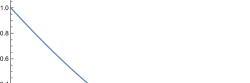
Figure 4. Graph of $f(x)$

It is curious to note that the sequence $\{a_{g,2},\,a_{g,5},\dots,a_{g,3j_{max}-1}\}$, where $j_{max}$ is the maximum integer satisfying $3j_{max}-1\leq\left[\frac{3g-1}{2}\right]$, is not monotonously increasing for $g\geq 17$. Let $x=\frac{j}{g}$. Our bounds on $j$ imply that $0<x<\frac{1}{2}$. For any fixed $g\gg 1$ define

$$f(x)=f\left(\frac{j}{g}\right)=\frac{(P_{1}(g,j)+P_{2}(g,j)+P_{3}(g,j))}{Q(g,j)}\,.$$

For large values of $g$ the graph of $f(x)$ has the form as in Figure 4, so up to some point the function $f$ remains positive and the sequence $a_{g,2},\,a_{g,5},\dots$ monotonously increases, but then it attains its maximum and very slowly monotonously decreases up to $a_{g,3j_{max}-1}$.

4.5. Asymptotic volume contribution of one-cylinder square-tiled surfaces.

In this section we compute the large genus asymptotics for the contributions of the stable graphs having a single edge to the Masur–Veech volume $\operatorname{Vol}\mathcal{Q}_{g}$ of the moduli space of holomorphic quadratic differentials on complex curves of genus $g$. In other words, we compute asymptotic contributions of one-cylinder square-tiled surfaces to the Masur–Veech volume of the principal stratum $\mathcal{Q}(1^{4g-4})$ of holomorphic quadratic differentials in large genus $g$. These contributions obviously provide lower bounds for $\operatorname{Vol}\mathcal{Q}_{g}$.

Denote by $\Gamma_{1}(g)$ the stable graph having a single vertex and having a single edge and such that the vertex is decorated with integer $g-1$ (see Figure 5). The single edges forms a loop, so this stable graphs represents a surface of genus $g$ with no marked points. This stable graph encodes the orbit of a simple closed nonseparating curve on a surface of genus $g$. This stable graph represents also the boundary divisor $\delta_{0,g}\subset\overline{\mathcal{M}}_{g}-\mathcal{M}_{g}$ for which the generic stable curve has single irreducible component of genus $g-1$ with single node.

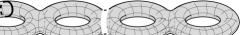
Figure 5. Graph $\Gamma_{1}(g)$ on the left represents non-separating simple closed curves on a surface of genus $g$ (as in the middle) and the boundary divisor $\delta_{0,g}$ of irreducible stable curves with single node as on the right.

Theorem 4.9.

The contribution of the graph $\Gamma_{1}(g)$ having single vertex decorated with label $g-1$ and single edge to the Masur–Veech volume $\operatorname{Vol}\mathcal{Q}_{g}$ of the moduli space $\mathcal{Q}_{g}$ of holomorphic quadratic differentials on complex curves of genus $g$ has the following asymptotics:

(4.30) $$\operatorname{Vol}\Gamma_{1}(g)=\sqrt{\frac{2}{3\pi g}}\cdot\left(\frac{8}{3}\right)^{4g-4}\cdot\left(1+O\left(\frac{1}{g}\right)\right)\quad\text{as }g\to+\infty\,.$$

Proof.

It would be slightly more convenient to prove formula (4.30) in genus $g+1$. Assign variable $b_{1}$ to the only edge of the graph. Formula (1.14) from Theorem 1.6 applied to the graph $\Gamma_{1}(g+1)$ gives

(4.31) $$\left(\frac{(4g)!}{(6g)!}\cdot 2^{6g}\cdot 12g\right)\cdot\frac{1}{2}\cdot 1\cdot b_{1}\cdot N_{g,2}(b_{1},b_{1})\xmapsto{\mathcal{Z}}\\ \xmapsto{\ \mathcal{Z}\ }\operatorname{Vol}\Gamma_{1}(g+1)=(4g)!\cdot 2^{g+2}\cdot\zeta(6g)\cdot\sum_{d_{1}+d_{2}=3g-1}\frac{\langle\psi_{1}^{d_{1}}\psi_{2}^{d_{2}}\rangle}{d_{1}!\cdot d_{2}!}=\\ =(4g)!\cdot 2^{g+2}\cdot\zeta(6g)\cdot\sum_{k=0}^{3g-1}\frac{\langle\tau_{k}\tau_{3g-1-k}\rangle_{g}}{k!\cdot(3g-1-k)!}\,.$$

Now pass to the normalization (4.2) of the correlators $\langle\tau_{k}\tau_{3g-1-k}\rangle_{g}$:

$$a_{g,k}=\frac{(2k+1)!!\cdot(6g-1-2k)!!}{(6g-1)!!}\cdot 24^{g}\cdot g!\cdot\langle\tau_{k}\tau_{3g-1-k}\rangle_{g}\,.$$

By Proposition 4.1, the $2$-correlators admit the following uniform bounds under such normalization:

$$1-\frac{2}{6g-1}\leq a_{g,k}\leq 1\,,\quad\text{for }k=0,1,\dots,3g-1\,.$$

Rewriting the expression (4.31) for $\operatorname{Vol}\Gamma_{1}(g+1)$ in terms of $a_{g,k}$ we get

(4.32) $$\operatorname{Vol}\Gamma_{1}(g+1)/\zeta(6g)=\\ =(4g)!\cdot 2^{g+2}\cdot\frac{(6g-1)!!}{24^{g}\cdot g!}\cdot\sum_{k=0}^{3g-1}\frac{a_{g,k}}{k!\cdot(2k+1)!!\cdot(3g-1-k)!\cdot(6g-1-2k)!!}\,.$$

Passing from double factorials to factorials,

$$(6g-1)!! =\frac{(6g)!}{(3g)!\cdot 2^{3g}}$$

$$(2k+1)!! =\frac{(2k+1)!}{k!\cdot 2^{k}}$$

$$(6g-1-2k)!! =\frac{(6g-1-2k)!}{(3g-1-k)!\cdot 2^{3g-k-1}}\,,$$

we rewrite and simplify expression (4.32) as follows:

(4.33) $$\operatorname{Vol}\Gamma_{1}(g+1)/\zeta(6g)=\\ =(4g)!\cdot 2^{g+2}\cdot\frac{1}{3^{g}\cdot 2^{3g}}\cdot\frac{1}{g!\cdot(3g)!}\cdot\frac{1}{2}\sum_{k=0}^{3g-1}\binom{6g}{2k+1}\cdot a_{g,k}=\\ =\frac{(4g)}{g!\cdot(3g)!}\cdot\frac{1}{3^{g}\cdot 2^{2g}}\cdot 2\sum_{k=0}^{3g-1}\binom{6g}{2k+1}\cdot a_{g,k}\,.$$

Combining the classical identity

$$\sum_{k=0}^{3g-1}\binom{6g}{2k+1}=2^{6g-1}$$

with bounds (4.4) we get the following bounds for $\operatorname{Vol}\Gamma_{1}(g+1)$:

(4.34) $$\binom{4g}{g}\cdot\left(\frac{2^{4}}{3}\right)^{g}\cdot\left(1-\frac{2}{6g-1}\right)\leq\operatorname{Vol}\Gamma_{1}(g+1)/\zeta(6g)\leq\binom{4g}{g}\cdot\left(\frac{2^{4}}{3}\right)^{g}\,.$$

Note that

$$\zeta(6g)\to 1\quad\text{as }g\to+\infty$$

and the convergence is exponentially fast.

Applying Stirling’s formula to factorials in the binomial coefficient $\binom{4g}{g}$ in the latter expression and simplifying we get

(4.35) $$\binom{4g}{g}=\sqrt{\frac{2}{3\pi g}}\cdot\left(\frac{2^{8}}{3^{3}}\right)^{g}\cdot\left(1+O\left(\frac{1}{g}\right)\right)\quad\text{as }g\to+\infty\,.$$

Combining the latter equality with bounds (4.34) we get the desired formula (4.30) in genus $g+1$:

$$\operatorname{Vol}\Gamma_{1}(g+1)=\sqrt{\frac{2}{3\pi g}}\cdot\left(\frac{8}{3}\right)^{4g}\cdot\left(1+O\left(\frac{1}{g}\right)\right)\quad\text{as }g\to+\infty\,.$$

∎

Remark 4.10.

Actually, we have very good control of asymptotic expansions of correlators $a_{g,k}$ in powers of $\frac{1}{g}$, see , so it would not be difficult to specify several terms of the asymptotic expansion of $O\left(\frac{1}{g}\right)$ in formula (4.30). We do not do it only because we do not currently see any specific need for a more precise expression.

Theorem 4.9 immediately implies Theorem 1.9.

We proceed with the remaining graph having single edge. This time it has two vertices joined by the edge as in Figure 6. The two vertices are decorated with strictly positive integers $g_{1},g_{2}\in{\mathbb{N}}$ such that $g_{1}+g_{2}=g$ (see Figure 5). Without loss of generality we may assume that $g_{1}\leq g_{2}$. This stable graph encodes the orbit of a simple closed curve separating the compact surface of genus $g$ without punctures into subsurfaces of genera $g_{1}$ and $g_{2}$. This stable graph represents also the boundary divisor $\delta_{g_{1},g}\subset\overline{\mathcal{M}}_{g}-\mathcal{M}_{g}$ for which a generic stable curve has two irreducible components of genera $g_{1}$ and $g_{2}$ respectively joined at a single node.

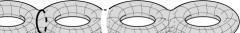
Figure 6. Graph $\Delta(g_{1},g_{2})$ represents simple closed curves on a surface of genus $g$ separating the surface into subsurfaces of genera $g_{1}$ and $g_{2}$, where $g_{1}+g_{2}=g$ (in the middle). The same graph represents the boundary divisor $\delta_{g_{1},g}\subset\overline{\mathcal{M}}_{g}-\mathcal{M}_{g}$ for which a generic stable curve has two irreducible components of genera $g_{1}$ and $g_{2}$ respectively joined at a single node (as on the right).

Proposition 4.11.

The contribution $\operatorname{Vol}(\Delta(g_{1},g-g_{1}))$ of the graph $\Delta(g_{1},g-g_{1})$ having a single edge joining two vertices decorated with labels $g_{1},g-g_{1}$ respectively, to the Masur–Veech volume $\operatorname{Vol}\mathcal{Q}_{g}$ of the moduli space $\mathcal{Q}_{g}$ of holomorphic quadratic differentials has the following value:

(4.36) $$\operatorname{Vol}(\Delta(g_{1},g-g_{1}))=\frac{4\cdot\zeta(6g-6)}{|\operatorname{Aut}(\Delta(g_{1},g-g_{1}))|}\cdot\binom{4g-4}{g}\cdot\frac{1}{12^{g}}\cdot\binom{g}{g_{1}}\cdot\binom{3g-4}{3g_{1}-2}\,.$$

Proof.

Let $g_{2}=g-g_{1}$. The contribution of the graph $\Delta(g_{1},g_{2})$ is given by formula (1.13) from Theorem 1.6:

(4.37) $$\operatorname{Vol}(\Delta(g_{1},g_{2}))=\frac{2^{6g-5}\cdot(4g-4)!}{(6g-7)!}\cdot\\ \frac{1}{2}\cdot\frac{1}{|\operatorname{Aut}(\Gamma(g_{1},g_{2}))|}\cdot\mathcal{Z}\big{(}b\cdot N_{g_{1},1}(b)\cdot N_{g_{2},1}(b)\big{)}\,,$$

where

(4.38) $$|\operatorname{Aut}(\Gamma(g_{1},g_{2}))|=\begin{cases}2,&\text{when }g_{1}=g_{2}\,,\\ 1,&\text{otherwise}\,.\end{cases}$$

By the result of E. Witten [Wi] one has the following closed expression for $1$-correlators:

$$\langle\psi_{1}^{3g-2}\rangle=\int_{\overline{\mathcal{M}}_{g,1}}\psi_{1}^{3g-2}=\frac{1}{24^{g}\cdot g!}\,.$$

Applying definitions (1.6) and (1.7) to $N_{g,1}(b)$ and using the above expression for $\langle\psi_{1}^{3g-2}\rangle$ we get the following close formula for the polynomial $N_{g,1}(b)$:

(4.39) $$N_{g,1}(b)=c_{3g-2}b^{2(3g-2)}=\frac{1}{2^{5g-6+2}\cdot(3g-2)!}\cdot\langle\psi_{1}^{3g-2}\rangle\cdot b^{6g-4}=\\ =\frac{1}{2^{8g-4}\cdot 3^{g}\cdot g!\cdot(3g-2)!}\cdot b^{6g-4}\,.$$

Using definition (1.11) of $\mathcal{Z}$ and the assumption $g_{1}+g_{2}=g$ we can now develop the rightmost factor in (1.11) as follows

$$\mathcal{Z}\big{(}b\cdot N_{g_{1},1}(b)\cdot N_{g_{2},1}(b)\big{)}=\\ =\mathcal{Z}\left(\frac{1}{2^{8g_{1}-4}\!\cdot\!2^{8g_{2}-4}}\!\cdot\!\frac{1}{3^{g_{1}}\!\cdot\!3^{g_{2}}}\!\cdot\!\frac{1}{g_{1}!\,g_{2}!}\!\cdot\!\frac{1}{(3g_{1}-2)!(3g_{2}-2)!}\!\cdot\!b\cdot b^{6g_{1}-4}\cdot b^{6g_{2}-4}\right)=\\ =\frac{1}{2^{8g-8}}\cdot\frac{1}{3^{g}}\cdot\frac{1}{g_{1}!\,(g-g_{1})!}\cdot\frac{1}{(3g_{1}-2)!(3g-3g_{1}-2)!}\cdot(6g-7)!\cdot\zeta(6g-6)\,.$$

Plugging this expression into (4.37); multiplying and dividing by $g!$ and by $(3g-4)!$ to pass to binomial coefficients and simplifying we get the desired formula (4.36). ∎

We complete this section with computation of cumulative contribution of the graphs $\Delta(g_{1},g-g_{1})$ to $\operatorname{Vol}\mathcal{Q}_{g}$ coming from all $g_{1}=1,\dots,\left[\frac{g}{2}\right]$.

Proposition 4.12.

The following asymptotic relation is valid

(4.40) $$\sum_{g_{1}=1}^{\left[\frac{g}{2}\right]}\operatorname{Vol}(\Delta(g_{1},g-g_{1}))\sim\frac{2}{3\pi g}\cdot\frac{1}{4^{g}}\cdot\left(\frac{8}{3}\right)^{4g-4}\,,$$

where the equivalence means that the ratio of the two expressions tends to $1$ as $g\to\infty$.

Proof.

Applying formula (4.37); making the summation index range from $1$ to $g-1$ (instead of up to $\left[\frac{g}{2}\right]$ and taking into consideration that when $g=2g_{1}$, the term $\operatorname{Vol}\Delta(g_{1},g_{1})$ has $|\operatorname{Aut}(\Delta(g_{1},g_{1}))|=2$ (see equation (4.38)) we get the following expression for the numerator of the latter expression:

$$\sum_{g_{1}=1}^{\left[\frac{g}{2}\right]}\operatorname{Vol}(\Delta(g_{1},g-g_{1}))=2\cdot\zeta(6g-6)\cdot\binom{4g-4}{g}\cdot\frac{1}{12^{g}}\cdot\sum_{g_{1}=1}^{g-1}\binom{g}{g_{1}}\cdot\binom{3g-4}{3g_{1}-2}\,.$$

The zeta value $\zeta(6g-6)$ tends to $1$ exponentially fast when $g\to+\infty$. Stirling Formula provides the follwing asymptotic value of the binomial coefficient

$$\binom{4g-4}{g}\sim\frac{1}{\sqrt{6\pi g}}\cdot 3^{g}\cdot\left(\frac{4}{3}\right)^{4g-4}\,.$$

Thus, to complete the proof of formula (1.40) and, thus, of Theorem 1.27, it remains to prove the Lemma below. ∎

Lemma 4.13.

The following asymptotic formula is valid:

(4.41) $$S(g)=\sum_{g_{1}=1}^{g-1}\binom{g}{g_{1}}\binom{3g-4}{3g_{1}-2}\sim\frac{1}{\sqrt{6\pi g}}\cdot 2^{4g-4}$$

as $g\to+\infty$.

Proof.

The probability density of the normal distribution $\mathcal{N}(\mu,\sigma^{2})$ is given by the function

$$f(x\,|\,\mu,\sigma^{2})=\frac{1}{\sqrt{2\pi\sigma^{2}}}\cdot e^{-\tfrac{(x-\mu)^{2}}{2\sigma^{2}}}\,.$$

Let $g$ be a large positive integer. After normalization by $2^{g}$ the distribution of binomial coefficients $\binom{g}{k}$, where $k=0,1,\dots,g$, tends to the normal distribution $\mathcal{N}\!\!\left(\tfrac{g}{2},\tfrac{g}{4}\right)$ as $g\to+\infty$.

Let $m$ be any positive integer which we use as a fixed parameter. The normalized distribution of binomial coefficients $\binom{m\cdot g}{k}$, where $k=0,1,\dots,m\cdot g$, tends to the normal distribution $\mathcal{N}\!\!\left(\tfrac{m\cdot g}{2},\tfrac{m\cdot g}{4}\right)$ as $g\to\infty$. Hence, the normalized distribution of binomial coefficients $\binom{m\cdot g}{m\cdot k}$, where $k=0,1,\dots,g$, tends to the normal distribution $\mathcal{N}\!\!\left(\tfrac{g}{2},\tfrac{g}{4m}\right)$ as $g\to+\infty$. In particular, letting $m=3$ we see that the normalized distribution of binomial coefficients $\binom{3g-4}{3k-2}$, where $k=1,\dots,g-1$, tends to the normal distribution $\mathcal{N}\!\!\left(\tfrac{g}{2},\tfrac{g}{12}-\tfrac{1}{9}\right)$.

The normalized distribution of the product of two normal distributions $\mathcal{N}(\mu,\sigma_{1}^{2})$ and $\mathcal{N}(\mu,\sigma_{1}^{2})$ sharing the same mean $\mu$ is the normal distribution $\mathcal{N}\!\!\left(\mu,\tfrac{\sigma_{1}^{2}\sigma_{2}^{2}}{\sigma_{1}^{2}+\sigma_{2}^{2}}\right)$. Hence, after normalization by $S(g)$, the product $\binom{g}{g_{1}}\binom{3g-4}{3g_{1}-2}$, of the two binomial distributions, where $g_{1}=1,\dots,g-1$, tends to the normal distribution $\mathcal{N}(g/2,\sigma^{2})$, where

$$\sigma^{2}=\frac{\tfrac{g}{4}\left(\tfrac{g}{12}-\tfrac{1}{9}\right)}{\tfrac{g}{4}+\left(\tfrac{g}{12}-\tfrac{1}{9}\right)}\sim\frac{g}{16}\,,\quad\text{as }g\to+\infty\,.$$

Thus, the asymptotic value of the sum $S(g)$ can be computed as the value of the product distribution $\binom{g}{g_{1}}\binom{3g-4}{3g_{1}-2}$ at $\mu=g/2$ multiplied by $\sqrt{2\pi\sigma^{2}}$, that is

(4.42) $$S(g)\sim\binom{g}{\left[\frac{g}{2}\right]}\cdot\binom{3g-4}{3\left[\frac{g}{2}\right]-2}\cdot\sqrt{2\pi\tfrac{g}{16}}\,.$$

From Stirling formula we get

$$\binom{2m}{m}\sim\frac{2^{2m}}{\sqrt{\pi m}}\quad\text{and}\quad\binom{2m+1}{m}\sim\frac{2^{2m+1}}{\sqrt{\pi m}}\,.$$

Applying these asymptotic formula to each of the binomial coefficients in (4.42) for even and odd values of $g$ respectively we get

$$S(g)\sim\frac{2^{g}}{\sqrt{\pi\tfrac{g}{2}}}\cdot\frac{2^{3g-4}}{\sqrt{\pi\tfrac{3g-4}{2}}}\cdot\frac{\sqrt{\pi g}}{\sqrt{8}}\sim\frac{1}{\sqrt{6\pi g}}\cdot 2^{4g-4}\,.$$

∎

Remark.

The hypergeometric sum $S(g)$ on the left hand side of (4.41) satisfies the following recursive relation obtained applying Zeilberger’s algorithm:

$$S(g+2)=2\cdot\frac{(324g^{4}+432g^{3}+123g^{2}-49g-8)}{(6g-1)(3g+4)(3g-1)(g+1)}\cdot S(g+1)+\\ +36\cdot\frac{(6g+5)(4g-1)(4g-3)}{(6g-1)(3g+4)(3g-1)}\cdot S(g)\,.$$

The asymptotic formula (4.41) from Lemma 4.13 admits the following immediate generalization.

Proposition 4.14.

Let $a_{i}\in{\mathbb{N}}$, $b_{i},c_{i}\in{\mathbb{Z}}$, where $i=1,\dots,p$; $r_{j}\in{\mathbb{N}}$, $s_{j},t_{j}\in{\mathbb{Z}}$, where $j=1,\dots,q$, be any collection of integer parameters satisfying the condition

$$(a_{1}+\dots+a_{p})-(r_{1}+\dots+r_{q})>0\,.$$

Let $n\in{\mathbb{N}}$. The following asymptotic formula is valid:

(4.43) $$\sum_{k=0}^{n}\frac{\begin{pmatrix}a_{1}n+b_{1}\\ a_{1}k+c_{1}\end{pmatrix}\cdots\begin{pmatrix}a_{p}n+b_{p}\\ a_{p}k+c_{p}\end{pmatrix}}{\begin{pmatrix}r_{1}n+s_{1}\\ r_{1}k+t_{1}\end{pmatrix}\cdots\begin{pmatrix}r_{q}n+s_{q}\\ r_{q}k+t_{q}\end{pmatrix}}\sim\\ \sim\rule{0.0pt}{20.0pt}\left(\frac{\pi n}{2}\right)^{\tfrac{q-p+1}{2}}\cdot 2^{(\sum_{i}a_{i}-\sum_{j}r_{j})n+(\sum_{i}b_{i}-\sum_{j}s_{j})}\cdot\left(\frac{\prod_{j}r_{j}}{\prod_{i}a_{i}}\right)^{\tfrac{1}{2}}\cdot\frac{1}{\left(\sum_{i}a_{i}-\sum_{j}r_{j}\right)^{\tfrac{1}{2}}}$$

as $n\to+\infty$.

By convention, the sum is evaluated only for those $k$ in the range $0,\dots,n$ for which all binomial coefficients in the numerator and in the numerator are well-defined, the sum $\sum_{j=1}^{q}r_{j}$ is equal to zero and the product $\prod_{j=1}^{q}r_{j}$ is equal to one when $q=0$.

4.6. Frequencies of simple closed geodesics

In this section we use the setting and the notations as in the Theorem 6.1 of M. Mirzakhani [Mi3] reproduced at the end of Section 1.2.

Recall that equivalence classes of smooth simple closed curves on an oriented surface of genus $g$ without boundary or punctures, where curves are considered up to a diffeomorphism are classified as follows. The curve can be separating or non-separating. All non-separating curves as in Figure 5 belong to the same class; we denote the corresponding frequency by $c(\gamma_{nonsep,g})$.

Separating simple closed curves are classified by the genera $g_{1},g_{2}$ of components in which the curve separates the surface; see Figure 6. Here $g_{1}+g_{2}=g$; $g_{1},g_{2}\geq 1$, and pairs $g_{1},g_{2}$ and $g_{2},g_{1}$ correspond to the same equivalence class. Denote a simple closed curve of this type by $\gamma_{g_{1},g_{2}}$.

Recall that reduced simple closed multicurves are in the natural bijective correspondence with stable graphs. The stable graph corresponding to $\gamma_{g_{1},g_{2}}$ is, clearly, $\Delta(g_{1},g_{2})$.

Recall that the volume contribution $\operatorname{Vol}(\Delta(g_{1},g_{2}))$ comes from all one-cylinder square-tiled surfaces of genus $g=g_{1}+g_{2}$ such that the waist curve of the single cylinder separates the surface into two surfaces of genera $g_{1}$ and $g_{2}$ respectively. This single horizontal cylinder can be composed of $a=1,2,\dots$ horizontal bands of squares. The contribution $\operatorname{Vol}(\Delta(g_{1},g_{2}))$ is the sum of contributions $\operatorname{Vol}(a\cdot\gamma_{g_{1},g_{2}})$ of square-tiled surfaces having fixed value $a\in{\mathbb{N}}$,

$$\operatorname{Vol}(\Delta(g_{1},g_{2}))=\sum_{a=1}^{+\infty}\operatorname{Vol}(a\cdot\gamma_{g_{1},g_{2}})\,.$$

Recall also, that

$$\operatorname{Vol}(a\cdot\gamma_{g_{1},g_{2}})=\frac{1}{a^{d}}\operatorname{Vol}(\gamma_{g_{1},g_{2}})\,,$$

where $d=6g-6=\dim\mathcal{Q}_{g}$, which implies that

$$\operatorname{Vol}(\Delta(g_{1},g_{2}))=\zeta(6g-6)\cdot\operatorname{Vol}(\gamma_{g_{1},g_{2}})\,.$$

Combining the latter relation with formula (1.30) from Theorem 1.20 we get

$$\frac{\operatorname{Vol}(\Delta(g_{1},g_{2}))}{\zeta(6g-6)}=\operatorname{Vol}(\gamma_{g_{1},g_{2}})=2\cdot(6g-6)\cdot(4g-4)!\cdot 2^{4g-3}\cdot c(\gamma_{g_{1},g_{2}})\,.$$

Applying expression (4.36) for $\operatorname{Vol}\Gamma(g_{1},g_{2})$ we get the following formula:

(4.44) $$c(\gamma_{g_{1},g-g_{1}})=\frac{1}{|\operatorname{Aut}\Delta(g_{1},g-g_{1})|}\cdot\\ \cdot\frac{1}{2^{3g-4}\cdot 24^{g}\cdot g_{1}!\cdot(g-g_{1})!\cdot(3g_{1}-2)!\cdot(3(g-g_{1})-2)!\cdot(6g-6)}\,.$$

In this way we reprove the formula for the frequency of simple closed separating geodesics first proved by M. Mirzakhani (see page 124 in [Mi3]).

Remark 4.15.

The formula on page 124 in [Mi3] contains two misprints: the power in the first factor in the denominator is indicated as $2^{3g-2}$ while it should be read as $2^{3g-4}$ and the fifth factor is indicated as $(3g-2)!$ while it should be read as $(3i-2)!$. Indeed, following Mirzakhani’s calculation we have to use formula (5.5) from [Mi3] for $c(\gamma)$. In notations of this formula applied to our particular $\gamma$ we have $n=0$, $k=1$, $a_{1}=1$, $s_{1}=3g-4$. Mirzakhani assumes for simplicity that $g>2i>2$, which implies that $M(\gamma)=0$ and $|\operatorname{Sym}(\gamma)|=1$ (and implies that $|\operatorname{Aut}\Delta(g_{1},g-g_{1})|=1$ in notations of Formula (4.44) above). Thus, applying formula (5.5) from [Mi3] she gets

$$c(\gamma)=b_{\Gamma}(2\cdot(3g-4))=(2\cdot(3g-4))_{\Gamma}\cdot\frac{(2\cdot(3g-4)+1)!}{(6g-6)!}\,.$$

To compute $(2\cdot(3g-4))_{\Gamma}$ we compute following Mirzakhani the product of the coefficients of the leading terms of the polynomials $V_{i,1}(x)$ and $V_{g-i,1}(x)$ (see the bottom of page 122 in [Mi3]). In this way we get

$$\frac{1}{(3i-2)!\cdot i!\cdot 24^{i}\cdot 2^{3i-2}}\cdot\frac{1}{(3(g-i)-2)!\cdot(g-i)!\cdot 2^{3(g-i)-2}}=\\ =\frac{1}{2^{3g-4}\cdot 24^{g}\cdot i!\cdot(g-i)!\cdot(3i-2)!\cdot(3(g-i)-2)!}\,.$$

(compare to (4.44) replacing $g_{1}$ with $i$). The remaining last factor $(6g-6)$ in the denominator of the formula of Mirzakhani comes from $\frac{(2\cdot(3g-4)+1)!}{(6g-6)!}=\frac{1}{6g-6}$.

Denote by $c(\gamma_{sep,g})$ the sum of the frequencies $c(\gamma_{g_{1},g_{2}})$ over all equivalence classes of separating curves, i.e. over all unordered pairs $(g_{1},g_{2})$ satisfying $g_{1}+g_{2}=g$; $g_{1},g_{2}\geq 1$. We are now ready to prove Theorem 1.27.

Proof of Theorem 1.27.

By Theorem 1.20 we have

$$\frac{c(\gamma_{sep,g})}{c(\gamma_{nonsep,g})}=\frac{\sum_{g_{1}=1}^{\left[\frac{g}{2}\right]}\operatorname{Vol}(\Delta(g_{1},g-g_{1}))}{\operatorname{Vol}\Gamma_{1}(g)}\,.$$

Plugging the asymptotic values (4.30) and (4.40) respectively in the denominator and numerator of the ratio on the right hand side we obtain the desired asymptotic value for the ratio on the left hand side. ∎

In the table below we present the exact (first line) and approximate (second line) values of the ratio $\tfrac{c(\gamma_{sep,g})}{c(\gamma_{nonsep,g})}$ of the two frequencies in small genera and the value given by the asymptotic formula (1.40) (third line).

$$\begin{array}[]{c|c|c|c|c||c}g&2&3&4&5&11\\ \hline\cr&&&&&\\[-6.0pt] \text{\small Exact}&\frac{1}{48}&\frac{5}{1776}&\frac{605}{790992}&\frac{4697}{27201408}&\frac{166833285883}{5360555755385245488}\\ &&&&&\\[-6.0pt] \hline\cr&&&&&\\[-6.0pt] \text{\small Approximate}&\scriptstyle 2.08\cdot 10^{-2}&\scriptstyle 2.82\cdot 10^{-3}&\scriptstyle 7.65\cdot 10^{-4}&\scriptstyle 1.73\cdot 10^{-4}&\scriptstyle 3.11\cdot 10^{-8}\\ &&&&&\\[-6.0pt] \hline\cr&&&&&\\[-6.0pt] \text{\small Asymp. formula}&\scriptstyle 2.03\cdot 10^{-2}&\scriptstyle 4.16\cdot 10^{-3}&\scriptstyle 9.00\cdot 10^{-4}&\scriptstyle 2.01\cdot 10^{-4}&\scriptstyle 3.31\cdot 10^{-8}\end{array}$$

Appendix A Stable graphs: formal definition

We now introduce the definition of a stable graph. Let $S$ be an hyperbolic surface of genus $g$ and $n$ (numbered) marked points. Let $\gamma$ be a multicurve on $S$ (that is a finite union of disjoint geodesics) the surface $S\setminus\gamma$ is a union of surfaces with boundaries (and marked points). The dual graph $\Gamma$ to this decomposition is constructed as follows:

• each subsurface gives rise to a vertex $v$ of $\Gamma$ carrying some genus $g_{v}$, some marked points (the legs) and a certain number of boundary components,

• each component $\gamma^{\prime}$ of $\gamma$ gives rise to an edge between the two components on the two sides of $\gamma^{\prime}$.

See the figures in the tables of Appendix B.1 for the correspondence between multicurves and stable graphs in genus 2.

We now introduce the more formal following definition.

Definition A.1.

A stable graph for $\mathcal{M}_{g,n}$ is a 6-tuple $\Gamma=(V,H,\alpha,\iota,\mathbf{g},L)$ where

• $V$ is a finite set of vertices

• $H$ is a finite set of half-edges

• $\iota:H\to H$ is an involution. The fixed points of $\iota$ are called the legs and the 2-cycles the edges of $\Gamma$.

• $\alpha:H\to V$ is a map that attaches an half-edge to a vertex. The number of half-edges at a given vertex $v$ is denoted by $n_{v}:=|\alpha^{-1}(v)|$.

• The graph is connected: for each pair of vertices $(u,v)$ there exists a sequence of half edges $(h_{1},h^{\prime}_{1},h_{2},h^{\prime}_{2},\ldots,h_{k},h^{\prime}_{k})$ so that $\iota(h_{i})=h^{\prime}_{i}$, $u=\alpha(h_{1})$, $v=\alpha(h^{\prime}_{k})$ and $\alpha(h^{\prime}_{i})=\alpha(h_{i+1})$..

• $\mathbf{g}=\{g_{v}\}_{v\in V}$ is a set of non-negative integers, one at each vertex, called the genus decoration.

• $L$ is a bijection from the set of legs to $\{1,\ldots,n\}$.

• The genus $g(\Gamma)$ of $\Gamma$ should be equal to $g$ where

  $$g(\Gamma)=h^{1}(\Gamma)+\sum_{v\in V}g_{v}$$

  where $h^{1}(\Gamma)$ is the first betti number of the graph.

• the following stability condition holds at each vertex $v$ of $\Gamma$

  $$2g_{v}-2+n_{v}>0.$$

Given a stable graph $\Gamma$, we associate an underlying graph whose vertex set is $V$ and each 2 cycle $(h,h^{\prime})$ of $\iota$ gives an edge attached to $\alpha(h)$ and $\alpha(h^{\prime})$. We denote $E=E(\Gamma)$ these edges. Such graph might have multiple edges and loops. The additional information of the stable graph is the genus decoration $\mathbf{g}$ and the $n$ legs.

Two stable graphs $\Gamma=(V,H,\mathbf{v},\iota,L,\mathbf{g})$ and $\Gamma^{\prime}=(V^{\prime},H^{\prime},\mathbf{v^{\prime}},\iota,L^{\prime},\mathbf{g^{\prime}})$ are isomorphic if there exists two bijections $\phi:V\to V^{\prime}$ and $\psi:H\to H^{\prime}$ that preserve edges, legs and markings that is

$$\iota\circ\psi=\iota^{\prime}\circ\psi\quad L^{\prime}(\psi(h))=L(h)\quad g^{\prime}_{\phi(v)}=g_{v}.$$

The definition of stable graphs and automorphisms mean that neither vertices nor edges of the decorated graph $\Gamma$ are labeled, but each leg is numbered by $L$.

We denote by $\mathcal{G}_{g,n}$ the set of isomorphism classes of stable graphs with given genus $g$ and number of legs $n$.

As we already mentioned, each stable graph in $\mathcal{G}_{g,n}$ corresponds to a bounary cycle of the Deligne-Mumford compactification $\overline{\mathcal{M}_{g,n}}$. More precisely, each vertex $v$ of the graph corresponds to the component of a nodal curve (of genus $g_{v}$ and contain the marked points corresponding to the legs attached at this vertex) and each edge of $E(\Gamma)$ represents a node together with its number in $\{1,2,\ldots,n\}$. (See survey [Va] for excellent introduction in this subject and for beautiful illustrations.) Hence, the unique stable graph with no edge and $n$ legs in $\mathcal{G}_{g,n}$ corresponds to the component $\mathcal{M}_{g,n}$ (the smooth curves).

Appendix B Examples of explicit calculations

B.1. Holomorphic quadratic differentials in genus two.

We start by evaluation of the Siegel–Veech constant $c_{\mathit{area}}(Q_{2})$. Note that certain graphs do not contribute at all to $c_{\mathit{area}}$.

$$\hskip 20.0pt\begin{array}[]{ll|l}\ltx@special@graphics[voffset={-10},hoffset={-15},hscale={20},vscale={20},angle={0}]{genus_two_21.eps}\begin{picture}(0.0,0.0)(0.0,0.0)\put(-24.0,0.0){$b_{1}$} \put(66.0,0.0){$b_{2}$} \end{picture}\par&\frac{128}{5}\cdot 1\cdot\frac{1}{8}\cdot b_{1}b_{2}\cdot N_{0,4}(b_{1},b_{1},b_{2},b_{2})=\par&(1+1)\cdot\par\\ \ltx@special@graphics[voffset={-15},hoffset={0},hscale={25},vscale={25},angle={0}]{genus_two_graph_21.eps}\begin{picture}(0.0,0.0)(0.0,-10.0)\put(-9.0,-19.0){$b_{1}$} \put(52.0,-19.0){$b_{2}$} \put(23.0,-30.0){$0$} \end{picture}\par&\rule{0.0pt}{12.0pt}=\frac{16}{5}\cdot b_{1}b_{2}\cdot\left(\frac{1}{4}(2b_{1}^{2}+2b_{2}^{2})\right)\par&\cdot\!\frac{8}{5}\!\cdot\!3!\zeta(4)\!\cdot\!1!\zeta(2)\par\par\\ &\hskip 45.0pt\xmapsto{\partial_{\Gamma}}\frac{8}{5}(1\cdot b_{1}b_{2}^{3}+1\cdot b_{1}^{3}b_{2})\xmapsto{\mathcal{Z}}\par&=1\cdot\frac{8}{225}\cdot\pi^{6}\par\\ \vspace*{-18pt}\\ &&\\ \hline\cr&&\\ \ltx@special@graphics[voffset={-10},hoffset={-15},hscale={20},vscale={20},angle={0}]{genus_two_22.eps}\begin{picture}(0.0,0.0)(0.0,0.0)\put(-24.0,0.0){$b_{1}$} \put(23.0,-14.0){$b_{2}$} \end{picture}\rule{0.0pt}{12.0pt}\par\par&\frac{128}{5}\!\cdot\!\frac{1}{2}\!\cdot\!\frac{1}{2}\!\cdot\!b_{1}b_{2}\!\cdot\!N_{0,3}(b_{1},b_{1},b_{2})\!\cdot\!N_{1,1}(b_{2})\par&1\!\cdot\!\frac{2}{15}\!\cdot\!1!\zeta(2)\!\cdot\!3!\zeta(4)\par\\ \ltx@special@graphics[voffset={-15},hoffset={-10},hscale={25},vscale={25},angle={0}]{genus_two_graph_22.eps}\begin{picture}(0.0,0.0)(0.0,0.0)\put(-19.0,-10.0){$b_{1}$} \put(23.0,-16.0){$b_{2}$} \put(6.0,-10.0){$0$} \put(41.0,-10.0){$1$} \end{picture}\par&\rule{0.0pt}{15.0pt}=\frac{32}{5}\!\cdot\!b_{1}b_{2}\!\cdot\!1\!\cdot\!\left(\frac{1}{48}b_{2}^{2}\right)\xmapsto{\partial_{\Gamma}}\!\frac{2}{15}\!\cdot\!1\!\cdot\!b_{1}b_{2}^{3}\xmapsto{\mathcal{Z}}&=1\cdot\frac{1}{675}\cdot\pi^{6}\par\\ &&\\ \vspace*{-18pt}\\ &&\\ \hline\cr&&\\ \ltx@special@graphics[voffset={-10},hoffset={-15},hscale={20},vscale={20},angle={0}]{genus_two_31.eps}\begin{picture}(0.0,0.0)(0.0,0.0)\put(-24.0,0.0){$b_{1}$} \put(23.0,-14.0){$b_{2}$} \put(66.0,0.0){$b_{3}$} \end{picture}\par&\frac{128}{5}\!\cdot\!\frac{1}{2}\!\cdot\!\frac{1}{8}\!\cdot\!b_{1}b_{2}b_{3}\!\cdot\!N_{0,3}(b_{1},b_{1},b_{2})\cdot\par&(1+\frac{1}{2}+1)\cdot\par\\ \ltx@special@graphics[voffset={-20},hoffset={-10},hscale={25},vscale={25},angle={0}]{genus_two_graph_31.eps}\begin{picture}(0.0,0.0)(0.0,5.0)\put(-18.0,-10.0){$b_{1}$} \put(23.0,-16.0){$b_{2}$} \put(63.0,-10.0){$b_{3}$} \put(5.5,-10.0){$0$} \put(42.0,-10.0){$0$} \end{picture}\par\rule{0.0pt}{12.0pt}\par&\cdot N_{0,3}(b_{2},b_{3},b_{3})=\frac{8}{5}\!\cdot\!{b_{1}}{b_{2}}{b_{3}}\!\cdot\!(1)\!\cdot\!(1)\par\par&\cdot\frac{8}{5}\cdot\left(1!\,\zeta(2)\right)^{3}\\ &\rule{0.0pt}{15.0pt}\xmapsto{\partial_{\Gamma}}\!\frac{8}{5}\!\left(1\!\cdot\!b_{1}b_{2}b_{3}\!+\!\frac{1}{2}b_{1}b_{2}b_{3}\!+\!1\!\cdot\!b_{1}b_{2}b_{3}\right)\!\!\xmapsto{\mathcal{Z}}\!&=\frac{5}{2}\cdot\frac{1}{135}\cdot\pi^{6}\par\\ \vspace*{-18pt}\\ &&\\ \hline\cr&&\\ \ltx@special@graphics[voffset={-10},hoffset={-15},hscale={20},vscale={20},angle={0}]{genus_two_32.eps}\begin{picture}(0.0,0.0)(0.0,0.0)\put(-24.0,0.0){$b_{1}$} \put(20.0,12.0){$b_{2}$} \put(66.0,0.0){$b_{3}$} \end{picture}\par&\frac{128}{5}\!\cdot\!\frac{1}{2}\!\cdot\!\frac{1}{12}\!\cdot\!b_{1}b_{2}b_{3}\!\cdot\!N_{0,3}(b_{1},b_{1},b_{2})\cdot\par&(1+1+1)\cdot\par\\ \ltx@special@graphics[voffset={-32},hoffset={42},hscale={25},vscale={25},angle={90}]{genus_two_graph_32.eps}\begin{picture}(0.0,0.0)(0.0,0.0)\put(4.0,-16.0){$b_{1}$} \put(27.5,-16.0){$b_{2}$} \put(43.0,-16.0){$b_{3}$} \put(31.0,2.0){$0$} \put(31.0,-35.0){$0$} \end{picture}\par&\rule{0.0pt}{15.0pt}\par\cdot N_{0,3}(b_{2},b_{3},b_{3})=\frac{16}{15}\!\cdot\!{b_{1}b_{2}b_{3}}\!\cdot\!(1)\!\cdot\!(1)\par\par&\frac{16}{15}\!\cdot\!\left(1!\,\zeta(2)\right)^{3}\\ &\rule{0.0pt}{15.0pt}\par\xmapsto{\partial_{\Gamma}}\!\frac{8}{5}\!\left(1\!\cdot\!b_{1}b_{2}b_{3}\!+\!\frac{1}{2}b_{1}b_{2}b_{3}\!+\!1\!\cdot\!b_{1}b_{2}b_{3}\right)\!\!\xmapsto{\mathcal{Z}}\!&=3\cdot\frac{2}{405}\cdot\pi^{6}\end{array}$$

Taking the sum of the four contributions we obtain:

$$\left(\left(1\cdot\frac{8}{225}+1\cdot\frac{1}{675}\right)+\left(\frac{5}{2}\cdot\frac{1}{135}+3\cdot\frac{2}{405}\right)\right)\cdot\pi^{6}=\left(\frac{1}{27}+\frac{1}{30}\right)\cdot\pi^{6}=\frac{19}{270}\cdot\pi^{6}\,.$$

Dividing by $\operatorname{Vol}\mathcal{Q}(1^{4})=\cfrac{1}{15}\cdot\pi^{6}$ we get the answer which matches the value found in [G1]: $\cfrac{\pi^{2}}{3}\cdot c_{area}(\mathcal{Q}(1^{4}))=\left(\cfrac{19}{270}\pi^{6}\right):\left(\cfrac{1}{15}\pi^{6}\right)=\cfrac{19}{18}\,.$

The computation of the Masur–Veech volume $\operatorname{Vol}\mathcal{Q}_{2}$ was presented in Table 1 in Section 1.4. The first two graphs in Table 1 represent the contribution to the volume $\operatorname{Vol}\mathcal{Q}(1^{4})$ of square-tiled surfaces having single maximal cylinder. The resulting contribution $\frac{7}{405}\pi^{6}=\frac{49}{3}\zeta(6)$ was found in Appendix C in [DGZZ1] by completely different technique.

The third and the fourth graph together represent the contribution $\frac{1}{27}\pi^{6}$ of square-tiled surfaces having two maximal cylinders. The last two graphs — the contribution $\frac{1}{81}\pi^{6}$ of square-tiled surfaces having three maximal cylinders.

Normalizing the contribution of $1,2,3$-cylinder square-tiled surfaces by the entire volume $\operatorname{Vol}\mathcal{Q}(1^{4})$ of the stratum we get the quantity $p_{k}(\mathcal{Q}(1^{4}))$ which can be interpreted as the “probability” for a “random” square-tiled surface in the stratum $\mathcal{Q}(1^{4})$ to have exactly $k$ horizontal cylinders. These same quantities $p_{k}$ provide “probabilities” of getting a $k$-band generalized interval exchange transformation (linear involution) taking a “random” generalized interval exchange transformation in the Rauzy class representing the stratum $\mathcal{Q}(1^{4})$ (see section 3.2 in [DGZZ1] for details). The latter quantities are particularly simple to evaluate in numerical experiments. The resulting proportions

$$\big{(}p_{1}(\mathcal{Q}(1^{4})),p_{2}(\mathcal{Q}(1^{4})),p_{3}(\mathcal{Q}(1^{4}))\big{)}=\left(\frac{7}{405},\frac{1}{27},\frac{1}{81}\right):\frac{1}{15}=\left(\frac{7}{27},\frac{15}{27},\frac{5}{27}\right)$$

match the numerical experiments obtained earlier in Appendix C of [DGZZ1].

B.2. Holomorphic quadratic differentials in genus three.

In genus three there are already $41$ different decorated ribbon graphs. We do not provide the graph-by-graph calculation as we did in genus two but only the contributions of $k$-cylinder square-tiled surfaces for all possible values $k=1,\dots,6$ of cylinders.

$$\begin{array}[]{|c|c|c|c|}\hline\cr&&&\\[-6.0pt] \text{Number of}&\text{Number of}&\text{Contribution}&\text{Relative}\\ \text{cylinders }k&\text{graphs }\Gamma&\text{to the volume}&\text{contribution }p_{k}\\ &&&\\[-6.0pt] \hline\cr&&&\\[-6.0pt] 1&2&\frac{94667}{126299250}\cdot\pi^{12}&\frac{757336}{3493125}\\ &&&\\[-6.0pt] \hline\cr&&&\\[-6.0pt] 2&5&\frac{150749}{108256500}\cdot\pi^{12}&\frac{4220972}{10479375}\\ &&&\\[-6.0pt] \hline\cr&&&\\[-6.0pt] 3&9&\frac{84481}{86605200}\cdot\pi^{12}&\frac{591367}{2095875}\\ &&&\\[-6.0pt] \hline\cr&&&\\[-6.0pt] 4&12&\frac{5989}{21651300}\cdot\pi^{12}&\frac{167692}{2095875}\\ &&&\\[-6.0pt] \hline\cr&&&\\[-6.0pt] 5&8&\frac{1}{17820}\cdot\pi^{12}&\frac{28}{1725}\\ &&&\\[-6.0pt] \hline\cr&&&\\[-6.0pt] 6&5&\frac{1}{144342}\cdot\pi^{12}&\frac{56}{27945}\\ &&&\\ \hline\cr\end{array}$$

The resulting contribution of $1$-cylinder surfaces was confirmed by the alternative combinatorial study of the Rauzy class of the stratum $\mathcal{Q}(1^{8})$ (see section 3.2 in [DGZZ1]. The approximate values $p_{k}(\mathcal{Q}(1^{8}))$ were confirmed by numerical experiments with statistics of $k$-band generalized interval exchange transformations.

Taking the sum of all contributions we get the volume of the moduli space $\mathcal{Q}_{3}$ of holomorphic quadratic differentials in genus $3$: $\operatorname{Vol}\mathcal{Q}_{3}=\cfrac{115}{33264}\cdot\pi^{12}\,.$

B.3. Meromorphic quadratic differentials in genus one.

In this section we apply formula (1.13) to compute the Masur–Veech volume $\operatorname{Vol}\mathcal{Q}(1^{2},-1^{2})$ of the moduli space $\mathcal{Q}_{1,2}$ of meromorphic quadratic differentials in genus $g=1$ with two simple poles $p=2$.

We use the same convention on the order of numerical factors in every first line of the middle column as in section B.1. Namely, for $(g,p)=(1,2)$ we have $\ell!\cdot 2d\cdot\frac{2^{d}}{d!}=\frac{32}{5}\,,$ which is the first factor. The second factor is $1/2^{|V(\Gamma)|-1}$.

The third factor is $|\operatorname{Aut}(\Gamma)|^{-1}$. We remind that the vertices and edges of $\Gamma$ are not labeled while the two legs are labeled. An automorphism of $\Gamma$ preserves the decoration of vertices and the labeling of the legs. For example, the graph $\Gamma$ in the second line does not have any nontrivial automorphisms.

$$\hskip 20.0pt\begin{array}[]{llr}\ltx@special@graphics[voffset={-10},hoffset={0},hscale={20},vscale={20},angle={0}]{genus_one_11.eps}\begin{picture}(0.0,0.0)(0.0,0.0)\put(-9.0,0.0){$b_{1}$} \end{picture}\par\vspace*{10pt}&\frac{32}{3}\cdot 1\cdot\frac{1}{2}\cdot b_{1}\cdot N_{0,4}(b_{1},b_{1},0,0)=\par&\\ \ltx@special@graphics[voffset={-4},hoffset={ 21},hscale={20},vscale={20},angle={0}]{genus_one_graph_11.eps}\begin{picture}(0.0,0.0)(0.0,0.0)\put(12.0,0.0){$b_{1}$} \put(40.0,-9.0){$0$} \end{picture}\par\vspace*{10pt}&\hskip 17.0pt=\frac{16}{3}\cdot b_{1}\cdot\left(\frac{1}{4}(2b_{1}^{2})\right)\hskip 5.0pt=\hskip 5.0pt\frac{8}{3}\cdot b_{1}^{3}\ \hskip 1.0pt\xmapsto{\ \mathcal{Z}\ }\par&\frac{8}{3}\cdot 3!\cdot\zeta(4)=\frac{8}{45}\pi^{4}\par\\ \hline\cr&&\\ \ltx@special@graphics[voffset={-10},hoffset={0},hscale={20},vscale={20},angle={0}]{genus_one_12.eps}\begin{picture}(0.0,0.0)(0.0,0.0)\put(38.0,12.0){$b_{1}$} \end{picture}\par\vspace*{10pt}&\frac{32}{3}\cdot\frac{1}{2}\cdot 1\cdot b_{1}\cdot N_{1,1}(b_{1})\cdot N_{0,3}(0,0,b_{1})=\par&\\ \ltx@special@graphics[voffset={-2.5},hoffset={21},hscale={20},vscale={20},angle={0}]{genus_one_graph_12.eps}\begin{picture}(0.0,0.0)(0.0,0.0)\put(29.0,5.0){$b_{1}$} \put(22.0,-9.0){$1$} \put(39.5,-9.0){$0$} \end{picture}\par\vspace*{10pt}&\hskip 17.0pt=\frac{16}{3}\cdot b_{1}\cdot\left(\frac{1}{48}b_{1}^{2}\right)\cdot(1)=\frac{1}{9}\cdot b_{1}^{3}\ \xmapsto{\ \mathcal{Z}\ }\par&\frac{1}{9}\cdot 3!\cdot\zeta(4)=\frac{1}{135}\cdot\pi^{4}\par\\ \hline\cr&&\\ \ltx@special@graphics[voffset={-10},hoffset={0},hscale={20},vscale={20},angle={0}]{genus_one_21.eps}\begin{picture}(0.0,0.0)(0.0,0.0)\put(-9.0,0.0){$b_{1}$} \put(38.0,12.0){$b_{2}$} \end{picture}\par\vspace*{10pt}&\frac{32}{3}\cdot\frac{1}{2}\cdot\frac{1}{2}\cdot b_{1}b_{2}\cdot N_{0,3}(b_{1},b_{1},b_{2})\cdot N_{0,3}(b_{1},0,0)\par&\\ \ltx@special@graphics[voffset={-4},hoffset={4},hscale={20},vscale={20},angle={0}]{genus_one_graph_21.eps}\begin{picture}(0.0,0.0)(0.0,0.0)\put(-5.0,0.0){$b_{1}$} \put(29.0,5.0){$b_{2}$} \put(22.0,-9.0){$0$} \put(39.5,-9.0){$0$} \end{picture}\par\vspace*{10pt}&\hskip 17.0pt=\frac{8}{3}\cdot b_{1}b_{2}\cdot(1)\cdot(1)=\frac{8}{3}\cdot b_{1}b_{2}\ \hskip 1.0pt\xmapsto{\ \mathcal{Z}\ }\par&\frac{8}{3}\cdot\big{(}\zeta(2)\big{)}^{2}=\frac{2}{27}\pi^{4}\par\\ \hline\cr&&\\ \ltx@special@graphics[voffset={-10},hoffset={0},hscale={20},vscale={20},angle={0}]{genus_one_22.eps}\begin{picture}(0.0,0.0)(0.0,0.0)\put(-9.0,0.0){$b_{1}$} \put(38.0,12.0){$b_{2}$} \end{picture}\par\vspace*{15pt}&\frac{32}{3}\cdot\frac{1}{2}\cdot\frac{1}{2}\cdot b_{1}b_{2}\cdot N_{0,3}(0,b_{1},b_{2})\cdot N_{0,3}(b_{1},b_{2},0)\par&\\ \ltx@special@graphics[voffset={-14},hoffset={25},hscale={20},vscale={20},angle={0}]{genus_one_graph_22.eps}\begin{picture}(0.0,0.0)(0.0,0.0)\put(15.0,0.0){$b_{1}$} \put(41.0,0.0){$b_{2}$} \put(29.5,1.5){$0$} \put(29.5,-20.0){$0$} \end{picture}\par\vspace*{20pt}&\hskip 17.0pt=\frac{8}{3}\cdot b_{1}b_{2}\cdot(1)\cdot(1)=\frac{8}{3}\cdot b_{1}b_{2}\par\ \hskip 1.0pt\xmapsto{\ \mathcal{Z}\ }\par&\frac{8}{3}\cdot\big{(}\zeta(2)\big{)}^{2}=\frac{2}{27}\pi^{4}\end{array}$$

Table 2. Computation of $\operatorname{Vol}\mathcal{Q}_{1,2}$. Left column represents stable graphs $\Gamma\in\mathcal{G}_{1,2}$ and associated multicurves; middle column gives associated polynomials $P_{\Gamma}$; right column provides $\operatorname{Vol}(\Gamma)$.

The resulting value

$$\operatorname{Vol}\mathcal{Q}_{1,2}=\left(\left(\frac{8}{45}+\frac{1}{135}\right)+\left(\frac{2}{27}+\frac{2}{27}\right)\right)\cdot\pi^{4}=\left(\frac{5}{27}+\frac{4}{27}\right)\cdot\pi^{4}=\cfrac{\pi^{4}}{3}$$

matches the one found in [G2]. The contribution of $1$-cylinder square-tiled surfaces and the proportion $5:4$ between $1$-cylinder and $2$-cylinder contributions match the corresponding quantities found in Appendix C in [DGZZ1].

Now we evaluate the Siegel–Veech constant $c_{\mathit{area}}(Q(1^{4}))$.

$$\hskip 5.0pt\begin{array}[]{llr}\ltx@special@graphics[voffset={-10},hoffset={0},hscale={20},vscale={20},angle={0}]{genus_one_21.eps}\begin{picture}(0.0,0.0)(0.0,0.0)\put(-9.0,0.0){$b_{1}$} \put(38.0,12.0){$b_{2}$} \end{picture}\vspace*{10pt}&\frac{32}{3}\cdot\frac{1}{2}\cdot\frac{1}{2}\cdot b_{1}b_{2}\cdot N_{0,3}(b_{1},b_{1},b_{2})\cdot N_{0,3}(b_{1},0,0)\par&\\ \ltx@special@graphics[voffset={-4},hoffset={4},hscale={20},vscale={20},angle={0}]{genus_one_graph_21.eps}\begin{picture}(0.0,0.0)(0.0,0.0)\put(-5.0,0.0){$b_{1}$} \put(29.0,5.0){$b_{2}$} \put(22.0,-9.0){$0$} \put(39.5,-9.0){$0$} \end{picture}\par\vspace*{10pt}&=\frac{8}{3}\cdot b_{1}b_{2}\cdot 1\cdot 1=\frac{8}{3}\cdot b_{1}b_{2}\ \xmapsto{\mathcal{Z}\circ\partial_{\Gamma}}\par&\left(1+\frac{1}{2}\right)\cdot\frac{8}{3}\cdot\big{(}\zeta(2)\big{)}^{2}=\frac{3}{2}\cdot\frac{2}{27}\pi^{4}\par\\ \hline\cr&&\\ \ltx@special@graphics[voffset={-10},hoffset={0},hscale={20},vscale={20},angle={0}]{genus_one_22.eps}\begin{picture}(0.0,0.0)(0.0,0.0)\put(-9.0,0.0){$b_{1}$} \put(38.0,12.0){$b_{2}$} \end{picture}\par\vspace*{15pt}&\frac{32}{3}\cdot\frac{1}{2}\cdot\frac{1}{2}\cdot b_{1}b_{2}\cdot N_{0,3}(0,b_{1},b_{2})\cdot N_{0,3}(b_{1},b_{2},0)\par&\\ \ltx@special@graphics[voffset={-14},hoffset={25},hscale={20},vscale={20},angle={0}]{genus_one_graph_22.eps}\begin{picture}(0.0,0.0)(0.0,0.0)\put(15.0,0.0){$b_{1}$} \put(41.0,0.0){$b_{2}$} \put(29.5,1.5){$0$} \put(29.5,-20.0){$0$} \end{picture}\par\vspace*{20pt}&=\frac{8}{3}\cdot b_{1}b_{2}\cdot 1\cdot 1=\frac{8}{3}\cdot b_{1}b_{2}\par\ \hskip 1.0pt\xmapsto{\mathcal{Z}\circ\partial_{\Gamma}}\par&(1+1)\cdot\frac{8}{3}\cdot\big{(}\zeta(2)\big{)}^{2}=2\cdot\frac{2}{27}\pi^{4}\end{array}$$

Taking the sum of the two contributions we obtain the answer:

$$\left(\frac{3}{2}\cdot\frac{2}{27}+2\cdot\frac{2}{27}\right)\cdot\pi^{4}=\frac{7}{27}\cdot\pi^{4}\,.$$

Dividing by $\operatorname{Vol}\mathcal{Q}(1^{2},-1^{2})=\frac{\pi^{4}}{3}$ we get the answer which matches the value found in [G1].

$$\frac{\pi^{2}}{3}\cdot c_{area}(\mathcal{Q}(1^{2},-1^{2}))=\left(\frac{7}{27}\cdot\pi^{4}\right):\left(\frac{1}{3}\cdot\pi^{4}\right)=\frac{7}{9}\,.$$

Appendix C Tables of volumes and of Siegel–Veech constants

In this appendix we present numerical data for $\mathcal{Q}_{g,n}$ corresponding to small values of $g$ and $n$. We apply formulae (1.13) and (1.25) respectively to express in Tables 3 and 4 the Masur–Veech volumes $\operatorname{Vol}(\mathcal{Q}_{g,n})$ and the Siegel–Veech constants $c_{\mathit{area}}(\mathcal{Q}_{g,n})$ as polynomials in the intersection numbers.

Recall that applying formula (1.26), one can express the Siegel–Veech constant $c_{\mathit{area}}$ in terms of the volumes of the principal boundary strata. Table 4 provides the corresponding explicit expressions for low-dimensional strata.

Finally, Table 5 gathers the numerical values of the volumes, of the Siegel–Veech constants and of the sums of the Lyapunov exponents of the low-dimensional strata $\mathcal{Q}(1^{\ell},-1^{p})$. (Recall that the stratum $\mathcal{Q}(1^{\ell},-1^{p})$ is open and dense in $\mathcal{Q}_{g,n}$, where $p=n$ and $l=4g-4+n$.) By formula 2.3 in [EKoZo], these quantities are related as follows:

$$\Lambda^{+}=\frac{1}{24}\left(\frac{5}{3}\ell-3p\right)+\frac{\pi^{2}}{3}c_{\mathit{area}}(\mathcal{Q}(1^{\ell},-1^{p}))\,.$$

The sum $\Lambda^{+}=\lambda_{1}^{+}+\dots+\lambda_{g}^{+}$ of the top $g$ Lyapunov exponents of the stratum $\mathcal{Q}(1^{\ell},-1^{p})$ admits experimental evaluation. The values of $\Lambda^{+}$ based on the values of $c_{\mathit{area}}(\mathcal{Q}(1^{\ell},-1^{p}))$ computed in this paper match the approximate values obtained in these numerical experiments.

One has $\Lambda^{+}=0$ in genus zero, so in genus zero the Siegel–Veech constant admits a simple closed formula. By formula 1.1 in [AEZ2] one has

$$\operatorname{Vol}\mathcal{Q}(1^{p-4},-1^{p})=2\pi^{2}\left(\frac{\pi^{2}}{2}\right)^{p-4}\,.$$

We get the same expressions in the entries of Table 5 corresponding to genus $0$ computed by formulae (1.13) and (1.25) of the current paper.

$\begin{array}[]{|c|c|c|}\hline\cr g&p&\operatorname{Vol}\mathcal{Q}(1^{4g-4+p},-1^{p})\\ \hline\cr 0&4&12\zeta(2)\langle\tau_{0}^{3}\rangle^{2}\\ \cline{3-3}\cr&&2\pi^{2}\langle\tau_{0}^{3}\rangle^{2}\\ \hline\cr 0&5&40\zeta(4)\langle\tau_{0}^{3}\tau_{1}\rangle\langle\tau_{0}^{3}\rangle+20\zeta(2)^{2}\langle\tau_{0}^{3}\rangle^{3}\\ \cline{3-3}\cr&&\frac{\pi^{4}}{9}(4\langle\tau_{0}^{3}\tau_{1}\rangle\langle\tau_{0}^{3}\rangle+5\langle\tau_{0}^{3}\rangle^{3})\\ \hline\cr 0&6&20\zeta(6)(4\langle\tau_{0}^{3}\tau_{1}\rangle^{2}+3\langle\tau_{0}^{4}\tau_{2}\rangle\langle\tau_{0}^{3}\rangle)+120\zeta(4)\zeta(2)\langle\tau_{0}^{3}\tau_{1}\rangle\langle\tau_{0}^{3}\rangle^{2}+28\zeta(2)^{3}\langle\tau_{0}^{3}\rangle^{4}\\ \cline{3-3}\cr&&\pi^{6}(\frac{16}{189}\langle\tau_{0}^{3}\tau_{1}\rangle^{2}+\frac{4}{63}\langle\tau_{0}^{4}\tau_{2}\rangle\langle\tau_{0}^{3}\rangle+\frac{2}{9}\langle\tau_{0}^{3}\tau_{1}\rangle\langle\tau_{0}^{3}\rangle^{2}+\frac{7}{54}\langle\tau_{0}^{3}\rangle^{4})\\ \hline\cr 1&2&16\zeta(4)(\langle\tau_{1}\rangle\langle\tau_{0}^{3}\rangle+\langle\tau_{0}^{3}\tau_{1}\rangle)+\frac{16}{3}\zeta(2)^{2}\langle\tau_{0}^{3}\rangle^{2}\\ \cline{3-3}\cr&&\frac{4\pi^{4}}{135}\big{(}6(\langle\tau_{1}\rangle\langle\tau_{0}^{3}\rangle+\langle\tau_{0}^{3}\tau_{1}\rangle)+5\langle\tau_{0}^{3}\rangle^{2}\big{)}\\ \hline\cr 1&3&24\zeta(6)(\langle\tau_{0}^{4}\tau_{2}\rangle+\langle\tau_{0}^{3}\tau_{1}^{2}\rangle+2\langle\tau_{1}\rangle\langle\tau_{0}^{3}\tau_{1}\rangle+3\langle\tau_{0}\tau_{2}\rangle\langle\tau_{0}^{3}\rangle)\\ &&+\frac{24}{5}\zeta(2)\zeta(4)(8\langle\tau_{0}^{3}\tau_{1}\rangle\langle\tau_{0}^{3}\rangle+3\langle\tau_{1}\rangle\langle\tau_{0}^{3}\rangle^{2})+\frac{32}{5}\zeta(2)^{3}\langle\tau_{0}^{3}\rangle^{3}\\ \cline{3-3}\cr&&\frac{\pi^{6}}{45}\big{(}\frac{8}{7}(\langle\tau_{0}^{4}\tau_{2}\rangle+\langle\tau_{0}^{3}\tau_{1}^{2}\rangle+2\langle\tau_{1}\rangle\langle\tau_{0}^{3}\tau_{1}\rangle+3\langle\tau_{0}\tau_{2}\rangle\langle\tau_{0}^{3}\rangle)\\ &&+\frac{16}{5}\langle\tau_{0}^{3}\tau_{1}\rangle\langle\tau_{0}^{3}\rangle+\frac{6}{5}\langle\tau_{1}\rangle\langle\tau_{0}^{3}\rangle^{2}+\frac{4}{3}\langle\tau_{0}^{3}\rangle^{3}\big{)}\\ \hline\cr 2&0&192\zeta(6)(\langle\tau_{0}\tau_{2}\rangle\!+\!\langle\tau_{1}^{2}\rangle\!+\!\langle\tau_{1}\rangle^{2})\!+\!\frac{96}{5}\zeta(2)\zeta(4)(\langle\tau_{1}\rangle\langle\tau_{0}^{3}\rangle\!+\!\langle\tau_{0}^{3}\tau_{1}\rangle)\!+\!\frac{8}{3}\zeta(2)^{3}\langle\tau_{0}^{3}\rangle^{2}\\ \cline{3-3}\cr&&\frac{64\pi^{6}}{315}(\langle\tau_{0}\tau_{2}\rangle+\langle\tau_{1}^{2}\rangle+\langle\tau_{1}\rangle^{2})+\frac{8\pi^{6}}{225}(\langle\tau_{1}\rangle\langle\tau_{0}^{3}\rangle+\langle\tau_{0}^{3}\tau_{1}\rangle)+\frac{\pi^{6}}{81}\langle\tau_{0}^{3}\rangle^{2}\\ \hline\cr 2&1&320\zeta(8)(\langle\tau_{0}^{2}\tau_{3}\rangle+3\langle\tau_{0}\tau_{1}\tau_{2}\rangle+3\langle\tau_{1}\rangle\langle\tau_{0}\tau_{2}\rangle)+\frac{160}{7}\zeta(6)\zeta(2)(\langle\tau_{0}^{4}\tau_{2}\rangle+\langle\tau_{0}^{3}\tau_{1}^{2}\rangle+\\ &&\langle\tau_{0}\tau_{2}\rangle\langle\tau_{0}^{3}\rangle\!+\!2\langle\tau_{0}^{3}\tau_{1}\rangle\langle\tau_{1}\rangle\!+\!2\langle\tau_{0}\tau_{2}\rangle)\!+\!\frac{96}{4}\zeta(4)^{2}(\langle\tau_{0}^{3}\tau_{1}^{2}\rangle\!+\!2\langle\tau_{0}^{3}\tau_{1}\rangle\langle\tau_{1}\rangle\!+\!\langle\tau_{1}\rangle^{2}\langle\tau_{0}^{3}\rangle+\!\\ &&\langle\tau_{1}^{2}\rangle)+\frac{16}{7}\zeta(4)\zeta(2)^{2}(9\langle\tau_{0}^{3}\tau_{1}\rangle\langle\tau_{0}^{3}\rangle+4\langle\tau_{1}\rangle\langle\tau_{0}^{3}\rangle^{2})+\frac{40}{21}\zeta(2)^{4}\langle\tau_{0}^{3}\rangle^{3}\\ \cline{3-3}\cr&&\frac{32\pi^{8}}{945}(\langle\tau_{0}^{2}\tau_{3}\rangle+3\langle\tau_{0}\tau_{1}\tau_{2}\rangle+3\langle\tau_{1}\rangle\langle\tau_{0}\tau_{2}\rangle)+\frac{16\pi^{8}}{3969}(\langle\tau_{0}^{4}\tau_{2}\rangle+\langle\tau_{0}^{3}\tau_{1}^{2}\rangle+\\ &&\langle\tau_{0}\tau_{2}\rangle\langle\tau_{0}^{3}\rangle\!+\!2\langle\tau_{0}^{3}\tau_{1}\rangle\langle\tau_{1}\rangle+2\langle\tau_{0}\tau_{2}\rangle)\!+\!\frac{2\pi^{8}}{675}(\langle\tau_{0}^{3}\tau_{1}^{2}\rangle\!+\!2\langle\tau_{0}^{3}\tau_{1}\rangle\langle\tau_{1}\rangle\!+\!\langle\tau_{1}\rangle^{2}\langle\tau_{0}^{3}\rangle+\\ &&\langle\tau_{1}^{2}\rangle)+\frac{2}{2835}(9\langle\tau_{0}^{3}\tau_{1}\rangle\langle\tau_{0}^{3}\rangle+4\langle\tau_{1}\rangle\langle\tau_{0}^{3}\rangle^{2})+\frac{5}{3402}\langle\tau_{0}^{3}\rangle^{3}\\ \hline\cr\end{array}$

Table 3. Volumes of low-dimensional strata as polynomials in intersection numbers

$\begin{array}[]{|c|c|c|}\hline\cr g&p&\operatorname{Vol}\mathcal{Q}(1^{4g-4+p},1^{p})\cdot\frac{\pi^{2}}{3}\cdot c_{\mathit{area}}\mathcal{Q}(1^{4g-4+p},1^{p})\\ \hline\cr 0&4&\frac{\pi^{2}}{3}\cdot\frac{3}{16}(\operatorname{Vol}\mathcal{Q}_{0,3})^{2}\\ \cline{3-3}\cr&&6\zeta(2)\langle\tau_{0}^{3}\rangle^{2}\\ \cline{3-3}\cr&&\pi^{2}\langle\tau_{0}^{3}\rangle^{2}\\ \hline\cr 0&5&\frac{\pi^{2}}{3}\cdot\frac{5}{24}\operatorname{Vol}\mathcal{Q}_{0,4}\operatorname{Vol}\mathcal{Q}_{0,3}\\ \cline{3-3}\cr&&20\zeta(2)^{2}\langle\tau_{0}^{3}\rangle^{3}\\ \cline{3-3}\cr&&\frac{5\pi^{4}}{9}\langle\tau_{0}^{3}\rangle^{3}\\ \hline\cr 0&6&\frac{\pi^{2}}{3}\cdot\Big{(}\frac{1}{24}(\operatorname{Vol}\mathcal{Q}_{0,4})^{2}+\frac{3}{16}\operatorname{Vol}\mathcal{Q}_{0,5}\operatorname{Vol}\mathcal{Q}_{0,3}\Big{)}\\ \cline{3-3}\cr&&60\zeta(2)\zeta(4)\langle\tau_{0}^{3}\tau_{1}\rangle\langle\tau_{0}^{3}\rangle^{2}+42\zeta(2)^{3}\langle\tau_{0}^{3}\rangle^{4}\\ \cline{3-3}\cr&&\frac{\pi^{6}}{9}\langle\tau_{0}^{3}\tau_{1}\rangle\langle\tau_{0}^{3}\rangle^{2}+\frac{7\pi^{6}}{36}\langle\tau_{0}^{3}\rangle^{4}\\ \hline\cr 1&2&\frac{\pi^{2}}{3}\cdot\Big{(}\frac{1}{24}\operatorname{Vol}\mathcal{Q}_{1,1}\operatorname{Vol}\mathcal{Q}_{0,3}+\frac{1}{3}\operatorname{Vol}\mathcal{Q}_{0,4}\Big{)}\\ \cline{3-3}\cr&&\frac{28}{3}\zeta(2)^{2}\langle\tau_{0}^{3}\rangle^{2}\\ \cline{3-3}\cr&&\frac{7\pi^{4}}{27}\langle\tau_{0}^{3}\rangle^{2}\\ \hline\cr 1&3&\frac{\pi^{2}}{3}\cdot\Big{(}\frac{3}{10}\operatorname{Vol}\mathcal{Q}_{0,5}+\frac{1}{80}\operatorname{Vol}\mathcal{Q}_{1,1}\operatorname{Vol}\mathcal{Q}_{0,4}+\frac{9}{160}\operatorname{Vol}\mathcal{Q}_{1,2}\operatorname{Vol}\mathcal{Q}_{0,3}\Big{)}\\ \cline{3-3}\cr&&\zeta(2)\zeta(4)(\frac{156}{5}\langle\tau_{0}^{3}\tau_{1}\rangle\langle\tau_{0}^{3}\rangle+\frac{36}{5}\langle\tau_{1}\rangle\langle\tau_{0}^{3}\rangle^{2})+\frac{78}{5}\zeta(2)^{3}\langle\tau_{0}^{3}\rangle^{3}\\ \cline{3-3}\cr&&\frac{13\pi^{6}}{225}\langle\tau_{0}^{3}\tau_{1}\rangle\langle\tau_{0}^{3}\rangle+\frac{\pi^{6}}{75}\langle\tau_{1}\rangle\langle\tau_{0}^{3}\rangle^{2}+\frac{13\pi^{6}}{180}\langle\tau_{0}^{3}\rangle^{3}\\ \hline\cr 2&0&\frac{\pi^{2}}{3}\cdot\Big{(}\frac{1}{40}(\operatorname{Vol}\mathcal{Q}_{1,1})^{2}+\frac{3}{5}\operatorname{Vol}\mathcal{Q}_{1,2}\Big{)}\\ \cline{3-3}\cr&&\frac{96}{5}\zeta(2)\zeta(4)(\langle\tau_{1}\rangle\langle\tau_{0}^{3}\rangle+\langle\tau_{0}^{3}\tau_{1}\rangle)+\frac{36}{5}\zeta(2)^{3}\langle\tau_{0}^{3}\rangle^{2}\\ \cline{3-3}\cr&&\frac{8\pi^{6}}{225}(\langle\tau_{1}\rangle\langle\tau_{0}^{3}\rangle+\langle\tau_{0}^{3}\tau_{1}\rangle)+\frac{\pi^{6}}{30}\langle\tau_{0}^{3}\rangle^{2}\\ \hline\cr 2&1&\frac{\pi^{2}}{3}\cdot\Big{(}\frac{10}{21}\operatorname{Vol}\mathcal{Q}_{1,3}+\frac{1}{56}\operatorname{Vol}\mathcal{Q}_{1,1}\operatorname{Vol}\mathcal{Q}_{1,2}\Big{)}\\ \cline{3-3}\cr&&\frac{160}{7}\zeta(6)\zeta(2)(\langle\tau_{0}^{4}\tau_{2}\rangle+\langle\tau_{0}^{3}\tau_{1}^{2}\rangle+2\langle\tau_{0}^{3}\tau_{1}\rangle\langle\tau_{1}\rangle+3\langle\tau_{0}\tau_{2}\rangle\langle\tau_{0}^{3}\rangle)+\\ &&\zeta(4)\zeta(2)^{2}(\frac{272}{7}\langle\tau_{0}^{3}\tau_{1}\rangle\langle\tau_{0}^{3}\rangle+16\langle\tau_{1}\rangle\langle\tau_{0}^{3}\rangle^{2})+\frac{48}{7}\zeta(2)^{4}\langle\tau_{0}^{3}\rangle^{3}\\ \cline{3-3}\cr&&\frac{16\pi^{8}}{3969}(\langle\tau_{0}^{4}\tau_{2}\rangle+\langle\tau_{0}^{3}\tau_{1}^{2}\rangle+2\langle\tau_{0}^{3}\tau_{1}\rangle\langle\tau_{1}\rangle+3\langle\tau_{0}\tau_{2}\rangle\langle\tau_{0}^{3}\rangle)+\\ &&\frac{34\pi^{8}}{2835}\langle\tau_{0}^{3}\rangle+\frac{2\pi^{8}}{405}\langle\tau_{1}\rangle\langle\tau_{0}^{3}\rangle^{2}+\frac{\pi^{8}}{189}\langle\tau_{0}^{3}\rangle^{3}\\ \hline\cr\end{array}$

Table 4. Siegel–Veech constants of low-dimensional strata in terms of volumes of principal boundary strata, and as polynomials in intersection numbers

$\begin{array}[]{|c|c|c|c|c|c|c|}\hline\cr g&p&\textrm{Stratum}&\operatorname{Vol}&{\pi^{2}}/{3}\cdot c_{area}&\Lambda^{+}&\Lambda^{-}\\ \hline\cr 0&5&\mathcal{Q}(1,-1^{5})&\pi^{4}&{5}/{9}&0&{4}/{3}\\ \hline\cr 0&6&\mathcal{Q}(1^{2},-1^{6})&{1}/{2}\cdot\pi^{6}&{11}/{18}&0&{5}/{3}\\ \hline\cr 0&7&\mathcal{Q}(1^{3},-1^{7})&{1}/{4}\cdot\pi^{8}&2/3&0&2\\ \hline\cr 1&2&\mathcal{Q}(1^{2},-1^{2})&{1}/{3}\cdot\pi^{4}&{7}/{9}&{2}/{3}&{4}/{3}\\ \hline\cr 1&3&\mathcal{Q}(1^{3},-1^{3})&{11}/{60}\cdot\pi^{6}&{47}/{66}&{6}/{11}&{17}/{11}\\ \hline\cr 1&4&\mathcal{Q}(1^{4},-1^{4})&{1}/{10}\cdot\pi^{8}&{44}/{63}&{10}/{21}&{38}/{21}\\ \hline\cr 1&5&\mathcal{Q}(1^{5},-1^{5})&{163}/{3024}\cdot\pi^{10}&{2075}/{2934}&{70}/{163}&{1025}/{489}\\ \hline\cr 2&0&\mathcal{Q}(1^{4})&{1}/{15}\cdot\pi^{6}&{19}/{18}&{4}/{3}&{5}/{3}\\ \hline\cr 2&1&\mathcal{Q}(1^{5},-1)&{29}/{840}\cdot\pi^{8}&{230}/{261}&{32}/{29}&{154}/{87}\\ \hline\cr 2&2&\mathcal{Q}(1^{6},-1^{2})&{337}/{18144}\cdot\pi^{10}&{8131}/{10110}&{1636}/{1685}&{3321}/{1685}\\ \hline\cr 3&0&\mathcal{Q}(1^{8})&{115}/{33264}\cdot\pi^{12}&{24199}/{25875}&{4286}/{2875}&{18608}/{8625}\\ \hline\cr 4&0&\mathcal{Q}(1^{12})&\pi^{18}\cdot{2106241}/&{283794163}/&{91179048}/&{143835073}/\\ &&&{11548293120}&{315936150}&{52656025}&{52656025}\\ \hline\cr\end{array}$

Table 5. Numerical values of volumes, of Siegel–Veech constants and of sums of Lyapunov exponents for low-dimensional strata

Appendix D Two multiple harmonic sums

In this section we compute asymptotic expansions of multiple harmonic sum and its closed relative which are needed in the study of large genus asymptotics of Masur–Veech volume $\operatorname{Vol}\mathcal{Q}_{g}$. Both sums seem to us very natural, but we failed to find corresponding asymptotic expansions in the literature (with exception for relation (21) in Theorem VI.2 in [FS] which is very close to what we need).

We state all necessary results in Sections D.1 and D.2 for the basic asymptotics and for fine asymptotics respectively. The proofs are postponed to Sections D.3 and D.4 respectively.

D.1. Basic asymptotic expansions

It is a classical result that the harmonic sum has the following asymptotic expansion:

(D.1) $$\sum_{k=1}^{m}\,\frac{1}{k}=\log(m)+\gamma+\frac{1}{2m}+o\left(\frac{1}{m}\right)\quad\text{as }m\to+\infty\,,\,,$$

where $\gamma=0.5772...$ is the Euler–Mascheroni constant.

We need the asymptotic expansion for the following analog of the harmonic sum.

Lemma D.1.

The following asymptotic formula holds:

(D.2) $$\sum_{k=1}^{m}\frac{\zeta(2k)}{k}=\log(2m)+\gamma+O\left(\frac{1}{m}\right)\quad\text{as }m\to+\infty\,,$$

where $\gamma$ is the Euler–Mascheroni constant.

We also need asymptotic expansions for the multivariable analogs of the two above sums. We separate the case of the sum over two variables and the case of three and more variables.

Lemma D.2.

The following asymptotic formulae hold as $m\to+\infty$:

(D.3) $$\sum_{k=1}^{m-1} \frac{1}{k\cdot(m-k)}=\frac{2}{m}\left(\log m+\gamma+O\left(\frac{1}{m}\right)\right)\,,$$

(D.4) $$\sum_{j=k}^{m-1} \frac{\zeta(2k)\cdot\zeta\big{(}2(m-k)\big{)}}{k\cdot(m-k)}=\frac{2}{m}\left(\log(2m)+\gamma+O\left(\frac{1}{m}\right)\right)\,,$$

Theorem D.3.

For any $k\geq 3$ the following asymptotic formulae hold as $m\to+\infty$:

(D.5) $$\sum_{j_{1}+\dots+j_{k}=m} \ \frac{1}{j_{1}\cdot j_{2}\cdots j_{k}}=\frac{k}{m}\left(\big{(}\log m+\gamma\big{)}^{k-1}+O\left(\log^{k-3}m\right)\right)\,,$$

(D.6) $$\sum_{j_{1}+\dots+j_{k}=m} \ \frac{\zeta(2j_{1})\cdots\zeta(2j_{k})}{j_{1}\cdot j_{2}\cdots j_{k}}=\frac{k}{m}\left(\big{(}\log(2m)+\gamma\big{)}^{k-1}+O\left(\log^{k-3}m\right)\right)\,,$$

where in the case $k=3$ the expressions $O\left(\log^{k-3}m\right)$ should be interpreted as terms which are uniformly bounded in $m$.

D.2. Fine asymptotic expansions

For any $k\in{\mathbb{N}}$ we shall need the full expansion of the sums (D.5) and (D.6) in the powers of $\log(m)$ up to the term $O(1)$ uniformly bounded in $m$. We start by defining quantities $A_{j},B_{j}$ which will be used in the corresponding expansions.

For $j=0,1,2,\dots$ denote

(D.7) $$c_{j}=\frac{1}{j!}\int_{0}^{+\infty}e^{-u}(\log u)^{j}\,du\,.$$

It is known that

$$\Gamma^{(n)}(z)=\int_{0}^{+\infty}(\log t)^{n}e^{-t}t^{z-1}\,dt\quad\text{for }n\geq 0,z>0$$

see, say [DLMF, (5.9.19)]. Thus

(D.8) $$c_{j}=\frac{1}{j!}\cdot\Gamma^{(j)}(z)\big{|}_{z=1}=\frac{1}{j!}\cdot\left.\frac{d^{j}\Gamma(z)}{dz^{j}}\right|_{z=1}\,.$$

For small values of $j$ we get

$$c_{0} =1$$

$$c_{1} =-\gamma$$

$$c_{2} =\frac{1}{2!}\big{(}\gamma^{2}+\zeta(2)\big{)}$$

$$c_{3} =-\frac{1}{3!}\big{(}\gamma^{3}+3\gamma\cdot\zeta(2)+2\zeta(3)\big{)}$$

$$c_{4} =\frac{1}{4!}\Big{(}\gamma^{4}+6\gamma^{2}\cdot\zeta(2)+8\gamma\cdot\zeta(3)+\frac{27}{2}\zeta(4)\Big{)}$$

$$c_{5} =-\frac{1}{5!}\Big{(}\gamma^{5}+10\gamma^{3}\cdot\zeta(2)+20\gamma^{2}\cdot\zeta(3)+\frac{135}{2}\gamma\cdot\zeta(4)+20\zeta(2)\zeta(3)+24\zeta(5)\Big{)}\,.$$

Though the Guess stated below is not needed for the current paper, we could not resist temptation to formulate it for the sake of completeness.

Guess D.4.

Coefficients $c_{j}$ defined by (D.8) satisfy the following relation:

(D.9) $$\lim_{j\to+\infty}c_{j}-(-1)^{j}\overset{?}{=}0\,.$$

where convergence is exponentially fast.

By definition (D.8) of $c_{j}$, relation (D.9) is equivalent to the following one:

(D.10) $$\lim_{j\to+\infty}\left(\frac{1}{j!}\cdot\Gamma^{(j)}(z)\big{|}_{z=1}-(-1)^{j}\right)\overset{?}{=}0\,.$$

Define $A_{0},A_{1},\dots$ recursively by the initial condition $A_{0}=1$ and by the following recurrence relation:

(D.11) $$A_{j}\cdot c_{0}+A_{j-1}\cdot c_{1}+\dots+A_{1}\cdot c_{j-1}+A_{0}\cdot c_{j}=0\quad\text{for }j\in{\mathbb{N}}\,.$$

For small values of $j$ we get

$$A_{0} =1$$

$$A_{1} =\gamma\,,$$

$$A_{2} =\frac{\gamma^{2}}{2!}-\frac{\zeta(2)}{2}\,,$$

$$A_{3} =\frac{\gamma^{3}}{3!}-\frac{\zeta(2)}{2}\cdot\frac{\gamma}{1!}+\frac{\zeta(3)}{3}\,,$$

$$A_{4} =\frac{\gamma^{4}}{4!}-\frac{\zeta(2)}{2}\cdot\frac{\gamma^{2}}{2!}+\frac{\zeta(3)}{3}\cdot\frac{\gamma}{1!}$$

$$+\left(-\frac{\zeta(4)}{4}+\frac{1}{2}\cdot\left(\frac{\zeta(2)}{2}\right)^{2}\right)\,.$$

Define $B_{0},B_{1},\dots$ recursively by the initial condition $B_{0}=1$ and by the following recurrence relation:

(D.12) $$B_{j}\cdot c_{0}+B_{j-1}\cdot c_{1}+\dots+B_{1}\cdot c_{j-1}+B_{0}\cdot c_{j}=\frac{(\log 2)^{j}}{j!}\,.$$

For small values of $j$ we get

(D.13) $$B_{0} =1$$

(D.14) $$B_{1} =\frac{\big{(}\log(2)+\gamma\big{)}}{1!}\,,$$

$$B_{2} =\frac{\big{(}\log(2)+\gamma\big{)}^{2}}{2!}-\frac{\zeta(2)}{2}\,,$$

$$B_{3} =\frac{\big{(}\log(2)+\gamma\big{)}^{3}}{3!}-\frac{\zeta(2)}{2}\cdot\frac{\big{(}\log(2)+\gamma\big{)}}{1!}+\frac{\zeta(3)}{3}\,,$$

$$B_{4} =\frac{\big{(}\log(2)+\gamma\big{)}^{4}}{4!}-\frac{\zeta(2)}{2}\cdot\frac{\big{(}\log(2)+\gamma\big{)}^{2}}{2!}+\frac{\zeta(3)}{3}\cdot\frac{\big{(}\log(2)+\gamma\big{)}}{1!}$$

$$+\left(-\frac{\zeta(4)}{4}+\frac{1}{2}\cdot\left(\frac{\zeta(2)}{2}\right)^{2}\right)\,.$$

The Proposition below provides generating functions for the sequences $A_{0},A_{1},\dots$ and $B_{0},B_{1},\dots$.

Proposition D.5.

For any $x$ satisfying $|x|<2$ we have

(D.15) $$\sum_{j=0}^{+\infty}A_{j}\cdot x^{j} =\frac{1}{\Gamma(1+x)}$$

(D.16) $$\sum_{j=0}^{+\infty}B_{j}\cdot x^{j} =\frac{2^{x}}{\Gamma(1+x)}\,.$$

Remark D.6.

The coefficients of the series expansion of $\frac{1}{\Gamma(z)}$ (closely related to the coefficients $A_{0},A_{1},\dots$) are given by the following recurrence (see [DLMF, (5.7.2)] Let

$$\frac{1}{\Gamma(z)}=\sum_{k=1}^{+\infty}d_{k}z^{k}\,.$$

Then $d_{1}=1$, $d_{2}=\gamma$, and

$$(k-1)d_{k}=\gamma d_{k-1}-\zeta(2)d_{k-2}+\zeta(3)d_{k-3}-\dots+(-1)^{k}\zeta(k-1)d_{1}\,.$$

Corollary D.7.

The following relations are valid:

(D.17) $$\sum_{j=0}^{+\infty}\frac{A_{j}}{2^{j}} =\frac{2}{\sqrt{\pi}}\,,$$

(D.18) $$\sum_{j=0}^{+\infty}\frac{B_{j}}{2^{j}} =2\sqrt{\frac{2}{\pi}}\,,$$

(D.19) $$\limsup_{j\to+\infty}\sqrt[j]{|A_{j}|} =\limsup_{j\to+\infty}\sqrt[j]{|B_{j}|}=\frac{1}{2}\,,$$

(D.20) $$\sum_{j=1}^{+\infty}j\cdot A_{j}x^{j-1} =-\frac{\psi(1+x)}{\Gamma(1+x)}\,,$$

(D.21) $$\sum_{j=1}^{+\infty}j\cdot B_{j}x^{j-1} =\frac{2^{x}}{\Gamma(1+x)}\cdot\big{(}\log(2)-\psi(1+x)\big{)}\,,$$

(D.22) $$\sum_{j=1}^{+\infty}\frac{j\cdot A_{j}}{2^{j-1}} =2\cdot\frac{\big{(}2\log(2)+\gamma-2\big{)}}{\sqrt{\pi}}\,,$$

(D.23) $$\sum_{j=1}^{+\infty}\frac{j\cdot B_{j}}{2^{j-1}} =2\sqrt{2}\cdot\frac{\big{(}3\log(2)+\gamma-2\big{)}}{\sqrt{\pi}}\,,$$

where $\psi(z)=\cfrac{\Gamma^{\prime}(z)}{\Gamma(z)}$ is the digamma function.

Theorem D.8.

For any $k\in{\mathbb{N}}$, the following asymptotics hold as $m\to+\infty$:

(D.24) $$H_{k}(m)=\sum_{j_{1}+\dots+j_{k}=m} \frac{1}{j_{1}\cdot j_{2}\cdots j_{k}}\,=$$

$$=\frac{k!}{m}\cdot\left(\sum_{j=0}^{k-1}\frac{A_{j}}{(k-1-j)!}\cdot\big{(}\log m\big{)}^{k-1-j}+o(1)\right)\,,$$

(D.25) $$Z_{k}(m)=\sum_{j_{1}+\dots+j_{k}=m} \frac{\zeta(2j_{1})\cdots\zeta(2j_{k})}{j_{1}\cdot j_{2}\cdots j_{k}}\,=$$

$$=\frac{k!}{m}\cdot\left(\sum_{j=0}^{k-1}\frac{B_{j}}{(k-1-j)!}\cdot\big{(}\log m\big{)}^{k-1-j}+o(1)\right)\,.$$

For any $C>0$ define

(D.26) $$S^{H}(C,m) =\sum_{k=1}^{[C\log(m)]}\frac{H_{k}(m)}{k!\cdot 2^{k-1}}\,,\quad S^{H}(m) =\sum_{k=1}^{m}\frac{H_{k}(m)}{k!\cdot 2^{k-1}}\,,$$

(D.27) $$S^{\zeta}(C,m) =\sum_{k=1}^{[C\log(m)]}\frac{Z_{k}(m)}{k!\cdot 2^{k-1}}\,,\quad S^{\zeta}(m) =\sum_{k=1}^{m}\frac{Z_{k}(m)}{k!\cdot 2^{k-1}}\,.$$

Conditional Theorem D.9.

For any $C$ in the interval $]\tfrac{1}{2};2[$ for which Conjecture 1.30 is valid, one has

(D.28) $$\lim_{m\to+\infty}\sqrt{m}\cdot S^{H}(C,m)=\frac{2}{\sqrt{\pi}}=\lim_{m\to+\infty}\sqrt{m}\cdot S^{H}(m)\,,$$

(D.29) $$\lim_{m\to+\infty}\sqrt{m}\cdot S^{\zeta}(C,m)=2\sqrt{\frac{2}{\pi}}=\lim_{m\to+\infty}\sqrt{m}\cdot S^{\zeta}(m)\,.$$

Remark D.10.

Actually, for the sequel we only need the first equation in each of the two lines above and only for some concrete $C\in]\tfrac{1}{2};2[$ for which Conjecture 1.28 is valid. Note also, that for $C<\tfrac{1}{2}$ the above relations seem to be false.

We derive Conditional Theorem D.9 from Conjecture 1.30 at the end of Section D.4.

D.3. Computation of the sum for single variable

In this Section we provide a straightforward computation of asymptotic expansion (D.2).

Proof of Lemma D.1.

We break the sum into three known ones:

(D.30) $$\sum_{k=1}^{n}\frac{\zeta(2k)}{k}=2\sum_{k=1}^{n}\frac{\zeta(2k)}{2k}=\sum_{j=2}^{2n}\frac{(\zeta(j)-1)+1+(-1)^{j}\zeta(j)}{j}=\\ =\sum_{j=2}^{2n}\frac{\zeta(j)-1}{j}\,+\,\sum_{j=2}^{2n}\,\frac{1}{j}\,+\,\sum_{j=2}^{2n}\frac{(-1)^{j}\zeta(j)}{j}\,.$$

It was found by Euler that

$$\sum_{j=2}^{+\infty}\frac{(-1)^{j}\zeta(j)}{j} =\gamma\,,$$

$$\sum_{j=2}^{+\infty}\frac{\zeta(j)-1}{j} =1-\gamma$$

(see (2.2.3) in the survey [Lag] for the first sum. For the second sum, extract (2.2.11) from (2.2.5) in the same survey. Alternatively, see pages 109 and 111–112 in [H].)

Using exponentially rapid convergence of $\zeta(j)$ to $1$ when $j$ grows to estimate the tails of the two above sums and using the asymptotic expansion

$$\sum_{j=2}^{2n}\,\frac{1}{j}=-1+\log(2n)+\gamma+O\left(\frac{1}{g}\right)$$

(where the term $-1$ is present since the sum starts from $j=2$), we obtain the asymptotic expansion (D.2) summing the three terms in the right-hand side of (D.30). ∎

Now we are ready to derive the asymptotic expansion (D.4).

Proof of Lemma D.2.

We first note that $\zeta(m)$ monotoneously tends to $1$ as $m\to+\infty$ and the convergence is exponentially fast. Thus, up to a very small error term $\delta(m)$ we can rewrite our sum in the following simpler way:

(D.31) $$\sum_{j=1}^{m-1}\frac{\zeta(2j)\cdot\zeta(2m-2j)}{j\cdot(m-j)}=\\ =\frac{\zeta(2)\cdot\zeta(2m-2)}{1\cdot(m-1)}+\frac{\zeta(4)\cdot\zeta(2m-4)}{2\cdot(m-2)}+\dots+\frac{\zeta(2m-4)\cdot\zeta(4)}{(m-2)\cdot 2}+\frac{\zeta(2m-2)\cdot\zeta(2)}{(m-1)\cdot 1}=\\ =2\left(\frac{\zeta(2)}{1\cdot(m-1)}+\frac{\zeta(4)}{2\cdot(m-2)}+\dots+\frac{\zeta\left(2\left[\frac{m}{2}\right]\right)}{\left[\frac{m}{2}\right]\cdot(m-\left[\frac{m}{2}\right])}\right)+\delta(m)\,,$$

where

(D.32) $$0<\delta(m)\leq\zeta(2)\cdot\big{(}\zeta(m)-1\big{)}=o\left(\frac{1}{m}\right)\,.$$

We split the latter sum into three sums, which we evaluate one-by-one:

(D.33) $$\frac{\zeta(2)}{1\cdot(m-1)}+\frac{\zeta(4)}{2\cdot(m-2)}+\dots+\frac{\zeta\left(2\left[\frac{m}{2}\right]\right)}{\left[\frac{m}{2}\right]\cdot(m-\left[\frac{m}{2}\right])}=\\ =\frac{1}{m}\Bigg{(}\left(\frac{\zeta(2)}{1}+\frac{\zeta(2)-1}{m-1}+\frac{1}{m-1}\right)+\left(\frac{\zeta(4)}{2}+\frac{\zeta(4)-1}{m-2}+\frac{1}{m-2}\right)+\dots+\\ +\dots+\left(\frac{\zeta\left(2\left[\frac{m}{2}\right]\right)}{\left[\frac{m}{2}\right]}+\frac{\zeta\left(2\left[\frac{m}{2}\right]\right)-1}{(m-\left[\frac{m}{2}\right])}+\frac{1}{(m-\left[\frac{m}{2}\right])}\right)\Bigg{)}=\\ =\frac{1}{m}\left(\sum_{j=1}^{\left[\frac{m}{2}\right]}\frac{\zeta(2j)}{j}+\sum_{j=1}^{\left[\frac{m}{2}\right]}\frac{\zeta(2j)-1}{m-j}+\sum_{j=1}^{\left[\frac{m}{2}\right]}\frac{1}{m-j}\right)\,.$$

The first sum was computed in equation (D.2) in Lemma D.1:

$$\sum_{j=1}^{\left[\frac{m}{2}\right]}\frac{\zeta(2j)}{j}=\log m+\gamma+O\left(\frac{1}{m}\right)\,.$$

As $\zeta(2j)$ extremely rapidly converges to $1$ when $j$ grows, the second sum is negligible,

(D.34) $$\sum_{j=1}^{\left[\frac{m}{2}\right]}\frac{\zeta(2j)-1}{m-j}=O\left(\frac{1}{m}\right)\,.$$

The third sum is the difference of two harmonic sums:

(D.35) $$\sum_{j=1}^{\left[\frac{m}{2}\right]}\frac{1}{m-j}=\sum_{k=1}^{m-1}\,\frac{1}{k}-\sum_{k=1}^{m-\left[\frac{m}{2}\right]-1}\frac{1}{k}=\\ =\left(\log(m-1)+\gamma+O\left(\frac{1}{m}\right)\right)-\left(\log\left(m-\left[\frac{m}{2}\right]-1\right)+\gamma+O\left(\frac{1}{m}\right)\right)=\\ =\log 2+O\left(\frac{1}{m}\right)\,.$$

Summing up the resulting values of the three sums in the last line of (D.33); taking into consideration the coefficient $\frac{1}{m}$ in front of these three sums in the last line of (D.33) and coefficient $2$ in the last line of (D.31) we obtain (D.4). ∎

For the purposes of the current paper we do not need better precision in the asymptotic expansion for the sum (D.2) in single variable. However, we expect that it would not be too difficult to get the following next term in (D.2).

Guess D.11.

We expect that the following asymptotic formula holds as $m\to+\infty$:

(D.36) $$\sum_{k=1}^{n}\frac{\zeta(2k)}{k}=\log(2n)+\gamma+\frac{1}{2n}+o\left(\frac{1}{n}\right)\,,$$

Indeed, for the harmonic sum we have

$$\sum_{j=1}^{2n}\,\frac{1}{j}\sim\log(2n)+\gamma+\frac{1}{4n}\,.$$

The tail of the first sum in our decomposition of the sum on the left hand side of (D.36) int three sums (D.33) is negligible since $\sum_{j=2}^{+\infty}(\zeta(j)-1)$ is rapidly converging. The tail of the third sum should behave as the tail of the alternated harmonic series. For the alternated harmonic series (it has opposite sign with respect to the ours) one has

$$\sum_{j=1}^{m}\,\frac{(-1)^{j+1}}{j}=\ln 2-\int_{0}^{1}\frac{x^{m}}{1+x}\,dx\,,$$

so, we expect that the tail is $\sim\frac{1}{2m}$. Thus, for our third sum we expect that the error term should be

$$\sum_{j=2}^{2n}\frac{(-1)^{j}\zeta(j)}{j}\overset{?}{\sim}\gamma+\frac{1}{4n}\,,$$

so we expect the more precise version (D.36) of (D.2) which is confirmed by numerics.

D.4. Computation of the sum for multiple variables

In this Section we prove the assertions stated in Section D.2.

Proof of Proposition D.5.

We prove (D.16); the proof of (D.15) is completely analogous (but slightly simpler).

Multiplying (D.12) by $x^{j}$ and taking the sum over all $j=0,1,2,\dots$ we get

$$\sum_{j=0}^{+\infty}\big{(}B_{j}\cdot c_{0}+B_{j-1}\cdot c_{1}+\dots+B_{1}\cdot c_{j-1}+B_{0}\cdot c_{j}\big{)}x^{j}=\sum_{j=0}^{+\infty}\frac{(\log 2)^{j}}{j!}x^{j}\,.$$

Clearly, the series converges for any $x$ in ${\mathbb{R}}$ (actually, for any $x$ in ${\mathbb{C}}$) and we obtain $e^{\log(2)x}=2^{x}$ on the right. Note that $\Gamma(1+x)$ is an analytic function with radius of convergence of the power series equal to $2$. Thus, we can rearrange the sum on the left in the following way.

$$\sum_{j=0}^{+\infty}\big{(}B_{j}\cdot c_{0}+B_{j-1}\cdot c_{1}+\dots+B_{1}\cdot c_{j-1}+B_{0}\cdot c_{j}\big{)}x^{j}=\\ =\sum_{j=0}^{+\infty}\big{(}(B_{j}x^{j})\cdot(c_{0}x^{0})+(B_{j-1}x^{j-1})\cdot(c_{1}x^{1})+\dots+\\ +\dots+(B_{1}x^{1})\cdot(c_{j-1}x^{j-1})+(B_{0}x^{0})\cdot(c_{j}x^{j})\big{)}=\\ =B_{0}(c_{0}x_{0}+c_{1}x^{1}+c_{2}x^{2}+\dots)+B_{1}x^{1}(c_{0}x_{0}+c_{1}x^{1}+c_{2}x^{2}+\dots)+\dots=\\ =(B_{0}+B_{1}x_{1}+B_{2}x^{2}+\dots)\cdot\left(\sum_{j=0}^{+\infty}\frac{1}{j!}\cdot\Gamma^{(j)}(x)\big{|}_{x=1}\cdot x^{j}\right)=\left(\sum_{j=0}^{+\infty}B_{j}\cdot x^{j}\right)\cdot\Gamma(1+x)\,,$$

where we used definition (D.8) of $c_{j}$ at the transformation next to the last line and the standard rules of manipulations of the power series within radius of convergence. ∎

Proof of Corollary D.7.

To prove (D.18) let $x=\frac{1}{2}$ in (D.16) and note that

(D.37) $$\Gamma\left(\frac{3}{2}\right)=\frac{\sqrt{\pi}}{2}\,.$$

Recall that zeroes of $\Gamma(z)$ are located at negative integers. Thus, the analytic functions on the right of (D.15) and of of (D.16) have radius of convergence $2$ which implies  (D.19).

Taking derivatives of (D.15) and of (D.16) we get (D.20) and (D.21) respectively.

To prove (D.22) and (D.23) it remains to evaluate respectively (D.21) and (D.21) at $x=\frac{1}{2}$. We already have the necessary value (D.37) of the $\Gamma$ function. The value of the digamma function at a half-integer point can be evaluated using the following standard identity:

$$\psi\left(n+\frac{1}{2}\right)=-\gamma-2\log(2)+\sum_{k=1}^{n}\frac{2}{2k-1}\,,$$

so

(D.38) $$\psi\left(\frac{3}{2}\right)=-\gamma-2\log(2)+2\,.$$

∎

We are now ready to prove the main Theorem D.8 of this Section. The proof follows the technique of [FS]. In particular, relation (D.24) from Theorem D.8 is analogous to relation (21) in Theorem VI.2 in [FS], where the notations should be substituted in the following way to be translated to the notations of Theorem D.8:

$$\alpha:=1\,,\quad\beta:=k-1\,,\quad n:=m\,,\quad k:=j\,.$$

Proof of Theorem D.8.

We start by proving (D.24). Then, having made several technical adjustments we prove (D.25) which is slightly more technical.

Let $H_{k}(m)$ be as in (D.24). Define

$$h_{k}(m)=m\cdot H_{k}(m)\,.$$

For each $k\in{\mathbb{N}}$ we are looking for constants $\alpha_{0},\alpha_{1},\alpha_{k-1}$ such that

(D.39) $$h_{k}(m)=\\ =\alpha_{0}\cdot\big{(}\log(m)\big{)}^{k-1}+\alpha_{1}\cdot\big{(}\log(m)\big{)}^{k-2}+\dots+\alpha_{k-1}+o(1)\quad\text{as }m\to+\infty\,.$$

Let

$$F(t)=\sum_{m=1}^{+\infty}\frac{t^{m}}{m}=-\log(1-t)\,.$$

Clearly,

$$\sum_{m=k}^{+\infty}H_{k}(m)\cdot t^{m}=\big{(}F(t)\big{)}^{k}$$

Hence,

$$\sum_{m=k}^{+\infty}h_{k}(m)\cdot t^{m-1}=\sum_{m=k}^{+\infty}m\cdot H_{k}(m)\cdot t^{m-1}=\\ =\Big{(}\big{(}F(t)\big{)}^{k}\Big{)}^{\prime}=(-1)^{k-1}\cdot k\cdot\frac{\big{(}\log(1-t)\big{)}^{k-1}}{1-t}\,.$$

Applying the substitution $t=1-\tfrac{1}{N}$ to the latter equality we get

(D.40) $$\sum_{m=k}^{+\infty}h_{k}(m)\cdot\left(1-\tfrac{1}{N}\right)^{m-1}=N\cdot k\cdot\big{(}\log(N)\big{)}^{k-1}\,.$$

We introduce now a new parameter $u$ such that $m=u\cdot N$. Note that

(D.41) $$\left(1-\tfrac{1}{N}\right)^{m-1}=\left(1-\tfrac{1}{N}\right)^{u\cdot N-1}\sim e^{-u}\quad\text{as }N\to+\infty\,.$$

Dividing both sides of equation (D.40) by $N$ we get on the left hand side the Riemann sum for $h_{k}$ interpreted as a function of continuous parameter defined by the right hand side of the asymptotic expansion (D.39):

$$\frac{1}{N}\cdot\sum_{m=k}^{+\infty}h_{k}(m)\cdot\left(1-\tfrac{1}{N}\right)^{m-1}\sim\int_{0}^{+\infty}h_{k}(uN)\cdot e^{-u}\,du\quad\text{as }N\to+\infty\,.$$

Thus, equation (D.40) implies the following key equality of the integral of the expansion (D.39): weighted by $e^{-u}$ and the term on the right hand side of (D.40) divided ny $N$:

(D.42) $$\int_{0}^{+\infty}h_{k}(uN)\cdot e^{-u}\,du=k\cdot\big{(}\log(N)\big{)}^{k-1}\quad\text{as }N\to+\infty\,,$$

where $h_{k}(uN)$ should be interpreted as the right hand side of (D.39). Applying (D.39) we get the following relation:

$$\int_{0}^{+\infty}e^{-u}\cdot\Big{(}\alpha_{0}\cdot\big{(}\log(u)+\log(N)\big{)}^{k-1}+\alpha_{1}\cdot\big{(}\log(u)+\log(N)\big{)}^{k-2}+\dots{\\ }\dots+\alpha_{k-1}\Big{)}\,du=k\cdot\big{(}\log(N)\big{)}^{k-1}+o(1)\quad\text{as }N\to+\infty\,.$$

Dividing both sides of the latter relation by $k$, applying notation (D.7) and passing from $\alpha_{j}$ to $A_{j}$ defined as

$$A_{j}=\frac{\alpha_{j}}{k\cdot(k-1)\cdots(k-j)}$$

we can rewrite the latter equation as

$$A_{0}\cdot c_{0}\cdot\big{(}\log(N)\big{)}^{k-1}+\big{(}A_{1}\cdot c_{0}+A_{0}\cdot c_{1}\big{)}\cdot\big{(}\log(N)\big{)}^{k-2}+\\ +\big{(}A_{2}\cdot c_{0}+A_{1}\cdot c_{1}+A_{0}\cdot c_{2}\big{)}\cdot\big{(}\log(N)\big{)}^{k-2}+\dots=\big{(}\log(N)\big{)}^{k-1}+o(1)\,.$$

Recall that $c_{0}=\int_{0}^{+\infty}e^{-u}\,du=1$. Thus, the latter relation implies that $A_{0}=1$, and that $A_{1},\dots,A_{k}$ satisfy the system of equations (D.11) which recursively defines all of them. This completes the proof of (D.24).

The scheme of the proof of (D.25) is completely analogous. Let $Z_{k}(m)$ be as in (D.25). Define

$$z_{k}(m)=m\cdot Z_{k}(m)\,.$$

For each $k\in{\mathbb{N}}$ we are looking for constants $\beta_{0},\beta_{1},\beta_{k-1}$ such that

(D.43) $$z_{k}(m)=\\ =\beta_{0}\cdot\big{(}\log(m)\big{)}^{k-1}+\beta_{1}\cdot\big{(}\log(m)\big{)}^{k-2}+\dots+\beta_{k-1}+o(1)\quad\text{as }m\to+\infty\,.$$

Let

(D.44) $$\Phi(t)=\log\big{(}\Gamma(1-\sqrt{t})\big{)}+\log\big{(}\Gamma(1-\sqrt{t})\big{)}\,.$$

Lemma D.12.

Function $\Phi(t)$ defined in (D.44) has the following analytic expansion:

(D.45) $$\Phi(t)=\sum_{m=1}^{+\infty}\frac{\zeta(2m)}{m}\cdot t^{m}\,.$$

Proof.

By Equation (5.7.3) in [DLMF] we have

$$\log\Gamma(1+z)=-\log(1+z)+z\cdot(1-\gamma)+\sum_{n=2}^{+\infty}\big{(}\zeta(n)-1\big{)}\cdot\frac{z^{k}}{k}\,,$$

which implies the following asymptotic expansion:

$$\log\Gamma(1+z)=-z\cdot\gamma+\sum_{n=2}^{+\infty}(-1)^{n}\zeta(n)\cdot\frac{z^{n}}{n}\,.$$

Hence,

$$\log\big{(}\Gamma(1-\sqrt{t})\big{)}+\log\big{(}\Gamma(1+\sqrt{t})\big{)}=2\cdot\sum_{m=1}^{+\infty}\frac{\zeta(2m)}{2m}\left(\sqrt{t}\right)^{2m}=\sum_{m=1}^{+\infty}\frac{\zeta(2m)}{m}\cdot t^{m}\,.$$

∎

Clearly,

$$\sum_{m=k}^{+\infty}Z_{k}(m)\cdot t^{m}=\big{(}\Phi(t)\big{)}^{k}$$

Hence,

(D.46) $$\sum_{m=k}^{+\infty}z_{k}(m)\cdot t^{m-1}=\sum_{m=k}^{+\infty}m\cdot Z_{k}(m)\cdot t^{m-1}=\\ =\Big{(}\big{(}\Phi(t)\big{)}^{k}\Big{)}^{\prime}=k\cdot\Phi^{k-1}(t)\cdot\frac{\psi(1+\sqrt{t})-\psi(1-\sqrt{t})}{2\sqrt{t}}\,.$$

Lemma D.13.

The following expansions are valid as $x\to 0_{+}$:

(D.47) $$\Phi(1-x)=\log\big{(}\Gamma(1+\sqrt{1-x})\big{)} +\log\big{(}\Gamma(1-\sqrt{1-x})\big{)}=$$

$$=-\log(x)+\log(2)-\frac{3}{4}\cdot x+o(x)\,.$$

(D.48) $$\frac{\psi(1+\sqrt{1-x})-\psi(1-\sqrt{1-x})}{2\sqrt{1-x}} =\frac{1}{x}+\frac{3}{4}+\left(\frac{11}{16}-\frac{\zeta(2)}{2}\right)\cdot x+o(x)\,.$$

Proof.

We have

$$1+\sqrt{1-x}=2-\frac{1}{2}\cdot x+o(x)\,.$$

and

$$\Gamma(2)=1\,,\qquad\Gamma^{\prime}(2)=1-\gamma\,,$$

so

$$\Gamma\big{(}1+\sqrt{1-x}\big{)}=1-\frac{(1-\gamma)}{2}\cdot x+o(x)$$

and

(D.49) $$\log\Gamma\big{(}1+\sqrt{1-x}\big{)}=-\frac{(1-\gamma)}{2}\cdot x+o(x)\,.$$

We also have

$$\Gamma(z)=\frac{1}{z}-\gamma+\frac{1}{2}\big{(}\gamma^{2}+\zeta(2)\big{)}\cdot z+o(z)\,,$$

so

$$\Gamma\big{(}1-\sqrt{1-x}\big{)}=\frac{2}{x}\cdot\left(1-\frac{2\gamma+1}{4}\cdot x+o(x)\right)\,,$$

and hence

(D.50) $$\log\Gamma\big{(}1-\sqrt{1-x}\big{)}=\log(2)-\log(x)-\frac{2\gamma+1}{4}\cdot x+o(x)\,.$$

Taking the sum of (D.49) and (D.50) we get (D.47).

Using the following formulae:

$$\psi(z+1) =\psi(z)+\frac{1}{z}\,,$$

$$\psi(z+1) =-\gamma+\sum_{m=2}^{+\infty}(-1)^{m}\zeta(m)z^{m-1}\quad\text{for }|z|<1\,.$$

(see [DLMF, (5.7.4)]) we get:

(D.51) $$\psi\big{(}1+\sqrt{1-x}\big{)}=\psi\big{(}\sqrt{1-x}\big{)}+\frac{1}{\sqrt{1-x}}=\\ =\psi\left(1-\frac{x}{2}+o(x)\right)+\left(1-\frac{x}{2}+o(x)\right)^{-1}=(1-\gamma)+\frac{1-\zeta(2)}{2}\cdot x+o(x)\,.$$

We also get

(D.52) $$\psi\big{(}1-\sqrt{1-x}\big{)}=\psi\big{(}2-\sqrt{1-x}\big{)}-\frac{1}{1-\sqrt{1-x}}=\\ =\psi\left(2-\left(1-\frac{x}{2}+o(x)\right)\right)+\frac{2}{x}\cdot\left(1-\frac{x}{4}-\frac{x^{2}}{8}+o(x^{2})\right)^{-1}=\\ =-\frac{2}{x}+\left(\frac{1}{2}-\gamma\right)+\frac{4\zeta(2)+1}{8}\cdot x+o(x)\,.$$

and

$$\frac{1}{2\sqrt{1-x}}=\frac{1}{2}\cdot\left(1+\frac{1}{2}\cdot x+\frac{3}{8}\cdot x^{2}+o(x^{2})\right)\,.$$

Multiplying the sum of (D.52) and (D.52) by the latter expression we get (D.48). ∎

Applying the substitution $t=1-\tfrac{1}{N}$ to (D.46) and applying (D.47) and (D.48) to the right hand side of the resulting expression on the right hand side we get

(D.53) $$\sum_{m=k}^{+\infty}z_{k}(m)\cdot\left(1-\tfrac{1}{N}\right)^{m-1}=\\ =N\cdot k\cdot\left(\log(N)+\log(2)-\frac{3}{4}\cdot\frac{1}{N}+o\left(\frac{1}{N}\right)\right)\cdot\left(1+\frac{3}{4}\cdot\frac{1}{N}+o\left(\frac{1}{N}\right)\right)\,.$$

We introduce now parameter $u$ such that $m=u\cdot N$ and note (D.41). Dividing both sides of equation (D.53) by $N$ we get on the left hand side the Riemann sum for $z_{k}$ interpreted as a function of continuous parameter defined by the right hand side of the asymptotic expansion (D.43):

$$\frac{1}{N}\cdot\sum_{m=k}^{+\infty}z_{k}(m)\cdot\left(1-\tfrac{1}{N}\right)^{m-1}\sim\int_{0}^{+\infty}z_{k}(uN)\cdot e^{-u}\,du\quad\text{as }N\to+\infty\,.$$

Thus, equation (D.53) implies the following key equality of the integral of the expansion (D.43): weighted by $e^{-u}$ and the term on the right hand side of (D.53) divided by $N$:

(D.54) $$\int_{0}^{+\infty}z_{k}(uN)\cdot e^{-u}\,du=\\ =k\cdot\left(\log(N)+\log(2)-\frac{3}{4}\frac{1}{N}+o\left(\frac{1}{N}\right)\right)^{k-1}\cdot\left(1+\frac{3}{4}\frac{1}{N}+o\left(\frac{1}{N}\right)\right)+o(1)\,.$$

where $z_{k}(uN)$ should be interpreted as the right hand side of (D.39). Applying (D.43) we get the following relation:

$$\int_{0}^{+\infty}e^{-u}\cdot\Big{(}\beta_{0}\cdot\big{(}\log(u)+\log(N)\big{)}^{k-1}+\beta_{1}\cdot\big{(}\log(u)+\log(N)\big{)}^{k-2}+\dots+\beta_{k-1}\Big{)}\,du=\\ =k\cdot\big{(}\log(N)+\log(2)\big{)}^{k-1}+o(1)\,.$$

Identifying the terms containing the same powers of $\log(N)$ on both sides of the above equality we get the following system of equations:

$$\left(\beta_{0}\cdot\int_{0}^{+\infty}e^{-u}\,du\right)\cdot\big{(}\log(N)\big{)}^{k-1} =k\cdot\big{(}\log(N)\big{)}^{k-1}$$

$$\Bigg{(}\beta_{0}\cdot(k-1)\cdot\int_{0}^{+\infty}\log(u)\cdot e^{-u}\,du +\beta_{1}\cdot\int_{0}^{+\infty}e^{-u}\,du\Bigg{)}\cdot\big{(}\log(N)\big{)}^{k-2}=$$

$$=k(k-1)\log(2)\cdot\big{(}\log(N)\big{)}^{k-2}\,,$$

etc. The system of equations above should be considered as a system of equations on coefficients in front of $\big{(}\log(N)\big{)}^{k-1},\cdot\big{(}\log(N)\big{)}^{k-2},\dots$.

Dividing both sides of the equation corresponding to the term $\big{(}\log(N)\big{)}^{k-1-j}$ by ${k\cdot(k-1)\cdots(k-j)}$, passing to notation (D.7) for the integrals and passing from $\beta_{j}$ to $B_{j}$ defined as $B_{j}=\cfrac{\beta_{j}}{k\cdot(k-1)\cdots(k-j)}$ we obtain system of equations (D.12). Recall that this system of equations uniquely defines $B_{1},\dots,B_{k}$ by recursion starting from $B_{0}=1$. This completes the proof of (D.24). ∎

Proof of Conditional Theorem D.9 .

We prove relation (D.29); the proof of (D.28) is completely analogous.

Suppose that Conjecture 1.30 is valid for some $C\in]\tfrac{1}{2};2[$. By (1.48) for any $K\leq C\log(m)$ we have:

(D.55) $$\sqrt{m}\cdot\sum_{k=1}^{K}\frac{1}{k!}\cdot\frac{1}{2^{k-1}}\cdot Z_{k}(m)=\frac{1}{\sqrt{m}}\cdot\sum_{k=1}^{K}\frac{1}{k!}\cdot\frac{1}{2^{k-1}}\cdot\\ \cdot\Big{(}k\cdot B_{0}\cdot(\log m)^{k-1}+k(k-1)\cdot B_{1}\cdot(\log m)^{k-2}+\dots+k!\cdot B_{k-1}+\varepsilon_{k}^{Z}(m)\Big{)}=\\ =\frac{1}{\sqrt{m}}\cdot\Bigg{(}B_{0}\cdot\sum_{k=1}^{K}\frac{1}{(k-1)!}\cdot\left(\frac{\log m}{2}\right)^{k-1}+\frac{B_{1}}{2}\cdot\sum_{k=2}^{K}\frac{1}{(k-2)!}\cdot\left(\frac{\log m}{2}\right)^{k-2}+\\ +\dots+\frac{B_{K-1}}{2^{K-1}}+\sum_{k=1}^{K}\frac{\varepsilon_{k}^{Z}(m)}{k!\cdot 2^{k-1}}\Bigg{)}=\\ =\frac{1}{\sqrt{m}}\cdot\Bigg{(}B_{0}\cdot\sum_{j=0}^{K-1}\frac{1}{j!}\cdot\left(\frac{\log m}{2}\right)^{j}+\frac{B_{1}}{2}\cdot\sum_{j=0}^{K-2}\frac{1}{j!}\cdot\left(\frac{\log m}{2}\right)^{j}+\\ +\frac{B_{2}}{2^{2}}\cdot\sum_{j=0}^{K-3}\frac{1}{j!}\cdot\left(\frac{\log m}{2}\right)^{j}+\dots+\frac{B_{K-1}}{2^{K-1}}+\sum_{k=1}^{K}\frac{\varepsilon_{k}^{Z}(m)}{k!\cdot 2^{k-1}}\Bigg{)}\,.$$

It is easy to see that for any $C>\tfrac{1}{2}$ and for any fixed $n\in{\mathbb{N}}$ we have

$$\lim_{m\to+\infty}\frac{1}{\sqrt{m}}\cdot\sum_{j=0}^{[C\log(m)]-n}\frac{1}{j!}\cdot\left(\frac{\log m}{2}\right)^{j}=\lim_{m\to+\infty}\frac{1}{\sqrt{m}}\cdot\exp\left(\frac{\log m}{2}\right)=1\,.$$

We now let $K=[C\log(m)]$ in (D.55). For any fixed $n$ we split the latter expression in (D.55) into the sum of the first $n$ terms and the sum of the remaining terms.

(D.56) $$B_{0}\cdot\Bigg{(}\frac{1}{\sqrt{m}}\cdot\sum_{j=0}^{K-1}\frac{1}{j!}\cdot\left(\frac{\log m}{2}\right)^{j}\Bigg{)}+\\ +\frac{B_{1}}{2}\cdot\Bigg{(}\frac{1}{\sqrt{m}}\cdot\sum_{j=0}^{K-2}\frac{1}{j!}\cdot\left(\frac{\log m}{2}\right)^{j}\Bigg{)}+\dots+\frac{B_{n-1}}{2^{n-1}}\cdot\Bigg{(}\frac{1}{\sqrt{m}}\cdot\sum_{j=0}^{K-n}\frac{1}{j!}\cdot\left(\frac{\log m}{2}\right)^{j}\Bigg{)}+\\ +\frac{B_{n}}{2^{n}}\cdot\Bigg{(}\frac{1}{\sqrt{m}}\cdot\sum_{j=0}^{K-n-1}\frac{1}{j!}\cdot\left(\frac{\log m}{2}\right)^{j}\Bigg{)}+\dots+\frac{1}{\sqrt{m}}\cdot\frac{B_{K-1}}{2^{K-1}}+\frac{1}{\sqrt{m}}\cdot\sum_{k=1}^{K}\frac{\varepsilon_{k}^{Z}(m)}{k!\cdot 2^{k-1}}\Bigg{)}\,.$$

For any fixed $n$ the sum of the first $n$ terms tends to

$$B_{0}+\frac{B_{1}}{2}+\dots+\frac{B_{n-1}}{2^{n-1}}$$

as $m\to+\infty$. Choosing $n$ sufficiently large we can make this sum arbitrary close to the sum (D.18).

For any $m,L\in{\mathbb{N}}$

$$0\leq\sum_{j=0}^{L}\frac{1}{j!}\cdot\left(\frac{\log m}{2}\right)^{j}\leq\sqrt{m}\,,$$

so

$$\frac{1}{\sqrt{m}}\cdot\left|\frac{B_{n}}{2^{n}}\cdot\sum_{j=0}^{K-(n+1)}\frac{1}{j!}\cdot\left(\frac{\log m}{2}\right)^{j}+\dots+\frac{B_{K-1}}{2^{K-1}}\right|\leq\sum_{j=n}^{+\infty}\frac{|B_{n}|}{2^{n}}\,.$$

Relation (D.19) thus implies that choosing $n$ large enough we can make the second part of the sum (D.56) get arbitrary close to zero for all sufficiently large $m$.

It remains to note that by (1.49) from Conjecture 1.30 we have

$$\lim_{m\to+\infty}\frac{1}{\sqrt{m}}\cdot\sum_{k=1}^{[C\log(m)]}\frac{\varepsilon_{k}^{Z}(m)}{k!\cdot 2^{k-1}}=0\,.$$

∎

Proof of Theorem D.3.

We prove below relation (D.6); the proof of (D.5) is completely analogous.

Using explicit expressions (D.13) and (D.14) for $B_{0}$ and $B_{1}$ respectively we get the two terms of highest degrees in the right-hand side of (D.25). Rewriting them as below we obtain (D.6):

$$\frac{k!}{m}\cdot\left(\frac{1}{(k-1)!}\!\cdot\!\big{(}\log(m)\big{)}^{k-1}\!+\!\frac{(\log(2)+\gamma)}{(k-2)!}\cdot\big{(}\log(m)\big{)}^{k-2}\!+\!O\!\left(\big{(}\log(m)\big{)}^{k-3}\right)\right)\!=\\ \frac{k}{m}\cdot\left(\big{(}\log(m)\big{)}^{k-1}+(k-1)\cdot(\log(2)+\gamma)\cdot\big{(}\log(m)\big{)}^{k-2}+O\left(\big{(}\log(m)\big{)}^{k-3}\right)\right)=\\ =\frac{k}{m}\cdot\left(\big{(}\log(m)+(\log(2)+\gamma)\big{)}^{k-1}+O\left(\big{(}\log(m)\big{)}^{k-3}\right)\right)=\\ =\frac{k}{m}\cdot\left(\big{(}\log(2m)+\gamma\big{)}^{k-1}+O\left(\big{(}\log(m)\big{)}^{k-3}\right)\right)\,.$$

∎

Appendix E Conjectural asymptotics of normalized correlators

Let $g$ be a nonnegative integer and $n$ a positive integer. Let the pair $(g,n)$ be different from $(0,1)$ and $(0,2)$. Let $d_{1},\dots,d_{n}$ be an ordered partition of $3g-3+n$ into a sum of nonnegative integers, $|d|=d_{1}+\dots+d_{n}=3g-3+n$, let $\boldsymbol{d}$ be a multiindex $(d_{1},\dots,d_{n})$. Denote by $\Pi(3g-3+n,n)$ the set of all such partitions. We use square brackets to denote the following normalization of correlators in $\psi$-classes:

(E.1) $$[\tau_{d_{1}}\dots\tau_{d_{n}}]_{g,n}=\left(\prod_{i=1}^{n}2^{2d_{i}}(2d_{i}+1)!!\right)\,\langle\tau_{d_{1}}\dots\tau_{d_{n}}\rangle_{g,n}=\\ =2^{3g-3+n}\cdot\frac{(2d_{1}+1)!\cdots(2d_{n}+1)!}{d_{1}!\dots d_{n}!}\int_{\overline{\mathcal{M}}_{g,n}}\psi_{1}^{d_{1}}\cdots\psi_{n}^{d_{n}}\,.$$

The following correlators admit close expression:

(E.2) $$[\tau_{0}^{n-1}\tau_{3g-3+n}]_{g,n} =2^{6g-6+2n}(6g-5+2n)!!\int_{\overline{\mathcal{M}}_{g,n}}\psi_{n}^{3g-3+n}=$$

$$=2^{6g-6+2n}(6g-5+2n)!!\cdot\frac{1}{24^{g}\cdot g!}=$$

$$=\frac{(6g-5+2n)!}{(3g-3+n)!}\cdot\frac{2^{3g-3+n}}{24^{g}\cdot g!}\,;$$

(E.3) $$[\tau_{1}^{n-1}\tau_{3g-2}]_{g,n} =2^{6g-6+2n}\cdot 3^{n-1}\cdot(6g-3)!!\int_{\overline{\mathcal{M}}_{g,n}}\psi_{1}\dots\psi_{n-1}\psi_{n}^{3g-2}=$$

$$=2^{6g-6+2n}\cdot 3^{n-1}\cdot(6g-3)!!\cdot\frac{(2g-3+n)!}{24^{g}\cdot g!(2g-2)!}=$$

$$=6^{n-1}\cdot\frac{(6g-3)!}{(3g-2)!}\cdot\frac{(2g-3+n)!}{(2g-2)!}\cdot\frac{2^{3g-3+n}}{24^{g}\cdot g!}\,.$$

Let $\textbf{D}=(D_{1},\dots,D_{k})\in\Pi(3g-3+2k,k)$. Define $c_{g,k}(\boldsymbol{D})$ as

(E.4) $$c_{g,k}(\boldsymbol{D})=\frac{g!\cdot(3g-3+2k)!}{(6g+4k-5)!}\cdot\frac{3^{g}}{2^{3g-6+5k}}\cdot\\ \cdot\sum_{d_{1,1}+d_{1,2}=D_{1}}\dots\sum_{d_{k,1}+d_{k,2}=D_{k}}\int_{\overline{\mathcal{M}}_{g,2k}}\psi_{1}^{d_{1,1}}\psi_{2}^{d_{1,2}}\dots\psi_{2k-1}^{d_{k,1}}\psi_{2k}^{d_{k,2}}\cdot\prod_{j=1}^{k}\cfrac{(2D_{j}+2)!}{d_{j,1}!\cdot d_{j,2}!}\,,$$

which in notations (E.1) is equivalent to

(E.5) $$c_{g,k}(\boldsymbol{D})=\frac{g!\cdot(3g-3+2k)!}{(6g+4k-5)!}\cdot\frac{3^{g}}{2^{6g-9+7k}}\cdot\\ \cdot\sum_{d_{1,1}+d_{1,2}=D_{1}}\dots\sum_{d_{k,1}+d_{k,2}=D_{k}}[\tau_{d_{1,1}}\tau_{d_{1,2}}\dots\tau_{d_{k,1}}\tau_{d_{k,2}}]_{g,2k}\cdot\prod_{j=1}^{k}\binom{2D_{j}+2}{2d_{j,1}+1}\,.$$

We now state several conjectures on asymptotics of normalized correlators in $\psi$-classes. For any fixed pair $g,k\in{\mathbb{N}}$ denote

(E.6) $$c^{max}_{g,k}= \max_{\boldsymbol{D}\in\Pi(3g-3+2k,k)}c_{g,k}(\boldsymbol{D})\,,$$

(E.7) $$c^{min}_{g,k}= \min_{\boldsymbol{D}\in\Pi(3g-3+2k,k)}c_{g,k}(\boldsymbol{D})\,.$$

Conjecture E.1.

For any fixed $k\in{\mathbb{N}}$

(E.8) $$\lim_{g\to+\infty}c^{max}_{g,k}=\lim_{g\to+\infty}c^{min}_{g,k}=1\,.$$

The next conjecture is more ambitious. It claims that the limit exists even if we let $k$ grow, but sufficiently slowly with respect to $g$. Conjecture E.2 is just a reformulation of Conjecture 1.28. Clearly, Conjecture E.2 implies Conjecture E.1.

Conjecture E.2.

For any fixed $C<2$ one has

(E.9) $$\lim_{g\to+\infty}\ \max_{1\leq k\leq C\log(g)}c^{max}_{g,k}=\lim_{g\to+\infty}\min_{1\leq k\leq C\log(g)}c^{min}_{g,k}=1\,.$$

In the conjectures above we considered huge weighted sum of correlators. The next two Conjectures are even more ambitious since they treat all individual correlators. Define $\varepsilon(\boldsymbol{d})=\varepsilon(d_{1},\dots,d_{n})$ as

(E.10) $$\varepsilon(\boldsymbol{d})=\frac{[\tau_{d_{1}}\dots\tau_{d_{n}}]_{g,n}}{[\tau_{0}^{n-1}\tau_{3g-3+n}]_{g,n}}-1\,.$$

Define

(E.11) $$\varepsilon^{max}_{g,n}=\max_{\boldsymbol{d}\in\Pi(3g-3+n,n)}\varepsilon(\boldsymbol{d})\,,\qquad\varepsilon^{min}_{g,n}=\min_{\boldsymbol{d}\in\Pi(3g-3+n,n)}\varepsilon(\boldsymbol{d})$$

Conjecture E.3.

For any fixed $n\in{\mathbb{N}}$ one has

(E.12) $$\lim_{g\to+\infty}\varepsilon^{max}_{g,n}=\lim_{g\to+\infty}\varepsilon^{min}_{g,n}=0\,.$$

Remark E.4.

The idea of normalization (E.1) aiming the above conjecture originates from discussions of M. Mirzakhani with P. Zograf.

Conjecture E.1 follows from Conjecture E.3 (in a way in which we derive Conjecture E.2 from Conjecture E.6 below).

For $n=1$ the conjecture is vacuous: the set $\Pi(3g-2,1)$ contains single element, so $\varepsilon^{max}_{g,1}=\varepsilon^{min}_{g,1}=0$. For $n=2$ Conjecture E.3 follows from the following Theorem giving explicit values of $\varepsilon^{max}_{g,2}$ and of $\varepsilon^{min}_{g,2}$.

Theorem E.5.

For any $g\in{\mathbb{N}}$ one has

(E.13) $$\varepsilon^{max}_{g,2}=0\,,\qquad\varepsilon^{min}_{g,2}=-\frac{2}{6g-1}\,.$$

Proof.

Using explicit expression (E.2) we get

$$[\tau_{0}\tau_{3g-1}]_{g,2}=2^{6g-2}(6g-1)!!\cdot\frac{1}{24^{g}\cdot g!}\,,$$

so

$$\frac{[\tau_{k}\tau_{3g-1-k}]_{g,2}}{[\tau_{0}\tau_{3g-1}]_{g,2}}=\frac{(2k+1)!!\cdot(6g-1-2k)!!}{(6g-1)!!}\cdot 24^{g}\cdot g!\cdot\langle\tau_{k}\tau_{3g-1-k}\rangle_{g}=a_{g,k}\,,$$

where $a_{g,k}$ were defined in equation (4.2). Equation (E.13) now follows immediately from bounds (4.4) from Proposition 4.1. ∎

Using explicit expression (E.2) for $[\tau_{0}^{n-1}\tau_{3g-3+n}]_{g,n}$ in denominator of the ratio in (E.10) and the second line in definition (E.1) for the numerator of the ratio in (E.10) we can express correlators in the following form:

(E.14) $$\frac{\langle\psi_{1}^{d_{1}}\dots\psi_{n}^{d_{n}}\rangle_{g,n}}{d_{1}!\dots d_{n}!}=\\ =\frac{(6g-5+2n)!}{(2d_{1}+1)!\cdots(2d_{n}+1)!}\cdot\frac{1}{g!\,(3g-3+n)!}\cdot\frac{1}{24^{g}}\cdot\big{(}1+\varepsilon(\boldsymbol{d})\big{)}\,.$$

or, equivalently,

(E.15) $$[\tau_{d_{1}}\dots\tau_{d_{n}}]_{g,n}=\frac{2^{n-3}}{3^{g}}\cdot\frac{(6g-5+2n)!}{g!\,(3g-3+n)!}\cdot\big{(}1+\varepsilon(\boldsymbol{d})\big{)}\,.$$

The above relation combined with Conjecture E.3 explains the origin of normalization (E.1): the factor on the right-hand side depends only on $g$ and $n$; the dependence on the individual partition $\boldsymbol{d}$ is reduced to the term $\varepsilon(\boldsymbol{d})$ which conjecturally tends to zero uniformly for all partitions in $\Pi(3g-3+n,n)$ as genus grows.

Finally, we have the following the most ambitious conjecture. For any $C<2$ and any $g\in{\mathbb{N}}$ define

$$\delta(C,g)=\max_{1\leq n\leq C\log(g)}\max(|\varepsilon^{min}_{g,n}|,|\varepsilon^{max}_{g,n}|)\,.$$

Conjecture E.6.

For any $C<2$

(E.16) $$\lim_{g\to+\infty}\delta(C,g)=0\,.$$

Note that if we do not impose the condition that $n$ is allowed to grow only sufficiently slowly with respect to $g$, then the guess does not work already for the ratio of correlators (E.2) and (E.3). However, when $n\leq C\log g$, we get the following asymptotics for this particular ratio. First note that

$$\frac{[\tau_{1}^{n-1}\tau_{3g-2}]_{g,n}}{[\tau_{0}^{n-1}\tau_{3g-3+n}]_{g,n}}=6^{n-1}\cdot\frac{(6g-3)!}{(6g-5+2n)!}\frac{(3g-3+n)!}{(3g-2)!}\cdot\frac{(2g-3+n)!}{(2g-2)!}=\\ =\left(\prod_{i=1}^{2n-2}\left(1+\frac{i-3}{6g}\right)\right)^{-1}\cdot\left(\prod_{i=1}^{n-1}\left(1+\frac{i-2}{3g}\right)\right)\cdot\left(\prod_{i=1}^{n-1}\left(1+\frac{i-2}{2g}\right)\right)\,.$$

Passing to logarithms and assuming that $n\ll g$ we get

$$\log\frac{[\tau_{1}^{n-1}\tau_{3g-2}]_{g,n}}{[\tau_{0}^{n-1}\tau_{3g-3+n}]_{g,n}}\sim\frac{n^{2}}{12g}\to 0\quad\text{ as }g\to+\infty\,.$$

We have seen that Conjecture E.2 implies Conjecture E.1. Clearly, Conjecture E.6 implies Conjecture E.3. We show now how Conjecture E.2 (and, thus, equivalent Conjecture 1.28) follows from Conjecture E.6. Thus, Conjecture E.6 is our strongest conjecture on asymptotics of correlators: it implies all other ones.

Proof.

We prove how Conjecture E.2 (and, hence, the equivalent Conjecture 1.28) follow from Conjecture E.6. We prove the upper bound; the lower bound is completely analogous. Recall the following combinatorial identity:

$$\sum_{m=0}^{n-1}\binom{2n}{2m+1}=2^{2n-1}\,.$$

Fix $C<2$. Combining (E.5), with (E.15), applying the upper bound (E.16) and using the combinatorial identity as above we get

$$\limsup_{g\to+\infty}\max_{\begin{subarray}{c}1\leq k\leq C\log(g)\\ \boldsymbol{D}\in\Pi(3g-3+2k,k)\end{subarray}}c_{g,k}(\boldsymbol{D})=\\ =\limsup_{g\to+\infty}\max_{\begin{subarray}{c}1\leq k\leq C\log(g)\\ \boldsymbol{D}\in\Pi(3g-3+2k,k)\end{subarray}}\frac{g!\cdot(3g-3+2k)!}{(6g+4k-5)!}\cdot\frac{3^{g}}{2^{6g-9+7k}}\cdot\\ \cdot\sum_{d_{1,1}+d_{1,2}=D_{1}}\dots\sum_{d_{k,1}+d_{k,2}=D_{k}}[\tau_{d_{1,1}}\tau_{d_{1,2}}\dots\tau_{d_{k,1}}\tau_{d_{k,2}}]_{g,2k}\cdot\prod_{j=1}^{k}\binom{2D_{j}+2}{2d_{j,1}+1}\leq\\ \leq\limsup_{g\to+\infty}\max_{1\leq k\leq C\log(g)}\left(\frac{g!\,(3g-3+2k)!}{(6g+4k-5)!}\cdot\frac{3^{g}}{2^{6g-9+7k}}\right)\cdot\left(\frac{2^{2k-3}}{3^{g}}\cdot\frac{(6g-5+4k)!}{g!\,(3g-3+2k)!}\right)\\ \cdot\prod_{j=1}^{k}\left(\sum_{d_{j,1}=0}^{D_{j}}\binom{2D_{j}+2}{2d_{j,1}+1}\right)\cdot\limsup_{g\to+\infty}\big{(}1+\delta(C,g)\big{)}=\\ =\limsup_{g\to+\infty}\max_{1\leq k\leq C\log(g)}\frac{1}{2^{6g-6+5k}}\cdot\left(\prod_{j=1}^{k}2^{2D_{j}+1}\right)\cdot 1=1\,,$$

where in the last line we used the relation

$$\sum_{j=1}^{k}(2D_{j}+1)=6g-6+5k\,.$$

∎

Appendix F Asymptotic volume contribution of square-tiled surfaces with single critical layer

In Section F.1 we compute large genus asymptotics for the volume contribution $\operatorname{Vol}(\Gamma_{k}(g))$ of the stable graph $\Gamma_{k}(g)\in\mathcal{G}_{g}$, having single vertex and $k$ loops, to the Masur–Veech volume $\operatorname{Vol}\mathcal{Q}_{g}$. Our computation is conditional to Conjecture E.1 on asymptotics of the associated sums of $2k$-correlators. Recall, that Conjecture E.1 is an implication of the stronger Conjecture E.2; the latter conjecture is a simple reformulation of Conjecture 1.28.

In Section F.2 we compute the large genus asymptotics for the sum of volume contributions $\sum_{k=1}^{[C\log(g)]}\operatorname{Vol}(\Gamma_{k}(g))$ of such graphs, conditionally to Conjecture 1.28 (equivalently, to Conjecture E.2), and to Conjecture 1.30. Here we use any $C$ in the interval $]\tfrac{1}{2};2[$ for which Conjectures 1.28 and 1.30 are valid. We will see that the resulting asymptotic value of such sum coincides with the conjectural asymptotic value $\operatorname{Vol}\mathcal{Q}_{g}$ given by Conjecture 1.10.

F.1. Evaluation of $\operatorname{Vol}\Gamma_{k}(g)$

Consider the stable graph $\Gamma_{k}(g)$ having single vertex, decorated with the label $g-k$, and having $k$ loops, see the left picture in Figure 7. This stable graph represents those multicurves on a surface of genus $g$ without punctures, for which the underlying reduced multicurve $\gamma_{\mathit{reduced}}$ is composed of $k$ pairwise non-isotopic non-separating simple closed curves. The square-tiled surfaces associated to this stable graph have single singular layer and $k$ maximal horizontal cylinders.

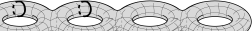
Figure 7. Graph $\Gamma_{k}(g)$ (on the left) representing $k$ pairwise non-homotopic non-separating simple closed curves on a surface of genus $g$ (on the right).

Notation $A(g,k)\preceq B(g,k)$ used in this section for asymptotic inequalities between positive quantities means that for any $\varepsilon>0$ there exists $g_{0}\in{\mathbb{N}}$ such that for all $g>g_{0}$ one has $A(g,k)\leq(1+\varepsilon)\cdot B(g,k)$ for all integer $k$ in the interval $[1;C\log(g)]$, where $C>0$ is specified separately. Notation $A(g,k)\sim B(g,k)$ is used when $\lim_{g\to+\infty}\frac{A(g,k)}{B(g,k)}=1$ uniformly for all integer $k$ in the interval $[1;C\log(g)]$, where $C>0$ is specified separately.

Theorem F.1.

For any $C<2$ the following asymptotic inequalities are valid (uniformly for all integer $k$ in the interval $[1;C\log(g)]$)

(F.1) $$c^{min}_{g-k,k}\cdot\sqrt{\frac{2}{\pi}}\cdot\left(\frac{8}{3}\right)^{4g-4}\cdot\frac{\sqrt{3g-3}}{2^{k-1}\cdot k!}\cdot Z_{k}(3g-3)\preceq\\ \preceq\operatorname{Vol}(\Gamma_{k}(g))\preceq c^{max}_{g-k,k}\cdot\sqrt{\frac{2}{\pi}}\cdot\left(\frac{8}{3}\right)^{4g-4}\cdot\frac{\sqrt{3g-3}}{2^{k-1}\cdot k!}\cdot Z_{k}(3g-3)\quad\text{as }g\to+\infty\,,$$

where $c^{max}_{g,k},c^{min}_{g,k}$ are defined in (E.6), and (E.7) respectively and $Z_{k}(3g-3)$ denotes the sum (D.25).

We first state two Corollaries of this Theorem and then prove the Theorem.

Corollary F.2.

Conjecture E.1 implies the following asymptotic expansion for any fixed $k\in{\mathbb{N}}$ as $g\to+\infty$:

(F.2) $$\operatorname{Vol}(\Gamma_{k}(g))\sim\sqrt{\frac{2}{\pi}}\cdot\left(\frac{8}{3}\right)^{4g-4}\cdot\frac{1}{\sqrt{3g-3}}\,\cdot\\ \cdot\frac{1}{2^{k-1}}\,\cdot\left(\sum_{j=0}^{k-1}\frac{B_{j}}{(k-1-j)!}\cdot\big{(}\log(3g-3)\big{)}^{k-1-j}\right)\sim\\ \sim\sqrt{\frac{2}{\pi}}\cdot\left(\frac{8}{3}\right)^{4g-4}\cdot\frac{1}{\sqrt{3g-3}}\cdot\frac{1}{(k-1)!}\cdot\left(\frac{\log(6g-6)+\gamma}{2}\right)^{k-1}\,.$$

Proof.

The first equivalence is a combination of the asymptotic expansion (D.25) from Theorem D.8 for $Z_{k}(3g-3)$ with conjectural asymptotic formula (E.8) for $c^{max}_{g,k}$ and $c^{min}_{g,k}$ from Conjecture E.1. The second equivalence corresponds to asymptotic formula (D.6) from Theorem D.3. ∎

Let $k\leq C\log(g)$. Define

(F.3) $$V_{k}(g)=\sqrt{\frac{2}{\pi}}\cdot\left(\frac{8}{3}\right)^{4g-4}\cdot\frac{\sqrt{3g-3}}{2^{k-1}\cdot k!}\cdot Z_{k}(3g-3)\ =\ \sqrt{\frac{2}{\pi}}\cdot\left(\frac{8}{3}\right)^{4g-4}\cdot\\ \cdot\frac{1}{\sqrt{3g-3}}\cdot\frac{1}{2^{k-1}}\,\cdot\left(\sum_{j=0}^{k-1}\frac{B_{j}}{(k-1-j)!}\cdot\big{(}\log(3g-3)\big{)}^{k-1-j}+\varepsilon_{k}^{Z}(3g-3)\right)\,,$$

where $\varepsilon_{k}^{Z}(m)$ is defined in (1.48) from Conjecture 1.30.

Corollary F.3.

For any $C<2$ for which Conjecture 1.28 is valid we have:

(F.4) $$\lim_{g\to+\infty}\max_{1\leq k\leq C\log(g)}\frac{V_{k}(g)}{\operatorname{Vol}(\Gamma_{k}(g))}=\lim_{g\to+\infty}\min_{1\leq k\leq C\log(g)}\frac{V_{k}(g)}{\operatorname{Vol}(\Gamma_{k}(g))}=1\,.$$

Proof.

Consider expression (F.1) from Theorem F.1. Conjecture 1.28 claims that $c^{min}_{g-k,k}$ and $c^{max}_{g-k,k}$ tend to $1$ uniformly for all $k$ in the interval $\big{[}1;[C\log(g)]\big{]}$ when $g\to+\infty$. Applying expression (1.48) for $Z_{k}(3g-3)$ we get the desired relation. ∎

Remark.

Note that at this stage we do not yet make any assertions on asymptotic behavior of $\varepsilon_{k}^{Z}(3g-3)$, so at this stage we do not rely on Conjecture 1.30.

Proof of Theorem F.1.

The automorphism group $\operatorname{Aut}(\Gamma_{k}(g))$ consists of all possible permutations of loops composed with all possible flips of individual loops, so

$$|\operatorname{Aut}(\gamma)|=2^{k}\cdot k!\,.$$

The graph $\Gamma_{k}(g)$ has single vertex, so $|V(\Gamma)|=1$. The surface does not have any marked points, so $n=0$. Thus, applying (1.14) to $\Gamma_{k}(g)$ we get

(F.5) $$\operatorname{Vol}(\Gamma_{k}(g))=\frac{2^{6g-5}\cdot(4g-4)!}{(6g-7)!}\cdot\\ \cdot 1\cdot\frac{1}{2^{k}\cdot k!}\cdot\mathcal{Z}\big{(}b_{1}b_{2}\dots b_{k}\cdot N_{g-k,2k}(b_{1},b_{1},b_{2},b_{2},\dots,b_{k},b_{k})\big{)}=\\ =\frac{(4g-4)!}{(6g-7)!}\cdot\frac{2^{6g-5}}{2^{k}\cdot k!}\cdot\frac{1}{2^{5(g-k)-6+4k}}\cdot\\ \sum_{\boldsymbol{d}\in\Pi(3g-3-k,2k)}\frac{\langle\psi^{\mathbf{d}}\rangle_{g-k,2k}}{\mathbf{d}!}\,\cdot\,\prod_{i=1}^{k}\Big{(}(2d_{2i-1}+2d_{2i}+1)!\,\cdot\,\zeta(2d_{2i-1}+2d_{2i}+2)\Big{)}\,.$$

Rewrite the latter sum using notations $\textbf{D}=(D_{1},\dots,D_{k})\in\Pi(3g-3-k,k)$ and $c_{g-k,k}(\boldsymbol{D})$ defined by (E.4). Adjusting expression (E.4) given for genus $g$ to genus $g-k$ we get

$$\sum_{\boldsymbol{d}\in\Pi(3g-3-k,2k)}\frac{\langle\psi^{\mathbf{d}}\rangle_{g-k,2k}}{\mathbf{d}!}\,\cdot\,\prod_{i=1}^{k}\Big{(}(2d_{2i-1}+2d_{2i}+1)!\,\cdot\,\zeta(2d_{2i-1}+2d_{2i}+2)\Big{)}=\\ =\sum_{\boldsymbol{D}\in\Pi(3g-3-k,2k)}c_{g-k,k}(\boldsymbol{D})\cdot\frac{(6(g-k)+4k-5)!}{(g-k)!\cdot(3(g-k)-3+2k)!}\cdot\frac{2^{3(g-k)-6+5k}}{3^{(g-k)}}\cdot\\ \cdot\prod_{j=1}^{k}\frac{\zeta(2D_{j}+2)}{2D_{j}+2}\,.$$

which allows to rewrite (F.5) as

$$\operatorname{Vol}(\Gamma_{k}(g))=\\ =\left(\frac{(4g-4)!}{(6g-7)!}\cdot 2^{g+1}\cdot\frac{1}{k!}\right)\cdot\left(\frac{(6g-2k-5)!}{(g-k)!\cdot(3g-3-k)!}\cdot\frac{2^{3g-6+2k}}{3^{(g-k)}}\right)\cdot\\ \sum_{\boldsymbol{D}\in\Pi(3g-3-k,2k)}\frac{c_{g-k,k}(\boldsymbol{D})}{2^{k}}\cdot\prod_{j=1}^{k}\frac{\zeta(2D_{j}+2)}{D_{j}+1}\,.$$

Rearranging factors with factorials and powers of $2$ and $3$, using (E.6) and (E.7) for the bounds of $c_{g-k,k}(\boldsymbol{D})$ and passing to notation (D.25) we get the following bounds:

(F.6) $$c^{min}_{g-k,k}\leq\operatorname{Vol}(\Gamma_{k}(g)):\\ \left(\frac{(6g-2k-5)!}{(6g-7)!}\cdot\frac{(4g-4)!}{(g-k)!\cdot(3g-3-k)!}\cdot\frac{2^{4g-5+3k}}{3^{(g-k)}}\cdot\frac{1}{k!}\cdot Z_{k}(3g-3)\right)\\ \leq c^{max}_{g-k,k}$$

We have the following asymptotic equivalence uniform for all $k\in[1;C\log(g)]$:

(F.7) $$\frac{(4g-4)!}{(g-k)!\cdot(3g-3-k)!}\sim\frac{(4g-4)!}{(g-1)!\cdot(3g-3)!}\cdot g^{k-1}\cdot(3g)^{k}\sim\\ \sim\sqrt{\frac{2}{\pi(3g-3)}}\cdot\left(\frac{2^{8}}{3^{3}}\right)^{g-1}\cdot 3^{k}\cdot g^{2k+1}\quad\text{as }g\to+\infty\,,$$

where in the second line we applied asymptotic formula (4.35) for the binomial coefficient $\binom{4(g-1)}{g-1}$. We also have the following asymptotic equivalence uniform for all $k\in[1;C\log(g)]$:

(F.8) $$\frac{(6g-2k-5)!}{(6g-7)!}\sim\frac{1}{(6g)^{2k-2}}\quad\text{as }g\to+\infty\,.$$

Using the two above equivalences and collecting powers of $2$, of $3$ and of $g$, we can rewrite (F.6) in the following way:

$$c^{min}_{g-k,k}\preceq\cfrac{\operatorname{Vol}(\Gamma_{k}(g))}{\sqrt{\frac{2}{\pi}}\cdot\left(\frac{8}{3}\right)^{4g-4}\cdot\frac{\sqrt{3g-3}}{2^{k-1}\cdot k!}\cdot Z_{k}(3g-3)}\preceq c^{max}_{g-k,k}\,.$$

∎

F.2. Volume contribution of stable graphs with single vertex

Conditional Theorem F.4.

Suppose that both Conjectures 1.28 and 1.30 are valid for some $C\in]\tfrac{1}{2};2[$. Then

(F.9) $$\sum_{k=1}^{[C\log(g)]}\operatorname{Vol}(\Gamma_{k}(g))\sim\frac{4}{\pi}\cdot\left(\frac{8}{3}\right)^{4g-4}\quad\text{as }g\to+\infty\,.$$

Proof.

Applying (F.4) from Corollary F.3, passing to notations (D.26) and applying (D.29) from Conditional Theorem D.9 we get

$$\sum_{k=1}^{[C\log(g)]}\operatorname{Vol}(\Gamma_{k}(g))\sim\sum_{k=1}^{[C\log(g)]}V_{k}(g)\sim\\ \sim\sqrt{\frac{2}{\pi}}\cdot\left(\frac{8}{3}\right)^{4g-4}\cdot\sqrt{3g-3}\cdot\sum_{k=1}^{[C\log(g)]}\frac{Z_{k}(3g-3)}{2^{k-1}\cdot k!}\sim\\ \sim\sqrt{\frac{2}{\pi}}\cdot\left(\frac{8}{3}\right)^{4g-4}\cdot\sqrt{3g-3}\cdot S^{\zeta}(C,3g-3)\sim\\ \sim\sqrt{\frac{2}{\pi}}\cdot\left(\frac{8}{3}\right)^{4g-4}\cdot 2\sqrt{\frac{2}{\pi}}=\frac{4}{\pi}\cdot\left(\frac{8}{3}\right)^{4g-4}\,.$$

∎

F.3. Approximation by Poisson distribution

The distribution, where

(F.10) $$p(n;\lambda)=\operatorname{Probability}(X=n)=e^{-\lambda}\cdot\frac{\lambda^{n}}{n!}\ \text{ for }n=0,1,2,\dots$$

is the Poisson distribution. It is known that the expected value and the variance of Poisson distribution are equal to $\lambda$:

$$\operatorname{E}(X)=\operatorname{Var}(X)=\lambda\,.$$

and that the Poisson distribution tends to normal distribution for large values of $\lambda$.

Recall that by $\operatorname{Vol}_{k\textit{-cyl}}(\mathcal{Q}_{g})$ we denote the contribution of square-tiled surfaced with exactly $k$ maximal horizontal cylinders to the Masur–Veech volume $\operatorname{Vol}\mathcal{Q}_{g}$. The relations

$$\sum_{k=1}^{3g-3}\operatorname{Vol}_{k\textit{-cyl}}=\operatorname{Vol}\mathcal{Q}_{g}\,,\qquad\sum_{k=1}^{\log(g)}\operatorname{Vol}(\Gamma_{k}(g))\overset{?}{\sim}\operatorname{Vol}\mathcal{Q}_{g}$$

(where the first one is an identity and the second one is conjectural) imply that the collections of positive numbers $\frac{\operatorname{Vol}(\Gamma_{k}(g))}{\operatorname{Vol}\mathcal{Q}_{g}}$ and $\frac{\operatorname{Vol}_{k\textit{-cyl}}}{\operatorname{Vol}\mathcal{Q}_{g}}$ can be interpreted as probability distributions, see Section 1.10 for details. It would be convenient to complete every such finite sequence by zeroes to work only with probability distributions indexed by indices $k\in{\mathbb{N}}$.

We study large genus asymptotics of these distributions. Conditional Theorem F.4 and Conjecture 1.10 imply that the two distributions converge in total variation, so we can restrict our considerations to the large genus asymptotics of the distribution $\frac{\operatorname{Vol}(\Gamma_{k}(g))}{\operatorname{Vol}\mathcal{Q}_{g}}$.

We study it in two regimes. In the first regime we consider the “left tail” of the distribution of a bounded length $K$. In plain terms, we consider the large genus asymptotics of the finite collection of numbers $\frac{\operatorname{Vol}(\Gamma_{1}(g))}{\operatorname{Vol}\mathcal{Q}_{g}},\dots,\frac{\operatorname{Vol}(\Gamma_{K}(g))}{\operatorname{Vol}\mathcal{Q}_{g}}$.

In the second regime we consider $k$ in the full range and let $g$ grow. We show that conditionally to our Conjectures both distributions are asymptotically well-approximated by Poisson distribution with parameter $\frac{\log(g)}{2}+const$. We evaluate the constant $const$ and show that it changes when passing from the first regime to the second.

Best approximation for the left tail of any fixed size.  In the first regime we assume that $k$ belongs to the range $k=1,\dots,K$ of any fixed size $K$. Having fixed $K$ we let $g$ grow. In this regime, we are interested only in the leading term of asymptotics of $\operatorname{Vol}(\Gamma_{k}(g))$ as $g\to+\infty$.

From now on $\gamma=0.5772...$ denotes the Euler–Mascheroni constant.

Conditional Theorem F.5.

Define

(F.11) $$V_{tail}(g)=\frac{2\cdot e^{\frac{\gamma}{2}}}{\sqrt{\pi}}\cdot\left(\frac{8}{3}\right)^{4g-4}\,.$$

Conjecture E.1 implies that the tail distribution $\frac{\operatorname{Vol}(\Gamma_{k}(g))}{V_{\mathit{tail}}(g)}$ corresponding to any fixed range $[1,K]$ of $k$ tends to the left tail of the Poisson distribution with parameter

(F.12) $$\lambda_{tail}(g)=\frac{\log(6g-6)+\gamma}{2}\,,$$

when $g\to\infty$ in the following sense:

$$\lim_{g\to+\infty}\frac{\operatorname{Vol}(\Gamma_{k}(g))}{V_{\mathit{tail}}(g)}\cdot\frac{1}{p(k-1;\lambda_{\mathit{tail}}(g))}=1\quad\text{for }k=1,\dots,K\,.$$

Note that we have to shift the index of $p(\ast;\lambda_{\mathit{tail}}(g))$ by $1$: our count starts from $k=1$, while the Poisson distribution starts from $p(0;\lambda_{\mathit{tail}}(g))$.

Proof.

Conditional to Conjecture E.1, the leading term of the volume contribution $\operatorname{Vol}(\Gamma_{k}(g))$ is given by the last line in (F.2) in Corollary F.2. Thus,

$$\frac{\operatorname{Vol}(\Gamma_{k}(g))}{V_{\mathit{tail}}(g)}\sim\frac{1}{\sqrt{2}\cdot e^{\frac{\gamma}{2}}}\cdot\frac{1}{\sqrt{3g-3}}\cdot\frac{1}{(k-1)!}\left(\frac{\log(6g-6)+\gamma}{2}\right)^{k-1}\!\!\!=\frac{1}{e^{\lambda_{\mathit{tail}}}}\cdot\frac{\lambda_{\mathit{tail}}^{k-1}}{(k-1)!}\,.$$

∎

Best approximation near maximal values.  Let us study now the large genus asymptotics of the distribution $\frac{\operatorname{Vol}(\Gamma_{k}(g))}{\operatorname{Vol}\mathcal{Q}_{g}}$ in the full range range of $k$. We transform finite collections of numbers into sequences completing any finite collection by infinite sequence of zeroes. Speaking of convergence of sequences we always mean the $\ell^{1}$-convergence (equivalently, convergence in total variation). Using technical Lemma F.6 we prove in Lemma F.7 that certain convenient auxiliary sequence $\{v_{k}(g)\}_{k\in{\mathbb{N}}}$ defined below converges to the Poisson distribution. Finally, we prove in Conditional Theorem F.8 that the sequence $\{v_{k}(g)\}$ converges to $\{\frac{\operatorname{Vol}(\Gamma_{k}(g))}{\operatorname{Vol}\mathcal{Q}_{g}}\}$ and that the latter sequence converges to the sequence $\left\{\frac{\operatorname{Vol}_{k\textit{-cyl}}\mathcal{Q}_{g}}{\operatorname{Vol}\mathcal{Q}_{g}}\right\}$.

Define the following function $c(x)$ on the interval $C\in[0;2]$:

(F.13) $$c(C)=\begin{cases}\frac{1}{C-\tfrac{1}{2}}\cdot\left(\frac{\log(\pi)-3\log(2)}{2}+C\log(2)-\log\Gamma(1+C)\right)\,,&\text{when }C\neq\tfrac{1}{2}\,,\\ 3\log(2)+\gamma-2\,,&\text{when }C=\tfrac{1}{2}\,.\end{cases}$$

Note that

$$\lim_{C\to\tfrac{1}{2}}c(C)=\left(\frac{\log(\pi)-3\log(2)}{2}+C\log(2)-\log\Gamma(1+C)\right)^{\prime}\Big{|}_{C=\tfrac{1}{2}}=\\ =\log(2)-\psi\left(\tfrac{3}{2}\right)=\log(2)-(-\gamma-2\log(2)+2)=3\log(2)+\gamma-2\,,$$

where we used (D.38) for the value $\psi\left(\tfrac{3}{2}\right)$. Thus, the function $c$ is continuous on the interval $[0;2]$. It is monotonously decreasing on this interval from $c(0)=3\log(2)-\log(\pi)\approx 0.934712$ to $c(2)=\frac{1}{3}(\log(\pi)-\log(2))\approx 0.150528$.

Lemma F.6.

Suppose that for some $C\in]0;2[$ Conjectures 1.28 and 1.30 are valid. Let

(F.14) $$v_{k}(g)=\sqrt{\frac{\pi}{8}}\cdot\frac{1}{\sqrt{3g-3}}\,\cdot\frac{1}{2^{k-1}}\,\cdot\left(\sum_{j=0}^{k-1}\frac{B_{j}}{(k-1-j)!}\cdot\big{(}\log(3g-3)\big{)}^{k-1-j}\right)$$

for $k=1,\dots,[C\log(g)]$ and let $v_{k}(g)=0$ for $k>[C\log(g)]$. Let

(F.15) $$\lambda(C)=\frac{\log(3g-3)+c(C)}{2}\,,$$

and let $K(C,g)=[C\log(3g-3)]$. Then

(F.16) $$\lim_{g\to+\infty}\frac{v_{K(C,g)}(g)}{p(K(C,g)-1;\lambda(C))}=1\,,$$

where $p(n,\lambda)$ is defined in (F.10).

Proof.

Plugging the definition (F.15) of $\lambda(C)$ into the definition (F.10) of $p(K-1,\lambda)$ we get

$$p(K-1;\lambda)=\frac{e^{-\tfrac{c}{2}}}{\sqrt{3g-3}}\cdot\frac{(\log(3g-3)+c)^{K-1}}{(K-1)!\cdot 2^{K-1}}\,,$$

where $K=K(C,g)$ and $c=c(C)$. Thus, proving (F.16) is equivalent to proving the following relation:

$$\lim_{g\to+\infty}\frac{(K-1)!}{(\log(3g-3)+c)^{K-1}}\cdot\left(\sum_{j=0}^{K-1}\frac{B_{j}}{(K-1-j)!}\cdot\big{(}\log(3g-3)\big{)}^{K-1-j}\right)\overset{?}{=}\frac{e^{-\tfrac{c}{2}}}{\sqrt{\tfrac{\pi}{8}}}\,,$$

where, for brevity, we denote $K=K(C,g)$ and $c=c(C)$. We can rewrite the expression in the left-hand side of the above relation as

$$B_{0}\cdot\left(\frac{\log(3g-3)}{\log(3g-3)+c}\right)^{K-1}+B_{1}\cdot\frac{(K-1)}{\big{(}\log(3g-3)+c\big{)}}\cdot\left(\frac{\log(3g-3)}{\log(3g-3)+c}\right)^{K-2}+\\ +B_{2}\frac{(K-1)(K-2)}{\big{(}\log(3g-3)+c\big{)}^{2}}\left(\frac{\log(3g-3)}{\log(3g-3)+c}\right)^{K-3}\!\!\!\!+\dots+B_{K-1}\frac{(K-1)!}{\big{(}\log(3g-3)+c\big{)}^{K-1}}\,.$$

We have seen that $c(C)\in]0;1[$ for any $C\in]0;2[$. Thus, for any fixed $n$ we get

$$\left(\frac{K-n}{\log(3g-3)+c}\right)\sim C\quad\text{as }g\to+\infty\,,$$

and

$$\left(\frac{\log(3g-3)}{\log(3g-3)+c}\right)^{K-n}\sim\left(1-\frac{c}{\log(3g-3)}\right)^{[C\log(3g-3)]}\sim e^{-c\cdot C}\quad\text{as }g\to+\infty\,.$$

Hence, for any fixed $n\in{\mathbb{N}}$, we get the following asymptotic expression for the first $n+1$ terms of the above sum:

$$B_{0}\cdot\left(\frac{\log(3g-3)}{\log(3g-3)+c}\right)^{K-1}+B_{1}\cdot\frac{(K-1)}{\big{(}\log(3g-3)+c\big{)}}\cdot\left(\frac{\log(3g-3)}{\log(3g-3)+c}\right)^{K-2}+\dots{\\ }+\dots+B_{n}\cdot\frac{(K-1)\dots(K-n)}{\big{(}\log(3g-3)+c\big{)}^{n}}\cdot\left(\frac{\log(3g-3)}{\log(3g-3)+c}\right)^{K-n+1}\sim\\ \sim e^{-c\cdot C}\cdot\left(B_{0}+B_{1}\cdot C+B_{2}\cdot C^{2}+\dots+B_{n}\cdot C^{n}\right)\quad\text{as }g\to+\infty\,.$$

The absolute value of the remaining part of the sum is trivially bounded from above by

$$\sum_{j=n+1}^{+\infty}|B_{j}|\cdot C^{j}\,.$$

By (D.19) the latter expression rapidly converges to $0$ as $n$ grows. Hence the desired relation (F.16) is equivalent to the following relation

$$\frac{e^{-\tfrac{c}{2}}}{\sqrt{\tfrac{\pi}{8}}}\overset{?}{=}e^{-c\cdot C}\cdot\sum_{j=0}^{+\infty}B_{j}\cdot C^{j}\,.$$

Applying (D.16) for the sum on the right-hand side we can rewrite the latter equation as:

$$e^{c\cdot(C-\tfrac{1}{2})}\overset{?}{=}\sqrt{\tfrac{\pi}{8}}\cdot\frac{2^{C}}{\Gamma(1+C)}\,.$$

Note that

$$\Gamma\left(1+\tfrac{1}{2}\right)=\frac{\sqrt{\pi}}{2}$$

so for $C=\tfrac{1}{2}$ the relation is satisfied. Suppose now that $C\neq\tfrac{1}{2}$. The above equation implicitly defines $c$ as a function of $C$. Taking logarithms of both sides and dividing the resulting expression by $(C-\frac{1}{2})$ we get exactly the expression for $c(C)$ from (F.13). Lemma F.6 is proved. ∎

Lemma F.7.

Suppose that both Conjectures 1.28 and 1.30 are valid for some $C$ in the interval $]\frac{1}{2};2[$. Then, the sequence $\{v_{k}(g)\}_{k\in{\mathbb{N}}}$ converges in total variation to the Poisson distribution $\{p(k-1,\lambda)\}_{k\in{\mathbb{N}}}$ with parameter

$$\lambda(g)=\frac{\log(6g-6)+\gamma}{2}+(\log 2-1)\,,$$

when $g\to\infty$.

Proof.

Choose any $\varepsilon$ satisfying $0<\varepsilon\ll\frac{1}{2}$ and any $M\gg 1$. Consider the following subsets of ${\mathbb{N}}$:

$$I_{1} =\{1,2,\dots,[\varepsilon\log(g)]\}\,,$$

$$I_{2} =\left\{[\varepsilon\log(g)]+1,[\varepsilon\log(g)]+2,\dots,[\lambda(g)-M\sqrt{\log(g)}]\right\}\,,$$

$$I_{3} =\left\{[\lambda(g)-M\sqrt{\log(g)}],\dots,[\lambda(g)+M\sqrt{\log(g)}]\right\}\,,$$

$$I_{4} =\left\{[\lambda(g)+M\sqrt{\log(g)}]+1,[\lambda(g)+M\sqrt{\log(g)}]+2,\dots,[C\log(g)]\right\}\,,$$

$$I_{5} =\big{\{}[C\log(g)]+1,[C\log(g)]+2,\dots\big{\}}\,.$$

We assume that $g$ is sufficiently large so that all these intervals are nonempty. We bound the sum $\sum|v_{k}(g)-p(k-1,\lambda(g))|$ from above separately on each of these intervals.

The contributions of the left tails of both sequences tend to zero as $g\to+\infty$:

$$\lim_{g\to+\infty}\sum_{k\in I_{1}}v_{k}=\lim_{g\to+\infty}\sum_{k\in I_{1}}p(k-1,\lambda(g))=0\,,$$

so

$$\lim_{g\to+\infty}\sum_{k\in I_{1}}|v_{k}-p(k-1,\lambda(g))|=0\,.$$

Choosing $M$ sufficiently large, we can make the contribution

$$\lim_{g\to+\infty}\sum_{k\in I_{2}\sqcup I_{4}}p(k-1,\lambda(g))$$

arbitrary small. It follows from Lemma F.6 that for all sufficiently large $g$ we have

$$v_{k}(g)\leq T\cdot p(k-1,\lambda(g))\quad\text{for }k\in I_{2}\sqcup I_{4}\,,$$

with universal constant $T$ depending only on $\varepsilon$. Thus, choosing $M$ sufficiently large, we can make the variation

$$\lim_{g\to+\infty}\sum_{k\in I_{2}\sqcup I_{4}}|v_{k}(g)-p(k-1,\lambda(g))|$$

on these two intervals arbitrary small.

For any fixed $M$ the ratio $\frac{v_{k}(g)}{p(k-1,\lambda(g))}$ tends to $1$ uniformly for all $k\in I_{3}$. Thus, we get

$$\lim_{g\to+\infty}\sum_{k\in I_{3}}|v_{k}(g)-p(k-1,\lambda(g))|=0\,.$$

Finally

$$\lim_{g\to+\infty}\sum_{k\in I_{5}}|v_{k}(g)-p(k-1,\lambda(g))|=\lim_{g\to+\infty}\sum_{k\in I_{5}}|p(k-1,\lambda(g))|=0\,.$$

which completes the proof of Lemma F.7. ∎

Conditional Theorem F.8.

Conjectures 1.10, 1.28, 1.30 together imply that the distribution

$$\frac{\operatorname{Vol}_{1\textit{-cyl}}\mathcal{Q}_{g}}{\operatorname{Vol}\mathcal{Q}_{g}},\dots,\frac{\operatorname{Vol}_{(3g-3)\textit{-cyl}}\mathcal{Q}_{g}}{\operatorname{Vol}\mathcal{Q}_{g}}$$

tends to Poisson distribution $p(k-1,\lambda(g))$ with parameter

(F.17) $$\lambda(g)=\frac{\log(6g-6)+\gamma}{2}+(\log 2-1)\,,$$

when $g\to\infty$. Note that we have to shift indices by $1$: our count starts from $k=1$, while the Poisson distribution starts from $n=0$.

Proof.

Let

$$V(g)=\frac{4}{\pi}\cdot\left(\frac{8}{3}\right)^{4g-4}\,.$$

By Conjecture 1.10 and by (F.9) in Conditional Theorem F.4 we have

$$\operatorname{Vol}\mathcal{Q}_{g}\sim V(g)\sim\sum_{k=1}^{[C\log(g)]}\operatorname{Vol}(\Gamma_{k}(g))\quad\text{ as }g\to+\infty\,.$$

Since $\operatorname{Vol}_{k\textit{-cyl}}\mathcal{Q}_{g}\geq\operatorname{Vol}(\Gamma_{k}(g))\geq 0$ for all $k$, this implies $\ell^{1}$-convergence of the sequences

(F.18) $$\left(\frac{\operatorname{Vol}_{1\textit{-cyl}}}{\operatorname{Vol}\mathcal{Q}_{g}},\frac{\operatorname{Vol}_{2\textit{-cyl}}}{\operatorname{Vol}\mathcal{Q}_{g}},\dots,\frac{\operatorname{Vol}_{(3g-3)\textit{-cyl}}}{\operatorname{Vol}\mathcal{Q}_{g}},0,0,\dots\right)\to\\ \to\left(\frac{\operatorname{Vol}(\Gamma_{1}(g))}{V(g)},\frac{\operatorname{Vol}(\Gamma_{2}(g))}{V(g)},\dots,\frac{\operatorname{Vol}(\Gamma_{[C\log(g)]}(g))}{V(g)},0,0,\dots\right)\quad\text{as }g\to+\infty\,.$$

Equation (F.4) from Corollary F.3 implies uniform convergence and, hence, $\ell^{1}$-convergence of the following sequences:

(F.19) $$\left(\frac{\operatorname{Vol}(\Gamma_{1}(g))}{V(g)},\frac{\operatorname{Vol}(\Gamma_{2}(g))}{V(g)},\dots,\frac{\operatorname{Vol}(\Gamma_{[C\log(g)]}(g))}{V(g)},0,0,\dots\right)\to\\ \to\left(\frac{V_{1}(g)}{V(g)},\frac{V_{2}(g)}{V(g)},\dots,\frac{V_{[C\log(g)]}(g)}{V(g)},0,0,\dots\right)\quad\text{as }g\to+\infty\,.$$

where $V_{k}(g)$ is defined in (F.3).

Equation (1.50) from Conjecture 1.30 claims $\ell^{1}$-convergence

(F.20) $$\left\{\frac{\operatorname{Vol}(\Gamma_{k}(g))}{V}\right\}_{k\in{\mathbb{N}}}\to\{v_{k}(g)\}_{k\in{\mathbb{N}}}\quad\text{ as }g\to+\infty\,.$$

Convergence of $\{v_{k}(g)\}$ to the Poisson distribution with parameter $\lambda(g)$ is proved in Lemma F.7. ∎

Remark F.9.

Note that the parameter $\lambda_{tail}$ which provides the best approximation by the Poisson distribution for the left tail of the the distribution of any fixed finite size differs from the parameter $\lambda$ which provides the best approximation by the Poisson distribution globally for the entire distribution $\frac{\operatorname{Vol}_{k\textit{-cyl}}\mathcal{Q}_{g}}{\operatorname{Vol}\mathcal{Q}_{g}}$, where $k=1,\dots,3g-3$. Comparing (F.12) and (F.17) we get

$$\lambda(g)=\lambda_{tail}(g)+(\log 2-1)\approx\lambda_{tail}(g)-0.306853\,.$$

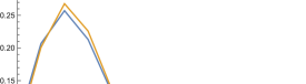
Figure 8. Experimental distribution of contribution of $k$-cylinder surfaces (in orange) and the Poisson distribution with $\lambda$ as in (F.17) (in blue)

Figure 8 presents the graph of the experimental statistics of frequencies of $k$-cylinder surfaces in $g=26$ and the Poisson distribution with parameter $\lambda$ evaluated by (F.17). We joined the neighboring points of the discrete graph by segments for better visibility. The experimental statistics has slightly higher maximum compared to Poisson distribution and its left slope is shifted a little bit to the right compared to the Poisson distribution. Already for $g=26$ we observe that we would get slightly better approximation of the left tail of the experimental statistics by Poisson distribution choosing $\lambda(26)$ slighly larger. However, the optimal approximation of the experimental data by all possible Poisson distribution gives

$$\lambda_{\textit{optimal}}(26)\approx 2.528\,,$$

so the parameter $\lambda(26)\approx 2.487$ calculated using (F.17) and used for the graph in Figure 8 provides much better fit than $\lambda_{tail}(26)\approx 2.794$ given by (F.12).

F.4. Numerical evidence

We have two independent sources of numerical evidence for our Conjectures. The first source is exact computation of all $\operatorname{Vol}\Gamma_{k}(g)$ for $g\leq 9$. Table 6 provides the rational coefficients $\frac{p}{q}$ in the contribution $\frac{p}{q}\cdot\pi^{6g-6}$ of $\operatorname{Vol}(\Gamma_{k}(g))$ to $\operatorname{Vol}\mathcal{Q}(1^{4g-4})$. We have all exact values of analogous quantities for $g\leq 9$.

$${\begin{array}[]{|c|c|c|c|c|}\hline\cr&&&&\\[-6.0pt] g&k=1&k=2&k=3&k=4\\ &&&&\\[-6.0pt] \hline\cr&&&&\\[-6.0pt] 2&\frac{16}{945}&\frac{8}{225}&&\\ &&&&\\[-6.0pt] \hline\cr&&&&\\[-6.0pt] 3&\frac{204536}{273648375}&\frac{2206912}{1620840375}&\frac{2704}{3189375}&\\ &&&&\\[-6.0pt] \hline\cr&&&&\\[-6.0pt] 4&\frac{80320477}{2362381544250}&\frac{16548755563}{251883751494375}&\frac{18410248}{368225463375}&\frac{16128416}{987779417625}\\ &&&&\\[-6.0pt] \hline\cr&&&&\\[-6.0pt] 5&\frac{10303583454872}{6451867979907013125}&\frac{19854998108336976488}{6136611136849420367765625}&\frac{2276745597432209408}{827792583677569525640625}&\frac{1412757290717388688}{1158909617148597335896875}\\ &&&&\\ \hline\cr\end{array}}$$

Table 6. Exact values of $\cfrac{\operatorname{Vol}(\Gamma_{k}(g))}{\pi^{6g-6}}$

We have also explicitly computed $\operatorname{Vol}\mathcal{Q}_{g}$ for $g=2,\dots,6$, see Table 5. Table 7 gives the following approximate values of the ratios $\cfrac{\sum_{k=1}^{g}\operatorname{Vol}(\Gamma_{k}(g))}{\operatorname{Vol}\mathcal{Q}(1^{4g-4})}$ for these genera:

$$\begin{array}[]{|c|c|c|c|c|}\hline\cr&&&&\\[-6.0pt] g=2&g=3&g=4&g=5&g=6\\ &&&&\\[-6.0pt] \hline\cr&&&&\\[-6.0pt] 0.787&0.855&0.909&0.940&0.959\\[-6.0pt] &&&&\\ \hline\cr\end{array}$$

Table 7. Approximate values of $\cfrac{\sum_{k=1}^{g}\operatorname{Vol}(\Gamma_{k}(g))}{\operatorname{Vol}\mathcal{Q}(1^{4g-4})}$.

One can argue that genus $6$ is still a bit far from infinity. However, $\dim_{{\mathbb{C}}}\mathcal{Q}_{6}=30$ and in the case of Abelian differentials, the Masur–Veech volumes of all strata are already quite close to their asymptotic values for this range of dimensions.

Another source of numerical evidence is the following experimental data. We can quite efficiently collect experimental statistics $\cfrac{\operatorname{Vol}_{k\textit{-cyl}}\mathcal{Q}_{g}}{\operatorname{Vol}\mathcal{Q}_{g}}$ of the number $k=1,\dots,3g-3$ of maximal horizontal cylinders in a “random” square-tiled surface in $\mathcal{Q}_{g}$. We compare it to statistics $\cfrac{v_{k}(g)}{V(g)}$. The resulting normalized probability distributions for $g=26$ are presented at Figure 9.

Recall that for $k=1$ and for sufficiently large genus, $\operatorname{Vol}\Gamma_{1}(g)$ gives practically all contribution of $1$-cylinder square-tiled surfaces to $\operatorname{Vol}\mathcal{Q}_{g}$, that is

$$\frac{\operatorname{Vol}\Gamma_{1}(g)}{\operatorname{Vol}_{1\textit{-cyl}}\mathcal{Q}_{g}}\sim 1-\sqrt{\frac{2}{3\pi g}}\cdot\frac{1}{4^{g}}\quad\text{as }g\to+\infty\,.$$

On the other hand, for $g=26$ the experimental value of the first term of statistics is still reasonably large, namely

$$\frac{\operatorname{Vol}_{1\textit{-cyl}}\mathcal{Q}_{26}}{\operatorname{Vol}\mathcal{Q}_{26}}\approx 0.071\,.$$

This implies that the two distributions are still reasonably close before normalizing the total mass to $1$.

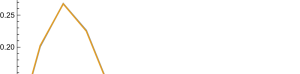
Figure 9. Experimental distribution of frequencies of $k$-cylinder square-tiled surfaces and the normalized distribution given by expression (F.2) for $\operatorname{Vol}\Gamma_{k}(g)$ in genus $g=26$

.

The experimental numerical data for frequencies of $k$-cylinder square-tiled surfaces and the normalized distribution given by expression (F.2) for $\operatorname{Vol}\Gamma_{k}(g)$ given below for genus $g=26$,

$$0.0713,0.2009,0.2679,0.2260,0.1369,0.0634,0.0237,0.0073,\dots$$

$$0.0724,0.2022,0.2675,0.2251,0.1361,0.0633,0.0237,0.0073,\dots$$

are already, basically, indistinguishable graphically, see Figure 9 (where we joined the neighboring points of the discrete graph by segments for better visibility).

References

- [Ag1] A. Aggarwal, Large Genus Asymptotics for Volumes of Strata of Abelian Differentials, arXiv:1804.05431.
- [Ag2] A. Aggarwal, Large Genus Asymptotics for Siegel–Veech Constants, to appear in GAFA, arXiv:1810.05227.
- [ABCD] J. E. Andersen, G. Borot, S. Charbonniery, V. Delecroix, A. Giacchetto, D. Lewański, C. Wheeler, Topological recursion for Masur–Veech volumes, arXiv:1905.10352.
- [ArCo] E. Arbarello, M. Cornalba, Combinatorial and algebro-geometric cohomology classes on the moduli spaces of curves, J. Algebraic Geom. 5:4 (1996), 705–749.
- [AEZ1] J. Athreya, A. Eskin, and A. Zorich, Counting generalized Jenkins–Strebel differentials, Geometriae Dedicata, 170:1 (2014), 195–217.
- [AH] F. Arana–Herrera, Counting square-tiled surfaces with prescribed real and imaginary foliations and connections to Mirzakhani’s asymptotics for simple closed hyperbolic geodesics, arXiv:1902.05626.
- [AEZ2] J. Athreya, A. Eskin, and A. Zorich, Right-angled billiards and volumes of moduli spaces of quadratic differentials on , Ann. Scient. ENS, 4ème série, 49 (2016), 1307–1381.
- [BoSö] F. Bonahon, Y. Sözen, The Weil–Petersson and Thurston Symplectic forms, Duke Math. J. 108 (2001), no. 3, 581–597.
- [ChMuSa] K. Chapman, M. Mulase, B. Safnuk, The Kontsevich constants for the volume of the moduli of curves and topological recursion, Commun. in Number Theory and Phys. 5 (2011), no. 3, 643–698.
- [C] D. Chen, Square-tiled surfaces and rigid curves on moduli spaces, Advances in Mathematics, 228 (2011), 1135–1162.
- [CMöZa] D. Chen, M. Möller, D. Zagier, Quasimodularity and large genus limits of Siegel–Veech constants, J. Amer. Math. Soc. 31 (2018), no. 4, 1059–1163.
- [CMöSZa] D. Chen, M. Möller, A. Sauvaget, D. Zagier, Masur–Veech volumes and intersection theory on moduli spaces of abelian differentials; arXiv:1901.01785.
- [DGZZ1] V. Delecroix, E. Goujard, P. Zograf, A. Zorich, Square-tiled surfaces of fixed combinatorial type: equidistribution, counting, volumes of the ambiant strata, arXiv:1612.08374 (2016) 60pp.
- [DGZZ2] V. Delecroix, E. Goujard, P. Zograf, A. Zorich, Enumeration of meanders and Masur-Veech volumes, arXiv:1705.05190.
- [DGZZ3] V. Delecroix, E. Goujard, P. Zograf, A. Zorich, with appendix of Ph. Engel, Contribution of one-cylinder square-tiled surfaces to Masur–Veech volumes, arXiv:1903.10904, to appear in Asterisque.
- [DLMF] NIST Digital Library of Mathematical Functions. F. W. J. Olver, A. B. Olde Daalhuis, D. W. Lozier, B. I. Schneider, R. F. Boisvert, C. W. Clark, B. R. Miller, and B. V. Saunders, eds., http://dlmf.nist.gov/, Release 1.0.22 of 2019-03-15.
- [En1] Ph. Engel, Hurwitz Theory of Elliptic Orbifolds, I, arXiv:1706.06738.
- [En2] Ph. Engel, Hurwitz Theory of Elliptic Orbifolds, II, arXiv::1809.07434.
- [EMa] A. Eskin, H. Masur, Asymptotic formulas on flat surfaces, Ergodic Theory and Dynamical Systems, 21 (2) (2001), 443–478.
- [EKoZo] A. Eskin, M. Kontsevich, A. Zorich, Sum of Lyapunov exponents of the Hodge bundle with respect to the Teichmüller geodesic flow, Publications de l’IHES, 120:1 (2014), 207–333.
- [EMaZo] A. Eskin, H. Masur, A. Zorich, Moduli spaces of Abelian differentials: the principal boundary, counting problems and the Siegel–Veech constants, Publications Mathématiques de l’IHES, 97 (1) (2003), 61–179.
- [EMiMo] A. Eskin, M. Mirzakhani, A. Mohammadi, Effective counting of simple closed geodesics on hyperbolic surfaces, arXiv:1905.04435.
- [EO1] A. Eskin, A. Okounkov. Asymptotics of numbers of branched coverings of a torus and volumes of moduli spaces of holomorphic differentials, Invent. Math. 145 (2001), no. 1, 59–103.
- [EO2] A. Eskin, A. Okounkov. Pillowcases and quasimodular forms, Algebraic Geometry and Number Theory, Progress in Mathematics 253 (2006), 1–25.
- [EOP] A. Eskin, A. Okounkov, R. Pandharipande, The theta characteristic of a branched covering, Adv. Math., 217 no. 3 (2008), 873–888.
- [EZo] A. Eskin, A. Zorich, Volumes of strata of Abelian differentials and Siegel–Veech constants in large genera, Arnold Mathematical Journal, 1:4 (2015), 481–488.
- [FS] Ph. Flajolet, R. Sedgewick, Analytic Combinatorics. Cambridge University Press, 2009.
- [H] J. Havil, Gamma: Exploring Euler’s Constant. Princeton, NJ: Princeton University Press, 2003.
- [G1] E. Goujard, Siegel–Veech constants for strata of moduli spaces of quadratic differentials, GAFA, 25:5 (2015), 1440–1492.
- [G2] E. Goujard, Volumes of strata of moduli spaces of quadratic differentials: getting explicit values, Ann. Inst. Fourier, 66 no. 6 (2016), 2203–2251.
- [Kon] M. Kontsevich, Intersection theory on the moduli space of curves and the matrix Airy function, Comm. Math. Phys. 147 (1992), 1–23.
- [Lag] J. Lagarias, Euler’s constant: Euler’s work and modern developments Bull. Amer. Math. Soc. 50 (2013), no. 4, 527–628.
- [Lan] E. Lanneau, Parity of the spin structure defined by a quadratic differential, Geometry and Topology 8, (2004) 511–538.
- [Ma1] H. Masur, Interval exchange transformations and measured foliations, Ann. of Math., 115 (1982), 169–200.
- [Ma2] H. Masur, The Teichmüller Flow is Hamiltonian, Proceedings of the AMS 123, No. 12 (1995), 3739–3747.
- [Mi1] M. Mirzakhani, Simple geodesics and Weil-Petersson volumes of moduli spaces of bordered Riemann surfaces, Invent. Math. 167 (2007), no. 1, 179–222.
- [Mi2] M. Mirzakhani, Weil–Petersson volumes and intersection theory on the moduli space of curves, Journal of Amer. Math. Soc. 20 (2007), no. 1, 1–23.
- [Mi3] M. Mirzakhani, Growth of the number of simple closed geodesics on hyperbolic surfaces, Annals of Math. (2) 168 (2008), no. 1, 97–125.
- [Mi4] M. Mirzakhani, Ergodic theory of the earthquake flow, IMRN 3 (2008), 1–39.
- [Mi5] M. Mirzakhani, Counting mapping class group orbits on hyperbolic surfaces, (2016) arXiv:1601.03342.
- [MiZog] M. Mirzakhani, P. Zograf, Towards large genus asymtotics of intersection numbers on moduli spaces of curves, GAFA 25 (2015), 1258–1289.
- [MoT] L. Monin, V. Telpukhovskiy, On normalizations of Thurston measure on the space of measured laminations, arXiv:1902.04533.
- [Nb] P. Norbury, Counting lattice points in the moduli space of curves, Math. Res. Lett. 17 (2010), no. 3, 467–481.
- [OP] A. Okounkov and R. Pandharipande, Gromov–Witten theory, Hurwitz theory, and matrix models, Algebraic geometry — Seattle 2005. Part 1, 325–414, Proc. Sympos. Pure Math., 80, Part 1, Amer. Math. Soc., Providence, RI, 2009.
- [RS] K. Rafi, J. Souto, Geodesics Currents and Counting Problems, arXiv:1709.06834.
- [S1] A. Sauvaget, Volumes and Siegel–Veech constants of and Hodge integrals, arXiv:1801.01744.
- [S2] A. Sauvaget, The Large genus asymptotic expansion of Masur-Veech volumes, (2019) arXiv:1903.04454.
- [Va] R. Vakil, The Moduli Space of Curves and Its Tautological Ring, Notices of the AMS (2003), 50:6, 647–658.
- [Ve1] W. Veech, Gauss measures for transformations on the space of interval exchange maps, Annals of Math., 115 (1982), 201–242.
- [Ve2] W. A. Veech, Siegel measures, Annals of Math., 148 (1998), 895–944.
- [Vo] Ya. Vorobets, Periodic geodesics on generic translation surfaces. In: “Algebraic and Topological Dynamics”, S. Kolyada, Yu. I. Manin and T. Ward (Editors), Contemporary Math., Vol. 385, Amer. Math. Soc., Providence, RI, 205–258 (2005)
- [Wi] E. Witten, Two-dimensional gravity and intersection theory on moduli space, in Surveys in differential geometry (Cambridge, MA, 1990), 243–310, Lehigh Univ., Bethlehem, PA, 1991
- [Zog] P. Zograf, An explicit formula for Witten’s -correlators, Zap. Nauchn. Sem. S.-Peterburg. Otdel. Mat. Inst. Steklov. (POMI) 468 (2018), 53–57.
- [Zor] A. Zorich, Square tiled surfaces and Teichmüller volumes of the moduli spaces of abelian differentials. Rigidity in dynamics and geometry (Cambridge, 2000), 459–471, Springer, Berlin, 2002.