Abstract

Interlocus gene conversion (IGC) homogenizes paralogs. Little is known regarding the mutation events that cause IGC and even less is known about the IGC mutations that experience fixation. To disentangle the rates of fixed IGC mutations from the tract lengths of these fixed mutations, we employ a composite likelihood procedure. We characterize the procedure with simulations. We apply the procedure to duplicated primate introns and to protein-coding paralogs from both yeast and primates. Our estimates from protein-coding data concerning the mean length of fixed IGC tracts were unexpectedly low and are associated with high degrees of uncertainty. In contrast, our estimates from the primate intron data had lengths in the general range expected from IGC mutation studies. While it is challenging to separate the rate at which fixed IGC mutations initiate from the average number of nucleotide positions that these IGC events affect, all of our analyses indicate that IGC is responsible for a substantial proportion of evolutionary change in duplicated regions. Our results suggest that IGC should be considered whenever the evolution of multigene families is examined.

Article (Methods)

A phylogenetic approach disentangles interlocus gene conversion tract length and initiation rate

Keywords: interlocus gene conversion, multigene family evolution, tract length

1 Introduction

Interlocus gene conversion (IGC) homogenizes repeats by copying a tract of sequence from one paralog to the equivalent region of another. This means that evidence of nucleotide substitution in one paralog can be erased and that the ancestry of an IGC tract coalesces in two paralogs when IGC events occur. As a result, IGC events partition the sequence sites of a multigene family into regions that have different evolutionary trees. This consequence of IGC has complicated the study of multigene family evolution, especially when the goals are to examine orthology and the history of gene duplication and loss. Incorporating tract length into IGC inference can therefore be helpful for disentangling the local correlation structure of the histories of sequence sites.

In Ji et al. (2016), we introduced an approach to incorporate IGC into any existing nucleotide substitution model by jointly considering the corresponding nucleotide or codon sites in different paralogs. One limitation of this modeling framework is that it assumes IGC events are independently experienced by sites within a paralog. The framework does not reflect the correlation structure among sites within a paralog that is induced by IGC and we will refer to it as the independent-site (IS) approach. Here, we extend the IS model by incorporating IGC tract information and introduce an accompanying inference procedure. We then illustrate the extensions of our IS approach by applying them to three diverse groups of data sets and by analyzing simulated data.

2 New Approach

The IS model can incorporate IGC by adding one new parameter ($\tau$) to any conventional substitution model that has changes originate with point mutation. The purpose of the additional parameter is to represent the homogenization among paralogs caused by IGC. For example, the HKY model (Hasegawa et al., 1985) describes nucleotide substitutions that originate with point mutation and has substitution rates depend on the type of nucleotide being introduced and whether the substitution is a transition or a transversion. The HKY rate from nucleotide type $i$ to type $i^{\prime}$ ($i\neq i^{\prime}$) is $Q_{ii^{\prime}}$ with

$${Q_{ii^{\prime}}}\propto\left\{{\begin{array}[]{*{20}{c}}{{\pi_{i^{\prime}}}}&{{\mbox{if transversion}}}\\ {\kappa{\pi_{i^{\prime}}}}&{{\mbox{if transition}}},\end{array}}\right.$$ (1)

where $\pi_{i^{\prime}}$ is the stationary probability of nucleotide type $i^{\prime}$ ($\pi_{A}+\pi_{C}+\pi_{G}+\pi_{T}=1$) and $\kappa\geq 0$ differentiates transitions and transversions. With two paralogs per genome, the IS extension of the HKY model has $Q_{(i,j),(i^{\prime},j^{\prime})}$ be the instantaneous rate at which one paralog changes from state $i$ to $i^{\prime}$ and the corresponding site of the other paralog changes from state $j$ to $j^{\prime}$. The resulting rates for possible changes are:

$${Q_{(i,j),(i^{\prime},j^{\prime})}}\propto\left\{{\begin{array}[]{*{20}{c}}0&{i\neq i^{\prime},j\neq j^{\prime}}\\ Q_{ii^{\prime}}&{i\neq i^{\prime},j=j^{\prime},i^{\prime}\neq j^{\prime}}\\ Q_{ii^{\prime}}+\tau&{i\neq i^{\prime},j=j^{\prime},i^{\prime}=j^{\prime}}\\ Q_{jj^{\prime}}&{i=i^{\prime},j\neq j^{\prime},i^{\prime}\neq j^{\prime}}\\ Q_{jj^{\prime}}+\tau&{i=i^{\prime},j\neq j^{\prime},i^{\prime}=j^{\prime}}.\end{array}}\right.$$ (2)

IGC extensions to other conventional nucleotide or codon substitution models can be made in a similar fashion.

While the IS approach considers dependence due to IGC at corresponding sites in different paralogs, it assumes IGC occurs independently at different sites within the same paralog. As Nasrallah et al. (2010) noted, the assumption of evolutionary independence among sites can be biologically unreasonable, but is often kept for simplicity and computational tractability. Ideally, dependent evolution among sequence positions would be modeled by treating entire sequences as the state of a system (e.g., Robinson et al. 2003). Having the state space consist of all possible sequences would lead to more realistic Markov models for describing how individual IGC events can affect multiple sites within a paralog. However, the size of the state space becomes large when it matches the number of possible sequences. This large size would not prove computationally tractable if employing the inference strategy outlined in Ji et al. (2016).

As a compromise between computational feasibility and realism, our new approach extends the IS model by jointly considering pairs of sites in a paralog as well as the corresponding pairs of sites in each other paralog. We refer to the new approach for separately estimating both the distribution of IGC tract lengths and the IGC initiation rate as the pair-site (PS) approach. The PS approach is a composite likelihood procedure that statistically resembles the population genetic technique of McVean et al. (2002) for estimating homologous recombination rates.

2.1 Relaxation of the site-independent assumption

The parameter $\tau$ of the IS approach (e.g., see Equation 2) can be interpreted as the average rate at which a site experiences IGC. This average can be further decomposed into two factors. The first is the rate per site of initiation of IGC events that are destined for fixation. The second is the average length of an IGC tract that becomes fixed. We note that the average length of a fixed IGC tract may be less than the average tract length of an IGC mutation because, subsequent to an IGC event, the sequence may experience homologous recombinations that cause the tract lengths of IGC mutations to differ from tract lengths of fixed IGC events. Here, we concentrate on inference regarding fixed IGC tracts. We ignore the possibility of fixation of non-contiguous sequence stretches arising from the tract produced by a single IGC mutation.

We model the rate per site at which fixed IGC events initiate as being $\eta$. We use a geometric distribution with parameter $p$ to model the fixed IGC tract length distribution so that the probability of a fixed IGC event covering $k$ sites is $p{(1-p)^{k-1}}$ with $k$ being a positive integer. The mean fixed tract length is therefore $\frac{1}{p}$. Although IGC events cannot initiate at a position that is $5^{\prime}$ of a duplicated region and cannot extend $3^{\prime}$ of a duplicated region, we ignore these “edge effects” by having the expected IGC rate be identical at all sites. This treatment can be interpreted as having some IGC tracts initiate $5^{\prime}$ of the sequence regions being followed and/or terminate $3^{\prime}$ of those regions. With this treatment, the rate at which a site experiences IGC can be written as $\tau={\eta}/{p}$. The IS model can be viewed as the special case where $p=1$.

2.2 The PS approach

Because computational constraints hinder the ability to employ codon-based substitution models, we implemented our PS expansion in conjunction with a modified HKY model (Hasegawa et al., 1985) where the HKY rates are employed to describe nucleotide substitutions that originate with point mutation. Other conventional nucleotide substitution models could be used instead. Harpak et al. (2017) have independently developed a composite likelihood procedure that extends the IS model of Ji et al. (2016) to IGC tracts. Their approach is very similar to the one here (see also Ji 2017), but Harpak et al. (2017) achieve computational feasibility by reducing the $4$ nucleotide types to binary characters. This state space reduction may be especially problematic when sequences being analyzed are not closely related.

To better adapt our modified HKY model to analysis of protein-coding sequences, we add parameters that permit rate heterogeneity among codon positions. Specifically, the parameters denoted $r_{2}$ and $r_{3}$ respectively represent the ratios of fixation probabilities at second and third codon positions relative to the first codon position. The resulting model has rates $Q_{ii^{\prime}}$ of fixed point mutations from nucleotide type $i$ to $i^{\prime}$ being

$${Q_{ii^{\prime}}}\propto\left\{{\begin{array}[]{*{20}{c}}{r{\pi_{i^{\prime}}}}&{{\mbox{if transversion}}}\\ {r\kappa{\pi_{i^{\prime}}}}&{{\mbox{if transition}}},\end{array}}\right.$$ (3)

where $r=1$ for the first codon position, $r=r_{2}$ for the second codon position and $r=r_{3}$ for the third codon position. We will refer to this as the independently-evolving paralog model (HKY-IND) in order to contrast it with our models that add dependence among paralogs due to IGC. The IGC treatment that combines the IS parameterization of Equation 2 with the $Q_{ii^{\prime}}$ rates of Equation 3 will be referred to as the HKY+IS-IGC model and will be contrasted to the HKY+PS-IGC model that combines HKY-IND with the pair-site (PS) IGC treatment that is described below.

The PS approach jointly considers corresponding sites from all paralogs in the same genome in a pairwise manner. When there are two paralogs, the PS approach jointly considers the states of four nucleotides (two sites from each of the two paralogs). This transforms a 4-state nucleotide substitution model into a $4^{4}=256$-state joint nucleotide substitution model. Consider the site at position $a$ and the site at position $b$ ($a<b$) in paralog $i$. The states of these sites will be denoted $i_{a}$ and $i_{b}$. The corresponding states at positions $a$ and $b$ of paralog $j$ will be $j_{a}$ and $j_{b}$. We define $Q_{(i_{a},i_{b},j_{a},j_{b}),(i_{a}^{\prime},i_{b}^{\prime},j_{a}^{\prime},j_{b}^{\prime})}$ to be the instantaneous rate at which $i_{a}$ changes to $i_{a}^{\prime}$ and $i_{b}$ changes to $i_{b}^{\prime}$ while $j_{a}$ changes to $j_{a}^{\prime}$ and $j_{b}$ changes to $j_{b}^{\prime}$. An IGC event involving one or both of the sites must yield $i_{a}^{\prime}=j_{a}^{\prime}$ or $i_{b}^{\prime}=j_{b}^{\prime}$ or both. This homogenization is reflected in the rates of the HKY+PS-IGC model by considering how often IGC events affect both positions $a$ and $b$ in the two paralogs and how often they affect just one of positions $a$ and $b$. The HKY+PS-IGC model adds these IGC contributions to the rates described by the above HKY-IND model.

The rates at which IGC events simultaneously affect both positions $a$ and $b$ depend on the geometric length distribution of fixed IGC tracts. Specifically, assume positions $a$ and $b$ are separated by $n$ sites. The rate of IGC events that affect site $a$ but not site $b$ is $\frac{\eta}{p}\left[{1-{{\left({1-p}\right)}^{n}}}\right]$. Likewise, the rate of IGC events that affect site $b$ but not site $a$ is $\frac{\eta}{p}\left[{1-{{\left({1-p}\right)}^{n}}}\right]$. The rate of IGC events that simultaneously affect both sites $a$ and $b$ is $\frac{\eta}{p}{\left({1-p}\right)^{n}}$. This means that the evolutionary dependence between sites $a$ and $b$ due to IGC is a function of the separation between $a$ and $b$ along the sequence and becomes weak when ${\left({1-p}\right)^{n}}$ is near $0$.

Changes that can only be caused by point mutations have the rates defined only from the rates of the HKY-IND model (e.g., ${Q_{(A,C,G,T),(C,C,G,T)}}={Q_{AC}}$). Changes that can be caused by either one point mutation event or by an IGC event that covers only one of the two sites have the rates defined by the sum of the HKY-IND point mutation rate and the IGC rate (e.g., ${Q_{(A,C,G,T),(G,C,G,T)}}={Q_{AG}}+\frac{\eta}{p}\left[{1-{{\left({1-p}\right)}^{n}}}\right]$). Changes that can be caused by either one point mutation event or by an IGC event that affects either only one or both of the two sites have the rates defined by the sum of the HKY-IND point mutation rate and the two IGC rates (e.g., ${Q_{(A,T,G,T),(G,T,G,T)}}={Q_{AG}}+\frac{\eta}{p}$). Because the instantaneous rate of point mutations originating at two sites that are both destined for fixation is assumed to be negligible, changes that simultaneously modify both sites are exclusively determined by the IGC contribution (e.g., ${Q_{(A,C,G,T),(G,T,G,T)}}=\frac{\eta}{p}{\left({1-p}\right)^{n}}$). The off-diagonal entries of this rate matrix that may be non-zero therefore have this structure:

$$Q_{(i_{a},i_{b},j_{a},j_{b}),(i_{a}^{\prime},i_{b}^{\prime},j_{a}^{\prime},j_{b}^{\prime})}=\left\{{\begin{array}[]{ll}Q_{i_{a},i_{a}^{\prime}}&{\mbox{if }i_{a}\neq i_{a}^{\prime},i_{b}=i_{b}^{\prime},j_{a}=j_{a}^{\prime}\neq i_{a}^{\prime},j_{b}=j_{b}^{\prime}}\\ Q_{i_{a},i_{a}^{\prime}}+\frac{\eta}{p}\left[{1-(1-p)^{n}}\right]&{\mbox{if }i_{a}\neq i_{a}^{\prime},i_{b}=i_{b}^{\prime},j_{a}=j_{a}^{\prime}=i_{a}^{\prime},j_{b}=j_{b}^{\prime}\neq i_{b}^{\prime}}\\ Q_{i_{a},i_{a}^{\prime}}+\frac{\eta}{p}&{\mbox{if }i_{a}\neq i_{a}^{\prime},i_{b}=i_{b}^{\prime},j_{a}=j_{a}^{\prime}=i_{a}^{\prime},j_{b}=j_{b}^{\prime}=i_{b}^{\prime}}\\ {\frac{\eta}{p}(1-p)^{n}}&{\mbox{if }i_{a}\neq i_{a}^{\prime},i_{b}\neq i_{b}^{\prime},j_{a}=j_{a}^{\prime}=i_{a}^{\prime},j_{b}=j_{b}^{\prime}=i_{b}^{\prime}}\\ {...}&{}\end{array}}\right.$$ (4)

Although Equation 4 only details rates for changes that alter site $a$ in paralog $i$, other rates can be derived similarly. In summary, instantaneous rates can be positive only if the corresponding change could be caused by a single point mutation or a single IGC event or both.

To infer parameter values, we follow McVean et al. (2002) by forming a composite likelihood that is the product over all possible pairs of sites of pairwise marginal likelihood. Let $s_{1},s_{2},...,s_{N}$ represent the $N$ columns in a multiple sequence alignment. For the situation where there are exactly two paralogs (paralog $i$ and $j$), each alignment column will be assumed to specify the corresponding states of both paralog $i$ and paralog $j$ from all species being considered. Also, a column may have corresponding nucleotides from outgroup taxa that diverged prior to the time when paralogs $i$ and $j$ were formed by the duplication. Parameter values are estimated by maximizing the composite likelihood. Specifically, the branch lengths and rates in the model will be denoted by the vector $\theta$. The maximum composite likelihood estimate (MCLE) of $\theta$ is therefore

$${\hat{\theta}_{MCLE}}=\operatorname*{arg\,max}_{\theta}\prod\limits_{1\leq a<b\leq N}{\Pr({s_{a}},{s_{b}}|\theta)},$$ (5)

where each pairwise marginal likelihood is calculated with Felsenstein’s pruning algorithm (Felsenstein, 1981) and where Equation 4 determines rates for portions of the species phylogeny that have two paralogs present and Equation 3 specifies rates when only one paralog is present.

Our inference approach treats the complex correlation between multiple sites with a pairwise composite likelihood. As reviewed in Varin et al. (2011), maximum composite likelihood estimates of pairwise composite likelihood functions are asymptotically unbiased. This means that parameter estimates should approach their true values as paralog length increases. For simple cases where the full likelihood could be calculated in their study of homologous recombination, McVean et al. (2002) showed that their composite likelihood estimate was close to the maximum (full) likelihood estimate but with variance exceeding that of the full likelihood. Our PS-IGC approach is a pairwise composite likelihood method that is similar in spirit to the one of McVean et al. (2002) and should have qualitatively similar behavior.

Since it is not a valid likelihood function, conventional asymptotic variance calculations via the Fisher information matrix are not applicable to the PS-IGC approach. The uncertainty of the PS-IGC parameter estimates is approximated in this study through the parametric bootstrap (e.g., see Goldman 1993). A less computationally demanding alternative might be to approximate the uncertainty via the inverse of the Godambe information matrix (e.g., see Kent 1982; Varin et al. 2011).

3 Results

We analyzed both actual and simulated data sets. Information regarding the software implementation and the numerical optimization scheme are provided in the Materials and Methods.

3.1 Analyses of Simulated Data

Simulations were performed to characterize our pair-site composite likelihood IGC procedure as detailed in Materials and Methods. Figure 1 summarizes estimates of the average fixed tract length (i.e., $1/p$) from these simulations. Sometimes, simulations yielded inferences for $1/p$ (i.e., estimated average tract lengths) that were more than 10-fold higher than the true value. These extreme values were not included in sample mean calculations but they were included in the reported interquartile ranges. No estimated values were discarded for expected tract lengths of 3, 10, 50 and 100 whereas 3, 7, 6 and 7 estimated values were respectively discarded for the expected tract lengths of 200, 300, 400 and 500.

With the important caveat that not all parameters were estimated from simulated data (see Materials and Methods), the simulations indicate that average estimated mean tract lengths are relatively close to the true values but the variability of expected tract length estimates increases as expected tract length increases. Presumably, this correlation is partially attributable to the fact that all simulation scenarios share the same value for the product of the IGC tract initiation rate and the expected tract length. Therefore, the actual numbers of IGC events will vary more among simulated data sets when tracts are long but the expected number of tracts per simulation is small.

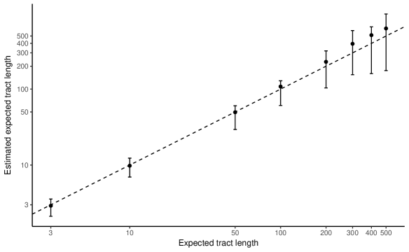
Figure 1: Expected IGC tract length versus estimates with maximum composite likelihood from simulated data. All simulation scenarios used a value of $\tau=\eta/p=5.16$. One hundred data sets were simulated for each true value of $1/p$. As described in the text, maximum composite likelihood estimates of $1/p$ that exceeded the true value by a factor of $10$ or more were excluded for the sample mean calculation but were included for the reported interquartile range values. The x-axis shows the true value of the expected IGC tract length (i.e., $1/p$) and the y-axis shows sample means among estimates with vertical line segments depicting interquartile ranges of the estimates. The dashed line shows $Y=X$.

3.2 Analyses of Actual Data

We applied the PS approach to analyze three groups of datasets. The first group consists of the $14$ data sets that Ji et al. (2016) analyzed with their codon-based IS approach for studying IGC. The second group is actually a single primate data set that Zhang et al. (1998) considered in their pioneering work on the origin of gene function. The third group of data sets are segmentally-duplicated intron regions from primates. Harpak et al. (2017) studied the effects of IGC on these intron regions with their binary-state treatment and we chose these data to examine how IGC inferences are affected by instead using maximum composite likelihood with a nucleotide-based model.

3.2.1 Yeast Paralogs

Yeast experienced an ancient genome-wide duplication (Wolfe and Shields 1997; Philippsen et al. 1997; Kellis et al. 2004; Dietrich et al. 2004; Dujon et al. 2004). Ji et al. (2016) analyzed 14 data sets of yeast protein-coding genes to characterize IGC that occurred subsequent to the genome-wide duplication. These data sets were the only ones that remained after applying stringent filters that were designed to reduce concerns about sequence alignment and paralogy status (see Ji et al. 2016). While the filters did not require it, all 14 data sets happen to encode ribosomal proteins. In every data set, six yeast species are each represented by two paralogs that stem from the ancient genome-wide duplication. Each data set also includes a sequence from a species (L. kluyveri) that diverged from the other six prior to the genome-wide duplication. The species represented in these data sets are related by the well-established phylogenetic tree topology of Figure 2.

Table LABEL:tab:IS-IGCYeastResults summarizes some of the results obtained by analyzing the 14 yeast data sets with the HKY+IS-IGC model. As was the case when these data sets were analyzed with the codon-based model of Ji et al. (2016), Table LABEL:tab:IS-IGCYeastResults shows that a substantial proportion of sequence change is attributed to IGC by both the HKY+IS-IGC and HKY+PS-IGC models. Table LABEL:tab:IGCestimates contrasts other inferences from the HKY+IS-IGC and HKY+PS-IGC models for these 14 data sets. It shows both models yield very similar estimates of $\tau$. Also, Table LABEL:tab:IGCestimates reveals that the expected fixed IGC tract lengths tend to be quite short according to the HKY+PS-IGC estimates. In fact, only 1 of the 14 data sets yields an expected tract length that exceeds 100 nucleotides and 8 of the 14 data sets yield expected tract lengths that are less than 20 nucleotides.

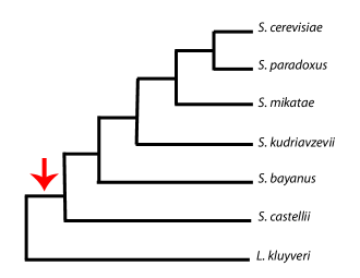
Figure 2: The tree topology used for evolutionary analyses of the yeast datasets. The arrow indicates the branch on which the genome-wide duplication occurred.

3.2.2 Primate EDN and ECP

Zhang et al. (1998) studied primate paralogs that encode eosinophil cationic protein (ECP) and eosinophil-derived neurotoxin (EDN). As described in the Materials and Methods, we used the sequence data and tree topology (see Figure 3) of Zhang et al. (1998).

We analyzed these data with both the IS and PS frameworks. Whereas our PS implementation has the advantage of accounting for IGC tracts, our IS implementation is computationally feasible with codon-based substitution models. Using an adaptation of the Muse-Gaut codon model (Muse and Gaut, 1994) that we will denote the MG94+IS-IGC model (see Ji et al. 2016) and considering the changes that occurred subsequent to the EDN/ECP duplication, we estimate that approximately 10.3% of the codon substitutions originated with an IGC event rather than a point mutation.

In Ji et al. (2016), we introduced a “paralog-swapping” procedure that is intended to investigate whether inferred IGC levels are not actually due to IGC events but are instead attributable to estimation artifacts that arise because of imperfect evolutionary models. The paralog-swapping procedure uses the two paralogs from each of two taxa that are descended from a post-duplication speciation event. It compares the biologically plausible scenario where IGC involves paralogs in the same genome to a biologically implausible scenario that has IGC between paralogs in different genomes (see Figure 4). The idea underlying the paralog-swapping procedure is that the inferred IGC levels will be similar between the two scenarios if artifacts due to unrealistic evolutionary models are generating the putative IGC signal. When we apply the paralog-swapping procedure in conjunction with the HKY+IS-IGC model, we infer much more IGC with the biologically plausible scenario. With the biologically plausible scenario of Figure 4A, the IGC parameter $\tau$ is estimated to be about $0.28$. With the biologically implausible scenario of Figure 4B, the IGC parameter $\tau$ is estimated to be about $0.00004$ (i.e., very close to $0$).

Table LABEL:tab:IS-IGCYeastResults includes results obtained by analyzing the EDN/ECP data set with the HKY+IS-IGC model. While the proportion of sequence change attributable to IGC is smaller for the EDN/ECP data set than any of the 14 yeast data sets, Table LABEL:tab:IS-IGCYeastResults shows that this inferred proportion is substantial whether the EDN/ECP data are analyzed with the HKY+IS-IGC model or the codon-based IGC treatment of Ji et al. (2016). As was the case for most of the yeast data sets, Table LABEL:tab:IGCestimates shows that the fixed IGC tract lengths that are inferred from EDN/ECP are very short.

Figure 3: The tree topology used for evolutionary analysis of primate EDN and ECP genes. The arrow indicates the duplication event.

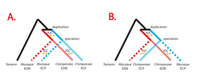
Figure 4: A paralog-swapping experiment addressing whether improvement to model fit can be attributed to IGC or to artifacts. Both Scenarios $A$ and $B$ specify the correct phylogeny between Tamarin and the paralogs of Macaque and Chimpanzee. Scenario $A$ shows the biologically correct situation that has the IGC between paralogs in the same genome. In Scenario $B$, IGC homogenization events involve one paralog in Macaque and one from Chimpanzee. Because Scenario $A$ corresponds to how observed data are generated, Scenario $A$ should fit better than Scenario $B$ if IGC is actually being detected. Note that this paralog-swapping experiment would not be possible if only $1$ postduplication species was used and would not be effective with more than two postduplication species.

3.2.3 Primate Introns

Harpak et al. (2017) examined the effects of IGC on the evolution of segmentally-duplicated primate introns. Here, we analyze a subset of the same data set in order to characterize IGC with our more parameter-rich models. As described in the Materials and Methods, we further filtered the introns of Harpak et al. (2017) to yield 20 data subsets where all ingroup species have two paralogs and the outgroup species has one paralog. This was done to lessen uncertainty regarding paralogy versus orthology. This filter also serves to make a single branch on the rooted primate tree be where the duplication event likely occurred for all 20 data subsets.

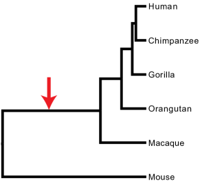
Figure 5: The tree topology used for evolutionary analysis of the primate intronic sequences. The arrow indicates the segmental duplication event.

Table LABEL:tab:IS-IGCYeastResults includes results obtained by analyzing the primate introns under the HKY+IS-IGC model that has no rate heterogeneity (i.e. $r_{2}=r_{3}=1$). It shows that the proportion of sequence change attributable to IGC is smaller for the primate intron data than for EDN/ECP and than for each of the 14 yeast data sets, but this proportion is still relatively large. In contrast to the results from the yeast and EDN/ECP protein-coding data, Table LABEL:tab:IGCestimates shows that the fixed IGC tract lengths that are estimated from the intron data have expected values that exceed several hundred nucleotides.

4 Discussion

4.1 Fixed IGC tracts inferred to be short

A distinction can be made between the lengths of IGC mutations and the lengths of IGC tracts that experience fixation. Measurements of the lengths of IGC mutations vary widely among studies and model systems, with some events affecting only about $10$ nucleotides and with more typical lengths involving hundreds of consecutive positions (e.g., see Chen et al. 2007; Mansai et al. 2011). Our estimates of the mean lengths of fixed IGC tracts also exhibit substantial variation (see Table LABEL:tab:IGCestimates). Whereas our estimates of the mean fixed IGC tract lengths from intron data tend to be not dramatically different than tract length estimates for IGC mutations, our estimates from exon data of the lengths of fixed IGC tracts (see Table LABEL:tab:IGCestimates) are substantially smaller than are usually obtained from studies of IGC mutations. This disparity may be partially attributable to homologous recombination events that occur subsequent to IGC mutation and that could thereby make the lengths of fixed IGC tracts shorter than the length of the original IGC mutations.

Natural selection may enhance the disparity between lengths of IGC mutation tracts and lengths of fixed tracts. IGC mutations can simultaneously introduce multiple fitness-affecting sequence changes into a paralog. Some of the changes may be advantageous whereas others may be deleterious. Subsequent homologous recombination may separate the advantageous and disadvantageous changes and thereby favor the fixation of IGC tracts that are shorter than the lengths of the original IGC mutations.

Biologically implausible evolutionary models represent a more mundane explanation for the short lengths that we estimate for fixed exonic IGC tracts. One shortcoming of the analyses presented here is that our treatment of changes due to IGC is more unrealistic than the treatment of substitutions that originated with point mutation. For nucleotide substitutions that originated by point mutation, the pair-site approach reflects the difference of fixation rates among the three codon positions by setting the relative rate at the first codon position to $1$ and adding a separate relative rate parameter for the second position (e.g., $r_{2}$) and another for the third position (e.g., $r_{3}$). However, the pair-site approach does not have differential fixation rates according to which codon positions are affected by the IGC event. This IGC treatment is convenient for setting up the statistical model but may be biologically unrealistic. Furthermore, we assume that IGC mutations occur and fix at a rate that is independent of the differences between the IGC donor and recipient tracts. This assumption violates evidence that IGC mutations become less likely as paralogs diverge (see Chen et al. 2007).

Whereas the exons analyzed in this study are from genes that contain either no intron or a short one, further investigations with more genes and more sophisticated IGC models may shed light on whether fixed IGC stretches really are shorter in exons than introns. These future investigations might benefit from studying protein-coding genes with both long coding regions and long introns.

4.2 IGC inference procedures

Harpak et al. (2017) recently developed two inferential procedures so that they could study IGC in segmentally-duplicated regions of humans and other primates. One of these procedures employed a hidden Markov model (HMM) that relied on the assumption that each sequence site has experienced either $0$ or $1$ IGC events subsequent to the duplication that created the paralogs being studied. Based on analyses of simulated data, we found a closely related but distinct HMM procedure to yield misleading estimates of expected IGC tract lengths, possibly because the IGC levels that were examined caused serious violations of the HMM assumptions (Ji, 2017). HMM approaches have proven useful for diverse DNA and protein sequence analysis tasks, but their value for studying IGC is likely to be particularly sensitive to how closely aligned are the HMM assumptions to the data being analyzed.

The other inferential procedure explored by Harpak et al. (2017) was a pair-site IGC treatment that resembles the one introduced here (see also Ji 2017). An attractive feature of the pair-site approaches is that they employ maximum composite likelihood for inference rather than relying on HMM assumptions that are most justified when IGC is rare. The pair-site approach of Harpak et al. (2017) considers two sites and two paralogs jointly but treats all sequence sites as being binary in nature. As a result, their joint state space has a size of $2^{4}=16$ where each site has two possible states representing two allele types with one state being the nucleotide type observed in mouse and with the other binary state collectively representing the other $3$ nucleotide types. Furthermore, Harpak et al. assume constant generation time and known divergence times on the lineage separating the primates from their most recent common ancestor with mouse. The Harpak et al. pair-site approach seems most appropriate for evolutionary scales where sequence changes are rare and where species are relatively closely related so that parameters such as generation time have little variation across the tree. It may be less satisfactory for larger timescales, such as the one that encompasses the period from the common ancestor of rodents and primates to the current day. In contrast, our parameterizations have been aimed at timescales of this magnitude.

Harpak et al. concluded from their intron analyses that the IGC rate per sequence position is an order of magnitude faster than the point mutation rate. Because the rates of the IS-IGC and PS-IGC approaches are normalized so that the expected rate per paralog per site is $1$ for substitutions that originated with a point mutation, our estimated $\tau$ values of approximately $0.5$ from both the IS-IGC and the PS-IGC approaches suggest that IGC happens at roughly the same rate per site of each paralog as point mutation. In addition, we estimate the percentage of nucleotide substitutions that originate with an IGC event rather than a point mutation to be $9.3\%$ for the filtered intron datasets. The estimated average tract length from our PS-IGC approach has the same order of magnitude as estimated by Harpak et al.. Because of the substantial differences between our analyses and those of Harpak et al., it is unclear how to isolate the cause of the different results.

4.3 Abundant substitution due to IGC

Following Ji et al. (2016), we used the MG94+IS-IGC model to estimate the proportion of fixed codon changes that were attributable to IGC rather than point mutation. We also employed the HKY+IS-IGC model to infer the proportion of nucleotide changes that were attributable to IGC rather than point mutation. For both the Yeast data sets and the primate EDN/ECP data, the estimated proportions are somewhat higher for the HKY+IS-IGC model than for the MG94+IS-IGC model (see Table LABEL:tab:IS-IGCYeastResults). While we expect the proportion for the HKY+IS-IGC model to be somewhat higher than for the MG94+IS-IGC model because individual events that change multiple codon positions are each only counted once in the MG94+IS-IGC calculations, we expect that most of the disparity in proportions is due to the differences between models.

While there is some disparity in IGC estimates among procedures, the more important message from Table LABEL:tab:IS-IGCYeastResults is there is a substantial amount of evolutionary change that is due to IGC. This has implications for the evolutionary consequences of gene duplications. Gene duplication is considered an important source of novel gene function. After their formation, duplicated genes may experience neo-functionalization, sub-functionalization or become pseudogenized (e.g., see Lynch and Conery 2000; Walsh 2003). In the absence of IGC, these events are determined by mutations accumulating independently at each paralog. Teshima and Innan (2008) showed that IGC can slow down the fixation of the neofunctionalized paralog by overwriting the neofunctionalized paralog sequence by that of another paralog. In this way, IGC can oppose natural selection. Furthermore, consideration of IGC could potentially improve the dating of subfunctionalization or neofunctionalization events.

Our conclusion is that fixation of IGC mutations is an important source of evolutionary change in multigene families. While the relative rate of IGC experienced per site (i.e., $\tau$) can be relatively well estimated by our IS and PS techniques, our PS approach yielded estimates of mean tract length from protein-coding data that were unexpectedly short and that were associated with high degrees of uncertainty. This motivates development of additional inference procedures that might be better than the PS procedure at extracting IGC tract information. In addition, there is ample room for improvement of IGC inference procedures. One important future direction will be to have the inference procedures assess how IGC rates decrease with paralog divergence. In addition, many multigene families consist of more than two paralogs and methods are needed for characterizing IGC in these cases. Because our analyses suggest that IGC is responsible for a substantial proportion of molecular evolution in multigene families, we believe that improved IGC inference should be a high priority.

5 Materials and Methods

5.1 Rate Normalization

For all analyses, substitution rates were normalized so that the expected rate per paralog per nucleotide is $1$ for substitutions that originated with a point mutation and so that the reported values of $\tau$ can then be compared to this normalized value. The normalization leads to one unit of branch length representing one expected substitution arising from point mutation per paralog per site. Because the model has rate heterogeneity among the three codon positions, the normalization to an average rate of $1$ yields respective expected rates of $3/(1+r_{2}+r_{3})$, $3r_{2}/(1+r_{2}+r_{3})$, and $3r_{3}/(1+r_{2}+r_{3})$ at the first, second, and third codon positions.

5.2 Simulations

The Materials and Methods of Ji et al. (2016) describe how and why data sets were simulated using parameter values estimated from the YDR418W_YEL054C data set. With the same simulation procedure and for the same reasons, we again based our simulations on the YDR418W_YEL054C data set. However, this time we used the inferred values of the HKY+IS-IGC parameters from the YDR418W_YEL054C data to simulate data sets.

The estimated value of $\tau=\eta/p$ was $5.16$ for the YDR418W_YEL054C data set. We wanted to explore how the composite likelihood estimates of expected tract length $1/p$ varied for different true values of $1/p$. Because $\eta=\tau/(1/p)$, we used $\tau=5.16$ and each value of $1/p$ that was explored in the simulations to set the corresponding value of $\eta$. All other parameters were set at the values inferred by maximum composite likelihood from the YDR418W_YEL054C data set.

To match the YDR418W_YEL054C data, IGC and point mutation events were simulated according to the yeast species tree for sequences of length 492 nucleotides. While the simulations in Ji et al. (2016) operated at the codon level, these simulations used nucleotides as the units because the modified HKY model is a nucleotide substitution model that has independent evolution at the three codon positions but has different rates for each codon position. The nucleotides in three alignment columns (i.e., columns 238, 239, 240) were removed from each simulated data set because the actual YDR418W_YER054C data has a gap in these columns. For each simulation condition, 100 data sets were generated.

For each simulation scenario, one hundred data sets were simulated and analyzed with the HKY+PS-IGC model. Rather than finding the combination of parameter values that jointly maximize the composite likelihood, computational concerns and numerical optimization difficulties resulted in our instead optimizing the composite likelihood only over the tract length parameter $p$ with all other free parameters constrained at the values that were used to simulate the data sets. We note that the parameter $\tau=\eta/p$. By constraining $\tau$ at its true value and then inferring $p$, a value for the IGC tract initiation parameter $\eta$ is simultaneously inferred (i.e., $\eta=\frac{\tau}{(1/p)}$). While the computational shortcut of only inferring $p$ from simulated data is not ideal, the simulation results of Ji et al. (2016) indicated that the value of $\tau$ can be estimated relatively well.

5.3 Parametric Bootstrap Analyses

There were 100 replicates per parametric bootstrap analysis. The maximum composite likelihood procedure was employed to obtain estimates of model parameters from actual data and those estimated values were used to simulate data sets of the same size as the actual data. Each of the 100 simulated data sets was analyzed by the composite likelihood procedure and variability of the resulting estimates was summarized. Paralleling the analyses of simulated data sets described in Section 5.2, analyses of the 100 bootstrap replicates with the HKY+PS-IGC model were made computationally feasible by estimating the IGC tract length parameter $p$ but constraining all other free parameters to their true values. This imposition of constraints will presumably cause the uncertainty in the tract length parameter $p$ to be underestimated, but we hope that this underestimation is small given that $\tau=\eta/p$ and that Ji et al. (2016) found that the $\tau$ parameter of the IS model could usually be well estimated.

5.4 Yeast Data

In the Materials and Methods of Ji et al. (2016), we describe how the $14$ data sets of yeast protein-coding genes were selected and prepared. Although the 14 yeast data sets exclude introns, our pair-site analyses of these data attempted to accommodate the fact that an IGC tract may cross exon-intron boundaries. For each pair of S. cerevisiae paralogs that is listed in Table LABEL:tab:IS-IGCYeastResults and Table LABEL:tab:IGCestimates, we identified the exon-intron boundaries and intron lengths of the first of the listed S. cerevisiae paralogs. For each adjacent pair of columns in our alignment of yeast exons, we could therefore determine the separation along the gene sequence of the S. cerevisiae paralog that is listed first for each pair in Table LABEL:tab:IS-IGCYeastResults and Table LABEL:tab:IGCestimates. We then assumed that the gene sequence separation between adjacent exon columns for this S. cerevisiae paralog was identical to the gene sequence separation for all other paralogs in the exon alignment. Therefore, we did not attempt to account for insertions and deletions or for the possibility that exon-intron boundaries may vary along the evolutionary tree.

5.5 Primate EDN and ECP Data

We used the EDN and ECP sequence data from the Zhang et al. (1998) study and the tree topology that was first introduced by Rosenberg et al. (1995). Because of the relatively short time separating the common ancestor of humans and chimpanzees from the common ancestor of those two species with gorillas, we excluded human sequence data from our analyses to lessen the variation of gene tree and species tree topologies. The remaining species are gorilla (Gorilla gorilla), chimpanzee (Pan troglodytes), orangutan (Pongo pygmaeus), macaque (Macaca fascicularis), and tamarin (Saguinus oedipus). We obtained the protein-coding DNA sequences via their GenBank accession numbers and aligned them at the amino acid level with version 7.305b of the MAFFT software (Katoh and Standley, 2013). The protein sequence alignment was then converted to the corresponding codon-level alignment. Three codon columns that contain gaps were removed from the alignment. The remaining $157$ codon columns were used in the analyses.

5.6 Primate Intronic Data

We received $550$ sequence alignment files of the intronic data analyzed from Harpak et al. (2017). Each alignment file corresponds to one intron of a total of $75$ protein-coding gene pairs. We further filtered the alignment files to retain only those with both paralogs in the five ingroup species: human (Homo sapiens), chimpanzee (Pan troglodytes), gorilla (Gorilla gorilla), orangutan (Pongo abelii) and macaque (Macaca mulatta); and one paralog in the outgroup species: mouse (Mus musculus). This filter is intended to minimize uncertainties of gene duplication and loss histories so that the analyzed data is less likely to violate the gene tree topology that was assumed in our analyses. Twenty sets of paralogous introns and $15370$ sites remained after this filtering of alignment files. Each of these twenty sets of paralogous introns corresponds to one of five pairs of paralogs of protein-coding genes. The ensembl gene ids for the paralog pairs from human are: ENSG00000109272 and ENSG00000163737, ENSG00000136943 and ENSG00000135047, ENSG00000158485 and ENSG00000158477, ENSG00000163564 and ENSG00000163563, and
ENSG00000187626 and ENSG00000189298.

Because these sequence data represent introns rather than exons, we analyzed the 20 datasets with parameter values under the HKY+PS-IGC model that has no rate heterogeneity (i.e., $r_{2}=r_{3}=1$). In all analyses of the segmentally-duplicated intron data, we assumed that IGC tracts affecting one pair of intron paralogs in our data set would not also affect other pairs in our filtered data set. While this treatment of exon-intron boundaries is less sophisticated than that applied to the yeast and EDN/ECP data (see below), it is computationally less demanding than the treatment applied to those data.

We investigated two different sorts of analyses of the intron data. One sort consisted of grouping together all introns associated with the same gene. This results in the 20 intron subsets being divided into 5 groups. We separately analyzed each of the 5 groups. We constrained each intron assigned to a group to share parameter values with the other introns in the group. This treatment caused numerical optimization difficulties for most of the groups. Specifically, substantially different maximum composite likelihood estimates were obtained when numerical optimization was initiated from different sets of parameter values. We believe this difficulty arose because most of the 5 groups of introns contained little information about IGC tract lengths.

Due to this difficulty, we decided to share information across the 5 groups of introns by jointly analyzing them with the assumption that all introns shared the same parameter values. This corresponds to an assumption that the duplications that generated the 5 groups of introns all occurred at the same time. While this assumption neglects some variability in branch lengths among gene trees, it results in sharing information about IGC tract length distributions across the groups. Because this shared treatment resulted in less numerical optimization difficulty, all parameter estimates reported here for the intron data were obtained via the shared treatment.

5.7 Exon-Intron Boundaries

For yeast and primate EDN/ECP data, we only analyzed the coding sequences of protein-coding genes but we incorporated the possibility that individual IGC events could span entire introns and thereby affect consecutive exons. Consider two neighboring sites in the coding sequence that are at positions $k$ and $k+1$. Because of the possibility of introns, these two sites may not be neighbors in the gene sequence. We will assume these sites are separated in the gene sequence by $m$ nucleotides where $m\geq 1$ with $m=1$ being the case where the two sites are in the same exon. When the two sites are in different exons, our analyses have the distance $m$ between them be the length of the intron sequence plus one.

5.8 Numerical Optimization

Model parameters were estimated by numerically optimizing the logarithms of the composite likelihoods. Inferred parameters include branch lengths, parameters related to point mutation, and IGC-related parameters. The “L-BFGS-B” method from the scipy package (Oliphant, 2007; Walt et al., 2011) was employed for numerical optimization.

6 Acknowledgments

We thank Alexander Griffing, Hirohisa Kishino, Eric Stone, Ed Susko, and Marc Suchard for diverse assistance. We also thank Arbel Harpak for sharing his primate intron data. This work was supported by the National Institute of General Medical Sciences at the National Institutes of Health (GM118508) and the National Science Foundation (DEB 1754142). Data sets are available at https://github.com/xji3. Software for inferring IGC is available at https://github.com/xji3/IGCexpansion and http://jsonctmctree.readthedocs.org/en/latest/.

Table 1: HKY+IS-IGC results.

						HKY	MG94
Paralog Pair	LnL	Diff	$\tau$	$r_{2}$	$r_{3}$	Prop	Prop
YLR406C,YDL075W	-1189.81	26.55	5.10	0.43	8.08	0.24	0.20
YER131W,YGL189C	-1216.91	31.58	5.27	0.97	19.60	0.27	0.20
YML026C,YDR450W	-1368.47	94.72	12.85	0.27	9.67	0.40	0.34
YNL301C,YOL120C	-2126.64	129.75	7.94	0.57	7.16	0.32	0.26
YNL069C,YIL133C	-2332.61	74.95	3.63	0.43	4.78	0.26	0.22
YMR143W,YDL083C	-1217.38	52.80	9.19	0.13	17.72	0.31	0.29
YJL177W,YKL180W	-1840.38	63.64	6.45	0.50	8.97	0.28	0.21
YBR191W,YPL079W	-1468.95	91.84	13.66	0.15	6.39	0.40	0.32
YER074W,YIL069C	-1233.00	131.50	20.90	0.28	6.94	0.39	0.37
YDR418W,YEL054C	-1735.40	65.09	5.16	0.54	11.58	0.27	0.21
YBL087C,YER117W	-1372.91	79.96	11.05	0.34	10.59	0.38	0.29
YLR333C,YGR027C	-1246.67	108.84	9.88	0.60	8.05	0.39	0.29
YMR142C,YDL082W	-2033.88	179.32	14.37	1.12	8.42	0.42	0.38
YER102W,YBL072C	-2037.26	205.73	14.77	0.82	6.19	0.43	0.36
EDN/ECP	-1713.06	12.61	1.79	1.52	1.56	0.16	0.10
Introns	-62878.87	93.79	0.44	N.A.	N.A.	0.09	N.A.

• Each row begins with the name of the data set. Yeast datasets are named by the systematic names of the two S. cerevisiae paralogous open reading frames. The “EDN/ECP” row represents the primate EDN/ECP data set. The “Introns” row represents the segmentally-duplicated primate introns. The “lnL IS-IGC” column shows the maximum log-likelihood value of the HKY+IS-IGC model. The “Diff” column specifies the number of log-likelihood units by which the HKY+IS-IGC value exceeds the maximum log-likelihood value of same model when $\tau$ is constrained to $0$. The “$\tau$” column shows the estimated $\tau$ value from the HKY+IS-IGC model. The “$r_{2}$” and “$r_{3}$” columns show the estimated relative substitution rates of the second and third codon positions from the HKY+IS-IGC model. The column labelled “HKY Prop” shows the estimated proportions of nucleotide changes attributable to IGC with the HKY+IS-IGC model. The column labelled “MG94 Prop” shows the estimated proportions of codon changes attributable to IGC with the MG94+IS-IGC model. “N.A.” is written in table entries to denote “not applicable”.

Table 2: IGC parameter estimates.

	$\tau$ IS-IGC		$\tau$ PS-IGC	$1/p$ PS-IGC
Paralog Pair	MCLE	Interquartile	MCLE	MCLE	Interquartile
YLR406C,YDL075W	5.10	(4.37, 6.12)	5.10	4.04	(2.97, 4.87)
YER131W,YGL189C	5.27	(3.89, 6.75)	5.27	13.24	(9.46, 16.91)
YML026C,YDR450W	12.85	(10.46, 15.32)	12.84	1.04	(1.00, 1.27)
YNL301C,YOL120C	7.94	(6.88, 8.71)	7.93	103.52	(68.27, 141.12)
YNL069C,YIL133C	3.63	(3.15, 4.11)	3.63	12.37	(8.90, 13.20)
YMR143W,YDL083C	9.19	(7.28, 13.85)	9.20	4.79	(3.55, 6.45)
YJL177W,YKL180W	6.45	(5.13, 7.20)	6.45	8.50	(7.11, 10.53)
YBR191W,YPL079W	13.66	(10.99, 15.41)	13.65	9.08	(7.57, 10.78)
YER074W,YIL069C	20.90	(16.69, 24.06)	20.89	53.05	(38.86, 72.06)
YDR418W,YEL054C	5.16	(4.23, 6.48)	5.16	3.80	(3.13, 4.69)
YBL087C,YER117W	11.05	(8.76, 13.22)	11.03	29.45	(20.14, 38.67)
YLR333C,YGR027C	9.88	(8.11, 11.43)	9.85	36.68	(26.96, 53.72)
YMR142C,YDL082W	14.37	(11.80, 16.77)	14.36	33.61	(29.45, 46.62)
YER102W,YBL072C	14.77	(12.25, 16.36)	14.76	26.34	(20.61, 61.41)
EDN/ECP	1.79	(1.40, 2.21)	1.79	6.90	(4.32, 8.34)
Introns	0.44	(0.41, 0.46)	0.52	370.4	(142.9, 523.0)

• Each row begins with the name of the data set, as detailed in the caption to Table LABEL:tab:IS-IGCYeastResults. Columns labelled “MCLE” contain maximum composite likelihood estimates and columns labelled “Interquartile” represent the $25{\mbox{th}}$ and $75{\mbox{th}}$ percentiles of the estimated values in $100$ parametric bootstrap samples. The “$\tau$, IS-IGC” columns show the $\tau$ values estimated with the HKY+IS-IGC model. The “$\tau$, PS-IGC” column shows the $\tau$ values estimated with the HKY+PS-IGC model. Because the parametric bootstrap analyses for the HKY+PS-IGC model did not consider uncertainty in the $\tau$ parameter (see Materials and Methods), interquartile ranges are not available for these $\tau$ estimates. The “$1/p$, HKY+PS-IGC” columns show the average tract length in nucleotides of fixed IGC events as estimated with the HKY+PS-IGC model.

References

- Chen et al. (2007) Chen, J.-M., Cooper, D. N., Chuzhanova, N., Férec, C., and Patrinos, G. P. 2007. Gene conversion: mechanisms, evolution and human disease. Nature Reviews Genetics, 8(10): 762–775.
- Dietrich et al. (2004) Dietrich, F. S., Voegeli, S., Brachat, S., Lerch, A., Gates, K., Steiner, S., Mohr, C., Pöhlmann, R., Luedi, P., Choi, S., et al. 2004. The ashbya gossypii genome as a tool for mapping the ancient saccharomyces cerevisiae genome. Science, 304(5668): 304–307.
- Dujon et al. (2004) Dujon, B., Sherman, D., Fischer, G., Durrens, P., Casaregola, S., Lafontaine, I., De Montigny, J., Marck, C., Neuvéglise, C., Talla, E., et al. 2004. Genome evolution in yeasts. Nature, 430(6995): 35–44.
- Felsenstein (1981) Felsenstein, J. 1981. Evolutionary trees from dna sequences: a maximum likelihood approach. Journal of molecular evolution, 17(6): 368–376.
- Goldman (1993) Goldman, N. 1993. Statistical tests of models of dna substitution. Journal of Molecular Evolution, 36: 182–198.
- Harpak et al. (2017) Harpak, A., Lan, X., Gao, Z., and Pritchard, J. K. 2017. Frequent nonallelic gene conversion on the human lineage and its effect on the divergence of gene duplicates. Proceedings of the National Academy of Sciences, 114(48): 12779–12784.
- Hasegawa et al. (1985) Hasegawa, M., Kishino, H., and Yano, T.-a. 1985. Dating of the human-ape splitting by a molecular clock of mitochondrial dna. Journal of molecular evolution, 22(2): 160–174.
- Ji (2017) Ji, X. 2017. Phylogenetic approaches for quantifying interlocus gene conversion (doctoral dissertation). North Carolina State University Theses and Dissertations Database. http://www.lib.ncsu.edu/resolver/1840.20/34873.
- Ji et al. (2016) Ji, X., Griffing, A., and Thorne, J. L. 2016. A phylogenetic approach finds abundant interlocus gene conversion in yeast. Molecular biology and evolution, 33(9): 2469–2476.
- Katoh and Standley (2013) Katoh, K. and Standley, D. M. 2013. Mafft multiple sequence alignment software version 7: improvements in performance and usability. Molecular biology and evolution, 30(4): 772–780.
- Kellis et al. (2004) Kellis, M., Birren, B. W., and Lander, E. S. 2004. Proof and evolutionary analysis of ancient genome duplication in the yeast saccharomyces cerevisiae. Nature, 428(6983): 617–624.
- Kent (1982) Kent, J. T. 1982. Robust properties of likelihood ratio tests. Biometrika, 69(1): 19–27.
- Lynch and Conery (2000) Lynch, M. and Conery, J. S. 2000. The evolutionary fate and consequences of duplicate genes. Science, 290(5494): 1151–1155.
- Mansai et al. (2011) Mansai, S. P., Kado, T., and Innan, H. 2011. The rate and tract length of gene conversion between duplicated genes. Genes, 2(2): 313–331.
- McVean et al. (2002) McVean, G., Awadalla, P., and Fearnhead, P. 2002. A coalescent-based method for detecting and estimating recombination from gene sequences. Genetics, 160(3): 1231–1241.
- Muse and Gaut (1994) Muse, S. V. and Gaut, B. S. 1994. A likelihood approach for comparing synonymous and nonsynonymous nucleotide substitution rates, with application to the chloroplast genome. Molecular biology and evolution, 11(5): 715–724.
- Nasrallah et al. (2010) Nasrallah, C. A., Mathews, D. H., and Huelsenbeck, J. P. 2010. Quantifying the impact of dependent evolution among sites in phylogenetic inference. Systematic biology, 60(1): 60–73.
- Oliphant (2007) Oliphant, T. E. 2007. Python for scientific computing. Computing in Science & Engineering, 9(3).
- Philippsen et al. (1997) Philippsen, P., Kleine, K., Pöhlmann, R., Düsterhöft, A., Hamberg, K., Hegemann, J. H., Obermaier, B., Urrestarazu, L., Aert, R., Albermann, K., et al. 1997. The nucleotide sequence of saccharomyces cerevisiae chromosome xiv and its evolutionary implications. Nature, 387(6632 Suppl): 93–98.
- Robinson et al. (2003) Robinson, D. M., Jones, D. T., Kishino, H., Goldman, N., and Thorne, J. L. 2003. Protein evolution with dependence among codons due to tertiary structure. Molecular Biology and Evolution, 20(10): 1692–1704.
- Rosenberg et al. (1995) Rosenberg, H. F., Dyer, K. D., Tiffany, H. L., and Gonzalez, M. 1995. Rapid evolution of a unique family of primate ribonuclease genes. Nature genetics, 10(2): 219–223.
- Teshima and Innan (2008) Teshima, K. M. and Innan, H. 2008. Neofunctionalization of duplicated genes under the pressure of gene conversion. Genetics, 178(3): 1385–1398.
- Varin et al. (2011) Varin, C., Reid, N., and Firth, D. 2011. An overview of composite likelihood methods. Statistica Sinica, 21: 5–42.
- Walsh (2003) Walsh, B. 2003. Population-genetic models of the fates of duplicate genes. Genetica, 118(2-3): 279–294.
- Walt et al. (2011) Walt, S. v. d., Colbert, S. C., and Varoquaux, G. 2011. The numpy array: a structure for efficient numerical computation. Computing in Science & Engineering, 13(2): 22–30.
- Wolfe and Shields (1997) Wolfe, K. H. and Shields, D. C. 1997. Molecular evidence for an ancient duplication of the entire yeast genome. Nature, 387(6634): 708–713.
- Zhang et al. (1998) Zhang, J., Rosenberg, H. F., and Nei, M. 1998. Positive darwinian selection after gene duplication in primate ribonuclease genes. Proceedings of the National Academy of Sciences, 95(7): 3708–3713.