Online Causal Inference for Advertising in Real-Time Bidding Auctions

Abstract

Real-time bidding (RTB) systems, which utilize auctions to allocate user impressions to competing advertisers, continue to enjoy success in digital advertising. Assessing the effectiveness of such advertising remains a challenge in research and practice. This paper proposes a new approach to perform causal inference on advertising bought through such mechanisms. Leveraging the economic structure of first- and second-price auctions, we first show that the effects of advertising are identified by the optimal bids. Hence, since these optimal bids are the only objects that need to be recovered, we introduce an adapted Thompson sampling algorithm to solve a multi-armed bandit problem that succeeds in recovering such bids and, consequently, the effects of advertising while minimizing the costs of experimentation. We derive a regret bound for our algorithm which is order optimal and use data from RTB auctions to show that it outperforms commonly used methods that estimate the effects of advertising.

Keywords: Causal inference, multi-armed bandits, advertising auctions

1 Introduction

The dominant way of selling ad impressions on ad exchanges (AdXs) is through real-time bidding (RTB) systems. These systems utilize auctions to allocate user impressions arriving at digital publishers to competing advertisers or intermediaries such as demand side platforms (DSPs). Most RTB auctions on AdXs are single-unit second-price auctions (SPAs) or, more recently, single-unit first-price auctions (FPAs). The complexity and scale of available ad inventory, the speed of transactions, which allows little time for deliberation, and the complex nature of competition imply that advertisers participating in RTB auctions have significant uncertainty about the value of the impressions they are bidding for and the nature of the competition they face. Developing accurate and reliable ways of measuring the value of advertising in this environment is essential for advertisers to profitably trade on the exchange and to ensure that acquired ad impressions generate sufficient value. Measurement needs to deliver incremental effects of ads for different types of ad and impression characteristics and needs to be automated. Experimentation thus becomes attractive as a way to obtain credible estimates of such causal effects.

Motivated by this, the current paper presents a new approach to perform causal inference on RTB advertising in both SPA and FPA settings. Our approach enables learning heterogeneity in the inferred average causal effects across ad and impression characteristics. The novelty of the proposed approach is in addressing the two main challenges that confront developing a scalable experimental design for RTB advertising.

The first challenge is that measuring the average treatment effect ($ATE$) of advertising requires comparing outcomes of users who are exposed to ads with outcomes of users who are not. A complication of the RTB setting is that ad exposure is not under complete control of the experimenter because it is determined by an auction. This precludes simple experimental designs in which ad exposure is directly randomized. Instead, we need a design in which the experimenter controls only an input to the auction, bids, but wishes to perform inference on the effect of a stochastic outcome induced by this input, ad exposure.

The second challenge is the cost of experimentation on the AdX. Obtaining experimental impressions is costly: one has to win the auction to observe the outcome with ad exposure and lose the auction to observe the outcome without it. When bidding is not optimized, costs can be substantial. First, they can emerge from overbidding, in which case the realized cost is high because the paid bid is not compensated by the outcome that is obtained from winning the auction. Second, they can emerge from underbidding, in which case the opportunity cost from losing the auction is high because the outcome that is obtained from losing is lower than the outcome that would have been obtained from paying a high enough bid to win the auction. With potentially millions of auctions in an experiment, suboptimal bidding can make this experiment unviable. Therefore, to be successful an effective experimental design has to deliver inference on the causal effect of ads while also managing the cost of experimentation by implementing a bidding policy that is optimized to the value of the impressions encountered.

It is not obvious how to design an experiment that addresses both challenges simultaneously: optimal bidding requires knowing the value of each impression, which was the goal of experimentation in the first place. Therefore, online methods, which introduce randomization to induce exploration of the value of advertising and combine it with concurrent exploitation of the information learned to optimize bidding, become very attractive in such settings.

At the core of online methods is the need to balance the goal of learning the expected effect of ad exposure (henceforth called the advertiser’s “inference goal”) with the goal of learning the optimal bidding policy (henceforth called the advertiser’s “economic goal”). The tension is that finding the optimal bidding policy does not guarantee proper estimation of ad effects and vice versa. At one extreme, with a bidding policy that delivers on the economic goal, the advertiser could win most of the time, making it difficult to measure ad effects since outcomes with no ad exposures would be scarcely observed. At the other extreme, with pure bid randomization the advertiser could estimate ad effects and deliver on the inference goal, but may end up incurring large economic losses in the process.

Our contribution is to set the advertiser’s problem as a multi-armed bandit (MAB) problem and introduce a statistical learning framework that address both these considerations. In our design, observed heterogeneity is summarized by a context, $x$, bids form arms, and the advertiser’s monetary auction payoffs form the rewards, so that the best arm, or optimal bid, maximizes the advertiser’s expected payoff from auction participation given $x$. Exploiting the economic structure of SPAs and FPAs, we derive, under conditions we outline, the relationship between the optimal bid at a given $x$ and the $ATE$ of the ad at the value $x$, or $ATE(x)$. For SPAs, we show that these two objects are equal, so that, in our experimental design, the twin tasks of learning the optimal bidding policy and estimating ad effects not only can build off each other, but are perfectly aligned. For FPAs, we demonstrate that the two goals are closely related, though only imperfectly aligned. In either case, we show that the $ATE$s are identified from the optimal bids, so that properly addressing the economic goal, that is, solving the MAB problem, suffices to estimate ad effects in addition to learning the optimal bidding policy.

To implement our approach, we present a Thompson Sampling (TS) algorithm customized to our auction environment trained online via a Markov Chain Monte Carlo (MCMC) method. TS is a Bayesian approach, which is an attractive way of tackling this problem because it can easily incorporate prior information and flexibly exploits the shared information across arms and contexts. The algorithm adaptively chooses bids across rounds based on current estimates of which arm is the optimal one. These estimates are updated each round via MCMC through Gibbs sampling, which leverages data augmentation to impute the missing potential outcomes and the censored or missing competing bids. We demonstrate that our proposed method achieves a prior-free and order-optimal regret bound, which guarantees that it recovers the optimal arm asymptotically.

Using the iPinYou data set, which contains bidding from RTB auctions, we show that our proposed algorithm is able to recover the $ATE$s of advertising correctly and incurs in substantially lower costs of experimentation compared to non-adaptive “A/B/n” tests, explore-then-commit (ETC) strategies and a canonical off-the-shelf TS algorithm. This illustrates the viability of our proposed approach and demonstrates its superior performance against competing popular benchmarks on the twin goals of balancing inference and the costs of experimentation.

To summarize, the high level contributions of this paper are two-fold:

1. To our knowledge, this is the first paper that proposes a comprehensive solution to the vexing problem of measuring causal effects of advertising bought via RTB mechanisms on ad exchange, while directly tacking the problem of controlling the cost experimentation by optimizing the advertiser’s bidding in an internally consistent way. A simultaneous solution to doing causal measurement of ad-effects while keeping the experimental costs manageable in this way is critical given the scale and complexity of modern RTB exchanges, where ad-effects vary dramatically and are ex ante uncertain, and where bidding is a principal driver of ad spend and experimentation costs.

2. We show how the experimental design can be fused with economic theory (here of first- and second-price auctions) to make progress on improved ways of doing causal inference and experimentation. We believe this paper is the first to show the sense in which this fusion is valuable for auction-driven advertising and how it can be implemented in practice in RTB ads settings. While the current exposition is fine tuned to RTB, this fusion can be useful in other business contexts where the goal of experimentation is to drive precise business goals (so the payoffs from such experimentation, such as firms profits are well defined) and where economic theory and prior knowledge puts useful structure on the behavior of agents and systems. We elaborate further on this point in the conclusion section.

The rest of the paper discusses the relationship between the approach presented here with the existing literature and explains our contribution relative to existing work. The following section defines the design problem. Sections 3 and 4 show how we leverage auction theory to balance the experimenting advertiser’s objectives. Section 5 presents the modified TS algorithm we use to implement our approach. Section 6 displays results documenting the performance of the proposed algorithm and shows its advantages over competing designs. The last section concludes.

Related literature

Our paper lies at the intersection of three broad fields of study: online learning in ad auctions, experimentation in digital advertising, and causal inference with MABs. Given that each of these streams of literature is mature, for brevity we only discuss the papers to which ours is most closely related.

Online learning in ad auctions

Despite focusing primarily on causal inference, this paper closely relates to the literature on online learning in ad auctions since we solve an online learning-to-bid problem.

Many studies in this literature take the seller’s perspective and focus on designing mechanisms that maximize the seller’s expected profit (e.g., finding the optimal reserve price when the distribution of valuations of the bidders is unknown to the auctioneer). Examples include Cesa-Bianchi et al., (2014), Haoyu and Wei, (2020) and Kanoria and Nazerzadeh, (2021).

Our study relates more closely to studies that address the bidder’ learning-to-bid problem. In the context of FPAs, Balseiro et al., (2019), Han et al., 2020a and Han et al., 2020b present algorithms for contextual bandits that treat the bidder’s value for the ad as the context, implying that there is no need for causal inference because, as we show below, this value corresponds to the treatment effect of the ad. Weed et al., (2016) and Feng et al., (2018) relax the assumption that advertisers know their valuations before bidding and present learning-to-bid algorithms for SPAs. However, they also rule out the need for causal inference by assuming that the advertiser’s value for the ad can be observed when they win the auction and that the value is zero when they lose (as in canonical auction models). The latter assumption is also made in the causal model proposed by Bompaire et al., (2021). Yet, in the context of ads a user may have a non-zero propensity to buy the advertiser’s products even in the absence of ad exposure, and winning the auction changes this propensity, so this assumption may not be well suited. In contrast, this paper explicitly takes this into account to address the problem of bid optimization without ruling out the need for causal inference and adjusting the algorithm that recovers the optimal bid so that causal inference can be performed.

This paper is also related to recent studies that analyze market equilibrium when bidders learn their values by interacting in repeated RTB auctions. Examples include Dikkala and Tardos, (2013), who characterize an equilibrium credit provision strategy for an ad publisher who faces bidders in SPAs for ads, and Iyer et al., (2014), who adopt a mean-field approximation for large markets to study repeated SPAs and apply it to the problem of selecting optimal reserve prices for the publisher. Balseiro et al., (2015) characterize equilibrium strategic interactions between budget-constrained advertisers who face no uncertainty about their private valuations, but have uncertainty about the number, bids and budgets of their competitors. Finally, Balseiro and Gur, (2019) and Tunuguntla and Hoban, (2021) provide pacing algorithms under the same paradigm in repeated SPAs. Tunuguntla and Hoban, (2021) also discuss augmenting their algorithm with bandit exploration when the advertiser’s valuation has to be learned. Overall, the goals of these papers, to characterize equilibria and to suggest equilibrium budget pacing strategies, credits or reserve prices, are different from ours, which is to develop an approach to perform causal inference on the expected effect of ads bought via SPAs and FPAs.

A smaller literature uses more general reinforcement learning (RL) approaches to optimize RTB advertising policies (Cai et al.,, 2017; Wu et al.,, 2018; Jin et al.,, 2018). However, unlike us these papers are not concerned with performing causal inference. Because we tackle this goal by leveraging key properties of the auction format, we contribute to a nascent literature on direct applications of auction theory to enable causal inference. While several studies combined experimental designs with auction theory, their goals were to identify optimal policies such as bids as in the aforementioned studies, reserve prices (Austin et al.,, 2016; Ostrovsky and Schwarz,, 2016; Pouget-Abadie et al.,, 2018; Rhuggenaath et al.,, 2019), auction formats (Chawla et al.,, 2016) or more general mechanisms (Kandasamy et al.,, 2020), not to estimate the causal effect of an action such as advertising determined by the outcome of an auction, which is our goal.

Experimentation in digital advertising

This paper is related to the literature on experimental approaches to measure the effect of digital advertising. One feature that distinguishes this paper from several studies in this stream is its focus on developing an approach from the advertiser’s perspective as opposed to from the publisher’s perspective, such as “ghost-ads” for display advertising (Johnson et al.,, 2017) or search ads (Simonov et al.,, 2018), which require observation of auction logs or cooperation with the publisher for implementation. In RTB settings, the advertiser bidding on AdXs does not control the auction and does not have access to these logs, precluding the use of such approaches.

Existing approaches that take the advertiser’s perspective include geo-level randomization (Blake et al.,, 2015) or inducing randomization of ad intensities by manipulating ad campaign frequency caps on DSPs (Sahni et al.,, 2019). Unlike these papers, our method leverages bid randomization, is tailored to the RTB setting, is an online, rather than offline, inferential procedure, and leverages auction theory for inference.

Lewis and Wong, (2018) suggest using bid randomization to infer the causal effects of RTB ads. They use bids as an instrumental variable for ad exposures and recover the local average treatment effect, while we leverage auction theory to deliver $ATE$s for SPAs and FPAs. Also, unlike the experimental design outlined here, their method is not adaptive and involves pure exploration. Consequently, it does not attempt to minimize the costs of experimentation, which we do.

Adaptive experimental designs for picking the best creative for ad campaigns are presented in Scott, (2015), Schwartz et al., (2017), Ju et al., (2019) and Geng et al., (2020). The problem addressed in these papers of selecting a best performing variant from a set of candidates is conceptually distinct from the problem addressed in this paper of measuring the causal effect of an RTB ad campaign, and these papers also do not address bidding.

Finally, our approach also relates to that of Feit and Berman, (2019), who also advocate for experimental designs that are profit maximizing. Feit and Berman, (2019) use a two-period setup to study a treatment decision that is under the agent’s full control, while we adopt a many-period bandit-allocation and show how to implement profit maximizing experiments for outcomes over which the advertiser only has imperfect control.

Causal inference with multi-armed bandits

Existing approaches to causal inference with MABs differ based on whether they pertain to offline settings, where pre-collected data are available to the analyst, or online settings, where data arrive sequentially, with latter being relatively more recent. This paper relates more closely to the online stream, so we discuss only papers related to online inference.

Performing causal inference with MABs is complicated by the adaptive nature of data collection, wherein future data collection depends on the data already collected. Although several algorithms that MAB problems possess attractive properties for finding the best arm, estimates of arm-specific expected rewards typically exhibit “adaptive bias” (Xu et al.,, 2013; Villar et al.,, 2015). Nie et al., (2018) showed that archetypal algorithms such as Upper Confidence Bound (UCB) and TS compute estimates of arm-specific expected rewards that are biased downwards. Hence, leveraging MABs for causal inference for RTB ads is hindered even if ad exposures are under complete control of the advertiser. If we set up ad exposure and no ad exposure as arms, so that the difference in rewards between the two arms represents the causal effect of the ad, and use a typical algorithm to solve the MAB, adaptive bias in estimating the respective arm-specific expected rewards will not yield the true expected effect of ad exposures.

Online methods to find the best arm while correcting for such adaptive bias include Goldenshluger and Zeevi, (2013), Nie et al., (2018), and Bastani and Bayati, (2020), who suggest data-splitting by forced sampling of arms at prescribed times, and Dimakopoulou et al., (2018) and Hadad et al., (2021), who correct for the bias via balancing and inverse probability weighting. These studies aim to estimate without bias the expected reward associated with the best arm. In contrast, our goal is to obtain an unbiased estimate of the effect of an action (ad exposure) that is imperfectly obtained by pulling arms (i.e., placing bids), so that our target treatment whose effect is to be learned is not an arm, but a shared stochastic outcome that arises from pulling arms. Hence, arms are more appropriately thought of as encouragements for treatments, which is analogous to an offline encouragement design (e.g., Imbens and Rubin,, 1997). In addition, our approach presents a different way of avoiding adaptive bias because the object we seek to estimate and perform inference on relies on the identity of the best arm rather than the expected value of its reward. When a MAB algorithm can correctly recover the identity of the best arm, we can then leverage it for inference on ad effects in an online environment. This is achieved by maintaining a close link to auction theory, which makes our approach different in spirit from the above, more theory-agnostic approaches.

Our setup also shares similarities with the instrument-armed bandit setup of Kallus, (2018), in which there is a difference between the treatment-arm pulled and the treatment-arm applied due to the possibility of unit non-compliance. However, the difference between the pulled and applied treatments, which is important to the design here, is not a feature of the design considered by Kallus, (2018), because the pulled and applied treatments belong to the same set in his design. Also, unlike the setup in Kallus, (2018), where exposure to a treatment is the outcome of a choice by the unit to comply, exposure here is determined by a game that is not directly affected by the unit, which characterizes a different exposure mechanism.

MABs have been explicitly embedded within the structural causal framework of Pearl, (2009) in Bareinboim et al., (2015), Lattimore et al., (2016) and Forney et al., (2017). Our paper relates to them as our setting is a specific instance of a structural causal model tailored to the auction setting: we assume the existence of a probabilistic generative process that is the shared causal structure behind the distributions of the rewards of each arm. As this stream has emphasized, the link to the model in our application is helpful to making progress on the inference problem.

2 Problem formulation

Our goal is to develop a method to measure the effect of exposing users to ads an advertiser buys programmatically on AdXs. To buy an impression opportunity, advertisers need to participate in an auction ran by the AdX for each impression opportunity. Winning the auction allows advertisers to display their ads to users. In what follows, we will take the perspective of a focal advertiser that experiments to recover the expected effect of exposing users to their ad.

We define an advertiser’s goal of estimating the expected effect of displaying their ad to a user as the inference goal. To state this goal more precisely, let $Y(1)$ denote the revenue the advertiser receives when their ad is shown to the user and let $Y(0)$ denote the revenue they receive when their ad is not shown. The potential outcomes $Y(1)$ and $Y(0)$ are are expressed in monetary units and the effect of displaying the ad is $Y(1)-Y(0)$. All the information the advertiser has about the user and impression opportunity is captured by a variable $x\in\mathbb{X}$.

Therefore, the advertiser’s inference goal is to estimate a set of conditional average treatment effects, in which exposure to the ad is the treatment. They are given by $ATE(x)=\mathbb{E}\left[Y(1)-Y(0)\middle|x\right]$. The advertiser needs to estimate this object because they do not have complete knowledge of the distribution of potential outcomes $Y(1)$ and $Y(0)$ given $x$. Thus, achieving the inference goal requires the collection of data informative of this distribution.

A method that accomplishes the inference goal has to address four issues, which we discuss below. All four are generated by the distinguishing feature of the AdX environment that the treatment, exposure to the ad, can only be obtained by winning an auction.

Issue 1: The advertiser cannot randomize treatment directly

The first issue is that because treatment is determined by an auction over which the advertiser has no complete control, methods that rely on treatment randomization are not available. The outcome of the auction is not under the advertiser’s complete control because they do not determine the bids they compete against.

Although exposure to the ad cannot be perfectly controlled, participation in auctions is under the advertiser’s control. Therefore, a viable alternative design involves randomizing their participation across auctions. Without loss of generality, we can think of auction participation randomization as analogous to bid randomization, with “no participation” corresponding to a bid of $0$ and “participation” corresponding to a positive bid. However, as we discuss below, bid randomization does not suffice to identify causal effects without additional assumptions.

Issue 2: Bid randomization alone is insufficient for identification

The second issue is that the auction environment constrains what can be learned from designs that rely on bid randomization. In general, bid randomization is not sufficient to identify $ATE$s if the relationship between $Y(1)$, $Y(0)$ and competing bids remains unrestricted.

To see this, denote the highest bid against which the advertiser competes by $B_{CP}$. For simplicity, assume that $x$ can only take one value and hence can be ignored. Let $D\equiv\mathbbm{1}\left\{B_{CP}\leq b\right\}$ denote winning the auction, where $b$ is the advertiser’s bid. The observed outcome, $Y$, is given by $Y=D\times Y(1)+(1-D)\times Y(0)$. Further let $Y(1)=\lambda_{1}+\eta_{1}$ and $Y(0)=\lambda_{0}+\eta_{0}$, where $\lambda_{1}$ and $\lambda_{0}$ are constants, and $\eta_{1}$ and $\eta_{0}$ are error terms such that $\mathbb{E}[\eta_{1}]=\mathbb{E}[\eta_{0}]=0$. Hence, $ATE=\lambda_{1}-\lambda_{0}$.

Consider estimating the $ATE$ via a simple linear regression. A regression of $Y$ on $D$ using data collected with bid randomization corresponds to:

$$Y_{i} =\lambda_{0}+ATE\times D_{i}+D_{i}\eta_{1i}+(1-D_{i})\eta_{0i},$$ (1)

where $i$ indexes an observation. For the OLS estimator of $ATE$ to be consistent, the indicator $D_{i}$ has to be uncorrelated with $\eta_{1i}$ and $\eta_{0i}$. There are two potential sources of such correlation, $b$ and $B_{CP}$. Even if $b$ is picked at random, a correlation can still exist through $B_{CP}$. This motivates Assumption 1 below, which we maintain for the rest of the paper.

Assumption 1.

Conditional independence (“private values”) For all $x\in\mathbb{X}$, $\left\{Y(1),Y(0)\right\}\mathchoice{\mathrel{\hbox to0.0pt{$\displaystyle\perp$\hss}\mkern 2.0mu{\displaystyle\perp}}}{\mathrel{\hbox to0.0pt{$\textstyle\perp$\hss}\mkern 2.0mu{\textstyle\perp}}}{\mathrel{\hbox to0.0pt{$\scriptstyle\perp$\hss}\mkern 2.0mu{\scriptstyle\perp}}}{\mathrel{\hbox to0.0pt{$\scriptscriptstyle\perp$\hss}\mkern 2.0mu{\scriptscriptstyle\perp}}}B_{CP}|x$.

One way to interpret Assumption 1 is from an auction-theoretic perspective. It implies that, conditional on $x$, knowledge of $B_{CP}$ has no effect on the advertiser’s assessment of $Y(1)$ and $Y(0)$. Since these potential outcomes are the determinants of the advertiser’s willingness-to-pay, or valuation, to expose users to their ad, we can think of Assumption 1 as analogous to a private values condition. This does not mean that there cannot be correlations between the values that competing advertisers assign to an impression. The maintained assumption is that these common components of bidder valuations are captured by $x$. Part of the motivation arises from the programmatic bidding environment. When advertisers bid in AdXs, they match the ID (cookie/mobile-identifier) of the impression with their own private data. If $x$ captures a lot of information and encompasses what can be commonly known about the impression, advertisers’ valuations after conditioning on $x$ would only be weakly correlated or not at all.

An alternative way of interpreting Assumption 1 is in causal inference terms as an unconfoundedness assumption. Statistically, it is a conditional independence assumption, which is more likely to hold when $x$ captures a lot of information and encompasses what can be commonly known about the impression. This is most likely to happen when the experimenter is a large advertiser or an intermediary such as a large DSP, which has access to large amounts of user data that can be matched to auctioned impressions in real-time.

Along with bid randomization, Assumption 1 yields identification of $ATE$. From equation (1), OLS can estimate $ATE$ consistently under this condition, because both $b$ and $B_{CP}$ become independent of $\eta_{1}$ and $\eta_{0}$.

Issue 3: High costs of experimentation

While bid randomization combined with Assumption 1 is sufficient for identification of $ATE$s, a third issue to consider is the cost of experimentation. Exposure to an ad requires paying the winning price of an auction, while no exposure involves foregoing the value that would have been generated from displaying the ad. Therefore, collecting experimental units on the AdX involves both realized and opportunity costs.

These costs can be high under suboptimal bidding. Bidding higher than what is required to win an auction implies a waste of resources due to overbidding, and no bidding involves the opportunity costs from underbidding, especially from users to whom exposure to ads would have been beneficial. In a high frequency RTB environment, a typical experiment can involve millions of auctions, so that if bidding is not properly managed, the resulting economic losses can be substantial. These costs can form an impediment to implementing the experiment in practice.

The key to controlling costs is bid optimization, specifically by finding the optimal, expected payoff maximizing bid, $b^{*}(x)$, for each value of $x$. We refer to the advertiser’s goal of learning the optimal bidding policy in the experiment as their economic goal. As we discuss in detail below, the advertiser’s inference and economic goals are directly related, though not necessarily perfectly aligned.

To characterize the optimal bid and relate it to the advertiser’s inference goal, we first turn to the advertiser’s optimization problem from auction participation. The advertiser’s payoff as a function of their bid is denoted by $\pi\left[b,Y(1),Y(0),B_{CP}\right]$. We assume that the advertiser is risk neutral. In an SPA, $\pi(\cdot)$ is

$$\pi\left[b,Y(1),Y(0),B_{CP}\right] =\mathbbm{1}\left\{B_{CP}\leq b\right\}\times\left[Y(1)-B_{CP}\right]+\mathbbm{1}\left\{B_{CP}>b\right\}\times Y(0)$$

$$=\mathbbm{1}\left\{B_{CP}\leq b\right\}\times\left\{\left[Y(1)-Y(0)\right]-B_{CP}\right\}+Y(0),$$ (2)

while in an FPA $\pi(\cdot)$ is

$$\pi\left[b,Y(1),Y(0),B_{CP}\right] =\mathbbm{1}\left\{B_{CP}\leq b\right\}\times\left[Y(1)-b\right]+\mathbbm{1}\left\{B_{CP}>b\right\}\times Y(0)$$

$$=\mathbbm{1}\left\{B_{CP}\leq b\right\}\times\left\{\left[Y(1)-Y(0)\right]-b\right\}+Y(0).$$ (3)

Notice that the formulation of auction payoffs in equations (2) and (2) is different from typical auction setups. In most auction models, the term $Y(0)$ is set to zero because it is assumed that a bidder only accrues utility when they win the auction. However, this convention is not suitable to our setting given the interpretation of the terms $Y(1)$ and $Y(0)$. A consumer might have a baseline propensity to purchase the advertiser’s product even if they are not exposed to the ad, which is associated with the term $Y(0)$. Exposure to the ad might affect this propensity, implying that $Y(1)\neq Y(0)$.

The advertiser chooses a bid to maximize their expected payoff from auction participation, which is given by

$$\bar{\pi}(b|x)=\mathbb{E}\left\{\pi\left[b,Y(1),Y(0),B_{CP})\right]\middle|x\right\},$$ (4)

where the expectation is taken with respect to the distribution of $Y(1)$, $Y(0)$ and $B_{CP}$ on $x$. In addition to assuming that the advertiser does not fully know the distribution of $Y(1)$ and $Y(0)$, we further assume that they do not know the distribution of $B_{CP}$ as well. This implies that the advertiser faces uncertainty over the joint distribution of $Y(1)$, $Y(0)$ and $B_{CP}$ conditional on $x$, which we denote by $F\left(\cdot,\cdot,\cdot\middle|x\right)$. It is important to note that the fact that we postulate that there exists a distribution for $B_{CP}$ does not imply that competitors are randomizing bids or following mixed strategies, although it does allow for it. As in typical game-theoretic approaches to auctions, a given bidder, in this case the advertiser, treats the actions taken by their competitors as random variables, which is why we treat $B_{CP}$ as being drawn from a probability distribution.

Solving for $b^{*}(x)$ in the presence of uncertainty over $F\left(\cdot,\cdot,\cdot\middle|x\right)$ is neither standard nor trivial. It is not standard because, under the outlined circumstances, the advertiser faces two levels of uncertainty. The first, lower-order uncertainty is similar to the one faced by bidders in typical auction models: they are uncertain about what their competitors bid, which is encapsulated by $B_{CP}$. They are also uncertain about their own valuations, because, under this formulation, valuations correspond to the treatment effects, which are never observed in practice.

The second, higher-order uncertainty is not present in standard auction models and is the source of the inference goal. While in the majority of auction models a given bidder does not have complete knowledge of their valuation or of competing bids, they know the distributions from which these objects are drawn, which would correspond to the joint distribution of $Y(1)$, $Y(0)$ and $B_{CP}$ conditional on $x$. This is not the case here since the advertiser faces uncertainty regarding $F\left(\cdot,\cdot,\cdot\middle|x\right)$.

To see why this bidding problem is not trivial, notice that, without access to data informative of this distribution, the advertiser would have to integrate over $F\left(\cdot,\cdot,\cdot\middle|x\right)$ to construct the expected payoff from auction participation. The resulting optimization problem is:

$$\max_{b}\mathbb{E}_{F}\left(\mathbb{E}\left\{\pi\left[b,Y(1),Y(0),B_{CP}\right]\middle|F,x\right\}\middle|x\right).$$ (5)

In equation (5), the inner expectation is taken with respect to $Y(1)$, $Y(0)$ and $B_{CP}$ given their joint distribution given $x$, where $\pi\left[b,Y(1),Y(0),B_{CP}\right]$ is given in equations (2) and (2). Thus, it reflects the aforementioned lower-order uncertainty. In turn, the outer expectation is taken with respect to $F\left(\cdot,\cdot,\cdot\middle|x\right)$, which is reflected in the subscript “$F$” and on the conditioning on $F$ in the inner expectation. At the most general level, the advertiser would consider all trivariate probability distribution functions whose support was the three-dimensional positive real line. As such, the optimization problem given in (5) is not tractable, and the solution to this problem is in all likelihood highly sensitive to the beliefs over distributions the advertiser can have.

Without access to data, the advertiser would have no choice but to try to solve the optimization problem in (5). However, as we noted above, achieving the inference goal requires the collection of data, which can also be used to address the economic goal. Therefore, instead of tackling the optimization problem in (5), one strategy to optimize bidding would be to use the data collected in the experiment to construct updated estimates of $\mathbb{E}\left\{\pi\left[b,Y(1),Y(0),B_{CP}\right]\middle|F,x\right\}$, and optimize bids with respect to this estimate as the experiment progressed. This way, the data generated from the experiment would be used to address both the advertiser’s inference goal and to optimize expected profits to address their economic goal, so that both goals would be addressed simultaneously.

Issue 4: Aligning the inference and economic goals

The final issue is balancing the simultaneous pursuit of the inference and economic goals in the experiment. This issue arises because typical strategies aimed at tackling one of the goals can possibly have negative impacts on accomplishing the other, suggesting an apparent tension between the two.

To see this, consider what would happen if the experiment focused only on the advertiser’s inference goal by randomizing bids without any concurrent bid optimization. We already alluded to the consequences of this for the advertiser’s economic goal in our previous discussion: pure bid randomization can hurt the advertiser’s economic goal by inducing costs from suboptimal bidding. In particular, randomly submitted high bids can imply high realized costs due to winning impression opportunities at high prices, while randomly submitted low bids can lead to high opportunity costs due to missed beneficial impression opportunities.

Consider now what would happen if the experiment focused only on the advertiser’s economic goal. From equations (2), (2) and (4), the payoffs from bidding $b$ are stochastic from the advertiser’s perspective, and the optimal bid is the maximizer of the expected payoff from auction participation, $\bar{\pi}(b|x)$, which is unknown to the advertiser. Hence, pursuing the economic goal involves finding the best bid in an environment where payoffs are stochastic and maximizing expected payoffs against a distribution which has to be learned by exploration. An MAB or RL approach is thus attractive in this situation because it can recover $b^{*}(x)$ while minimizing the costs from suboptimal bidding, which pure randomization does not assess. By following this strategy, the advertiser would adaptively collect data to learn a good bidding policy by continuously re-estimating and re-optimizing $\bar{\pi}(b|x)$.

In principle, these data could also be used to estimate $ATE(x)$ by running the regression in (1) for each $x$, for example. However, the adaptive nature of the data collection procedure induces autocorrelation in the data, which can impact statistical properties of estimators. Moreover, even if all desired properties hold, underlying characteristics of the data and the algorithm used can affect the estimator adversely. To see this, consider the following example. For simplicity, assume once again that $x$ can be ignored and further assume that $\Pr(B_{CP}\leq b^{*})\approx 1$. A good algorithm would converge quickly, eventually yielding relatively few observations of $Y(0)$ compared to those of $Y(1)$, which would hinder the inference goal since typical estimators of $ATE$s based on such imbalanced data tend to be noisy.

This illustrates that the inference and economic goals can possibly be at odds despite being clearly related since they both depend on knowledge about the distribution $F\left(\cdot,\cdot,\cdot\middle|\cdot\right)$. The challenge faced by the advertiser to accomplish these goals is that this distribution is unknown, and while there are several approaches to gather data and tackle each goal in isolation, it is unclear whether they can perform satisfactorily in achieving both goals concurrently. We present a method to solve this issue next.

3 Balancing the advertiser’s objectives

We balance the two goals by leveraging the structure of the advertiser’s bid optimization problem, which shows how these goals are linked. Because bidding depends on the auction format, the extent to which the two goals are aligned differs across auction formats. We will show that in SPAs the inference and economic goals can be perfectly aligned, while in FPAs leveraging this linkage is still helpful, but the goals can only be imperfectly aligned.

To characterize our approach, we consider the limiting outcome of maximizing the true expected profit function with respect to bids when the joint distribution $F\left(\cdot,\cdot,\cdot\middle|\cdot\right)$ is known to the advertiser. In what follows, we will use the expressions in equations (2) and (2) ignoring the second term, $Y(0)$, because it does not depend on the advertiser’s bid. This expression also has the benefit of directly connecting the potential outcomes to this auction-theoretic setting, with the treatment effect $Y(1)-Y(0)$ taking the role of the advertiser’s valuation.

We combine equations (2) and (4) to write the object the advertiser aims to learn in an SPA as the maximizer with respect to $b$ of:

$$\bar{\pi}(b|x) \equiv\mathbb{E}\left\{\pi\left[b,Y(1),Y(0),B_{CP}\right]\middle|x\right\}$$

$$=\Pr\left(B_{CP}\leq b\middle|x\right)\times\mathbb{E}\left\{\left[Y(1)-Y(0)\right]-B_{CP}\middle|B_{CP}\leq b;x\right\}.$$ (6)

In an FPA, we combine equations (2) and (4) to write the object the advertiser aims to learn as the maximizer with respect to $b$ of:

$$\bar{\pi}(b|x) \equiv\mathbb{E}\left\{\pi\left[b,Y(1),Y(0),B_{CP}\right]\middle|x\right\}$$

$$=\Pr\left(B_{CP}\leq b\middle|x\right)\times\mathbb{E}\left\{\left[Y(1)-Y(0)\right]-b\middle|B_{CP}\leq b;x\right\}.$$ (7)

Once again, the expectations in equations (3) and (3) are taken with respect to $Y(1)$, $Y(0)$ and $B_{CP}$. The conditioning on the distribution $F$ is omitted since $\bar{\pi}\left(\cdot\middle|x\right)$ is the true expected profit function, which therefore utilizes the true conditional distribution $F\left(\cdot,\cdot,\cdot\middle|\cdot\right)$ to compute the relevant expectations and probabilities. We denote the maximizers of these respective expressions by $b^{*}(x)$. To ensure that $b^{*}(x)$ is well-defined, we maintain the following assumption on $F\left(\cdot,\cdot,\cdot\middle|\cdot\right)$.

Assumption 2.

Properties of $F\left(\cdot,\cdot,\cdot\middle|\cdot\right)$ For all $x\in\mathbb{X}$:
(i) The joint distribution $F(\cdot,\cdot,\cdot|x)$ admits a continuous density, $f(\cdot,\cdot,\cdot|x)$, over $\mathbb{R}_{+}^{3}$.
(ii) All variables are bounded: $Y(1)\leq\bar{y}_{1}<\infty$, $Y(0)\leq\bar{y}_{0}<\infty$, and $B_{CP}\leq\bar{b}_{CP}<\infty$.
(iii) The density of $B_{CP}$ given $x$, $f_{CP}\left(\cdot\middle|x\right)$, is strictly positive in the interior of $\mathbb{R}_{+}$.
(iv) The conditional reversed hazard rate of $B_{CP}$ given $x$, $\frac{f_{CP}\left(b_{CP}|x\right)}{F_{CP}\left(b_{CP}|x\right)}$, is decreasing in $b_{CP}$.

Assumption 2 outlines conditions on $F\left(\cdot,\cdot,\cdot\middle|\cdot\right)$ required for us to establish the results presented below. Not only are these conditions mild and relatively common in auction models, but they also can be relaxed as we discuss below. First, Assumption 2 is standard and made solely for tractability. It allows us not to have to address measurability technicalities throughout.

Assumption 2 is common in standard auction models but is actually stronger than what we require. To derive the optimal bids and establish that they are unique, we only need the expectations $\mathbb{E}\left[Y(1)|x\right]$, $\mathbb{E}\left[Y(0)|x\right]$ and $\mathbb{E}\left[B_{CP}|x\right]$ to be finite for every $x\in\mathbb{X}$, so that the expressions given in equations (3) and (3) are well-defined. This is the case if $Y(1)$, $Y(0)$ and $B_{CP}$ are bounded. The regret bound we present for the Thompson sampling algorithm proposed below requires the rewards given in equations (2) and (2) to follow a sub-Gaussian distribution. A sufficient condition for this to be the case is for rewards themselves to be bounded, which, in turn, is guaranteed by Assumption 2.

Assumption 2 is required for us to establish that the optimal bids are unique. As we discuss below, this is just a sufficient condition which can also be relaxed while maintaining uniqueness of optimal bids. Furthermore, notice that this condition is equivalent to an overlap assumption that $P(D=1|x)\in(0,1)$, where $P(D=1|x)$ is the propensity score. Because $D\equiv\mathbbm{1}\left\{B_{CP}\leq b\right\}$ and $P(D=1|x)\equiv P(B_{CP}\leq b|x)$, Assumption 2 implies that $P(B_{CP}\leq b|x)\in(0,1)$.

Finally, Assumption 2 is only required to determine $b^{*}(x)$ for FPAs. In particular, it is a sufficient condition for $b^{*}(x)$ to be unique. It states that the distribution of $B_{CP}$ conditional on $x$ has a decreasing reversed hazard rate. As argued by Block et al., (1998), this property holds for several distributions, including all decreasing hazard rate distributions and increasing hazard rate Weibull, gamma and lognormal distributions.

We now investigate the relationship between $b^{*}(\cdot)$ and $ATE(\cdot)$ under Assumptions 1 and 2. If the distribution $F\left(\cdot,\cdot,\cdot\middle|\cdot\right)$ was known, computing $ATE(\cdot)$ would be straightforward, as would be solving for $b^{*}(\cdot)$ by maximizing expression (3) or expression (3). The results below characterize this relationship first for SPAs and then for FPAs.

Proposition 1.

Optimal bid in SPAs Suppose that Assumptions 1, 2, 2 and 2 hold. If the auction is an SPA, then $b^{*}(x)=\max\left\{0,CATE(x)\right\}$.

The proof of Proposition 1 is given in Appendix A. It consists of demonstrating that Assumption 1 allows us to write the bidder’s expectation of their private valuation as $ATE(x)$. In turn, Assumptions 2, 2 and 2 give us the technical conditions to demonstrate that the optimal bid $b^{*}(x)$ is unique and equal to $\max\left\{0,ATE(x)\right\}$.

We now characterize the analogous relationship for FPAs.

Proposition 2.

Optimal bid in FPAs Suppose that Assumptions 1 and 2 hold. Let $\chi\left(b\middle|x\right)=b+\frac{F_{CP}\left(b|x\right)}{f_{CP}\left(b|x\right)}$. If the auction is an FPA, then $b^{*}(x)=\max\left\{0,\chi^{-1}\left[ATE(x)\middle|x\right]\right\}$.

The proof of Proposition 2 is given in Appendix A. The steps are the same as the proof for Proposition 1. The additional requirement that Assumption 2 holds is to demonstrate uniqueness of $b^{*}(x)$ and its equivalence to $\max\left\{0,\chi^{-1}\left[ATE(x)\middle|x\right]\right\}$. This additional requirement arises because for FPAs $b^{*}(x)$ is obtained from the first-order condition of the bidder’s optimization problem, whereas for SPAs we can obtain $b^{*}(x)$ simply by inspecting the bidder’s objective function.

The novelty of these results is that they are derived from an objective function that directly depends on the potential outcomes $Y(1)$ and $Y(0)$, which, as a result, constitute the advertiser’s willingness-to-pay for the auction impression. This creates a direct connection between the potential outcomes and the advertiser’s optimal bid, and while these connections resemble typical results from auction theory, they also have their particularities. The results above are necessary to derive these connections precisely.

Implications

Propositions 1 and 2 have three implications. First, they show how the optimal bids, $b^{*}(x)$, are related to $ATE(x)$. In an SPA, Proposition 1 shows that if displaying the ad is beneficial (i.e., $ATE(x)\geq 0$), the optimal bid is the $ATE(x)$ itself. In an FPA, Proposition 2 shows that whenever displaying the ad is beneficial, one should bid less than the $ATE(x)$ due to the typical bid shading that arises in FPAs. In turn, if displaying the ad is detrimental (i.e., $ATE(x)<0$), the advertiser would have no interest in displaying the ad in the first place, which can be guaranteed by a bid of zero. Consequently, the advertiser can follow a MAB or RL strategy in the experiment to learn $b^{*}(\cdot)$, and then obtain $ATE$s by leveraging these relationships. This will form the basis of the algorithm we propose in the next section.

Second, Propositions 1 and 2 show that, for both SPAs and FPAs, the object of inference, $ATE(x)$, is a common component of the expected payoff associated all bids one could consider for a given $x$. Thus, if one thinks of bids as arms, leveraging the economic structure of the problem induces cross-arm learning within each context (i.e., pulling each arm contributes to learning a common $ATE$).

Third, Propositions 1 and 2 show precisely how the inference and economic goals are connected. For SPAs, Proposition 1 is powerful because it implies that whenever displaying the ad is beneficial, the advertiser’s economic and inference goals are perfectly aligned, as learning $b^{*}(x)$ and estimating $ATE(x)$ consist of the same task. Our proposed experimental design for SPAs will be to find the best bid for each $x$, $b^{*}(x)$, and set that to be the $ATE(x)$.

In turn, our proposed experimental design for FPAs will be to find $b^{*}(x)$ for each $x$ and set $\chi\left[b^{*}(x)\middle|x\right]$ to be $ATE(x)$. However, because the inference and economic goals are not perfectly aligned, the estimator of $ATE(x)$ will also use an estimator of $F_{CP}(\cdot|x)$. Hence, unlike the estimator for SPAs, this estimator will have two sources of uncertainty around it: that of $b^{*}(x)$ and that of $F_{CP}(\cdot|x)$.

4 Accomplishing the advertiser’s objectives

We leverage Propositions 1 and 2 to develop a method that concurrently accomplishes the advertiser’s goals. Our proposal is an adaptive approach that learns $b^{*}(\cdot)$ over a sequence of display opportunities. We begin by stating the following assumption, which we maintain throughout the analysis.

Assumption 3.

Independent and identically distributed (i.i.d.) data $\left\{Y_{i}(1),Y_{i}(0),B_{CP,i}\right\}\overset{\text{i.i.d.}}{\sim}F(\cdot,\cdot,\cdot|x_{i})$ and $x_{i}\overset{\text{i.i.d.}}{\sim}F_{x}(\cdot)$.

Assumption 3 is a typical assumption made in stochastic bandit problems: that the randomness in payoffs is i.i.d. across occurrences of play. It imposes restrictions on the data generating process (DGP). For instance, if competing bidders solved a dynamic problem because of longer-term dependencies, budget or impression constraints, $B_{CP}$ could become serially correlated as a result, in which case this condition would not hold.

A different concern regards the context $x$. Motivated by recent developments in privacy policies and regulation, we treat each observation $i$ as a different impression opportunity because these policies can limit and even prevent the use of cookies, which enable advertisers to track the same user over time. This can be problematic since users’ responses are often impacted by the number of times they see an ad as well as the frequency with which they are exposed to it. Thus, as in Bompaire et al., (2021), such variables should arguably be included in $x$, which would not be i.i.d. as a consequence.

Fortunately, this would not affect the results we present. Propositions 1 and 2 are obtained without Assumption 3. Proposition 3 below, in which we present the regret bounds for our proposed algorithm, first conditions on $x$ and then sums over all the values $\mathbb{X}$ assuming that the probability that each context happens is equal to one, which is not affected by whether $x$ is i.i.d. or not. Finally, given our algorithm of choice, we perform Bayesian inference based on the posterior distribution obtained from the data and, as we detail below, incorporates the correlation across the data, including that of $x$, by factorizing the likelihood function. Therefore, the unit of observation, $i$, can be viewed as a user, and the context, $x$, can contain previous displays, frequencies of displays and other associated variables.

Overall, Assumption 3, while imposing some restrictions on the DGP, still allows for flexibility and does not hinder the our ability to perform inference. Conveniently, it further justifies casting the advertiser’s problem as a contextual MAB. In particular, when Assumptions 2 and 3 hold, $b^{*}(x)$ is well-defined and common across auctions for every $x$ for SPAs and FPAs. Before properly defining this setup, we make the following assumption regarding contexts.

Assumption 4.

Finite contexts The set contexts belong to, $\mathbb{X}$, is finite.

Assumption 4 is required to establish Proposition 3, which provides a performance guarantee for the algorithm we propose. It can be relaxed provided that other conditions are imposed on the DGP, but we maintain Assumption 4 for simplicity.

Under the parametrization we follow below, it is without loss of generality to write $\mathbb{X}=\{1,2,...,P\}$. In such setting, the advertiser considers a set of $r=1,...,R$ arms, each of which associated with a bid, $b_{r}$. Without loss of generality, we let $b_{1}<b_{2}<...<b_{R}$ for all $x$. We use the same set of arms for all contexts for simplicity; this setup can trivially be adjusted to accommodate context-specific arms and context-specific number of arms. The advertiser’s goal can be expressed as minimizing regret from potentially bidding suboptimally over a sequence of auctions while learning $b^{*}(x)$. Hence, as customary, we implicitly assume that for each $x$ the grid contains the optimal bid, $b^{*}(x)$.

Algorithms used to solve MAB problems typically base the decision of which bid to place in round $t$, $b_{t}$, on a tradeoff between randomly picking a bid to obtain more information about its associated payoff (exploration) and the information gathered until then on the optimality of each bid (exploitation). The information at the beginning of round $t$ is a function of all data collected until then, which we denote by $H_{t-1}$. Each observation $i$ in these data, whose structure is displayed in Table 1 for SPAs and FPAs, is an ad auction, though, as we discussed above, it can also be a user that can be tracked.

$i$	$b_{i}$	$x_{i}$	$D_{i}$	$Y_{i}$	$Y_{i}(1)$	$Y_{i}(0)$	$B_{CP,i}$
							$SPA$	$FPA$
1	$b_{1}$	$x_{1}$	1	$y_{1}$	$y_{1}$	$-$	$b_{CP,1}$	$\leq b_{1}$
2	$b_{2}$	$x_{2}$	0	$y_{2}$	$-$	$y_{2}$	$\geq b_{2}$	$\geq b_{2}$
$\vdots$	$\vdots$	$\vdots$	$\vdots$	$\vdots$	$\vdots$	$\vdots$	$\vdots$	$\vdots$

Table 1: Snapshot of data structure

For the analysis of SPAs it will be useful to define the variable $\bar{B}_{CP}\equiv\min\{B_{CP},b\}$. Stacking the data presented in Table 1 across auctions for each round $\tau$, it follows that we can write $H_{t}=\left\{b_{\tau},x_{\tau},D_{\tau},Y_{\tau},\bar{B}_{CP,\tau},\omega_{\tau}\right\}_{\tau=1}^{t}$ for SPAs and $H_{t}=\left\{b_{\tau},x_{\tau},D_{\tau},Y_{\tau},\omega_{\tau}\right\}_{\tau=1}^{t}$ for FPAs. In both cases, the $\omega$s are seeds, independent from all other variables, required for randomization depending on which algorithm is used.

These data suffer from two issues. The first, common to both auction formats, is the so-called fundamental problem of causal inference (Holland,, 1986): $Y(1)$ and $Y(0)$ are not observed at the same time. The second regards what we observe regarding $B_{CP}$ and differs across the two auction formats. For SPAs, we have a censoring problem related to the competitive environment: for SPAs, $B_{CP}$ is only observed when the advertiser wins the auction; otherwise, all they know is that it was larger than the bid they submitted. Hence, the observed data have a similar structure to the one in the Type 4 Tobit model as defined by Amemyia, (1984). However, for FPAs this restriction is stronger: we never observe $B_{CP}$ and only have either a lower or upper bound on it depending on whether the advertiser wins the auction, so that the observed data have a Type 5 Tobit model structure.

Departures from canonical setups

There are two points of departure between ur setup and a standard MAB problem. First, in the latter, each arm is associated with a different DGP, so it is commonly assumed that the reward draws are independent across arms. This is not true in our setting: given the economic structure of the problem, conditional on $x$ the values of $\left\{Y(1),Y(0),B_{CP}\right\}$ are the same regardless of which arm is pulled, which creates correlation between rewards across arms. In particular, this is a nonlinear stochastic bandit problem as defined by Bubeck and Cesa-Bianchi, (2012). Second, on pulling an arm the advertiser observes three different forms of feedback: an indicator for whether they win the auction and obtains treatment (exposure to the ad), the highest competing bid conditional on winning for SPAs or a bound on it conditional on losing, or a bound on the highest competing bid for FPAs, and the reward. This contrasts with the canonical case in which the reward forms the only source of feedback.

5 Bidding Thompson Sampling (BITS) algorithm

We now propose a specific procedure to achieve the advertiser’s goals, which is a version of the TS algorithm. Since it aims to learn the advertiser’s optimal bid, we refer to it as Bidding Thompson Sampling (BITS).

We proceed in five steps. First, we describe how the algorithm operates. Second, we present theoretical guarantees that ensure that the algorithm correctly recovers the true optimal arms. Third, we outline the specific parametrization we adopt. Fourth, we propose and justify using Bayesian inference to quantify uncertainty around the optimal arms and, consequently, around the $ATE$s. Finally, we discuss several generalizations that can be made and relate them to our current approach.

5.1 General procedure

It is not our goal to solve for or implement the optimal learning policy that minimizes regret over a finite number of rounds of play. In fact, to our knowledge, a general solution for contextual MAB problems with arbitrary, non-linear expected rewards as a function of contexts, arms and parameters, and correlated rewards across contexts and arms, such as the one we consider, is not yet known. Instead, we require an algorithm whose regret grows at a sub-linear rate, implying that regret per round tends to zero asymptotically, which ensures that the true optimal arm is indeed recovered. Furthermore, we need an algorithm that can easily accommodate and account for information shared across arms. Hence, we make use of the TS algorithm (Thompson,, 1933), which is a Bayesian heuristic to solve MAB problems. Proposition 3 below derives explicit regret bounds for our algorithm, showing that it does achieves sub-linear regret.

The algorithm typically starts by parametrizing the distributions of rewards associated with each arm. Since our problem departs from standard MAB problems in that the DGP behind each of the arms, that is, the distribution $F(\cdot,\cdot,\cdot|\cdot)$, is the same, we choose to parametrize it and denote our vector of parameters of interest by $\theta$. Expected rewards depend on $\theta$, so we will often write $\bar{\pi}(\cdot|\cdot,\theta)$. The algorithm runs while a criterion, $c_{t}$, is below a threshold, $T$. After round $t$, the prior over $\theta$, which is parametrized by a vector of parameters $\theta_{\text{prior}}$, is updated by the likelihood of all data gathered by the end of round $t$, $H_{t}$. We denote the number of observations gathered on round $t$ by $n_{t}$ and the total number of observations gathered by the end of round $t$ by $N_{t}=\sum_{\tau=1}^{t}n_{\tau}$. If $n_{t}=1$ for all $t$, the algorithm proceeds auction by auction. We present it in this way to accommodate batch updates. Given the posterior distribution of $\theta$ given $H_{t}$, we calculate

$$\psi_{t}(b_{r}|x)\equiv\Pr\left(\text{arm }r\text{ is the best arm }\middle|H_{t};x\right)$$ (8)

and update the criterion $c_{t}$. In round $t+1$, arm $r$ is pulled for each observation with context $x$ with probability $\psi_{t}(b_{r}|x)$. The structure of the TS algorithm is outlined below.

1 Set $\theta_{\text{prior}}$, $c_{0}$ and $T$.

while ($c_{t}<T$) do

     

     2Pull arms according to $\psi_{t-1}(\cdot|\cdot)$.

     3Combine new data with previously obtained data in $H_{t}$.

     4Update the posterior distribution of $\theta$ with $H_{t}$.

     5Update $\psi_{t}(\cdot|\cdot)$ and $c_{t}$.

      end while

Algorithm 1 Thompson Sampling

5.2 Performance guarantees

While implementation of the algorithm requires us to choose a specific parametrization for the DGP and the prior distribution, as made explicit in Section 5.3 below, we can establish performance guarantees for the BITS algorithm at a more general level. We do so by deriving an explicit regret bound for this algorithm. This bound grows at a sub-linear rate, implying that the algorithm correctly identifies $b^{*}(x)$ and, based on the results presented above, the $ATE(x)$ concurrently for all $x\in\mathbb{X}$.

We proceed in three steps. First, we present the notions of regret we work with. Then, we formally derive our regret bounds. Third, we discuss how the notions of regret we work with relate to other common notions in the literature.

5.2.1 Regret and Bayesian regret

We begin by explicit defining the measures of regret we consider. For simplicity we set $n_{t}=1$ for $t=1,...,T$. The regret from an algorithm is given by:

$$\text{Regret}(T,\theta)=\sum_{t=1}^{T}\mathbb{E}\left\{\bar{\pi}\left[b^{*}(x_{t})\middle|x_{t}\right]-\bar{\pi}\left[b_{t}(x_{t})\middle|x_{t}\right]\middle|\theta\right\},$$ (9)

where the expectation is taken with respect to and $x$ and is based on the policy implemented by the algorithm. The conditioning on $\theta$ explicitly indicates that regret depends on a given value of $\theta$.

Following the literature on TS, the notion of regret we will work with is Bayesian regret (also called Bayesian risk or expected regret), which is obtained by integrating $\text{Regret}(T,\theta)$ with respect to $\theta$ based on the prior distribution. That is,

$$\text{BayesRegret}(T)=\sum_{t=1}^{T}\mathbb{E}\left\{\bar{\pi}\left[b^{*}(x_{t})\middle|x_{t}\right]-\bar{\pi}\left[b_{t}(x_{t})\middle|x_{t}\right]\right\}.$$ (10)

5.2.2 Upper bounds on Bayesian regret

The following result establishes upper bounds on Bayesian regret.

Proposition 3.

Upper bounds on Bayesian regret If Assumptions 2, 2, 3 and 4 hold, then for SPAs

$$\text{BayesRegret}(T)\leq 18\kappa_{SPA}\sqrt{PRT\log(R)}$$

and for FPAs

$$\text{BayesRegret}(T)\leq 18\kappa_{FPA}\sqrt{PRT\log(R)},$$

where $\kappa_{SPA}\equiv\bar{y}_{1}+\bar{y}_{0}$ and $\kappa_{FPA}\equiv\bar{y}_{1}+\bar{y}_{0}-b_{1}$.

The proof of Proposition 3 is given in Appendix A. It adapts the approach of Ferreira et al., (2018), leveraging results from Bubeck and Liu, (2013) and Russo and Van Roy, (2014). By establishing that Bayesian regret is $O\left(\sqrt{T}\right)$, this demonstrates that the BITS algorithm asymptotically recovers the true best arm for each context. Furthermore, the fact that it increases with the number of arms, $R$, and contexts, $P$, is intuitive: the higher the number of contexts, the higher the number of optimal arms to be recovered, and the higher the number of arms, the higher the number of arms to be explored.

A more important result concerns the choice of priors. As Theorem 3.5 in Bubeck and Cesa-Bianchi, (2012) demonstrates, for any algorithm there is a prior distribution whose Bayesian regret is bounded below by a term $O\left(\sqrt{T}\right)$. Hence, the bound above is prior-free and order optimal.

5.2.3 Relationship to other notions of regret

Bayesian regret is typically employed as the notion of regret used to evaluate the performance of TS and dates back at least to Lai, (1987). Bounds on Bayesian regret, however, can also be informative about bounds on other notions of regret. For example, as argued in Russo and Van Roy, (2014), if $\text{BayesRegret}(T)=O\left[g\left(T\right)\right]$ for some function $g(\cdot)$, then $\text{Regret}(T,\theta)=O_{P}\left[g\left(T\right)\right]$ as defined in equation (9). In the results below, we will present results in terms of $\text{Regret}(T,\theta)$ showing that the algorithm performs well in minimizing it.

Furthermore, in cases where the prior is misspecified the resulting bound multiplied by a suitable constant, namely the Radon-Nikodym derivative of the misspecified prior with respect to the true prior, bounds the true expected regret from above. Finally, the extent to which Bayesian regret differs from the algorithm’s worst-case regret depends on whether regret varies significantly across different realizations of $\theta$.

5.3 Specific parametrization

We now describe our specification. We begin by presenting the likelihood function, followed by the priors. Then, we describing the procedure we use to update the posterior distribution of parameters given the data, which uses Gibbs sampling with data augmentation. Finally, we demonstrate how we update the posterior optimality probabilities using this posterior distribution and how we estimate the $ATE$s by leveraging Propositions 1 and 2.

5.3.1 Parametrizing distribution of rewards

We now present the specific parametrization we use. Because of the structure of the data we described in Section 4 and of our algorithm, the procedure requires reimplementing a Bayesian estimator of a Type 4 or Type 5 Tobit model on each round. Hence, the parametric structure we impose is chosen to make this estimator as simple as possible and, consequently, to speed up the implementation of the algorithm.

Let $X_{i}$ be the following $P$-dimensional vector of mutually exclusive dummies:

$$X_{i}\equiv\left[\mathbbm{1}\left\{x_{i}=1\right\},\mathbbm{1}\left\{x_{i}=2\right\},...,\mathbbm{1}\left\{x_{i}=P\right\}\right]^{\prime}.$$ (11)

Notice that there is a one-to-one correspondence between the vector $X_{i}$ and the variable $x_{i}$. Hence, we will use them interchangeably. We assume that

$$\begin{bmatrix}\log Y_{i}(1)\\ \log Y_{i}(0)\\ \log B_{CP,i}\end{bmatrix}\Big{|}X_{i}\overset{i.i.d.}{\sim}N\left(\begin{bmatrix}X_{i}^{\prime}\delta_{1}\\ X_{i}^{\prime}\delta_{0}\\ X_{i}^{\prime}\delta_{CP}\end{bmatrix},\begin{bmatrix}\sigma_{1}^{2}&\rho\sigma_{1}\sigma_{0}&0\\ \rho\sigma_{1}\sigma_{0}&\sigma_{0}^{2}&0\\ 0&0&\sigma_{CP}^{2}\end{bmatrix}\right)\equiv N\left(\begin{bmatrix}\Delta^{\prime}X_{i}\\ X_{i}^{\prime}\delta_{CP}\end{bmatrix},\begin{bmatrix}\Sigma&0\\ 0^{\prime}&\sigma_{CP}^{2}\end{bmatrix}\right),$$ (12)

where $\Delta\equiv\left[\delta_{1},\delta_{0}\right]$. We collect the parameters in $\theta\equiv\left[\delta_{1}^{\prime},\delta_{0}^{\prime},\delta_{CP}^{\prime},\sigma_{1}^{2},\sigma_{0}^{2},\sigma_{CP}^{2},\rho\right]^{\prime}$.

Notice that this parametrization directly imposes Assumption 1 and that it implies that $ATE(X_{i})=\exp\left\{X_{i}^{\prime}\delta_{1}+0.5\sigma_{1}^{2}\right\}-\exp\left\{X_{i}^{\prime}\delta_{0}+0.5\sigma_{0}^{2}\right\}$. In addition, since the potential outcomes are never observed simultaneously, $\rho$ is not point identified without further restrictions. Since our interest is in $ATE(\cdot)$ and since it does not depend on $\rho$, we follow Chib and Hamilton, (2000) and explicitly assume that $\rho=0$. This assumption has the benefit of simplifying the algorithm we present, though more general versions can be easily implemented as we discuss in Appendix B. Also, equation (12) implies that for SPAs the expected payoff is:

$$\begin{split}\bar{\pi}(b|X_{i},\theta)&=\Phi\left(\frac{\log b-X_{i}^{\prime}\delta_{CP}}{\sigma_{CP}}\right)\times CATE(X_{i})\\ &\qquad-\Phi\left(\frac{\log b-X_{i}^{\prime}\delta_{CP}}{\sigma_{CP}}-\sigma_{CP}\right)\times\exp\left\{X_{i}^{\prime}\delta_{CP}+0.5\sigma_{CP}^{2}\right\},\end{split}$$ (13)

and for FPAs the expected payoff is:

$$\begin{split}\bar{\pi}(b|X_{i},\theta)&=\Phi\left(\frac{\log b-X_{i}^{\prime}\delta_{CP}}{\sigma_{CP}}\right)\times\left[CATE(X_{i})-b\right],\end{split}$$ (14)

where $\Phi(\cdot)$ is the cumulative distribution function of the standard normal distribution and where we omit the terms that do not depend on $b$ for brevity. Finally, notice that this approach does not require the vector $X_{i}$ to be as given in (11).

5.3.2 Choice of priors

We choose independent normal-gamma priors, which are conjugate to the normal likelihood induced by the DGP in (12). We choose these priors solely for convenience since they speed up the algorithm. For $k\in\left\{1,0,CP\right\}$, we set:

$$\begin{split}&\sigma_{k}^{-2}\sim\Gamma\left(\alpha_{k},\beta_{k}\right)\\ &\delta_{k}|\sigma_{k}^{2}\sim N\left(\mu_{\delta_{k}},\sigma_{k}^{2}A_{k}^{-1}\right),\end{split}$$ (15)

where $\left\{\alpha_{k},\beta_{k}\right\}_{k\in\left\{1,0,CP\right\}}$ are non-negative scalars, $\left\{\mu_{\delta_{k}}\right\}_{k\in\left\{1,0,CP\right\}}$ are $P$-dimensional vectors and $\left\{A_{k}\right\}_{k\in\left\{1,0,CP\right\}}$ are $P\times P$ matrices. For the gamma distribution, the parametrization is such that if $\gimel\sim\Gamma(\alpha,\beta)$, then $\mathbb{E}[\gimel]=\alpha/\beta$.

5.3.3 Drawing from posterior: Gibbs sampling

Implementing the algorithm requires computing updated probabilities, $\psi_{t}(\cdot|\cdot)$. To do this, we have to obtain the posterior distribution of the parameters given the data, which corresponds to line 4 of Algorithm 1. This cannot be done analytically because of the missingness and censoring in the feedback data. Nevertheless, it is still possible to exploit conditional conjugacy via data augmentation and use Gibbs sampling to obtain draws from the posterior distribution of $\theta$ given $H_{t}$. Because this approach is relatively standard, we give only a brief discussion here and provide the details in Appendix B.

The approach to update the estimates of $\theta_{CP}\equiv\left[\delta_{CP}^{\prime},\sigma_{CP}^{2}\right]^{\prime}$ will depend on the auction format because, as shown in Table 1, the feedback data we get on $B_{CP}$ differ across auction formats. With FPAs, we never observe the variable $B_{CP}$, only whether it is higher or lower than $b$. Combined with the likelihood given in equation (12), this implies a Probit-like model for $D$. Compounded with the priors given in (15) and normalizing $\sigma_{CP}^{2}=1$, we can then utilize the method derived by Albert and Chib, (1993), which utilizes Gibbs sampling with data augmentation, to obtain draws from the posterior distribution of $\delta_{CP}$ given $H_{t}$.

The feedback data on $B_{CP}$ from SPAs is richer in the sense that we observe $B_{CP}$ whenever it is lower than $b$. Combined with the likelihood in equation (12), this implies that $B_{CP}$ has a Tobit-like structure, with two points of departure from the standard Tobit model: the variable is occasionally censored above, not below, and the censoring point is observation-specific. Nevertheless, combined with the priors in (15) we can still use the approach presented in Chib, (1992), which also uses Gibbs sampling with data augmentation, to draw from the posterior distribution of $\theta_{CP}$ given $H_{t}$.

Regardless of the auction format, we combine the method to draw from the posterior of distribution of $\theta_{CP}$ given $H_{t}$ in a SUR-like setup to draw from the posteriors of $\theta_{1}\equiv\left[\delta_{1}^{\prime},\sigma_{1}^{2}\right]^{\prime}$ and $\theta_{0}\equiv\left[\delta_{0}^{\prime},\sigma_{0}^{2}\right]^{\prime}$ given $H_{t}$ also using Gibbs sampling with data augmentation. For FPAs, the approach is equivalent to the one in Section 14.11 of Chan et al., (2020) for a generalized Roy model.

5.3.4 Estimating optimality probability of each arm and implied $\boldsymbol{ATE}$s

Once the draws from the posterior are obtained, for each draw $\theta^{(q)}$, where $q=1,...,Q$, context $x$ and arm $r$, we can compute $\bar{\pi}(b_{r}|x,\theta^{(q)})$ via equation (13) for SPAs or equation (14) for FPAs. The probability that an arm $r$ is best for context $x$ as of round $t$ is estimated via Monte Carlo integration by averaging over the $Q$ draws:

$$\hat{\psi}_{t}(b_{r}|x)=\frac{1}{Q}\sum_{q=1}^{Q}\mathbbm{1}\left\{\bar{\pi}\left(b_{r}\middle|x,\theta^{(q)}\right)>\bar{\pi}\left(b_{r^{\prime}}\middle|x,\theta^{(q)}\right)\text{ for all }r^{\prime}\neq r\right\},$$ (16)

which is used then for allocation of traffic as outlined in Algorithm 1. Given $\hat{\psi}_{t}(b_{r}|x)$, and leveraging Proposition 1, the procedure implies that, for an SPA, $ATE(x)$ is

$$\begin{array}[]{ccc}b_{r}&\text{with probability}&\hat{\psi}_{t}(b_{r}|x),\end{array}$$ (18)

that is, we read off $ATE(x)$ as the label associated with what the procedure implies is the best arm for that $x$. This leads to the following estimator of $ATE(x)$ in an SPA,

$$\widehat{ATE}_{t}(x)=\sum_{r=1}^{R}\hat{\psi}_{t}(b_{r}|x)\times b_{r}.$$ (19)

For an FPA, we can estimate the bid-adjustment term for each arm $r$ by averaging the inverse of the reversed hazard rate of $B_{CP}$ at that $x$ over the $q=1,...,Q$ draws of $\theta^{(q)}$. Leveraging Proposition 2, the procedure implies that in an FPA,

$$\hat{\chi}_{t}(b_{r}|x)\equiv b_{r}+\frac{1}{Q}\sum_{q=1}^{Q}\frac{F_{CP}\left(b_{r}|x;\theta^{(q)}\right)}{f_{CP}\left(b_{r}|x;\theta^{(q)}\right)}\text{ with probability }\hat{\psi}_{t}(b_{r}|x),$$ (20)

that is, we read off $ATE(x)$ as the label associated with what the procedure implies is the best arm for that $x$ plus the bid-adjustment term for that arm. This leads to the following estimator of $ATE(x)$ for FPAs

$$\widehat{ATE}_{t}(x)=\sum_{r=1}^{R}\hat{\psi}_{t}(b_{r}|x)\times\hat{\chi}_{t}(b_{r}|x).$$ (21)

In equation (20), $F_{CP}(\cdot|\cdot)$ and $f_{CP}(\cdot|\cdot)$ are, respectively, the $CDF$ and $PDF$ of $B_{CP}$ conditional on $x$ evaluated at the draws $\theta^{(q)}$, so that the bid-adjustment is the inverse of the reversed hazard rate of $B_{CP}$ averaged over the $Q$ draws from the updated posterior distribution. By assumption 2, the inverse of the reversed hazard rate is monotonically increasing in the bid for each draw. The average over draws is therefore a weighted sum of monotonically increasing functions, which is also monotonically increasing. Therefore, we are guaranteed that the estimates $\hat{\chi}_{t}(b_{r}|x)$ in equation (20) are monotonically increasing in $b_{r}$, so a well-defined mapping between the bid-value and $\widehat{ATE}_{t}(x)$ exists. For the specific parametrization chosen in equation (12), $F_{CP}(\cdot|\cdot)$ corresponds to a lognormal distribution with parameters $X_{i}^{\prime}\delta_{CP}$ and $\sigma_{CP}^{2}$, which facilitates computing the right-hand side of equation (21) at the end of each round.

5.4 Bayesian inference

Given that our algorithm leverages a Bayesian estimator to solve the MAB problem, it is convenient to use Bayesian inference to assess the uncertainty around the estimates of the $ATE$s. Under this framework, the uncertainty around these estimates is captured through the posterior probabilities associated with them. This approach does not resort to asymptotic properties or approximations, although standard results can be invoked to establish the typical asymptotic properties of the resulting Bayes estimators.

One advantage of adopting Bayesian inference is that it accommodates the serial correlation in the data in a straightforward way through the likelihood function. Let the likelihood function of the data be $\ell\left(H_{1},H_{2},...,H_{t},...,H_{T}\middle|\theta\right)$. We can factorize it as

$$\ell\left(H_{1},...,H_{T}\middle|\theta\right) =\ell\left(H_{T}\middle|H_{1},...,H_{T-1};\theta\right)\times\ell\left(H_{T-1}\middle|H_{1},...,H_{T-2};\theta\right)\times...\times\ell\left(H_{1}\middle|\theta\right).$$ (22)

Given how our algorithm works, given all data collected until round $t-1$, the data from round $t$, $H_{t}$, are distributed based on the resulting likelihood function given in (12). This is because the data collected until round $t-1$ directly determines the advertiser’s own bids, $b$, and are independent from the remaining random variables drawn in round $t$. Consequently, the autocorrelation implied by the adaptive collection of the data is captured in the posterior distribution.

5.5 Practical considerations and extensions

We now discuss some practical considerations that arise in implementation and ways in which the design can be extended to accommodate variations in the experimentation environment and advertiser goals.

5.5.1 Regret minimization versus best arm identification

We implement BITS under a regret minimization framework based on the viewpoint that the advertiser seeks to maximize payoffs from auction participation during the experiment. We follow this approach because our setting involves potential monetary payments on each round. However, we could alternatively cast the problem as one of best arm identification as in Bubeck et al., (2009), Garivier et al., (2016) and Degenne et al., (2019). In such formulation, the problem is cast in terms of pure exploration, so the role of adaptive experimentation is to obtain information before committing to a final decision involving the best arm identified with that information. To leverage Propositions 1 and 2, all we need is a MAB framework to recover the arm with highest expected reward, so the core idea behind our proposed approach ports in a straightforward way to this alternative formulation of the advertiser’s objectives.

5.5.2 Alternative parametric assumptions and drawing from posterior distribution

More flexible parametric specifications can be used instead of (12) and (15). A more flexible distribution may be desirable for FPAs due to the explicit dependence of the $ATE$s on the distribution of $B_{CP}$ given $x$. The cost of more flexibility is the need for more complex MCMC methods, which may be slower than the Gibbs sampling algorithm presented above. Since our approach requires drawing from the posterior on each round, and therefore uses a bigger data set each time, it might induce latency that may form an impediment to implementation in practical settings. If this is a concern, the framework presented here may be augmented with faster methods such as Sequential Monte Carlo (SMC) or particle filtering to speed up the sampling.

5.5.3 Using additional data on competing bids

It is straightforward to adapt the BITS procedure if different types of auction data are made available. For SPAs, we have assumed the advertiser only observes $B_{CP}$ when they have to pay this amount; otherwise, all they know is that it is bounded below by $b$. On the other hand, for FPAs the advertiser never observes $B_{CP}$. These assumptions characterize the most stringent data limitations in these auction environments.

In some scenarios, the data limitations may be less stringent. For instance, if the transaction price from the auction is made public by the AdX to auction participants, the advertiser can possibly obtain a more precise lower bound on $B_{CP}$ whenever the transaction price is larger than $b$ in SPAs. This yields a new definition of $\bar{B}_{CP}$. Accommodating this does not require any modification to the BITS procedure, but does require us to assume that the transaction price is also independent from the potential outcomes conditional on $x$. For FPAs, disclosure of the transaction price would imply that the advertiser would observe $B_{CP}$ whenever they lost the auction, which would give rise to an analogous procedure as the one adopted above for SPAs.

Finally, in the event $B_{CP}$ itself is made public by the AdX, the algorithm simplifies further since the censoring problem vanishes. Hence, the practitioner can update the posterior distribution over the parameters $\delta_{CP}$ and $\sigma_{CP}^{2}$ analytically because of the exact conjugacy implied by (12) and (15).

5.5.4 Budget constraints

The current formulation does not explicitly incorporate budget constraints, which can be present and relevant in practice for running experiments. While there are more general to perform bid optimization in the presence of budget constraints, such as Cai et al., (2017) and Tunuguntla and Hoban, (2021), these methods do not focus on causal inference tasks. Part of the complication is that the optimal bidding policy becomes a function both of $x$ and of the remaining budget, and linking it to $ATE$s becomes non-trivial. Formal incorporation of budget constraints would therefore need extending the algorithm beyond its current scope, and is left as a topic for future research.

5.5.5 Choosing priors to address the cold start problem

The choice of priors always plays an important role for estimation. However, in the context of TS they can also impact the bounds on Bayesian regret. As demonstrated by Russo and Van Roy, (2016), better priors in the sense of putting more mass on the true optimal arm display lower regret. When historical data are available, in theory they can be used to estimate parameters that can then be used to calibrate the parameters of the priors. Nevertheless, the availability of these data is not required for the validity of our approach.

6 Experiments

In this section we evaluate the performance of BITS using real RTB data. We begin by presenting the approaches to which we compare BITS followed by the criteria we use to make these comparisons. Next, we describe how we use the iPinYou data set (Zhang et al.,, 2015) to demonstrate how the performance of the algorithms scale up to realistic scenarios followed by the results of this exercise.

6.1 Approaches under consideration

In addition to our proposed method, BITS, which we implement according to the procedure described in Section 5, we consider other common approaches aimed at performing causal inference on the $ATE$s or at minimizing the costs of experimentation. We now describe such approaches.

A/B test (AB)

A/B tests are a common way of estimating $ATE$s. Our version of the A/B test randomizes with equal probability the bid placed from the grid of bids used by BITS. In other words, the A/B test is a design that implements equal allocation of experimental traffic to various arms non-adaptively. Once the data are collected, the $ATE$s are estimated by running a regression of $Y$ on $D$ separately for each $x$ using the available data. Under pure bid randomization, the estimated slope coefficients from these regressions are consistent for the $ATE$s due to Assumption 1.

Explore-then-commit (ETC)

The ETC approach (Garivier et al., (2016)) is commonly used to estimate $ATE$s and manage the costs of experimentation. In our application, this approach proceeds as an A/B test for the first half of the experiment, that is, for the first $T/2$ rounds. It then collects all data from these rounds and, for each $x$, runs a regression of $Y$ on $D$ as above to estimate the $ATE$s. In the context of SPAs, this approach places this estimate as the bid for arriving impressions, thus committing to what was learned in the first part of the experiment and to exploitation of that information in the latter part. In the context of FPAs, because the $ATE$ and $b^{*}$ are no longer equal, as Proposition 2 demonstrates, this approach computes the sample mean reward associated with each bid and submits the bid with the highest such mean for the remaining $T/2$ rounds, akin to a greedy algorithm.

Off-the-shelf Thompson Sampling (TS)

The last method to which we compare our approach is an off-the-shelf version of TS. In this standard implementation of TS, rewards are assumed to be drawn from independent normal distributions across arms. Using uninformative independent normal-gamma priors across arms, it updates the mean and variance of each such distribution in the usual way employing only observations obtained its respective arm. Optimality probabilities are computed via Monte Carlos integration by drawing from these posterior distributions and traffic in the next round is allocated accordingly.

6.2 Criteria of comparison

We propose BITS to address two objectives: minimize the costs of experimentation and recover the $ATE$s. Hence, to compare its performance to the three aforementioned alternative methods, we use two criteria, which assess each of these two goals. We describe them below.

Regret

To compare the performance of the aforementioned methods in tackling the economic goal, the metric we use is regret as given in equation (9). Let $\iota$ denote each of the methods we consider, that is, $\iota\in\left\{\text{AB, ETC, TS, BITS}\right\}$. The regret for context $x$ from method $\iota$ at the end of round $T$ is:

$$\text{Regret}_{\iota}(T,x)=T\times\bar{\pi}\left[b^{*}(x)\right]-\sum_{t=1}^{T}\mathbb{E}\left\{\bar{\pi}\left[b_{\iota,t}(x)\right]\right\},$$ (23)

where we omit $\theta$ to ease notation. We have also slightly abused notation by incorporating the number of observations into the number of rounds. The subscript $\iota$ in $b_{\iota,t}(x)$ indicates that the bid placed by each method can be different, and the randomness in these bids are reflected by the expectation. Finally, total regret is obtained by integrating $\text{Regret}_{\iota}(T,x)$ with respect to $x$:

$$\text{Regret}_{\iota}(T)=\sum_{p=1}^{P}\Pr(x=x_{p})\times\text{Regret}_{\iota}(T,x).$$ (24)

Mean squared error (MSE)

The second metric, MSE, represents the inference goal. We compute it by using the final estimates of the $ATE$s over all the $e=1,...,E$ epochs. To be precise, for context $x$ we estimate the MSE from method $\iota$ using

$$\widehat{\text{MSE}}_{\iota}(x)=\frac{1}{E}\sum_{e=1}^{E}\left(\widehat{ATE}_{\iota,e}(x)-ATE(x)\right)^{2},$$ (25)

where $e$ indexes the epoch and $E$ is the total number of epochs. The term $\widehat{ATE}_{\iota,e}(x)$ is the estimate of $ATE(x)$ obtained at the end of epoch $e$ by method $\iota$. For the A/B test, this estimate corresponds to the OLS estimate of the slope coefficient of the regression of $Y$ on $D$ using data from all $T$ rounds, while for ETC it corresponds to the same object using data from the first $T/2$ rounds. For SPAs, for TS and BITS we use the final optimality probabilities to average over all bids in the grid as in equation (18). For FPAs, it is not possible to obtain estimates of the $ATE$s using TS because it is not possible to compute the adjustment term in the right-hand side of equation (20) because the information on $B_{CP}$ is ignored. The estimate for BITS, in turn, is obtained from equation (21). Finally, the unconditional MSE is obtained by integrating the estimate of $\widehat{ATE}(x)$ with respect to $x$ and using it in the formula given in equation (25).

6.3 Empirical exercise

We now discuss the iPinYou data set we use to perform our main empirical exercise. We chose the iPinYou data set because it is public and often used in empirical exercises, such as, for instance, by Wu et al., (2015), Shan et al., (2016), Zhang et al., (2016) and Tunuguntla and Hoban, (2021).

One challenge we faced with real data was that we could not locate a real-time bidding data set that kept track of bids and of outcomes for advertisers even when they lost auctions, that is, a data set that recorded $b$, $B_{CP}$ and $Y(0)$. $Y(0)$ is required to associate it with $Y(1)$ to obtain reasonable values for the $ATE$s. This required some paramaterization on our part, even with a rich dataset such as this one. More broadly, we believe this highlights a contribution of this paper: emphasizing non-zero payoffs for advertisers even when they lose an auction, as can be seen in equations (2) and (2). Despite being natural and critical from a causal inference perspective, accounting for $Y(0)$ in the context of auctions seems to have been widely ignored.

We will proceed as follows. First, we will use the highest competing bid data to fit a Tobit model. Using the range of this variable and of the bids submitted, we obtain reasonable values for bids and $ATE$s; the distributions of $Y(1)$ and $Y(0)$ are chosen to imply these values.

6.3.1 Contexts

We chose the milk powder advertiser and ad exchange number 3 from the iPinYou data set. We used the cities from the resulting sample as contexts, which yielded $P=21$ different contexts. The probability of each context matched the share of observations of the city in the sample. We used these probabilities, which are shown in the second column of Table 2, to draw observations of each context on each round of this exercise.

6.3.2 Parameters

To choose the parameters associated with $B_{CP}$ for SPAs, we estimated $\delta_{CP}$ and $\sigma_{CP}^{2}$ using a Tobit model on the aforementioned data. We then multiplied the estimate of $\sigma_{CP}^{2}$ by two random numbers sampled from a uniform distribution between 0.5 and 1.5 to choose $\sigma_{1}^{2}$ and $\sigma_{0}^{2}$. We chose $\delta_{0}$ so that $\mathbb{E}\left[Y(0)\middle|x\right]=\mathbb{E}\left[B_{CP}\middle|x\right]$ for all $x$. Finally, we drew 21 numbers from a uniform distribution 0 and 0.5 and rounded them to two decimal points to obtain the $ATE$s, which we then use to back out $\delta_{1}$. These numbers are shown in the third, fourth, fifth and seventh columns of Table 2.

For FPAs, we kept $\delta_{1}$, $\delta_{0}$, $\sigma_{1}^{2}$ and $\sigma_{0}^{2}$ fixed and set $\sigma_{CP}^{2}=1$. For each context, we drew a random number from a uniform distribution between 0 and the respective $ATE$ and rounded them to two decimal points to set $b^{*}$, which is shown in the last column of Table 2. Finally, we chose $\delta_{CP}$ to satisfy the first-order condition that determines $b^{*}$, which is shown in the sixth column of Table 2.

Context	Probability	$\delta_{1}$	$\delta_{0}$	$\delta_{CP}$ (SPA)	$\delta_{CP}$ (FPA)	$ATE$	$b^{*}$
1	0.01	-5.14	-3.15	-4.21	-1.89	0.00	0.00
2	0.12	-4.06	-3.13	-4.19	-2.12	0.34	0.14
3	0.08	-3.90	-3.01	-4.07	-2.82	0.41	0.12
4	0.22	-5.06	-3.07	-4.12	-1.86	0.00	0.00
5	0.01	-4.69	-3.03	-4.09	-3.84	0.08	0.03
6	0.04	-4.46	-3.07	-4.13	-2.69	0.16	0.07
7	0.03	-4.21	-3.25	-4.30	-2.52	0.29	0.11
8	0.02	-4.90	-3.22	-4.28	-1.65	0.06	0.04
9	0.01	-4.14	-3.14	-4.19	-2.09	0.30	0.13
10	0.01	-4.01	-3.42	-4.48	-1.56	0.41	0.19
11	0.01	-4.77	-3.33	-4.39	-1.38	0.11	0.07
12	0.03	-4.39	-3.29	-4.34	-2.91	0.22	0.08
13	0.01	-4.69	-3.09	-4.15	-3.22	0.09	0.04
14	0.01	-4.63	-3.05	-4.11	-1.84	0.10	0.06
15	0.27	-4.72	-2.98	-4.04	-1.65	0.06	0.04
16	0.01	-5.06	-3.23	-4.29	-2.34	0.03	0.02
17	0.01	-4.19	-2.86	-3.92	-1.14	0.22	0.13
18	0.02	-5.00	-3.01	-4.07	-1.83	0.00	0.00
19	0.02	-4.46	-3.25	-4.31	-1.40	0.19	0.11
20	0.04	-3.93	-3.06	-4.11	-1.50	0.40	0.19
21	0.03	-3.83	-3.16	-4.21	-1.59	0.48	0.21
$\sigma$	$-$	2.61	1.68	2.22	1.00	$-$	$-$

Table 2: Quantities for exercises

6.3.3 Remaining quantities

The remaining quantities we use for this exercise are given in Table 3. We used a grid of bids ranging from zero to 0.50 with increments of 0.01, so that the total number of bids, $R$, was 51. We choose $n=10,100$ observations per round, $T=100$ rounds and $E=100$ for the exercises. Each time we drew from posterior distributions we used $Q=1,500$ draws. The reason why we chose 10,100 observations per round was so that we could have that, on average, we would have 50 observations for each context on each round.

Grid of bids ($b_{1},\dots,b_{R}$)	$0.00,0.01,\dots,0.50$
Observations per round ($n$)	10,100
Number of rounds ($T$)	100
Number of simulation draws ($Q$)	1,500
Number of epochs ($E$)	100

Table 3: Quantities for exercises

6.4 SPA results

The first result we show concerns the convergence of BITS. While Proposition 3 establishes that BITS will recover the optimal asymptotically, it is still useful to verify this result in practice. Figure 1 shows the evolution of the estimated optimality probability of the true optimal arm, $\hat{\psi}_{t}\left[\middle|b^{*}(x)|x\right]$, as in equation (16). The solid line displays the median while the dashed lines show the interquartile range.

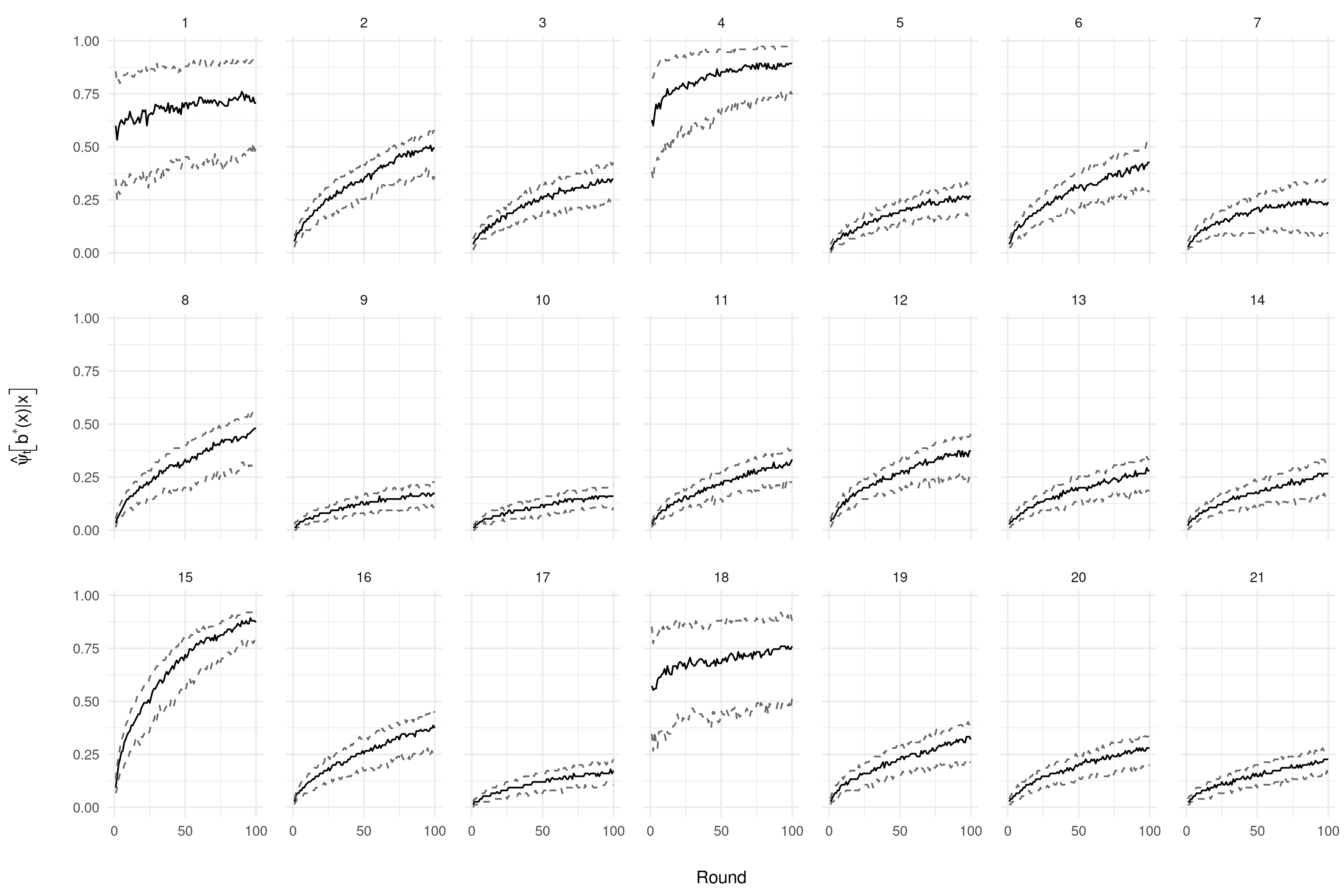
Figure 1: Convergence of BITS algorithm for SPAs

The results confirm the convergence of BITS, which holds across all contexts, each of which with a specific DGP and optimal bid. The results also show there are differences across contexts. The contexts that are more likely to happen (2, 4 and 15) often converge more quickly, which is expected since more observations are obtained per round. Since the remaining contexts happen with virtually the same probabilities, the observed differences are due to the differences in the mean and variance of rewards across arms and contexts.

An interesting exception are the contexts whose optimal bids are 0 (contexts 1, 4 and 18). Convergence for these contexts always happens quickly albeit with a larger variance. This is due to the fact that there is a corner solution. Identifying that always losing is the optimal strategy is not difficult for the algorithm; however, the need for exploration requires it to compensate for the quick accumulation of observations with losses, leading to a larger variance in $\hat{\psi}_{t}\left[\middle|b^{*}(x)|x\right]$. Nevertheless, BITS still recovers the optimal bid, showcasing that it is robust to various situations and DGPs.

Now that we verified that BITS works in practice, we proceed to compare its performance to the aforementioned alternative methods. We start by comparing their performance in minimizing regret. Figure 2 plots the evolution of the cumulative regret at each round averaged across all epochs. The solid line shows the results for the A/B test, the dash-dotted line for ETC, the dashed line for the off-the-shelf TS, and the dotted line for BITS.

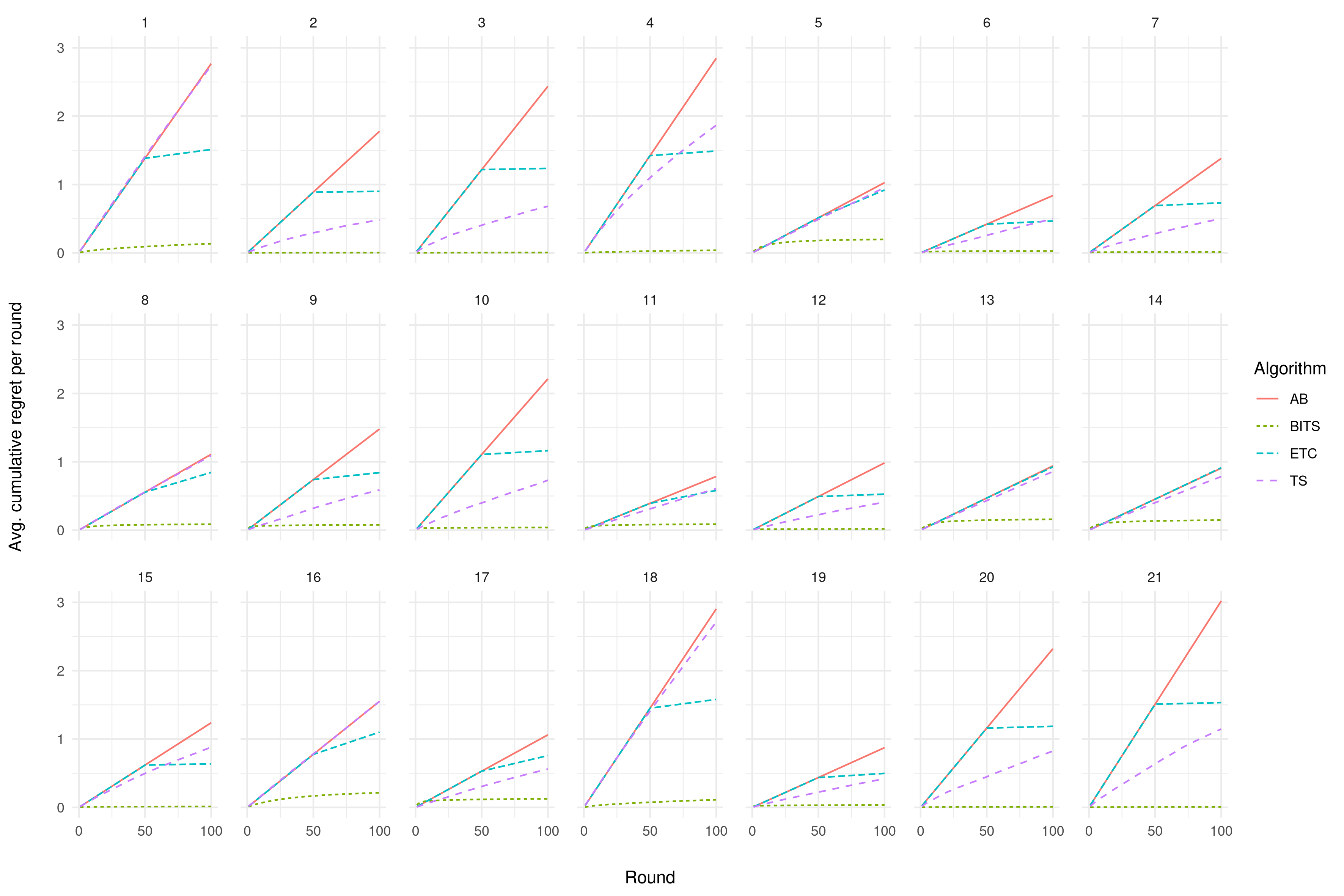
Figure 2: Evolution of regret for SPAs

Across all contexts, BITS outperforms the other methods in minimizing regret. Again this is driven by the fact BITS is the only method that not only aims at minimizing regret but also exploits the entire structure of the DGP. In. turn, AB always has the worst performance across the three competing methods. Once again, this is unsurprising: by always randomizing across all the arms in the grid, this method has constant and fixed regret per round and therefore a linear and increasing cumulative regret.

Because ETC follows AB for the first half of each epoch, their performances exactly coincide over the first half of rounds. After that, ETC computes the optimal arm based on the data collected and uses this estimate for the rest of experiment. Hence, its cumulative regret follows a piecewise linear pattern, with the second line being flatter than the first. We indeed verify this to be the case across all contexts, though the extent to which the slope of the curve decreases is a function of the number of observations, expected regret across arms and the variance of rewards. The most interesting results perhaps concern the contexts for which this decrease was minimal (5, 13 and 14). All these contexts display relatively close regret across arms, so that randomizing between arms and using an estimate seem to imply small differences in regret.

We observe that the performance of TS relative to AB and ETC varies considerably across contexts. We observe that TS has difficulties in identifying the optimal arm when it corresponds to a bid of zero (contexts 1, 4 and 18). Its ranking relative AB and ETC is context-specific. This is, once again, a result of the number of observations for each context as well as the expected regret and variance of rewards across arms.

Finally, we compare the performance of BITS to that of the other methods using the MSE. Despite being directly connected to regret, this metric directly assess the precision with which the $ATE$ is estimated. Results are shown in Table 4. We multiply the MSEs by $10^{5}$ to ease visualization.

Context	AB	ETC	TS	BITS
1	189	278	6,052	4
2	185	253	1,241	4
3	253	554	2,010	7
4	39	129	2,064	1
5	230	575	3,985	11
6	150	282	2,036	5
7	464	1,339	964	9
8	136	260	4,808	4
9	1,614	4,781	1,029	29
10	2,791	7,310	2,389	34
11	1,111	675	2,792	8
12	410	776	1,330	6
13	423	805	3,679	11
14	517	609	3,390	13
15	16	27	2,294	1
16	465	333	5,385	7
17	4,789	17,691	1,235	27
18	139	221	5,623	4
19	382	712	1,561	9
20	489	898	2,274	11
21	620	886	4,066	13

Table 4: $10^{5}\times\widehat{\text{MSE}}_{\iota}(x)$

As in the regret results, BITS outperforms the other methods across all contexts. Once again, this is not surprising: because in SPAs the $ATE$ corresponds to the optimal arm and given the results shown in Figures 1 and 2, at the end of the exercises BITS yields a very precise estimate of the $ATE$ not only because it places a high posterior probability on the true optimal arm, but also because it places relatively high probabilities on the arms that are closest to the optimal one.

The performance of BITS is usually followed by that of AB, which is also expected: the estimate from AB leverages all the data collected and is obtained with the explicit goal of minimizing MSE. By construction, we expected the performance of AB to always be better than that of ETC, which was the case across all contexts but two (11 and 16). Upon inspection, we verified that this happened because AB used outliers to estimate the $ATE$ but ETC did not, which led to a higher MSE.

Finally, TS performed worse than AB across all the contexts and its performance relative to ETC was worse in all but three contexts (7, 9 and 10). Once more, this is a function of the number of observations and expected regret and variance of rewards across arms.

6.5 FPA results

Once again we start by presenting results demonstrating convergence of BITS. Figure 3 shows the evolution of the estimated optimality probability of the true optimal arm, $\hat{\psi}_{t}\left[b^{*}(x)\middle|x\right]$. The solid line displays the median while the dashed lines show the interquartile range.

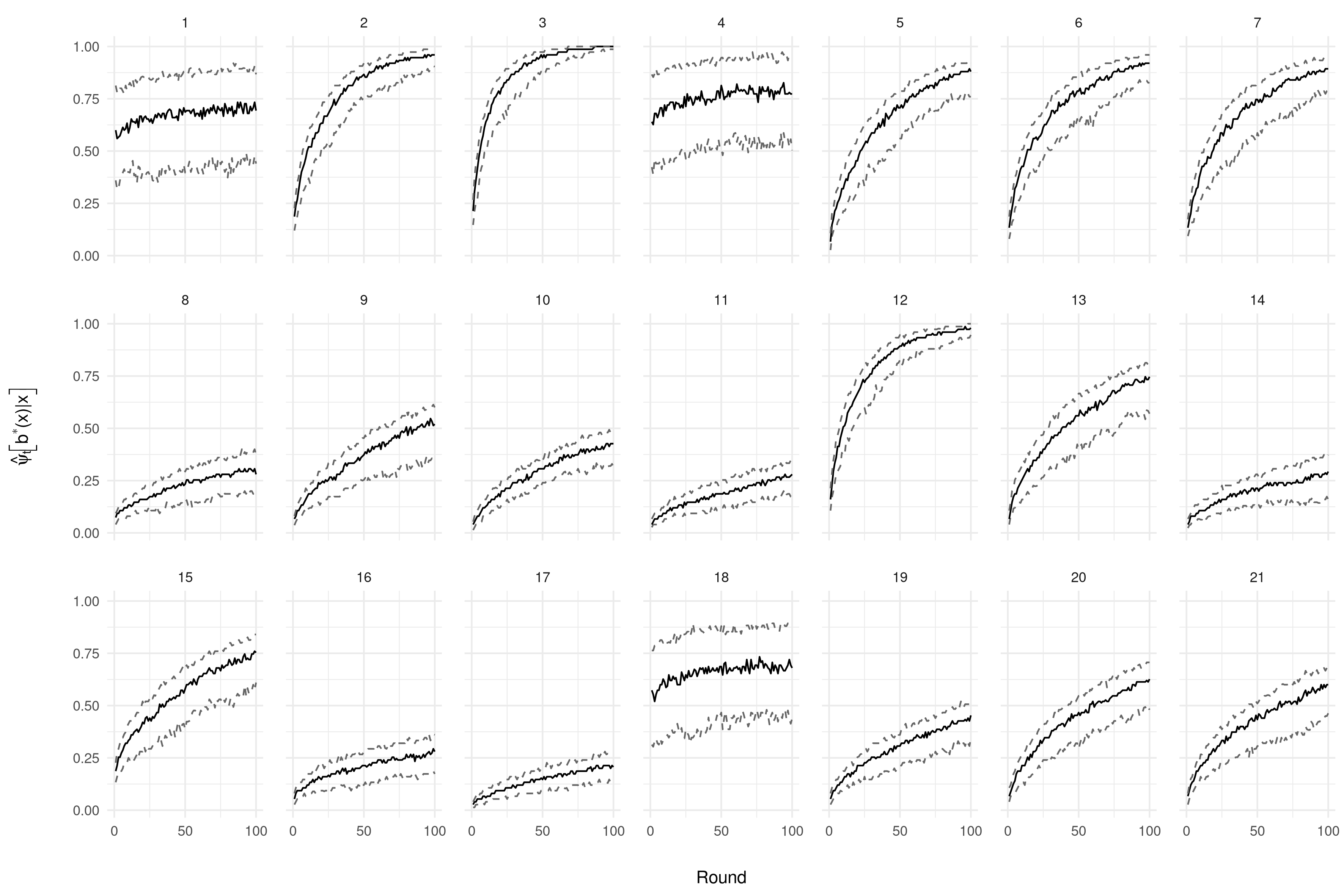
Figure 3: Convergence of BITS algorithm for FPAs

Figure 3 demonstrates that BITS correctly identifies all the optimal arms. It is useful to recognize differences in the speed of convergence across contexts. The contexts whose optimal bid is zero (1,4 and 18) display a fast but noisy convergence due to the same reasons outlined above regarding the results found for SPAs. It is interesting to note that even though contexts with a higher number of observations (2, 3 and 15) converge quickly, other contexts with relatively fewer observations converge at a comparable place. This is a consequence of the different means and variance of rewards across the different contexts.

We now compare the performance of BITS to the alternative methods we consider. We begin by comparing their performance in minimizing regret. Figure 4 shows the evolution of cumulative regret across methods and contexts averaged across epochs.

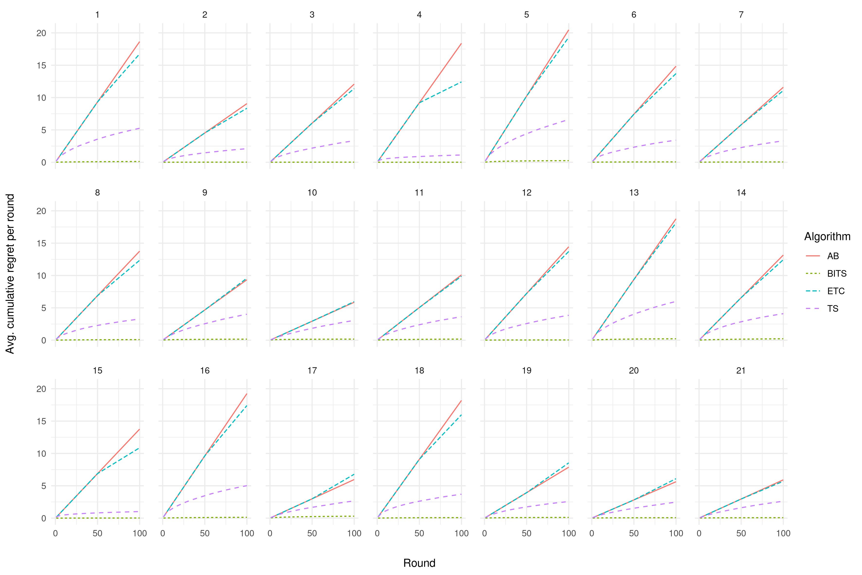
Figure 4: Evolution of regret for FPAs

As before, BITS outperforms all competing methods across all contexts. Unlike before, however, as a result of the parameters of the exercise and of the different mechanism (FPA instead of SPA), we now observe that TS always outperforms both AB and ETC. In particular, we find that TS can be very competitive with BITS in contexts 4 and 15. Since TS is simpler to implement than BITS, this demonstrates that it is possible that TS might be preferable over BITS in practice. Nevertheless, it is difficult to establish whether this is the case ex ante. Contexts 4 and 15 have a relatively larger number of observations than other contexts, but so do contexts 2 and 3, where the performance of TS is not as competitive with that of BITS. Finally, it is interesting to note that ETC does not outperform AB as starkly as before.

To verify the precision with which these different methods recover the $ATE$s, we compute MSEs as described above. Results are shown in Table 5. Notice that because the off-the-shelf TS cannot estimate $ATE$s, we only compare BITS to AB and ETC.

Context	A/B	ETC	BITS
1	139	341	32
2	800	2,842	3
3	231	505	1
4	32	34	5
5	417	1,004	10
6	192	342	3
7	1,405	2,036	8
8	224	335	39
9	2,040	4,922	39
10	10,130	4,230	34
11	1,199	2,443	48
12	1,222	4,588	2
13	3,604	14,151	14
14	640	1,515	69
15	61	41	4
16	301	363	22
17	1,433	3,514	99
18	190	447	21
19	703	1,329	22
20	806	1,769	17
21	1,024	2,658	24

Table 5: $10^{5}\times\widehat{\text{MSE}}_{\iota}(x)$

As before, BITS outperforms AB and ETC across all contexts in terms of obtaining low MSEs. It is interesting that although AB dominates ETC across the majority of contexts, as expected since it uses a larger number of observations to estimate $ATE$s, there are cases in which this is not the case (contexts 10 and 15). Upon inspecting the data we verify that this is due to the presence of outliers.

Unlike in SPAs, the estimator of $ATE$s based on BITS for FPAs does not involve solely the uncertainty over the true optimal arm. It also relies on estimating the distribution of $B_{CP}$ conditional on $x$. This added source of uncertainty impacts the performance of BITS in estimating the $ATE$s. Even though Table 5 indicates that this is not the case, we inspect this further by computing the density of the estimated $ATE$s across contexts and epochs. We use the Epanechnikov kernel with Silverman’s rule-of-thumb bandwidth to compute these estimates. Results are shown in Figure 5. The solid line is the estimated density and the vertical dashed line corresponds to the true $ATE$.

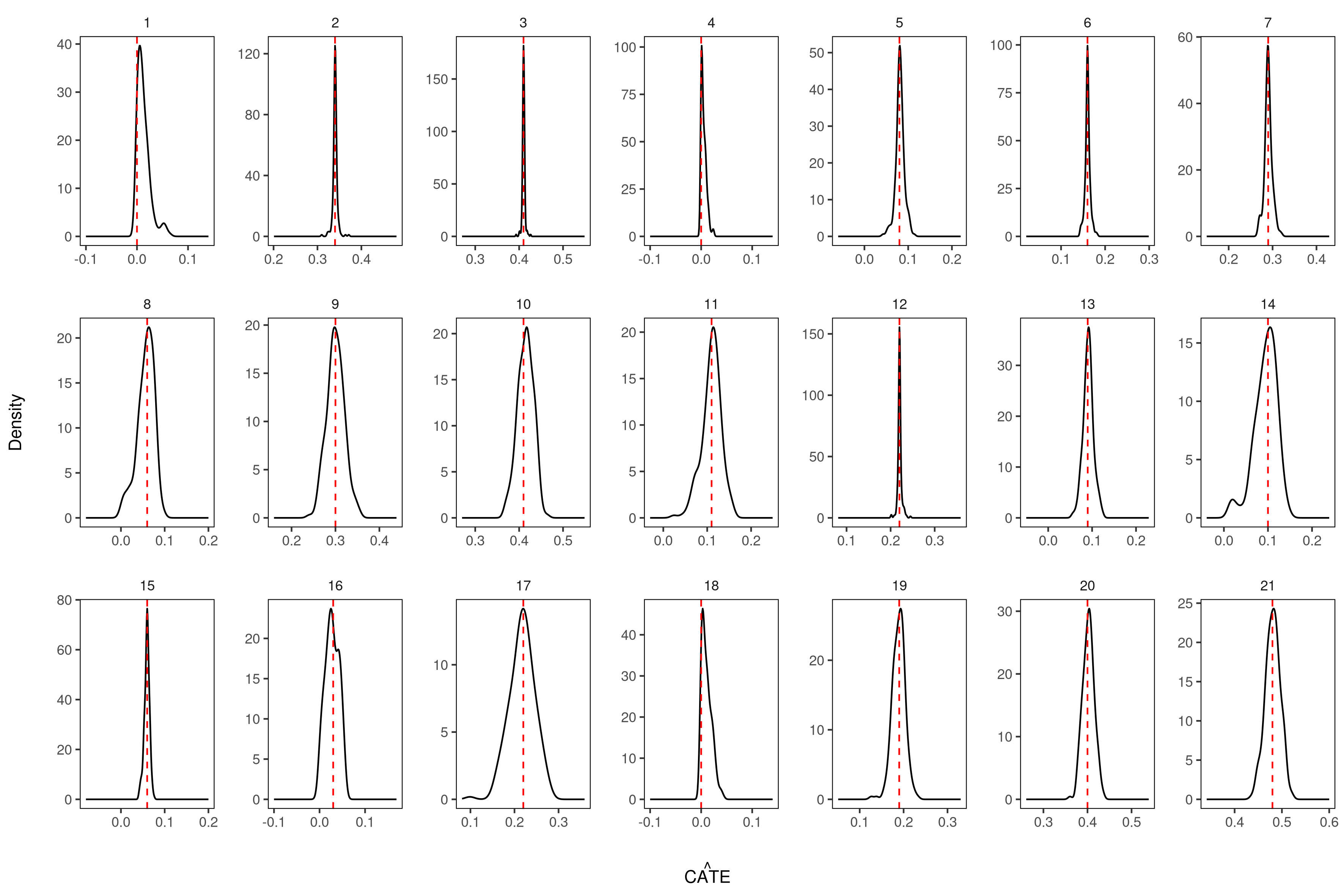
Figure 5: Density of estimate of $ATE$s from FPAs

Figure 5 shows that despite the added source of uncertainty in the estimator of the $ATE$s with FPAs, BITS succeeds in identifying the true $ATE$. This is because the density of estimates is always centered around the true $ATE$.

7 Concluding remarks

An online method to perform causal inference on RTB advertising is presented. This method leverages the theory of optimal bidding under sealed-bid SPAs and FPAs to align the twin goals of obtaining economic payoff maximization and inference on the expected effect of advertising for varying subpopulations. The algorithm is framed to solve a contextual MAB problem implemented via a modified TS that is adaptively updated via MCMC. The SPA environment is historically the most popular auction format for RTB ads and the proposed experimental design perfectly aligns the economic and inference goals of the advertiser in this environment. Extensions to the more complex FPA environment, which has become popular more recently, are also presented.

Some broader implications of the experimental design beyond RTB advertising are worth mentioning. First, the ideas presented here can be useful in other situations outside of ad auctions where there is a cost to obtaining experimental units and where managing these costs is critical for the viability of the experiment. These costs can be driven by the cost of acquiring experimental units (such as sending mailers in offline experiments, or other incentives given for experimental participation), as well as the opportunity costs of showing ex ante unproven treatments (such as new creatives or new price ranges) to users. Another implication is that, in business experiments, incorporating the firm’s payoff or profit maximization goal into the allocation and acquisition of experimental units is helpful. Examples include pricing experiments and product feature experiments for which there is a clear payoff goal to the firm from such experimentation, which can be incorporated into the MAB problem. Given the burgeoning utilization of experimentation by firms, we believe that leveraging this perspective in business experiments more broadly has value. Finally, another takeaway from the proposed approach is that it demonstrates the value of embedding experimental design in the microfoundations of the problem, which enables leveraging economic theory to make progress on running experiments more effectively. This aspect could be utilized in other settings where large-scale experimentation is feasible and where economic theory puts structure on the behavior of agents and associated outcomes. The fusing of experimental design and economic theory in this manner is a direction for our future research.

Appendix

A Proofs

A.1 Proof or Proposition 1

Proof.

To prove Proposition 1, we first rewrite equation (3):

$$\bar{\pi}(b|x) =\Pr\left\{B_{CP}\leq b\middle|x\right\}\left\{\mathbb{E}\left[Y(1)-Y(0)\middle|B_{CP}\leq b;x\right]-\mathbb{E}\left[B_{CP}\middle|B_{CP}\leq b;x\right]\right\}$$

$$=\Pr\left\{B_{CP}\leq b\middle|x\right\}\left\{\mathbb{E}\left[Y(1)-Y(0)\middle|x\right]-\mathbb{E}\left[B_{CP}\middle|B_{CP}\leq b;x\right]\right\}$$

$$=\Pr\left\{B_{CP}\leq b\middle|x\right\}\left\{ATE(x)-\mathbb{E}\left[B_{CP}\middle|B_{CP}\leq b;x\right]\right\}$$

$$=\int_{0}^{b}\left[ATE(x)-b_{CP}\right]f_{CP}(b_{CP}|x)db_{CP},$$

where the second equality follows from Assumption 1. Notice that $\bar{\pi}(b|x)$ becomes a bidder’s expected payoff from an SPA in which the bidder’s expected private value equals $ATE(x)$. Since the advertiser cannot submit negative bids, if $ATE(x)\leq 0$ the optimal bid is $b^{*}(x)=0$ because the integrand is negative and $f_{CP}(\cdot|x)>0$ in the interior of $\mathbb{R}_{+}$ due to Assumption 2. Otherwise, notice that the integrand is non-negative as long as $b(x)\leq ATE(x)$, which implies the optimal bid cannot exceed $ATE(x)$. Once again, due to Assumption 2, $f_{CP}(\cdot|x)>0$, so that $b^{*}(x)=ATE(x)$. ∎

A.2 Proof or Proposition 2

Proof.

To prove Proposition 2, we proceed as above, by rewriting equation (3):

$$\bar{\pi}(b|x) =\Pr\left\{B_{CP}\leq b\middle|x\right\}\left\{\mathbb{E}\left[Y(1)-Y(0)-b\middle|B_{CP}\leq b;x\right]\right\}$$

$$=\Pr\left\{B_{CP}\leq b\middle|x\right\}\left\{\mathbb{E}\left[Y(1)-Y(0)\middle|x\right]-b\right\}$$

$$=F_{CP}\left(b|x\right)\left\{ATE(x)-b\right\},$$

where, once again, the second equality follows from Assumption 1. If $ATE(x)\leq 0$, it is straightforward to verify that $b^{*}(x)=0$ since the advertiser cannot submit negative bids. Consider now the case where $ATE(x)>0$. The first-order condition with respect to $b$ is given by

$$CATE(x)=b+\frac{F_{CP}\left(b|x\right)}{f_{CP}\left(b|x\right)}\equiv\chi(b).$$ (A.1)

Assumption 2 ensures that $\chi(0)=0$. In addition, Assumption 2 implies that the right-hand side of equation (A.1) is monotonically increasing in $b$. Hence, $\chi(\cdot)$ is invertible, which yields a unique solution. Denoting its inverse by $\chi^{-1}(\cdot)$, the optimal bid is therefore given by $b^{*}(x)=\max\left\{0,\chi^{-1}\left[ATE(x)\right]\right\}$. ∎

A.3 Proof of Proposition 3

Proof.

To leverage the results from Russo and Van Roy, (2014) and Bubeck and Liu, (2013) we need to normalize rewards so that they are bounded by 1. Consider first the rewards for SPAs. From equation (2) we have that:

$$\pi(b) =\mathbbm{1}\left\{B_{CP}\leq b\right\}\times\left\{\left[Y(1)-Y(0)\right]-B_{CP}\right\}+Y(0)$$

$$\leq\mathbbm{1}\left\{B_{CP}\leq b\right\}\times Y(1)+Y(0)$$

$$\leq\mathbbm{1}\left\{B_{CP}\leq b\right\}\times\bar{y}_{1}+\bar{y}_{0}$$

$$\leq\bar{y}_{1}+\bar{y}_{0}$$

$$\equiv\kappa_{SPA}.$$

In turn, for FPAs equation (2) implies that:

$$\pi(b) =\mathbbm{1}\left\{B_{CP}\leq b\right\}\times\left\{\left[Y(1)-Y(0)\right]-b\right\}+Y(0)$$

$$\leq\mathbbm{1}\left\{B_{CP}\leq b\right\}\times\left[Y(1)-b\right]+Y(0)$$

$$\leq\mathbbm{1}\left\{B_{CP}\leq b\right\}\times\left(\bar{y}_{1}-b_{1}\right)+\bar{y}_{0}$$

$$\leq\bar{y}_{1}+\bar{y}_{0}-b_{1}$$

$$\equiv\kappa_{FPA}.$$

Because the proof is the same for both auction formats, we will establish the result for a constant $\kappa$, which can be either $\kappa_{SPA}$ and $\kappa_{FPA}$ as defined above.

We now use this constant to rescale regret. Define $\tilde{\pi}(b)=\frac{\pi(b)}{\kappa}$. From equations (4) and (9), we have:

$$\text{Regret}(T,\theta) =\sum_{t=1}^{T}\mathbb{E}\left\{\bar{\pi}\left[b^{*}(x_{t})\middle|x_{t}\right]-\bar{\pi}\left[b_{t}(x_{t})\middle|x_{t}\right]\middle|\theta\right\}$$

$$=\frac{\kappa}{\kappa}\sum_{t=1}^{T}\mathbb{E}\left\{\mathbb{E}\left\{\pi\left[b^{*}(x_{t})\right]\middle|x_{t}\right\}-\mathbb{E}\left\{\pi\left[b_{t}(x_{t})\right]\middle|x_{t}\right\}\middle|\theta\right\}$$

$$=\kappa\sum_{t=1}^{T}\mathbb{E}\left\{\mathbb{E}\left[\frac{\pi\left[b^{*}(x_{t})\right]}{\kappa}\middle|x_{t}\right]-\mathbb{E}\left[\frac{\pi\left[b_{t}(x_{t})\right]}{\kappa}\middle|x_{t}\right]\middle|\theta\right\}$$

$$=\kappa\sum_{t=1}^{T}\mathbb{E}\left\{\mathbb{E}\left\{\tilde{\pi}\left[b^{*}(x_{t})\right]\middle|x_{t}\right\}-\mathbb{E}\left\{\tilde{\pi}\left[b_{t}(x_{t})\right]\middle|x_{t}\right\}\middle|\theta\right\}$$

$$\equiv\kappa\sum_{t=1}^{T}\mathbb{E}\left\{\overline{\tilde{\pi}}\left[b^{*}(x_{t})\middle|x_{t}\right]-\overline{\tilde{\pi}}\left[b_{t}(x_{t})\middle|x_{t}\right]\middle|\theta\right\}$$

$$\equiv\kappa\times\widetilde{\text{Regret}}(T,\theta).$$ (A.2)

Taking the expectations over $\theta$ and equation (10), we obtain

$$\text{BayesRegret}(T) \equiv\kappa\times\widetilde{\text{BayesRegret}}(T).$$

We will obtain bounds on this rescaled regret metric, which will then yield the final result. First, notice that:

$$\widetilde{\text{BayesRegret}}(T)\leq\mathbb{E}\left[\sum_{t=1}^{T}\sum_{r=1}^{R}\overline{\tilde{\pi}}\left[b_{r}^{*}(x_{t})\middle|x_{t}\right]-\overline{\tilde{\pi}}\left[b_{r,t}(x_{t})\middle|x_{t}\right]\right].$$ (A.3)

Let $W_{x,t}(b)$ be a random variable that is measurable with respect to the $\sigma$-algebra induced by $H_{t-1}$, and let $x_{t}$ be the context in round $t$. From Proposition 1 of Russo and Van Roy, (2014), we know that:

$$\mathbb{E}\left\{W_{x_{t},t}\left[b_{r}^{*}(x_{t})\right]\middle|H_{t-1}\right\}=\mathbb{E}\left\{W_{x_{t},t}\left[b_{r,t}(x_{t})\right]\middle|H_{t-1}\right\}.$$

Hence, we have that:

$$\mathbb{E}\left\{\overline{\tilde{\pi}}\left[b_{r}^{*}(x_{t})\middle|x_{t}\right]-\overline{\tilde{\pi}}\left[b_{r,t}(x_{t})\middle|x_{t}\right]\right\} =\mathbb{E}\left[\mathbb{E}\left\{\overline{\tilde{\pi}}\left[b_{r}^{*}(x_{t})\middle|x_{t}\right]-\overline{\tilde{\pi}}\left[b_{r,t}(x_{t})\middle|x_{t}\right]\middle|H_{t-1}\right\}\right]$$

$$=\mathbb{E}\left[\mathbb{E}\left\{\overline{\tilde{\pi}}\left[b_{r}^{*}(x_{t})\middle|x_{t}\right]-W_{x_{t},t}\left[b_{r}^{*}(x_{t})\right]\middle|H_{t-1}\right\}\right]$$

$$\qquad+\mathbb{E}\left[\mathbb{E}\left\{W_{x_{t},t}\left[b_{r,t}(x_{t})\right]-\overline{\tilde{\pi}}\left[b_{r,t}(x_{t})\middle|x_{t}\right]\middle|H_{t-1}\right\}\right]$$

$$=\mathbb{E}\left\{\overline{\tilde{\pi}}\left[b_{r}^{*}(x_{t})\middle|x_{t}\right]-W_{x_{t},t}\left[b_{r}^{*}(x_{t})\right]\right\}$$

$$\qquad+\mathbb{E}\left\{W_{x_{t},t}\left[b_{r,t}(x_{t})\right]-\overline{\tilde{\pi}}\left[b_{r,t}(x_{t})\middle|x_{t}\right]\right\}.$$

Therefore,

$$\begin{split}\widetilde{\text{BayesRegret}}(T)&\leq\mathbb{E}\left\{\sum_{t=1}^{T}\sum_{r=1}^{R}\overline{\tilde{\pi}}\left[b_{r}^{*}(x_{t})\middle|x_{t}\right]-W_{x_{t},t}\left[b_{r}^{*}(x_{t})\right]\right\}\\ &\qquad+\mathbb{E}\left\{\sum_{t=1}^{T}\sum_{r=1}^{R}W_{x_{t},t}\left[b_{r,t}(x_{t})\right]-\overline{\tilde{\pi}}\left[b_{r,t}(x_{t})\middle|x_{t}\right]\right\}.\end{split}$$ (A.4)

We now consider the two terms in the right-hand side of (A.4) separately and provide upper bounds for them. To this end, define:

$$W_{x,t}(b_{r})=\min\left\{1,\widehat{\tilde{\pi}}_{r,x,t-1}+\sqrt{\frac{\log\left(\frac{TR}{N_{r,x,t-1}P}\right)\mathbbm{1}\left\{\frac{TR}{N_{r,x,t-1}P}\geq 1\right\}}{N_{r,x,t-1}}}\right\}$$

and

$$\tilde{W}_{x,t}(b_{r})=\widehat{\tilde{\pi}}_{r,x,t-1}+\sqrt{\frac{\log\left(\frac{\eth}{N_{r,x,t-1}RP}\right)\mathbbm{1}\left\{\frac{\eth}{N_{r,x,t-1}RP}\geq 1\right\}}{N_{r,x,t-1}}},$$

where we have that $\eth>0$, $\widehat{\tilde{\pi}}_{r,x,t-1}=\frac{1}{N_{r,x,t-1}}\sum_{\tau=1}^{t-1}\mathbbm{1}\left\{b_{\tau}-b_{r},x_{\tau}=x\right\}\pi_{\tau}(b_{r})$ and $N_{r,x,t-1}=\sum_{\tau=1}^{t-1}\mathbbm{1}\left\{b_{\tau}=b_{r},x_{\tau}=x\right\}$. Hence, $N_{r,x,t-1}$ is the number of times $b_{r}$ is submitted when the context is $x$ over the first $t-1$ periods, and $\widehat{\tilde{\pi}}_{r,x,t-1}$ is an UCB function.

Using Theorem 1 of Bubeck and Liu, (2013), we know that, for any $r$, $t$ and $x$, we have that

$$\mathbb{E}\left[\max\left\{\overline{\tilde{\pi}}\left[b_{r}\middle|x\right]-\tilde{W}_{x,t}(b_{r}),0\right\}\right]\leq 6\sqrt{\frac{RP}{\eth}}.$$

Letting $\eth=TR^{2}$, we get:

$$\mathbb{E}\left[\max\left\{\overline{\tilde{\pi}}\left[b_{r}\middle|x\right]-W_{x,t}(b_{r}),0\right\}\right]\leq\mathbb{E}\left[\max\left\{\overline{\tilde{\pi}}\left[b_{r}\middle|x\right]-\tilde{W}_{x,t}(b_{r}),0\right\}\right]\leq 6\sqrt{\frac{P}{TR}}.$$

Finally, applying this result to $b_{r}^{*}(\cdot)$, and adding over $t$ and $r$ yields:

$$\mathbb{E}\left\{\sum_{t=1}^{T}\sum_{r=1}^{R}\overline{\tilde{\pi}}\left[b_{r}^{*}(x_{t})\middle|x_{t}\right]-W_{x,t}\left[b_{r}^{*}(x_{t})\right]\right\}\leq 6\sqrt{PRT}\leq 6\sqrt{PRT\log(R)},$$ (A.5)

which bounds the first term in the right-hand side of (A.4).

We now address the second term. First, note that:

$$\mathbb{E}\left\{\sum_{t=1}^{T}\sum_{r=1}^{R}W_{x_{t},t}\left[b_{r,t}(x_{t})\right]-\overline{\tilde{\pi}}\left[b_{r,t}(x_{t})\middle|x_{t}\right]\right\} =\sum_{t=1}^{T}\sum_{r=1}^{R}\mathbb{E}\left\{W_{x_{t},t}\left[b_{r,t}(x_{t})\right]-\overline{\tilde{\pi}}\left[b_{r,t}(x_{t})\middle|x_{t}\right]\right\}$$

$$=\sum_{t=1}^{T}\mathbb{E}\left\{W_{x_{t},t}\left[b_{t}(x_{t})\right]-\overline{\tilde{\pi}}\left[b_{t}(x_{t})\middle|x_{t}\right]\right\}.$$

If $PR\geq T$, we have that

$$\sum_{t=1}^{T}\mathbb{E}\left\{W_{x_{t},t}\left[b_{t}(x_{t})\right]-\overline{\tilde{\pi}}\left[b_{t}(x_{t})\middle|x_{t}\right]\right\} \leq T\leq 12\sqrt{PRT\log(R)}.$$ (A.6)

Consider now the case in which $PR\leq T$. From Theorem 1 of Bubeck and Liu, (2013) and setting $\eth=T$, we know that

$$\sum_{t=1}^{T}\mathbb{E}\left\{\tilde{W}_{x_{t},t}\left[b_{t}(x_{t})\right]-\overline{\tilde{\pi}}\left[b_{t}(x_{t})\middle|x_{t}\right]\right\}\leq 8\sqrt{PRT}\leq 8\sqrt{PRT\log(R)}.$$ (A.7)

Now notice that

$$W_{x,t}(b_{r}) \leq\min\left\{1,\widehat{\tilde{\pi}}_{r,x,t-1}+\sqrt{\frac{\log\left(\frac{T}{N_{r,x,t-1}RP}\right)\mathbbm{1}\left\{\frac{TR}{N_{r,x,t-1}P}\geq 1\right\}+\log(R^{2})}{N_{r,x,t-1}}}\right\}$$

$$\leq\tilde{W}_{x,t}(b_{r})+\min\left\{\sqrt{\frac{2\log(K)}{N_{r,x,t-1}}},1\right\},$$

so that

$$\begin{split}&\sum_{t=1}^{T}\mathbb{E}\left\{W_{x_{t},t}\left[b_{t}(x_{t})\right]-\overline{\tilde{\pi}}\left[b_{t}(x_{t})\middle|x_{t}\right]\right\}\leq 8\sqrt{PRT}\\ &\qquad\qquad\qquad\qquad\qquad+\sum_{t=1}^{T}\sum_{r=1}^{R}\sum_{x\in\mathbb{X}}\mathbb{E}\left[\min\left\{\sqrt{\frac{2\log(K)}{N_{r,x,t-1}}},1\right\}\mathbbm{1}\left\{b_{t}=b_{r},x_{t}=x\right\}\right].\end{split}$$ (A.8)

From Proposition 1 of Russo and Van Roy, (2014), we know that

$$\sum_{t=1}^{T}\sum_{r=1}^{R}\sum_{x\in\mathbb{X}}\mathbb{E}\left[\min\left\{\sqrt{\frac{2\log(K)}{N_{r,x,t-1}}},1\right\}\mathbbm{1}\left\{b_{t}=b_{r},x_{t}=x\right\}\right]\leq 4\sqrt{PRT\log(R)}.$$ (A.9)

Plugging (A.9) into (A.8) yields

$$\sum_{t=1}^{T}\mathbb{E}\left\{W_{x_{t},t}\left[b_{t}(x_{t})\right]-\overline{\tilde{\pi}}\left[b_{t}(x_{t})\middle|x_{t}\right]\right\}\leq 12\sqrt{PRT\log(R)},$$

which is equivalent to the result in (A.6).

Finally, plugging (A.5) and (A.6) into (A.4) implies that

$$\widetilde{\text{BayesRegret}}(T)\leq 18\sqrt{PRT\log(R)}$$

and along with equation (A.3) that

$$\text{BayesRegret}(T)\leq 18\kappa\sqrt{PRT\log(R)},$$

establishing the result. ∎

B Gibbs sampling procedure

We now present in detail the procedure we discussed in Section 5.3.3 to obtain draws from the posterior distribution of the vector of parameters, $\theta$. The procedure closely follows the method given in Section 14.11 of Chan et al., (2020). We will proceed as follows. We begin by describing the method for SPAs. Then, we briefly discuss the method for FPAs since it only requires a slight change to the algorithm for SPAs. Both these approaches assume, for simplicity, that $\rho=0$, so we conclude by showing how the approach can be adapted to relax this assumption.

B.1 Application to SPAs

Step 1: drawing missing values

The first step in our procedure is to draw the missing values from our data conditional on the available data, $H_{t}$, and a given vector of parameters, $\theta$. We begin by drawing the missing values $\left\{\log B_{CP,i}\right\}_{i:D_{i}=0}$. Given $\left(H_{t},\theta\right)$ and under (12), we have:

$$\log B_{CP,i}^{miss}\Big{|}D_{i}=0,\log Y_{i},\log\bar{B}_{CP,i},\log b_{i},X_{i},\theta\overset{d}{=}$$

$$\log B_{CP,i}^{miss}\Big{|}D_{i}=0,\log b_{i},X_{i},\delta_{CP},\sigma_{CP}^{2}\sim TN\left(X_{i}^{\prime}\delta_{CP},\sigma_{CP}^{2},\log b_{i},+\infty\right),$$ (B.1)

where $\overset{d}{=}$ means equality in distribution and $TN\left(\delta_{*},\sigma_{*}^{2},l,u\right)$ denotes the truncated normal distribution with mean $\delta_{*}$, variance $\sigma_{*}^{2}$, lower truncation at $l$ and upper truncation at $u$.

Now we proceed to draw the missing values $\left\{\log Y_{i}(1)\right\}_{i:D_{i}=0}$ and $\left\{\log Y_{i}(0)\right\}_{i:D_{i}=1}$. Given $\left(H_{t},\theta\right)$ and under (12), it follows that:

$$\log Y_{i}^{miss}(1)\Big{|}D_{i}=0,\log Y_{i},\log\bar{B}_{CP,i},\log b_{i},X_{i},\theta\overset{d}{=}$$

$$\log Y_{i}^{miss}(1)\Big{|}D_{i}=0,X_{i},\delta_{1},\sigma_{1}^{2}\sim N\left(X_{i}^{\prime}\delta_{1},\sigma_{1}^{2}\right)$$ (B.2)

and,

$$\log Y_{i}^{miss}(0)\Big{|}D_{i}=1,\log Y_{i},\log\bar{B}_{CP,i},\log b_{i},X_{i},\theta\overset{d}{=}$$

$$\log Y_{i}^{miss}(0)\Big{|}D_{i}=1,X_{i},\delta_{0},\sigma_{0}^{2}\sim N\left(X_{i}^{\prime}\delta_{0},\sigma_{0}^{2}\right).$$ (B.3)

Now, defining,

$$\delta_{i}^{miss}=D_{i}\times X_{i}^{\prime}\delta_{0}+(1-D_{i})\times X_{i}^{\prime}\delta_{1}$$ (B.4)

$$\sigma_{i}^{2,miss}=D_{i}\times\sigma_{0}^{2}+(1-D_{i})\times\sigma_{1}^{2},$$ (B.5)

we can combine (B.1) and (B.1) into:

$$\log Y_{i}^{miss}\Big{|}\log Y_{i},D_{i},\log\bar{B}_{CP,i},\log b_{i},X_{i},\theta\overset{d}{=}$$

$$\log Y_{i}^{miss}\Big{|}D_{i},X_{i},\delta_{1},\delta_{0},\sigma_{1}^{2},\sigma_{0}^{2}\sim N\left(\delta_{i}^{miss},\sigma_{i}^{2,miss}\right).$$ (B.6)

Step 2: augmenting the data

Given a draw from the distributions given above, $\left\{\log Y_{i}^{miss},\log B_{CP,i}^{miss}\right\}$, we can construct the “complete” data implied by that draw of the Markov chain:

$$\begin{split}&\log\tilde{Y}_{i}(1)=D_{i}\log Y_{i}+(1-D_{i})\log Y_{i}^{miss}\\ &\log\tilde{Y}_{i}(0)=D_{i}\log Y_{i}^{miss}+(1-D_{i})\log Y_{i}\\ &\log\tilde{B}_{CP,i}=D_{i}\log\bar{B}_{CP,i}+(1-D_{i})\log B_{CP,i}^{miss}.\end{split}$$ (B.7)

Step 3: drawing from posterior distributions

The last step is to draw a new vector of parameters from the posterior distribution given the augmented data. We stack all these data by the end of round $t$ in the following $N_{t}\times 1$ vectors: $\log\tilde{Y}_{t}(1)$, $\log\tilde{Y}_{t}(0)$, $\log\tilde{B}_{CP,t}$, $D_{t}$ and $\log b_{t}$. We also use the $N_{t}\times P$ matrix $X_{t}$, whose $i^{\text{th}}$ row is the vector $X_{i}^{\prime}$, and collect them all in the complete data set $\tilde{H}_{t}\equiv\left[\log\tilde{Y}_{t}(1),\log\tilde{Y}_{t}(0),\log\tilde{B}_{CP,t}\log b_{t},D_{t},X_{t}\right]$. Finally, let the $(q-1)^{\text{th}}$ draw of the parameters be $\theta^{(q-1)}$. Given the structure of the model, it then follows that the full conditional distributions of $\sigma^{2,(q)}\equiv\left[\sigma_{1}^{2,(q)},\sigma_{0}^{2,(q)},\sigma_{CP}^{2,(q)}\right]^{\prime}$ are:

$$\begin{split}&\sigma_{CP}^{2,(q)}\Big{|}\theta^{(q-1)},\theta_{\text{prior}},\tilde{H}_{t}\>\overset{d}{=}\>\sigma_{CP}^{2,(q)}\Big{|}\log\tilde{B}_{CP,t},X_{t},\mu_{{\delta}_{CP}},A_{CP},\alpha_{CP},\beta_{CP}\\ &\quad\sim\Gamma\left(\alpha_{CP}+\frac{N_{t}}{2},\beta_{CP}+\frac{1}{2}\left[\left(\log\tilde{B}_{CP,t}-X_{t}\hat{\delta}_{CP,t}\right)^{\prime}\left(\log\tilde{B}_{CP,t}-X_{t}\hat{\delta}_{CP,t}\right)\right.\right.\\ &\qquad+\left.\left.\left(\hat{\delta}_{CP,t}-\mu_{\delta_{CP}}\right)^{\prime}X_{t}^{\prime}X_{t}\left(A_{CP}+X_{t}^{\prime}X_{t}\right)^{-1}A_{CP}\left(\hat{\delta}_{CP,t}-\mu_{\delta_{CP}}\right)\right]\right),\end{split}$$ (B.8)

$$\begin{split}&\sigma_{1}^{2,(q)}\Big{|}\theta^{(q-1)},\theta_{\text{prior}},\tilde{W}_{t}\>\overset{d}{=}\>\sigma_{1}^{2,(q)}\Big{|}\log\tilde{Y}_{t}(1),X_{t},\mu_{{\delta}_{1}},A_{1},\alpha_{1},\beta_{1}\\ &\quad\sim\Gamma\left(\alpha_{1}+\frac{N_{t}}{2},\beta_{1}+\frac{1}{2}\left[\left(\log\tilde{Y}_{t}(1)-X_{t}\hat{\delta}_{1,t}\right)^{\prime}\left(\log\tilde{Y}_{t}(1)-X_{t}\hat{\delta}_{1,t}\right)\right.\right.\\ &\qquad+\left.\left.\left(\hat{\delta}_{1,t}-\mu_{\delta_{1}}\right)^{\prime}X_{t}^{\prime}X_{t}\left(A_{1}+X_{t}^{\prime}X_{t}\right)^{-1}A_{1}\left(\hat{\delta}_{1,t}-\mu_{\delta_{1}}\right)\right]\right)\end{split}$$ (B.9)

and

$$\begin{split}&\sigma_{0}^{2,(q)}\Big{|}\theta^{(q-1)},\theta_{\text{prior}},\tilde{W}_{t}\>\overset{d}{=}\>\sigma_{0}^{2,(q)}\Big{|}\log\tilde{Y}_{t}(0),X_{t},\mu_{{\delta}_{0}},A_{0},\alpha_{0},\beta_{0}\\ &\quad\sim\Gamma\left(\alpha_{0}+\frac{N_{t}}{2},\beta_{0}+\frac{1}{2}\left[\left(\log\tilde{Y}_{t}(0)-X_{t}\hat{\delta}_{0,t}\right)^{\prime}\left(\log\tilde{Y}_{t}(0)-X_{t}\hat{\delta}_{0,t}\right)\right.\right.\\ &\qquad+\left.\left.\left(\hat{\delta}_{0,t}-\mu_{\delta_{0}}\right)^{\prime}X_{t}^{\prime}X_{t}\left(A_{0}+X_{t}^{\prime}X_{t}\right)^{-1}A_{0}\left(\hat{\delta}_{0,t}-\mu_{\delta_{0}}\right)\right]\right),\end{split}$$ (B.10)

where

$$\begin{split}&\hat{\delta}_{CP,t}=\left(X_{t}^{\prime}X_{t}\right)^{-1}X_{t}^{\prime}\log\tilde{B}_{CP,t}\\ &\hat{\delta}_{1,t}=\left(X_{t}^{\prime}X_{t}\right)^{-1}X_{t}^{\prime}\log\tilde{Y}_{t}(1)\\ &\hat{\delta}_{0,t}=\left(X_{t}^{\prime}X_{t}\right)^{-1}X_{t}^{\prime}\log\tilde{Y}_{t}(0).\end{split}$$ (B.11)

Given $\sigma^{2,(q)}$, it follows that

$$\begin{split}&\delta_{CP}^{(q)}\Big{|}\sigma^{2,(q)},\delta_{1}^{(q-1)},\delta_{0}^{(q-1)},\delta_{CP}^{(q-1)},\theta_{\text{prior}},\tilde{W}_{t}\>\overset{d}{=}\>\delta_{CP}^{(q)}\Big{|}\sigma_{CP}^{2,(q)},\log\tilde{B}_{CP,t},X_{t},\mu_{{\delta}_{CP}},A_{CP}\\ &\quad\sim N\left(\left(A_{CP}+X_{t}^{\prime}X_{t}\right)^{-1}\left(X_{t}^{\prime}\log\tilde{B}_{CP,t}+A_{CP}\mu_{{\delta}_{CP}}\right),\sigma_{CP}^{2,(q)}\left(A_{CP}+X_{t}^{\prime}X_{t}\right)^{-1}\right),\end{split}$$ (B.12)

$$\begin{split}&\delta_{1}^{(q)}\Big{|}\sigma^{2,(q)},\delta_{1}^{(q-1)},\delta_{0}^{(q-1)},\delta_{CP}^{(q-1)},\theta_{\text{prior}},\tilde{W}_{t}\>\overset{d}{=}\>\delta_{1}^{(q)}\Big{|}\sigma_{1}^{2,(q)},\log\tilde{Y}_{t}(1),X_{t},\mu_{{\delta}_{1}},A_{1}\\ &\quad\sim N\left(\left(A_{1}+X_{t}^{\prime}X_{t}\right)^{-1}\left(X_{t}^{\prime}\log\tilde{Y}_{t}(1)+A_{1}\mu_{{\delta}_{1}}\right),\sigma_{1}^{2,(q)}\left(A_{1}+X_{t}^{\prime}X_{t}\right)^{-1}\right)\end{split}$$ (B.13)

and

$$\begin{split}&\delta_{0}^{(q)}\Big{|}\sigma^{2,(q)},\delta_{1}^{(q-1)},\delta_{0}^{(q-1)},\delta_{CP}^{(q-1)},\theta_{\text{prior}},\tilde{W}_{t}\>\overset{d}{=}\>\delta_{0}^{(q)}\Big{|}\sigma_{0}^{2,(q)},\log\tilde{Y}_{t}(0),X_{t},\mu_{{\delta}_{0}},A_{0}\\ &\quad\sim N\left(\left(A_{0}+X_{t}^{\prime}X_{t}\right)^{-1}\left(X_{t}^{\prime}\log\tilde{Y}_{t}(0)+A_{0}\mu_{{\delta}_{0}}\right),\sigma_{0}^{2}\left(A_{0}+X_{t}^{\prime}X_{t}\right)^{-1}\right).\end{split}$$ (B.14)

B.2 Application to FPAs

We need to adjust the Gibbs sampling procedure for FPAs due to the different data that are collected. In particular, we assume that $B_{CP}$ is always missing. As we noted in Section 5.3.3, this induces a Probit structure to $D$, which we leverage to recover the parameters of the distribution of $B_{CP}$. To do this, instead of embedding the Bayesian approach to the Tobit model by Chib, (1992) in the BITS algorithm, we use the Bayesian approach to a Probit model introduced by Albert and Chib, (1993).

This necessitates two changes to the Gibbs sampling procedure. First, we have to impose the normalization $\sigma_{CP}^{2}=1$. Second, we also have to draw the missing values $\left\{\log B_{CP,i}\right\}_{i:D_{i}=1}$ in addition to drawing $\left\{\log B_{CP,i}\right\}_{i:D_{i}=0}$ according to (B.1) with $\sigma_{CP}^{2}=1$. More concretely, we have that

$$\log B_{CP,i}^{miss}\Big{|}D_{i}=1,\log Y_{i},\log\bar{B}_{CP,i},\log b_{i},X_{i},\theta\overset{d}{=}$$

$$\log B_{CP,i}^{miss}\Big{|}D_{i}=1,\log b_{i},X_{i},\delta_{CP}\sim TN\left(X_{i}^{\prime}\delta_{CP},1,-\infty,\log b_{i}\right).$$ (B.15)

Hence, instead of creating the variable $\log\tilde{B}_{CP,i}$ according to equation (B.7), we equal it to $\log B_{CP,i}^{miss}$ for all $i$. Other than these two modifications, the rest of the procedure remains unchanged.

B.3 Gibbs sampling when potential outcomes are correlated

We now present a more general Gibbs sampling procedure that accommodates the possibility that $\rho\neq 0$. When $\rho\neq 0$, the missing values $\log Y_{i}^{miss}$ depend on the observed values $\log Y_{i}$ even conditional on $D_{i}$, which requires us to change the priors and the procedure accordingly. We now present these adaptations in detail.

Changing prior distributions

For $k\in\left\{1,0\right\}$ we replace (15) with

$$\begin{split}&\Sigma^{-1}\equiv\begin{bmatrix}\sigma_{1}^{2}&\rho\sigma_{1}\sigma_{0}\\ \rho\sigma_{1}\sigma_{0}&\sigma_{0}^{2}\end{bmatrix}^{-1}\sim\mathcal{W}\left(\nu,\Xi^{-1}\right)\\ &\delta\equiv\text{vec}(\Delta)=\begin{bmatrix}\delta_{1}\\ \delta_{0}\end{bmatrix}\sim N\left(\mu_{\delta},\Sigma\otimes A_{\delta}^{-1}\right)\end{split}$$ (B.16)

where $\mathcal{W}\left(\cdot,\cdot\right)$ denotes the Wishart distribution, $\nu$ is a non-negative scalar, $\Xi$ is a $2\times 2$ matrix, $\mu_{\delta}=\left[\mu_{\delta_{1}}^{\prime},\mu_{\delta_{0}}^{\prime}\right]^{\prime}$ is a $2P\times 1$ vector and $A_{\delta}$ is a $P\times P$ matrix. We will also use the following $P\times 2$ matrix: $M_{\delta}\equiv\left[\mu_{\delta_{1}},\mu_{\delta_{0}}\right]$.

Drawing missing potential outcomes and augmenting the data

Instead of (B.1) and (B.1) it now follows that:

$$\log Y_{i}^{miss}(1)\Big{|}D_{i}=0,\log Y_{i},\log\bar{B}_{CP,i},\log b_{i},X_{i},\theta\overset{d}{=}$$

$$\log Y_{i}^{miss}(1)\Big{|}D_{i}=0,\log Y_{i},X_{i},\delta_{1},\delta_{0},\Sigma\sim N\left(X_{i}^{\prime}\delta_{1}+\frac{\rho\sigma_{1}}{\sigma_{0}}\left(\log Y_{i}-X_{i}^{\prime}\delta_{0}\right),\left(1-\rho^{2}\right)\sigma_{1}^{2}\right)$$ (B.17)

and

$$\log Y_{i}^{miss}(0)\Big{|}D_{i}=1,\log Y_{i},\log\bar{B}_{CP,i},\log b_{i},X_{i},\theta\overset{d}{=}$$

$$\log Y_{i}^{miss}(0)\Big{|}D_{i}=1,\log Y_{i},X_{i},\delta_{1},\delta_{0},\Sigma\sim N\left(X_{i}^{\prime}\delta_{0}+\frac{\rho\sigma_{0}}{\sigma_{1}}\left(\log Y_{i}-X_{i}^{\prime}\delta_{1}\right),\left(1-\rho^{2}\right)\sigma_{0}^{2}\right),$$ (B.18)

while (B.1) and (B.2) remain the same. We can redefine $\delta_{i}^{miss}$ and $\sigma_{i}^{2,miss}$ as

$$\delta_{i}^{miss}=D_{i}\left(X_{i}^{\prime}\delta_{0}+\frac{\rho\sigma_{0}}{\sigma_{1}}\left(\log Y_{i}-X_{i}^{\prime}\delta_{1}\right)\right)+(1-D_{i})\left(X_{i}^{\prime}\delta_{1}+\frac{\rho\sigma_{1}}{\sigma_{0}}\left(\log Y_{i}-X_{i}^{\prime}\delta_{0}\right)\right)$$ (B.19)

and

$$\sigma_{i}^{2,miss}=\left(1-\rho^{2}\right)\left[D_{i}\sigma_{0}^{2}+(1-D_{i})\sigma_{1}^{2}\right],$$ (B.20)

respectively, and combine them into

$$\log Y_{i}^{miss}\Big{|}\log Y_{i},D_{i},X_{i},\delta,\Sigma\sim N\left(\delta_{i}^{miss},\sigma_{i}^{2,miss}\right).$$ (B.21)

The completion process in (B.7) remains unchanged.

Drawing from posterior distribution

We once again condition on the “complete” data, $\tilde{H}_{t}$, and on the parameters of the prior distributions. In addition to the previously defined objects, we will also use the following $N_{t}\times 2$ matrix, $\log\tilde{Y}_{PO,t}\equiv\left[\log\tilde{Y}_{t}(1),\log\tilde{Y}_{t}(0)\right]$, as well as

$$\tilde{\Delta}_{t}=\left(X_{t}^{\prime}X_{t}+A_{\delta}\right)^{-1}\left(X_{t}^{\prime}\log\tilde{Y}_{PO,t}+A_{\delta}M_{\delta}\right)$$ (B.22)

and

$$SSR_{t}=\left(\log\tilde{Y}_{PO,t}-X_{t}\tilde{\Delta}_{t}\right)^{\prime}\left(\log\tilde{Y}_{PO,t}-X_{t}\tilde{\Delta}_{t}\right)+\left(\tilde{\Delta}_{t}-M_{\delta}\right)^{\prime}A_{\delta}\left(\tilde{\Delta}_{t}-M_{\delta}\right).$$ (B.23)

To draw new values for $\sigma_{CP}^{2}$ (for SPAs only) and $\delta_{CP}$ we still utilize expressions (B.8) and (B.12), respectively. To draw new values for $\Sigma$ and $\delta$, we now leverage the following results:

$$\begin{split}&\Sigma^{-1,(q)}\Big{|}\theta^{(q-1)},\theta_{\text{prior}},\tilde{W}_{t}\>\overset{d}{=}\>\Sigma^{-1,(q)}\Big{|}\log\tilde{Y}_{PO,t},X_{t},\nu,\Xi,\mu_{\delta},A_{\delta}\\ &\qquad\sim\mathcal{W}\left(\nu+N_{t},\left(\Xi+SSR_{t}\right)^{-1}\right)\end{split}$$ (B.24)

and

$$\begin{split}&\delta^{(q)}\Big{|}\Sigma^{(q)},\sigma_{CP}^{2,(q)},\delta^{(q-1)},\delta_{CP}^{(q-1)},\theta_{\text{prior}},\tilde{W}_{t}\>\overset{d}{=}\>\delta^{(q)}\Big{|}\Sigma^{(q)},\log\tilde{Y}_{PO,t},X_{t},\mu_{\delta},A_{\delta}\\ &\qquad\sim N\left(\text{vec}\left(\tilde{\Delta}_{t}\right),\Sigma^{(q)}\otimes\left(X_{t}^{\prime}X_{t}+A_{\delta}\right)^{-1}\right).\end{split}$$ (B.25)

References

- Albert and Chib, (1993) Albert, J. H. and Chib, S. (1993). Bayesian analysis of binary and polychotomous response data. Journal of the American Statistical Association, 88(422):669–679.
- Amemyia, (1984) Amemyia, T. (1984). Tobit models: A survey. Journal of Econometrics, 24(1–2):3–61.
- Athey and Haile, (2002) Athey, S. and Haile, P. A. (2002). Identification of standard auction models. Econometrica, 70(6):2107–2140.
- Austin et al., (2016) Austin, D., Seljan, S., Moreno, J., and Tzeng, S. (2016). Reserve price optimization at scale. In Zaiane, O. R. and Matwin, S., editors, 2016 IEEE International Conference on Data Science and Advanced Analytics (DSAA), pages 528–536, New York, USA. IEEE.
- Balseiro et al., (2015) Balseiro, S. R., Besbes, O., and Weintraub, G. Y. (2015). Repeated auctions with budgets in ad exchanges: Approximations and design. Management Science, 61(4):864–884.
- Balseiro et al., (2019) Balseiro, S. R., Golrezaei, N., Mahdian, M., Mirrokni, V., and Schneider, J. (2019). Contextual bandits with cross-learning. In Wallach, H., Larochelle, H., Beygelzimer, A., d'Alché-Buc, F., Fox, E., and Garnett, R., editors, Advances in Neural Information Processing Systems 32 (NeurIPS 2019), pages 9679–9688, New York, USA. Curran Associates, Inc.
- Balseiro and Gur, (2019) Balseiro, S. R. and Gur, Y. (2019). Learning in repeated auctions with budgets: Regret minimization and equilibrium. Management Science, 65(9):3952–3968.
- Bareinboim et al., (2015) Bareinboim, E., Forney, A., and Pearl, J. (2015). Bandits with unobserved confounders: A causal approach. In Cortes, C., Lawrence, N., Lee, D., Sugiyama, M., and Garnett, R., editors, Advances in Neural Information Processing Systems 28 (NIPS 2015), pages 1342–1350, New York, USA. Curran Associates, Inc.
- Bastani and Bayati, (2020) Bastani, H. and Bayati, M. (2020). Online decision-making with high-dimensional covariates. Operations Research, 68(1):276–294.
- Bastani et al., (2021) Bastani, H., Simchi-Levi, D., and Zhu, R. (2021). Meta dynamic pricing: Transfer learning across experiments. Management Science, forthcoming.
- Bergemann and Välimäki, (2008) Bergemann, D. and Välimäki, J. (2008). Bandit problems. In Durlauf, S. N. and Blume, L. E., editors, The New Palgrave Dictionary of Economics: Volume 1 – 8, pages 336–340. Palgrave Macmillan UK, London, UK.
- Blake et al., (2015) Blake, T., Nosko, C., and Tadelis, S. (2015). Consumer heterogeneity and paid search effectiveness: A large-scale field experiment. Econometrica, 83(1):155–174.
- Block et al., (1998) Block, H. W., Savits, T. H., and Singh, H. (1998). The reversed hazard rate function. Probability in the Engineering and Informational Sciences, 12(1):69–90.
- Bompaire et al., (2021) Bompaire, M., Gilotte, A., and Heymann, B. (2021). Causal models for real time bidding with repeated user interactions. In Zhu, F., Ooi, B. C., and Miao, C., editors, Proceedings of the 27th ACM SIGKDD International Conference on Knowledge Discovery & Data Mining (KDD ’21), pages 75–85, New York, USA. ACM.
- Bubeck and Cesa-Bianchi, (2012) Bubeck, S. and Cesa-Bianchi, N. (2012). Regret analysis of stochastic and nonstochastic multi-armed bandit problems. Foundations and Trends® in Machine Learning, 5(1):1–122.
- Bubeck and Liu, (2013) Bubeck, S. and Liu, C.-Y. (2013). Prior-free and prior-dependent regret bounds for Thompson sampling. In Burges, C. J. C., Bottou, L., Welling, M., Ghahramani, Z., and Weinberger, K. Q., editors, Advances in Neural Information Processing Systems 26 (NIPS 2013), pages 638–646, New York, USA. Curran Associates, Inc.
- Bubeck et al., (2009) Bubeck, S., Munos, R., and Stoltz, G. (2009). Pure exploration in multi-armed bandits problems. In Gavaldà, R., Lugosi, G., Zeugmann, T., and Zilles, S., editors, International Conference on Algorithmic Learning Theory (ALT 2009), pages 23–37, Berlin, Germany. Springer.
- Cai et al., (2017) Cai, H., Ren, K., Zhang, W., Malialis, K., Wang, J., Yu, Y., and Guo, D. (2017). Real-time bidding by reinforcement learning in display advertising. In de Rijke, M. and Shokouhi, M., editors, Proceedings of the Tenth ACM International Conference on Web Search and Data Mining (WSDM ’17), pages 661–670, New York, USA. ACM.
- Cesa-Bianchi et al., (2014) Cesa-Bianchi, N., Gentile, C., and Mansour, Y. (2014). Regret minimization for reserve prices in second-price auctions. IEEE Transactions on Information Theory, 61(1):549–564.
- Chan et al., (2020) Chan, J., Koop, G., Poirier, D. J., and Tobias, J. L. (2020). Bayesian Econometric Methods. Cambridge University Press.
- Chawla et al., (2016) Chawla, S., Hartline, J., and Nekipelov, D. (2016). A/B testing of auctions. arXiv preprint arXiv:1606.00908.
- Cherkassky and Bornn, (2013) Cherkassky, M. and Bornn, L. (2013). Sequential Monte Carlo bandits. arXiv preprint arXiv:1310.1404.
- Chib, (1992) Chib, S. (1992). Bayes inference in the Tobit censored regression model. Journal of Econometrics, 51(1–2):79–99.
- Chib and Hamilton, (2000) Chib, S. and Hamilton, B. H. (2000). Bayesian analysis of cross-section and clustered data treatment models. Journal of Econometrics, 97(1):25–50.
- Choi et al., (2020) Choi, H., Mela, C., Balseiro, S., and Leary, A. (2020). Online display advertising markets: A literature review and future directions. Information Systems Research, 31(2):556–575.
- Degenne et al., (2019) Degenne, R., Nedelec, T., Calauzènes, C., and Perchet, V. (2019). Bridging the gap between regret minimization and best arm identification, with application to A/B tests. In Chaudhuri, K. and Sugiyama, M., editors, Proceedings of the Twenty-Second International Conference on Artificial Intelligence and Statistics (AISTATS 2019), pages 1988–1966, Naha, Japan. PMLR.
- Despotakis et al., (2019) Despotakis, S., Ravi, R., and Sayedi, A. (2019). First-price auctions in online display advertising. SSRN:3485410.
- Dikkala and Tardos, (2013) Dikkala, N. and Tardos, É. (2013). Can credit increase revenue? In Chen, Y. and Immorlica, N., editors, 9th International Conference on Web and Internet Economics (WINE 2013), pages 121–133, Berlin, Germany. Springer.
- Dimakopoulou et al., (2018) Dimakopoulou, M., Zhou, Z., Athey, S., and Imbens, G. (2018). Estimation considerations in contextual bandits. arXiv preprint arXiv:1711.07077.
- Dong and Van Roy, (2018) Dong, S. and Van Roy, B. (2018). An information-theoretic analysis for Thompson sampling with many actions. In Bengio, S., Wallach, H., Larochelle, H., Grauman, K., Cesa-Bianchi, N., and Garnett, R., editors, Advances in Neural Information Processing Systems 31 (NeurIPS 2018), pages 4161–4169, New York, USA. Curran Associates, Inc.
- Feit and Berman, (2019) Feit, E. M. and Berman, R. (2019). Test & roll: Profit-maximizing A/B tests. Marketing Science, 38(6):1038–1058.
- Feng et al., (2018) Feng, Z., Podimata, C., and Syrgkanis, V. (2018). Learning to bid without knowing your value. In Tardos, É., editor, Proceedings of the 2018 ACM Conference on Economics and Computation (EC ’18), pages 505–522, New York, USA. ACM.
- Ferreira et al., (2018) Ferreira, K. J., Simchi-Levi, D., and Wang, H. (2018). Online network revenue management using Thompson sampling. Operations Research, 66(6):1586–1602.
- Forney et al., (2017) Forney, A., Pearl, J., and Bareinboim, E. (2017). Counterfactual data-fusion for online reinforcement learners. In Precup, D. and Teh, Y. W., editors, Proceedings of the 34th International Conference on Machine Learning (ICML 2017), pages 1156–1164, Sidney, Australia. PMLR.
- Garivier et al., (2016) Garivier, A., Kaufmann, E., and Lattimore, T. (2016). On explore-then-commit strategies. In Lee, D., Sugiyama, M., Luxburg, U., Guyon, I., and Garnett, R., editors, Advances in Neural Information Processing Systems 29 (NIPS 2016), pages 784–792, New York, USA. Curran Associates, Inc.
- Geng et al., (2020) Geng, T., Lin, X., and Nair, H. S. (2020). Online evaluation of audiences for targeted advertising via bandit experiments. In Rossi, F., editor, Proceedings of the Thirty-Fourth AAAI Conference on Artificial Intelligence (AAAI ’20), pages 13273–13279, Palo Alto, USA. AAAI Press.
- Goldenshluger and Zeevi, (2013) Goldenshluger, A. and Zeevi, A. (2013). A linear response bandit problem. Stochastic Systems, 3(1):230–261.
- Gordon et al., (2021) Gordon, B. R., Jerath, K., Katona, Z., Narayanan, S., Shin, J., and Wilbur, K. C. (2021). Inefficiencies in digital advertising markets. Journal of Marketing, 85(1):7–25.
- Hadad et al., (2021) Hadad, V., Hirshberg, D. A., Zhan, R., Wager, S., and Athey, S. (2021). Confidence intervals for policy evaluation in adaptive experiments. arXiv preprint arXiv:1911.02768.
- (40) Han, Y., Zhou, Z., Flores, A., Ordentlich, E., and Weissman, T. (2020a). Learning to bid optimally and efficiently in adversarial first-price auctions. arXiv preprint arXiv:2007.04568.
- (41) Han, Y., Zhou, Z., and Weissman, T. (2020b). Optimal no-regret learning in repeated first-price auctions. arXiv preprint arXiv:2003.09795.
- Haoyu and Wei, (2020) Haoyu, Z. and Wei, C. (2020). Online second price auction with semi-bandit feedback under the non-stationary setting. In Rossi, F., editor, Proceedings of theThirty-Fourth AAAI Conference on Artificial Intelligence (AAAI ’20), pages 6893–6900, Palo Alto, USA. AAAI Press.
- Heckman et al., (2014) Heckman, J. J., Lopes, H. F., and Piatek, R. (2014). Treatment effects: A Bayesian perspective. Econometric Reviews, 33(1–4):36–67.
- Holland, (1986) Holland, P. W. (1986). Statistics and causal inference. Journal of the American Statistical Association, 81(396):945–960.
- Imbens and Rubin, (1997) Imbens, G. W. and Rubin, D. B. (1997). Bayesian inference for causal effects in randomized experiments with noncompliance. Annals of Statistics, 25(1):305–327.
- Iyer et al., (2014) Iyer, K., Johari, R., and Sundararajan, M. (2014). Mean field equilibria of dynamic auctions with learning. Management Science, 60(12):2949–2970.
- Jin et al., (2018) Jin, J., Song, C., Li, H., Gai, K., Wang, J., and Zhang, W. (2018). Real-time bidding with multi-agent reinforcement learning in display advertising. In Cuzzocrea, A., editor, Proceedings of the 27th ACM International Conference on Information and Knowledge Management (CIKM ’18), pages 2193–2201, New York, USA. ACM.
- Johnson et al., (2017) Johnson, G. A., Lewis, R. A., and Nubbemeyer, E. I. (2017). Ghost ads: Improving the economics of measuring online ad effectiveness. Journal of Marketing Research, 54(6):867–884.
- Ju et al., (2019) Ju, N., Hu, D., Henderson, A., and Hong, L. (2019). A sequential test for selecting the better variant: Online A/B testing, adaptive allocation, and continuous monitoring. In Culpepper, J. S. and Moffat, A., editors, Proceedings of the Twelth ACM International Conference on Web Search and Data Mining (WSDM ’19), pages 492–500, New York, USA. ACM.
- Kallus, (2018) Kallus, N. (2018). Instrument-armed bandits. In Janoos, F., Mohri, M., and Sridharan, K., editors, International Conference on Algorithmic Learning Theory (ALT 2018), pages 529–546, Lanzarote, Spain. PMLR.
- Kandasamy et al., (2020) Kandasamy, K., Gonzalez, J. E., Jordan, M. I., and Stoica, I. (2020). Mechanism design with bandit feedback. arXiv preprint arXiv:2004.08924.
- Kanoria and Nazerzadeh, (2021) Kanoria, Y. and Nazerzadeh, H. (2021). Incentive-compatible learning of reserve prices for repeated auctions. Operations Research, 69(2):509–524.
- Kasy and Sautmann, (2021) Kasy, M. and Sautmann, A. (2021). Adaptive treatment assignment in experiments for policy choice. Econometrica, 89(1):113–132.
- Koop and Poirier, (1997) Koop, G. and Poirier, D. J. (1997). Learning about the across-regime correlation in switching regression models. Journal of Econometrics, 78(2):217–227.
- Lai, (1987) Lai, T. L. (1987). Adaptive treatment allocation and the multi-armed bandit problem. Annals of Statistics, 15(3):1091–1114.
- Lattimore et al., (2016) Lattimore, F., Lattimore, T., and Reid, M. D. (2016). Causal bandits: Learning good interventions via causal inference. In Lee, D., Sugiyama, M., Luxburg, U., Guyon, I., and Garnett, R., editors, Advances in Neural Information Processing Systems 29 (NIPS 2016), pages 1181–1189, New York, USA. Curran Associates, Inc.
- Lewis and Wong, (2018) Lewis, R. and Wong, J. (2018). Incrementality bidding & attribution. SSRN:3129350.
- Milgrom and Weber, (1982) Milgrom, P. R. and Weber, R. J. (1982). A theory of auctions and competitive bidding. Econometrica, 50(5):1089–1122.
- Misra et al., (2019) Misra, K., Schwartz, E. M., and Abernethy, J. (2019). Dynamic online pricing with incomplete information using multi-armed bandit experiments. Marketing Science, 38(2):226–252.
- Muthukrishnan, (2009) Muthukrishnan, S. (2009). Ad exchanges: Research issues. In Leonardi, S., editor, 5th International Conference on Web and Internet Economics (WINE 2009), pages 1–12, Berlin, Germany. Springer.
- Nie et al., (2018) Nie, X., Tian, X., Taylor, J., and Zou, J. (2018). Why adaptively collected data have negative bias and how to correct for it. In Storkey, A. and Perez-Cruz, F., editors, Proceedings of the Twenty-First International Conference on Artificial Intelligence and Statistics (AISTATS 2018), pages 1261–1269, Lanzarote, Spain. PMLR.
- Ostrovsky and Schwarz, (2016) Ostrovsky, M. and Schwarz, M. (2016). Reserve prices in internet advertising auctions: A field experiment. Working paper, Stanford University.
- Pearl, (2009) Pearl, J. (2009). Causality. Cambridge University Press.
- Pouget-Abadie et al., (2018) Pouget-Abadie, J., Mirrokni, V., Parkes, D. C., and Airoldi, E. M. (2018). Optimizing cluster-based randomized experiments under monotonicity. In Guo, Y. and Farooq, F., editors, Proceedings of the 24th ACM SIGKDD International Conference on Knowledge Discovery & Data Mining (KDD ’18), pages 2090–2099, New York, USA. ACM.
- Rhuggenaath et al., (2019) Rhuggenaath, J., Akcay, A., Zhang, Y., and Kaymak, U. (2019). Optimizing reserve prices for publishers in online ad auctions. In Ishibuchi, H. and Zhao, D., editors, 2019 IEEE Conference on Computational Intelligence for Financial Engineering & Economics (CIFEr), pages 1–8, New York, USA. IEEE.
- Russo, (2020) Russo, D. (2020). Simple Bayesian algorithms for best arm identification. Operations Research, 68(6):1625–1647.
- Russo and Van Roy, (2014) Russo, D. and Van Roy, B. (2014). Learning to optimize via posterior sampling. Mathematics of Operations Research, 39(4):1221–1243.
- Russo and Van Roy, (2016) Russo, D. and Van Roy, B. (2016). An information-theoretic analysis of Thompson sampling. Journal of Machine Learning Research, 17(1):2442–2471.
- Russo et al., (2018) Russo, D., Van Roy, B., Kazerouni, A., Osband, I., and Wen, Z. (2018). A tutorial on Thompson sampling. Foundations and Trends® in Machine Learning, 11(1):1–96.
- Sahni et al., (2019) Sahni, N. S., Narayanan, S., and Kalyanam, K. (2019). An experimental investigation of the effects of retargeted advertising: The role of frequency and timing. Journal of Marketing Research, 56(3):401–418.
- Schwartz et al., (2017) Schwartz, E. M., Bradlow, E. T., and Fader, P. S. (2017). Customer acquisition via display advertising using multi-armed bandit experiments. Marketing Science, 36(4):500–522.
- Scott, (2015) Scott, S. L. (2015). Multi-armed bandit experiments in the online service economy. Applied Stochastic Models in Business and Industry, 31(1):37–45.
- Shan et al., (2016) Shan, L., Lin, L., Sun, C., and Wang, X. (2016). Predicting ad click-through rates via feature-based fully coupled interaction tensor factorization. Electronic Commerce Research and Applications, 16:268–282.
- Simonov et al., (2018) Simonov, A., Nosko, C., and Rao, J. M. (2018). Competition and crowd-out for brand keywords in sponsored search. Marketing Science, 37(2):200–215.
- Thompson, (1933) Thompson, W. R. (1933). On the likelihood that one unknown probability exceeds another in view of the evidence of two samples. Biometrika, 25(3/4):285–294.
- Tunuguntla and Hoban, (2021) Tunuguntla, S. and Hoban, P. R. (2021). A near-optimal bidding strategy for real-time display advertising auctions. Journal of Marketing Research, 58(1):1–21.
- Vijverberg, (1993) Vijverberg, W. P. M. (1993). Measuring the unidentified parameter of the extended Roy model of selectivity. Journal of Econometrics, 57(1–3):69–89.
- Villar et al., (2015) Villar, S. S., Bowden, J., and Wason, J. M. S. (2015). Multi-armed bandit models for the optimal design of clinical trials: Benefits and challenges. Statistical Science, 30(2):199–215.
- Weed et al., (2016) Weed, J., Perchet, V., and Rigollet, P. (2016). Online learning in repeated auctions. In Feldman, V., Rakhlin, A., and Shamir, O., editors, 29th Annual Conference on Learning Theory, pages 1562–1583, New York, USA. PMLR.
- Wu et al., (2018) Wu, D., Chen, C., Yang, X., Chen, X., Tan, Q., Xu, J., and Gai, K. (2018). A multi-agent reinforcement learning method for impression allocation in online display advertising. arXiv preprint arXiv:1809.03152.
- Wu et al., (2015) Wu, W. C.-H., Yeh, M.-Y., and Chen, M.-S. (2015). Predicting winning price in real time bidding with censored data. In Cao, L. and Zhang, C., editors, Proceedings of the 21st ACM SIGKDD International Conference on Knowledge Discovery & Data Mining (KDD ’15), pages 1305–1314, New York, USA. ACM.
- Xu et al., (2013) Xu, M., Qin, T., and Liu, T.-Y. (2013). Estimation bias in multi-armed bandit algorithms for search advertising. In Burges, C. J. C., Bottou, L., Welling, M., Ghahramani, Z., and Weinberger, K. Q., editors, Advances in Neural Information Processing Systems 26 (NIPS 2013), pages 2400–2408, New York, USA. Curran Associates, Inc.
- Zhang et al., (2015) Zhang, W., Yuan, S., Wang, J., and Shen, X. (2015). Real-time bidding benchmarking with iPinYou dataset. arXiv preprint arXiv:1407.7073.
- Zhang et al., (2016) Zhang, W., Zhou, T., Wang, J., and Xu, J. (2016). Bid-aware gradient descent for unbiased learning with censored data in display advertising. In Krishnapuram, B. and Shah, M., editors, Proceedings of the 22nd ACM SIGKDD International Conference on Knowledge Discovery & Data Mining (KDD ’16), pages 665–674, New York, USA. ACM.