CERN-TH-2019-130

Dynamical resolution scale in transverse momentum distributions at the LHC

F. Hautmann${}^{a,b,c,d},$ L. Keersmaekers${}^{a},$ A. Lelek^a and A. M. van Kampen^a

^a Elementaire Deeltjes Fysica, Universiteit Antwerpen, B 2020 Antwerpen

^b Theoretical Physics Department, University of Oxford, Oxford OX1 3NP

^c CERN, Theoretical Physics, CH-1211 Geneva 23

^d UPV/EHU University of the Basque Country, Bilbao E 48080

Abstract

The QCD evolution of transverse momentum dependent (TMD) distribution functions has recently been formulated in a parton branching (PB) formalism. In this approach, soft-gluon coherence effects are taken into account by introducing the soft-gluon resolution scale and exploiting the relation between transverse-momentum recoils and branching scales. In this work we investigate the implications of dynamical, i.e., branching scale dependent, resolution scales. We present both analytical studies and numerical solution of PB evolution equations in the presence of dynamical resolution scales. We use this to compare PB results with other approaches in the literature, and to analyze predictions for transverse momentum distributions in $Z$-boson production at the Large Hadron Collider (LHC).

1 Introduction

Theoretical predictions for precision physics at high-energy hadron colliders require methods for QCD resummations [1] to all orders in the strong coupling. For observables sensitive to Sudakov resummation, transverse momentum dependent (TMD) parton distribution and decay functions [2] provide a theoretical framework to both carry out resummed perturbative calculations and incorporate systematically nonperturbative dynamics.

In Refs. [3, 4] a method has been proposed to treat TMDs in a parton branching (PB) formalism. The method is based on the unitarity picture of parton evolution [5, 6], and takes into account color coherence of soft-gluon radiation [7, 8, 9, 10] and transverse momentum recoils. It introduces the soft-gluon resolution scale to separate resolvable and non-resolvable branchings, and Sudakov form factors to express partonic probabilities for no resolvable branchings in a given evolution interval.

An important point in obtaining TMD distributions from the PB method concerns the ordering variables used to perform the branching evolution. Because the transverse momentum generated radiatively in the branching is sensitive to the treatment of the non-resolvable region [11], a supplementary condition is needed to relate the transverse momentum recoil and the scale of the branching. This relation embodies the well-known property of angular ordering, and implies that the soft-gluon resolution scale can be dynamical, i.e., dependent on the branching scale.

In this paper we investigate the effects of dynamical resolution scales on TMD evolution and on collider observables. Using a mapping between branching scales and transverse momenta, we discuss the resolvable radiation regions and PB evolution equations. We solve these equations with dynamical resolution scale numerically by applying the Monte Carlo solution techniques developed in [3, 12]. We compare the PB results with results from two other approaches: the coherent branching approach of [9, 10] (CMW) and the single-emission approach of [13, 14, 15, 16] (KMRW). We present an application of our formalism to the $Z$-boson transverse momentum distribution in Drell-Yan (DY) production [17] at the LHC, and study its sensitivity to dynamical resolution scales at low transverse momenta.

The paper is organized as follows. In Sec. 2 we recall the basic elements of the PB approach, introduce the dynamical soft-gluon resolution scale, and describe the resolvable and non-resolvable emission regions. In Sec. 3 we map branching scales to transverse momenta, and give the corresponding form of PB equations. In Sec. 4 we use these results to perform analytic comparisons of multiple-emission and single-emission TMD approaches. We compare PB results with KMRW and CMW results. In Sec. 5 we solve the PB evolution equation with dynamical resolution scale by numerical methods, and present predictions for the $Z$-boson transverse momentum spectrum at the LHC. We give conclusions in Sec. 6.

2 PB TMDs and soft-gluon angular ordering

In this section we summarize the main elements of TMD evolution in the PB formalism, stressing in particular the aspects associated with soft-gluon angular ordering.

In the PB approach [3, 4] the TMD evolution equations can be written as

$$\widetilde{A}_{a}\left(x,{\bm{k}},\mu^{2}\right)=\Delta_{a}\left(\mu^{2},\mu_{0}^{2}\right)\widetilde{A}_{a}\left(x,{\bm{k}},\mu_{0}^{2}\right)+\sum_{b}\int\frac{\textrm{d}^{2}{\bm{\mu}}^{\prime}}{\pi{\mu}^{\prime 2}}\Theta\left(\mu^{2}-\mu^{\prime 2}\right)\Theta\left(\mu^{\prime 2}-\mu_{0}^{2}\right)$$ (1)

$$\times \int_{x}^{1}\textrm{d}z\ \Theta\left(z_{M}(\mu^{\prime})-z\right){{\Delta_{a}\left(\mu^{2},\mu_{0}^{2}\right)}\over{\Delta_{a}\left(\mu^{\prime 2},\mu_{0}^{2}\right)}}\ P_{ab}^{R}\left(z,\alpha_{s}(b(z)^{2}\mu^{\prime 2})\right)\widetilde{A}_{b}\left(\frac{x}{z},{\bm{k}}+a(z){\bm{\mu}}^{\prime},\mu^{\prime 2}\right)\;,$$

where $\widetilde{A}_{a}\left(x,{\bm{k}},\mu^{2}\right)=xA_{a}\left(x,{\bm{k}},\mu^{2}\right)$ is the momentum-weighted TMD distribution of flavor $a$, carrying the longitudinal momentum fraction $x$ of the hadron’s momentum and transverse momentum ${\bm{k}}$ at the evolution scale $\mu$; $z$ and ${\bm{\mu}}^{\prime}$ are the branching variables, with $z$ being the longitudinal momentum transfer at the branching, and $\mu^{\prime}=\sqrt{{\bm{\mu}}^{\prime 2}}$ the momentum scale at which the branching occurs; $P_{ab}^{R}$ are the real-emission splitting kernels; $\Delta_{a}$ is the Sudakov form factor, given by

$$\Delta_{a}(\mu^{2},\mu_{0}^{2})=\exp\left[-\sum_{b}\int_{\mu_{0}^{2}}^{\mu^{2}}\frac{\textrm{d}\mu^{\prime 2}}{\mu^{\prime 2}}\int_{0}^{1}\textrm{d}z\ \Theta\left(z_{M}(\mu^{\prime})-z\right)\ z\ P_{ba}^{R}\left(z,\alpha_{s}\left(b(z)^{2}\mu^{\prime 2}\right)\right)\right]\;.$$ (2)

The initial evolution scale is denoted by $\mu_{0}$.

The functions $a(z)$, $b(z)$ and $z_{M}(\mu^{\prime})$ in Eqs. (1) and (2) encode features associated with the ordering variables used to perform the branching evolution, and are specified below.

An iterative Monte Carlo solution of Eq. (1) is obtained in Ref. [4], and is represented pictorially in Fig. 1. The distribution of flavor $a$ at scale $\mu$ is written, as a function of $x$ and ${\bm{k}}$, as a sum of terms involving, iteratively, no branching between $\mu_{0}$ and $\mu$, then one branching, then two branchings, and so forth. The transverse momentum ${\bm{k}}$, in particular, arises from this solution by combining the intrinsic transverse momentum (in the first term on the right hand side of Eq. (1)) with the transverse momenta emitted at all branchings.

Figure 1: Solution of the branching equation by iteration.

Let us examine $a(z)$, $b(z)$ and $z_{M}(\mu^{\prime})$ in Eqs. (1) and (2). The function $a(z)$ in the last factor on the right hand side of Eq. (1) gives the relation between the scale of the branching and the transverse momentum of the emitted parton. In the case of angular ordering one has [4]

$$a(z)=1-z\;\;,$$ (3)

and the transverse momentum $q_{\perp}$ of the emitted parton is related to the branching scale $\mu^{\prime}$ by [4]

$$q_{\bot}^{2}=(1-z)^{2}\mu^{\prime 2}\;.$$ (4)

The function $b(z)$ specifies the momentum scale in the running coupling $\alpha_{s}$. For angular ordering one has [9, 10, 18]

$$b(z)=1-z\;\;,$$ (5)

so that the coupling is evaluated at the transverse momentum scale,

$$\alpha_{s}\left(b(z)^{2}\mu^{\prime 2}\right)=\alpha_{s}\left(q_{\perp}^{2}\right)\;\;.$$ (6)

The function $z_{M}(\mu^{\prime})$ specifies the soft-gluon resolution scale [3] which separates the region of resolvable branchings ($z<z_{M}$) from the region of non-resolvable branchings ($z>z_{M}$), for any given $\mu^{\prime}$. Let us denote by $q_{0}$ the minimum transverse momentum with which any emitted parton can be resolved, so that

$$q_{\perp}>q_{0}\;.$$ (7)

By inserting the angular ordering relation (4) into Eq. (7), the condition for resolving soft gluons is given by $z<z_{M}(\mu^{\prime})$ with [5, 6, 4]

$$z_{M}(\mu^{\prime})=1-{q_{0}}/{\mu^{\prime}}\;,$$ (8)

where the momentum scale $q_{0}$ is understood to be $q_{0}\raisebox{-2.58334pt}{\hbox to0.0pt{$\,\sim\,$\hss}}\raisebox{1.72218pt}{$\,>\,$}\Lambda_{\rm{QCD}}$.

The role of the functions $a(z)$ in Eq. (3) and $b(z)$ in Eq. (5) has been analyzed in Refs. [18, 19, 20] for TMD applications to DY processes. In this work we concentrate on implications of the resolution scale $z_{M}(\mu^{\prime})$ in Eq. (8).

By integrating the TMD distributions in Eq. (1) over transverse momenta one obtains collinear initial-state distributions,

$$\widetilde{f}_{a}\left(x,\mu^{2}\right)=\int{{\textrm{d}^{2}{\bm{k}}}\over\pi}\ \widetilde{A}_{a}\left(x,{\bm{k}},\mu^{2}\right)\;.$$ (9)

It has been shown in [3, 4] that for $z_{M}\to 1$ and $\alpha_{s}\to\alpha_{s}(\mu^{\prime 2})$ these are collinear parton distribution functions satisfying DGLAP evolution equations [21, 22, 23, 24]. On the other hand, for general $z_{M}$ and $\alpha_{s}$ of the form in Eq. (8) and Eq. (6) the evolution equation for $\widetilde{f}_{a}$ is given by

$$\widetilde{f}_{a}(x,\mu^{2})=\Delta_{a}(\mu^{2},\mu_{0}^{2})\widetilde{f}_{a}(x,\mu_{0}^{2})+\sum_{b}\int_{\mu_{0}^{2}}^{\mu^{2}}\frac{d\mu^{\prime 2}}{\mu^{\prime 2}}\int_{x}^{1}dz$$ (10)

$$\times \Theta(1-q_{0}/\mu^{\prime}-z)\ \frac{\Delta_{a}(\mu^{2},\mu_{0}^{2})}{\Delta_{a}(\mu^{\prime 2},\mu_{0}^{2})}\ P^{R}_{ab}\left(z,\alpha_{s}\left((1-z)^{2}\mu^{\prime 2}\right)\right)\widetilde{f}_{b}\left(\frac{x}{z},\mu^{\prime 2}\right)\;\;.$$

The kernels of the evolution equations (1) and (10) have support in the resolvable emission region $x<z<z_{M}$. We depict this region in the $(\mu^{\prime},z)$ plane in Fig. 2, with the dynamical resolution scale (8). Fig. 2(a) represents the case of contributions to the distribution function with $x\geq 1-q_{0}/\mu_{0}$, while Fig. 2(b) represents the case of $x<1-q_{0}/\mu_{0}$.

3 Mapping evolution scales to transverse momenta

We next recast the parton-branching evolution and separation between resolvable and non-resolvable branchings in terms of longitudinal momentum fractions and transverse momenta. To this end, we exploit the angular ordering relation in Eq. (4) to map branching scales on to transverse momenta for the resolvable regions in Fig. 2.

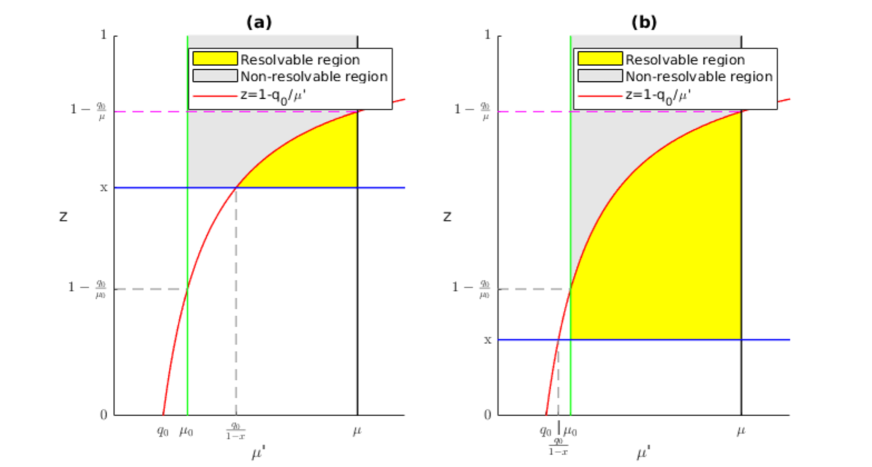
Figure 2: The angular ordering condition $z_{M}(\mu^{\prime})=1-q_{0}/\mu^{\prime}$ with the resolvable and non-resolvable emission regions in the $(\mu^{\prime},z)$ plane: a) the case $1>x\geq 1-q_{0}/\mu_{0}$; b) the case $1-q_{0}/\mu_{0}>x>0$.

Given the minimum transverse momentum $q_{0}$ and the lowest scale $\mu_{0}$ of the branching, for any $x$ it is useful to distinguish the two cases illustrated in Fig. 2, depending on whether a) $\mu_{0}\leq q_{0}/(1-x)$ or b) $\mu_{0}>q_{0}/(1-x)$. For any $z$ with $x\leq z\leq 1$, in case a) the emitted transverse momentum spans the interval $q_{0}\leq q_{\perp}\leq\mu(1-z)$, while in case b) we have $\mu_{0}(1-z)\leq q_{\perp}\leq\mu(1-z)$. This results into different forms of the branching equations in the two cases, once they are expressed directly in terms of transverse momenta.

3.1 Case a) $1>x\geq 1-{q_{0}}/{\mu_{0}}$

For $x\geq 1-{q_{0}}/{\mu_{0}}$ the resolvable emission region is mapped to the domain in the $(z,q_{\bot})$ plane pictured in Fig. 3(a). We change integration variable from $\mu^{\prime}$ to $q_{\perp}$ in the branching equation (10) using the angular ordering relation (4). Then Eq. (10) can be recast in terms of transverse momenta as

$$\widetilde{f}_{a}(x,\mu^{2}) = \Delta_{a}(\mu^{2},\mu_{0}^{2})\widetilde{f}_{a}(x,\mu_{0}^{2})+\sum_{b}\int\frac{\textrm{d}q_{\bot}^{2}}{q_{\bot}^{2}}\int_{x}^{1}\textrm{d}z\ \Theta(q_{\perp}^{2}-q_{0}^{2})\ \Theta(\mu^{2}(1-x)^{2}-q_{\perp}^{2})$$ (11)

$$\times \Theta(1-q_{\perp}/\mu-z)\ \frac{\Delta_{a}(\mu^{2},\mu_{0}^{2})}{\Delta_{a}\left(q_{\bot}^{2}/(1-z)^{2},\mu_{0}^{2}\right)}\ P^{R}_{ab}\left(z,\alpha_{s}\left(q_{\bot}^{2}\right)\right)\widetilde{f}_{b}\left(\frac{x}{z},\frac{q_{\bot}^{2}}{(1-z)^{2}}\right)\;.$$

3.2 Case b) $1-{q_{0}}/{\mu_{0}}>x>0$

For $x<1-{q_{0}}/{\mu_{0}}$ the resolvable emission region is mapped to the domain in the $(z,q_{\bot})$ plane pictured in Fig. 3(b). Performing the same change of integration variable in Eq. (10) as in case a) of the previous subsection, we recognize that now a subtraction term arises from the low-$q_{\perp}$ region, $q_{0}<q_{\perp}<(1-x)\mu_{0}$, so that Eq. (10) is rewritten in terms of transverse momenta as

$$\widetilde{f}_{a}(x,\mu^{2}) = \Delta_{a}(\mu^{2},\mu_{0}^{2})\widetilde{f}_{a}(x,\mu_{0}^{2})+\sum_{b}\int\frac{\textrm{d}q_{\bot}^{2}}{q_{\bot}^{2}}\int_{x}^{1}\textrm{d}z\ \Big{[}\Theta(q_{\perp}^{2}-q_{0}^{2})\ \Theta(\mu^{2}(1-x)^{2}-q_{\perp}^{2})$$ (12)

$$\times \Theta(1-q_{\perp}/\mu-z)-\Theta(q_{\perp}^{2}-q_{0}^{2})\ \Theta(\mu_{0}^{2}(1-x)^{2}-q_{\perp}^{2})\ \Theta(1-q_{\perp}/\mu_{0}-z)\Big{]}$$

$$\times \frac{\Delta_{a}(\mu^{2},\mu_{0}^{2})}{\Delta_{a}\left(q_{\bot}^{2}/(1-z)^{2},\mu_{0}^{2}\right)}\ P^{R}_{ab}\left(z,\alpha_{s}\left(q_{\bot}^{2}\right)\right)\widetilde{f}_{b}\left(\frac{x}{z},\frac{q_{\bot}^{2}}{(1-z)^{2}}\right)\;.$$

We observe that the first term in the square bracket in Eq. (12) is a contribution analogous to that in Eq. (11), while the second term in the square bracket provides the low-$q_{\perp}$ subtraction.

Alternatively, the branching kernel in the case $x<1-{q_{0}}/{\mu_{0}}$ can be expressed as a sum of two contributions, corresponding respectively to the $q_{\perp}<(1-x)\mu_{0}$ region and $q_{\perp}>(1-x)\mu_{0}$ region, as follows

$$\widetilde{f}_{a}(x,\mu^{2}) = \Delta_{a}(\mu^{2},\mu_{0}^{2})\widetilde{f}_{a}(x,\mu_{0}^{2})+\sum_{b}\int\frac{\textrm{d}q_{\bot}^{2}}{q_{\bot}^{2}}\int_{x}^{1}\textrm{d}z\Big{[}\Theta(q_{\perp}^{2}-q_{0}^{2})\Theta(\mu_{0}^{2}(1-x)^{2}-q_{\perp}^{2})$$ (13)

$$\times \Theta(z+q_{\perp}/\mu_{0}-1)\Theta(1-q_{\perp}/\mu-z)+\Theta(q_{\perp}^{2}-(1-x)^{2}\mu_{0}^{2})\Theta(\mu^{2}(1-x)^{2}-q_{\perp}^{2})$$

$$\times \Theta(1-q_{\perp}/\mu-z)\Big{]}\frac{\Delta_{a}(\mu^{2},\mu_{0}^{2})}{\Delta_{a}\left(q_{\bot}^{2}/(1-z)^{2},\mu_{0}^{2}\right)}P^{R}_{ab}\left(z,\alpha_{s}\left(q_{\bot}^{2}\right)\right)\widetilde{f}_{b}\left(\frac{x}{z},\frac{q_{\bot}^{2}}{(1-z)^{2}}\right)\;.$$

Here the two terms of the sum in the square bracket, given by products of $\Theta$ functions, describe the low-$q_{\perp}$ and high-$q_{\perp}$ contributions.

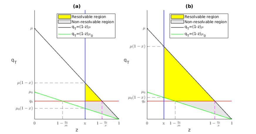
Figure 3: Resolvable and non-resolvable emission regions in the $(z,q_{\bot})$ plane for evolution in the cases a) $1>x\geq 1-q_{0}/\mu_{0}$ and b) $1-q_{0}/\mu_{0}>x>0$.

In the next section we will use the form for the branching equations derived above, along with the formulas of Sec. 2, to carry out a comparison of the PB method [3, 4] with other existing approaches in the literature. We will analyze in particular different treatments of the QCD parton cascade, in which the transverse momentum is generated either through multiple emissions or through a single emission.

4 Multiple-emission versus single-emission approaches

As an approach based on the unitarity picture [5, 6] of parton evolution and angular ordering, the PB method [3, 4] can naturally be compared with the coherent branching approach [9, 10] of Catani-Marchesini-Webber (CMW). Since Refs. [9, 10] do not construct TMD distributions, we examine branching equations in the PB and CMW approaches at the level of integrated distributions. At this level, we observe that Eq. (10) agrees with the CMW result — see Eqs. (42), (49) and Sec. 3.4 of [9]. In Ref. [9] this branching equation is studied at LO with one-loop splitting kernels and running coupling, while in Ref. [3] (and in the present paper) it is studied at NLO with two-loop splitting kernels and running coupling.

The Kimber-Martin-Ryskin-Watt (KMRW) approach [13, 14, 15, 16], on the other hand, is designed to construct TMD unintegrated distributions. In contrast to the PB method, in which the transverse momentum and the branching scale are calculated at each branching as illustrated in Fig. 1, KMRW is a one-step evolution approach: it performs evolution in one scale up to $q_{\bot}^{2}$, while the second scale is generated only in the last step of the evolution. The KMRW physical picture is thus quite different from that of PB and CMW. In particular, in KMRW the transverse momentum is produced as a result of a single emission, while in PB it is built from multiple emissions.

We next perform comparisons of KMRW and PB distributions. In the KMRW literature, the distinction between the values of the two momentum scales $\mu_{0}$ and $q_{0}$ discussed in Sec. 3 is not made. For the purpose of this comparison, therefore, we set $q_{0}\approx\mu_{0}$ in the formulation of Sec. 3, and we will thus be using the branching equation valid in case a) of Subsec. 3.1, Eq. (11).

4.1 Comparison with the KMRW approach

In the KMRW approach the TMD distribution is written as [13, 14, 15, 16]

$$\widetilde{D}_{a}(x,\mu^{2},q_{\bot}^{2}) = T_{a}(\mu^{2},q_{\bot}^{2})\sum_{b}\int_{x}^{1-C(q_{\bot},\mu)}dzP^{R}_{ab}\left(z,\alpha_{s}(q_{\bot}^{2})\right)\widetilde{f}_{b}\left(\frac{x}{z},q_{\bot}^{2}\right)\;\;,$$ (14)

where the Sudakov form factor is given by

$$T_{a}(\mu^{2},q_{\bot}^{2})=\exp\left[-\int_{q_{\bot}^{2}}^{\mu^{2}}\frac{\textrm{d}q_{\bot}^{\prime 2}}{q_{\bot}^{\prime 2}}\sum_{b}\int_{0}^{1-C(q_{\bot}^{\prime},\mu)}\textrm{d}zzP_{ba}^{R}\left(z,\alpha_{s}\left(q_{\bot}^{\prime 2}\right)\right)\right]\;,$$ (15)

and the collinear density $\widetilde{f}_{a}(x,\mu^{2})$ obeys the evolution equation

$$\widetilde{f}_{a}(x,\mu^{2}) = \widetilde{f}_{a}(x,\mu_{0}^{2})T_{a}(\mu^{2},\mu_{0}^{2})$$ (16)

$$+ \int_{\mu_{0}^{2}}^{q_{\bot M}^{2}}\frac{dq_{\bot}^{2}}{q_{\bot}^{2}}\left(T_{a}(\mu^{2},q_{\bot}^{2})\sum_{b}\int_{x}^{1-C(q_{\bot},\mu)}dzP^{R}_{ab}\left(z,\alpha_{s}(q_{\bot}^{2})\right)\widetilde{f}_{b}\left(\frac{x}{z},q_{\bot}^{2}\right)\right)\;.$$

The phase space parameters $C(q_{\bot},\mu)$ and $q_{\bot M}$ in the above formulas are assigned according to two distinct prescriptions [13, 14, 15, 16, 26] in the KMRW approach:

$$C(q_{\bot},\mu)={q_{\bot}}/{\mu}\;\;,\;\;\;\;q_{\bot M}=\mu(1-x)\;\;\;\;{\rm{for}}\;\;{\rm{KMRW}}\;\;{\rm{strong}}\;\;{\rm{ordering}}$$ (17)

and

$$C(q_{\bot},\mu)={q_{\bot}}/({q_{\bot}+\mu})\;\;,\;\;\;\;q_{\bot M}=\mu({1-x})/{x}\;\;\;{\rm{for}}\;\;{\rm{KMRW}}\;\;{\rm{angular}}\;\;{\rm{ordering}}.$$ (18)

Having mapped the PB evolution onto transverse momenta in Sec. 3, we are in a position to directly compare the PB and KMRW results. By considering Eq. (11) and Eq. (16) with KMRW strong ordering conditions (17), we recognize that PB and KMRW differ in the momentum scales at which both the Sudakov form factor and the collinear density $\widetilde{f}_{b}$ are evaluated, as KMRW uses transverse momenta whereas PB uses transverse momenta rescaled by $1/(1-z)$. From Eq. (11) and Eq. (16) with KMRW angular ordering conditions (18), we recognize that in this case PB and KMRW, besides differing in the arguments of Sudakov factor and collinear density, differ also in the phase space regions in longitudinal and transverse momenta that are populated by the radiative processes.

We thus see that, also taking into account the possible prescriptions in Eqs. (17) and (18), the one-step picture of KMRW leads to different results from the multiple-emission PB picture. In Sec. 5 we illustrate the implications of these differences by performing numerical calculations for the TMD distributions that result from evolution in the two approaches, and examining the corresponding predictions for the DY $Z$-boson transverse momentum spectra at the LHC.

4.2 Remark on Sudakov form factors

It is worth noting that the definition of the Sudakov form factor itself plays a different role in the context of the PB approach and the KMRW approach.

In the PB approach the Sudakov form factor $\Delta_{a}(\mu^{2},\mu_{0}^{2})$ has the interpretation of probability for no resolvable branching in a given evolution interval from $\mu_{0}$ to $\mu$, and fulfills the property

$$\Delta_{a}(\mu^{2},\widetilde{\mu}^{2})\Delta_{a}(\widetilde{\mu}^{2},\mu_{0}^{2})=\Delta_{a}(\mu^{2},\mu_{0}^{2})\;$$ (19)

for any evolution scale $\widetilde{\mu}$.

For example, for the Sudakov form factor in the angular-ordered evolution we use

$$\Delta_{a}(\mu^{2},\mu_{0}^{2})=\exp\left(-\sum_{b}\int_{\mu_{0}^{2}}^{\mu^{2}}\frac{\textrm{d}\mu^{\prime 2}}{\mu^{\prime 2}}\int_{0}^{1-{q_{0}}/{\mu^{\prime}}}\textrm{d}z\ z\ P^{R}_{ba}\left(z,\alpha_{s}\left((1-z)^{2}\mu^{\prime 2}\right)\right)\right)\;,$$ (20)

for which Eq. (19) is fulfilled. Upon mapping to transverse momenta, this becomes

$$\Delta_{a}(\mu^{2},\mu_{0}^{2})=\exp\left[-\sum_{b}\left(\int_{\mu_{0}^{2}}^{\mu^{2}}\frac{\textrm{d}q_{\bot}^{2}}{q_{\bot}^{2}}\int_{0}^{1-{q_{\bot}}/{\mu}}\textrm{d}z+\int_{q_{0}^{2}}^{\mu_{0}^{2}}\frac{\textrm{d}q_{\bot}^{2}}{q_{\bot}^{2}}\int_{1-{q_{\bot}}/{\mu_{0}}}^{1-{q_{\bot}}/{\mu}}\textrm{d}z\right)z\ P_{ba}^{R}\left(z,\alpha_{s}\left(q_{\bot}^{2}\right)\right)\right]\;,$$ (21)

for which Eq. (19) is still fulfilled.

On the other hand, using the KMRW expression in Eq. (15), Eq. (19) is not fulfilled. Rather, one has

$$T_{a}(\mu^{2},k_{\bot}^{2})T_{a}(k_{\bot}^{2},\mu_{0}^{2})=T_{a}(\mu^{2},\mu_{0}^{2})\exp\left(\sum_{b}\int_{\mu_{0}^{2}}^{k_{\bot}^{2}}\frac{\textrm{d}q_{\bot}^{2}}{q_{\bot}^{2}}\int_{1-C(q_{\bot},k_{\bot})}^{1-C(q_{\bot},\mu)}\textrm{d}z\ z\ P_{ba}^{R}(z,\alpha_{s}(q_{\bot}^{2}))\right)\;.$$ (22)

This implies that, besides the different treatment of radiative processes noted in Subsec. 4.1, we observe differences between the single-emission and multiple-emission approaches also in the treatment of the non-resolvable processes. We may expect that the features noted in Subsec. 4.1 and in this subsection will lead to different behaviors in transverse momentum distributions both at high transverse momenta and at low transverse momenta.

5 Numerical results

We investigate next the numerical implications of the analysis in the previous sections on TMD distributions and DY spectra.

5.1 TMDs from PB and KMRW

In this section we present numerical results for TMD distribution functions from the PB approach with dynamical resolution scale. We perform numerical comparisons with KMRW TMDs. The results are shown as functions of flavor, longitudinal momentum fraction $x$, transverse momentum $k_{\perp}$, evolution scale $\mu$.

KMRW TMD distribution sets have been obtained in [27] according to the KMRW angular ordering prescription (18), using the CT10nlo PDF [28] set as a starting collinear distribution and a flat parameterization for $k_{\bot}<1\;\textrm{GeV}$ as an intrinsic $k_{\bot}$ distribution at starting scale $\mu_{0}$. These distributions have been included in the TMDlib library [29] under the name MRW-CT10nlo.

To evaluate PB TMDs, we solve numerically Eq. (1), with the angular ordering condition in Eq. (4), the dynamical resolution scale in Eq. (8) where we take $q_{0}=1\;\textrm{GeV}$, and the scale of $\alpha_{s}$ in Eq. (6). We use the Monte Carlo solution method developed in [3, 4] and implemented in the package uPDFevolv [12]. Following [18], we take intrinsic $k_{\bot}$ distribution given by a simple gaussian at starting scale $\mu_{0}$ with (flavor-independent and $x$-independent) width $\sigma=k_{0}/\sqrt{2}$, $k_{0}=0.5$ GeV. For the purpose of performing comparisons with the KMRW TMD set MRW-CT10nlo, we take the same starting collinear distribution CT10nlo [28]. We also note that the infrared region with the Landau pole of the coupling in Eq. (6) is avoided by using the dynamical resolution scale (8) with $q_{0}=1\;\textrm{GeV}$.

In addition, we introduce an approximation to the PB framework, which we refer to as “PB-last-step”, which is obtained from PB by taking the same settings as the full PB calculation but restricting the transverse momentum $k_{\bot}$ to the last emission only. We use the PB-last-step Monte Carlo simulation as a guidance to distinguish effects from single emission and multiple emissions.

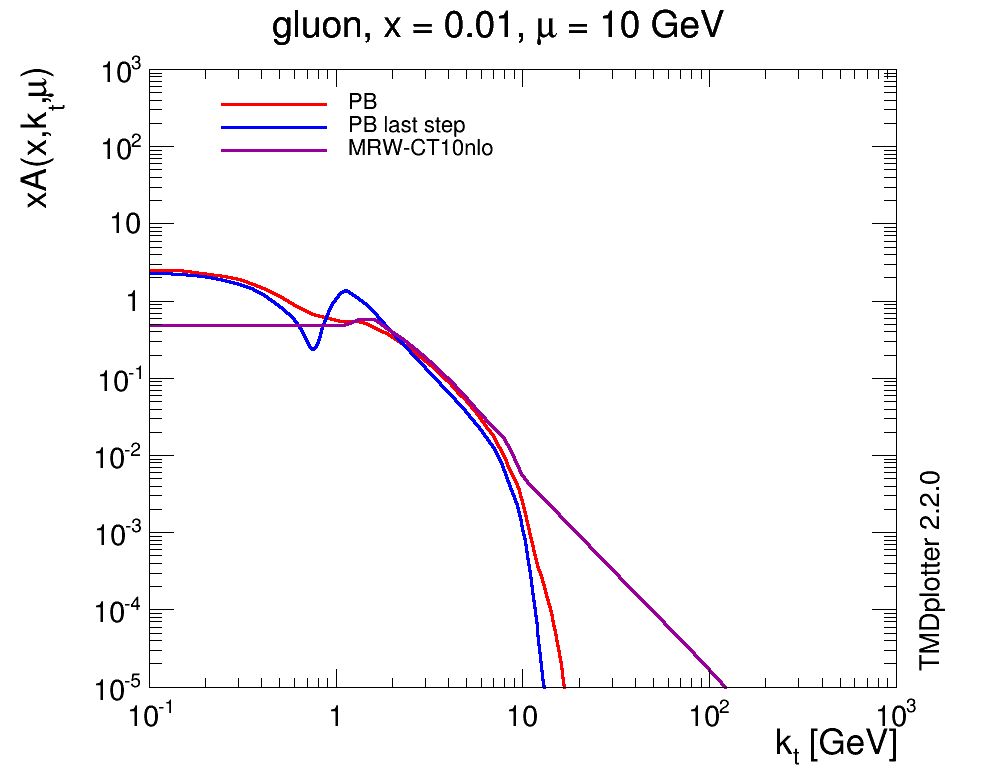
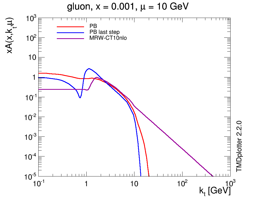
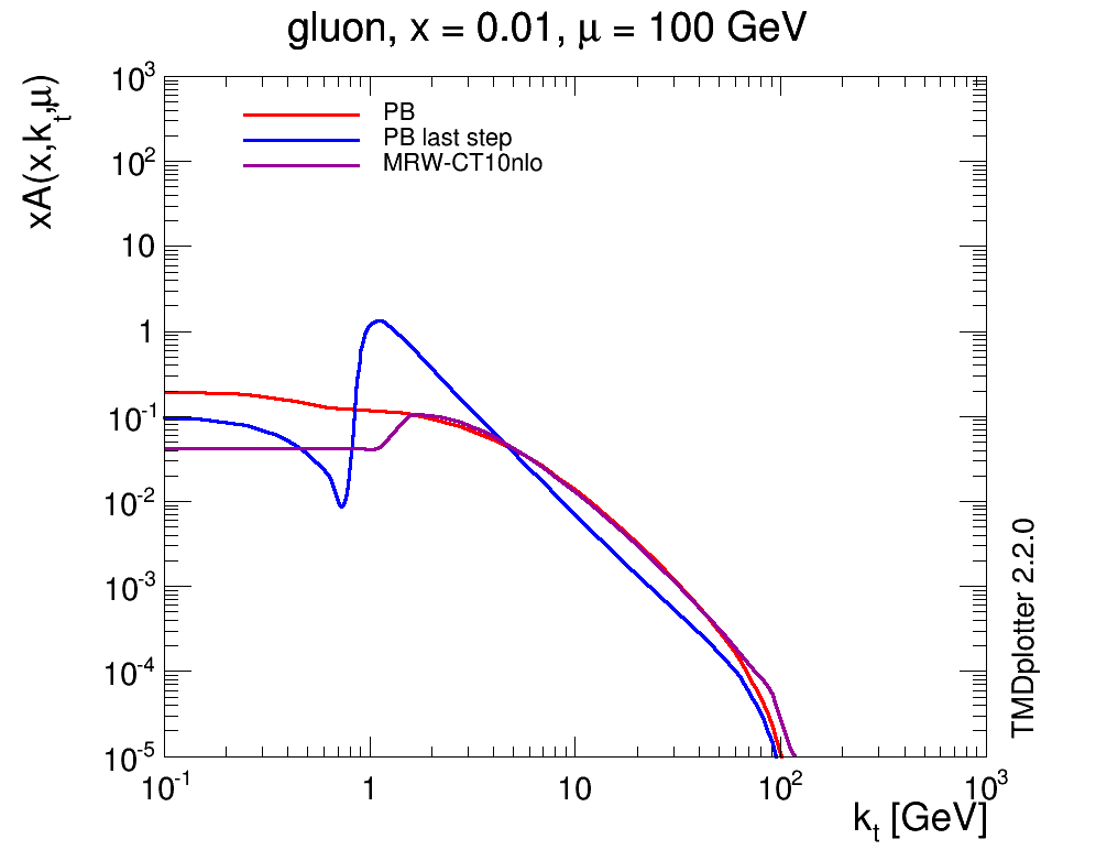
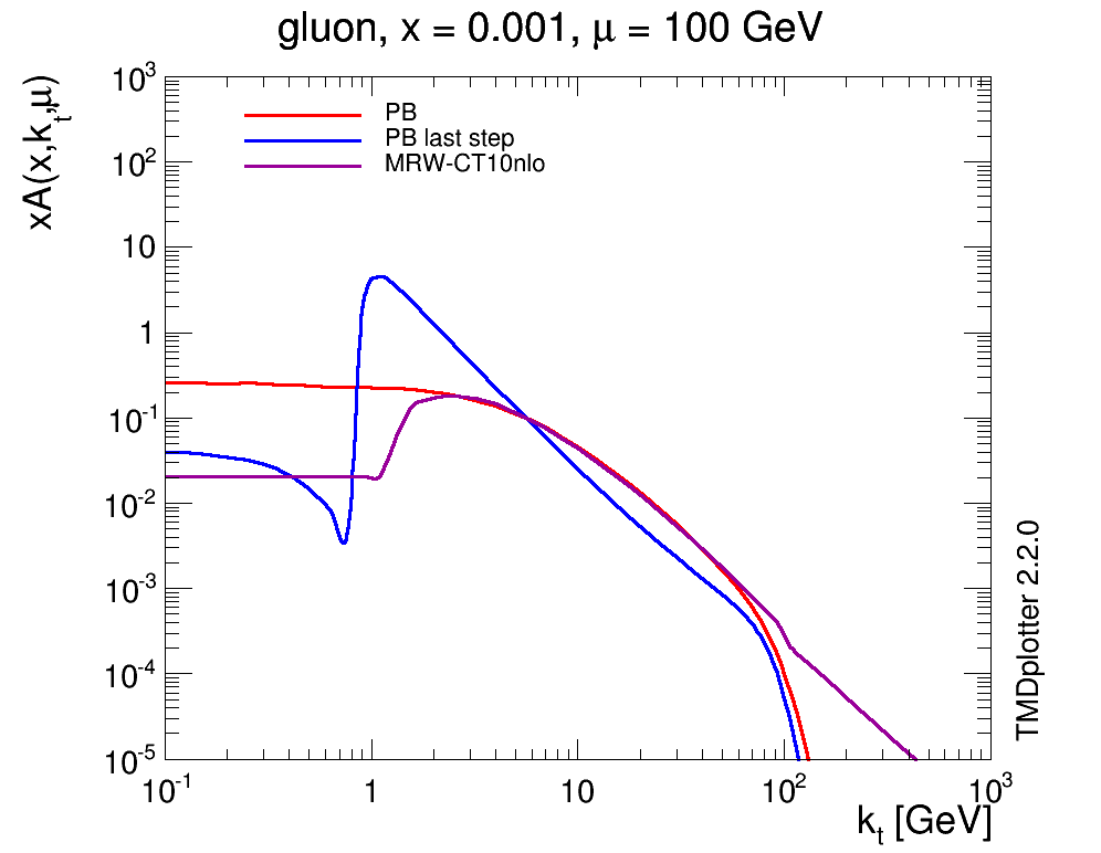
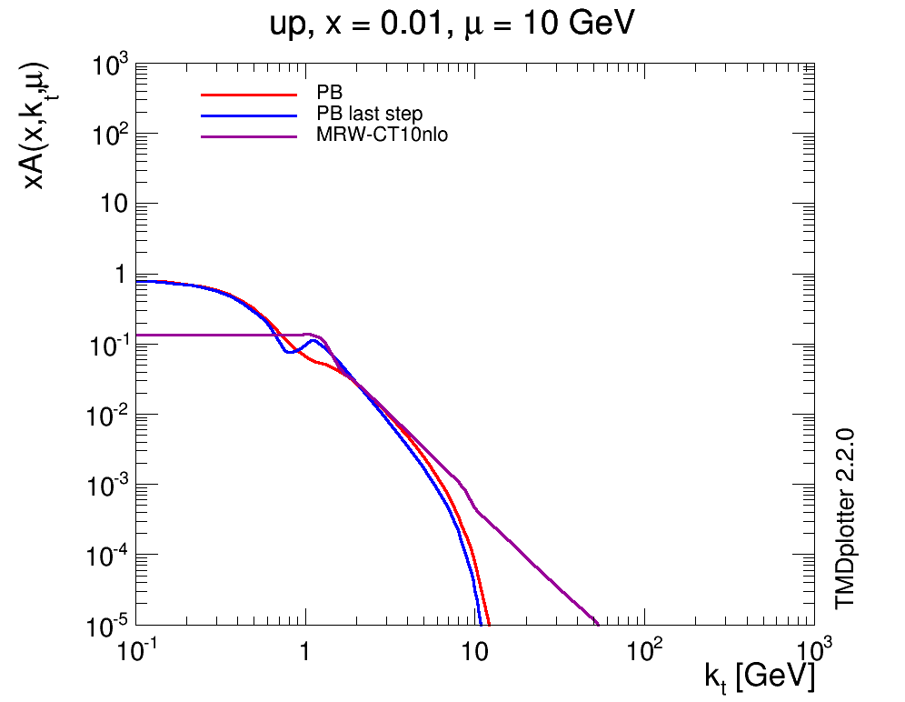
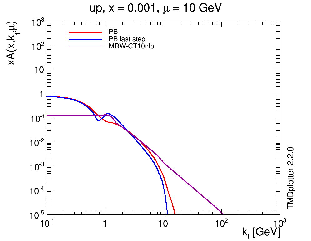
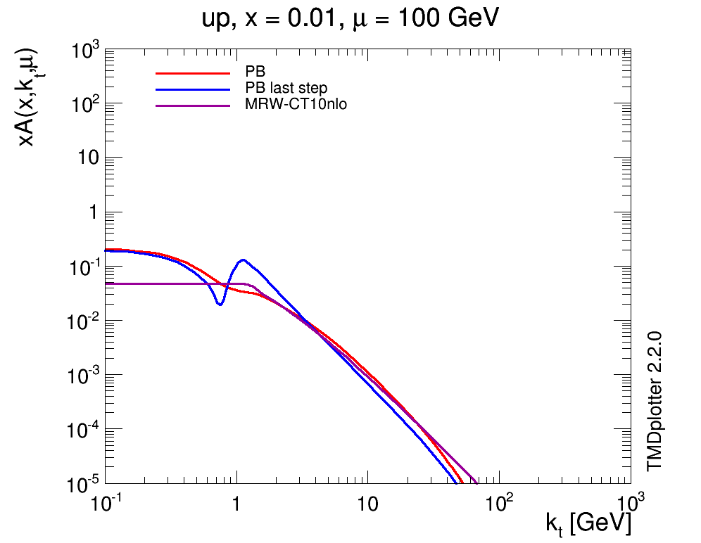
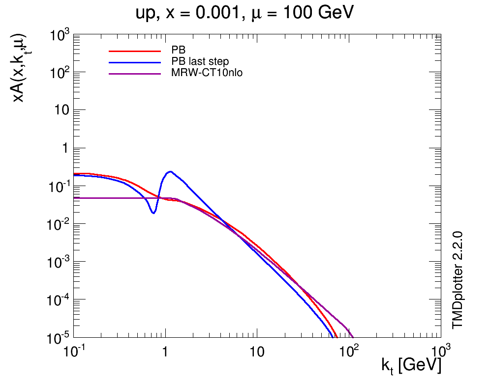
Figure 4: TMDs from PB and KMRW as functions of transverse momentum for different parton species and different values of longitudinal momentum fraction $x$ and evolution scale $\mu$.

In Fig. 4 we show results for the $k_{\bot}$ dependence from PB, MRW-CT10nlo and PB-last-step calculations, at different values of $x$ and $\mu$. We may distinguish three regions of low $k_{\bot}$, middle $k_{\bot}$ and high $k_{\bot}$, characterized by distinct behaviors. Significant numerical differences between PB and KMRW show up especially in the extreme regions $k_{\bot}\ll\mu$ and $k_{\bot}\gg\mu$, while in an interval of middle values around $k_{\bot}\sim\mu$ the two predictions tend to become closer.

In particular, we observe that at low $k_{\bot}$ the smearing of the intrinsic $k_{\bot}$ distribution due to evolution gives rise to different behaviors in the single-emission and multiple-emission cases. The kink at low $k_{\bot}$ in MRW-CT10nlo is a consequence of the single-emission picture, and is not present in the full PB case, where multiple branchings are responsible for generating the transverse momentum.

We also observe that at high $k_{\bot}$ the MRW-CT10nlo distribution is far harder than PB and PB-last-step. This reflects the different pattern of radiative contributions in KMRW from PB, illustrated in Sec. 4. As noted in [27], the treatment of the Sudakov form factor for $k_{\bot}^{2}>\mu^{2}$ influences the MRW-CT10nlo high $k_{\bot}$ tail.

On the other hand, notice that MRW-ct10nlo and PB are closer in the middle range of $k_{\bot}$ comparable to the scale $\mu$. In this range, the differences between KMRW and PB approaches in the parton-density and Sudakov-factor rescaling and phase space, discussed in the previous section, compensate for KMRW not taking into account all previous emissions compared to PB. The net effect is that the behaviors of KMRW and PB are not too dissimilar for mid $k_{\bot}$.

Results for the $x$ dependence from PB, MRW-CT10nlo and PB-last-step calculations are shown in Fig. 5, illustrating that the effects noted above persist over a broad range in $x$.

In Fig. 6 the results of integrating MRW-CT10nlo, PB and PB-last-step TMDs over the transverse momentum $k_{\bot}$ at a given evolution scale $\mu$ are shown as functions of $x$. Results are shown for integrating TMDs over $k_{\bot}<\mu$ (Fig. 6(left)) and over all $k_{\bot}$ (Fig. 6(right)). For comparison, we also plot CT10nlo distributions at the same $\mu$. In the lower parts of the figure the ratios of integrated TMDs to CT10nlo are plotted. As expected, we observe that none of the distributions integrate to CT10nlo, given that the resolution scale $z_{M}$ is far from 1, and the scale of the running coupling $\alpha_{s}$ is $q_{\bot}$ — see remarks below Eq. (9). In the case of integrating over all $k_{\bot}$ (Fig. 6(right)) we note that MRW-CT10nlo gives rise to a much higher distribution than all other curves, implying that the MRW-CT10nlo high-$k_{\bot}$ tail has a significant impact at integrated level for most values of $x$. On the other hand, when integrating over $k_{\bot}<\mu$ (Fig. 6(left)) the deviation of MRW-CT10nlo from collinear CT10nlo is smaller than that of PB, which is a further manifestation of the differences between the KMRW and PB physical pictures illustrated in Sec. 4.

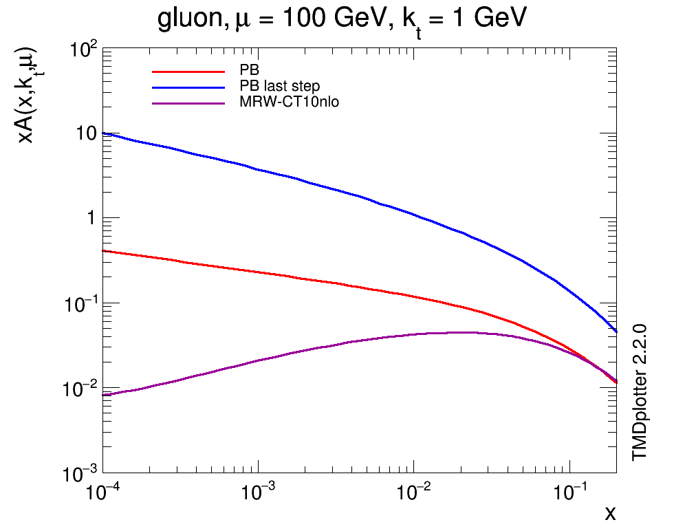
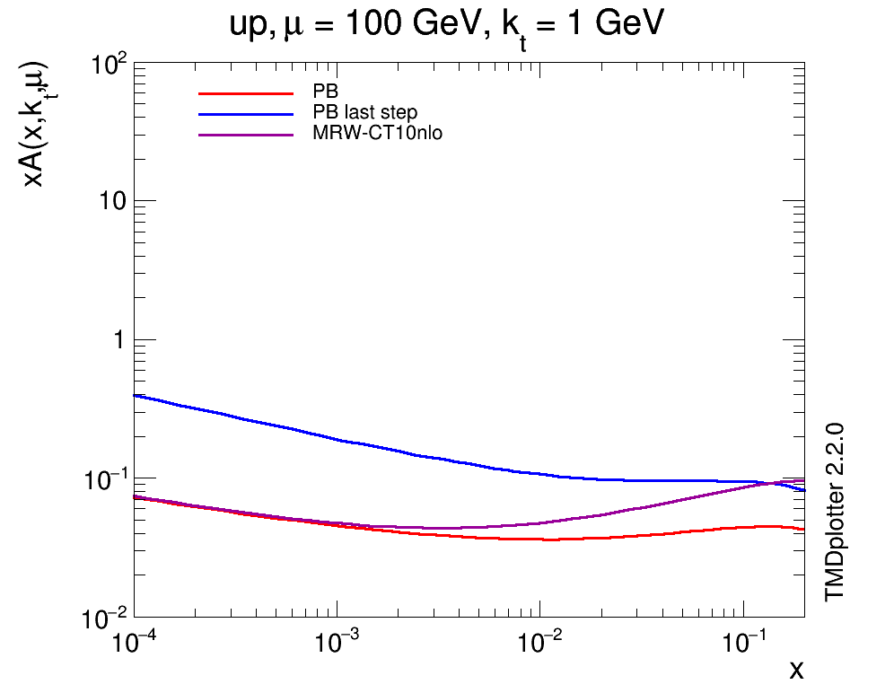
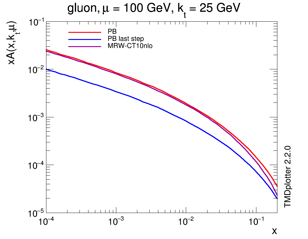
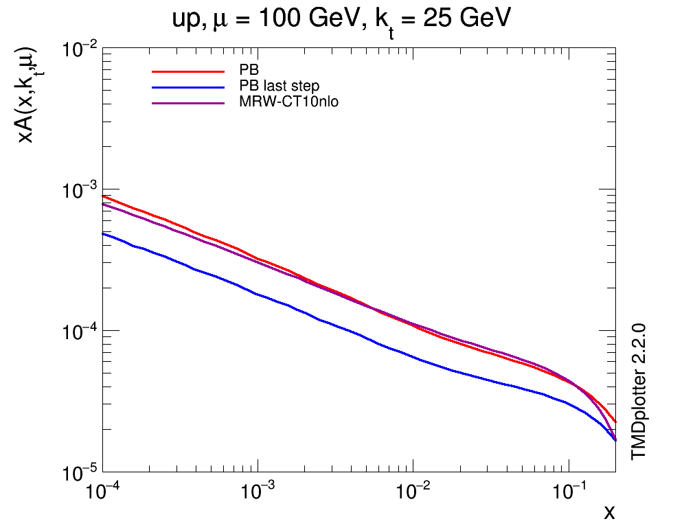
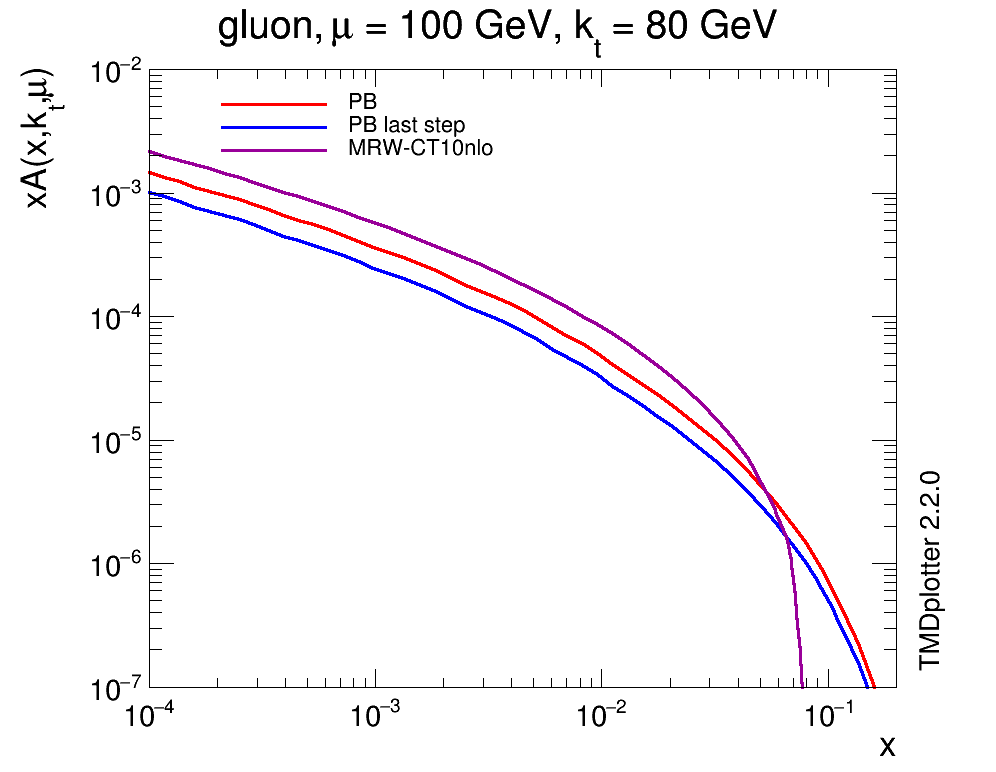
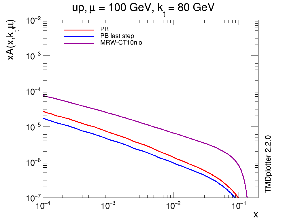
Figure 5: TMDs from PB and KMRW as functions of $x$.

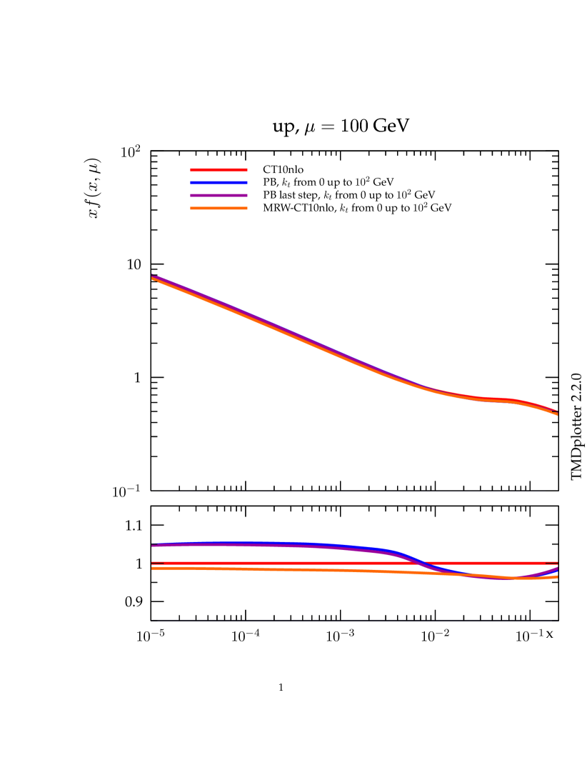
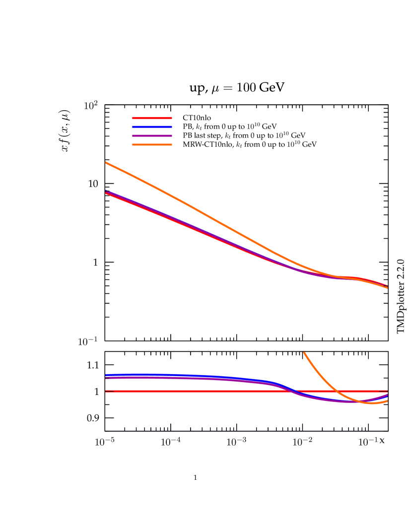
Figure 6: The results of integrating TMDs over $k_{\bot}<\mu$ (left) and over all $k_{\bot}$ (right) as functions of $x$.

5.2 DY $Z$-boson $p_{\bot}$ spectrum

$Z$-boson transverse momentum spectra in DY di-lepton production have been measured with high precision at the LHC [31, 32, 33, 34]. In the region of transverse momenta $p_{\bot}$ small compared to the di-lepton invariant mass, the spectrum is sensitive to Sudakov resummation. Reliable theoretical predictions require soft-gluon resummations and nonperturbative contributions, which can be included by using the TMD theoretical framework. We here follow the treatment [18] to apply PB TMDs to the DY $p_{\bot}$ spectrum. We obtain predictions for the $Z$-boson distribution based on PB TMDs that include effects of dynamical soft-gluon resolution scale. We compare them with KMRW results. We perform a comparison of theoretical results with the LHC measurements [31].

Following [18], as we are interested mainly in the low $p_{\bot}$ region of the DY spectrum we use on-shell LO matrix elements (in the format of Les Houches Event (LHE) file [35]) generated by Pythia Monte Carlo [36]. The transverse momentum of the initial state partons is calculated according to the TMDs and added to the event record in such a way that the mass of the produced DY pair is conserved, while the longitudinal momenta are changed accordingly. This procedure is common in standard parton shower approaches [37, 38] and is implemented in the Cascade package [39]. Events in HEPMC [40] format are produced and analyzed with Rivet [41].

In Fig. 7 predictions for the Z boson $p_{\bot}$ spectrum at the LHC with $\sqrt{s}=8\;\textrm{TeV}$ are shown using MRW-CT10nlo and PB TMDs, and compared to the ATLAS measurements [31]. For reference, we also plot PB results for fixed (non-dynamical) resolution scale $z_{M}$ using the PB TMD Set-2 of Ref. [18]. We see that the MRW-CT10nlo calculation and PB calculation with dynamical $z_{M}$ give rise to different shapes in the $Z$-boson $p_{\bot}$ spectrum both in the region of low $p_{\bot}$ around the peak and in the region of high $p_{\bot}$ toward the upper end of the transverse momentum range shown. There is an interval of intermediate $p_{\bot}$ in which they are less dissimilar. The agreement of the PB calculation with the measurements is good, while MRW-CT10nlo does not describe the high $p_{\bot}$ region, and the slope at low $p_{\bot}$.

Fig. 7 also illustrates the effect of the soft-gluon dynamical resolution scale by comparing PB predictions with fixed and dynamical $z_{M}$. We see that the slope of the $p_{\bot}$ spectrum is affected by dynamical $z_{M}$ particularly in the low $p_{\bot}$ region. The results indicate that measurements of the $Z$ boson $p_{\bot}$ with high resolution in the region $p_{\perp}\raisebox{-2.58334pt}{\hbox to0.0pt{$\,\sim\,$\hss}}\raisebox{1.72218pt}{$\,<\,$}$ 5 - 10 GeV will allow one to probe quantitatively effects of soft-gluon angular ordering and dynamical resolution scales. This will also be relevant to investigate effects from transverse momentum dependence in the branching probabilities (see e.g. [42, 43]).

We have limited ourselves to showing results for central values of the predictions, because TMD uncertainties in the case of dynamical $z_{M}$ are not yet available. The results obtained provide a strong motivation for extending the PB TMD fits and determination of TMD uncertainties [18] to include dynamical resolution scales. We leave this to future work.

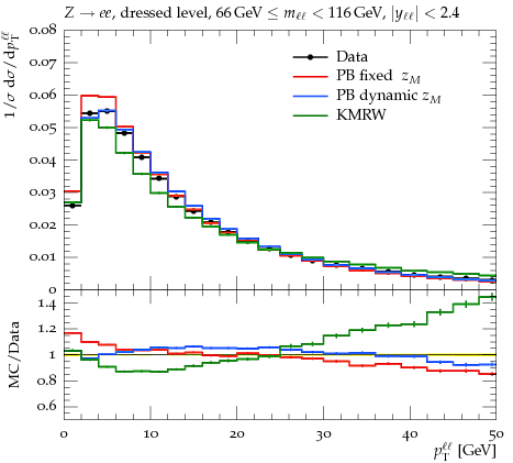
Figure 7: Predictions for the $Z$-boson $p_{\bot}$ spectrum obtained with PB and MRW-CT10nlo TMDs compared to the $8\;\textrm{TeV}$ ATLAS measurement [31].

6 Conclusions

In this paper, using the PB method [3, 4] for angular-ordered TMD evolution, we have studied physical implications of the dependence of the soft-gluon resolution parameter on the branching scale. Mapping the phase space of resolvable and non-resolvable emissions from $(\mu^{\prime},z)$ space to $(z,q_{\bot})$ space, we have written down the corresponding form of the evolution kernel. We have established the comparison of the PB formulation with other existing formulations, notably the ones known as CMW [9, 10] and KMRW [13, 14, 15, 16].

On one hand, we find that the PB formula coincides with CMW at the level of integrated distributions. CMW was originally developed by evaluating splitting kernels at LO, while we evaluate the kernels at NLO. On the other hand, we find significant differences of PB with respect to KMRW, which can be traced back to the fact that PB builds the initial-state transverse momentum from multiple emissions, while KMRW builds it from single emission — the last step in the initial-state evolution cascade. We examine these differences in detail both analytically and numerically. We find that the numerical effects are large in the extreme regions of low $k_{\perp}$ and high $k_{\perp}$, but small in the middle $k_{\perp}$ region.

We apply the results to the evaluation of the DY $Z$-boson $p_{\perp}$ spectrum and comparison with LHC measurements. We compare PB versus KMRW, finding significantly different behaviors in the low-$p_{\perp}$ and high-$p_{\perp}$ regions. We study the sensitivity of the $Z$-boson spectrum to effects of the soft-gluon resolution scale, and observe that these could be accessed by detailed measurements of the $Z$-boson transverse momentum with fine binning in the region $p_{\perp}\raisebox{-2.58334pt}{\hbox to0.0pt{$\,\sim\,$\hss}}\raisebox{1.72218pt}{$\,<\,$}$ 5 - 10 GeV.

Acknowledgments. We thank M. Bury for helpful correspondence on the MRW-CT10nlo implementation, and K. Golec-Biernat, H. Jung and S. Plätzer for useful discussions. We gratefully acknowledge the hospitality and support of the Erwin Schrödinger Institute at the University of Vienna and Nuclear Physics Institute of the Polish Academy of Sciences in Krakow while part of this work was being done.

References

- [1] G. Luisoni and S. Marzani, J. Phys. G42, 103101 (2015). 1505.04084
- [2] R. Angeles-Martinez et al., Acta Phys. Polon. B46, 2501 (2015). 1507.05267
- [3] F. Hautmann, H. Jung, A. Lelek, V. Radescu, and R. Zlebcik, Phys. Lett. B772, 446 (2017). 1704.01757
- [4] F. Hautmann, H. Jung, A. Lelek, V. Radescu, and R. Zlebcik, JHEP 01, 070 (2018). 1708.03279
- [5] B. R. Webber, Ann. Rev. Nucl. Part. Sci. 36, 253 (1986)
- [6] R.K.Ellis, W.J.Stirling, and B. Webber, QCD and Collider Physics. Cambridge University Press, 2003
- [7] A. Bassetto, M. Ciafaloni, and G. Marchesini, Phys. Rept. 100, 201 (1983)
- [8] Y. L. Dokshitzer, V. A. Khoze, S. I. Troian, and A. H. Mueller, Rev. Mod. Phys. 60, 373 (1988)
- [9] G. Marchesini and B. R. Webber, Nucl. Phys. B310, 461 (1988)
- [10] S. Catani, B. R. Webber, and G. Marchesini, Nucl. Phys. B349, 635 (1991)
- [11] F. Hautmann, Phys. Lett. B655, 26 (2007). hep-ph/0702196
- [12] F. Hautmann, H. Jung, and S. T. Monfared, Eur. Phys. J. C74, 3082 (2014). 1407.5935
- [13] M. A. Kimber, A. D. Martin, and M. G. Ryskin, Eur. Phys. J. C12, 655 (2000). hep-ph/9911379
- [14] M. A. Kimber, A. D. Martin, and M. G. Ryskin, Phys. Rev. D63, 114027 (2001). hep-ph/0101348
- [15] G. Watt, A. D. Martin, and M. G. Ryskin, Eur. Phys. J. C31, 73 (2003). hep-ph/0306169
- [16] A. D. Martin, M. G. Ryskin, and G. Watt, Eur. Phys. J. C66, 163 (2010). 0909.5529
- [17] S. D. Drell and T.-M. Yan, Phys. Rev. Lett. 25, 316 (1970). [Erratum: Phys. Rev. Lett.25,902(1970)]
- [18] A. Bermudez Martinez, P. Connor, H. Jung, A. Lelek, R. Zlebcik, F. Hautmann, and V. Radescu, Phys. Rev. D99, 074008 (2019). 1804.11152
- [19] A. Bermudez Martinez et al. (2019). 1906.00919
- [20] F. Hautmann, TMDs and Monte Carlo Event Generators, in 23rd International Symposium on Spin Physics (SPIN 2018) Ferrara, Italy, September 10-14, 2018. 2019. Also in preprint 1907.03353
- [21] V. N. Gribov and L. N. Lipatov, Sov. J. Nucl. Phys. 15, 438 (1972). [Yad. Fiz.15,781(1972)]
- [22] L. N. Lipatov, Sov. J. Nucl. Phys. 20, 94 (1975). [Yad. Fiz.20,181(1974)]
- [23] G. Altarelli and G. Parisi, Nucl. Phys. B126, 298 (1977)
- [24] Y. L. Dokshitzer, Sov. Phys. JETP 46, 641 (1977). [Zh. Eksp. Teor. Fiz.73,1216(1977)]
- [25] M. Botje, Comput. Phys. Commun. 182, 490 (2011). 1005.1481
- [26] K. Golec-Biernat and A. M. Stasto, Phys. Lett. B781, 633 (2018). 1803.06246
- [27] M. Bury, A. van Hameren, H. Jung, K. Kutak, S. Sapeta, and M. Serino, Eur. Phys. J. C78, 137 (2018). 1712.05932
- [28] H.-L. Lai, M. Guzzi, J. Huston, Z. Li, P. M. Nadolsky, J. Pumplin, and C. P. Yuan, Phys. Rev. D82, 074024 (2010). 1007.2241
- [29] F. Hautmann, H. Jung, M. Krämer, P. J. Mulders, E. R. Nocera, T. C. Rogers, and A. Signori, Eur. Phys. J. C74, 3220 (2014). 1408.3015
- [30] P. L. S. Connor, H. Jung, F. Hautmann, and J. Scheller, PoS DIS2016, 039 (2016)
- [31] ATLAS Collaboration, G. Aad et al., Eur. Phys. J. C76, 291 (2016). 1512.02192
- [32] ATLAS Collaboration, G. Aad et al., JHEP 09, 145 (2014). 1406.3660
- [33] CMS Collaboration, V. Khachatryan et al., JHEP 02, 096 (2017). 1606.05864
- [34] CMS Collaboration, S. Chatrchyan et al., Phys. Rev. D85, 032002 (2012). 1110.4973
- [35] J. Alwall et al., Comput. Phys. Commun. 176, 300 (2007). hep-ph/0609017
- [36] T. Sjostrand, S. Mrenna, and P. Z. Skands, Comput. Phys. Commun. 178, 852 (2008). 0710.3820
- [37] T. Sjostrand, S. Ask, J. R. Christiansen, R. Corke, N. Desai, P. Ilten, S. Mrenna, S. Prestel, C. O. Rasmussen, and P. Z. Skands, Comput. Phys. Commun. 191, 159 (2015). 1410.3012
- [38] M. Bengtsson, T. Sjostrand, and M. van Zijl, Z. Phys. C32, 67 (1986)
- [39] H. Jung et al., Eur. Phys. J. C70, 1237 (2010). 1008.0152
- [40] M. Dobbs and J. B. Hansen, Comput. Phys. Commun. 134, 41 (2001)
- [41] A. Buckley, J. Butterworth, L. Lonnblad, D. Grellscheid, H. Hoeth, J. Monk, H. Schulz, and F. Siegert, Comput. Phys. Commun. 184, 2803 (2013). 1003.0694
- [42] F. Hautmann, M. Hentschinski, and H. Jung, Nucl. Phys. B865, 54 (2012). 1205.1759
- [43] F. Hautmann, M. Hentschinski, and H. Jung (2012). 1205.6358.