Experimental Demonstration of Exceptional Points of Degeneracy in Linear Time Periodic Systems and Exceptional Sensitivity

Abstract

We present the experimental demonstration of the occurrence of exceptional points of degeneracy (EPDs) in a single resonator by introducing a linear time-periodic variation of one of its components, in contrast to EPDs in parity time (PT)-symmetric systems that require two coupled resonators with precise values of gain and loss. In the proposed scheme, only the tuning of the modulation frequency is required that is easily achieved in electronic systems. The EPD is a point in a system parameters’ space at which two or more eigenstates coalesce, and this leads to unique properties not occurring at other non-degenerate operating points. We show theoretically and experimentally the existence of a second order EPD in a time-varying single resonator. Furthermore, we measure the sensitivity of the proposed system to a small structural perturbation and show that the operation of the system at an EPD dramatically boosts its sensitivity performance to very small perturbations. Also, we show experimentally how this unique sensitivity induced by an EPD can be used to devise new exceptionally-sensitive sensors based on a single resonator by simply applying time modulation.

I Introduction

Sensing and data acquisition is an essential part of many medical, industrial, and automotive applications that require sensing of local physical, biological or chemical quantities. For instance, pressure sensors (Chen et al., 2010, 2018), temperature sensors (Trung et al., 2016), humidity sensors (Feng et al., 2015), and bio-sensors on the skin or inside the body have gained a lot of interest in the recent years (Chen et al., 2008; Yvanoff and Venkataraman, 2009; Chen et al., 2014; Corrie et al., 2015; Tseng et al., 2018; Zhang et al., 2019a; Kazemi et al., 2019a). Thus, various low-profile low-cost highly-sensitive electromagnetic (EM) sensing systems are desirable to achieve continuous and precise measurement for the mentioned various applications. The operating nature of the currently used EM resonant sensing systems are mostly based on the change in the equivalent resistance or capacitance of the EM sensor by a small quantity $\delta$ (e.g. 1%), resulting in changes of measurable quantities such as the resonance frequency or the quality factor that vary proportionally to $\delta$ (that is still in the order of 1%). The scope of this paper is to show theoretically and experimentally, a new strategy for sensing that leads to a major sensitivity enhancement based on a physics concept rather than just an optimization method, which forms a new paradigm in sensing technology.

In order to enhance the sensitivity of an EM system we exploit the concept of exceptional point of degeneracy (EPD) at which the observables are no longer linearly proportional to a system perturbation but rather have an $m^{th}$ root dependence with $m$ being the order of the EPD. Such dependence enhances the sensitivity greatly for small perturbations. For instance, exploiting an EPD of order 2 as in this paper, if we change a system capacitance by a small quantity $\delta$ (e.g., 1%) then the resonance frequency of a resonator operating at an EPD would change by a quantity proportional to $\sqrt{\delta}$ (e.g., 10%), making this fundamental physical aspect very interesting for sensing very small amounts of substances.

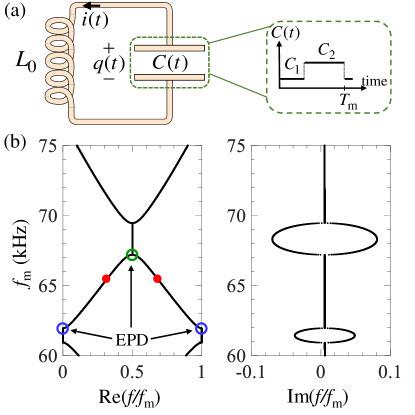
Figure 1: (a) Linear time-periodic LC resonator with a time-varying capacitor. The time-varying capacitance is a periodic piece-wise constant function as shown in the subset. (b) Dispersion diagram showing the real and imaginary parts of the eigenfrequencies of the resonator (i.e., the circuit’s resonance frequencies) versus modulation frequency $f_{\mathrm{m}}$ of the capacitance. Due to time-periodicity, an EPD resonance at frequency $f_{e0}$ has Fourier harmonics $f_{e0}+sf_{\mathrm{m}}$, with $s=0,\pm 1,\pm 2,...$.

An EPD of order two is the splitting point (or degenerate point) of two resonance frequencies and it emerges in systems when two or more eigenmodes coalesce into a single degenerate eigenmode, in both their eigenvalues and eigenvectors. The emergence of EPDs is associated with unique properties that promote several potential applications such as enhancing the gain of active systems (Othman et al., 2016a), lowering the oscillation threshold (Nada and Capolino, 2020) or improving the performance of laser systems (Veysi et al., 2018; Hodaei et al., 2014) or circuit oscillators (Oshmarin et al., 2019), enhancing circuits’ sensitivity at radio frequencies (Schindler et al., 2011; Chitsazi et al., 2017; Chen et al., 2018; Sakhdari et al., 2018, 2019) or at optical frequencies (Wiersig, 2014, 2016; Hodaei et al., 2017; Chen et al., 2017), etc.

EPDs emerge in EM systems using various methods: by introducing gain and loss in the system based on the concept of parity-time (PT-) symmetry (Bender and Boettcher, 1998; Stehmann et al., 2004; Schindler et al., 2011; Hodaei et al., 2014; Nada et al., 2018a; Chen et al., 2018; Sakhdari et al., 2018, 2019; Chitsazi et al., 2017; Wiersig, 2016, 2014; Hodaei et al., 2017; Chen et al., 2017), or by introducing periodicity (spatial or temporal periodicity) in waveguides (Nada et al., 2017; Othman et al., 2016b; Figotin and Vitebskiy, 2005; Nada et al., 2018b). Electronic circuits with EPD based on PT symmetry have been demonstrated in (Stehmann et al., 2004; Schindler et al., 2011) where the circuit is made of two coupled resonators with loss-gain symmetry, and only one precise combination of parameters leads to an EPD. The concept has been further elaborated in (Sakhdari et al., 2018; Chen et al., 2018) focusing on the high sensitivity of the EPD circuits introduced in (Stehmann et al., 2004; Schindler et al., 2011) to perturbations. Note that EPDs realized in PT-symmetric systems require at least two coupled resonators, and the precise knowledge and symmetry of gain and loss in the system. In contrast, in this paper we experimentally demonstrate EPDs that are directly induced via time modulation of a component in a single resonator (Kazemi et al., 2019b). An EPD induced by time modulation in a single resonator is easily tuned by just changing the modulation frequency of a component: this is a simple and viable strategy to obtain EPDs since the accurate change of a modulation frequency is common practice in electronic systems. Moreover, considering the fact that tuning of the modulation frequency is the key parameter to get an EPD, this strategy is also immune to tolerances in the values of commercially available inductors and capacitors.

In this paper we focus on the new scheme to obtain a second order EPD induced in a linear time periodic (LTP) system as introduced in (Kazemi et al., 2019b). Here EPDs are obtained by applying the time-periodic modulation to a system parameter (i.e., the capacitor) in a single resonator, and we provide an experimental demonstration of the existence of the LTP-induced EPD. Moreover, we show theoretically and experimentally how the resonance frequencies of a single EPD resonator are strongly perturbed by a tiny perturbation of its capacitor, and explore possible sensing applications of such phenomenon. We show that the system’s resonance frequency shift generated by a perturbed EPD follows the Puiseux fractional power expansion series (Welters, 2011), i.e., if $\delta$ is a perturbation to a second order EPD system, two resonances arise shifted by a quantity proportional to $\sqrt{\delta}$ from the EP degenerate resonance frequency. On the other hand, perturbed systems not operating at an EPD exhibit a frequency shift proportional to $\delta$, that is much smaller than $\sqrt{\delta}$ when $\left|\delta\right|\ll 1$. The theoretical predictions are in excellent agreement with the experimental demonstration, showing that tiny system perturbations can be detected by easily measurable resonance frequency shifts, even in the presence of electronic and thermal noise.

II Formulation of an LTP-induced EPD in a Single Resonator

We investigate resonances and their degeneracy in a linear time-periodic (LTP) LC resonator as shown in Fig. 1(a) where the time-varying capacitance is shown in the figure subset. This single-resonator circuit is supporting an EPD induced by the time-periodic variation. We consider a piece-wise constant time-varying capacitance $C(t)$ with period $T_{\mathrm{m}}$; we have chosen the piece-wise function to make the theoretical analysis easier, yet the presented analysis is valid for any periodic function. A thorough theoretical study of this type of temporally induced EPDs has been presented in (Kazemi et al., 2019b), here we focus on the energy transfer formulation of these EPDs, and we show the first practical implementation of the EPDs induced in LTP systems.

The state vector $\mathbf{\boldsymbol{\Psi}}(t)$ describing the system in Fig. 1 is two-dimensional (see Ref. (Kazemi et al., 2019b) for $N$-dimensional), i.e., $\mathbf{\boldsymbol{\Psi}}(t)=[q(t),i(t)]^{\mathrm{T}}$, where $\mathrm{T}$ denotes the transpose operator, $q(t)$ and $i(t)$ are the capacitor charge and inductor current, respectively. The temporal evolution of the state vector obeys the 2-dimensional first-order differential equation

$$\frac{\mathrm{d}\mathbf{\boldsymbol{\Psi}}(t)}{\mathrm{d}t}=\mathbf{\underline{M}}(t)\mathbf{\boldsymbol{\Psi}}(t),$$ (1)

where $\mathbf{\underline{M}}(t)$ is the $2\times 2$ system matrix. The 2-dimensional state vector $\boldsymbol{\Psi}(t)$ is derived at any time $t=nT_{\mathrm{m}}+\chi$ with $n$ being an integer and $0<\chi<T_{\mathrm{m}}$ as

$$\boldsymbol{\Psi}(t)=\underline{\boldsymbol{\Phi}}(\chi,0)\left[\underline{\boldsymbol{\Phi}}(T_{\mathrm{m}},0)\right]^{n}\boldsymbol{\Psi}(0),$$ (2)

where $\underline{\boldsymbol{\Phi}}(t_{2},t_{1})$ is the $2\times 2$ state transition matrix (Kazemi et al., 2019b) that translates the state vector from the time instant $t_{1}$ to $t_{2}$. The state transition matrix is employed to represent the time evolution of the state vector, hence we formulate the eigenvalue problem as (Kazemi et al., 2019b)

$$(\underline{\boldsymbol{\Phi}}-\lambda\underline{\mathbf{I}})\boldsymbol{\Psi}(t)=0.$$ (3)

The two eigenvalues are $\lambda_{p}=\exp(\mathrm{j}2\pi f_{p}T_{\mathrm{m}})$, $p=1,2$, where $f_{p}$ are the system resonant frequencies, with all their Fourier harmonics $f_{p}+sf_{\mathrm{m}}$, where $s$ is an integer and $f_{\mathrm{m}}=1/T_{\mathrm{m}}$ is the modulation frequency. Fig. 1(b) shows the dispersion diagram of the resonant frequencies varying modulation frequency $f_{\mathrm{m}}$, restricting the plot to frequencies in the range $0<f/f_{\mathrm{m}}<1$, which is called here as the fundamental Brillouin zone (BZ), adopting the language used in space-periodic structures. The two red circles in Fig. 1(b) corresponds to two general distinct resonant frequencies at $f$ and $-f+f_{\mathrm{m}}$ with positive real part. An EPD occurs when these two resonance frequencies coalesce at a given modulation frequency. At an EPD the transition matrix $\underline{\boldsymbol{\Phi}}$ is non-diagonalizable with a degenerate eigenvalue $\lambda_{e}$ (with corresponding eigenfrequency $\omega_{e}$) because the two eigenvalues and two eigenvectors coalesce. Two possibilities may occur because of the nature of the problem (time periodicity, because there are only two possible eigenmodes, and neglecting losses for a moment): the degenerate eigenvalue is either i) $\lambda_{e}=-1,$ corresponding to an eigenfrequency of $f_{e0}$ =$f_{\mathrm{m}}/2$ and its Fourier harmonics $f_{es}=f_{e0}+sf_{\mathrm{m}}$ shown with the green circles in Fig. 1(b), or ii) $\lambda_{e}=1$, corresponding to $f_{e0}=0$ and its Fourier harmonics $f_{es}=f_{e0}+sf_{\mathrm{m}}$ shown with a blue circle in Fig. 1(b). Therefore, in general an EPD resonance is characterized by the fundamental frequency $f_{e0}$ and all harmonics at $f_{es}=f_{e0}+sf_{\mathrm{m}}$ where $s=0,\pm 1,\pm 2,...$. Moreover, at an EPD the state transition matrix $\underline{\boldsymbol{\Phi}}$ is similar to a Jordan-Block matrix of second order, hence it has a single eigenvector, i.e., the geometrical multiplicity of the eigenvalue $\lambda_{e}$ is equal to 1 while its algebraic multiplicity is equal to 2. Considering the circuit parameters given in the next section including inductor small series resistance, an EPD occurs at $f_{\mathrm{m}}=62.7\,\mathrm{kHz}$, leading to a degenerate resonance frequency of $f_{e0}/f_{\mathrm{m}}=\mathrm{j}0.0041$ which corresponds to blue circle in Fig. 1(b). Another EPD occurs at $f_{\mathrm{m}}=67.7\,\mathrm{kHz}$, leading to a degenerate resonance frequency of $f_{e0}/f_{\mathrm{m}}=0.5+\mathrm{j}0.0038$ which corresponds to green circle in Fig. 1(b).

When $\lambda_{e}=-1$ and hence $f_{e0}$ =$f_{\mathrm{m}}/2$, i.e., for EPDs at the center of the BZ, the state transition matrix $\underline{\boldsymbol{\Phi}}$ has a trace of $-2$ (Kazemi et al., 2019b), so that we express $\left[\underline{\boldsymbol{\Phi}}(T_{\mathrm{m}},0)\right]^{n}$as (Richards, 1983)

$$\left[\underline{\boldsymbol{\Phi}}(T_{\mathrm{m}},0)\right]^{n}=\left(-1\right)^{n+1}[n\boldsymbol{\underline{\Phi}}(T_{\mathrm{m}},0)+(n+1)\mathbf{\underline{I}}],$$ (4)

where $\mathbf{\underline{I}}$ is the $2\times 2$ identity matrix. Thus, we reformulate (2) using (4) as

$$\boldsymbol{\Psi}(t)=\left(-1\right)^{n+1}[n\boldsymbol{\underline{\Phi}}(T_{\mathrm{m}},0)+(n+1)\mathbf{\underline{I}}]\boldsymbol{\underline{\Phi}}(\chi,0)\boldsymbol{\Psi}(0).$$ (5)

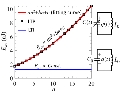
Figure 2: Comparison between the time-average energy stored in a lossless, linear time-invariant LC resonator (solid blue line) and the time-average energy stored in a linear time-periodic LC resonator operating at an EPD located at the edge of BZ (black square symbols) where $n$ is an integer representing the number of elapsed modulations periods. In the latter case the time-average energy grows with time, fitted by a second order polynomial curve (red solid line). The fitting coefficients are set as $a=0.01$, $b=0.23$, and $c=1.74$.

Similarly, for EPDs at the edge of the BZ, i.e., when $\lambda_{e}=1$ and $f_{e0}=0$, the transition matrix $\underline{\boldsymbol{\Phi}}$ has a trace equal to $2$, and (Richards, 1983)

$$\left[\underline{\boldsymbol{\Phi}}(T_{\mathrm{m}},0)\right]^{n}=n\boldsymbol{\underline{\Phi}}(T_{\mathrm{m}},0)-(n-1)\mathbf{\underline{I}},$$ (6)

hence

$$\boldsymbol{\Psi}(t)=[n\boldsymbol{\underline{\Phi}}(T_{\mathrm{m}},0)-(n-1)\mathbf{\underline{I}}]\underline{\boldsymbol{\Phi}}(\chi,0)\boldsymbol{\Psi}(0).$$ (7)

Because of the multiplication of the time-period step $n$, we conclude from Eqs. (5) and (7) that when the system is at the second order time-periodic induced EPD, the state vector grows linearly with time. This linear growth is expected and it is one of the unique characteristics associated with EPDs. This algebraic growth is analogous to the spatial growth of the state vector associated with the space-periodic EPDs (Othman et al., 2016a; Figotin and Vitebskiy, 2005).

The time-periodic LC tank considered in this section is not “isolated”. In such a system, the time-varying capacitor is in continuous interaction with the source of the time variation that is exerting work. This interaction leads to a net energy transfer into or out of the LC tank; at some operating modulation frequencies the system simply loses energy to the time-variation source, while at other operating modulation frequencies the LC tank receives energy from the source of time variation. This behavior is in contrast to the behavior of a time-invariant lossless LC tank where the initial energy in the system is conserved and the net energy gain or loss is zero. The average transferred energy into or out of the time-periodic LC tank can be calculated using the time-domain solution of the two-dimensional first-order differential equation (7). Figure 2 shows the calculated time-average energy transferred into a linear time-invariant (LTI) lossless LC tank (solid blue line) and into an LTP one operating at a second order EPD (black square symbols), where $n=0$ shows the average energy of the systems within the first period. The capacitor in both systems is initially charged with an initial voltage of $V_{C}(0^{-})=-50\,\mathrm{m}\mathrm{V}$. In the LTP system, the modulation frequency is adjusted to $f_{\mathrm{m}}=62.7\,\mathrm{kHz}$, so that it operates at the EPD denoted by the blue circles in Fig. 1(b). Note that the system is periodic, so that for an eigenfrequency $f_{p}$, there are also all the Fourier harmonics with frequencies $f_{p}+sf_{\mathrm{m}}$, where $s$ is an integer (Kazemi et al., 2019b). It is clear that the total energy in a lossless time-invariant LC resonator is constant over time while the average energy in the time-periodic LC resonator is growing at the EPD. This energy growth is quadratic in time since the state vector (i.e., capacitor charge and inductor current) of a periodically time-variant LC resonator experiencing an EPD grows linearly with time, as shown in Eqs. (5) and (7). Indeed, the solid red curve in Fig. 2 shows a second order polynomial curve fitted to the LTP LC resonator energy where the fitting coefficients are given in the figure caption. One may note from the figure that the average energy of the LTI and LTP systems are not equal at $n=0$ which might seem counter intuitive. In fact, at $n=0$ we show the average energy of the systems within the first time-period which is higher for the LTP system due to the energy transfer within that first period.

Note that the time-varying capacitance in our proposed scheme has some resemblance to the concept of parametric amplification (Ashkin et al., 1960; Cassedy and Oliner, 1963; R. C. Honey, 1960; Lee et al., 1997; Yamamoto et al., 2008). However, in our single resonator proposed scheme, we use time-periodicity of a system parameter to achieve an EPD (Kazemi et al., 2019b), and show high sensitivity of the degenerate resonance to system perturbations. In contrast, parametric amplifiers use time variation of a component as a non-conservative process to inject energy and generate amplification (which is not the case in our circuit), and generally possess low sensitivity to perturbations.

III Experimental Demonstration of an EPD and its Sensitivity to Perturbations

In this section we verify experimentally the key properties inferred from the degeneracy of resonances shown in the dispersion diagram in Fig. 1 and we observe some interesting physical properties by providing an initial charge to the capacitor and measure the triggered time domain natural response. The time varying LC tank with the time-periodic capacitor is implemented based on the scheme shown in Fig. 3(a). The time variation is carried out using a time-varying pump voltage $v_{p}(t)$ and a multiplier. Hence the voltage applied to the capacitor $C_{0}$ is equal to $v_{c}(t)=v(t)[1-v_{p}(t)/V_{0}]$, where $v(t)$ is the voltage of Node A with respect to the ground, and the term $V_{0}$ is a constant coefficient of the multiplier that is used to normalize its output voltage. Here we are interested in having an LC resonator with a time varying capacitor $C(t)$ seen by the current $i_{c}(t)$ exiting the inductor and by the voltage $v(t)$ at Node $A$, hence satisfying the two equations $q(t)=C(t)v(t)$ and $\mathrm{d}i_{c}/\mathrm{d}t=-v(t)/L_{0}=-q(t)/(L_{0}C(t))$. This leads to the definition of the time varying capacitance $C(t)\triangleq C_{0}(1-v_{p}(t)/V_{0})$ and to a LTP LC circuit described by Eq. (1) (see Supplement Material), which in turns leads to the time domain dynamics exhibiting EPDs as described in (Kazemi et al., 2019b).

In such a LTP LC circuit, the time variation behavior of the capacitance is dictated by the variation of the pump voltage $v_{p}(t)$, therefore to design the time-varying capacitance shown in Fig. 1(a) we apply a two level piece-wise constant pump voltage to the multiplier. The values of $C_{1}$ and $C_{2}$ are adjusted by properly choosing the voltages of the piece-wise constant pump $v_{p}(t)$ as discussed in the Supplement Material. We aim at designing the time-varying capacitor $C(t)$ with the values of $C_{1}=5\,\mathrm{n\mathrm{F}}$ and $C_{2}=15\,\mathrm{n\mathrm{F}}$. Hence, the parameters of the circuit are set as $C_{0}=10\,\mathrm{n\mathrm{F}}$, the two levels of the piece-wise constant time varying pump voltage as $v_{p}/V_{0}=\pm 0.5$, and the period of the pump voltage as $T_{\mathrm{m}}=20\,\mathrm{\mu s}$ with $50\%$ duty cycle. We verify the operation of this scheme using the finite difference time domain (FDTD) simulation implemented in Keysight ADS, where a constant capacitor $C_{0}$ is connected to the voltage multiplier. The time-varying capacitance, calculated as the ratio of the current passing through the capacitor $C_{0}$ to the time-derivative of the voltage at Node $A$, i.e., $i_{c}(t)/[\mathrm{d}v/\mathrm{d}t]$, is shown in Fig. 3(b). It is worth mentioning that in such a scheme, the high level of the pump voltage $v_{p}$ controls the value of the capacitance $C_{1}$ and the low level controls the value of the capacitance $C_{2}$.

Figure 3(c) illustrates the assembled circuit where the red dashed rectangle shows the implemented synthetic time-periodic capacitor $C(t)$. In this fabricated circuit we use a four-quadrant voltage output analog multiplier , a high stability and precision ceramic capacitor $C_{0}=10\,\mathrm{n\mathrm{F}}$, and an inductor $L_{0}=33\,\mu\mathrm{H}$ with low DC resistance $R_{DC}=108\,\mathrm{m\Omega}$, as specified in the Supplement Material. As shown in Sec. II, we expect the capacitor voltage of the time-periodic LC tank to grow linearly in time when operating at an EPD; however, in practice it will saturate to the maximum output voltage of the multiplier. Therefore, to avoid voltage saturation, we have implemented a reset mechanism to reset the resonator circuit, where the reset signal is a digital clock with $20\%$ duty cycle (i.e., $v_{reset}=2\,\mathrm{V}$ for 20% of its period and $v_{reset}=0\,\mathrm{V}$ otherwise) that allows the resonator circuit to run for the duration of the low voltage $v_{reset}=0\,\mathrm{V}$. During the reset time, the reset signal is high $v_{reset}=2\,\mathrm{V}$, and the resonator circuit is at pause. At the end of this time interval the capacitor is charged again with the initial voltage of $V_{C}(0^{-})=-50\,\mathrm{m}\mathrm{V}$ for the start of the next working cycle as detailed in the Supplement Material. The circuit is provided with $\pm 5\,\mathrm{V}$ DC voltage using a Keysight E3631A DC voltage supply. We use two Keysight 33250A function generators, one to generate a two level piece-wise constant signal with levels of $\pm 0.525\,\mathrm{V}$, duty cycle of $50\%$ and variable modulation frequency $f_{\mathrm{m}}$ as pump voltage $v_{p}(t)$ to generate the time-periodic capacitance $C(t)$. The other function generator provides the resonator’s reset signal, a two level piece-wise constant signal with levels of $2\,\mathrm{V}$ and $0\,\mathrm{V}$, with duty cycle of 20% and frequency of $1.1\,\mathrm{k}\mathrm{Hz}$ (much lower than $f_{\mathrm{m}}$).

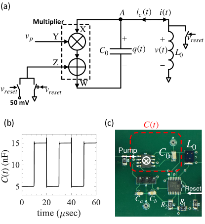
Figure 3: (a) Schematic of the LTP-varying LC resonator using the periodic pump voltage $v_{p}(t)$ and a multiplier. The reset switches are used in the implementation to avoid saturation and to add the initial voltage at the beginning of each “run” time. (b) Time domain simulations of the time-varying synthetic capacitance with period $T_{\mathrm{m}}$ seen from Node $A$ with respect to the ground. (c) Assembled circuit where the red dashed square shows the synthetic time-varying capacitor using the pump voltage and a multiplier. The circuit also consists of the inductor $L_{0}$, the reset circuit with switches, the regulating capacitors $C_{a}$ and $C_{b}$, and the circuitry to produce the initial voltage (see Supplement Material).

III.1 Dispersion diagram and time domain response

Figure 4(a) presents the dispersion diagram as a function of the capacitance’s modulation frequency $f_{\mathrm{m}}$, which is experimentally varied by adjusting the frequency of the pump voltage $v_{p}(t)$. The solid curve denotes the theoretical dispersion diagram whereas red square symbols represent the experimental results. The experimental results are obtained by calculating the resonance frequency of the circuit’s response for different modulation frequencies using Fourier transform of the time domain signal triggered by the initial voltage $V_{C}(0^{-})$ at each working cycle, where we used a Keysight DSO7104A digital oscilloscope to capture the time domain output signal. A good agreement is observed between the theoretical and experimental results, however, there is a slight frequency shift between the theoretical and experimental dispersion diagrams which is due to parasitic reactances, components’ tolerances and nonidealities in the fabricated circuit. Note that in Figure 4(a) we show only solutions in the first Brillouin zone defined here as $\mathrm{Re}(f)\in(0,f_{\mathrm{m}}).$ Since the system is time periodic, every mode is composed of an infinite number of harmonics with frequencies $f+sf_{\mathrm{m}}$, where $s$ is an integer. One can observe from the dispersion diagram that the time-periodic LC resonator operates at three different regimes depending on the modulation frequency. In the following we describe the three possible regimes of operation.

i) Real resonances: This is a regime where the system has two purely real oscillating frequencies (though in practice there is a small imaginary part due to the finite quality factor of the components). Point #2 with the magenta circle in Fig. 4(a) illustrates a mode part of this regime, with real resonance frequencies $f$, and all its harmonics $f+sf_{\mathrm{m}}$, where $s$ is an integer. The signal has also the resonance frequency at $-f+f_{\mathrm{m}}$, and hence also the harmonics at $-f+sf_{\mathrm{m}}$. This means that two resonance modes with frequencies $f$ and $-f+f_{\mathrm{m}}$ are allowed. Fig. 4(c) shows the corresponding time domain signal at $f_{\mathrm{m}}=66.5\,\mathrm{kHz}$ which corresponds to two almost-real resonance frequencies and their harmonics. As mentioned, the observed small exponential decay of the response is due to the finite quality factor of the components. In an ideal lossless system frequencies would be purely real.

ii) Unstable condition: This is a regime where the system has two complex resonance frequencies with imaginary parts of opposite signs (point #4 with the orange circle in Fig.4(a)). According to the time convention $\mathrm{e}^{\mathrm{j}\omega t}$, the state vector of the system corresponding to a complex resonance frequency with an imaginary part of negative sign shows an exponential growth, while the state vector corresponding to the resonance with an imaginary part with positive sign exhibits an exponential decay, hence it shows an unstable system. The exponentially growing behavior would be the dominant one and it is the one seen in the time domain response in Fig. 4(e) that would eventually saturate, if we did not include a reset circuit. In this case the modulation frequency of the pump voltage is set to $f_{\mathrm{m}}=71.5\,\mathrm{kHz}$.

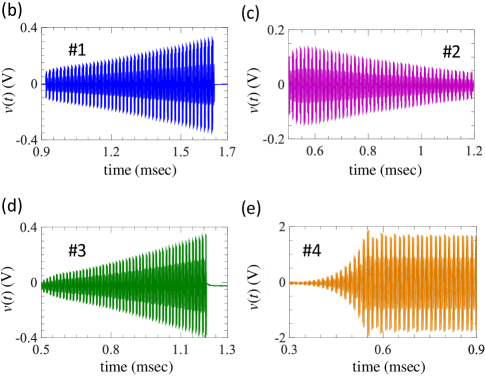
Figure 4: (a) Theoretical (solid lines) and experimental (square red symbols) results for the complex dispersion diagram showing the circuit’s resonance frequencies as a function of modulation frequency $f_{\mathrm{m}}$. (b-e) Time domain experimental results of the capacitor voltage at various modulation frequencies denoted by #1-4 in the dispersion diagram: (b) Exceptional point #1 denoted by the blue circle located at the edge of the BZ where the modulation frequency is $f_{\mathrm{m}}=62.8\,\mathrm{kHz}$. (c) Real-frequency resonance indicated by #2, denoted by the magenta circle, where the modulation frequency $f_{\mathrm{m}}=66.5\,\mathrm{kHz}$. (d) Exceptional point #3, denoted by the green circle, located at the center of the BZ where the modulation frequency is $f_{\mathrm{m}}=68.3\,\mathrm{kHz}$. (e) Unstable regime, point #4, denoted by an orange circle, represents two complex resonance frequencies, with opposite imaginary parts and real part equal to $f_{\mathrm{m}}/2$, where the modulation frequency is set to $f_{\mathrm{m}}=71.5\,\mathrm{kHz}.$ Note that due to time-periodicity, time domain signals have all Fourier harmonics $f+sf_{\mathrm{m}}$, with $s=0,\pm 1,\pm 2,...$.

iii) Exceptional points of degeneracy: An EPD is the point that separates the two previous regimes, where two frequency branches of the dispersion diagram (describing two independent resonance solutions) coalesce. Indeed at the EPD the two resonant modes of the system coalesce and, as discussed in the previous section, the state vector shows a linear growth with time yet the resonance frequencies are real (when neglecting the small positive imaginary part of the resonance frequency due to finite quality factor of the components). From the theoretical analysis and from the experimental results in Fig. 4(a) one may note two types of EPDs exist in a linear time-periodic system (Kazemi et al., 2019b). EPDs that exist at the center of the BZ, i.e., at $f_{e0}=0.5f_{\mathrm{m}}$, with Fourier harmonics located at $f_{es}=\left(0.5+s\right)f_{\mathrm{m}}$, where the integer $s$ denotes the harmonic number. An example of such a type of EPDs is observed at $f_{\mathrm{m}}=68.3\,\mathrm{kHz}$ and is denoted by point #3 with the green circle in Fig. 4(a). The measured time domain behavior of the circuit at this modulation frequency is shown in Fig. 4(d) where we clearly see the linear growth of the capacitor voltage. It grows until it reaches saturation or till the system is reset as described in the previous section. The other type of EPDs are those that exist at the edge of the BZ, i.e., at $f_{e0}=0$, with Fourier harmonics located at $f_{es}=sf_{\mathrm{m}}$. An example of this type of EPDs is denoted by point #1 with the blue circle at $f_{\mathrm{m}}=62.8\,\mathrm{kHz}$ in Fig. 4(a). The measured time domain behavior of the circuit at such an EPD is depicted in Fig. 4(b). Note that the oscillation of the time domain signal for an EPD at the edge of the BZ is due to the harmonics located at $sf_{\mathrm{m}}$.

One may observe that a standard “critically damped” LTI RLC circuit with two coinciding resonance frequencies is also an exceptional point, however, that point is characterized by two resonance frequencies with vanishing real part; hence, it is a different condition from what we describe in this paper.

III.2 High sensitivity to perturbations

Sensitivity of a system’s observable to a specific parameter is a measure of how strongly a perturbation to that parameter changes the observable quantity of that system. The sensitivity of a system operating at an EPD is boosted due to the degeneracy of the system eigenmodes. In the LTP system considered in this paper, a perturbation $\delta$ to a system parameter leads to a perturbed state transition matrix $\underline{\boldsymbol{\Phi}}$ and thus to perturbed eigenvalues $\lambda_{p}(\delta)$ with $p=1,2$. Therefore, the two degenerate resonance frequencies occurring at the EPD change significantly due to a small perturbation $\delta$, resulting in two distinct resonance frequencies $f_{p}(\delta)$, with $p=1,2$, close to the EPD resonance frequency. The two perturbed eigenvalues near an EPD are represented using a convergent Puiseux series (also called fractional expansion series) where the Puiseux series coefficients are calculated using the explicit recursive formulas given in (Welters, 2011). A first-order Puiseux approximation of $\lambda_{p}(\delta)$ is

$$\lambda_{p}(\delta)\approx\lambda_{e}+(-1)^{p}\alpha_{1}\sqrt{\delta}$$ (8)

where $\alpha_{1}$ is a coefficient that is either purely real or purely imaginary when losses can be neglected, and is given by

$$\alpha_{1}=\sqrt{-\frac{\frac{\mathrm{dD(0,\lambda_{e})}}{\mathrm{d}\delta}}{\frac{1}{2!}\frac{\mathrm{d^{2}D(0,\lambda_{e})}}{\mathrm{d}\lambda^{2}}}}.$$ (9)

where $D(\delta,\lambda)=\left[\mathrm{det}[\boldsymbol{\underline{\Phi}}(\delta)-\lambda\underline{\mathbf{I}}]\right]$. Since this is a second order polynomial in $\lambda$, the denominator of (9) is equal to unity. The perturbed complex resonance frequencies are approximately calculated as

$$f_{p}(\delta)\approx f_{es}\pm\mathrm{j}\frac{f_{\mathrm{m}}}{2\pi}(-1)^{p}\alpha_{1}\sqrt{\delta},$$ (10)

where the $\pm$ signs correspond to the cases with EPD either at the center ($f_{e0}=f_{\mathrm{m}}/2$ ) or edge ($f_{e0}=0$) of the BZ, respectively (we recall that in this paper the fundamental BZ is defined as $0\leq f/f_{\mathrm{m}}\leq 1$ ). Equation (10) is only valid for very small perturbations $\delta\ll 1$ and it is clear that for such a small perturbation the resonance frequencies $f_{p}$ change dramatically from the degenerate resonance $f_{es}$ due to the square root function. In other words the EPD is responsible for the square root dependence $\triangle f=f_{p}(\delta)-f_{es}\propto$$\sqrt{\delta}$. Now, let us assume that the perturbation $\delta$ is applied to the value $C_{1}$ of the time-varying capacitor, and the perturbed $C_{1}$ is expressed as $(1+\delta)C_{1}$. Considering an unperturbed LTP LC resonator as shown in the subset of Fig. 1(a), the system has a measured EPD resonance at a modulation frequency $f_{\mathrm{m}}=62.8\,\mathrm{kHz}$ for the parameter values given in section III. This EPD resonance frequency is at $f_{e0}=0\,\mathrm{Hz}$, corresponding to point #1 (blue circle) in the dispersion diagram shown in Fig. 4(a), and at all its Fourier harmonics $f_{es}=f_{e0}+sf_{\mathrm{m}}$. By looking at the spectrum of the measured capacitor voltage we observe that among the various harmonics of such EPD resonance, the frequency of $\mathrm{Re}(f_{e6})=6f_{\mathrm{m}}=374.2\,\mathrm{kHz}$ has a dominant energy component, hence it is the one discussed in the following. The theoretical and experimental variations in the real part of the two perturbed resonance frequencies due to a perturbation $\delta\ll 1$ in the the time-variant LC circuit are shown in Fig. 5. Only the results for positive variations of $\delta$ are shown here, hence the resonances move in the directions where they are purely real (though the presence of small losses would provide a small imaginary part in the resonance frequency). The solid blue curve, dashed red curve, and green symbols denote the calculated-exact (solutions of Eq. (3) explained in Sec. II), Puiseux series approximation, and the experimentally observed resonance frequencies, respectively when varying $\delta$.

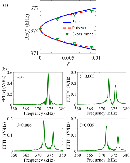
Figure 5: (a) Proof of exceptional sensitivity. Experimental and theoretical changes in the real part of the two resonance frequencies $f_{p}$ due to a positive relative perturbation $\delta$ applied to the capacitance $C_{1}$ of the time-varying capacitor (i.e., as $(1+\delta)C_{1}$). The two real frequencies greatly depart from the EPD frequency around 374 kHz even for very small variation of the capacitance following the fractional power expansion $\triangle f=f_{p}(\delta)-f_{es}\propto$$\sqrt{\delta}$. The solid blue line, dashed red line and green symbols represent the calculated-exact, Puiseux series approximation, and experimental resonance frequencies of the LTP LC circuit shown in the Fig. 1(a). The EPD frequency around 374 kHz corresponds to point #1 (blue circle) at the edge of the BZ in Fig. 4(a). (b) Fast Fourier transform of the measured capacitor voltage $v(t)$, obtained at the EPD point and at three different perturbations of the capacitor $C_{1}$. The four spectra correspond to the experimental green triangles in Fig. (a) and they show the resonance frequency shifts due to the capacitor’s perturbation.

The coefficient $\alpha_{1}$ in the Puiseux series is calculated to be $\alpha_{1}=\mathrm{j}2.65$ which according to the fractional expansion in Eq. (10) it implies only change of the real part of the resonance frequency for a positive perturbation $\delta>0$ while the imaginary part is constant. The three curves are in excellent agreement for small perturbations, showing also the remarkable agreement of the experimental results with the theoretical ones indicating that this is a viable practical solution to make ultra-sensitive sensors. The perturbation $\delta$ (the relative change in capacitance $C_{1}$) is experimentally introduced through changing the positive voltage level of the pump voltage $v_{p}(t)$. In such a design, each $5\,\mathrm{mV}$ change in the positive level of the pump voltage will result in $1\%$ change of the $C_{1}$ capacitor value corresponding to $\delta=0.01$ (see the Supplement Material). The experimental results (green triangles) in Fig. 5(a) represent the peaks of the fast Fourier transform (FFT) of the measured voltage $v(t)$ of Node A with respect to the ground. The FFT in Fig. 5(b) is taken over the time domain interval corresponding to the “ON” state of the circuit, i.e., during 727$\,\mathrm{\mu s}$ which correspond to 80% of 1.1 KHz, while $v_{reset}=0\,\mathrm{V}$(see Supplemental Material). The results in Fig. 5 demonstrate theoretically and experimentally that for a small perturbation $\delta$, the real part of the resonance frequency is significantly changed and that it can be easily detected even in real noisy electronic systems. Indeed, the spectral width of the measured peaks is small enough to even distinguish the difference between $\delta=0$ and $\delta=0.003$. We also increased the repetition frequency and observed the linear-growth saturation of the system under the EPD regime, and by doing the Fourier transform of the time domain signal in the four cases over a time window of length 2 ms (which included the saturation regime); this provided the same results provided in Fig. 5(a) and (b). This latter test showed that the circuit can be operated even including the saturation regime and it would still provide enhanced sensitivity to perturbation. In conclusion, these experimental results unequivocally demonstrate the exceptional sensitivity of the proposed system operating at an EPD and the practicality of the LTP-resonator circuit to conceive a new class of extremely sensitive sensors.

III.3 Discussion

A perturbation of the single resonator with an LTP component (for instance a perturbation of the $C_{1}$ value of the time-varying capacitance), perturbs the system away from the EPD. In absence of loss, such a perturbation results in two real-valued, shifted resonance frequencies$f_{p}(\delta)$. When losses are present the EPD frequency $f_{es}$ is slightly complex (see Sec. II) and the two frequency shifts $\triangle f=f_{p}(\delta)-f_{es}$ are approximately real valued. Instead, in a two-coupled resonator system based on PT symmetry operating at an EPD, perturbing one of the capacitors, for instance the one on the lossy (sensing) side, results in two complex resonance frequencies (the value of $\alpha_{1}$ in that case would be complex). The reasons of why the two shifted frequencies are complex in a coupled-resonator circuit relies on the fact that the asymmetry in the capacitances (due to the perturbation) disqualifies the system as PT-symmetric and hence the resonance frequencies are no longer real-valued. However, in the sensitive two-coupled PT-symmetric resonator system presented in (Chen et al., 2018; Sakhdari et al., 2018) a (sensing) capacitance perturbation resulted in two real resonance frequencies because in that system PT symmetry was maintained by manually changing the capacitance on the gain side of the circuit (using a varactor) to exactly balance the capacitance perturbation on the sensing (lossy) side of the circuit.

Nevertheless, in many practical applications, a prior knowledge of how much the sensing capacitance is perturbed is not available since the amount of capacitance perturbation depends on the physical (or chemical/biological) quantity to be measured, and the perturbed frequencies would not be real. The reason of this striking difference between the performance of a PT-symmetric coupled resonator circuit and the proposed LTP single resonator circuit rely on the fact that in the PT symmetry case the Puiseux series coefficient $\alpha_{1}$ for one varying capacitance is complex whereas in our case the Puiseux series coefficient $\alpha_{1}$ for the varying capacitance is either purely real or purely imaginary, depending on the EPD point considered in the dispersion diagram in Fig. 1.

Another important consideration which shows a possible advantage of our proposed sensing scheme is that the capacitance and inductance values of electronic components are not precisely known, i.e., commercially available components have prescribed tolerances (e.g., 1%, 2%, 5%). This uncertainty affects the exact occurrence of the EPD in a PT-symmetric system and in turn it would affect its sensitivity to perturbations. On the contrary, in our case, the tuning of the modulation frequency would generate an EPD regardless of the precise components values. Note that the exact frequency at which the EPD occurs is not important in sensing applications since the sensitivity is associated to the shift from such an EPD frequency, and only the precise measurement if the shift is required.

Finally, it is important to note that electronic and thermal noise in the proposed circuit did not compromise the capability to experimentally verify the high sensitivity of the LTP single-resonator circuit to a system perturbation, as clearly demonstrated in Fig. 5. The resonance peaks in Fig. 5(b) obtained from the measurement of the time domain voltage waveform are very distinguishable from each other, and their spectral width is much narrower than the frequency shift associated to even 0.3% variation of the perturbed capacitance. Therefore, this paper shows the experimental proof of the existence of EPDs in a single resonator circuit with a LTP modulation of a component, and also the high sensitivity of the system’s resonances to perturbations, regardless of the presence of noise. Despite the topic of using EPDs to enhance sensitivity is still subject to some debate, see for instance (Langbein, 2018; Zhang et al., 2019b; Lau and Clerk, 2018; Wiersig, 2020a, b; Xiao et al., 2019), our experimental results clearly show that in some respect it is possible to observe the special sensitivity provided by the square root behavior $\sqrt{\delta}$ when $\left|\delta\right|\ll 1$, proper of an EPD, even in presence of realistic noise in the electronic system. Sensitivity to perturbations could be further enhanced by understanding how the parameter $\alpha_{1}$ could be increased by an improved design of the system’s components.

IV Conclusion

We have shown the first practical and experimental demonstration of exceptional points of degeneracy (EPDs) directly induced via time modulation of a component in a single resonator. This is in contrast to EPDs realized in PT-symmetric systems that would require two coupled resonators instead of one, and the precise knowledge of gain and loss in the system as well as the values of L and C components to have a high quality PT-symmetric resonator. Instead, in our proposed LTP-based scheme we have shown that controlling the modulation frequency of a component in a single resonator is a viable strategy to obtain EPDs since varying a modulation frequency in a precise manner is common practice in electronic systems. The occurrence of a second-order EPD has been shown theoretically and experimentally in two ways: by reconstructing the dispersion diagram of the system resonance frequencies, and by observing the linear growth of the capacitor voltage. We have also experimentally demonstrated how such a temporally induced EPD renders a simple LC resonating system exceptionally sensitive to perturbations of the system capacitance, and how the measurement of the shifted frequencies is robust with respect to the presence of noise. Therefore, the excellent agreement between measured and theoretical sensitivity results demonstrate that the new scheme proposed in this paper is a viable solution for enhancing sensitivity, paving the way to a new class of ultra sensitive sensors that can be applied to a large variety of problems where the occurrence of small quantity of substances shall be detected.

It is important to observe that there are fundamental differences between using the PT symmetry based circuit discussed in (Schindler et al., 2011; Sakhdari et al., 2018; Chen et al., 2018) and the LTP circuit demonstrated in this paper, in detecting small perturbations of a circuit element: (i) in the PT-symmetric based circuit with two resonators, when the capacitance on one of the resonators is varied the circuit is not PT-symmetric anymore and the two perturbed resonance frequencies caused by the change of that capacitance are always complex-valued; instead in our case, a perturbation of the capacitance leads to two real-valued frequency shifts from the EPD one, and this may have very important implications in sensing technology; (ii) our EPD is easy to obtain by simply modifying the modulation frequency; (iii) the capability to obtain EPDs is not sensitive to tolerances of realistic components since we only need to tune the modulation frequency to obtain an EPD (this is not true in PT symmetry systems where multiple components needs to have precise values at the same time).