Speeding-up Ab Initio Molecular Dynamics with Hybrid Functionals using Adaptively Compressed Exchange Operator based Multiple Timestepping

Abstract

Ab initio molecular dynamics (AIMD) simulations using hybrid density functionals and plane waves are of great interest owing to the accuracy of this approach in treating condensed matter systems. On the other hand, such AIMD calculations are not routinely carried out since the computational cost involved in applying the Hartree Fock exchange operator is very high. In this work, we make use of a strategy that combines adaptively compressed exchange operator formulation and multiple time step integration to significantly reduce the computational cost of these simulations. We demonstrate the efficiency of this approach for a realistic condensed matter system.

Ab initio molecular dynamics (AIMD) simulations with density functional theory (DFT) and plane wave (PW) basis set are the methods of choice in studying structural and dynamic properties of condensed matter systems.Marx and Hutter (2009) Usage of density functionals at the level of Generalized Gradient Approximation (GGA) is commonplace for these simulations because more than a million energy and force evaluations are computationally achievable by taking advantage of parallel programs and parallel computing platforms. Contrarily, hybrid density functionals are preferred over GGA functionals for improved accuracy in AIMD simulations.Todorova et al. (2006); Zhang et al. (2011); DiStasio Jr. et al. (2014); Ambrosio, Miceli, and Pasquarello (2016) Computations of energy and gradients at the hybrid functional level using PW basis set have prohibitively high computational cost resulting from the application of the exact exchange operator on each of the occupied orbitals. One of the ways to increase the efficiency of such AIMD simulations is by making use of multiple time step (MTS) algorithmsTuckerman, Martyna, and Berne (1990); Tuckerman, Berne, and Martyna (1992) among others.Wu, Selloni, and Car (2009); DiStasio Jr. et al. (2014); Gygi and Duchemin (2013); Dawson and Gygi (2015); Ratcliff et al. (2018); Mandal et al. (2018) In this respect, the reversible reference system propagator algorithm (r-RESPA)Tuckerman, Berne, and Martyna (1992) has been used by several authors.Guidon et al. (2008); Liberatore, Meli, and Rothlisberger (2018); Fatehi and Steele (2015) In the r-RESPA MTS approach, artificial time scale separation in the ionic force components due to computationally intensive Hartree Fock exchange (HFX) contribution and the computationally cheaper rest of the terms is made.Guidon et al. (2008); Liberatore, Meli, and Rothlisberger (2018) In this manner, MTS scheme allows us to compute HFX contributions less frequently compared to the rest of the contributions to the force, thereby reducing the overall computational cost in performing AIMD simulations.

Here we propose a new way to take advantage of the r-RESPA scheme for performing AIMD using hybrid functionals and PWs. This scheme is based on the recently developed adaptively compressed exchange (ACE) operator approach.Lin (2016); Hu et al. (2017) We exploited some property of the ACE operator to artificially split the ionic forces into fast and slow.

The self consistent field (SCF) solution of hybrid functional based Kohn-Sham (KS) DFT equations requires application of the exchange operator ${\mathbf{V}}_{\rm X}=-\sum_{j}^{N_{\rm orb}}\frac{|\psi_{j}\rangle\langle\psi_{j}|}{r_{12}}$ on each of the KS orbitals $|\psi_{i}\rangle$:

$${\mathbf{V}}_{\rm X}|\psi_{i}\rangle=-\sum_{j}^{N_{\rm orb}}|\psi_{j}\rangle\left\langle\psi_{j}\left|\left(r_{12}\right)^{-1}\right|\psi_{i}\right\rangle,\enspace~{}~{}i=1,....,N_{\rm orb}\enspace.$$ (1)

Here, $N_{\rm orb}$ is the total number of occupied orbitals. The evaluation of $\left\langle\psi_{j}\left|\left(r_{12}\right)^{-1}\right|\psi_{i}\right\rangle$ is usually done in reciprocal spaceChawla and Voth (1998); Wu, Selloni, and Car (2009) using Fourier transform (FT). If $N_{\rm G}$ is the total number of PWs, the computational cost for doing FT scales as $N_{\rm G}\log N_{\rm G}$ on using fast Fourier transform (FFT) algorithm. The total computational cost scales as $N_{\rm orb}^{2}N_{\rm G}\log N_{\rm G}$,Chawla and Voth (1998) as operation of ${\mathbf{V}}_{\rm X}$ on all the KS orbitals requires $N_{\rm orb}^{2}$ times evaluation of $\left\langle\psi_{j}\left|\left(r_{12}\right)^{-1}\right|\psi_{i}\right\rangle$.

In the recently developed ACE operator formulation,Lin (2016) the full rank ${\mathbf{V}}_{\rm X}$ operator is approximated by the ACE operator ${\mathbf{V}}_{\rm X}^{\rm ACE}=-\sum_{k}^{N_{\rm orb}}|P_{k}\rangle\langle P_{k}|$ using a low rank decomposition. Here, $\{|P_{k}\rangle\}$ is the set of ACE projection vectors which can be computed through a series of simpler linear algebra operations. Now, the evaluation of the action of ${\mathbf{V}}_{\rm X}^{\rm ACE}$ operator on KS orbitals can be done with $N_{\rm orb}^{2}$ number of simpler inner products as

$${\mathbf{V}}_{\rm X}^{\rm ACE}|\psi_{i}\rangle=-\sum_{k}^{N_{\rm orb}}|P_{k}\rangle\left\langle P_{k}|\psi_{i}\right\rangle,\enspace~{}~{}i=1,....,N_{\rm orb}\enspace.$$ (2)

The advantage of the ACE approach is that the cost of applying the ${\mathbf{V}}_{\rm X}^{\rm ACE}$ operator on each KS orbitals is much less as compared to ${\mathbf{V}}_{\rm X}$ operator. At the first SCF step, ${\mathbf{V}}_{\rm X}^{\rm ACE}$ operator can be constructed through the computation of $\{{\mathbf{V}}_{\rm X}|\psi_{i}\rangle\}$, which is the costliest step ($N_{\rm orb}^{2}$ times evaluation of $\left\langle\psi_{j}\left|\left(r_{12}\right)^{-1}\right|\psi_{i}\right\rangle$). As HFX has only a minor contribution to the total energy, an approximate energy computation is possible by using the previously constructed ${\mathbf{V}}_{\rm X}^{\rm ACE}$ operator without updating it for the rest of the SCF iterations. It is again stressed that, once the ${\mathbf{V}}_{\rm X}^{\rm ACE}$ operator is constructed, its low rank structure allows the easy computation of $\{{\mathbf{V}}_{\rm X}^{\rm ACE}|\psi_{i}\rangle\}$ in the subsequent SCF iterations. We exploit this property of the ACE operator to combine with the r-RESPA scheme.

In the r-RESPA method,Tuckerman, Berne, and Martyna (1992) symmetric Trotter factorization of the classical time evolution operator is carried out. Let that ionic force can be decomposed into slow and fast components as $F_{K}=F_{K}^{\rm fast}+F_{K}^{\rm slow}$, $K=1,\cdots,3N$, for a system containing $N$ atoms. In this case, the Liouville operator $L$ can be written as

$$iL=iL^{\rm fast}_{1}+iL^{\rm fast}_{2}+iL^{\rm slow}\enspace,$$ (3)

with

$$iL^{\rm fast}_{1}=\sum_{K=1}^{3N}\left[\dot{X}_{K}\frac{\partial}{\partial{X}_{K}}\right],~{}~{}iL^{\rm fast}_{2}=\sum_{K=1}^{3N}\left[F_{K}^{\rm fast}\frac{\partial}{\partial{P}_{K}}\right]$$ (4)

and

$$iL^{\rm slow}=\sum_{K=1}^{3N}\left[F_{K}^{\rm slow}\frac{\partial}{\partial{P}_{K}}\right]\enspace.$$ (5)

Here, $\{X_{K}\}$ and $\{P_{K}\}$ are the Cartesian coordinates and the conjugate momenta of the particles. Using symmetric Trotter factorization, we arrive at

$$\begin{split}\exp(&iL\Delta t)\approx\exp\left(iL^{\rm slow}\frac{\Delta t}{2}\right)\\ &\times\left[\exp\left(iL^{\rm fast}_{2}\frac{\delta t}{2}\right)\exp\left(iL^{\rm fast}_{1}\delta t\right)\exp\left(iL^{\rm fast}_{2}\frac{\delta t}{2}\right)\right]^{n}\\ &\times\exp\left(iL^{\rm slow}\frac{\Delta t}{2}\right)\enspace.\end{split}$$ (6)

Here, the large time step $\Delta t$ is chosen according to the time scale of variation of slow forces ($\{F_{K}^{\rm slow}\}$) and the smaller time step $\delta t=\Delta t/n$ is chosen according to the time scale of fast forces ($\{F_{K}^{\rm fast}\}$).

Now, we split the contribution of ionic forces from the HFX part as

$$F^{\rm hybrid}_{K}=F^{\rm ACE}_{K}+\Delta F_{K}\enspace,\enspace K=1,\cdots,3N\enspace$$ (7)

with $\Delta F_{K}=\left(F^{\rm hybrid}_{K}-F^{\rm ACE}_{K}\right)$. Here, $\mathbf{F}^{\rm hybrid}$ is the ionic force computed with the full rank exchange operator ${\mathbf{V}}_{\rm X}$. The term $\mathbf{F}^{\rm ACE}$ is the ionic force calculated using the low rank ${\mathbf{V}}_{\rm X}^{\rm ACE}$ operator. In Figures 1(a) and (b) we have shown the components of the $\mathbf{F}^{\rm ACE}$ and $\Delta\mathbf{F}$ for a realistic molecular system, where $\mathbf{V}_{\rm X}^{\rm ACE}$ is calculated once at the beginning of a SCF while kept fixed during the remaining SCF cycles. The clear difference in the time scale at which the two forces are varying allowed us to use $\mathbf{F}^{\rm ACE}$ as the fast ionic force and $\Delta\mathbf{F}$ as the slow ionic force, and combine it with the r-RESPA algorithm. Here, the longer time step $\Delta t$ is chosen according to the time scale of variation of the computationally costly slow forces, whereas the smaller time step $\delta t$ is taken as per the time scale of fast forces that are cheaper to compute. In this way, we get the required speed-up using r-RESPA scheme to perform hybrid functional based AIMD simulations. A flowchart of the method is given in Figure 2 and 3.

Benchmark calculations were carried out for a 32 water system where the molecules were taken in a supercell of dimensions 9.85 Å$\times$9.85 Å$\times$9.85 Å with water density $\sim$1 g cm^-3. Calculations were carried out employing the CPMD programHutter et al. where the proposed method has been implemented. The PBE0Adamo and Barone (1999) exchange correlation functional was employed together with the norm-conserving Troullier-Martin type pseudopotentials.Troullier and Martins (1991) A PW cutoff energy of 80 Ry was used. Born-Oppenheimer molecular dynamics (BOMD) simulations were carried out to perform MD simulations at the microcanonical (NVE) and canonical (NVT) ensembles. In order to perform canonical ensemble AIMD simulation, we employed Nosé–Hoover chain thermostatsMartyna, Klein, and Tuckerman (1992) and the temperature of the system was set to 300 K. Addition of thermostats also helps to eliminate any resonance effects originated with the use of large time step.Ma, Izaguirre, and Skeel (2003) At every MD steps, wavefunctions were converged till the magnitude of maximum wavefunction gradient reached below $1\times 10^{-6}$ au. The initial guess for the wavefunctions at every MD step was obtained using Always Stable Predictor Corrector Extrapolation schemeKolafa (2004) of order 5.

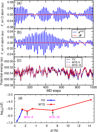
Figure 1: Test results for 32-water system using PBE0 functional: One of the components of $\mathbf{F}^{\rm ACE}$ and $\Delta\mathbf{F}$ on an arbitrarily chosen (a) oxygen and (b) hydrogen atoms; (c) Comparison of potential energy during VV, MTS-5 and MTS-15 simulations in NVE ensemble; (d) $\log_{10}(\Delta E)$ for different $\Delta t$ values in VV and MTS simulations calculated from 5 ps long trajectories.

Figure 2: Flowchart of the MTS propagation scheme proposed in this work.

Figure 3: Flowchart showing the steps involved in computing $\mathbf{F}^{\rm ACE}$.

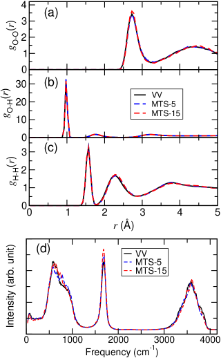
Figure 4: Radial distribution functions (RDFs) for bulk water simulation from VV, MTS-5 and MTS-15 trajectories at the level of PBE0: (a) O-O, (b) O-H, and (c) H-H. (d) Power spectrum of the same system computed from VV, MTS-5 and MTS-15 trajectories.

Table 1: Comparison of various quantities for VV, MTS-5 and MTS-15 simulations in NVE ensemble.

Method	$\log_{\rm 10}(\Delta E)$	${\Delta U}$/(au)	$t_{\rm CPU}/(s)$	speed-up
VV	-6.8	0.0	258	1
MTS-5	-5.4	5.9$\times 10^{-4}$	64	4
MTS-15	-5.2	1.9$\times 10^{-3}$	38	7

Table 2: CPU time for various stages of the program.

CPU time per SCF using ${\mathbf{V}}_{\rm X}$ operator	24 s
CPU time per SCF using ${\mathbf{V}}_{\rm X}^{\rm ACE}$ operator	0.1 s
Average CPU time for the construction of ${\mathbf{V}}_{\rm X}^{\rm ACE}$ at the beginning of every MD step	24 s

To benchmark our implementation, we first compared the fluctuations in total energy using conventional velocity Verlet (VV) integrator and MTS runs (MTS-n) with $n=\Delta t/\delta t$, and $\delta t\approx 0.5$ fs for 32-water in a periodic box treated by PBE0 functional. The magnitude of the total energy ($E$) fluctuations is measured by

$$\Delta E=\left<\left|\frac{E-\left\langle E\right\rangle}{\left\langle E\right\rangle}\right|\right>\enspace,$$ (8)

where $\left<\cdots\right>$ specifies time average. In the case of VV runs, $\log_{10}(\Delta E)$ increases with higher $\Delta t$ corresponding to the increase in total energy fluctuations as shown in Figure 1(d). We also observed that the use of a timestep greater than 1.4 fs in VV runs leads to unstable trajectories with breaking of O-H covalent bonds. In MTS-n runs, we kept the inner timestep $\delta t$ fixed at $\sim$0.5 fs and varied outer timestep $\Delta t=n\,\delta t$. The quality of the energy conservation in these runs depends on the value of $n$, which determines how large the outer timestep is compared to the inner timestep. It is clear from Figure 1(d) that MTS-n runs with $n$ up to 15 have total energy conservation comparable to VV run using a timestep $1.4$ fs. Although the MTS-30 run (with $\Delta t=14.4$ fs) was showing higher total energy fluctuation, it was able to generate stable MD trajectories. Notably, we observed good accuracy in MTS runs with $n=15$ (i.e. MTS-15); (see Table 1).

In order to show the correctness of our proposed MTS scheme, we compared the fluctuation in potential energy for VV, MTS-5 and MTS-15 runs for a short initial time period for the 32-water system (before the trajectories deviate due to growing numerical differences) in Figure 1(c); see also Table 1. All these simulations were started with the same initial conditions. We find that potential energy computed from the MTS-5 and MTS-15 trajectories are closely following the potential energy from the VV run.

As next, we carried out NVT simulations for the same system and computed static and dynamical properties of bulk water. In particular, we calculated partial radial distribution functions (RDFs) and the power spectrum; see Figure 4. It is clear that the RDFs from the MTS simulations are in excellent agreement with those from the VV run (Figure 4 a,b and c). Also, the power spectrum computed from these calculations are in excellent agreement (Figure 4 d). Thus, we conclude that our MTS scheme gives accurate description of the structural and dynamical properties.

We now compare the average computational time per MD step ($t_{\rm CPU}$) for MTS-n and VV runs; see Table 1 and 2. We have achieved a speed-up of $\sim$4 fold for the 32-water system with MTS-5 as compared to the VV run. At the same time, with MTS-15 we could achieve a speed-up of $\sim$7 fold. It is crucial to notice that application of $\mathbf{V}_{\rm X}^{\rm ACE}$ operator at every SCF cycle in place of the exact exchange operator $\mathbf{V}_{\rm X}$ gives a speed-up of $\sim$240 (See Table 2). However, construction of $\mathbf{V}_{\rm X}^{\rm ACE}$ operator, which is done only once in every MD time step, is computationally expensive (and has the same computational cost of applying the exact exchange operator). Thus in this method, construction of $\mathbf{V}_{\rm X}^{\rm ACE}$ remains as the computational bottleneck.

In conclusion, we presented a new scheme in using r-RESPA to perform hybrid functional based AIMD simulations with PW basis set. This involves artificial splitting in the nuclear forces envisaged by the recently developed ACE approach. Our benchmark results for liquid water show that stable and accurate MD trajectories can be obtained through this procedure. For the specific case of 32-water system, a computational speed-up up to 7 could be obtained. We hope that this approach will enable us to compute long accurate AIMD trajectories at the level of hybrid DFT. Further systematic improvement can be made to speed-up this approach, in particular the construction of ACE operator,Carnimeo, Baroni, and Giannozzi (2019) and is beyond the scope of this work.