dpi
A mathematical model describing the localization and spread of influenza A virus infection within the human respiratory tract
Abstract
Within the human respiratory tract (HRT), viruses diffuse through the periciliary fluid (PCF) bathing the epithelium, and travel upwards via advection towards the nose and mouth, as the mucus escalator entrains the PCF. While many mathematical models (MMs) to date have described the course of influenza A virus (IAV) infections in vivo, none have considered the impact of both diffusion and advection on the kinetics and localization of the infection. The MM herein represents the HRT as a one-dimensional track extending from the nose down to a depth of , wherein stationary cells interact with the concentration of IAV which move along within the PCF. When IAV advection and diffusion are both considered, the former is found to dominate infection kinetics, and a 10-fold increase in the virus production rate is required to counter its effects. The MM predicts that advection prevents infection from disseminating below the depth at which virus first deposits. Because virus is entrained upwards, the upper HRT sees the most virus, whereas the lower HRT sees far less. As such, infection peaks and resolves faster in the upper than in the lower HRT, making it appear as though infection progresses from the upper towards the lower HRT. When the spatial MM is expanded to include cellular regeneration and an immune response, it can capture the time course of infection with a seasonal and an avian IAV strain by shifting parameters in a manner consistent with what is expected to differ between these two types of infection. The impact of antiviral therapy with neuraminidase inhibitors was also investigated. This new MM offers a convenient and unique platform from which to study the localization and spread of respiratory viral infections within the HRT.
1 Introduction
Mathematical models (MMs) of influenza A virus (IAV) infection kinetics are mainly based on ordinary differential equations (ODEs) that describe the time evolution of infection (virus as a function of time) with the implicit assumption that all cells see all virus and vice-versa, as discussed in several reviews [23, 10, 29]. A different approach from ODE MMs is to use agent-based MMs which treat the dynamics of each cell, and even each virus, individually and track local cell-virus interactions [71, 7, 5]. Such MMs are computationally intensive, restricting the number of cells, and therefore the area, which can be represented, and often lack support or validation in the form of experimental localization data [7, 4, 50]. Infection localization can also be modelled by dividing the human respiratory tract (HRT) into compartments corresponding to different regions of the HRT, where each compartment has different parameters based upon physiological differences [62].
IAV infection spread faces a tremendous physical, spatial barrier in the form of the thick mucus layer which lines the HRT, trapping and carrying free virions rapidly upwards towards the nose and throat and out of the HRT [26]. This physical clearing process is typically taken somewhat into account in non-spatial ODE MMs via a term for the exponential clearance of virions. This simplification, however, does not account for the fact that not all cells will have equal exposure to the virus: cells that are downstream of the mucus flow (higher in the HRT) will have greater exposure to virus than those upstream, located deeper within the HRT. To our knowledge, the effect of virus advection due to entrainment by the mucus layer on IAV infection localization and spread within the HRT has never been evaluated.
In this work, a spatiotemporal MM for the spread of IAV infection within the HRT using partial differential equations (PDEs) is constructed. Through its one-dimensional representation of the HRT, the MM is used to study the effect of viral transport modes on the course of an IAV infection in vivo. Via the addition of only two additional spatial parameters whose value is relatively well-established, namely the rate of diffusion and advection of virions, the MM able to produce a richer range of IAV kinetics. The effect of cellular regeneration and a simplified immune response are also considered. The PDE MM is also used to explore differences in the kinetics of IAV infection, in the absence and presence of antiviral therapy, for IAV infection with either a seasonal or an avian-adapted strain, with the latter being typically more severe [56].
2 Results
2.1 A spatial MM for IAV in the HRT
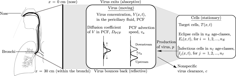
In the proposed spatial MM, the HRT is represented as a one-dimensional tract running along the -axis indicating the depth within the HRT, with located at the top of the HRT (nose), and terminating somewhere within the bronchi [60, 70], as illustrated in Figure 1. It is an extension of the ‘standard’ MM for IAV in vitro [55, 68, 59] which adds: (1) the diffusion of virions through the periciliary fluid (PCF) which lies between the cells’ apical surface and the thick mucus blanket which lines the airways; (2) their advection due to upwards entrainment of the PCF by the mucus layer; and (3) their effect on the one-dimensional, depth-dependent fraction of non-motile (stationary) cells in various stages of infection. The spatial MM is formulated as
| (1) | ||||
The fraction of uninfected, target cells, , located at a depth at time are infected at rate , proportional to the concentration of virions, , at that depth and time. Newly infected cells are in the eclipse phase, , i.e. they are infected but are not yet producing virus. After an average time , infected cells leave the eclipse phase to become infectious cells, , producing virions at constant rate for an average time until they cease virus production and undergo apoptosis. As in [68, 55], the eclipse and infectious phases are each divided into age classes so that the time spent by cells in each phase follows a normal-like distribution, consistent with biological observations [36].
The MM assumes virions are released from stationary infected cells into the PCF, so is the concentration of virus in the PCF. The produced virions diffuse through the PCF at rate , and are transported upwards (towards the nose) within the PCF at speed , as the PCF is entrained by the mucus blanket pushed along by the beating cilia of the ciliated cells that line the HRT [47, 69]. When the virus in the PCF moves beyond the bottom or top of the HRT, it either ‘bounces back’ (reflective) or is lost (absorptive), respectively. Absorption of virions into the mucus blanket (out of the PCF), their loss of viral infectivity over time (in the PCF), and other modes of non-specific virion clearance are all taken into account via a single exponential viral clearance rate term, . Virions contributing to the infection in this MM are those remaining in the PCF, in direct contact with infectable cells.
In the spatial MM simulator, infection is initiated by a spatially localized, spray-like virus inoculum deposited at depth within the HRT. The spray-like inoculum is represented by a Gaussian centred at the site of deposition, with a standard deviation of , about the size of a large cough droplet [80]. At sites far from , . The baseline values of the spatial MM’s parameters were all set to values estimated in Baccam et al. [1], obtained by fitting a non-spatial MM to patient data from experimental primary infections with the influenza A/Hong Kong/123/77 (H1N1) virus. Table 1 lists the initial conditions and parameters used. A complete description of the spatial MM is provided in the Methods.
| Symbol | Description | Value∗ [Source] |
|---|---|---|
| — Spatial simulator parameters — | ||
| IAV diffusion coefficient in PCF at | [37] | |
| advection speed of PCF | [47] | |
| size of one spatial grid site | () [see Methods] | |
| duration of one time step | () [see Methods] | |
| — Initial conditions — | ||
| deposition depth of virus inoculum | ||
| initial virus inoculum averaged over | [1, *] | |
| initial fraction of uninfected target cells | ||
| initial fraction of infected cells | ||
| — Infection parameters — | ||
| duration of eclipse phase | () [*] | |
| productively infected cell lifespan | () [*] | |
| virus clearance rate | [1] | |
| infection rate of cells by virus | [1] | |
| virus production rate | () [*] | |
* These values are used in all simulations unless otherwise stated. The spatially averaged initial inoculum, , equals the value in [1] (see Methods). Values for and were chosen so as to lie near the middle of the ranges of and , respectively, obtained from MMs of IAV infections in vitro [68, 55]. The value for is discussed in Section 2.2, and that for is explained in Methods.
2.2 IAV kinetics in the presence of virus diffusion and advection
Infection of cells by the IAV, and the subsequent release of virions, occurs almost exclusively at the apical surface of the epithelium [15, 51]. When advective motion of the PCF is neglected, virions can be assumed to undergo Brownian motion and the virus concentration distribution in the PCF will be governed by diffusion. Figure 2(a–c) shows IAV infection kinetics in the presence of diffusion alone, where quantities are shown averaged over all spatial sites as a function of time (see Methods). The infection takes place at a much slower pace in the spatial (diffusion only) MM than in the non-spatial MM which implicitly assumes an infinite diffusion coefficient. Figure 2(d–f) shows the spatial extent of the infection dissemination (with diffusion only) through the HRT at certain times post-infection. Virus becomes available to target cells gradually as it diffuses away from the site of initial infection, , and the infection wavefront moves outwards from that site symmetrically towards the two ends of the HRT at and . S1 Video. depicts the spatiotemporal course of the infection, in the presence of diffusion only, in the form of a video.
Along the length of the HRT, a layer of mucus about – thick covers the PCF [26]. The collective motion of the underlying epithelial cells’ beating cilia, dubbed the mucociliary escalator, drives this mucus layer upwards. It also leads to an upward advection of the PCF, at a speed similar to that of the mucus layer [47], entraining any virus in the PCF upwards at that speed. Given the advection speed of the mucus and PCF (), any newly produced or deposited virion would be cleared from the HRT in less than (). Thus, it is not surprising that adding advection to the spatial MM, while still using the same parameter values, results in a subdued, low viral titer, slow-growing infection which still has not peaked by . In contrast, viral titer in patients infected with influenza A/Hong Kong/123/77 (H1N1) virus in Baccam et al. [1] peaks 2–, which the non-spatial MM with these same parameters reproduces well.
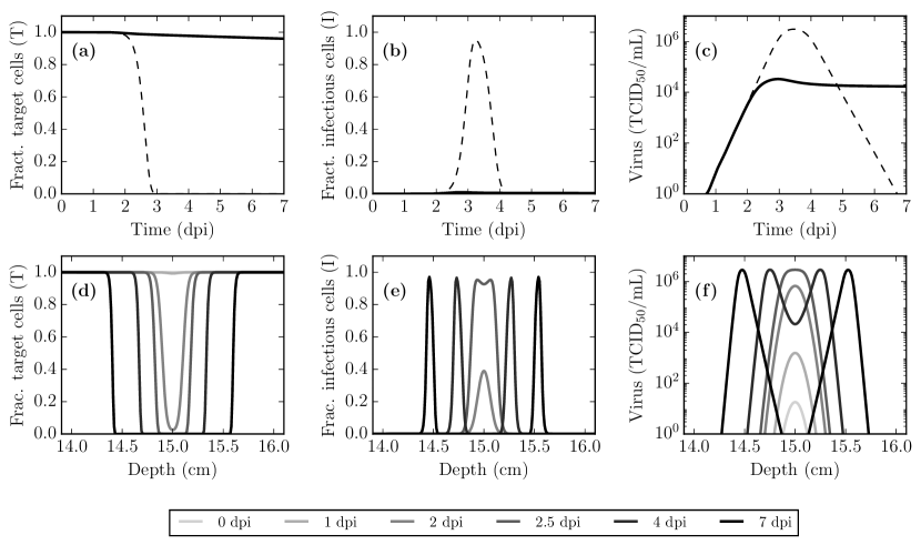
Figure 3(a–c) shows the IAV infection kinetics in the presence of both diffusion and upward advection as the virus production rate, , is increased from the base value estimated by Baccam et al. [1] for their non-spatial MM, (see Methods). Increasing the virus production rate to yields an infection that peaks at . This adjusted value for the virus production rate (, see Table 1) is used in the remainder of this work so that the spatial MM qualitatively reproduces the approximate timing of viral titer peak in an IAV infection.
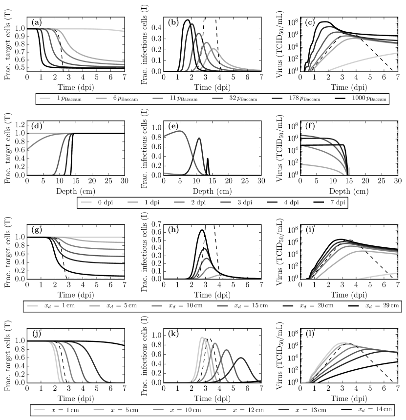
Using the new value for the virus production rate, Figure 3(d–f) shows the spatial extent of the infection dissemination in the presence of both diffusion and advection in the spatial MM. It illustrates the protective effect of advection: preventing the infection from travelling much beyond its initial deposition depth (), as seen from the target cell depletion shown in Figure 3(d). Figure 3(g–i) explores the effect of varying this depth of deposition of the initial virus inoculum, . When the inoculum deposits lower in the HRT (as increases), the fraction of HRT consumed by the infection increases, resulting in higher viral titer peak and total virus yield. However, the virus titer curve is largely insensitive to the depth of deposition for depths greater than .
In the presence of both diffusion and advection in the spatial MM, the initial virus inoculum travels quickly from its deposition site at a fixed speed up the HRT, leaving in its wake a small, equal fraction of infected cells at all sites above the deposition point (). As the newly infected cells begin to release virus which is entrained up the HRT, uninfected cells are only exposed to virus produced by cells lower than (upstream of) their own depth (greater value), such that cells higher in the HRT (smaller value) are exposed to the most virus. Consequently, infection in the upper HRT proceeds much faster than that in the lower HRT. Figure 3(j–l) shows the localized fraction of target and infectious cells, and infectious virus concentration over time at specific sites or depths along the HRT. Despite infection kinetic parameters being the same at all sites, infection progresses faster at sites located higher in the HRT, downstream of the virus flow.
Interestingly, the more rapid progression of the infection higher in the HRT makes it appear as though the infection is moving downwards, from the top (nose, ) towards the bottom () of the HRT. Both the target cell depletion wavefront in Figure 3(d) and the infected cell “pulse” in Figure 3(e) appear to be moving to the right (towards the lower HRT) as time advances. This can be seen more clearly in the video (S2 Video.) which depicts the spatiotemporal course of the infection, in the presence of both diffusion and advection. Cells in the upper HRT are consumed first, after which the pulse of infected cells appears to slowly move backwards, down the HRT, back to the initial deposition site, where it then slowly dissipates.
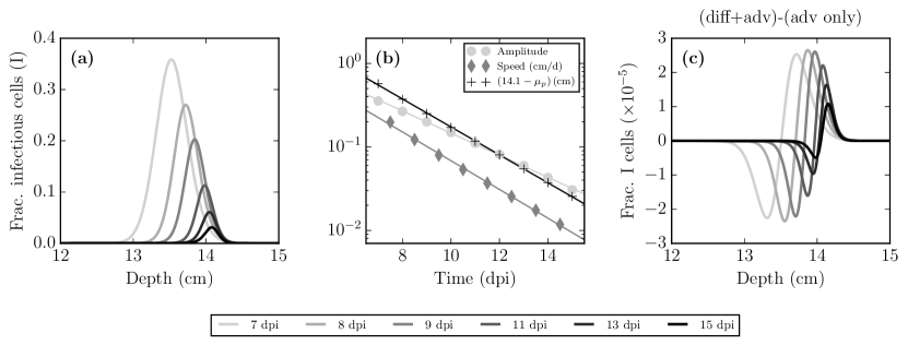
Figure 4(a) provides a more “zoomed-in” view of what happens to the pulse in Figure 3(e) at times beyond . The pulse is shrinking and slowing down as it approaches the initial inoculum deposition depth of . Figure 4(b) quantitatively displays the (nearly exponential) decay of both the amplitude and speed of the pulse, as its peak’s position () approaches its final, asymptotic position of , a little short of its initial deposition depth. Figure 4(c) shows the difference between the pulses obtained in the presence of both diffusion and advection minus that in the presence of advection alone (no diffusion). While advection dominates over diffusion, the latter still plays a role in allowing a small amount of virus to travel upstream, against the advection, which results in slightly more cells infected upstream and slightly less downstream. The effect of diffusion in the presence of advection is most likely negligible (one part in in the fraction of cells infected) in light of typical, in vivo experimental variability (10-fold variability).
2.3 Target cell regeneration during IAV infection
During an uncomplicated IAV infection, viral loads typically fall below detectable levels between – [13, 2]. An experimental study in which mice were sacrificed at various times over the course of an IAV infection [61] found that by , ciliated cells were rarely observed on the tracheal surface, and instead the latter was mostly composed of a layer of undifferentiated cells. By , signs of repair were apparent, by the tracheal surface was covered with ciliated and nonciliated cells, and by the surface was indistinguishable from the uninfected surface. Another experimental study in hamsters suggests that – after mechanical injury, most of the epithelium is comparable to that of control hamsters [42]. A similar study in guinea-pigs suggests that after mechanical injury, the epithelium was ciliated and differentiated, and by it was indistinguishable from that of control guinea-pigs [25]. Together, these studies suggest that the process of cellular regeneration following damage caused by an IAV infection would at least begin, if not be well underway, before the IAV infection has fully resolved.
Following airway injury, numerous factors are thought to trigger the start of the repair process [18]. Once triggered, it is believed neighbouring epithelial cells will try to stretch to cover the denuded area, and divide so as to regain their normal shape while maintaining coverage. As damage becomes more significant, progenitor cells, mainly basal cells exposed to the PCF as the epithelial cells above them detach or are removed by apoptosis or damage, also undergo proliferation and differentiation until the epithelium is restored to its pre-injury state [64]. With these processes in mind, cellular regeneration was implemented in the spatial MM by replacing the equation for uninfected, target cells in MM Eqn. (1) with
| (2) |
where
is the fraction of dead cells, i.e. the extent of the damage or injury. As such, cellular regeneration in Eqn. (2) proceeds at a rate that is greater in the presence of greater damage (higher ) and of greater fraction of cells available to regenerate (higher ). Parameter sets the scale of the regeneration rate (which also depends on and ), and is the regeneration delay such that the current regeneration rate depends on the fraction of target cells () currently available to repopulate the area, and on the amount of damage () that was perceived some time ago. The delay between damage and regeneration accounts for the time required for the damage to activate appropriate signalling pathways, and for both division and differentiation to take place so that newly regenerated cells are susceptible to infection. This same equation has been used by others to represent target cell regeneration during an IAV infection [28, 12], but the authors therein did not include a delay ().
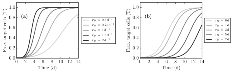
An experimental study of cell regeneration in hamsters [42] suggests that in many cases, between – following a mechanical injury, cells have already stretched or migrated to cover the complete denuded area and cell division has begun. A similar study in guinea-pigs [25] also suggests that at after mechanical injury, cells have migrated to cover the denuded area and cell proliferation is underway. This suggests that the delay between damage and the start of cellular division is around –. Herein, this delay — namely the time elapsed between damage and the start of both cellular division and differentiation to an extent that newly regenerated cells are susceptible to infection — was chosen to be , based on these experimental studies. To select an appropriate value for the regeneration rate (), HRT epithelial cell regeneration following mechanical injury was simulated using Eqn. (2). Results are shown in Figure 5 for different regeneration rates and delays: the regeneration rate determines the steepness of the regeneration, while the regeneration delay sets its timing. These parameters should be easily identifiable if experimental data was available. An intermediate value of was chosen to ensure that with a delay of , regeneration is well underway by –, and completely resolved by – [61, 25, 42].
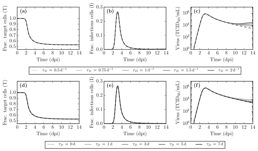
Figure 6 shows the infection kinetics in the presence of cellular regeneration. At this stage, and over the range of values considered here, the spatial MM is insensitive to the choice of regeneration rate or its delay. This is largely due to the fact that, in the absence of an immune response, the HRT above the inoculum deposition point is decimated by the infection at a rate much faster than the density-dependent regeneration can counter. As damage increases, the number of target cells available to replenish the lost cells also decreases dramatically, preventing any significant regeneration. To get a more realistic view of the role and impact of cellular regeneration on infection kinetics, the protective role of the immune response must be considered.
2.4 Immune response to an IAV infection
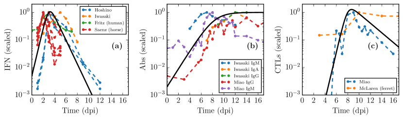
Past MM for IAV infection have incorporated one or more immune response components with varying degrees of success [23, 12, 11]. Difficulties in incorporating an immune response when modelling IAV infections include the complex nature of the interactions (large networks of cells and signals), and the lack of appropriate data (quantity and quality) to inform the MMs [29]. The simplified immune response considered herein comprises an innate response based on interferon (IFN), a humoral response represented by antibodies (Abs), and a cellular response embodied by cytotoxic T lymphocytes (CTLs). Since our aim is to display the MM’s range of kinetics — rather than identify parameters, analyze data, or challenge hypotheses — a parsimonious approach was preferred wherein key immune components are represented using empirical curves that broadly reproduce the scale and timing of these experimentally measured quantities (see Methods). Figure 7 shows the empirical MM curves against their corresponding experimental time courses, for IFN, Abs, and CTLs, during experimental, in vivo IAV infections.
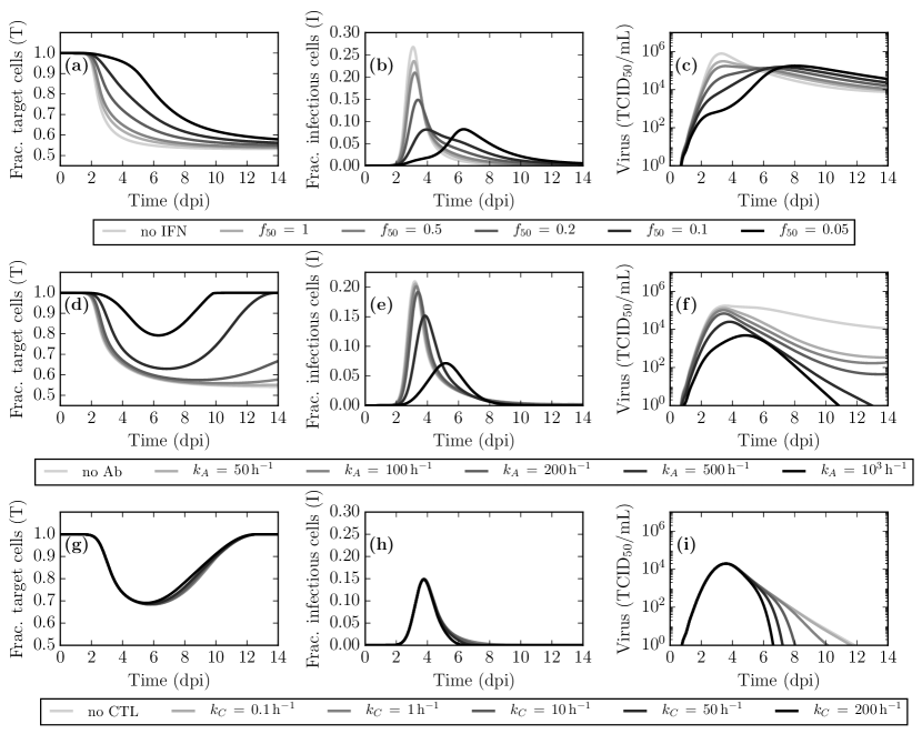
Although IFN is known to have many effects [40], herein its effect is to reduce the virus production rate [1, 30], via a resistance parameter, , analogous to the IC50 used to describe antiviral resistance. The resistance is defined such that if , the virus production rate is halved when IFN concentration is 80% of its peak value (see Methods). Figure 8(a–c) shows the effect of IFN in the MM as resistance to IFN, , is lowered (increased sensitivity). The initial viral titer peak is reduced due to IFN presence, with lower resistance (smaller ) having a greater impact. However, once IFN starts to decay, its effect rapidly dissipates, leading to a rise, or even a rebound, in the viral load. On its own, IFN does not lead to infection resolution in this MM.
The effect of Abs herein, like elsewhere [9, 28, 44, 30, 49], is to enhance infectious virus clearance such that becomes , where represents the neutralization rate of infectious virus by Abs, . Figure 8(d–f) shows the effect of IFN+Abs in the MM as the neutralization rate, , is increased. Low binding affinity Abs () cannot clear the infection. As increases, viral titer decay rates increase, leading to infection resolution within –. However, the time to infection resolution remains longer than the – typically observed for IAV infections in humans [13, 2].
The effect of CTLs herein, like elsewhere [9, 28, 44, 49], is to increase the rate of loss of infected cells expressing IAV peptides on their MHC-1. Infected cells begin expressing IAV peptides post-infection [9, 78], or approximately halfway through the eclipse phase ( in the spatial MM, see Table 1), such that all infected cells past the mid-point of their eclipse phase will be removed at rate , where represents the killing rate of infected cells by CTLs, . Figure 8(g–i) shows the effect of IFN+Abs+CTLs in the MM as the killing rate, , is increased. Higher CTL killing rates () cause the infection to resolve earlier.

Figure 9 shows the MM predictions and experimental data of immune response knockout experiments, wherein one component of the immune response is suppressed or neutralized. The MM prediction of an IFN knockout experiment is in good agreement with the experimental data of IFN knockout experiments [66, 38] at early time as both suggest IFN acts early and helps to reduce the initial viral titer peak. The experimental Ab knockout experiment [41] suggests Abs help reduce viral load at a later time in the infection but does not affect the initial viral titer peak. The MM prediction also suggests Abs help reduce the viral load at a later time but also affects the initial viral titer peak. This could be better reproduced by the MM by having a lower initial amount of Abs () so that Abs appear later and thus act later. Finally, the MM prediction of the CTL knockout experiment is in good agreement with the experimental data of CTL knockout experiments [81, 77, 43] as both suggest that CTLs act only at a late stage in the infection, helping reduce infection duration. Generally, the experimental knockout appear to show a greater impact for the knock-outs than predicted by the MM. This is likely due to the intricate interaction network between the different immune response components in vivo which makes it difficult to experimentally disrupt one component without affecting another.
2.5 Capturing the kinetics of in vivo infections with seasonal and avian IAV strains
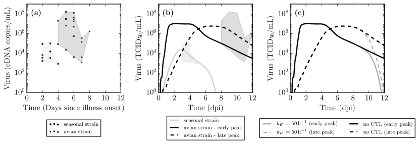
The difference in infection severity between patients naturally infected with seasonal IAV strain or avian-origin H5N1 strains is thought to be the result of a number of different possible factors, including more rapid infection and replication kinetics, cell tropism, lack of pre-existing immunity, and/or an aberrant immune response [19, 16, 14, 66, 67, 72, 74, 75, 39, 68]. Figure 10(a) shows viral load measurements from pharyngeal swabs of patients (each point is a single measure from a single patient) naturally infected with either a seasonal (H3N2 or H1N1) IAV strain or a strain of the H5N1 subtype. This study wherein these measures were taken over the same time period and following the same methodology, such that viral loads for infection with seasonal and H5N1 strains can be readily compared, is the only one of its kind. Since patients were recruited into the study days after illness onset, and began receiving antiviral therapy immediately upon hospital admission, untreated infection kinetics leading up to and after admission are not available. The measured pharyngeal viral load (determined via qRT-PCR) is 100-fold higher for patients infected with H5N1 than seasonal IAV strains. This could also be true of the infectious viral titer (typically measured via TCID50 or PFU) which was not measured as part of this study, although the ratio of infectious to total IAV is known to change over the course of an infection, and inconsistently so between experiments [58]. Another feature is that H5N1-infected patients reported to the hospital – later after illness onset than those infected with seasonal IAV strains. It is unclear whether this is due to a slower progression of infection with an H5N1 strain, or because patients infected with H5N1 strains mostly came from remote provinces and took longer to reach the city hospital than those infected with seasonal strains which came from the city itself or neighbouring provinces.
| IAV strain | IFN, | Abs∗, | CTLs, (h-1) | ||||
|---|---|---|---|---|---|---|---|
| seasonal | 50 | ||||||
| avian (early) | — | ||||||
| avian (late) | — |
* The rate of infectious virus neutralization by Abs was fixed to for all 3 infections.
From the data in Figure 10(a), two hypothetical infection time courses or portraits were developed for infection with IAV H5N1 strains, and one for seasonal strains, shown in Figure 10(b). The portrait for infection with a seasonal strain peaks at – at , and resolves by [34, 63]. For infection with a strain of the H5N1 subtype, two options are considered: the infection peaks early, at higher titers which are sustained over a longer period; or the infection grows at a rate similar to infection with a seasonal strain, but that growth is sustained over a longer period and thus peaks later, reaching higher titers than infection with a seasonal strain. For infection with an H5N1 strain, viral titer peak was chosen to be 100-fold higher, as observed for total viral loads, and the reported – delay in hospital admission was captured either as a longer, sustained infection in the early time course, or as a longer delay to reach peak titer in the late time course. The IAV H5N1 portraits were constructed from the MM of the seasonal portrait by shifting parameters controlling cell-virus interactions and immunity in keeping with differences believed to be responsible for that shift. These parameters are presented in Table 2. The shaded areas, which depict the extent of the data points in Figure 10(a) where time is based on days since illness onset, are shown time-shifted in Figure 10(b) where time is days post-infection. For a seasonal infection, the (pale grey) area was shifted to one day later since there is generally a delay of one day between infection and symptom onsets [13]. For avian infections, the (dark grey) area was shifted to 4 days later since reports suggest –5 days elapse between symptom onset and known potential exposure to infected poultry [35, 17, 53].
For cell-virus interactions, the early time course relies on increased virus production (), increased virus infectivity (), and a shorter eclipse phase (), consistent with shifts in these parameters estimated from in vitro infections of A549 cells with seasonal (H1N1) versus H5N1 and H7N9 IAV strains [68]. In contrast, the late time course relies on lower virus infectivity and a longer eclipse phase, along with a higher virus production rate. The early and late portraits also depend on 8- and 10-fold longer periods of virus production (infectious cell lifespan, ), respectively, compared to that for cells infected with a seasonal strain. In capturing differences in immunity, both the early and late portraits of infection with IAV H5N1 strains rely on 10-fold increased resistance to the effect of IFN (), decrease in pre-existing immunity in the form of a 200-fold decrease in the neutralizing effect of Abs, and the absence of a CTL response. The resistance of H5N1 strains to the effect of IFN- and - has been reported in vitro in porcine cell cultures and in vivo in pigs [66]. The decrease in the neutralizing efficacy of Abs is captured in the simplistic Ab MM utilized herein as a 200-fold decrease in their initial quantity () which means a longer time ( longer) to reach maximal Ab activity, but can equally be captured by a 200-fold decrease in the neutralization efficacy () of Abs. A recruitment study of patients naturally infected with avian H7N9 IAV strains reported that the patient group with the earliest recovery, had a prominent CTL response by post admission and a prominent Ab response, 2– later [76]. In contrast, the patient group with the most delayed recovery had an Ab and CTL response that remained low even after post admission. This suggests that an infection with an H5N1 strain, characterized by a prolonged viral shedding period, would have delayed Ab and CTL responses. Because the portraits in Figure 10(b) only go up to , the effect of these delayed CTLs would not be apparent. Figure 10(c) illustrates what the time course of infection with an avian strain could look like in the presence of a delayed CTL response, but one which would be as effective (same ) as that for infection with a seasonal strain. It shows an important role for CTLs in controlling the persistent shedding in these infections, consistent with the findings that a delayed CTL response correlated with slower recovery from infection with H7N9 strains [76].

| (\dpi) | [Resolution time (\dday)] | [AUC (\dday)] | [Viral titer peak()] |
|---|---|---|---|
| —Seasonal — | |||
| 2 | |||
| 3 | |||
| 6 | |||
| — Avian (early) — | |||
| 2 | |||
| 3 | |||
| 6 | |||
| — Avian (late) — | |||
| 2 | |||
| 3 | |||
| 6 | |||
∗ For NAI therapy administered at various times post infection (), the change () in 3 commonly reported endpoints are shown for the viral titer curves in Figure 11. The change in resolution time is computed as a difference (), whereas that for the area under the viral titer curve (AUC) and viral titer peak corresponds to the fold-change (). ND stands for not determined in cases where infection resolution () was not achieved without treatment.
Figure 11 explores the impact of antiviral therapy with neuraminidase inhibitors (NAIs), administered at various times post-infection, on the time courses for infection with seasonal or avian IAV strains. Since NAIs block the release of newly produced virions, their effect is implemented in the MM, as elsewhere [31, 20, 22, 8, 11, 21, 45, 54], as a reduction in the virus production rate, namely , from the time treatment is administered, where is the drug efficacy. The efficacy of NAIs was set to to study the case of treatment with a high efficacy. Table 3 quantitatively compares the impact of NAI treatment for various endpoints: reduction in resolution time, peak viral titer, and area under the viral titer curve (AUC).
Human volunteer studies in patients experimentally infected with seasonal (H1N1) IAV strains and treated with NAIs report that early treatment (24– post infection) is effective in reducing viral load [32, 33, 3], and one such study reports that delayed treatment ( post infection) is less effective [33], in line with the MM results. A study of H5N1-infected patients recruited days after illness onset, and beginning NAI treatment immediately after admission, reports that late treatment (4– after illness onset) is still effective in some patients, reducing viral load and thus possibly also reducing time to infection resolution. This would be consistent with some avian strain-infected patients experiencing an infection time course similar to the early portrait with moderate to no benefit from delayed NAI treatment, and others experiencing infection more consistent with the late portrait and benefiting from NAI therapy even when treatment initiation is delayed.
3 Discussion
Mathematical models (MMs) for the course of an influenza A virus (IAV) infection in vivo typically assume the infection is spatially homogeneous, i.e. that all cells see all virus, and vice-versa, instantly over all space. This simplification is reasonable in vitro in cell culture infections whose spatial extent is often no more than one or two square centimetres [37], but it is unclear whether it remains appropriate at the scale of the entire HRT. With simplicity and parsimony in mind, the spatial MM introduced herein represents the HRT as a one-dimensional track that extends from the nose down to a depth of . It implements two modes of viral transport: advection of virus upwards towards the nose, and diffusion of the virus within the periciliary fluid.
When diffusion alone is considered, infection in the spatial MM proceeds at a slower pace than in the non-spatial MM, but virus production is sustained for longer. The diffusion initially acts to spatially restrict the number of cells available to the infection, and then releases these cells progressively as the diffusing infection wave reaches ever further in the HRT. When advection is added to diffusion, the former dominates the infection kinetics, requiring a 10-fold increase in the virus production rate to restore the timing and level of viral titer peak to that in the non-spatial MM. This is noteworthy, firstly, because it shows that advection constitutes an effective physiological mechanism to suppress infection. Secondly, it shows that use of a non-spatial MM to analyze infection data possibly underestimates the virus production rate, and consequently also the total amount of virus produced over the course of an infection. Since the more virus are produced, the more mutations accumulate [24, 57, 31], underestimating the virus production rate means underestimating the rate and likelihood of emergence of drug resistance.
Interestingly, the MM suggests that the depth at which the initial virus inoculum deposits also plays a major role in determining the extent of HRT involvement in the infection. Specifically, the MM predicts no target cell consumption below the depth at which the initial virus inoculum deposits. While deposition at depths lower than did not affect the viral titer time course, initial depositions above that point both delayed and reduced peak titer. As such, higher virus production rates would be required to compensate for shallower deposition depths to obtain equivalent viral titer time courses. This is one more way a non-spatial MM might underestimate the rate of virus production, and thus the likelihood of antiviral resistance emergence.
A more unexpected finding was that although kinetically in the spatial MM the infection deposits at some depth and is dragged upwards by advection, the infection appears to be moving from the upper to the lower HRT. This is because the upper HRT is downstream of virus advection and sees most of the virus produced, while the lower HRT is upstream and sees little or none. Therefore, infection progresses, peaks and resolves faster in the upper HRT and slower in the lower HRT. It is this difference in time scale which makes it appear as though the infection is moving from the upper to the lower HRT. Experimental studies of mice infected with IAVs engineered to be fluorescent or bioluminescent observe infection spread from the upper towards the lower regions of the lung [46, 73], consistent with the MM’s predictions. In the absence of sufficient immune control, this could serve to maintain the infection with, wherein the slower, lower HRT infection could re-ignite more rounds of infection in the upper HRT, depending on the delicate timing between infection time course in the lower HRT and cell regeneration in the upper HRT.
The spatial MM was expanded to include density-dependent cell regeneration, and a simplistic immune response comprising IFN acting to down-regulate the rate of virus production by infected cells, Abs neutralizing infectious virions, and CTLs killing infected cells. In the presence of this immune response, the MM-simulated IAV infection was well controlled and resolved fully by . The spatial MM could also largely reproduce the key features of in vivo immune response knockout experiments [23]. In the MM-simulated infection (see Figure 8g), 10% of the HRT was involved in the infection by , around the fraction of cells involved in the infection peaked at 30%, and by 10% of the epithelium had yet to regenerate, although viral titers had fallen below the detection limit (see Figure 8i). These numbers align well with a 1989 report in Russian cited by Bocharov and Romanyukha in their 1994 IAV MM paper [9] of 10% damage at symptom onset, 30–50% of the upper airway destroyed at the peak of the disease, and resolution of disease at a time when as much as 10% of the normal epithelium is still damaged.
The full spatial MM was applied to simulate the kinetics of infection with either a mild, seasonal IAV strain or a severe infection with an avian strain such as H5N1. Since complete, untreated, infection kinetic time courses for infection with avian IAV strains are not available, two different portraits were constructed to represent plausible time courses: one peaking early with sustained, high titers over several days, and another rising slowly, similarly to seasonal infections, but continuing on to reach high titers 3–4 days later. Differences in the time courses for infection with a seasonal vs avian IAV strain could be captured by the MM by shifting the parameters in ways that are consistent with known or expected differences between infections with seasonal and avian strains. The portraits were used to evaluate the impact of antiviral therapy with neuraminidase inhibitors. Treatment was most effective for the seasonal and late peak avian IAV strain portraits when administered early during the infection at . Later treatment was of limited effectiveness for the seasonal IAV strain portrait, but was still effective in the late peaking portrait of infection with an avian IAV strain.
The spatial MM presented herein, despite its simplicity, offers a novel and interesting opportunity to study the spatial localization and dissemination of IAV infections within the HRT. In the future, the addition of an explicit, dynamical immune response — to replace the empirical equations used herein as stand-ins for immune response components — would enable the use of this MM to reproduce the kinetics of re-infection, similar to the work done by others [12, 79].
4 Supporting information
S1 Video.
Spatiotemporal course of IAV infection in the presence of diffusion only (no advection).
S2 Video.
Spatiotemporal course of IAV infection in the presence of diffusion and advection.
5 Acknowledgements
This work was supported in part by Discovery Grant 355837-2013 (to CAAB) from the Natural Sciences and Engineering Research Council of Canada (www.nserc-crsng.gc.ca), Early Researcher Award ER13-09-040 (to CAAB) from the Ministry of Research and Innovation of the Government of Ontario (www.ontario.ca/page/early-researcher-awards), and by Interdisciplinary Theoretical and Mathematical Sciences (iTHEMS, ithems.riken.jp) at RIKEN (CAAB).
6 Financial disclosures
CAAB received financial support in the form of a research contract and a consultancy fee from F. Hoffmann-La Roche Ltd. in the early stages of this project. MBR was employed by F. Hoffmann-La Roche Ltd. when first participating in this work, and is currently employed by Array BioPharma Inc.. Neither company had any role in the study design, data collection and analysis, or decision to publish.
7 Methods
7.1 Numerical implementation of the mathematical model
The Euler method was used to numerically solve the cell population equations, namely
| (3) | ||||
where , , , and and are the chosen spatial and temporal step sizes, respectively. We define , the number of spatial boxes or sites that make up the simulated HRT such that , the diameter of 4–5 epithelial cells. This was chosen by verifying that choosing a larger number of sites (smaller ) did not affect the solution. When presenting the fraction of target cells or infectious cells, or the virus concentration, as a function of time only, averaged over space, those are computed as
For the virus concentration, for simplicity, the diffusion and advection terms are each treated separately, and are applied before the production and clearance terms are considered. To solve the diffusion term, the Crank-Nicolson method was used, namely
where . The rate of viral diffusion in the PCF was estimated based on the Stokes-Einstein equation for IAV diffusing in plasma at body temperature as [37, 6]. An absorbing boundary condition was used at the top of the HRT, (or ), to capture virus flow out through the mouth and nose. A reflective boundary condition, (or ), was used at the bottom of the HRT. The bottom boundary condition becomes irrelevant once advection is introduced as the flow at becomes negligible. With these boundary conditions in place, the diffusion of virus over a step size can be expressed as
The virus advection term can be written as follows
| (4) | ||||
This simplistic numerical scheme is known to lead to a dispersion (diffusion) of the solution [52]. However, the spatial MM simulator imposes , such that Eqn. (4) simplifies to , a trivial translation of the solution, which ensures the latter will remain stable and will not disperse. The speed of the PCF is believed to be approximately the same as that of the mucus blanket and is estimated to be [47]. This requires the time step for the spatial MM simulator to be . Here, the boundary condition at the top is irrelevant since the solution depends only on the downstream element (), and the boundary condition at the bottom is chosen such that , i.e. there is no virus beyond the end of the HRT. Once diffusion and advection have been applied, the Euler method is used to solve the remaining terms of the virus equation, namely
| (5) |
The droplet-like, initial IAV distribution is represented by a Gaussian centred at the site of deposition,
| (6) |
where is the site of deposition, , and is chosen so that , i.e. the spatial average of the initial virus inoculum concentration in the spatial MM herein is equal to in the non-spatial ODE MM by Baccam et al. [1].
While most parameters were taken directly from [1], some were adapted. Whereas in Baccam et al. [1] corresponds to the number of cells, in the spatial MM herein, fraction of cells in each state are considered instead such that . As such, what we consider the Baccam et al. [1] virus production rate is converted from that reported in their paper as
Once advection is introduced (see Results), a value of is used so that the virus titer will peak at roughly 2–, consistent with that observed in Baccam et al. [1].
7.2 Empirical, mathematical representation of the immune response
The time course for interferon (IFN) is represented as
| (7) |
where and are the growth and decay rates of IFN respectively, and is the time of peak. Since , represents the fractional amount of IFN, relative to peak IFN, at time . In the MM, , and to match experimental data. Its effect in the MM is to attenuate virus production, , captured as
| (8) |
where is the amount of IFN required to reduce the virus production rate to one half its normal value, i.e. when . In the MM, is normalized so as to have a maximum value of (). As such, if , then when .
The time course of antibodies (Abs) is represented as
| (9) |
where is the initial amount of Abs, and is the growth rate of Abs. Since , represents the fractional amount of Abs, relative to peak Abs, at time . In the MM, and to match experimental data. The effect of Abs in the MM is to enhance virus clearance, , captured as
| (10) |
where represents the binding affinity of Abs.
The time course of cytotoxic T lymphocytes (CTLs) is represented as
| (11) |
where and are the growth and decay rates of CTLs, respectively, and is the time of peak. Since , represents the fractional amount of CTLs, relative to peak CTLs, at time . In the MM, , and to match experimental data. The effect of CTLs in the MM is to increase the rate of loss of IAV-infected cells which CTLs recognize as infected. Newly infected cells begin to present IAV peptides on their MHC-1 for CTL recognition after IAV infection [9, 78]. In our MM, this corresponds approximately to half the duration of the eclipse phase (): cells in would not be presenting peptides, while those in would be recognizable and thus could be killed by CTLs. As such, killing of recognizably-infected cells by CTLs in the MM is captured as
| (12) | ||||||
where provides the scale for the rate of infected cell killing by CTLs.
References
- [1] P. Baccam, C. Beauchemin, C. A. Macken, F. G. Hayden, and A. S. Perelson. Kinetics of influenza A virus infection in humans. J. Virol., 80(15):7590–7599, 2 August 2006. doi:10.1128/JVI.01623-05.
- [2] S. Balasingam and A. Wilder-Smith. Randomized controlled trials for influenza drugs and vaccines: A review of controlled human infection studies. Int. J. Infect. Dis., 49:18–29, August 2016. doi:10.1016/j.ijid.2016.05.013.
- [3] L. Barroso, J. Treanor, L. Gubareva, and F. G. Hayden. Efficacy and tolerability of the oral neuraminidase inhibitor peramivir in experimental human influenza: Randomized, controlled trials for prophylaxis and treatment. Antivir. Ther., 10(8):901–910, 2005.
- [4] A. L. Bauer, C. A. A. Beauchemin, and A. S. Perelson. Agent-based modeling of host-pathogen systems: The successes and challenges. Inform. Sciences, 179(10):1379–1389, 29 April 2009. doi:10.1016/j.ins.2008.11.012.
- [5] C. Beauchemin. Probing the effects of the well-mixed assumption on viral infection dynamics. J. Theor. Biol., 242(2):464–477, 21 September 2006. doi:10.1016/j.jtbi.2006.03.014.
- [6] C. Beauchemin, S. Forrest, and F. T. Koster. Modeling influenza viral dynamics in tissue. In H. Bersini and J. Carneiro, editors, Proceedings of the International Conference on Artificial Immune Systems (ICARIS 06), number 4163 in Lecture Notes in Computer Science, pages 23–36. Springer-Verlag Berlin Heidelberg, 2006. doi:10.1007/11823940_3.
- [7] C. Beauchemin, J. Samuel, and J. Tuszynski. A simple cellular automaton model for influenza A viral infections. J. Theor. Biol., 232(2):223–234, 21 January 2005. doi:10.1016/j.jtbi.2004.08.001.
- [8] N. F. Beggs and H. M. Dobrovolny. Determining drug efficacy parameters for mathematical models of influenza. J. Biol. Dyn., 9(sup1):332–346, 9 June 2015. doi:10.1080/17513758.2015.1052764.
- [9] G. A. Bocharov and A. A. Romanyukha. Mathematical model of antiviral immune response III. Influenza A virus infection. J. Theor. Biol., 167(4):323–360, 21 April 1994. doi:10.1006/jtbi.1994.1074.
- [10] A. Boianelli, V. K. Nguyen, T. Ebensen, K. Schulze, E. Wilk, N. Sharma, S. Stegemann-Koniszewski, D. Bruder, F. R. Toapanta, C. A. Guzmán, M. Meyer-Hermann, and E. A. Hernandez-Vargas. Modeling influenza virus infection: A roadmap for influenza research. Viruses, 7(10):5274–5304, 12 October 2015. doi:10.3390/v7102875.
- [11] P. Cao and J. M. McCaw. The mechanisms for within-host influenza virus control affect model-based assessment and prediction of antiviral treatment. Viruses, 9(8):E197, 26 July 2017. doi:10.3390/v9080197.
- [12] P. Cao, A. W. Yan, J. M. Heffernan, S. Petrie, R. G. Moss, L. A. Carolan, T. A. Guarnaccia, A. Kelso, I. G. Barr, J. McVernon, K. L. Laurie, and J. M. McCaw. Innate immunity and the inter-exposure interval determine the dynamics of secondary influenza virus infection and explain observed viral hierarchies. PLoS Comput. Biol., 11(8):e1004334, 18 August 2015. doi:10.1371/journal.pcbi.1004334.
- [13] F. Carrat, E. Vergu, N. M. Ferguson, M. Lemaitre, S. Cauchemez, S. Leach, and A.-J. Valleron. Time lines of infection and disease in human influenza: A review of volunteer challenge studies. Am. J. Epidemiol., 167(7):775–785, 1 April 2008. doi:10.1093/aje/kwm375.
- [14] M. Chan, C. Cheung, W. Chui, S. Tsao, J. Nicholls, Y. Chan, R. Chan, H. Long, L. Poon, Y. Guan, and J. Peiris. Proinflammatory cytokine responses induced by influenza A (H5N1) viruses in primary human alveolar and bronchial epithelial cells. Respir. Res., 6(1):135, 11 November 2005. doi:10.1186/1465-9921-6-135.
- [15] M. C. Chan, R. W. Chan, W. C. Yu, C. C. Ho, W. Chiu, C. Lo, K. M. Yuen, Y. Guan, J. M. Nicholls, and J. M. Peiris. Influenza H5N1 virus infection of polarized human alveolar epithelial cells and lung microvascular endothelial cells. Respir. Res., 10(1), 30 October 2009. doi:10.1186/1465-9921-10-102.
- [16] C. Y. Cheung, L. L. M. Poon, A. S. Lau, W. Luk, Y. L. Lau, K. F. Shortridge, S. Gordon, Y. Guan, and J. S. M. Peiris. Induction of proinflammatory cytokines in human macrophages by influenza A (H5N1) viruses: A mechanism for the unusual severity of human disease? Lancet, 360(9348):1831–1837, 7 December 2002. doi:10.1016/s0140-6736(02)11772-7.
- [17] T. Chotpitayasunondh, K. Ungchusak, W. Hanshaoworakul, S. Chunsuthiwat, P. Sawanpanyalert, R. Kijphati, S. Lochindarat, P. Srisan, P. Suwan, Y. Osotthanakorn, T. Anantasetagoon, S. Kanjanawasri, S. Tanupattarachai, J. Weerakul, R. Chaiwirattana, M. Maneerattanaporn, R. Poolsavatkitikool, K. Chokephaibulkit, A. Apisaranthanarak, and S. F. Dowell. Human disease from influenza A (H5N1), Thailand, 2004. Emerg. infect. Dis., 11(2):201–209, February 2005. doi:10.3201/eid1102.041061.
- [18] L. M. Crosby and C. M. Waters. Epithelial repair mechanisms in the lung. Am. J. Physiol. Lung Cell Mol. Physiol., 298(6):L715–L731, June 2010. doi:10.1152/ajplung.00361.2009.
- [19] M. D. de Jong, C. P. Simmons, T. T. Thanh, V. M. Hien, G. J. D. Smith, T. N. B. Chau, D. M. Hoang, N. V. V. Chau, T. H. Khanh, V. C. Dong, P. T. Qui, B. V. Cam, D. Q. Ha, Y. Guan, J. S. M. Peiris, N. T. Chinh, T. T. Hien, and J. Farrar. Fatal outcome of human influenza A (H5N1) is associated with high viral load and hypercytokinemia. Nat. Med., 12(10):1203–1207, October 2006. doi:10.1038/nm1477.
- [20] H. M. Dobrovolny, M. J. Baron, R. Gieschke, B. E. Davies, N. L. Jumbe, and C. A. A. Beauchemin. Exploring cell tropism as a possible contributor to influenza infection severity. PLoS One, 5(11):e13811, 23 November 2010. doi:10.1371/journal.pone.0013811.
- [21] H. M. Dobrovolny and C. A. A. Beauchemin. Modelling the emergence of influenza drug resistance: The roles of surface proteins, the immune response and antiviral mechanisms. PLoS One, 12(7):e0180582, 10 July 2017. doi:10.1371/journal.pone.0180582.
- [22] H. M. Dobrovolny, R. Gieschke, B. E. Davies, N. L. Jumbe, and C. A. A. Beauchemin. Neuraminidase inhibitors for treatment of human and avian strain influenza: A comparative study. J. Theor. Biol., 269(1):234–244, 21 January 2011. doi:10.1016/j.jtbi.2010.10.017.
- [23] H. M. Dobrovolny, M. B. Reddy, M. A. Kamel, C. R. Rayner, and C. A. A. Beauchemin. Assessing mathematical models of influenza infections using features of the immune response. PLoS One, 8(2):e57088, 28 February 2013. doi:10.1371/journal.pone.0057088.
- [24] J. W. Drake. Rates of spontaneous mutation among RNA viruses. Proc. Natl. Acad. Sci. U.S.A., 90(9):4171–4175, 1 May 1993. doi:10.1073/pnas.90.9.4171.
- [25] J. S. Erjefält, I. Erjefält, F. Sundler, and C. G. A. Persson. In vivo restitution of airway epithelium. Cell Tissue Res., 281(2):305–316, August 1995. doi:10.1007/bf00583399.
- [26] J. V. Fahy and B. F. Dickey. Airway mucus function and dysfunction. N. Engl. J. Med., 363(23):2233–2247, 2 December 2010. doi:10.1056/NEJMra0910061.
- [27] R. S. Fritz, F. G. Hayden, D. P. Calfee, L. M. R. Cass, A. W. Peng, W. G. Alvord, W. Strober, and S. E. Straus. Nasal cytokine and chemokine response in experimental influenza A virus infection: Results of a placebo-controlled trial of intravenous zanamivir treatment. J. Infect. Dis., 180(3):586–593, September 1999. doi:10.1086/314938.
- [28] B. Hancioglu, D. Swigon, and G. Clermont. A dynamical model of human immune response to influenza A virus infection. J. Theor. Biol., 246(1):70–86, 7 May 2010. doi:10.1016/j.jtbi.2006.12.015.
- [29] A. Handel, L. E. Liao, and C. A. A. Beauchemin. Progress and trends in mathematical modelling of influenza A virus infections. Curr. Opin. Syst. Biol., 12:30–36, December 2018. doi:10.1016/j.coisb.2018.08.009.
- [30] A. Handel, I. M. Longini, and R. Antia. Towards a quantitative understanding of the within-host dynamics of influenza A infections. J R Soc Interface., 7(42):35–47, 6 January 2010. doi:10.1098/rsif.2009.0067.
- [31] A. Handel, I. M. Longini, Jr., and R. Antia. Neuraminidase inhibitor resistance in influenza: Assessing the danger of its generation and spread. PLoS Comput. Biol., 3(12):e240, December 2007. doi:10.1371/journal.pcbi.0030240.
- [32] F. G. Hayden, J. J. Treanor, R. F. Betts, M. Lobo, J. D. Esinhart, and E. K. Hussey. Safety and efficacy of the neuraminidase inhibitor GG167 in experimental human influenza. JAMA., 275(4):295–299, January 1996.
- [33] F. G. Hayden, J. J. Treanor, R. S. Fritz, M. Lobo, R. F. Betts, M. Miller, N. Kinnersley, R. G. Mills, P. Ward, and S. E. Straus. Use of the oral neuraminidase inhibitor oseltamivir in experimental human influenza: Randomized controlled trials for prevention and treatment. JAMA., 282(13):1240–1246, 6 October 1999. doi:10.1001/jama.282.13.1240.
- [34] F. G. Hayden, A. R. Tunkel, J. J. Treanor, R. F. Betts, S. Allerheiligen, and J. Harris. Oral LY217896 for prevention of experimental influenza A virus infection and illness in humans. Antimicrob. Agents Chemother., 38(5):1178–1181, May 1994. doi:10.1128/aac.38.5.1178.
- [35] T. T. Hien, N. T. Liem, N. T. Dung, L. T. San, P. P. Mai, N. van Vinh Chau, P. T. Suu, V. C. Dong, L. T. Q. Mai, N. T. Thi, D. B. Khoa, L. P. Phat, N. T. Truong, H. T. Long, C. V. Tung, L. T. Giang, N. D. Tho, L. H. Nga, N. T. K. Tien, L. H. San, L. V. Tuan, C. Dolecek, T. T. Thanh, M. de Jong, C. Schultsz, P. Cheng, W. Lim, and P. Horby. Avian influenza A (H5N1) in 10 patients in Vietnam. N. Eng. J. Med., 350(12):1179–1188, 18 March 2004. doi:10.1056/NEJMoa040419.
- [36] B. P. Holder and C. A. A. Beauchemin. Exploring the effect of biological delays in kinetic models of influenza within a host or cell culture. BMC Public Health, 11(Suppl 1):S10, 25 February 2011. doi:10.1186/1471-2458-11-S1-S10.
- [37] B. P. Holder, L. E. Liao, P. Simon, G. Boivin, and C. A. A. Beauchemin. Design considerations in building in silico equivalents of common experimental influenza virus assays. Autoimmunity, 44(4), June 2011. doi:10.3109/08916934.2011.523267.
- [38] A. Hoshino, H. Takenaka, O. Mizukoshi, J. Imanishi, T. Kishida, and M. G. Tovey. Effect of anti-interferon serum of influenza virus infection in mice. Antiviral Res., 3(1):59–65, March 1983.
- [39] S.-M. Hsieh and S.-C. Chang. Insufficient perforin expression in CD8+ T cells in response to hemagglutinin from avian influenza (H5N1) virus. J. Immunol., 176(8):4530–4533, 15 April 2006. doi:10.4049/jimmunol.176.8.4530.
- [40] A. Iwasaki and P. S. Pillai. Innate immunity to influenza virus infection. Nat. Rev. Immunol., 14(5):315–328, May 2014. doi:10.1038/nri3665.
- [41] T. Iwasaki and T. Nozima. Defense mechanisms against primary influenza virus infection in mice. I. The roles of interferon and neutralizing antibodies and thymus dependence of interferon and antibody production. J. Immunol, 118(1):256–263, January 1977.
- [42] K. P. Keenan, T. S. Wilson, and E. M. McDowell. Regeneration of hamster tracheal epithelium after mechanical injury. Virchows Arch. B Cell Pathol. Incl. Mol. Pathol., 43(3):213–240, 1983.
- [43] R. M. Kris, R. A. Yetter, R. Cogliano, R. Ramphal, and P. A. Small. Passive serum antibody causes temporary recovery from influenza virus infection of the nose, trachea and lung of nude mice. Immunology, 63(3):349–353, March 1988.
- [44] H. Y. Lee, D. J. Topham, S. Y. Park, J. Hollenbaugh, J. Treanor, T. R. Mosmann, X. Jin, B. M. Ward, H. Miao, J. Holden-Wiltse, A. S. Perelson, M. Zand, and H. Wu. Simulation and prediction of the adaptive immune response to influenza A virus infection. J. Virol., 83(14):7151–7165, July 2009. doi:10.1128/JVI.00098-09.
- [45] L. E. Liao, S. Kowal, D. A. Cardenas, and C. A. A. Beauchemin. Exploring virus release as a bottleneck for the spread of influenza A virus infection in vitro and the implications for antiviral therapy with neuraminidase inhibitors. PLoS One, 12(8):e0183621, 24 August 2017. doi:10.1371/journal.pone.0183621.
- [46] B. Manicassamy, S. Manicassamy, A. Belicha-Villanueva, G. Pisanelli, B. Pulendran, and A. García-Sastre. Analysis of in vivo dynamics of influenza virus infection in mice using a GFP reporter virus. Proc. Natl. Acad. Sci. U.S.A., 107(25):11531–11536, 22 June 2010. doi:10.1073/pnas.0914994107.
- [47] H. Matsui, S. H. Randell, S. W. Peretti, C. W. Davis, and R. C. Boucher. Coordinated clearance of periciliary liquid and mucus from airway surfaces. J. Clin. Invest., 102(6):1125–1131, 15 September 1998. doi:10.1172/JCI2687.
- [48] C. McLaren and G. M. Butchko. Regional T- and B-cell responses in influenza-infected ferrets. Infect. Immun., 22(1):189–194, October 1978.
- [49] H. Miao, J. A. Hollenbaugh, M. S. Zand, J. Holden-Wiltse, T. R. Mosmann, A. S. Perelson, H. Wu, and D. J. Topham. Quantifying the early immune response and adaptive immune response kinetics in mice infected with influenza A virus. J. Virol., 84(13):6687–6698, July 2010. doi:10.1128/JVI.00266-10.
- [50] H. Mitchell, D. Levin, S. Forrest, C. A. A. Beauchemin, J. Tipper, J. Knight, N. Donart, R. C. Layton, J. Pyles, P. Gao, K. S. Harrod, A. S. Perelson, and F. Koster. Higher level of replication efficiency of 2009 (H1N1) pandemic influenza virus than those of seasonal and avian strains: Kinetics from epithelial cell culture and computational modeling. J. Virol., 85(2):1125–1135, January 2011. doi:10.1128/JVI.01722-10.
- [51] R. Mora, E. Rodriguez-Boulan, P. Palese, and A. García-Sastre. Apical budding of a recombinant influenza A virus expressing a hemagglutinin protein with a basolateral localization signal. J. Virol., 76(7):3544–3553, April 2002. doi:10.1128/jvi.76.7.3544-3553.2002.
- [52] K. W. Morton and D. F. Mayers. Numerical solution of partial differential equations: An introduction. Cambridge University Press, Cambridge, UK, 2nd edition, 11 April 2005.
- [53] A. F. Oner, A. Bay, S. Arslan, H. Akdeniz, H. A. Sahin, Y. Cesur, S. Epcacan, N. Yilmaz, I. Deger, B. Kizilyildiz, H. Karsen, and M. Ceyhan. Avian influenza A (H5N1) infection in eastern Turkey in 2006. N. Engl. J. Med., 355(21):2179–2185, 23 November 2006. doi:10.1056/NEJMoa060601.
- [54] J. Palmer, H. M. Dobrovolny, and C. A. A. Beauchemin. The in vivo efficacy of neuraminidase inhibitors cannot be determined from the decay rates of influenza viral titers observed in treated patients. Sci. Rep., 7:40210, 9 January 2017. doi:10.1038/srep40210.
- [55] E. G. Paradis, L. T. Pinilla, B. P. Holder, Y. Abed, G. Boivin, and C. A. A. Beauchemin. Impact of the H275Y and I223V mutations in the neuraminidase of the 2009 pandemic influenza virus in vitro and evaluating experimental reproducibility. PLoS One, 10(5):e0126115, 20 May 2015. doi:10.1371/journal.pone.0126115.
- [56] J. S. M. Peiris, M. D. de Jong, and Y. Guan. Avian influenza virus (H5N1): A threat to human health. Clin. Microbiol. Rev., 20(2):243–267, April 2007. doi:10.1128/CMR.00037-06.
- [57] A. S. Perelson, L. Rong, and F. G. Hayden. Combination antiviral therapy for influenza: Predictions from modeling of human infections. J Infect Dis., 205(11):1642–1645, June 2012. doi:10.1093/infdis/jis265.
- [58] S. M. Petrie, T. Guarnaccia, K. L. Laurie, A. C. Hurt, J. McVernon, and J. M. McCaw. Reducing uncertainty in within-host parameter estimates of influenza infection by measuring both infectious and total viral load. PLoS One, 8(5):e64098, 15 May 2013. doi:10.1371/journal.pone.0064098.
- [59] L. T. Pinilla, B. P. Holder, Y. Abed, G. Boivin, and C. A. A. Beauchemin. The H275Y neuraminidase mutation of the pandemic A/H1N1 virus lengthens the eclipse phase and reduces viral output of infected cells, potentially compromising fitness in ferrets. J. Virol., 86(19):10651–10660, October 2012. doi:10.1128/JVI.07244-11.
- [60] O. G. Raabe, H. C. Yeh, G. M. Schum, and R. F. Phalen. Tracheobronchial geometry: Human, dog, rat, hamster. Report, Lovelace Foundation, 1976.
- [61] R. Ramphal, W. Fischlschweiger, J. W. Shands, Jr., and P. A. Small, Jr. Murine influenzal tracheitis: A model for the study of influenza and tracheal epithelial repair. Am. Rev. Respir. Dis., 120(6):1313–1324, December 1979. doi:10.1164/arrd.1979.120.6.1313.
- [62] L. A. Reperant, T. Kuiken, B. T. Grenfell, A. D. M. E. Osterhaus, and A. P. Dobson. Linking influenza virus tissue tropism to population-level reproductive fitness. PLoS One, 7(8):e43115, 28 August 2012. doi:10.1371/journal.pone.0043115.
- [63] P. D. Reuman, D. I. Bernstein, M. C. Keefer, E. C. Young, J. R. Sherwood, and G. M. Schiff. Efficacy and safety of low dosage amantadine hydrochloride as prophylaxis for influenza A. Antivir. Res., 11(1):27–40, February 1989.
- [64] J. R. Rock, M. W. Onaitis, E. L. Rawlins, Y. Lu, C. P. Clark, Y. Xue, S. H. Randell, and B. L. M. Hogan. Basal cells as stem cells of the mouse trachea and human airway epithelium. Proc. Natl. Acad. Sci. U.S.A., 106(31):12771–12775, 4 August 2009. doi:10.1073/pnas.0906850106.
- [65] R. A. Saenz, M. Quinlivan, D. Elton, S. MacRae, A. S. Blunden, J. A. Mumford, J. M. Daly, P. Digard, A. Cullinane, B. T. Grenfell, J. W. McCauley, J. L. N. Wood, and J. R. Gog. Dynamics of influenza virus infection and pathology. J. Virol., 84(8):3974–3983, April 2010. doi:10.1128/JVI.02078-09.
- [66] S. H. Seo, E. Hoffmann, and R. G. Webster. Lethal H5N1 influenza viruses escape host anti-viral cytokine responses. Nat, Med., 8(9):950–954, September 2002. doi:10.1038/nm757.
- [67] K. Shinya, M. Ebina, S. Yamada, M. Ono, N. Kasai, and Y. Kawaoka. Avian flu: Influenza virus receptors in the human airway. Nature, 440(7083):435–436, 23 March 2006. doi:10.1038/440435a.
- [68] P. F. Simon, M.-A. de La Vega, E. Paradis, E. Mendoza, K. M. Coombs, D. Kobasa, and C. A. A. Beauchemin. Avian influenza viruses that cause highly virulent infections in humans exhibit distinct replicative properties in contrast to human H1N1 viruses. Sci. Rep., 6:24154, 15 April 2016. doi:10.1038/srep24154.
- [69] D. J. Smith, E. A. Gaffney, and J. R. Blake. Modelling mucociliary clearance. Respir. Physiol. Neurobiol., 163(1–3):178–188, 30 November 2008. doi:10.1016/j.resp.2008.03.006.
- [70] M. D. Stoneham. The nasopharyngeal airway. Assessment of position by fibreoptic laryngoscopy. Anaesthesia, 48(7):575–580, July 1993. doi:10.1111/j.1365-2044.1993.tb07119.x.
- [71] M. C. Strain, D. D. Richman, J. K. Wong, and H. Levine. Spatiotemporal dynamics of HIV propagation. J. Theor. Biol., 218(1):85–96, 7 September 2002. doi:10.1006/jtbi.2002.3055.
- [72] C. I. Thompson, W. S. Barclay, M. C. Zambon, and R. J. Pickles. Infection of human airway epithelium by human and avian strains of influenza A virus. J. Virol., 80(16):8060–8068, August 2006. doi:10.1128/JVI.00384-06.
- [73] V. Tran, L. A. Moser, D. S. Poole, and A. Mehle. Highly sensitive real-time in vivo imaging of an influenza reporter virus reveals dynamics of replication and spread. J. Virol., 87(24):13321–13329, December 2013. doi:10.1128/JVI.02381-13.
- [74] D. van Riel, V. J. Munster, E. de Wit, G. F. Rimmelzwaan, R. A. M. Fouchier, A. D. M. E. Osterhaus, and T. Kuiken. H5N1 virus attachment to lower respiratory tract. Science, 312(5772):399, 21 April 2006.
- [75] D. van Riel, V. J. Munster, E. de Wit, G. F. Rimmelzwaan, R. A. M. Fouchier, A. D. M. E. Osterhaus, and T. Kuiken. Human and avian influenza viruses target different cells in the lower respiratory tract of humans and other mammals. Am. J. Pathol., 171(4):1215–1223, October 2007. doi:10.2353/ajpath.2007.070248.
- [76] Z. Wang, Y. Wan, C. Qiu, S. Quinones-Parra, Z. Zhu, L. Loh, D. Tian, Y. Ren, Y. Hu, X. Zhang, P. G. Thomas, M. Inouye, P. C. Doherty, K. Kedzierska, and J. Xu. Recovery from severe H7N9 disease is associated with diverse response mechanisms dominated by CD8+ T cells. Nat. Commun., 6:6833, 13 May 2015. doi:10.1038/ncomms7833.
- [77] M. A. Wells, P. Albrecht, and F. A. Ennis. Recovery from a viral respiratory infection: 1. Influenza pneumonia in normal and T-deficient mice. J. Immunol., 126(3):1036–1041, March 1981.
- [78] T. Wu, J. Guan, A. Handel, D. C. Tscharke, J. Sidney, A. Sette, L. M. Wakim, X. Y. X. Sng, P. G. Thomas, N. P. Croft, A. W. Purcell, and N. L. La Gruta. Quantification of epitope abundance reveals the effect of direct and cross-presentation on influenza CTL responses. Nat. Commun., 10(1):2846, 28 June 2019. doi:10.1038/s41467-019-10661-8.
- [79] A. W. C. Yan, S. G. Zaloumis, J. A. Simpson, and J. M. McCaw. Sequential infection experiments for quantifying innate and adaptive immunity during influenza infection. PLoS Comput. Biol., 15(1):e1006568, 17 January 2019. doi:10.1371/journal.pcbi.1006568.
- [80] S. Yang, G. W. Lee, C.-M. Chen, C.-C. Wu, and K.-P. Yu. The size and concentration of droplets generated by coughing in human subjects. J. Aerosol. Med., 20(4):484–494, 2007. doi:10.1089/jam.2007.0610.
- [81] K. L. Yap and G. L. Ada. Cytotoxic T cells in the lungs of mice infected with an influenza A virus. Scand. J. Immunol., 7(1):73–80, 1978. doi:10.1111/j.1365-3083.1978.tb00428.x.