Phase-dependent Spin Polarization of Cooper Pairs in Magnetic Josephson Junctions

Abstract

Superconductor-Ferromagnet hybrid structures (SF) have attracted much interest in the last decades, due to a variety of interesting phenomena predicted and observed in these structures. One of them is the so-called inverse proximity effect. It is described by a spin polarization of Cooper pairs, which occurs not only in the ferromagnet (F), but also in the superconductor (S) yielding a finite magnetic moment $M_{\text{S}}$ inside the superconductor. This effect has been predicted and experimentally studied. However, interpretation of the experimental data is mostly ambiguous. Here, we study theoretically the impact of the spin polarized Cooper pairs on the Josephson effect in an SFS junction. We show that the induced magnetic moment $M_{\text{S}}$ does depend on the phase difference $\varphi$ and therefore, will oscillate in time with the Josephson frequency $2eV/\hbar$ if the current exceeds a critical value. Most importantly, the spin polarization in the superconductor causes a significant change in the Fraunhofer pattern, which can be easily accessed experimentally.

In the past decades, the interest in studying proximity effects in superconductor(S)-ferromagnet(F) heterostructures including the magnetic Josephson junctions has steadily increasedGolubov et al. (2004); Buzdin (2005); Bergeret et al. (2005a); Eschrig (2015); Linder and Robinson (2015); Linder and Balatsky (2017). A number of interesting phenomena were originally predicted and experimentally verified in various systems. Perhaps the most known among them is the sign change of the Josephson current $I_{J}$ in SFS junctions (so-called $0-\pi$ shift), predicted theoretically in Refs. Buzdin et al. (1982); Buzdin and Kupriyanov (1991) and consequently observed in several experimentsRyazanov et al. (2001); Kontos et al. (2002); Sellier et al. (2003); Oboznov et al. (2006). The sign change of the critical current $I_{c}$ is related to the spatial oscillations of the condensate function, induced in the F layer by the proximity effect (PE). Another exciting effect is related to the predictionBergeret et al. (2001, 2005a); Eschrig (2015); Linder and Robinson (2015) and observationKeizer et al. (2006); Sosnin et al. (2006); Khaire et al. (2010); Anwar et al. (2010, 2012); Sprungmann et al. (2010); Robinson et al. (2010); Blamire and Robinson ; Massarotti et al. (2018); Kalenkov et al. (2011); Klose et al. (2012); Martinez et al. (2016); Niedzielski et al. (2018); Caruso et al. (2019) of a long-range triplet component of the condensate wave function in the SF bilayer structures in the presence of the inhomogeneous magnetization $M_{\text{F}}$ in the ferromagnet F. Note, that the triplet even-parity component, which due to the Pauli principle has to be odd in frequency, arises in SF systems with both homogeneous and inhomogeneous magnetizations. However, in the case of a homogeneous magnetization, the total spin of the triplet Cooper pairs has zero projection on the direction of magnetization, $\mathbf{M}_{\text{F}}$, and thus the condensate wave function penetrates the ferromagnet over a short distance $\xi_{\text{s}-r}=\xi_{\text{F}}$ only, where in the diffusive case $\xi_{\text{F}}\cong\sqrt{D_{\text{F}}/J}$. Here, $D_{\text{F}}$ and $J$ are the diffusion coefficient and the exchange field, respectively. At the same time, a non-homogeneous magnetization leads to a finite projection of the total spin of the triplet Cooper pair along $\mathbf{M}_{\text{F}}$. As a result, the condensate wave function penetrates over much longer distances $\xi_{l-r}\cong\sqrt{D_{\text{F}}/2\pi T}$Bergeret et al. (2001, 2005a); Eschrig (2015); Linder and Robinson (2015). The presence of the long-range triplet component was confirmed in various experimentsKeizer et al. (2006); Sosnin et al. (2006); Khaire et al. (2010); Anwar et al. (2010, 2012); Sprungmann et al. (2010); Robinson et al. (2010); Blamire and Robinson ; Massarotti et al. (2018); Kalenkov et al. (2011); Klose et al. (2012); Martinez et al. (2016); Niedzielski et al. (2018); Caruso et al. (2019). For example, in S$\text{F}_{\text{ml}}$S Josephson junctions with a multilayered ferromagnet $\text{F}_{\text{ml}}$ it was found Khaire et al. (2010); Klose et al. (2012); Martinez et al. (2016) that the Josephson current $I_{J}$ is only present if the magnetization vectors of the different F layers were non-collinear, while for collinear $\mathbf{M}_{\text{F}}$ magnetization orientation, the Josephson current was negligibly small.

In addition to the direct proximity effect in SF heterostructures, describing the penetration of Cooper pairs from S to F, there exists also the so-called inverse proximity effect.Krivoruchko and Koshina (2002); Bergeret et al. (2003, 2004a, 2004b); Löfwander et al. (2005); Fauré et al. (2007) The latter is characterized by an induced magnetic moment $M_{\text{S}}$ in the superconductor S. This induced magnetization $M_{\text{S}}(z)$ decays inside the superconductor on a distance $z$ of the order of the superconducting coherence length $\xi_{S}\sim\sqrt{d_{\text{S}}/\Delta}$, where $2d_{\text{S}}$ is a superconductor thickness. In the diffusive superconductors, i.e. when the concentration of non-magnetic impurities in a system is sufficiently large, the vector $\mathbf{M}_{\text{S}}$ is aligned in the direction opposite to $\mathbf{M}_{\text{F}}$. Under appropriate conditions and at low temperatures, a full spin screening may take place in these superconductors, i.e., the total magnetization $\mathcal{M}_{\text{S}}$ induced in the superconductor S may be equal to $-2d_{\text{F}}M_{\text{F}}$, where $2d_{\text{F}}$ is the thickness of the F layer. At the same time, in the ballistic case the magnetization $M_{\text{S}}(z)$ was found to oscillate with $z$ Bergeret et al. (2005b); Kharitonov et al. (2006). There were experimental attempts to observe the induced magnetization in S Salikhov et al. (2009); Xia et al. (2009) and although a magnetic field in the S film was detected in several experiments, the interpretation of these results was still ambiguous due to signal to noise ratio and also by the fact that the induced magnetization (spin polarization) was masked by a magnetic field $H_{orb}$ created by spontaneous Meissner currents (orbital effects). Theoretically, the interplay between spin polarization and orbital effects has been analyzed in Ref. Bergeret et al. (2004a) and in more detail more recentlyVolkov et al. (2019). In addition the calculation of $H_{orb}$ without taking into account the induced magnetization $M_{\text{S}}$ was carried out in Ref. Mironov et al. (2018); Devizorova et al. (2019). Further efforts are needed to unambiguously prove the existence of the inverse proximity effect. One must therefore look for clear manifestation of the induced magnetization which are experimentally accessible.

In the present work, we study the mutual influence of the spin polarization and the Josephson effect in SFS junctions as illustrated in Fig.1. In particular, we show that the magnetic moment $M_{\text{S}}$ in the superconductor due to spin polarization does depend on the phase difference $\varphi$ such that, if the bias current $I$ exceeds the critical current $I_{c}$, the magnetic moment $M_{\text{S}}(\varphi(t))$ oscillates with the Josephson frequency $\omega_{J}=2eV/\hbar$. Most importantly, the spin polarization in the S films affects the prominent Fraunhofer pattern for the Josephson effect, which can be observed experimentally using sensitive Josephson interferometry. Furthermore, we analyze the situations for high and low interface transparencies.

This work is structured as follows: In section I we investigate the induced magnetization in the S for the case of a weak and a strong PE. The expressions found here are the basis for our study in section II, where we determine the change of magnetostatic quantities in SFS junctions due to the phase dependent contribution of the induced magnetization. In section III, we consider the effect of the spin polarization in the S on the standard Fraunhofer pattern in a SFS junctions. We conclude our work in section IV.

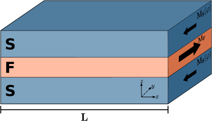
Figure 1: (Color online) Schematic representation of the considered SFS Josephson junction. The thickness of the F film is $2d_{\text{F}}$. The S films are assumed to be much thicker than the London penetration depth, i.e. $2d_{\text{S}}\gg\lambda_{\text{S}}$.

I Induced Magnetization in the Superconductor

In the following we derive a formula for the magnetization $M_{\text{S}}$ in the SFS junction induced in the S regions. The derivation is similar to that presented in Refs. Bergeret et al. (2004a); Volkov et al. (2019). Detailed calculations for the strong and weak proximity effect can be found in the Appendix A and B.

In the case of SFS Josephson junctions, one has to take into account the phase difference $\varphi$ which affects the energy spectrum and the density of states (DOS) in the F film. We assume a dirty limit which is described by the Usadel equations for the Green’s functions in the superconductor, $\check{g}_{\text{S}}$, and in the ferromagnet, $\check{g}_{\text{F}}$, respectively

$$-D_{\text{S}}\partial_{z}\quantity(\check{g}_{\text{S}}\partial_{z}\check{g}_{\text{S}})+\omega\quantity[\check{X}_{30},\check{g}_{\text{S}}]+\Delta\quantity[\check{X}_{10}\cos(\varphi/2)\pm\check{X}_{20}\sin(\varphi/2),\check{g}_{\text{S}}]=0,\quad\pm\text{S films}$$ (1)

$$-D_{\text{F}}\partial_{z}\quantity(\check{g}_{\text{F}}\partial\check{g}_{\text{F}})+\omega\quantity[\check{X}_{30},\check{g}_{\text{F}}]+iJ\quantity[\check{X}_{33},\check{g}_{\text{F}}]=0,\quad\text{F film}$$ (2)

where $\Delta$ is the superconducting gap and $\omega$ is the frequency. Here, $\check{X}_{ij}$ is defined as $\check{X}_{ij}=\hat{\tau}_{i}\otimes\hat{\sigma}_{j}$ with the Pauli matrices $\hat{\tau}$ and $\hat{\sigma}$ operating in particle-hole (Nambu-Gor’kov) and in spin space. The $\pm$S films denote the superconducting right (left) electrodes. Eqs.(1-2) are complemented by the normalization relation $\check{g}_{\text{S}(\text{F})}\cdot\check{g}_{\text{S}(\text{F})}=\check{1}$ and the boundary conditions Kurpianov and Lukichev (1988)

$$\check{g}_{\text{F}}\partial_{z}\check{g}_{\text{F}}=\kappa_{b\text{F}}\quantity[\check{g}_{\text{F}},\check{g}_{\text{S}}] ,\quad\quad\check{g}_{\text{S}}\partial_{z}\check{g}_{\text{S}}=\kappa_{b\text{S}}\quantity[\check{g}_{\text{S}},\check{g}_{\text{F}}]$$ (3)

where $\kappa_{b\text{S}(\text{F})}=\varrho_{\text{S}(\text{F})}/R_{b\square}$ with $\varrho_{\text{S}(\text{F})}$ being the resistivity of the S(F) film in the normal state and $R_{b\square}$ is a barrier resistance per unit square.

As in Refs. Bergeret et al., 2004a; Volkov et al., 2019, we assume that the Green’s functions $\check{g}_{\text{S}}$ in the S films are only weakly affected by the proximity effect. Thus, they can be written as

$$\check{g}_{\text{S}}^{(0)}=G_{\text{S}}\check{X}_{30}+F_{\text{S}}\quantity{\cos(\varphi/2)\check{X}_{10}\pm\sin(\varphi/2)\check{X}_{20}}$$ (4)

where $G_{\text{S}}=\omega/\zeta_{\omega}$ and $F_{\text{S}}=\Delta/\zeta_{\omega}$ are the normal and anomalous components of the Green’s function with $\zeta_{\omega}=\sqrt{\omega^{2}+\Delta^{2}}$. Assuming $d_{\text{F}}\ll\xi_{\text{F}}=\sqrt{D_{\text{F}}/J}$, Eq.(2) can be integrated over $z$ to obtain

$$\tilde{\omega}_{\text{F}}\quantity[\check{X}_{30},\check{g}_{\text{F}}]+\tilde{\Delta}_{\text{F}}\quantity[\check{X}_{10},\check{g}_{\text{F}}]+iJ\quantity[\check{X}_{33},\check{g}_{\text{F}}]=0,\quad\text{F film}$$ (5)

where $\tilde{\omega}_{\text{F}}=(\omega+\epsilon_{b\text{F}}G_{\text{S}})$, $\tilde{\Delta}_{\text{F}}(\varphi)=\epsilon_{b\text{F}}F_{\text{S}}\cos(\varphi/2)$ and $\epsilon_{b\text{F}}=D_{\text{F}}\kappa_{b\text{F}}/d_{\text{F}}$. At $z=\pm d_{\text{F}}$, the boundary conditions Eq.(3) are assumed to be identical, but with opposite signs. The Green’s functions are diagonal in spin space and the solution to Eq.(5) is

$$\hat{g}_{\text{F},\pm}=g^{(\text{F})}_{\pm}\hat{\tau}_{3}+f^{(\text{F})}_{\pm}\hat{\tau}_{1}$$ (6)

where the coefficients are given by $g^{(\text{F})}_{\pm}=\tilde{\omega}_{\pm}/\tilde{\zeta}_{\tilde{\omega}_{\pm}}(\varphi)$, $f^{(\text{F})_{\pm}}=\tilde{\Delta}_{\text{F}}(\varphi)/\tilde{\zeta}_{\tilde{\omega}_{\pm}}(\varphi)$ with $\tilde{\omega}_{\pm}=\tilde{\omega}_{\text{F}}\pm iJ$ and $\tilde{\zeta}_{\tilde{\omega}_{\pm}}(\varphi)=\sqrt{\tilde{\omega}_{\pm}^{2}+\tilde{\Delta}_{\text{F}}^{2}(\varphi)}$.

In order to find the induced magnetization in the superconductor S, we suppose that $\check{g}_{\text{S}}$ deviates weakly from its bulk value Eq.(4) and linearize Eq.(1). Then we can determine a small correction $\delta\check{g}_{\text{S}}$ to $\check{g}_{\text{S}}$

$$-\partial_{zz}\delta\check{g}_{\text{S}}+\kappa_{\text{S},\omega}^{2}\delta\check{g}_{\text{S}}=2\omega\delta\Delta\quantity(\omega\check{X}_{11}-\Delta\check{X}_{30})/D_{\text{S}}$$ (7)

where $\kappa_{\text{S},\omega}^{2}=2\sqrt{\omega^{2}+\Delta^{2}}/D_{\text{S}}$ and employed the relation $\delta\check{g}_{\text{S}}\cdot\check{g}_{\text{S}}^{(0)}+\check{g}_{\text{S}}^{(0)}\cdot\delta\check{g}_{\text{S}}=0$, which follows from the normalization condition. The induced magnetization is determined by the component $\delta g_{33}^{(\text{S})}=\Tr(\check{X}_{33}\delta\check{g}_{\text{S}})/4$ and is given by

$$M_{\text{S}}(z) =2\pi iT\mu_{B}\nu_{\text{S}}\sum_{\omega\geq 0}\delta g_{33}^{(\text{S})}(\pm d_{\text{F}})\exp(-\kappa_{\text{S},\omega}\absolutevalue{z\mp d_{\text{F}}})$$

$$\equiv-\sum_{\omega\geq 0}m_{\text{S}}(\varphi)\exp(-\kappa_{\text{S},\omega}\absolutevalue{z\mp d_{\text{F}}})$$ (8)

In the case of a strong PE i.e. ($R_{b\square}/\varrho_{\text{F}}<\sqrt{D_{\text{F}}/(d_{\text{F}}^{2}J)}$) (see also Appendix A), it is given by

$$m_{\text{S}}(\varphi)=M_{0}\frac{d_{\text{F}}}{\xi_{\text{S}}}\frac{2\pi T}{\Delta}\frac{(\tilde{\omega}^{2}+1)^{1/4}\cos[2](\varphi/2)}{(\tilde{\omega}^{2}+\cos[2](\varphi/2))^{3/2}}$$ (9)

where $D_{\text{F}}$ is the diffusion coefficient of the F film and $\xi_{\text{S}}^{2}=D_{\text{S}}/2\Delta$, $\tilde{\omega}=\omega/\Delta$ (see Appendix A). Here, the magnetic moment in the F film $M_{0}$ is given by $M_{0}=\mu_{B}\nu_{\text{F}}J$, where $\mu_{B}$ and $\nu_{\text{F}}$ are the effective Bohr magneton and the density of states in the F film, respectively.
In the case of a weak PE ($R_{b\square}/\varrho_{\text{F}}d_{\text{F}}>\sqrt{D_{\text{F}}/(d_{\text{F}}^{2}J)}$) the calculations are analogous (see Appendix B for details) and one finds

$$m_{\text{S}}(\varphi)= 4\mu_{B}\nu_{\text{S}}2\pi TG_{\text{S}}F_{\text{S}}^{2}\kappa_{b\text{S}}\kappa_{b\text{F}}\lambda_{\text{S}}$$

$$\times\Im{\frac{\cos[2](\varphi/2)+\sin[2](\varphi/2)\tanh[2](\theta_{\text{F}})}{\kappa_{\text{F},\omega}\tanh(\theta_{\text{F}})}}$$ (10)

where $\theta_{\text{F}}=\kappa_{\text{F},\omega}d_{\text{F}}$, $\kappa_{\text{F},\omega}^{2}=(\absolutevalue{\omega}+iJ_{\omega})/D_{\text{F}}$, $J_{\omega}=J\text{sign}(\omega)$ and $\lambda_{\text{S}}$ is the London penetration depth. Note that in the case of a strong PE the function $m_{\text{S}}(\varphi)$ does not contain the interface resistance $R_{b\square}$ while in the case of a weak PE it is proportional to $R_{b\square}^{-2}$.
In both cases, the induced magnetization in S depends on the phase difference $\varphi$. The total magnetic moment induced in the two superconductors $\mathcal{M}_{\text{S}}$ is determined by integration over $z$ . At zero temperature the summation over the Matsubara frequencies can be replaced by an integral ($2\pi T\sum_{\omega}(...)\Rightarrow\int_{0}^{\infty}\differential{\omega}(...)$). In particular we find the following expression for the case of a strong proximity effect

$$\mathcal{M}_{\text{S}}=-2d_{\text{F}}M_{0}\qquad\text{for}\quad\varphi\neq\pi$$ (11)

The magnetic moment induced in the superconductors does not depend on the phase difference $\varphi$ at any $\varphi$ except the points $\varphi_{n}=\pi(2n+1)$. It compensates exactly the total magnetic moment of the ferromagnetic film $\mathcal{M}_{\text{F}}=2d_{\text{F}}M_{0}$. The overall dependence $\mathcal{M}_{\text{S}}(\varphi)$ as a function of $\varphi$ is shown in Fig.2 for different temperatures $T$. At temperatures close to the critical temperature $T_{c}$ the dependence of $\mathcal{M}_{S}(\varphi)$ is almost sinusoidal. In the case of a weak PE, the total induced magnetization is much less than $2d_{\text{F}}M_{0}$.

Since the vectors $\mathbf{M}_{\text{S}}$ and $\mathbf{M}_{\text{F}}$ are aligned in the opposite directions, two identical magnetic granules embedded in a superconductor would interact antiferromagnetically with each other. Indeed, the magnetic moment $\mathbf{M}_{\text{S}}=-\mathbf{M}_{\text{F}1}$, produced by one granule with the magnetic moment $\mathbf{M}_{\text{F}1}$ will tend to orient the magnetic moment $\mathbf{M}_{\text{F}2}$ of another granule in the direction opposite to $\mathbf{M}_{\text{F}1}$. The characteristic length of this interaction is of the order of $\xi_{\text{S}}$ Bergeret et al. (2004a). There is a similarity between this case and the case considered in Ref. Yao et al. (2014), where it was found that at large distances the interaction between two magnetic impurities in a superconductor is antiferromagnetic one. However, the statement about antiparallel orientation of $\mathbf{M}_{\text{S}}$ and $\mathbf{M}_{\text{F}}$ is valid only for a diffusive superconductor. In the ballistic case the magnetization $M_{\text{S}}(z)$ oscillates in space Bergeret et al. (2005b); Kharitonov et al. (2006).

The dependence of the induced magnetization on the phase difference, leads to interesting phenomena. For example, if the current $I$ through the junction exceed the critical value $I_{c}$, the phase difference increases in time: $\varphi(t)=2eVt/\hbar$. This means that the induced magnetization $M_{\text{S}}(t)$ will oscillate in time with the Josephson frequency $\omega=2eV/\hbar$. Another interesting feature of spin polarization in SF systems is that in the case of a nonuniform magnetization $\mathbf{M}_{\text{F}}(\mathbf{r}_{\perp})$, the magnetization vector $\mathbf{M}_{\text{S}}(\mathbf{r}_{\perp})$ is an inverse mirror image of the vector $\mathbf{M}_{\text{F}}(\mathbf{r}_{\perp})$: $\mathbf{M}_{\text{S}}(\mathbf{r}_{\perp})=-\mathbf{M}_{\text{F}}(\mathbf{r}_{\perp})$. This relation is true if the characteristic length of the magnetization variation is much greater than the coherence length in S. For example, in the case of magnetic skyrmions, which can occur as topological structures in the magnetization profile of chiral ferromagnets, a skyrmion with opposite polarity arises in the S film. Since a Josephson junction is one of the most sensitive devices for probing the magnetic field, careful study of the influence of the magnetic field in SFS junctions can lead to the detection of the spin polarization in superconductors S.

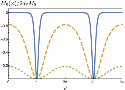
Figure 2: (Color online) The phase dependence of the total induced magnetization $\mathcal{M}_{\text{S}}(\varphi)$ for the strong proximity effect in the S film normalized by $2d_{\text{F}}M_{0}$ for various temperatures $\tilde{T}=T/T_{c}$ with $\tilde{T}=0.1$ (solid blue curve), $\tilde{T}=0.5$ (orange dashed curve) and $\tilde{T}=0.9$ (green dotted curve)

II Magnetostatics in SFS junction

In the following we proceed by considering the magnetostatics of a planar SFS Josephson junction with two identical SF interfaces. The $z$-axis is normal to the interface (see Fig.1) and the thickness of the F film is equal to $2d_{\text{F}}$. The magnetic properties of the considered system are described be the magnetic induction $\mathbf{B}=\curl{\mathbf{A}}$ and the magnetic field $\mathbf{H}$, which are related by the standard relation $\mathbf{B}=\mathbf{H}+4\pi\mathbf{M}$. The magnetization $\mathbf{M}$ exists not only in the F film ($\mathbf{M}_{\text{F}}$), but also in the superconducting region (as the induced magnetization $\mathbf{M}_{\text{S}}$). The magnetic field $\mathbf{H}$ obeys

$$\curl{\mathbf{H}}=\frac{4\pi}{c}\mathbf{j}$$ (12)

where $\mathbf{j}$ is the density of the Meissner current. It is connected to the vector potential $\mathbf{A}$ and the phase $\mathbf{\chi}$ of the order parameter via the standard gauge invariant expression

$$\mathbf{j}_{\text{S(\text{F})}}=-\frac{c}{4\pi}\quantity{\lambda_{\text{S}(\text{F})}^{-2}\quantity(\mathbf{A}-\frac{\Phi_{0}}{2\pi}\gradient{\chi})}$$ (13)

Here, $\lambda_{\text{S}(\text{F})}$ is the London penetration depths in S and F, respectively, and $\Phi_{0}=hc/2e$ is the magnetic flux quantum.

Our goal is to find the relation between an applied magnetic field $\mathbf{H}$ and the in-plane gradient $\gradient{\varphi}$ of the phase difference $\varphi$. We consider an in-plane magnetic field $\mathbf{H}=(0,H,0)$ and the in-plane magnetization $\mathbf{M}=(0,M(z),0)$ and we further set $\mathbf{A}=(A,0,0)$ and $\mathbf{j}=(j,0,0)$. Assuming that the $x$-dependence of all quantities of interest ($\mathbf{H}$ etc.) is weak on the length scale of the London penetration depth $\lambda_{\text{S}(\text{F})}$ we apply $\curl$ to the Maxwell equation, Eq.(12) and obtain the following equation for $\mathbf{H}_{\text{S}}$ in the S regions

$$\partial_{zz}^{2}H_{\text{S}}(x,z)-\lambda_{\text{S}}^{-2}H_{\text{S}}(x,z)=4\pi\lambda_{\text{S}}^{-2}M_{\text{S}}(z)$$ (14)

with the induced magnetization $M_{\text{S}}(z)$ given by Eqs.(8)-(9). Here, we employ the gauge $\divergence{\mathbf{H}}=0$ and use Eq.(13) for the current density $\mathbf{j}_{\text{S}}$. Eq.(14) is complemented by the boundary condition (see section Appendix C for details)

$$\quantity[\partial H_{\text{S}}(x)]=\lambda_{\text{S}}^{-2}\quantity(\quantity[A_{\text{S}}(x)]-\frac{\Phi_{0}}{2\pi}\partial_{x}\varphi(x))$$ (15)

where $\quantity[\partial H_{\text{S}}(x)]=\partial_{z}H_{\text{S}}(x,z)|_{z=d_{\text{F}}}-\partial_{z}H_{\text{S}}(x,z)|_{z=-d_{\text{F}}}$, $\quantity[A_{\text{S}}(x)]=A_{\text{S}}(x,d_{\text{F}})-A_{\text{S}}(x,-d_{\text{F}})$ and $\varphi(x)=\chi(x,d_{\text{F}})-\chi(x,-d_{\text{F}})$ is the phase difference across the junction. The difference $\quantity[A_{\text{S}}(x)]$ can be found by taking the continuity of the vector potential at the SF interfaces into account

$$\quantity[A_{\text{S}}(x)]=\quantity[A_{\text{F}}(x)]=2d_{\text{F}}\quantity(H_{0}(x)+4\pi M_{\text{F}})$$ (16)

Here, $H_{0}$ is an integration constant which approximately coincides with the magnetic field in F. The solution of Eq.(14) satisfying boundary condition has the form

$$H_{\text{S}}(x,z)= H_{orb}(x)\exp(-\lambda_{\text{S}}^{-1}\absolutevalue{z\mp d_{\text{F}}})$$

$$-4\pi\sum_{\omega\geq 0}\frac{m_{\text{S}}(\varphi)}{(\lambda_{\text{S}}\kappa_{\text{S},\omega})^{2}}\exp(-\kappa_{\text{S},\omega}\absolutevalue{z\mp d_{\text{F}}})$$ (17)

with

$$H_{orb}(x)=4\pi\sum_{\omega\geq 0}\frac{m_{\text{S}}(\varphi)}{(\lambda_{\text{S}}\kappa_{\text{S},\omega})}-\frac{d_{\text{F}}}{\lambda_{\text{S}}}\quantity(H_{0}(x)+4\pi M_{0})+\frac{\Phi_{0}}{4\pi\lambda_{\text{S}}}\partial_{x}\varphi$$ (18)

The short-ranged component, which decreases over the superconducting coherence length $\xi_{\text{S}}$, is a direct consequence of the inverse proximity effect. In addition, the spin polarization in the S results in a modification of the long-ranged component of the magnetic field (see Eq.(17)) which decays over the London penetration depth $\lambda_{\text{S}}$. Its amplitude $H_{orb}$ determines the magnetic field caused by orbital motion of the condensate (Meissner currents). The quantity $\kappa_{\text{S},\omega}$ is defined in Eq.(7). Note that the field $H_{0}(x)$ and the phase difference $\varphi$ are smoothly varying function of $x$. In the following, we assume that $\xi_{\text{S}}\ll\lambda_{\text{S}}$ i.e. neglecting the terms of the order of $\order{\xi_{\text{S}}/\lambda_{\text{S}}}$, so that $H_{\text{S}}(x,z)$ is dominated by the orbital contribution.
Next, we use the continuity condition for the field $H_{\text{S(\text{F})}}$ at at the interfaces $z=\pm d_{\text{F}}$ i.e. $H_{\text{S}}(x,\pm d_{\text{F}})=H_{\text{F}}(x,\pm d_{\text{F}})$ with $H_{\text{F}}(x,z)=H_{0}(x)+(H_{0}(x)+4\pi M_{0})\lambda_{\text{F}}^{-2}z^{2}/2$, and arrive to the following equation for $\varphi$

$$\partial_{\tilde{x}}\varphi(\tilde{x})=2\pi\quantity[\tilde{\Phi}_{m}(\tilde{x})-p_{\varphi}]$$ (19)

where $\tilde{x}=x/L$.
$\tilde{\Phi}_{m}(\tilde{x})$ and $p_{\varphi}$ are defined as

$$\tilde{\Phi}_{m}(\tilde{x})= \quantity{H_{0}(\tilde{x})L\quantity(2\lambda_{\text{S}}+2d_{\text{F}})+4\pi M_{0}L2d_{\text{F}}}/\Phi_{0}$$ (20)

$$p_{\varphi}= 2\gamma_{\varphi}\quantity{4\pi M_{0}L2d_{\text{F}}}/\Phi_{0}$$ (21)

In simple words, $\tilde{\Phi}_{m}$ and $p_{\varphi}$ are the normalized magnetic flux in the junction and a normalized $\varphi$-dependent contribution caused by spin polarization in S, respectively. The coefficient $\gamma_{\varphi}$ is given by

$$\gamma_{\varphi}=\frac{\xi_{\text{S}}}{2d_{\text{F}}M_{0}}\sum_{\omega\geq 0}\frac{m_{\text{S}}(\varphi)}{(\tilde{\omega}^{2}+1)^{1/4}}$$ (22)

with $\xi_{\text{S}}=\sqrt{D_{\text{S}}/2\Delta}$. The function $\gamma_{\varphi}$ is a periodic function of $\varphi$ and has different form in the limit of a strong and weak PE, see Appendices A and B for details. For temperatures, $T$, close to $T_{c}$, we get $\gamma_{\varphi}\cong\gamma_{0}\cos[2](\varphi/2)$, with $\gamma_{0}$ being a constant. If one considers $\gamma_{0,\varphi}=0$ i.e. no spin polarization, Eq.(19) coincides with the well known equation derived by Ferrel and Prange Ferrell and Prange (1963) (see also Kulik and Yanson (1972); Likharev (1979); Barone and Paterno (1982)). Then, the right-hand side of Eq.19 is the normalized magnetic flux in the junction $\tilde{\Phi}_{m}$ i.e. the flux related to the magnetic inductance $B(x)$. It consists of an external field $H_{ext}$, the magnetic field created by the Josephson current $I_{J}$ and the total magnetic moment of the F and the S. In the case of low barrier resistance and low temperatures $\gamma_{0}=1$, i.e. the flux coincides with the magnetic flux in the junction caused by an external magnetic field $H_{ext}$ as the magnetic flux in the F given by $4\pi M_{0}2d_{\text{F}}L$ is compensated by the magnetic flux in the S.

Another useful relation between $\tilde{\Phi}_{m}$ and $\varphi$ can be obtained from the Maxwell equation

$$\partialderivative{H_{0}(x)}{x}=\frac{4\pi}{c}j_{c}\sin(\varphi)$$ (23)

which after some straightforward algebra can be written as

$$\partialderivative{\tilde{\Phi}_{m}(\tilde{x})}{\tilde{x}}=r\sin(\varphi)$$ (24)

with $r=(4\pi L^{2}j_{c}/c)(2\lambda_{\text{S}}+2d_{\text{F}})/\Phi_{0}$. One can easily find the critical current $j_{c}$ in the case of a strong and a weak PE, which is given in the Appendix C in terms of microscopic parameters.
Finally, Eqs.(19)-(24) determine the relation between the ”magnetic” flux $\tilde{\Phi}_{m}$ and the phase difference $\varphi(x)$ in the presence of an induced magnetization $M_{\text{S}}(x)$. In principle, the non-linear Eqs.(19,24) can only be solved numerically. But we can still obtain analytic formulas assuming that the temperatures $T$ are close to $T_{c}$. The obtained results remain qualitatively unchanged for any $T\leq T_{c}$. Near $T_{c}$ Eq.(19) acquires the form

$$\partialderivative{\varphi(\tilde{x})}{\tilde{x}}=2\pi\quantity[\tilde{\Phi}_{m}(\tilde{x})-p\cos[2](\varphi/2)]$$ (25)

Here, the coefficient $p=2\gamma_{0}\quantity{4\pi M_{0}L2d_{\text{F}}}/\Phi_{0}$ is directly reflecting the strength of induced magnetic polarization effect in the S and can be easily expressed using Eq.(21) and Eq. (22) with the function $\gamma_{0}$ given in Eqs.(A7)-(B14) via $\gamma_{0}=\gamma_{\varphi}/\cos[2](\varphi/2)$(see Appendix C). The coefficient $r$, defined above, depends on the critical current $j_{c}$ and its form is given explicitly in the Appendix C as well. As we noted above, Eqs.(24),(25) can be solved numerically yet analytical expression in the limiting cases of $p<<r$ and $p>>r$ can also be obtained. Most importantly, to estimate how small $p$ is with respect to $r$, we rescale the quantities $p$, $p_{\varphi}$, $\tilde{\Phi}_{m}$ and $x$: $p_{r}=p/\sqrt{r}$, $\tilde{\Phi}_{m,r}(x)=\tilde{\Phi}_{m}/\sqrt{r}$ and $X=(x/L)\sqrt{r}$ yielding

$$\tilde{\Phi}_{m,r}(X)= \partial_{X}\varphi(X)+p_{r}\cos[2](\varphi(X)/2)$$ (26)

$$\partial_{X}\tilde{\Phi}_{m,r}(X)= \sin(\varphi(X))$$ (27)

One can see that if $p_{r}\ll 1$, that is, $p\ll\sqrt{r}$, the spin polarization in the S can be considered as a small correction. In the opposite limit, $p\gg\sqrt{r}$, the spin polarization of Cooper pairs leads to drastic changes, for example in the Fraunhofer pattern as we show below.

In the following we estimate parameters of the Josephson Nb/$\text{Cu}_{0.47}\text{Ni}_{0.53}$/Nb junctions studied experimentally Kontos et al. (2002). These parameters can be readily evaluated for this system as $2d_{\text{F}}=15\mbox{-}25\text{nm}$, $j_{c}=2\cdot 10^{4}\mbox{-}2\cdot 10^{3}\text{A}/\text{cm}^{2}$, the total interface resistance $R_{b}=30\mu\Omega$ for dimensions $L_{x}\times L_{y}=10\times 10\mu\text{m}^{2}$, $R_{b\square}=3\cdot 10^{-11}\Omega\cdot\text{cm}^{2}$, $D_{\text{F}}=5\text{cm}^{2}/s$, $\varrho_{\text{F}}=60\mu\Omega\cdot\text{cm}$, , $J=E_{ex}=850\text{K}$. Thus one finds $\varrho_{\text{F}}\cdot d_{\text{F}}=6\cdot 10^{-11}\Omega\cdot\text{cm}^{2}\geq R_{b\square}$ and the coherence length is $\xi_{\text{F}}=2.16\text{nm}$. For these parameters the factor $p$ appears to be small compared to $r$, so that the induced magnetization $M_{\text{S}}$ leads to rather small changes in the Josephson effect. For example, $p\sim 30\sqrt{I_{\theta}}\approx 0.3$ for $I_{\theta}\approx 10^{-4}$ and $p\sim 30\sqrt{I_{\theta}}\approx 3$ for $I_{\theta}\approx 10^{-2}$; here $I_{\theta}=\exp(-2\theta_{\text{F}})/\theta_{\text{F}}$. Nevertheless, it is instructive to investigate the Fraunhofer pattern for both small and large values of $p/r$ having in mind that in some other experimental realization of the SFS junction, the coeficient $p$ can be potentially larger.

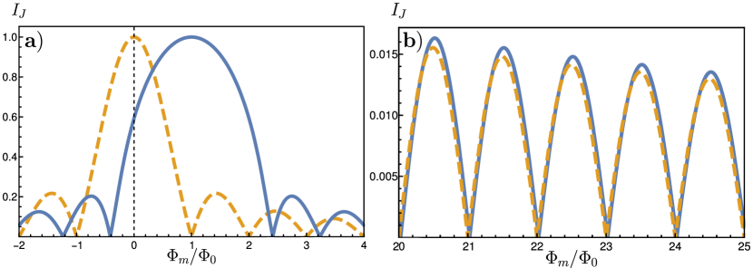
Figure 3: (Color online) a) The dependence of the critical current $\absolutevalue{\tilde{I}_{J}(\tilde{\Phi}_{m})}$ for $p=2$ (solid blue curve). The dashed (orange) line refers to the Fraunhofer pattern $\absolutevalue{\tilde{I}_{Fr}(\tilde{\Phi}_{m})}$ in the absence of of the spin polarization (SP) b) shows the same curves as in (a) but for larger values of $\Phi_{m}/\Phi_{0}$. One can see that the deviations from the standard Fraunhofer pattern becomes smaller with increasing $\Phi_{m}/\Phi_{0}$.

III Fraunhofer pattern

In this section, we begin with a brief discussion of the case where spin polarization in S leads to small corrections to the standard Fraunhofer pattern. Most of the remaining section is devoted towards the opposite case where the spin polarization plays a dominate role, resulting in a drastic change in the Fraunhofer pattern.

Weak spin polarization: $\mathbf{p\ll\sqrt{r}}$

Here, the phase difference $\varphi(\tilde{x})$ can be represented by: $\varphi(\tilde{x})=\varphi_{0}(\tilde{x})+\varphi_{1}(\tilde{x})+\varphi_{2}(\tilde{x})$, where $\varphi_{0}(\tilde{x})=\tilde{\Phi}_{m}\tilde{x}+c$ is an arbitrary constant determined by the requirement to maximize the current $I_{J}$. The normalized flux is given by $\tilde{\Phi}_{m}=\tilde{\Phi}_{m,0}+\tilde{\Phi}_{m,1}+\tilde{\Phi}_{m,2}$. In zero-order approximation the magnetic flux created by the current $I_{J}$ can be neglected and therefore $\tilde{\Phi}(\tilde{x})=\tilde{\Phi}_{ext}+\tilde{\Phi}_{\text{F}}+\tilde{\Phi}_{\text{S}}$. The constant $\tilde{\Phi}_{ext}$, $\tilde{\Phi}_{\text{F}}$ and $\tilde{\Phi}_{\text{S}}$ are defined as: $\tilde{\Phi}_{ext}=2\pi H_{ext}L(2d_{\text{F}}+2\lambda_{\text{S}})$, $\tilde{\Phi}_{\text{F}}=2\pi(4\pi M_{0}L2d_{\text{F}})/\Phi_{0}$ and $\tilde{\Phi}_{\text{S}}=2\pi(4\pi M_{0}L2d_{\text{F}}2\gamma_{0})/\Phi_{0}$. Expanding $\varphi(\tilde{x})$ and $\tilde{\Phi}(\tilde{x})$ we find the current

$$\tilde{I}_{\text{max}}=\frac{\sin(\pi\tilde{\Phi}_{m})}{\pi\tilde{\Phi}_{m}}+\delta\tilde{I}$$ (28)

Here the correction $\delta\tilde{I}$ contains small terms of the order $\tilde{p}^{2}/(2\Phi_{m,0}^{3})$ as well as $\sin(2\pi\tilde{\Phi}_{m})$, $\sin(3\pi\tilde{\Phi}_{m})$ etc., where $\tilde{p}\equiv(p+r/\tilde{\Phi}_{m,0})$ (see Appendix D for further details). At large $H_{ext}$ i.e. at large $\tilde{\Phi}_{m}$ the contribution from the spin polarization $p$ will dominated in $\tilde{p}$.

Strong spin polarization: $\mathbf{p\gg\sqrt{r}}$

In this case, our main approximation is a vanishing $r$, such that Eq.25 is described by a constant effective flux $\tilde{\Phi}_{m}(x)=\tilde{\Phi}_{m}$. Now, we can write the normalized current $\tilde{I}_{J}=I/Lj_{c}$ as

$$\tilde{I}_{J}=\frac{1}{L}\int_{0}^{L}\differential{x}\sin(\varphi(x))=\int_{\varphi_{0}}^{\varphi_{L}}\frac{\differential{\varphi}}{2\pi}\frac{\sin(\varphi)}{\tilde{\Phi}_{m}-p\cos[2](\varphi/2)}$$ (29)

with $\varphi_{L}=\varphi(L)$ and $\varphi_{0}=\varphi(0)$.

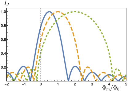
Figure 4: (Color online) Comparison of the dependence of the critical current $\absolutevalue{\tilde{I}_{J}(\tilde{\Phi}_{m})}$ for $p=1$ (blue solid line), $p=2$ (orange dashed line) and $p=4$ (green dotted line) .

After integration, we obtain

$$\tilde{I}_{J}= \frac{1}{\pi p}\ln(\frac{p-2\tilde{\Phi}_{m}+p\cos(\varphi_{L})}{p-2\tilde{\Phi}_{m}+p\cos(\varphi_{0})})$$

$$= \frac{1}{\pi p}\ln(\frac{a^{2}+T_{L}^{2}}{a^{2}+T_{0}}\frac{1+T_{0}^{2}}{1+T_{L}^{2}})$$ (30)

where $T_{L}=\tan(\varphi_{L}/2)$, $T_{0}=\tan(\varphi_{0}/2)$ and $a^{2}=(\tilde{\Phi}_{m}-p)/\tilde{\Phi}_{m}$. The quantities $T_{L}$ and $T_{0}$ are coupled via

$$L=\int_{0}^{L}\differential{x}=L\int_{\varphi_{0}}^{\varphi_{L}}\frac{\differential{\varphi}}{2\pi}\frac{1}{\tilde{\Phi}_{m}-p\cos[2](\varphi/2)}$$ (31)

Calculating the integral, we obtain the relation

$$T_{L}=\frac{T_{0}+ba^{2}}{1+bT_{0}}$$ (32)

with $b=a^{-1}\tan(\pi a\tilde{\Phi}_{m})$. So far, Eq.(30,32), determine the critical current $\tilde{I}_{J}$ as a function of an arbitrary constant $T_{0}\equiv\tan(\varphi_{0}/2)$. In order to find the maximum of the current $\tilde{I}_{J}$, we need to determine the value of $T_{0}$ which maximizes the current. The roots of the equation $\partial\tilde{I}_{J}/\partial T_{0}=0$ are given by

$$T_{m}= \frac{1}{2a}\left(-(1+a^{2})\tan(\pi a\tilde{\Phi}_{m})\right.$$

$$\left.\pm\sqrt{4a^{2}+(1+a^{2})^{2}\tan[2](\pi a\tilde{\Phi}_{m})}\right)$$ (33)

Substituting $T_{m}$ into Eq.(30) and using Eq.(32), we can extract the solution for the maximal current $\tilde{I}_{J}(\tilde{\Phi}_{m})$. The result is shown in Fig.3 for $p=2$ characterizing a finite contribution from the spin polarization. The dependence $\tilde{I}_{J}(\tilde{\Phi}_{m})$ is compared with the standard Fraunhofer pattern in the absence of the spin polarization

$$I_{Fr}(\Phi_{m}/\Phi_{0})=\absolutevalue{\frac{\sin(\pi\Phi_{m}/\Phi_{0})}{\pi\Phi_{m}/\Phi_{0}}}$$ (34)

where $\Phi_{m}=L\quantity{H_{0}\quantity(2\lambda_{\text{S}}+2d_{\text{F}})+4\pi M_{0}2\lambda_{\text{S}}}$.

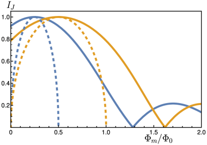
Figure 5: (Color online) Comparison of the solution of the critical current $\absolutevalue{\tilde{I}_{J}(\tilde{\Phi}_{m})}$ in Eq.(30) (solid lines) and $\tilde{I}_{J,ad}=\sqrt{1-(2\tilde{\Phi}_{m}-p)^{2}/p^{2}}$ (dashed lines) for $p=0.5$ (blue line) and $p=1$ (orange line).

One can see that for small values of $p$, the behavior of the critical current $\absolutevalue{I_{J}(\tilde{\Phi}_{m})}$ resembles the shape of the classical Fraunhofer pattern, whereas for increasing $p$, the difference become more pronounced (see also Fig.4). In particular, the induced spin polarization causes a shift of the global maximum of the critical current by an amount of $p/2$. This shift occurs in addition to the displacement of the global maximum caused by the magnetization in the ferromagnet(see Refs. Banerjee et al. (2014); Glick et al. (2017); Satchell and Birge (2018)), so that its position is effectively changed by the amount $4\pi M_{0}L2d_{\text{F}}\quantity[1-\gamma_{0}]$. Notice that for $\gamma_{0}=1$, both displacements cancel each other, so there is no shift.
Most importantly, the spin polarization causes a broadening of the peaks of the Fraunhofer pattern. This effect is most pronounced for the main maximum (see Fig.3). In contrast to the shift, the broadening is only determined by the strength of the induced spin polarization and is as such a direct consequence of the inverse proximity effect. The broadening is stronger for larger $p$ (see Fig.5)
If one compares the changes of the Fraunhofer pattern for large values $\Phi_{m}/\Phi_{0}$ (see Fig.3b), one recognizes that the differences to the standard pattern disappear.

It should be noted that for $\tilde{\Phi}_{m}\leq p$, one can obtain another solution for Eq.(25) with a space-independent phase difference $\varphi_{ad}$

$$\cos(\varphi_{ad})=(2\tilde{\Phi}_{m}-p)/p$$ (35)

However, the current $\tilde{I}_{J,ad}=\sqrt{1-(2\tilde{\Phi}_{m}-p)^{2}/p^{2}}$ corresponding to this solution is less than the current $\tilde{I}_{J}$ given by Eq.(30) (see Fig.5). Thus, the Josephson energy $E_{J,ad}\sim I_{J,ad}(1-\cos(\varphi_{ad}))$ is somewhat higher than the Josephson energy related to the current $\tilde{I}_{J}$. Since the difference between these currents is small, transitions between two different solution for the current $\tilde{I}_{J}$ are possible at small $\tilde{\Phi}_{m}$. Note that some instabilities in the dependence of $I_{J}(H_{ext})$ are observed in the experiment Banerjee et al. (2014); Glick et al. (2017); Satchell and Birge (2018).
One can easily show that for $p\rightarrow 0$, the dependence $\absolutevalue{\tilde{I}_{J}(\tilde{\Phi}_{m})}$ is reduced to $\absolutevalue{\tilde{I}_{Fr}(\tilde{\Phi}_{m})}$. In this limit we have $a\cong 1-2p/\tilde{\Phi}$ and Eq.(30) takes the form

$$\tilde{I}_{J}(\tilde{\Phi}_{m})\approx\frac{1}{\pi\tilde{\Phi}_{m}}\quantity[\frac{1}{1+T_{0}^{2}}-\frac{1}{1+T_{L}^{2}}]$$ (36)

Substituting Eq.(32,33) with $a=1$, we obtain Eq.(34).

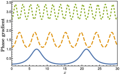
Figure 6: (Color online) Coordinate dependence of the phase gradient $\partial\varphi(\tilde{x})/\partial\tilde{x}$ for different $\tilde{\Phi}_{m}$ but fixed $p=0.4$: $\tilde{\Phi}_{m}=0.6$ (blue line), $\tilde{\Phi}_{m}=1.5$ (orange line) and $\tilde{\Phi}_{m}=3$ (green line).

We also provide an expression for the coordinate dependence for the phase difference $\varphi$ which can be obtained from Eq.(25)

$$\partialderivative{\varphi}{\tilde{x}}=\frac{\tilde{\Phi}_{m}^{2}-p^{2}}{\tilde{\Phi}_{m}+p\cos(\kappa(\tilde{x}-\tilde{x}_{0}))}$$ (37)

where $\kappa=\sqrt{\tilde{\Phi}_{m}^{2}-p^{2}}$. This dependence describes a fluxon in a long SFS Josephson junction i.e. $L\gg\lambda_{J}$ with the Josephson length $\lambda_{J}$ (see Fig.6). One can see that at $\tilde{\Phi}_{m}$ close to $p$, the fluxons have the form of narrow spikes. At $\tilde{\Phi}_{m}\gg p$, this dependence has the form of a sinusoidal function. Note that the dependence $\partial\varphi(\tilde{x})/\partial\tilde{x}$ given by this equation coincides with the temporal dependence of the voltage $V(t)$ at different currents $I$ in a point superconducting contact if the following replacements are made: $V\rightarrow\partial\varphi(\tilde{x})/\partial\tilde{x}$; $I/I_{c}\rightarrow\tilde{\Phi}_{m}$; $t\rightarrow\tilde{x}$; $p=1$ ($I_{c}$ is the critical current)Aslamazov and Larkin (1969).

IV Conclusion

In this manuscript, we studied the influence of the spin polarization of Cooper pairs in superconductors on the Josephson effect in SFS junctions. The expression for the induced magnetization $M_{\text{S}}$ was obtained in the cases of low and large SF interface resistances $R_{b\square}$. We have shown that the magnetization $M_{\text{S}}$ depends on the phase difference $\varphi$ so that for $I>I_{c}$ it oscillates in time with the Josephson frequency $\omega=2eV/\hbar$. The induced spin polarization in the S, contributes to the orbital motion of the condensate (Meissner currents), resulting in a long-ranged magnetic field contribution penetrating the superconductor over the length scale of the London penetration depth $\lambda_{\text{S}}$. Since the magnetic flux in the junction is not only determined by an applied external magnetic field $\mathbf{H}_{ext}$ but also by the total magnetic moment $\mathbf{M}_{tot}=\mathbf{M}_{\text{F}}+\mathbf{M}_{\text{S}}$, the Fraunhofer pattern depends on the induced magnetization $\mathbf{M}_{\text{S}}$. In particular, at low $R_{b\square}$ and low temperatures $T$, the total magnetization may turn to zero: $\mathbf{M}_{\text{F}}+\mathbf{M}_{\text{S}}=0$ (full magnetic screening). With a suitable choice of parameters the Fraunhofer pattern modifies drastically. For example, the spin polarization in the S causes a shift of the Fraunhofer pattern, which is opposite to the displacement by the magnetization in the F. However, even more significant is a broadening of the Fraunhofer peaks, which is particularly pronounced for the peak corresponding to the global maximum. These changes are most notable for a small magnetic flux, such that one should look for features of the spin polarization in the first series of peaks. Thus we conclude that a careful analysis of the Josephson effect in SFS structures (for example, of the dependence of $I_{J}(H_{ext})$) may reveal the presence of the spin polarization in superconductors.

V Acknowledgement

The authors acknowledge support from the Deutsche Forschungsgemeinschaft Priority Program SPP2137, Skyrmionics, under Grant No. ER 463/10.

Appendix A Strong Proximity Effect

In the following we present several limiting cases for the magnetization in the superconductor for a strong proximity effect. We start by multiplying Eq.(7) by $\check{X}_{33}$ and calculate the trace. Then, the right-hand side of Eq.(7) is zero and we find a solution

$$\delta g_{33}^{(\text{S})}(z)=\delta g_{33}^{(\text{S})}(\pm d_{\text{F}})\exp(-\kappa_{\text{S},\omega}\absolutevalue{z\mp d_{\text{F}}})$$ (A1)

The integration constant is found from the boundary condition Eq.(3) that yields

$$\partial_{z}\delta g_{33}^{(\text{S})}(z)|_{z=\pm d_{\text{F}}}=\mp 2\kappa_{b\text{S}}F_{\text{S}}\quantity(F_{\text{S}}g_{33}^{(\text{F})}-G_{\text{S}}g_{13}^{(\text{F})}\cos(\varphi/2))$$ (A2)

where $g_{13}^{(\text{F})}=\epsilon_{b\text{F}}i\Im{1/\tilde{\zeta}_{\tilde{\omega}_{+}}(\varphi)}$ and $g_{33}^{(\text{F})}=i\Im{\tilde{\omega}_{+}/\tilde{\zeta}_{\tilde{\omega}_{+}}(\varphi)}$. The function $\tilde{\zeta}_{\tilde{\omega}_{\pm}}(\varphi)$ is: $\tilde{\zeta}_{\tilde{\omega}_{\pm}}(\varphi)=\sqrt{\tilde{\omega}_{\pm}^{2}+\tilde{\Delta}_{\text{F}}^{2}(\varphi)}$.
We obtain for $\delta g_{33}^{(S)}(z)$

$$\delta g_{33}^{(S)}(z)=\frac{2\kappa_{b\text{S}}}{\kappa_{\text{S},\omega}}F_{\text{S}}\quantity(F_{\text{S}}g_{33}^{(F)}-G_{\text{S}}g_{13}^{(F)}\cos(\varphi/2))\exp(-\kappa_{\text{S},\omega}\absolutevalue{z\mp d_{\text{F}}})=\delta g_{33}^{(S)}(\pm d_{\text{F}})\exp(-\kappa_{\text{S},\omega}\absolutevalue{z\mp d_{\text{F}}})$$ (A3)

One can see that this correction $\delta\check{g}_{\text{S}}$ is small if the condition $\kappa_{b\text{S}}\xi_{\text{S}}\ll 1$ is fulfilled, that is, $R_{b\square}\gg\varrho_{\text{S}}\xi_{\text{S}}$.
Consider the case where $\Delta\ll J\ll\epsilon_{b\text{F}}$. In this limit $\tilde{\omega}_{+}\approx\epsilon_{b\text{F}}(G_{\text{S}}+iJ)$ and $\tilde{\zeta}_{\tilde{\omega}_{+}}(\varphi)=\epsilon_{b\text{F}}\zeta_{\varphi}(1+i\tilde{J}G_{\text{S}}/\zeta_{\varphi}^{2})$. The function $g_{13}^{(\text{F})}$ and $g_{33}^{(\text{F})}$ are equal to

$$g_{13}^{(\text{F})}= -\frac{i\tilde{J}}{\zeta_{\varphi}}\frac{G_{\text{S}}F_{\text{S}}\cos(\varphi/2)}{\zeta_{\varphi}^{2}}$$ (A4)

$$g_{13}^{(\text{F})}= \frac{i\tilde{J}}{\zeta_{\varphi}}\frac{F_{\text{S}}^{2}\cos[2](\varphi/2)}{\zeta_{\varphi}^{2}}$$ (A5)

with $\tilde{J}=J/\epsilon_{b\text{F}}$, $\zeta_{\varphi}=\sqrt{G_{\text{S}}^{2}+F_{\text{S}}\cos[2](\varphi/2)}$. By using Eq.(A3), we obtain for $\delta g_{33}^{(\text{S})}(\pm d_{\text{F}})$

$$\delta g_{33}^{(\text{S})}(\pm d_{\text{F}})=\frac{i\tilde{J}\kappa_{b\text{S}}}{\kappa_{\text{S},\omega}}\frac{2F_{\text{S}}^{2}\cos[2](\varphi/2)}{\zeta_{\varphi}}$$ (A6)

The magnetization $M_{\text{S}}(z)$ in Eq.(8) is expressed through the function $m_{\text{S}}(\varphi)$ that is given in Eq.(9). Near $T_{c}$ we obtain for $\gamma_{\varphi}$ (see Eq.(22))

$$\gamma_{\varphi}=\quantity(\frac{\Delta}{\pi T})^{2}2\cos[2](\varphi/2)\sum_{n\geq 0}(2n+1)^{-3}$$ (A7)

Appendix B Weak Proximity Effect

Consider an SFS junction with a high interface resistance so that only a weak PE occurs. Then the condensate wave function $\check{f}$ is small and we can linearized Eq.(1). In the F film, the function $\check{f}_{\text{F}}$ obeys the equation

$$\partial_{zz}^{2}\hat{f}_{\text{F}\pm}-\kappa_{\text{F}\pm}^{2}\hat{f}_{\text{F}\pm}=0,\quad\text{F film}$$ (B1)

where $\kappa_{\text{F}\pm}^{2}=2(\absolutevalue{\omega}\pm iJ_{\omega})/D_{\text{F}}$ with $J_{\omega}=J\text{sign}(\omega)$. In zeroth order approximation, the Green’s functions in the S films have the form

$$\hat{g}_{\text{S}}^{(0)}(\pm d_{\text{F}})=G_{\text{S}}\hat{\tau}_{3}+F_{\text{S}}\quantity{\cos(\varphi/2)\hat{\tau}_{1}\pm\sin(\varphi/2)\hat{\tau}_{2}}$$ (B2)

The solution of Eq.(B1) is

$$\hat{f}_{\text{F}\pm}(z)=\hat{C}_{\pm}\cosh(\kappa_{\text{F}\pm}z)+\hat{S}_{\pm}\sinh(\kappa_{\text{F}\pm}z)$$ (B3)

Integration constants are found from the BCs Kurpianov and Lukichev (1988)

$$\partial_{z}\hat{f}_{\text{F},\pm}(\pm d_{\text{F}})=\pm 2\kappa_{b\text{F}}F_{\text{S}}\quantity{\cos(\varphi/2)\hat{\tau}_{1}\pm\sin(\varphi/2)\hat{\tau}_{2}}$$ (B4)

We find

$$\hat{C}_{\pm}= \frac{2\kappa_{b\text{F}}}{\kappa_{\text{F}\pm}}\frac{F_{\text{S}}\cos(\varphi/2)}{\sinh(\kappa_{\text{F}\pm}d_{\text{F}})}\hat{\tau}_{1}$$ (B5)

$$\hat{S}_{\pm}= \frac{2\kappa_{b\text{F}}}{\kappa_{\text{F}\pm}}\frac{F_{\text{S}}\sin(\varphi/2)}{\cosh(\kappa_{\text{F}\pm}d_{\text{F}})}\hat{\tau}_{2}$$ (B6)

One can write for $\check{f}(\pm d_{\text{F}})$

$$\check{f}(\pm d_{\text{F}})=2\kappa_{b\text{F}}F_{\text{S}}\quantity(\cos(\varphi/2)\quantity{\quantity(\check{X}_{10}\real\pm i\check{X}_{13}\imaginary)\frac{1}{\kappa_{\text{F},\omega}\tanh(\kappa_{\text{F},\omega}d_{\text{F}})}}+\sin(\varphi/2)\quantity{\quantity(\check{X}_{20}\real\pm i\check{X}_{23}\imaginary)\frac{\tanh(\kappa_{\text{F},\omega}d_{\text{F}})}{\kappa_{\text{F},\omega}}})$$ (B8)

where $\kappa_{\text{F},\omega}^{2}=2(\absolutevalue{\omega}+iJ_{\omega})/D_{\text{F}}$.
The linearized Eq.(7) can be written as follows

$$-\partial_{zz}^{2}\delta g_{33}^{(\text{S})}+\kappa_{\text{S},\omega}^{2}\delta g_{33}^{(\text{S})}=0$$ (B9)

The BC to Eq.(B9) is

$$\partial_{z}\delta g_{33}^{(S)}(\pm d_{\text{F}})=-\kappa_{b\text{S}}\quantity(\check{g}_{\text{F}}-\check{G}_{\text{S}}\check{g}_{\text{F}}\check{G}_{\text{S}})_{33}$$ (B10)

or

$$\partial_{z}\delta g_{33}^{(S)}(\pm d_{\text{F}})=4\kappa_{b\text{S}}\kappa_{b\text{F}}G_{\text{S}}F_{\text{S}}^{2}i\Im{\frac{\cos[2](\varphi/2)+\sin[2](\varphi/2)\tanh[2](\kappa_{\text{F},\omega}d_{\text{F}})}{\kappa_{\text{F},\omega}\tanh[2](\kappa_{\text{F},\omega}d_{\text{F}})}}$$ (B11)

Here, we have taken into account that the correction $g_{33}^{(\text{F})}\sim f_{13}^{2}$ is small. The solution for Eq.(B9) is

$$\delta g_{33}^{(\text{S})}(z)=\delta g_{33}^{(\text{S})}(\pm d_{\text{F}})\exp(-\kappa_{\text{F},\omega}\absolutevalue{z-d_{\text{F}}})$$ (B12)

with

$$\delta g_{33}^{(S)}(\pm d_{\text{F}})=4G_{\text{S}}F_{\text{S}}^{2}i\frac{\kappa_{b\text{S}}\kappa_{b\text{F}}}{\kappa_{\text{S},\omega}}\Im{\frac{\cos[2](\varphi/2)+\sin[2](\varphi/2)\tanh[2](\theta_{\text{F}})}{\kappa_{\text{F},\omega}\tanh[2](\theta_{\text{F}})}}$$ (B13)

where we defined $\theta_{\text{F}}=\kappa_{\text{F},\omega}d_{\text{F}}$.
Using this expression we obtain Eq.(10) for the spin polarization in superconductors S. Close to $T_{c}$ the coefficient $\gamma_{\varphi}$ is equal to

$$\gamma_{\varphi}=4\sqrt{2}\frac{\xi_{\text{S}}}{d_{\text{F}}}\frac{\kappa_{b\text{S}}\kappa_{b\text{F}}}{\kappa_{\text{S},\omega}\kappa_{\text{F}c}}\frac{2T}{J}\Im{\frac{\cos[2](\varphi/2)+\sin[2](\varphi/2)\tanh[2](\theta_{\text{F}c})}{(1+i)\tanh(\theta_{\text{F}c})}}\frac{\Delta^{2}}{\pi T}\sum_{\omega\geq 0}(2n+1)^{-3}$$ (B14)

where $\theta_{\text{F}c}=\kappa_{\text{F}c}d_{\text{F}}(1+i)/\sqrt{2}$, $\kappa_{\text{F}c}=\sqrt{J/D_{\text{F}}}$, and $\sum_{n}(2n+1)^{-3}=8\zeta(3)/8$ with the Riemann zeta function $\zeta(x)$.

Appendix C Magnetostatics

The boundary conditions for Eq.(16) can be easily obtained from

$$\partial_{z}H_{\text{S}}(x,z)|_{z=\pm d_{\text{F}}}=\lambda_{\text{S}}^{-2}\quantity[A_{\text{S}}(x,z)-\frac{\Phi_{0}}{2\pi}\partial_{x}\chi(x,z)]_{z=\pm d_{\text{S}}}$$ (C1)

Subtracting the expression for Eq.(13) at the interfaces $z=d_{\text{F}}$ and $z=-d_{\text{F}}$, we obtain Eq.(15) with $\quantity[A_{\text{S}}(x)]=A_{\text{S}}(x,d_{\text{F}})-A_{\text{S}}(x,-d_{\text{F}})$ and $\varphi(x)=\chi(x,d_{\text{F}})-\chi(x,-d_{\text{F}})$. The difference $[A_{S}(x)]$ can be found by taking into account the variation of the vector potential in the F film. The latter can be easily found in the limit $\lambda_{\text{F}}\gg d_{\text{F}}$ (see Ref.Volkov et al. (2019))

$$A_{\text{F}}(x,z)\cong \quantity(H_{0}(x)+4\pi M_{0})\quantity(1+\frac{\kappa_{\text{F}}^{2}z^{2}}{2})z$$ (C2)

$$B_{\text{F}}(x,z)\cong \quantity(H_{0}(x)+4\pi M_{0})\quantity(1+\frac{\kappa_{\text{F}}^{2}z^{2}}{2})$$ (C3)

$$H_{\text{F}}(x,z)\cong H_{0}(x)\quantity(1+\frac{\kappa_{\text{F}}^{2}z^{2}}{2})+4\pi M_{0}\frac{\kappa_{\text{F}}^{2}z^{2}}{2}$$ (C4)

where we set $M_{\text{F}}\approx M_{0}$ since corrections to $M_{0}$ in the F film due to the proximity effect are small and do not significantly change the final results. For completness, we also write down the formulas for the fields $B_{\text{F}}(x,z)$ and $H_{\text{F}}(x,z)$.

Appendix D Critical Current

The josephson current density across the junction can be be obtained using

$$j_{J}(\varphi)= i\sigma_{\text{F}}\frac{2\pi T}{e}\sum_{\omega\geq 0}\frac{1}{4}\Tr{\check{X}_{30}\check{g}_{\text{F}}(z)\partial_{z}\check{g}_{\text{F}}(z)}$$ (D1)

$$= i\sigma_{\text{F}}\frac{2\pi T}{e}\kappa_{b\text{F}}\sum_{\omega\geq 0}\frac{1}{4}\Tr{\check{X}_{30}\quantity[\check{g}_{\text{F}}(d_{\text{F}}),\check{g}_{\text{S}}]}$$ (D2)

where $\sigma_{\text{F}}$ is the conductivity of the F.
In the second line, we used the boundary condition Eq.(3). At temperatures close to $T_{c}$, the Josephson current $j_{J}(\varphi)$ can be written as follows

$$j_{J}(\varphi)=j_{c}\sin(\varphi)$$ (D3)

One can find the critical current density $j_{c}$ in the limit of a strong and a weak PE by using Eqs.(6,B3,)

$$j_{c}=\frac{\pi T}{eR_{b\square}}\sum_{\omega\geq 0}F_{\text{S}}^{2}\cong\frac{\pi\Delta^{2}}{8eR_{b\square}T}$$ (D4)

where in the the case of a strong PE we get

$$j_{c}= \sigma_{\text{F}}\frac{2\pi T}{e}4\kappa_{b\text{F}}^{2}\Re{\sum_{\omega\geq 0}\frac{F_{\text{S}}}{\kappa_{\text{F},\omega}\sinh(2\theta_{\text{F}})}}$$ (D5)

$$\cong \frac{\pi\sigma_{\text{F}}}{\sqrt{2}}\frac{\Delta^{2}}{eT}\kappa_{b\text{F}}^{2}d_{\text{F}}\xi_{\text{F}}\frac{\sinh(\alpha)\cos(\alpha)-\cosh(\alpha)\sin(\alpha)}{\kappa_{\text{F}}\sinh(2\theta_{\text{F}})}$$ (D6)

and in the case of a weak PE. Here $\alpha=\sqrt{2}d_{\text{F}}/\xi_{\text{F}}$, $\xi_{\text{F}}=\sqrt{D_{\text{F}}/J}$. For large $\alpha$ we can rewrite Eq.(D5) as

$$j_{c}= \sigma_{\text{F}}\frac{2\pi T}{e}4\kappa_{b\text{F}}^{2}\Re{\sum_{\omega\geq 0}\frac{F_{\text{S}}}{\kappa_{\text{F},\omega}\sinh(2\theta_{\text{F}})}}$$ (D7)

$$\cong -\pi\sigma_{\text{F}}\frac{\Delta^{2}}{eT}\kappa_{b\text{F}}^{2}d_{\text{F}}\xi_{\text{F}}\exp(-\alpha)\sin(\alpha-\pi/4)$$ (D8)

D.1 Small Contribution of the Spin Polarization

We expand the phase difference $\varphi(\tilde{x})$ up to the second order and write the integral in Eq.(29) in the form

$$I_{J}= j_{c}\int_{0}^{1}\sin(\varphi(\tilde{x}))\differential{\tilde{x}}$$ (D9)

$$\cong j_{c}\int_{1/2}^{-1/2}\quantity[\sin(\varphi_{0})+\varphi_{1}\cos(\varphi_{0})-\varphi_{2}\sin(\varphi_{0})+\frac{\varphi_{1}}{2}\cos(\varphi_{0})]\differential{\tilde{x}}$$ (D10)

We need to find $\varphi_{i}$ and $\tilde{\Phi}_{m}$. In the zeroth order approximation we obtain

$$\varphi_{0}=\tilde{\Phi}_{m,0}\tilde{x}+c$$ (D11)

where $\tilde{\Phi}_{m,0}=2\pi(H_{ext}(2d_{\text{F}}+2\lambda_{\text{S}})+4\pi M_{0}2d_{\text{F}})/\Phi_{0}$. In the first approximation, we get from Eqs.(24,25)

$$\tilde{\Phi}_{m,1}=-\frac{r}{\tilde{\Phi}_{m,0}}\cos(\varphi_{0})\qquad\varphi_{1}=-\frac{\tilde{p}}{\tilde{\Phi}_{m,0}}\sin(\varphi_{0})$$ (D12)

where $\tilde{p}=p+r/\tilde{\Phi}_{m,0}$. For the second order contribution we obtain

$$\tilde{\Phi}_{m,2}= \frac{r\tilde{p}}{(2\tilde{\Phi}_{m,0})^{2}}\cos(2\varphi_{0})$$ (D13)

$$\varphi_{2}= -\frac{p\tilde{p}}{2\tilde{\Phi}_{m,0}}\tilde{x}+\frac{\tilde{p}}{(2\tilde{\Phi}_{m,0})^{2}}\quantity(p+\frac{r}{2\tilde{\Phi}_{m,0}})\sin(2\varphi_{0})$$ (D14)

The current $\tilde{I}_{J}\equiv I_{J}/j$ can be written as

$$\tilde{I}_{J}=\tilde{I}_{Fr}+\delta\tilde{I}_{0}+\delta\tilde{I}_{2}+\delta\tilde{I}_{3}$$ (D15)

where

$$\tilde{I}_{Fr}= \int_{1/2}^{-1/2}\sin(\varphi_{0})\differential{\tilde{x}}$$ (D16)

$$\delta I_{0}= \delta a\sin(c)$$ (D17)

$$\delta I_{2}= \int_{1/2}^{-1/2}\quantity[\varphi_{2}\cos(\varphi_{0})-\frac{\varphi_{1}^{2}}{2}\sin(\varphi_{0})]\differential{\tilde{x}}\$$ (D18)

By using Eqs.(D10-D18), we find

$$\tilde{I}_{0}= a_{Fr}\sin(c)$$ (D19)

$$\delta\tilde{I}_{0}= \delta a\sin(c)$$ (D20)

$$\delta\tilde{I}_{2}= -\lambda_{2}\sin(2c)$$ (D21)

$$\delta\tilde{I}_{3}= \delta a\tilde{I}_{0}+\lambda_{3}\sin(3c)$$ (D22)

where $a=a_{Fr}+\delta a$, $a_{Fr}=(2/\tilde{\Phi}_{m,0})\sin(\tilde{\Phi}_{m,0}/2)$, $\delta a=\quantity{-\tilde{p}^{2}/2\tilde{\Phi}_{m,0}^{3}+\tilde{p}r/(2\tilde{\Phi}_{m,0})^{4}}\sin(\tilde{\Phi}_{m,0}/2)$, $\lambda_{2}=-2\tilde{p}/(2\tilde{\Phi}_{m,0})^{2}\sin(\tilde{\Phi}_{m,0})$ and $\lambda_{3}=\quantity{(2p+3r/2\tilde{\Phi}_{m,0})\tilde{p}/(12\tilde{\Phi}_{m,0}^{3})}\sin(3\tilde{\Phi}_{m,0}/2)$. The quantities $\lambda$ are assumed to be small: $\lambda<<1$. We have to find the maximum of $\tilde{I}_{J}$ as a function of the constant $c$ by expanding the current in powers of $\lambda$: $c=c_{0}+c_{1}+c_{2}$. Calculating the derivative $\partial\tilde{I}_{J}/\partial c$, we find

$$c_{0}=\frac{\pi}{2},\quad c_{1}=-2\frac{\lambda_{1}}{a},\qquad c_{2}=0$$ (D23)

Thus the maximal current is equal to

$$\tilde{I}_{J}=\frac{2}{\tilde{\Phi}_{m,0}}\sin(\tilde{\Phi}_{m,0}/2)+\delta\tilde{I}_{J}$$ (D24)

The first term is the standard Fraunhofer pattern and the second term is a correction due to spin polarization ($\sim p$) and due to the finite length $L$ compared to the Josephson length $\lambda_{J}$. This correction is

$$\delta\tilde{I}_{J}=\sin(\tilde{\Phi}_{m,0}/2)\quantity[-\frac{2\tilde{p}}{(\tilde{\Phi}_{m,0})^{3}}+\frac{pr}{(2\tilde{\Phi}_{m,0})^{4}}]+\frac{\tilde{p}}{2\tilde{\Phi}_{m,0}^{3}}\sin(\tilde{\Phi}_{m,0})\cos(\tilde{\Phi}_{m,0}/2)-\frac{\tilde{p}(\tilde{p}+(p+r/2\tilde{\Phi}_{m,0}))}{24\tilde{\Phi}_{m,0}^{3}}\sin(3\tilde{\Phi}_{m,0}/2)$$ (D25)

References

- Golubov et al. (2004) A. A. Golubov, M. Y. Kupriyanov, and E. Il’ichev, Rev. Mod. Phys. 76, 411 (2004).
- Buzdin (2005) A. I. Buzdin, Rev. Mod. Phys. 77, 935 (2005).
- Bergeret et al. (2005a) F. S. Bergeret, A. F. Volkov, and K. B. Efetov, Rev. Mod. Phys. 77, 1321 (2005a).
- Eschrig (2015) M. Eschrig, Rep. Prog. Phys. 78, 104501 (2015).
- Linder and Robinson (2015) J. Linder and J. W. A. Robinson, Nature Physics 11, 307 (2015).
- Linder and Balatsky (2017) J. Linder and A. Balatsky, arXiv:1709.03986 (2017).
- Buzdin et al. (1982) A. I. Buzdin, L. Bulaevskii, and S. Panyukov, JETP Lett 35, 147 (1982).
- Buzdin and Kupriyanov (1991) A. I. Buzdin and M. Y. Kupriyanov, JETP Lett 53, 321 (1991).
- Ryazanov et al. (2001) V. V. Ryazanov, V. A. Oboznov, A. Y. Rusanov, A. V. Veretennikov, A. A. Golubov, and J. Aarts, Phys. Rev. Lett. 86, 2427 (2001).
- Kontos et al. (2002) T. Kontos, M. Aprili, J. Lesueur, F. Genêt, B. Stephanidis, and R. Boursier, Phys. Rev. Lett. 89, 137007 (2002).
- Sellier et al. (2003) H. Sellier, C. Baraduc, F. Lefloch, and R. Calemczuk, Phys. Rev. B 68, 054531 (2003).
- Oboznov et al. (2006) V. A. Oboznov, V. V. Bol’ginov, A. K. Feofanov, V. V. Ryazanov, and A. I. Buzdin, Phys. Rev. Lett. 96, 197003 (2006).
- Bergeret et al. (2001) F. S. Bergeret, A. F. Volkov, and K. B. Efetov, Phys. Rev. Lett. 86, 3140 (2001).
- Keizer et al. (2006) R. S. Keizer, S. T. B. Goennenwein, T. M. Klapwijk, G. Miao, G. Xiao, and A. Gupta, Nature 439, 825 (2006).
- Sosnin et al. (2006) I. Sosnin, H. Cho, V. T. Petrashov, and A. F. Volkov, Phys. Rev. Lett. 96, 157002 (2006).
- Khaire et al. (2010) T. S. Khaire, M. A. Khasawneh, W. P. Pratt, and N. O. Birge, Phys. Rev. Lett. 104, 137002 (2010).
- Anwar et al. (2010) M. S. Anwar, F. Czeschka, M. Hesselberth, M. Porcu, and J. Aarts, Phys. Rev. B 82, 100501 (2010).
- Anwar et al. (2012) M. S. Anwar, M. Veldhorst, A. Brinkman, and J. Aarts, Appl. Phys. Lett. 100, 052602 (2012).
- Sprungmann et al. (2010) D. Sprungmann, K. Westerholt, H. Zabel, M. Weides, and H. Kohlstedt, Phys. Rev. B 82, 060505 (2010).
- Robinson et al. (2010) J. W. A. Robinson, G. B. Halász, A. I. Buzdin, and M. G. Blamire, Phys. Rev. Lett. 104, 207001 (2010).
- (21) M. G. Blamire and J. W. A. Robinson, J. Phys.: Condens. Matter 26, 453201.
- Massarotti et al. (2018) D. Massarotti, N. Banerjee, R. Caruso, G. Rotoli, M. G. Blamire, and F. Tafuri, Phys. Rev. B 98, 144516 (2018).
- Kalenkov et al. (2011) M. S. Kalenkov, A. D. Zaikin, and V. T. Petrashov, Phys. Rev. Lett. 107, 087003 (2011).
- Klose et al. (2012) C. Klose, T. S. Khaire, Y. Wang, W. P. Pratt, N. O. Birge, B. J. McMorran, T. P. Ginley, J. A. Borchers, B. J. Kirby, B. B. Maranville, and J. Unguris, Phys. Rev. Lett. 108, 127002 (2012).
- Martinez et al. (2016) W. M. Martinez, W. Pratt, and N. O. Birge, Phys. Rev. Lett. 116, 077001 (2016).
- Niedzielski et al. (2018) B. M. Niedzielski, T. J. Bertus, J. A. Glick, R. Loloee, W. P. Pratt, and N. O. Birge, Phys. Rev. B 97, 024517 (2018).
- Caruso et al. (2019) R. Caruso, D. Massarotti, G. Campagnano, A. Pal, H. Ahmad, P. Lucignano, M. Eschrig, M. Blamire, and F. Tafuri, Phys. Rev. Lett. 122, 047002 (2019).
- Krivoruchko and Koshina (2002) V. N. Krivoruchko and E. A. Koshina, Phys. Rev. B 66, 014521 (2002).
- Bergeret et al. (2003) F. S. Bergeret, A. F. Volkov, and K. B. Efetov, Phys. Rev. B 68, 064513 (2003).
- Bergeret et al. (2004a) F. S. Bergeret, A. F. Volkov, and K. B. Efetov, EPL 66, 111 (2004a).
- Bergeret et al. (2004b) F. S. Bergeret, A. F. Volkov, and K. B. Efetov, Phys. Rev. B 69, 174504 (2004b).
- Löfwander et al. (2005) T. Löfwander, T. Champel, J. Durst, and M. Eschrig, Phys. Rev. Lett. 95, 187003 (2005).
- Fauré et al. (2007) M. Fauré, A. Buzdin, and D. Gusakova, Physica C: Superconductivity 454, 61 (2007).
- Bergeret et al. (2005b) F. S. Bergeret, A. L. Yeyati, and A. Martín-Rodero, Phys. Rev. B 72, 064524 (2005b).
- Kharitonov et al. (2006) M. Y. Kharitonov, A. F. Volkov, and K. B. Efetov, Phys. Rev. B 73, 054511 (2006).
- Salikhov et al. (2009) R. I. Salikhov, I. A. Garifullin, N. N. Garif’yanov, L. R. Tagirov, K. Theis-Bröhl, K. Westerholt, and H. Zabel, Phys. Rev. Lett. 102, 087003 (2009).
- Xia et al. (2009) J. Xia, V. Shelukhin, M. Karpovski, A. Kapitulnik, and A. Palevski, Phys. Rev. Lett. 102, 087004 (2009).
- Volkov et al. (2019) A. F. Volkov, F. S. Bergeret, and K. B. Efetov, Phys. Rev. B 99, 144506 (2019).
- Mironov et al. (2018) S. Mironov, A. S. Mel’nikov, and A. Buzdin, Appl. Phys. Lett. 113, 022601 (2018).
- Devizorova et al. (2019) Z. Devizorova, S. V. Mironov, A. S. Mel’nikov, and A. Buzdin, Phys. Rev. B 99, 104519 (2019).
- Kurpianov and Lukichev (1988) M. Y. Kurpianov and V. F. Lukichev, Zh. Eksp. Teor. Fiz 94, 1163 (1988).
- Yao et al. (2014) N. Yao, L. Glazman, E. Demler, M. Lukin, and J. Sau, Phys. Rev. Lett. 113, 087202 (2014).
- Ferrell and Prange (1963) R. A. Ferrell and R. E. Prange, Phys. Rev. Lett. 10, 479 (1963).
- Kulik and Yanson (1972) I. O. Kulik and I. K. Yanson, Josephson Effect in Superconducting Tunnerling Structures (John Wiley & Sons, incorporated, 1972).
- Likharev (1979) K. K. Likharev, Rev. Mod. Phys. 51, 101 (1979).
- Barone and Paterno (1982) A. Barone and G. Paterno, Physics and Applications of the Josephson Effect (Wiley, New York, 1982).
- Banerjee et al. (2014) N. Banerjee, J. W. A. Robinson, and M. G. Blamire, Nature Communications 5, 4771 (2014).
- Glick et al. (2017) J. A. Glick, M. A. Khasawneh, B. M. Niedzielski, R. Loloee, W. P. Pratt, N. O. Birge, E. C. Gingrich, P. G. Kotula, and N. Missert, Journal of Applied Physics 122, 133906 (2017).
- Satchell and Birge (2018) N. Satchell and N. O. Birge, Phys. Rev. B 97, 214509 (2018).
- Aslamazov and Larkin (1969) L. G. Aslamazov and A. I. Larkin, ZhETF Pis. Red 9, 150 (1969).