Nonparametric shrinkage estimation in high dimensional generalized linear models via Polya trees

Abstract

In a given generalized linear model with fixed effects, and under a specified loss function, what is the optimal estimator of the coefficients? We propose as a contender an ideal (oracle) shrinkage estimator, specifically, the Bayes estimator under the particular prior that assigns equal mass to every permutation of the true coefficient vector. We first study this ideal shrinker, showing some optimality properties in both frequentist and Bayesian frameworks by extending notions from Robbins’s compound decision theory. To compete with the ideal estimator, taking advantage of the fact that it depends on the true coefficients only through their empirical distribution, we postulate a hierarchical Bayes model, that can be viewed as a nonparametric counterpart of the usual Gaussian hierarchical model. More concretely, the individual coefficients are modeled as i.i.d. draws from a common distribution $\pi$, which is itself modeled as random and assigned a Polya tree prior to reflect indefiniteness. We show in simulations that the posterior mean of $\pi$ approximates well the empirical distribution of the true, fixed coefficients, effectively solving a nonparametric deconvolution problem. This allows the posterior estimates of the coefficient vector to learn the correct shrinkage pattern without parametric restrictions. We compare our method with popular parametric alternatives on the challenging task of gene mapping in the presence of polygenic effects. In this scenario, the regressors exhibit strong spatial correlation, and the signal consists of a dense polygenic component along with several prominent spikes. Our analysis demonstrates that, unlike standard high-dimensional methods such as ridge regression or Lasso, the proposed approach recovers the intricate signal structure, and results in better estimation and prediction accuracy in supporting simulations.

1 Introduction

Consider observing an $n$-dimensional response vector $\bm{Y}=(Y_{1},...,Y_{n})$ from a generalized linear model,

$$\bm{Y}\sim f(\bm{y};\bm{\eta},\psi),\ \ \ \ \ \ \ \mathbb{E}[\bm{Y}]=g^{-1}(\bm{\eta}),\ \ \ \ \ \ \ \bm{\eta}=\bm{X}\bm{\beta},$$ (1)

where $f$ is a known likelihood function, $g$ is a known link function, $\bm{X}=[\bm{X}_{1},...,\bm{X}_{p}]\in\mathbb{R}^{n\times p}$ is a fixed and observed covariate matrix; and where the coefficient vector $\bm{\beta}=(\beta_{1},...,\beta_{p})^{\top}$ and the nuisance parameter $\psi$ are fixed and unknown. Particular attention will be given in this paper to the special cases of a (gaussian) linear model,

$$Y_{i}\sim\mathcal{N}(\mu_{i},\sigma^{2}),\ \ \ \ \ \ \ \mu_{i}=\bm{X}_{i}^{\top}\bm{\beta},$$ (2)

and a logistic regression model,

$$Y_{i}\sim\textit{Bernoulli}(q_{i}),\ \ \ \ \ \ \ \ q_{i}=1/(1+\exp(-\bm{X}_{i}^{\top}\bm{\beta})).$$ (3)

Generalized linear models (GLMs) are the bread and butter of statistical analysis, encompassing the most common parametric regression models, but also making the building blocks for some of the most popular nonparametric regression models, notably for neural networks. In general, the goal of statistical analysis under (1) is to learn the unknown coefficient vector $\bm{\beta}$ for different tasks, which may include, for example, point or interval estimation, prediction, variable selection or hypothesis testing. In this paper we focus mainly on point estimation of $\bm{\beta}$, but we allow considerable flexibility in choosing a loss function. Specifically, the choice of the loss function may depend on the particular model (the functions $f,g$) and on the particular task considered. For example, if we are interested in estimating $\bm{\beta}$ directly, it is customary (although not necessary in our framework) to work under squared loss, $L(\bm{\beta},\widehat{\bm{\beta}})=\|\widehat{\bm{\beta}}-\bm{\beta}\|^{2}$, regardless of the particular model under consideration. On the other hand, in prediction, which we take in general as the problem of estimating $\bm{\mu}:=g^{-1}(\bm{\eta})$, the choice of a loss function would often depend on the specific functions $f,g$ in (1), first of all to fit the nature of the response variable. As such, squared prediction loss, $L(\bm{\mu},\widehat{\bm{\mu}})=\|\widehat{\bm{\mu}}-\bm{\mu}\|^{2}$, makes sense when the response is real-valued, as in the case of linear regression, but for the logistic model (3) the log-loss, $L(\bm{q},\hat{\bm{q}})=-\sum_{i=1}^{n}q_{i}\log\hat{q}_{i}+(1-q_{i})\log(1-\hat{q}_{i})$, is sometimes preferred. More generally, it is common to use the deviance (negative twice the likelihood) as a loss function, consistent with the two examples just mentioned. An “intermediate” problem, in between prediction and estimation, is to estimate the linear predictor $\bm{\eta}=\bm{X}\bm{\beta}$, for example under squared loss $L(\bm{\eta},\widehat{\bm{\eta}})=\|\widehat{\bm{\eta}}-\bm{\eta}\|^{2}$. The loss functions in all of the aforementioned examples can indeed be written as loss functions in terms of $\bm{\beta}$, and are within the scope of this paper.

In both estimation and prediction tasks, the standard method for ‘learning’ the unknown coefficient vector $\bm{\beta}$ is maximum likelihood (ML). This coincides with the least squares criterion in the gaussian linear model, where the ML criterion is notably characterized by yielding the best unbiased estimator of $\bm{\beta}$ or $\bm{\eta}=\bm{X}\bm{\beta}$ (attaining the Cramer-Rao lower bound on the variance). For a generalized linear model, classic asymptotic theory asserts that for fixed $p$, and under certain settings and corresponding regularity conditions, the aforementioned properties hold for the ML estimator at least in the limit as $n\to\infty$. This classic asymptotic theory, the basis for standard analysis in popular statistical software, can be grossly invalid in high dimensional asymptotic settings entailing both $n\to\infty$ and $p\to\infty$, in which case the ML estimator may not even be asymptotically unbiased beyond the linear model. This phenomenon was analyzed and demonstrated in Sur and Candès (2019) for a logistic model with i.i.d. covariates, and extended in Zhao et al. (2022) to correlated designs; the analysis in these papers yields exact formulas for the asymptotic bias and variance of the ML estimator, which the authors use in turn to propose a bias-corrected version.

1.1 Priors as regularizers

Unbiased (or asymptotically unbiased) estimation can be quite useful if we are interested in inferential tasks such as calculating p-values or confidence intervals. For other statistical tasks, notably in prediction, there is no reason to insist on unbiasedness, and improvements are often possible by incorporating shrinkage. Perhaps the best known example is the estimator of James and Stein (1961) for the very special and stylized case of (2) with $\bm{X}=\bm{I}_{n}$, following up on Stein’s seminal work (Stein, 1956) and presenting a biased estimator that dominates the MLE under squared loss (for $n\geq 3$). These illuminating results motivated a great effort to study shrinkage methods under (2) with a general design matrix, where in the 60s and 70s most of the attention was focused on linear (also known as “Stein-type”) shrinkage estimators (Sclove, 1968; Rolph, 1976; Oman, 1982, among many others). Over the years the scope has expanded beyond the linear model, and also beyond linear shrinkage. A general and by now an extremely popular approach to obtain shrinkage estimators of $\bm{\beta}$ under (1) is to maximize a penalized version of the likelihood,

$$\widehat{\bm{\beta}}=\arg\max_{\bm{\beta}\in\mathbb{R}^{p}}\log f(\bm{Y};\bm{\beta},\psi)+P_{\lambda}(\bm{\beta}),$$ (4)

where $P_{\lambda}(\bm{\beta})$ is a regularization function indexed by $\lambda$ and specified in advance. Above, we assume that for any two values $\psi,\psi^{\prime}$, the estimator $\widehat{\bm{\beta}}$ calculated under $\lambda,\psi$ is the same as that calculated under $\lambda^{\prime},\psi^{\prime}$ for some $\lambda^{\prime}$, so that the objective is in a sense independent of $\psi$; this is the case for the linear model (2) and (trivially) for the logistic model (3), which has no nuisance parameters. Penalized likelihood estimators (4) shrink by balancing the log-likelihood against “suitably disciplined” values of $\bm{\beta}$, to use the terminology of Ročková and George (2018).

There is a well known connection between penalized likelihood estimates and Bayes procedures, namely, (4) can be viewed as a posterior mode under the (possibly improper) prior $\pi(\bm{\beta}|\lambda)=\exp(P_{\lambda}(\bm{\beta}))$. In that sense, specifying an appropriate penalty function is equivalent to specifying an appropriate prior. The Bayesian perspective is often more convenient because a priori knowledge about $\bm{\beta}$ can be incorporated more directly into the model. This connection has been exploited in many existing works that propose different penalty functions by a careful choice of a prior, mostly for the linear model. An overwhelming majority of the existing works ultimately use parametric families of priors for regularization. Normal priors, leading to ridge-type estimators under (2), are the most standard option for the “dense” case (Lindley and Smith, 1972; Efron and Morris, 1975; Leonard, 1975; Brown et al., 2018). Intermediate versions of the ridge estimator, treating the variance of the prior as unknown instead of fixed and “estimating” it from the data, are commonly used in many fields of applied science, especially in genetic studies (Piepho, 2009; Endelman, 2011). Tuning of the variance parameter can be carried out taking a frequentist approach, for example by using restricted maximum likelihood (REML; e.g., Ruppert et al., 2003; Maldonado, 2009) or an unbiased risk estimator (URE) criterion (e.g. Kou and Yang, 2017); this generally results in a parametric empirical Bayes (EB) estimate of the best linear unbiased estimator (BLUP), even without the normality assumption on the prior. Alternatively, a hierarchical Bayes approach can be taken when estimating the hyperparameter, as in Lindley and Smith (1972). For sparse parameter vectors, hierarchical modeling typically builds sparsity into the prior as a “spike” about zero, while the “slab” component generally has some restricted parametric form. Beyond the common choice of a normal slab distribution, Johnstone and Silverman (2004) advocate options with heavier tails, including the Laplace prior, while concentrating on the simpler, normal means model. George and Foster (2000) consider parametric classes of priors suitable for model selection and sparsity, and propose to estimate the hyperparameters using an EB approach. The alternative EB methods of Yuan and Lin (2005) offer better computational efficiency. Ročková and George (2018) adopt a fully Bayes (hierarchical) approach and propose the spike-and-slab Lasso, a (parametric) modification of the popular $\ell_{1}$ penalty for the linear model, that similarly promotes sparsity but is able to attenuate the bias of the Lasso. Jiang et al. (2022) extend the methods from Ročková and George (2018), proposing a Bayesian counterpart of the Sorted-$\ell_{1}$ Penalized Estimator (SLOPE; Bogdan et al., 2013, 2015). While this allows a further degree of adaptation to the slab part of the distribution, the method still employs a parametric specification for the prior.

1.2 Proposed approach

In this paper we propose a method for estimating a prior on $\bm{\beta}$ without parametric assumptions. One way to attack this problem is to take a nonparametric EB viewpoint, postulating

$$\beta_{j}\ \stackrel{{\scriptstyle\textit{iid}}}{{\sim}}\ \bar{\pi},$$ (5)

where $\bar{\pi}$ belongs to some “rich” family $\mathcal{G}$ of univariate distributions. For example, Kim et al. (2022) focus on the linear regression model (2), and consider for $\mathcal{G}$ a family of (zero-mean) Gaussian mixtures, indexed by the vectors of mixing proportions and variance parameters, which they estimate using variational Bayes techniques (in their approach, $\mathcal{G}$ is in fact a class of priors on the the scaled coefficients $\beta_{j}/\sigma$). The corresponding marginal likelihood is generally intractable, but a variational approach can yield approximations amenable for optimization (Kim et al., 2022).

As an alternative, we take a fully Bayes approach to the problem. Thus, in modeling the $\beta_{j}$’s we still use (5), but instead of a fixed prior we take $\pi$ itself to be random,

$$\bar{\pi}\sim\bar{\Pi},$$ (6)

where $\bar{\Pi}$ is a completely specified distribution on univariate distributions. For any choice of $\bar{\Pi}$, the hierarchical model given by (5) and (6) renders $\beta_{1},...,\beta_{p}$ exchangeable, while de Finetti-type results (Hewitt and Savage, 1955) imply that every exchangeable prior on $\bm{\beta}$ admits a representation as a mixture of i.i.d. variables, if exchangeability is assumed to hold for any $p$. In that sense, our starting point is consistent with the ideas of Lindley and Smith (1972), who propose to use exchangeability as the minimum assumption on $\bm{\beta}$ in the absence of definite prior knowledge. Of course, the particular choice of $\bar{\Pi}$ determines the flexibility of the model. In Lindley and Smith (1972) the focus is on priors $\bar{\Pi}$ for which $\bar{\pi}$ a gaussian distribution with probability one, leading to procedures that closely resemble parametric empirical Bayes estimators for the linear model. Motivated by the preceding discussion, here we would like to endow the model with the ability of adapting to completely unknown distributions $\bar{\pi}$ in (5). This calls for a choice of $\bar{\Pi}$ which is nonparametric in nature, and here we take $\bar{\Pi}$ to be a Polya tree distribution. Polya trees, introduced in Ferguson (1974), are a class of tail-free distributions on random probability measures that generalize Dirichlet Processes (Ferguson, 1973) while maintaining tractability. A Polya tree on a given interval constructs a random, continuous distribution on the interval by consecutively splitting subintervals into two, assigning a Beta-distributed indicator variable for the left (say) piece of the split; probabilities of subintervals generated by the dyadic partitions are determined as the product of the indicators along the corresponding path, giving these the interpretation of (random) conditional probabilities.

To handle an unknown nuisance parameter, we supplement the Polya tree prior on $\bar{\pi}$ with a vague prior on the nuisance parameter $\psi$, such that $\bar{\pi}$ and $\psi$ are a priori independent. As usual, the choice of a prior on $\psi$ is allowed to depend on its role in the likelihood (1). Under the hierarchical Bayes model just described, we use posterior sampling to give inference for $\bm{\beta}$. This is implemented with a Gibbs sampling algorithm, which we construct to take advantage of conjugacy properties of Polya trees when conditioning on certain parts of the unobserved variables in our model.

The novelty of the proposed methodology is in marrying a Polya tree prior with the likelihood (1). Indeed, Polya tree priors have been explored before in the context of nonparametric EB, but, to the best of our knowledge, existing work restricts attention to the “separable” case where the likelihood of each $Y_{i}$ depends on its own parameter $\theta_{i}$ and the $\theta_{i}$’s are unrelated. A nonparametric Bayes approach in this classic setup of the EB problem was first proposed in Antoniak (1974) using a Dirichlet process prior for $\bar{\pi}$. An actual Polya tree prior was employed in Lavine (1994), who made the observation that the posterior distribution of $\bar{\pi}$ for the Polya tree prior is a Polya tree mixture. Still in the separable likelihood setting, Hanson (2006) presented Gibbs sampling algorithms for evaluating Polya tree mixture distributions. In regression models such as (1), the situation is considerably more involved, because the likelihood of each observation $Y_{i}$ depends on a common parameter vector $\bm{\beta}$. Therefore, the posterior distribution of the coefficients $\beta_{j}$ does not factor, even conditionally on $\bar{\pi}$ and $\psi$. The proposed Gibbs sampling scheme enables inference with Polya trees in the nonparametric EB problem beyond the classic, separable setting. An implementation of the Gibbs sampler is available as a preliminary R package at https://github.com/JonasWallin/hBayes.

To illustrate the advantages of the proposed method, the top row of Figure 1 summarizes results from a simulation under a logistic regression model, where $n=4000,p=800$ and the entries of the $\bm{X}$ matrix are i.i.d. gaussian with mean zero and variance $1/n$. The fixed vector $\bm{\beta}$ has 600 zero coordinates, and 200 coordinates equal to 10. The plot shows estimates of the success probabilities $q_{i}$ from a single simulation run against the true values, each panel corresponding to a different estimator: the “plain” maximum likelihood estimator (“MLE”), an $\ell_{2}$-penalized estimator (“Ridge”, with cross-validation tuning) and an $\ell_{1}$-penalized estimator (“Lasso”, with cross-validation tuning), and the proposed hierarchical Bayes estimator (“hBayes”, with specifications similar to those in Section 4). It can be seen from the figures that the proposed estimator is significantly better than the others in correcting the heavy bias of the MLE. This is enabled by (indirectly) estimating the empirical distribution of the underlying coefficients $\beta_{j}$: the bottom row of Figure 1 shows the empirical CDF of $\hat{\beta}_{j}$ for each of the four estimators (black) against that of the true coefficients $\beta_{j}$ (red). The graph for the hierarchical Bayes estimator clearly shows better adaptation. In this example, the average squared loss in estimating the 4000 parameters $q_{i}$ relative to the MLE, was 0.34 for hBayes, compared to 0.72 and 0.56 for Ridge and Lasso, respectively. The average log-loss in estimating the $q_{i}$’s relative to the MLE, was 0.747 for hBayes, compared to 0.824 and 0.791 for Ridge and Lasso, respectively.

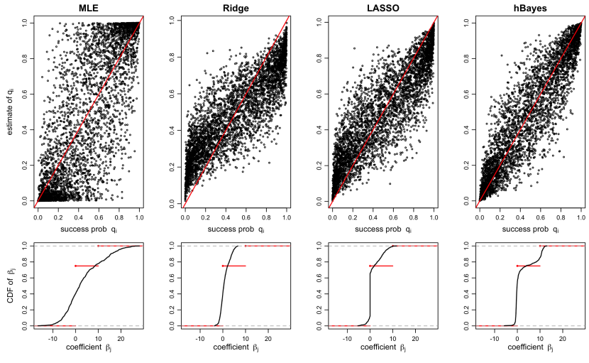
Figure 1: Estimates of the success probabilities $q_{i}$ in a logistic model.

The methodology is intended to be the primary contribution here, but we also provide some theoretical justification for the proposed method in the frequentist setup considered. Specifically, we motivate our hierarchical method as pursuing an oracle Bayes rule that uses the particular prior which assigns equal probability to every permutation of the true (and fixed) coefficient vector $\bm{\beta}$. While this is not an i.i.d. prior as in (5), only exchangeable, it is expected to differ from the product of its marginals only by a small amount when $p$ is large, because this is just the difference between sampling the $\beta_{j}$’s from their empirical distribution with versus without replacement. Indeed, for compound decision problems, which consist of $n$ independent copies of the same marginal problem to be solved under the sum of the individual losses, Hannan and Robbins (1955) and Greenshtein and Ritov (2009) have proved asymptotic equivalence of the corresponding frequentist risks, under some mild conditions. Taking the aforementioned oracle Bayes rule as the target for our hierarchical method, in Section 2 we turn the focus to this oracle Bayes rule itself, and show in both the orignal frequentist setup and a Bayes setup, that it has some (non-asymptotic) instance-optimality properties, meaning optimality for the vector $\bm{\beta}$ that actually happens to underlie the measurements.

The remaining sections of the paper are organized as follows. Section 3 reviews finite Polya tree priors and describes our Gibbs algorithm for posterior inference in GLMs. A simulation for a logistic regression model is presented in Section 4, and a real data application in genetic association studies is presented in Section 5. Section 6 concludes with a discussion and directions for future research.

2 Oracle shrinkage rules

Before presenting the details for our hierarchical method, in this section we give some theoretical support for the proposed approach. As pointed out earlier, the proposed hierarchical Bayes approach is generally intended to produce similar results to a nonparametric EB approach. Thus, our purpose in this section is to provide formal justification for regarding the coefficients as random,

$$\beta_{j}\stackrel{{\scriptstyle iid}}{{\sim}}\bar{\pi},\ \ \ \ \ \ \ \bar{\pi}\ \text{unknown},$$ (7)

even when $\beta_{j}$ in the model (1) are in fact fixed. To do this, we show that the Bayes rule under the particular prior which assigns equal probability to every permutation of $\bm{\beta}$, is, in some sense, an optimal shrinkage estimator also when $\bm{\beta}$ is fixed; once this is established, the modeling above will be justified because, as we explain later, an empirical Bayes rule under (7) is a good approximation of the aforementioned optimal rule. We say “in some sense” when referring an optimal shrinker, first because the Bayes rule under the particular prior mentioned above is not a legal estimator, rather an oracle, as it depends on the unknown $\bm{\beta}$; and secondly, because we do put some restriction on the estimator when searching for a best one. The two points in this clause are related: if we leave open the option to use the true vector $\bm{\beta}$ in choosing an estimator, then, without any restrictions, the trivial estimator $\hat{\bm{\beta}}\equiv\bm{\beta}$ usually attains minimum risk (in fact, minimum loss), and cannot be improved. However, if we somehow restrict the class of estimators, then even with full knowledge of $\bm{\beta}$, the oracle—the best rule in the restricted class—becomes nontrivial, because $\hat{\bm{\beta}}\equiv\bm{\beta}$ is generally excluded from the class under consideration. The situation is most interesting when the restriction is mild enough to include sensible estimators for the problem, but still sufficiently binding so that the risk of the oracle can be asymptotically approached by a legal (depending only on the data) estimator. This is the essence of Robbins’s “competitive” approach for compound decision problems, which we review below.

For simplicity, we will assume throughout this section that the nuisance parameter $\psi$ is fixed and known; the arguments that follow can be adapted to the case of unknown $\psi$, but we avoid this so as not to distract from the main ideas. With this assumption, the given model (1) has the general form

$$Y_{i}\stackrel{{\scriptstyle ind}}{{\sim}}f_{i}(y_{i};\bm{\beta}),\ \ \ \ \ i=1,...,n,$$ (8)

and the the task is to estimate the fixed vector $\bm{\beta}$ under a given loss function $L(\bm{\beta},\hat{\bm{\beta}})$. For any estimator $\delta(\bm{y})$, where $\delta:\mathbb{R}^{n}\to\mathbb{R}^{p}$, the risk is $R(\bm{\beta},\delta)=\mathbb{E}_{\bm{\beta}}L(\bm{\beta},\delta(\bm{Y}))$, considered as a function of $\bm{\beta}$.

2.1 Review: Robbins’s compound decision theory

In some special cases of the setup descrived above, the “competitive” approach referred to earlier turns out to be very successful, as demonstrated by Robbins (starting with Robbins, 1951). Robbins considered compound decision problems, entailing a separable model,

$$Y_{j}\stackrel{{\scriptstyle ind}}{{\sim}}f(y_{j};\beta_{j}),\ \ \ \ \ j=1,...,p,$$ (9)

and a loss function of the additive form $L(\bm{\beta},\hat{\bm{\beta}})=\sum_{j}\bar{L}(\beta_{j},\hat{\beta}_{j})$, where $\bar{L}(\beta,\hat{\beta})$ is any “marginal” loss function. Note that this is a specialization of the model (8) and the loss function $L(\bm{\beta},\hat{\bm{\beta}})$. Rather than the popular approach of seeking a minimax estimator, which gives only worst-case optimality guarantee, Robbins pursued estimators $\delta$ with the property that, under certain regularity conditions,

$$R(\bm{\beta},\delta)-R(\bm{\beta},\delta^{*})\to 0\ \ \text{as }p\to\infty,\ \ \ \ \ \ \ \text{for }\textit{all }\bm{\beta},$$ (10)

where $\delta^{*}:=\operatorname*{arg\,min}_{\delta\in\mathcal{D}}R(\bm{\beta},\delta)$ is the oracle rule with respect to a pre-specified class $\mathcal{D}$ of estimators (note that $\delta^{*}$ depends on $\bm{\beta}$, while $\delta$ does not). Although an asymptotic property, (10) is a much stronger guarantee than minimaxity because it says that the risk of the best decision for the actual (fixed and unknown) instance $\bm{\beta}$ is attainable in the large-sample limit. Of course, (10) is interesting only if $\mathcal{D}$ is rich enough so it includes plausible estimators. That $\mathcal{D}$ cannot be the set of all estimators for (10) to hold, should be obvious because in that case the trivial rule $\delta^{*}(\bm{y})\equiv\bm{\beta}$ has zero risk, and no single estimator can approach this uniformly in $\bm{\beta}$, even asymptotically. However, a very reasonable choice of $\mathcal{D}$ can be made by appealing to invariance considerations: because the model (9) and the loss are both permutation invariant (PI), meaning essentially that relabeling the pairs $(\beta_{j},Y_{j})$ leaves the problem unchanged, it is natural to consider only estimators that are themselves PI, i.e. satisfy $\delta(\tau(\bm{y}))=\tau(\delta(\bm{y}))$ for any permutation $\tau$. As it turns out, under (9) and assuming some suitable regularity conditions, there exists $\delta$ for which (10) holds w.r.t. $\mathcal{D}^{PI}=\{\text{all PI estimators}\}$. In fact, such an estimator $\delta$ can be obtained through Robbins’s (nonparametric) EB approach, postulating (7) and estimating the corresponding Bayes rule from the data.

The key to understanding why the EB formulation is suitable for the frequentist problem, is the observations Robbins made about the oracle rule itself. In what follows, since we will be considering Bayes models with (oracle) priors that depend on the true and fixed $\bm{\beta}$, we shall use $\bm{b}$ to denote a random coefficient vector. Thus, Hannan and Robbins (1955) show that the oracle PI rule in a compound decision problem, is in fact the Bayes rule in the pretended two-level model

$$\bm{b}\sim\pi^{*}$$ (11)

$$Y_{j}\lvert b_{j}\stackrel{{\scriptstyle ind}}{{\sim}}f(y_{j};b_{j}),$$

where $\pi^{*}$ denotes the uniform prior on all $p!$ permutations of $\bm{\beta}$ (i.e., the distribution resulting from drawing a permutation $\tau\in S_{n}$ uniformly at random, then applying $\tau$ to the fixed vector $\bm{\beta}$). Importantly, note that this Bayes rule depends on $\bm{\beta}$ (because $\pi^{*}$ does), but only through its order statistic $\bar{\bm{\beta}}=(\bar{\beta}_{1},...,\bar{\beta}_{p})=(\beta_{(1)}\leq\beta_{(2)}\leq\cdots\leq\beta_{(p)})$. To emphasize this, we denote the oracle PI rule by

$$\delta^{*}(\bm{y};\bar{\bm{\beta}}):=\arg\min_{\mathbf{a}\in\mathbb{R}^{p}}\mathbb{E}_{\bar{\bm{\beta}}}[L(\bm{b},\mathbf{a})\lvert\bm{Y}=\bm{y}],$$ (12)

where, by convention, $\mathbb{E}_{\bar{\bm{\beta}}}[\cdot]$ denotes expectation under (11).

While the prior used by the oracle is not i.i.d. for any finite $p$, when $p\to\infty$ it is intuitively expected, by De Finetti-type results, to converge in some sense to the i.i.d. product of its marginals; see Diaconis and Freedman (1980) regarding the difference between sampling with and without replacement. Therefore, the oracle PI estimator of $\bm{\beta}$ is expected to be asymptotically equivalent to the Bayes rule under

$$b_{j}\stackrel{{\scriptstyle iid}}{{\sim}}\bar{\pi}^{*}$$ (13)

$$Y_{j}\lvert b_{j}\stackrel{{\scriptstyle ind}}{{\sim}}f(y_{j};b_{j}),$$

where $\bar{\pi}^{*}$ is the marginal distribution of (each of) $b_{j}$ under $\bm{b}\sim\pi^{*}$. Now, it is a fact (Robbins, 1951) that the Bayes rule under (13) is the oracle simple rule, the minimizer of the risk among all rules in $\mathcal{D}^{S}=\{\delta:\delta_{j}(\bm{y})=t(y_{j})\ \text{for some function }t\}$. To summarize, the oracle PI rule is Bayes against $\bm{b}\sim\pi^{*}$, and the oracle simple rule is Bayes against $\bm{b}\sim\bar{\pi}^{*}\times\cdots\times\bar{\pi}^{*}$ ($p$ times). Asymptotic equivalence of the risks of the oracle PI rule and the oracle simple rule, is formalized and proved, under appropriate regularity conditions, in the important works of Hannan and Robbins (1955), for a hypothesis testing compound decision problem, and Greenshtein and Ritov (2009), for a point estimation compound decision problem. Now that the oracle PI estimator can be taken roughly as the Bayes rule w.r.t. the prior in (13), proceeding under the empirical Bayes formulation (7) arises naturally as a strategy for estimating the PI oracle.

2.2 An extension in the linear model

The arguments in the previous subsection rely crucially on permutation invariance of the model (9). If we want to speak of permutation invariance under the (much) more general model (8), in particular for a GLM, we first need to think how to define it. In the separable model (9), permutation invariance formally means that the distribution of $\bm{Y}$ under a permutation $\bm{\beta}^{\prime}=\tau(\bm{\beta})$ is the same as the distribution of $\bm{Y}^{\prime}=\tau(\bm{Y})$ under $\bm{\beta}$. This definition is not even applicable in a GLM, because in (1) the dimensions of $\bm{Y}$ and $\bm{\beta}$ are not the same. Still, in some special cases, the situation can be reduced through sufficiency to a simpler model, where we can identify the conditions for permutation invariance using the usual definition. Importantly, even though the reduction will not recover the model (9) exactly, we will see that Robbins’s arguments continue to hold, and in fact imply that the oracle PI rule in that case uses the same oracle prior $\pi^{*}$. This will justify the modeling in (7) beyond the separable model, thereby extending the theory reviewed in the previous subsection.

We first extend the definition of the oracle rule (12) beyond the separable model. Thus, consider the postulated Bayes model

$$\bm{b}\sim\pi^{*}$$ (14)

$$\bm{Y}\lvert\bm{b}\sim f(\bm{y};\bm{X}\bm{b},\psi),$$

where $f(\bm{y};\bm{\eta},\psi)$ is the likelihood in (1), and recall that $\pi^{*}$ depends on $\bm{\beta}$ through $\bar{\bm{\beta}}$. We define the oracle Bayes rule for the (frequentist) model (1) to be the Bayes rule under (14), that is,

$$\delta^{*}(\bm{y};\bar{\bm{\beta}})=\operatorname*{arg\,min}_{\mathbf{a}\in\mathbb{R}^{p}}\mathbb{E}_{\bar{\bm{\beta}}}[L(\bm{b},\mathbf{a})\lvert\bm{Y}=\bm{y}].$$ (15)

Note that this indeed extends the definition of (12), but we do not call (14) an oracle PI rule because, as explained above, it is not clear what permutation invariance (and hence a PI rule) would mean under (1).

We now restrict attention to the special case of the linear model (2), and remember that we regard $\sigma^{2}$ as known. Following the general approach proposed in, e.g., Giri (1996), instead of trying to define invariance in the original model, we will study invariance of a sufficient statistic. Thus, assuming that $\bm{X}$ has full column rank (otherwise $\bm{\beta}$ is not identifiable), we first replace (2) by the likelihood of the least squares (LS) estimator,

$$\mathbf{Z}=(\bm{X}^{\top}\bm{X})^{-1}\bm{X}^{\top}\bm{Y}\sim\mathcal{N}_{p}(\bm{\beta},\sigma^{2}(\bm{X}^{\top}\bm{X})^{-1}).$$ (16)

Conveniently, $\mathbf{Z}=(Z_{1},...,Z_{p})^{\top}$ has the same dimension as the parameter $\bm{\beta}$, and, moreover, the marginal distribution of $Z_{j}$ depends only on $\beta_{j}$. The statistic $\mathbf{Z}$ still does not follow the separable model (9), because the components $Z_{j}$ are not independent. However, suppose that for some $-1\leq\rho\leq 1$,

$$\bm{X}^{\top}\bm{X}\propto\left[\begin{array}[]{ccccc}1&\rho&\rho&\cdots&\rho\\ \rho&1&\rho&\cdots&\rho\\ \rho&\rho&1&\cdots&\rho\\ \vdots&\vdots&\vdots&\ddots&\vdots\\ \rho&\rho&\rho&\cdots&1\end{array}\right].$$ (17)

In that case we can represent

$$\mathbf{Z}\stackrel{{\scriptstyle d}}{{=}}\bm{\beta}+\bm{\epsilon}$$

where $\bm{\epsilon}=(\epsilon_{1},...,\epsilon_{p})$ is a zero-mean, exchangeable random vector. It then obviously still holds that the distribution of $\mathbf{Z}$ under a permutation $\bm{\beta}^{\prime}=\tau(\bm{\beta})$ is the same as the distribution of $\mathbf{Z}^{\prime}=\tau(\mathbf{Z})$ under $\bm{\beta}$. In other words, the model (16) is PI by the standard definition, and, correspondingly, we can look for an oracle PI rule in terms of $\mathbf{Z}$. The following proposition says that, under (17), the oracle PI rule in $\mathbf{Z}$ coincides with the oracle Bayes rule (15).

Proposition 1.

In the linear model (2) with known $\sigma^{2}$, consider estimating $\bm{\beta}$ from the sufficient statistic $\mathbf{Z}$, and assume that the loss function is PI, that is, $L(\bm{\beta},\hat{\bm{\beta}})=L(\tau(\bm{\beta}),\tau(\hat{\bm{\beta}}))$ for every permutation $\tau$. Suppose that the $\bm{X}$ matrix has the form (17), so that the model for $\mathbf{Z}$ is PI, and let $\delta^{*}(\mathbf{z};\bar{\bm{\beta}})$ be the minimizer of the risk of over all PI rules $\delta(\mathbf{z})$. Then, if $\delta^{*}(\bm{y};\bar{\bm{\beta}})$ is the oracle Bayes rule (15), we have $\delta^{*}(\bm{y};\bar{\bm{\beta}})=\delta^{*}(\mathbf{z};\bar{\bm{\beta}})$.

Proof.

Let $\delta(\mathbf{z})$ be a PI rule under the PI model (16). Then we can proceed as in Weinstein (2021) and calculate the risk of $\delta$ at $\bm{\beta}$,

$$R(\bm{\beta},\delta) =\mathbb{E}_{\bm{\beta}}L(\bm{\beta},\delta(\mathbf{Z}))$$ (18)

$$=\mathbb{E}_{\bm{\beta}}L(\tau(\bm{\beta}),\tau(\delta(\mathbf{Z})))$$

$$=\mathbb{E}_{\bm{\beta}}L(\tau(\bm{\beta}),\delta(\tau(\mathbf{Z})))$$

$$=\mathbb{E}_{\tau(\bm{\beta})}L(\tau(\bm{\beta}),\delta(\mathbf{Z}))$$

$$=R(\tau(\bm{\beta}),\delta),$$

where the subscript on the expectation operator is the value of the parameter indexing the distribution of $\mathbf{Z}$, not of $\tau(\mathbf{Z})$. Above, the second equality is because the loss is PI, the third equality is because the rule $\delta$ is PI, and, crucially, the fourth inequality is because the model for $\mathbf{Z}$ is PI under (17). Now, since Equation (18) says that, for a PI rule $\delta$, the risk is constant on permutations of $\bm{\beta}$, it follows that

$$R(\bm{\beta},\delta)=\frac{1}{p!}\sum_{\tau}R(\tau(\bm{\beta}),\delta),$$

the sum taken over all $p!$ permutations $\tau$. This is precisely the Bayes risk of $\delta$ under a pretended Bayes model where

$$\bm{b}\sim\pi^{*}$$ (19)

$$\mathbf{Z}\lvert\bm{b}\sim\mathcal{N}_{p}(\bm{b},\sigma^{2}(\bm{X}^{\top}\bm{X})^{-1}).$$

But this is also the Bayes rule under (14), because $\mathbf{Z}$ is a sufficient statistic. ∎

The methodology to be presented in Section 3 can be used for estimating the oracle Bayes rule (14), in fact, they do so without assumptions on $\bm{X}$ and apply to GLMs, not only linear models. One important simplification which we allow ourselves to use in motivating our methods, is that, as in the compound decision case (where such results have been established formally), the Bayes rule under (14) is expected again to be asymptotically equivalent to the Bayes rule on replacing $\pi^{*}$ with the product prior $\bar{\pi}^{*}\times\cdots\times\bar{\pi}^{*}$ ($p$ times). In any case, we note that the usual deconvolution EB methods are not appropriate, because these are designed for the separable case (9); if reduction to $\mathbf{Z}$ in (16) is carried out, then $Z_{j}$ are generally not independent, even under the assumption (17). The methods in Section 3 take such dependencies into account when estimating the empirical distribution of the parameters $\beta_{j}$.

2.3 Bayes optimality for GLMs

The extension in the last subsection applies in the special case of a linear model and under some further conditions on the matrix $\bm{X}$. Otherwise, the model in the general case (1) is not necessarily PI (under any sensible definition of permutation invariance), and the modeling (7) might not have as strong a frequentist justification. However, even in the general case (1) with an arbitrary $\bm{X}$, it still seems reasonable, as proposed in Lindley and Smith (1972), to assume an exchangeable prior on $\bm{\beta}$. In other words, to consider a genuinely Bayesian model,

$$\bm{\beta}\ \sim\ \pi$$ (20)

$$\bm{Y}\lvert\bm{\beta}\sim f(\bm{y};\bm{\eta},\psi)$$

where $f(\bm{y};\bm{\eta},\psi)$ is the likelihood in (1), and where the prior $\pi$ is such that $\pi(\bm{\beta})=\pi(\tau(\bm{\beta}))$ for every permutation $\tau$, but otherwise completely unknown. Note that, to distinguish from the frequentist setting where the prior was pretended rather than assumed part of the model, we use here $\bm{\beta}$ instead of $\bm{b}$. In Lindley and Smith (1972) fully-specified, gaussian priors are used for $\bm{\beta}$, and, although connections to frequentist results in the style of Stein’s estimator are pointed out, they declare at the outset that “the argument is entirely within the Bayesian framework”. By contrast, here we do not assume anything about $\pi$ except for exchangeability, hence the results below will still have a strong frequentist flavor: in essence, we show that, if $\pi$ is exchangeable, then the oracle Bayes rule (15) always yields smaller Bayes risk than the (standard) Bayes rule under (20). In other words, there is a rule which does not depend on $\pi$ and yet is better than the Bayes rule under (20). This will be possible because the ordinary Bayes rule w.r.t. $\pi$, as usual, has access to $\pi$ but not $\bm{\beta}$, whereas our oracle Bayes rule will depend on $\bm{\beta}$ through $\bar{\bm{\beta}}$ (but not on $\pi$).

To formalize this statement, we first observe that for any prior $\pi$, not necessarily exchangeable, the Bayes estimator that has access to $\bar{\bm{\beta}}$ in addition to $\bm{Y}$ is, quite trivially, at least as good as the Bayes estimator that only sees $\bm{Y}$. In other words, for any loss function $L(\bm{\beta},\hat{\bm{\beta}})$, we have

$$\min_{{\delta}}\mathbb{E}_{\pi}[L(\bm{\beta},\delta(\bm{Y},\bar{\bm{\beta}}))]\leq\min_{\delta}\mathbb{E}_{\pi}[L(\bm{\beta},\delta(\bm{Y}))],$$ (21)

where on the left hand side the minimum is over all functions $\delta$ of $(\bm{y},\bar{\bm{\beta}})$, and on the right hand side the minimum is over all functions $\delta$ of $\bm{y}$; and where in both sides of the inequality the expectation $\mathbb{E}_{\pi}[\cdot]$ is with respect to the joint distribution of $(\bm{Y},\bm{\beta})$ under (20). Indeed, since any function of $\bm{Y}$ only is also a function of $(\bm{Y},\bar{\bm{\beta}})$, the minimum on the left hand side of (21) is taken over a larger set of rules, implying the inequality.

The following proposition says that, if $\pi$ is an exchangeable prior, the oracle Bayes rule (15) outperforms the Bayes rule in $\bm{Y}$ under $\pi$. As we show below, while the latter generally depends on $\pi$, for exchangeable $\pi$ this dependence goes away once conditioning on the order statistic $\bar{\bm{\beta}}$.

Proposition 2.

If $\pi$ is exchangeable, then the rule (15) attains the minimum on the left hand side of (21).

Proof.

It is enough to show that for any realization $(\bm{y},\bar{\bm{\beta}})$ of $(\bm{Y},\bar{\bm{\beta}})$,

$$\operatorname*{arg\,min}_{\mathbf{a}\in\mathbb{R}^{p}}\mathbb{E}_{\pi}[L(\bm{\beta},\mathbf{a})\lvert\bar{\bm{\beta}},\bm{Y}=\bm{y}]=\operatorname*{arg\,min}_{\mathbf{a}\in\mathbb{R}^{p}}\mathbb{E}_{\bar{\bm{\beta}}}[L(\bm{b},\mathbf{a})\lvert\bm{Y}=\bm{y}],$$ (22)

where $\mathbb{E}_{\pi}[\cdot]$ is expectation w.r.t. (20), and $\mathbb{E}_{\bar{\bm{\beta}}}[\cdot]$ is expectation w.r.t. (14). Now, the left hand side above is the Bayes rule in $(\bm{Y},\bar{\bm{\beta}})$, i.e., the action $\mathbf{a}\in\mathbb{R}^{p}$ that minimizes the posterior expected loss w.r.t. the conditional distribution of $\bm{\beta}$ given $\bar{\bm{\beta}}$ and $\bm{Y}=\bm{y}$. Note that this posterior is supported on the set of all permutations $\tau(\bar{\bm{\beta}})$ of $\bar{\bm{\beta}}$. Calculating the posterior for any particular value $\bm{\beta}$, say $\bm{\beta}=\tau(\bar{\bm{\beta}})$ for some permutation $\tau$, we have

$$\pi(\bm{\beta}|\bm{y},\bar{\bm{\beta}})\propto\pi(\bm{\beta}|\bar{\bm{\beta}})f(\bm{y}|\bm{\beta},\bar{\bm{\beta}})=\pi(\bm{\beta}|\bar{\bm{\beta}})f(\bm{y}|\bm{\beta}),$$ (23)

and

$$\pi(\bm{\beta}|\bar{\bm{\beta}})=\pi(\tau(\bar{\bm{\beta}})|\bar{\bm{\beta}})\propto\pi(\tau(\bar{\bm{\beta}})).$$ (24)

Now, since $\pi$ is assumed to be exchangeable, (24) does not depend on $\tau$, in other words, we have $\pi(\bm{\beta}|\bar{\bm{\beta}})=\pi^{*}(\bm{\beta})$. Replacing this in (23) gives

$$\pi(\bm{\beta}|\bm{y},\bar{\bm{\beta}})\propto\pi^{*}(\bm{\beta})f(\bm{y}|\bm{\beta}).$$

implying that the posterior of $\bm{\beta}$ given $\bar{\bm{\beta}}$ and $\bm{Y}=\bm{y}$, is equal to the posterior of $\bm{\beta}$ under the Bayes model where the prior is $\pi^{*}$ and the likelihood is (1). But this is exactly the distribution of $\bm{b}$ under which the expectation on the right hand side of (22) is calculated. ∎

3 Hierarchical Bayes modeling for high-dimensional GLMs

Assuming (1) with $\bm{\beta}$ fixed, the previous section advances an oracle prior, under which $\beta_{j}$ are i.i.d. from the empirical distribution of the coordinates $\bar{\beta}_{1},...,\bar{\beta}_{p}$ of $\bar{\bm{\beta}}$. We now describe a hierarchical Bayes model which postulates that the parameter vector has been generated from a Polya tree prior. Intuitively, we expect the posterior distribution of the parameter vector in the postulated hierarchical model to implicitly learn the empirical distribution of the components of the true (fixed) $\bm{\beta}$, thereby yielding Bayes rules that mimic oracle Bayes rules.

As usual, in this hierarchical generative model, the likelihood from (1) is treated as the conditional distribution $f(\bm{y}|\bm{X}\bm{\beta},\psi)$ of $\bm{Y}$ given $\bm{\beta}$ and $\psi$. At the second level, conditionally on a random univariate distribution $\bar{\Pi}=\bar{\pi}$, the parameters $\bm{\beta}$ and $\psi$ are taken to be independent, where $\beta_{j}\sim\bar{\pi}$, i.i.d., and where $\psi\sim f(\psi)$ is a noninformative prior on the nuisance parameter. At the third level, $\bar{\pi}$ is modeled as a finite Polya tree.

The finite Polya tree model. The $L$-level finite Polya tree (FPT) model generates distributions with piecewise constant density functions on a dyadic partition of ${\cal I}_{0}=(a_{min},a_{\max}]$, corresponding to a fixed endpoints vector $\bm{\mathrm{a}}:=(a_{min}=a_{0}\leq a_{1}\leq\cdots\leq a_{2^{L}-1}\leq a_{2^{L}}=a_{max})$. The dyadic partition consists of subintervals ${\cal I}_{l,i}=(a_{(i-1)\cdot 2^{L-l}},a_{i\cdot 2^{L-l}}]$, for $l=1\cdots L$ and $i=1\cdots 2^{l}$. The parameters of the FPT model are the Beta hyper-parameters $(\alpha_{l,i},\beta_{l,i})$, corresponding to subintervals ${\cal I}_{l-1,i}$ for $l=1\cdots L$ and $i=1\cdots 2^{l-1}$. The FPT model is described by the following components.

• Independent Beta random variables. A vector ${\bm{\mathrm{\phi}}}=(\phi_{1,1}\cdots\phi_{L,2^{L-1}})$ of independent Beta random variables $\phi_{l,i}\sim Beta(\alpha_{l,i},\beta_{l,i})$, specifying conditional subinterval probabilities for the dyadic partition. Specifically, $\mathbb{P}({\cal I}_{1,1}|{\cal I}_{0})=\phi_{1,1}$ and $\mathbb{P}({\cal I}_{1,2}|{\cal I}_{0})=1-\phi_{1,1}$, and, for $l=2\cdots L$ and $i=1\cdots 2^{l-1}$, $\mathbb{P}({\cal I}_{l,2\cdot i-1}|{\cal I}_{l-1,i})=\phi_{l,i}$ and $\mathbb{P}({\cal I}_{l,2\cdot i}|{\cal I}_{l-1,i})=1-\phi_{l,i}$.

• Subinterval probabilities. The subinterval probabilities vector $\bm{\mathrm{\pi}}$ has elements $\mathbb{P}({\cal I}_{l,i})=\pi_{l,i}$, which are products of the conditional subinterval probabilities, that is, $\pi_{1,1}=\phi_{1,1}$ and $\pi_{1,2}=1-\phi_{1,1}$, and, for $l=2\cdots L$ and $i=1\cdots 2^{l-1}$, $\pi_{l,2\cdot i-1}=\phi_{l,i}\cdot\pi_{l-1,i}$ and $\pi_{l,2\cdot i}=(1-\phi_{l,i})\cdot\pi_{l-1,i}$.

• Step function PDF. The step function density is specified by the vector $\bm{\mathrm{\pi}}_{L}=(\pi_{L,1}\cdots\pi_{L,2^{L}})$ of subinterval probabilities for level $L$,

  $$\bar{\pi}(\beta|\bm{\mathrm{\pi}}_{L})=\pi_{L,1}\cdot\mathbbm{1}_{L,1}(\beta)/(a_{1}-a_{0})+\cdots+\pi_{L,2^{L}}\cdot\mathbbm{1}_{L,2^{L}}(\beta)/(a_{2^{L}}-a_{2^{L}-1}),$$ (25)

  for $\beta\in{\cal I}_{0}$, where $\mathbbm{1}_{L,i}(\beta)$ is the indicator function corresponding to ${\cal I}_{L,i}$.

We provide posterior inference assuming that the observed data $\bm{Y}$ is a realization from the following generative model:

1. Generate ${\psi}\sim f({\psi})$.

2. Generate $\bar{\pi}(\cdot|\bm{\mathrm{\pi}}_{L})$ from the FPT model with $\phi_{l,i}\sim Beta(1,1)$.

3. Given $\bm{\mathrm{\pi}}_{L}$, generate $\bm{\mathrm{\beta}}=(\beta_{1}\cdots\beta_{p})$, with $\beta_{j}\sim\bar{\pi}(\beta|\bm{\mathrm{\pi}}_{L})$, i.i.d., for $j=1\cdots p$.

4. Given $\bm{\beta}$ and $\psi$, generate $\bm{\mathrm{Y}}$ from $p\left({\bm{\mathrm{y}}}|{\bm{\mathrm{\beta}}},\psi\right)=f(\bm{y};\bm{X}\bm{\beta},\psi)$.

Setting the FPT model parameters $(\alpha_{l,i},\beta_{l,i})$ in the generative model to $1$ makes the prior marginal distribution of $\beta_{j}$ the uniform density on $[a_{min},a_{max}]$, and expresses large prior uncertainty regarding the distribution of the subinterval probabilities. Denoting ${\bm{\mathrm{\Theta}}}=\{\psi,{\bm{\mathrm{\beta}}},{\bm{\mathrm{\phi}}}\}$, our estimates are Bayes rules based on the posterior distribution of ${\bm{\mathrm{\Theta}}}$ given $\bm{\mathrm{Y}}={\bm{\mathrm{y}}}$ under the generative model. That is,

$$p(\psi,{\bm{\mathrm{\beta}}},{\bm{\mathrm{\phi}}}|{\bm{\mathrm{y}}})=\frac{p({\bm{\mathrm{\phi}}}|\psi,\bm{\mathrm{\beta}},{\bm{\mathrm{y}}})p(\psi|\bm{\mathrm{\beta}},{\bm{\mathrm{y}}})p(\bm{\mathrm{\beta}}|{\bm{\mathrm{y}}})p({\bm{\mathrm{y}}})}{p({\bm{\mathrm{y}}})}=p(\bm{\mathrm{\phi}}|\bm{\mathrm{\beta}})\pi(\psi|\bm{\mathrm{\beta}},{\bm{\mathrm{y}}})p(\bm{\mathrm{\beta}}|{\bm{\mathrm{y}}}).$$ (26)

Now let $N_{l,i}=N_{l,i}(\bm{\beta})=|\{j:\beta_{j}\in{\cal I}_{l,i}\}|$ and let ${\bm{\mathrm{N}}}=(N_{1,1},...,N_{L,2^{L}})$. Ferguson (1974) has already noted the conjugacy of the FPT model, namely, that the conditional distribution of $\bm{\mathrm{\phi}}$ given ${\bm{\mathrm{N}}}$, is again a FPT, now with updated hyper-parameter values,

$$\phi_{l,i}|{\bm{\mathrm{N}}}\sim Beta(1+N_{l,2\cdot i-1},1+N_{l,2\cdot i}).$$ (27)

Under the generative model we observe only $\bm{Y}$, not the latent vector $\bm{\beta}$. Noting that $p(\bm{\mathrm{\phi}}|\bm{\mathrm{\beta}})$ is the FPT model in (27), (26) reveals that the posterior of $\bm{\mathrm{\phi}}$ is a FPT mixture. Meanwhile, $p(\psi|\bm{\mathrm{\beta}},{\bm{\mathrm{y}}})$ depends on the likelihood and the prior on $\psi$. E.g., for the Normal linear model and an inverse chi-squared prior, $p(\psi|\bm{\mathrm{\beta}},{\bm{\mathrm{y}}})$ is inverse chi-squared with updated hyper-parameter values.

We evaluate the posterior distribution of ${\bm{\mathrm{\Theta}}}$ by a Gibbs sampling algorithm. Specifically, we (i) sample ${\bm{\mathrm{\beta}}}|\,\psi,{\bm{\mathrm{\phi}}},{\bm{\mathrm{y}}}$ using a single-site Metropolis Hastings (MH) algorithm that draws each component of ${\bm{\mathrm{\beta}}}$ conditional on the remaining components of ${\bm{\mathrm{\beta}}}$, as detailed in section A in the Appendix, (ii) sample ${\bm{\mathrm{\phi}}}|\,{\bm{\mathrm{\beta}}}$ from the conditional distribution (27), and (iii) sample $\psi|\,{\bm{\mathrm{\beta}}},{\bm{\mathrm{y}}}$, which is case dependent on the likelihood (1). Algorithm 1 describes the Gibbs sampling algorithm for the gaussian linear regression likelihood (2).

Set : number of Gibbs sampler iterations $G$, number of levels $L$,

endpoints vector $\bm{\mathrm{a}}$, initial values ${\bm{\mathrm{\Theta}}}^{(0)}$

Input : $\bm{\mathrm{y}}$, $\bm{\mathrm{X}}$

Output : posterior samples ${\bm{\mathrm{\Theta}}}^{(1)}\cdots,{\bm{\mathrm{\Theta}}}^{(G)}$

1

2

3for $g=1,\cdots,G$ do

4      

5      for $j=1,\cdots,p$ do

6             Sample $\beta_{j}^{(g)}|\psi^{(g-1)},{\bm{\mathrm{\phi}}}^{(g-1)},{\bm{\mathrm{y}}},(\beta^{(g)}_{1},\cdots,\beta^{(g)}_{j-1},\beta^{(g-1)}_{j+1},\cdots,\beta^{(g-1)}_{p})$ by MH

7       end for

8      

9      Sample $\bm{\mathrm{\phi}}^{(g)}|\bm{\mathrm{\beta}}^{(g)}$ from (27)

10      Sample $\psi^{(g)}|\bm{\mathrm{\beta}}^{(g)},\bm{\mathrm{y}}$ from conditional inverse chi-squared distribution

11 end for

Algorithm 1 Gibbs sampler for linear regression

4 Simulations

We turn to a simulation study that will illustrate the utility of the proposed methods. To demonstrate the applicability beyond linear regression, in this section we will focus on a logistic regression model, and compare our methods to some alternatives in terms of (empirical) estimation accuracy. We use the simulation setup of Sur and Candès (2019), where different configurations for $\bm{\beta}$ are considered, and $\bm{X}$ consists of $n=4000$ rows and $p=800$ columns of i.i.d. $\mathcal{N}(0,1/n)$ entries, with the only difference that we draw $\bm{X}$ once and keep it fixed throughout the experiment. We consider three different configurations for the coefficient vector $\bm{\beta}$:

• Scenario 1: $\bm{\beta}$ has $100$ replicates of $-10$, $100$ replicates of $+10$, and $600$ zeros.

• Scenario 2: $\bm{\beta}$ consists of $800$ i.i.d. $\mathcal{N}(3,16)$ realizations.

• Scenario 3: $\bm{\beta}$ consists of $400$ i.i.d $\mathcal{N}(7,1)$ realizations, and $400$ zeros.

For Scenario $k=1,2,3$, in each of $30$ simulation rounds we generate $\bm{Y}$ from the logistic regression likelihood (3), and measure the error in estimating $\bm{\beta}$ using $\widehat{RMSE}=\sqrt{\sum_{j=1}^{p}(\beta_{j}-\hat{\beta}_{j})^{2}/p}$. We compared six point estimators of the vector $\bm{\beta}$: the maximum likelihood estimator (“MLE”), $\hat{\bm{\beta}}^{MLE}$; the bias-corrected maximum likelihood estimator (“adj-MLE”) of Sur and Candès (2019), $\hat{\bm{\beta}}^{MLE}/1.499$; a Ridge-penalized estimator (“Ridge”) and an $\ell_{1}$-penalized estimator (“LASSO”), implemented using the cv.glmnet function from the glmnet package Friedman et al. (2010) with default specifications. The proposed hierarchical Bayes estimator (“hBayes”) using a 6-level Polya tree, with $a_{min}=\min(-24,\hat{\bm{\beta}}^{MLE}-0.5)$ and $a_{max}=\max(24,\hat{\bm{\beta}}^{MLE}+0.5)$, divided evenly into $64$ subintervals, with $500$ iterations of the Gibbs sampler using the first $100$ iterations as burn-in. In principle, for each implementation of the hBayes approach we set $[a_{min},a_{max}]$ to be slightly larger than range of the components of $\hat{\bm{\beta}}^{MLE}$. For the simulation study we set wider $[a_{min},a_{max}]$ to ensure large overlap of the support of $\bar{\pi}(\beta|\bm{\mathrm{\pi}}_{L})$ for each simulation run of each scenario. For reference, we also computed the oracle Bayes estimator (“oBayes”) given in Equation (12). Performance of the Oracle Bayes estimates was evaluated by running $500$ iterations of a permutation Gibbs sampler, described in Appendix A, using the first $100$ iterations as burn-in.

Table 1 reports the estimated RMSE, the average of $\widehat{RMSE}$ over the 30 simulation runs, for the five estimators and the oracle in each of the three scenarios. In all three scenarios the hBayes estimator yielded considerably smaller RMSE than Lasso and Ridge. As expected, hBayes still has larger error than the oracle, but its RMSE is very close to that of the oracle across all three scenarios. The approximation is specifically good in Scenario 2, where the distribution of the parameter vector is relatively easy to estimate. In Scenario 1, the Lasso estimates yield smaller RMSE than Ridge estimates, while in simulations 2 and 3 Lasso yields larger RMSE than Ridge. The smaller standard errors in Table 1, further suggest that the hBayes and oBayes yield parameter estimates that are considerably more stable than Ridge and Lasso.

	MLE	oBayes	hBayes	LASSO	Ridge	adj-MLE
Scen. 1	$5.11\ (0.06)$	$1.86\ (0.03)$	$\mathbf{1.97}\ (0.02)$	$2.53\ (0.04)$	$2.85\ (0.06)$	$3.05\ (0.03)$
Scen. 2	$5.21\ (0.06)$	$2.36\ (0.01)$	$\mathbf{2.38}\ (0.01)$	$3.09\ (0.10)$	$2.91\ (0.05)$	$3.12\ (0.03)$
Scen. 3	$5.25\ (0.07)$	$2.02\ (0.01)$	$\mathbf{2.10}\ (0.01)$	$3.06\ (0.12)$	$2.90\ (0.07)$	$3.11\ (0.03)$

Table 1: Mean RMSE for estimating the parameter vector in the three simulated examples. Numbers are based on $30$ simulation runs of each simulated example. The estimated standard error for the means is listed in parenthesis.

For each scenario $k=1,2,3$, in Figure 2 we present the empirical cumulative distribution function (CDF) of the coordinates $\beta_{1},...,\beta_{p}$ of the true vector $\bm{\beta}$, along with the empirical CDF of the coordinates $\hat{\beta}^{MLE}_{1},...,\hat{\beta}^{MLE}_{p}$ of the MLE and the $0.025$, $0.50$, $0.975$, quantiles of the posterior distribution of the CDF of $\bar{\pi}(\beta|\bm{\mathrm{\pi}}_{L})$ in the generative model, in one simulation run. In all three scenarios our hierarchical Bayes method was able to recover the overall shape of the true empirical CDF, whereas this shape is undetectable from the empirical CDF of the noisy maximum likelihood estimates. Our approach produces smoothed distribution estimates that are shrunk toward the uniform distribution. This can be seen more clearly in Scenarios 1 and 3, where the distribution of the $\beta_{j}$’s has point mass; for scenario 2, in which $\beta_{j}$ were drawn from a continuous distribution, our method yielded particularly good estimates of the true empirical CDF.

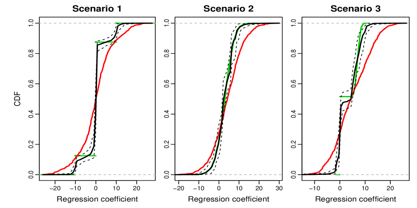
Figure 2: Estimates of the empirical CDF of the coordinates $\beta_{1},...,\beta_{p}$ of $\bm{\beta}$ for the three simulation scenarios. The green curve is the empirical CDF for $\bm{\beta}$. The red curve is the empirical CDF for the MLE. The dashed and solid black curves are the $0.025$, $0.50$ and $0.975$ quantiles of the posterior distribution of the CDF in our hierarchical Bayes analysis.

Figure 3 displays the hierarchical Bayes, Lasso and Ridge shrinkage estimates $\hat{\beta}_{j}$ in Scenario 1 versus the MLE. The grey circles in the figures correspond to the true values $\beta_{j}$, representing the ‘ideal’ shrinkage pattern. Comparing the estimates to the MLE, which would correspond to the identity line, reveals strong shrinkage for all three methods in the comparison. It is interesting to note that, since shrinkage is applied jointly to all coordinates $\hat{\beta}_{j}^{MLE},\ j=1,...,p$, the shrinkage pattern is not monotone: there exist $(j,j^{\prime})$ such that $\hat{\beta}_{j^{\prime}}^{MLE}<\hat{\beta}_{j}^{MLE}$ but $\hat{\beta}_{j^{\prime}}>\hat{\beta}_{j}$. All three shrinkage estimators yielded considerable better estimates for $\bm{\beta}$ than the maximum likelihood estimates, which had estimated RMSE of $4.97$. The Ridge estimates, which shrink the maximum likelihood estimates almost linearly, resulted in an estimated RMSE of $2.67$. The Lasso shrinkage estimates produced $323$ zero, mostly for maximum likelihood estimates lying between $-3$ and $3$; while the remaining estimates were shrunk almost linearly to $0$. The Lasso shrinkage had estimated RMSE of $2.52$. Taking the oracle as a benchmark, the hierarchical Bayes approach yielded near optimal shrinkage: estimates corresponding to MLE estimates smaller than $-12$ were shrunk to $-10$; estimates corresponding to MLE estimates between $-8$ and $8$ were shrunk to $0$; and estimates corresponding to MLE estimates larger than $12$ were shrunk to $10$. The hBayes shrinkage estimates had estimated RMSE of $2.07$. For comparison, on this particular realization the oBayes estimates yielded estimated RMSE of $2.03$

Figure 3: Shrinkage plots for Scenario 1. The horizontal axis shows the maximum likelihood estimates of $\beta_{j}$, $j=1,...,800$, and the vertical axis shows the estimate of the corresponding coefficient obtained with one of the three shrinkage methods under consideration (separate panels). Grey circles correspond to the true values $\beta_{j}$.

5 Unraveling polygenic inheritance

In this section we illustrate the application of our nonparametric Bayes approach to real data, and use our methods for unraveling the genetic architecture of polygenically inherited traits. In this context the explanatory variables are appropriately coded genotypes of genetic markers and the vector of regression coefficients represents the influence of specific genomic regions on the trait.

Many genetic studies point out that genetically inherited traits are often influenced by many genes with small effects distributed over the whole genome (Price et al., 2008; Fraser et al., 2010, 2011; Turchin et al., 2012; Visscher and Haley, 1996; Vilhjálmsson and Nordborg, 2013). As discussed e.g. in Wallin et al. (2021), analyzing the respective genetic data with the classical ”sparse” regression models leads to highly unsatisfactory results. Instead, geneticists often use mixed linear models, where the polygenic influence is captured by one random effect, summarizing the effect of all polygenes (see e.g., Kang et al. (2010)), or by many small random effects at all markers (Piepho (2009); Endelman (2011)). In the latter case the estimation of individual effects is often performed using the ridge regression, which yields the Best Linear Unbiased Predictors when the genetic effects arise from the normal distribution and the tuning parameter is adjusted to the variance of this distribution and the variance of the noise term. In Wallin et al. (2021) the classical mixed model is further extended by allowing for the nonzero mean random effect, which allows to model the situation when the investigated population is an admixture of populations which were subject to different selection pressures.

All the methods discussed above assume that the polygenic effects come from a normal distribution. As shown in the real data analysis below, this assumption might be grossly inadequate. Thus, unraveling the inheritance of polygenic traits is an interesting target for our nonparametric Bayes approach. In the following section we report the results of the simulation study and the real data analysis, which illustrate the performance of our method in the context of the analysis of such genetic data.

5.1 Simulation study

Our study follows the design of the simulation study for the experimental backcross design from Wallin et al. (2021). Thus, we simulated data for $n=400$ individuals from the backcross, where the marker genotypes can take only two values, $X_{ij}\in\{1,-1\}$, which coincide with the ancestry indictors (i.e. parental line indicators) at given loci. We simulated 10 chromosomes, each of the length of 150cM (centiMorgan), with markers spaced every 1cM. This means that for the consecutive markers on the same chromosome $P(X_{ij}=X_{i(j+1)})\approx 0.99$, while the markers on different chromosomes are independent. Following Wallin et al. (2021) the trait values are generated according to the following multiple regression model

$$\bm{Y}=\bm{X}\bm{\gamma}+\bm{X}_{m}\tilde{\bm{\beta}}+\bm{\epsilon}\;\;,$$ (28)

where $\bm{X}$ is the $400\times 1500$ incidence matrix with all marker genotypes, $\bm{\epsilon}\sim\mathcal{N}_{400}\left(\bm{0},0.1\bm{I}\right)$, and $\bm{X}_{m}$ is the $400\times 4$ matrix, whose first column consists of all ones (to model the intercept term) and the remaining three columns form a subset of $\bm{X}$ containing genotypes of markers strongly associated with the trait, $\tilde{\bm{\beta}}=(\tilde{\beta}_{0},\ldots,\tilde{\beta}_{3})\in\mathbb{R}^{4}$. The elements of the polygenic random effects vector $\bm{\gamma}=(\gamma_{1},\ldots,\gamma_{1500})$ are i.i.d. random variables from a generalized Laplace distribution, where the Normal mean-variance mixture is of the form

$$\gamma_{j}=\mu+\tau\left(\xi(V_{i}-1)+\sqrt{V_{i}}Z_{i}\right),$$

with $V_{i}\sim\Gamma(\nu,\nu)$ and $Z_{i}\sim\mathcal{N}(0,1)$. The parameter $\mu$ represents the expected value of $\gamma_{j}$, $\xi$ controls the asymmetry of the distribution, and $\nu$ the shape of the distribution. In our simulation we set $(\mu,\xi,\tau,\nu)=(-0.01,-2,0.05,0.75)$, which generates a spiked, strongly asymmetric distribution with exponential tails. Further, we set $\bm{X}_{m}=[1_{400},X_{300},X_{750},X_{1200}]$ and $\bm{\beta}=(0,0.2,0.2,-0.2)$, where the two first signals are in the opposite direction of the polygenetic effect, and the third one is in the same direction.

Figure 4 illustrates the performance of several methods for estimating large dimensional regression models on one simulated data set. Due to a very strong correlation between neighboring markers it is very difficult to appropriately estimate individual genetic effects. In our analysis we post-process the estimates provided by different methods by averaging them over $\pm$ 5cM windows within the chromosome limits. In Table 2 we also provide the estimates of the relative root mean squared error of the vector of regression coefficients $\bm{\beta}$ calculated at each position and smoothed over the 10cM window, where $\beta_{j}=\gamma_{j}$ for $j\notin\{300,750,1200\}$ and at the remaining three locations $\bm{\beta}$ is the sum of the corresponding elements of the $\bm{\gamma}$ and $\tilde{\bm{\beta}}$ vectors. The mean relative square norm (MRSN) of the error in estimating $\bm{\beta}$ is defined as $\mathbb{E}\left(\frac{||\hat{\bm{\beta}}-\bm{\beta}||}{||\bm{\beta}-\overline{\bm{\beta}}||}\right)$ where $\overline{\bm{\beta}}=\frac{1}{p}\sum_{j=1}^{p}\beta_{j}$. Additionally, we report the MRSN of the error in prediction, i.e., in estimating $\mathbb{E}(\bm{Y})=\bm{X}\bm{\beta}$. All MRSNs are estimated based on 200 independent replicates of the entire experiment, where each uses an independent draw of the design matrix $\bm{X}$, the vector of polygenic effects $\bm{\gamma}$ and the vector of error term $\bm{\epsilon}$. For each of the estimation methods considered, Figure 5 displays the distribution of the relative square norm (RSN) of the error in estimation and prediction, $||\hat{\bm{\beta}}-\bm{\beta}||\big{/}||\bm{\beta}-\overline{\bm{\beta}}||$ and $||\bm{X}(\hat{\bm{\beta}}-\bm{\beta})||\big{/}||\bm{X}(\bm{\beta}-\overline{\bm{\beta}})||$, over the 200 replicates. Additionally, in Tables 3 and 4 we report the RSN of the estimators of the three large QTL effects by the exact and smoothed versions of our estimators.

The first two panels of Figure 4 show the performance of Lasso and ridge regression, with the tuning parameters selected by the cross-validation. Panel 3 represents the results of the analysis of this dataset with the method of Wallin et al. (2021), based on the regression model (28) and assuming the normal and independent $\mathcal{N}(\mu,\tau^{2})$ prior on the distribution of polygenic effects. Large “fixed” effects QTL are identified using the forward-backward selection procedure described in Wallin et al. (2021). Finally, in the fourth panel we present the results of our nonparametric Bayes method, which does not make any assumption on the sparsity or the distribution of the regression coefficients.

Firstly, we can observe a significant difference in performance of Lasso and ridge regression. Lasso retains a rather unstable model with the variability of estimated effects substantially exceeding the variability of the true signal. By contrast, the ridge estimator substantially over-smooths the genetic signal. When averaged over 200 simulations, for Lasso the relative square norm in estimating $\bm{\beta}$ is equal to 0.89, and is smaller than RSN of ridge regression (0.96). However, the RSNs of the smoothed versions of these methods are significantly better (0.75 and 0.76) and are approximately equal to each other. Figure 5 illustrates that the exact estimates returned by ridge regression are the most stable among all considered methods. This effect, however, disappears when considering the smooth versions of other estimates. Interestingly, ridge regression performs very well in terms of prediction, with its RSN in estimating $\bm{X}\bm{\beta}$ equal to 0.02, compared to 0.07 for Lasso. We believe that this good predictive performance of ridge regression is due to the strong local correlations between marker variables, so the smoothing of the signal over neighboring positions does not harm prediction properties. However, ridge regression is not capable of accurately estimating the individual large genetic effects, with a particularly large error in estimation of the first two effects, which are in opposite direction compared to the average direction of the polygenic effects.

The mixed model approach and our nonparametric Bayes approach perform similarly. We can see that the estimates of the individual genetic effects from these two models are much more accurate than for Lasso or ridge regression. Table 3 also shows that both these methods provide much more accuracy in estimating larger QTL effects than Lasso or ridge regression. The RSN of the error in estimating $\bm{X}\bm{\beta}$ is equal to 0.02, similarly to ridge regression.

The fact that the general nonparametric Bayes approach performs as good as the dedicated mixed model of Wallin et al. (2021) in the situation when the predictors are locally strongly correlated and the signal consists both of the polygenic effects and larger fixed QTL effects, proves the versatility of the proposed approach. Moreover, Figure 6 illustrates that the nonparametric hierarchical Bayes approach picks up the the highly asymmetric distribution of the polygenic effects, which provides new insights for understanding the mode of the polygenic inheritance as compared to the classical mixed model approach, that makes the normality assumption on the polygenic effects.

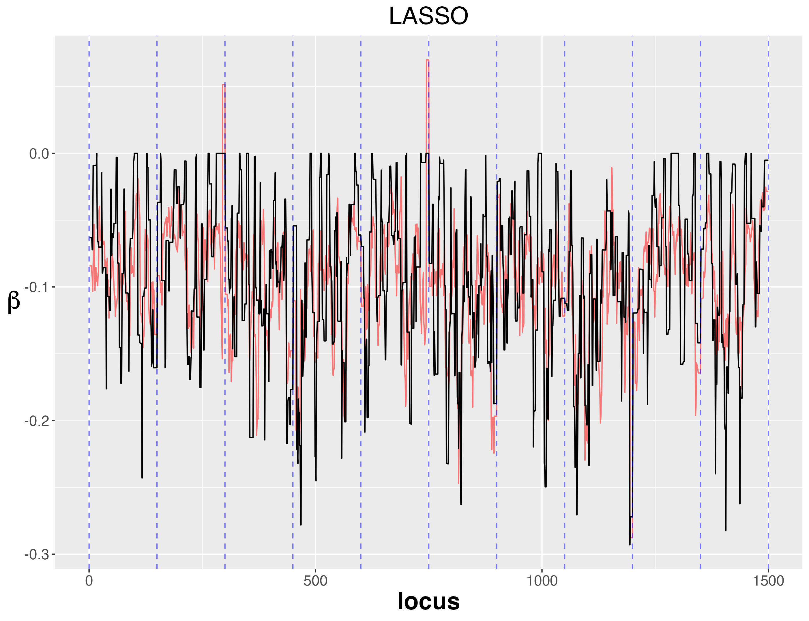
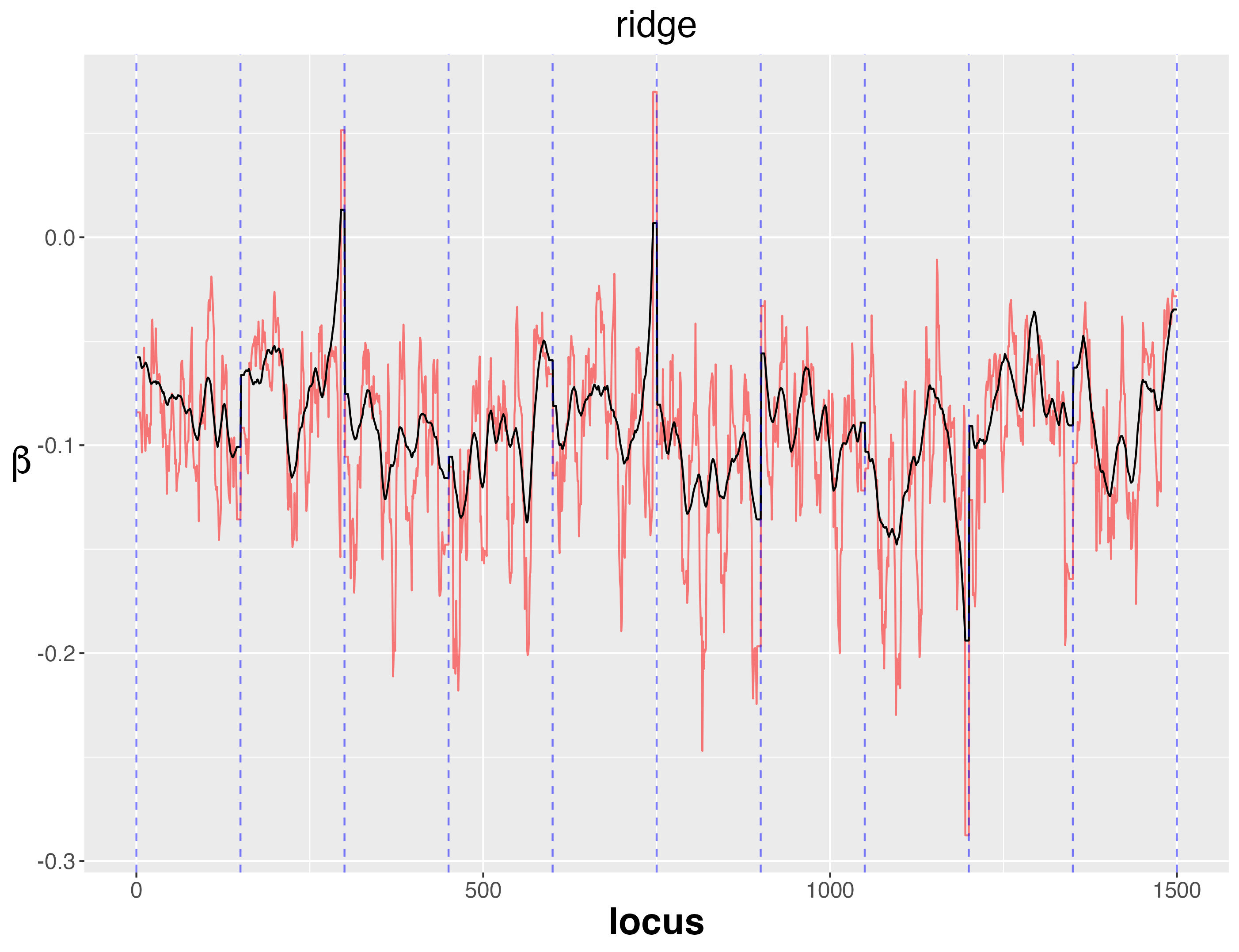
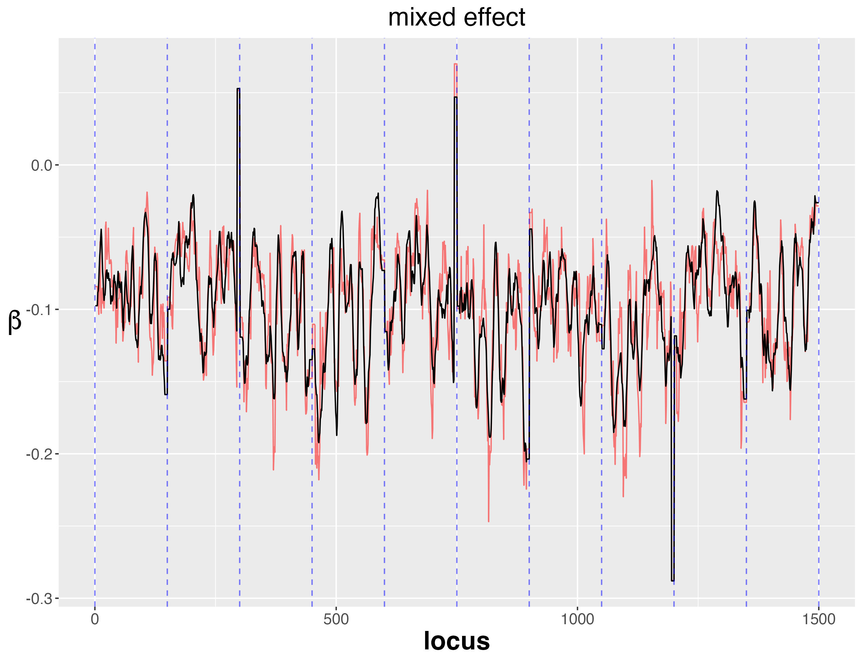
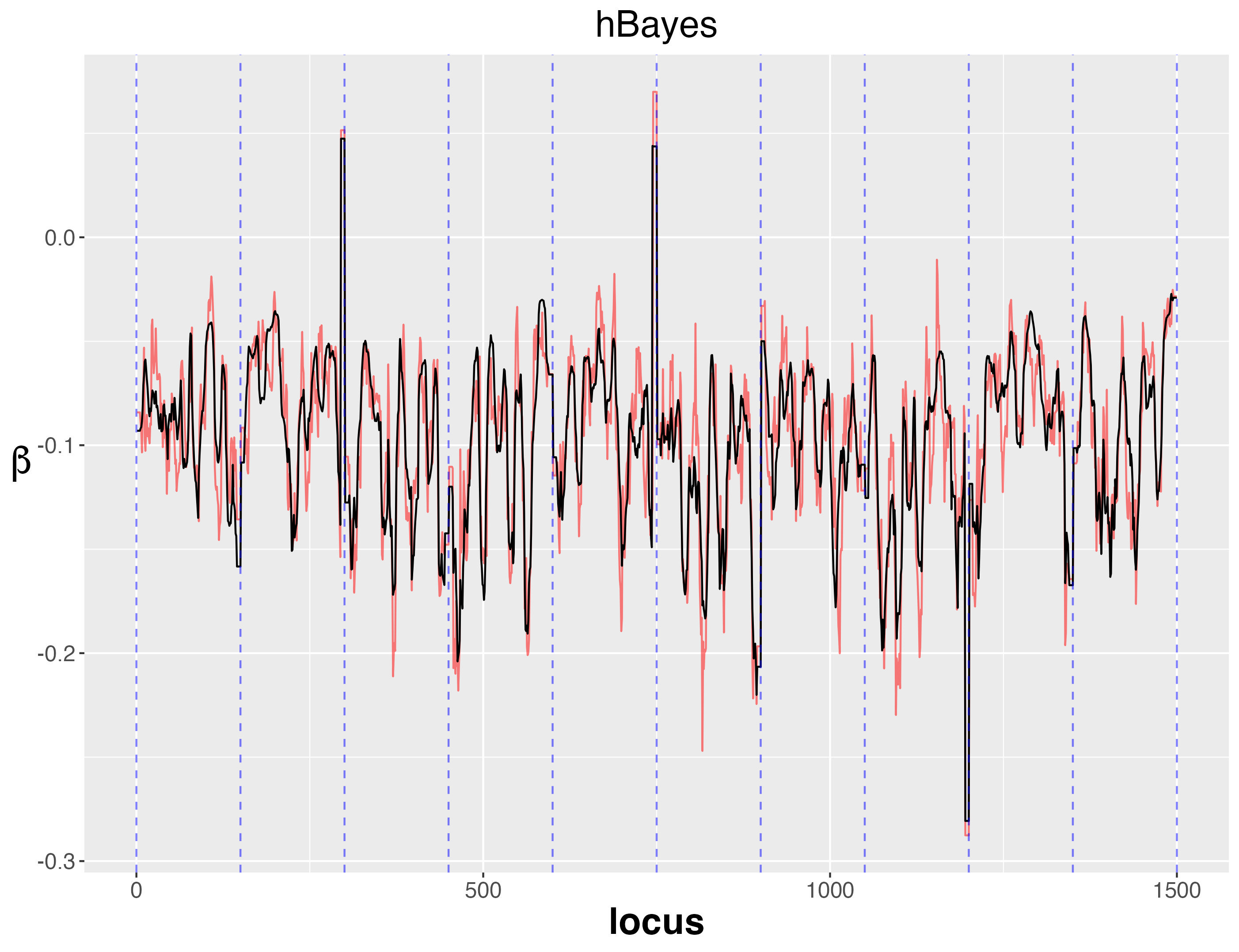
Figure 4: Results of the analysis of the simulated data. Going left to right, up to down we have: first plot is lasso, second is ridge, third is the Wallin et al. (2021) method based on the mixed effect model, fourth is our non-parametric Bayes approach. Red lines mark the true genetic effects and the black lines their estimates.

	lasso	ridge	mix	hBayes
MRSN of ${\bf X}\beta$	0.07	0.02	0.02	0.02
MRSN of $\beta$	0.89	0.96	0.77	0.76
MRSN of $\beta$ smooth	0.75	0.76	0.48	0.46

Table 2: The average relative root mean square error for 200 repeated simulations.

	${\bf\beta}_{1}$	${\bf\beta}_{2}$	${\bf\beta}_{3}$
lasso	0.11	0.11	0.09
ridge	0.19	0.19	0.18
mix	0.03	0.06	0.03
hBayes	0.05	0.07	0.04

Table 3: The average relative root mean square error for 200 repeated simulations.

smoothed	${\bf\beta}_{1}$	${\bf\beta}_{2}$	${\bf\beta}_{3}$
lasso	0.07	0.07	0.05
ridge	0.10	0.10	0.12
mix	0.02	0.02	0.02
hBayes	0.02	0.02	0.02

Table 4: The average relative root mean square error for 100 repeated simulations.

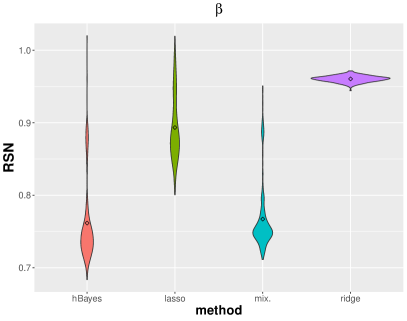
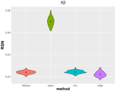
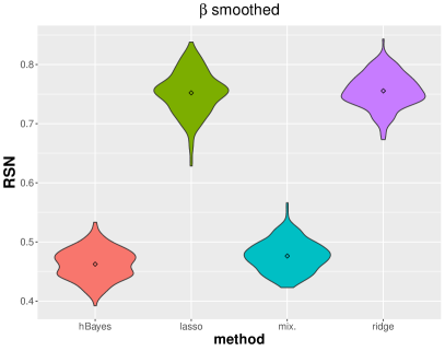
Figure 5: Distribution of RSN for the repeated simulations.

Figure 6: The estimated CDF for the hBayes (black curve) with pointwise 95% credibility intervals (dashed curve) from a sample versus the true cdf that generated the coefficients (red curve), i.e. the cdf of $\gamma+diag(e_{300}+e_{750}+e_{1200})\tilde{\beta}$.

5.2 Real Data Analysis

In this section we use our nonparametric Bayes approach to analyze the well known Zeng et al. (2000) Drosophila data. The purpose of the analysis is the identification of genes influencing the shape of the posterior lobe of the male genital arch in Drosophila. The size and shape variation of the males’ posterior lobes (which are highly correlated) are quantified by averaging over both sides of the morphometric descriptor (PC1) based on elliptical Fourier and principal components analyses.

The above mentioned data were extensively analyzed in Zeng et al. (2000), Bogdan et al. (2008) and Wallin et al. (2021), using different approaches based on the different multiple regression models. Zeng et al. (2000) and Bogdan et al. (2008) use the regular fixed effects multiple regression. Zeng et al. (2000) report 17 QTL, approximately uniformly distributed over the two chromosomes, with two of the strongest QTL located close to the centers of these chromosomes. The analysis in Bogdan et al. (2008) suggests that the likelihoods of several different multiple regression models are comparable and the positions of identified QTL differ substantially, depending on the number of assumed effects. In Wallin et al. (2021) the mixed effects multiple regression model was used, which allows for the presence of the polygenic effects, distributed all over the genome. The polygenic effects are modeled as i.i.d. random variables from a $\mathcal{N}(\mu,\tau^{2})$ distribution. According to the analysis reported in Wallin et al. (2021), the heritability of the considered trait reaches 72% and is attributed entirely to the polygenic effects.

In this Section we use our nonparametric Bayes approach to analyze the data from Zeng et al. (2000). The dataset includes genotypes of 39 markers on 2 autosomes for $n=491$ individuals. Following Bogdan et al. (2008)and Wallin et al. (2021), we used $m=161$ pseudo-marker explanatory variables spaced every 2 cM. The values of these pseudo-markers are calculated as the conditional expectations of the corresponding genotypes, given the genotypes of observed flanking markers, as in the regression interval mapping of Haley and Knott (1992). Such pseudo-marker explanatory variables are more strongly correlated than the markers spaced every 2cM. Thus, to curb the variance of locus specific estimates of regression coefficients, we performed our analysis using only every third of the pseudo-markers, i.e. using pseudo-markers spaced every 6cM.

Figure 7 provides 95% and 50% Bayesian credible intervals for the loci-specific genetic effects for our nonparametric approach, and the corresponding credibility intervals based on the random effects model considered in Wallin et al. (2021).

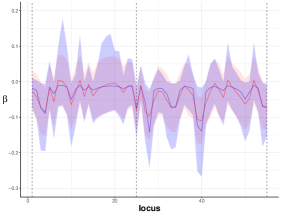
Figure 7: Posterior estimates of $\beta$ ordered on the chromosomes. The blue area corresponds to the pointwise credibility intervals for the nonparametric Bayes approach. The red area gives the confidence intervals for the random effect model of Wallin et al. (2021). The lines are the corresponding posterior means. The plot to the left presents the intervals for the coverage $5\%-95\%$, and to the right for the coverage $25\%-75\%$.

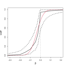
Figure 8: The cumulative distribution of $\beta$ for the random effects model of Wallin et al. (2021) (red line) and the median of its posterior distribution from the nonparametric Bayes approach (black line). The dashed lines are the pointwise $95\%$ credibility intervals.

Our analysis indicates a systematic negative polygenic effect, i.e. many relatively weak QTL effects of the negative sign on both chromosomes. The nonparametric Bayes estimates are more “peaky” than the estimates from a random effects model, especially in the direction of negative values. This difference is most visible in the plot of the 50% credible intervals, which in the case of the nonparametric Bayes approach are entirely contained on the side of negative values. Also, the median posterior distribution from the nonparametric Bayes approach is strongly asymmetric: it is almost truncated at zero, and has a relatively heavy negative tail. Heavy tails of the true polygenic distribution are also reflected in the 95% credible intervals, which are wider for the nonparametric Bayes approach than for the mixed model of Wallin et al. (2021). The normal random effects model seems to over-smooth, and also places more weight on the positive values. Despite these differences, the overall results from both methods are quite similar. Both methods yield the heritability (percentage of trait variability explained by genetic causes, $h^{2}=(\hat{\mathbb{V}}\left[Y\right]-\mathbb{E}\left[\sigma^{2}|{Y}\right])\big{/}\hat{\mathbb{V}}\left[Y\right]$) of $72\%$, and the 95% credible intervals for the posterior CDF of the polygenic effects cover the estimated normal prior for the random effects model. The main advantage of the proposed nonparametric Bayes approach is a more refined estimation for locations with increased strength of polygenic effects, and the capability of estimating a strongly asymmetric and heavy-tailed distribution of these effects.

6 Discussion

In this paper we have proposed a new nonparametric hierarchical Bayes estimator for high-dimensional GLMs. The method is inspired by an oracle shrinkage rule, defined as Bayes against the prior that assigns equal mass to every permutation of the true vector $\bm{\beta}$, and thus depending on $\bm{\beta}$ only through the empirical distribution of the components $\beta_{j}$. To justify this oracle as a benchmark, we show that it indeed has some optimality properties among all procedures which treat the components $\beta_{j}$ exchangeably. Importantly, our oracle rule is a well-defined object also in the frequentist setting, i.e., when the coefficient vector is truly fixed.

Our simulations demonstrate that, if the dimension of the problem is large, the proposed approach is able to approximate the oracle procedure, by implicitly learning the empirical distribution of the components of $\bm{\beta}$. Specifically, our numerical experiments demonstrate that our estimator is able to adapt nonparametrically to the correct shrinkage pattern in different settings, including sparse and dense configurations of the coefficient vector. The real data genetic example shows how our approach can be used to estimate the distribution of polygenic effects, which, in the real data example, turns out to be highly asymmetric and heavy-tailed. Normal random-effects models, typically used in this setup, are unable to identify this.

Challenges of different kinds certainly remain. From a theoretical viewpoint, it would be interesting to carry out a frequentist analysis of the estimator produced by the proposed hierarchical Bayes model. More specifically, we would like to investigate whether consistency results of the type proved in Castillo (2017) for density estimation with Polya tree priors, could be extended to the current situation where direct samples from the target density ($\beta_{j}$) are unobservable, but only noisy samples thereof ($y_{i}$).

On the methodological side, we plan to implement our modeling approach for studying polygenic effects in SNP or eQTL studies. First of all, note that the Gibbs sampling algorithms we apply that generate posterior samples of each model coefficient become computationally unviable for GLM with very large numbers of explanatory variables. While the oracle Bayes rule $\delta^{*}(\bm{y};\bar{\bm{\beta}})$ still retains its Bayesian optimality property, the explanatory variables in genomic models typically exhibit strong local dependencies that prohibits risk invariance with respect to the set of all permutations of the model coefficients, needed for ensuring that the oracle Bayes rule minimizes the risk for any value of $\bm{\beta}$. We propose to overcome both problems by adding another level in the hierarchy of the generative model for the data, representing the genetic effects within each genomic region, and use the components of $\bm{\beta}$ to specify the sum-effect allotted to the genomic regions. Hence, to derive the oracle Bayes rule, the Gibbs sampler will only need to generate posterior samples for the sum-effect of each genomic region, and the weak dependence between different genomic region will yield a model that is risk invariant with respect to permutations of $\bm{\beta}$.

Appendix A Sampling $\beta$

To sample the vector ${\bm{\mathrm{\beta}}}=\left(\beta_{1}\ldots\beta_{p}\right)$ given $(\psi,{\bm{\mathrm{\phi}}},\bm{y})$, we utilize a MH-within-Gibbs algorithm inspired by the coordinate descent algorithm of Friedman et al. (2007), that was shown to work very well for Lasso . Let $\bm{r}=(r_{1}\cdots r_{p})$ denote the index of the FPT subintervals to which each component of ${\bm{\mathrm{\beta}}}$ belongs, i.e. $r_{j}=k$ if $\beta_{j}\in{\cal I}_{L,k}$. We now detail how to generate a proposal for the MH algorithm for $\beta_{j}$:

1. Draw $r^{*}\sim r_{j}+Unif\{-K,\ldots,K\}$, where $K$ is a parameter which we estimate using an adaptive MCMC (AMCMC) scheme similar to Roberts and Rosenthal (2009). Specifically, we take an increasing batch size of MCMC samples; if the acceptance rate for the MH algorithm is above $0.3$ we increase $K$, if it is below $0.3$ we decrease it. The batch size is chosen such that updating is more seldom, in order to ensure convergence of the AMCMC algorithm.

2. Obtain a Taylor approximation of the log-likelihood $l(\beta_{j})=\log f\left(\bm{y}|{\bm{\mathrm{X}}},{\bm{\mathrm{\beta}}},\psi\right)$,

   $$l(\beta^{*}_{j})\approx l(\beta_{j})+l^{\prime}(\beta_{j})\left(\beta^{*}_{j}-\beta_{j}\right)+\frac{l^{\prime\prime}(\beta_{j})}{2}\left((\beta^{*}_{j}-\beta_{j}\right)^{2},$$

   where

   $$l^{\prime}(\beta_{j})=\frac{\partial}{\partial\beta_{j}}\log f\left(\bm{y}|{\bm{\mathrm{\beta}}},\psi\right)\ \ \ \ \ \text{and}\ \ \ \ \ l^{\prime\prime}(\beta_{j})=\frac{\partial^{2}}{\partial\beta^{2}_{j}}\log f\left(\bm{y}|{\bm{\mathrm{\beta}}},\psi\right).$$

3. Use the Taylor approximation to obtain a Normal approximation of the posterior as a proposal distribution, then generate a sample from the proposal given that proposal is contained in ${\cal I}_{L,r^{*}}$. That is, $\beta^{*}_{j}\sim\mathcal{N}_{{\cal I}_{L,r^{*}}}\left(\mu,\sigma^{2}\right)=\mathcal{N}\left(\mu,\sigma^{2}\right)|\{\beta^{*}_{j}\in{\cal I}_{L,r^{*}}\}$, where ${\cal I}_{L,r^{*}}=(a_{r^{*}},a_{r^{*}+1}]$, $\mu=\beta_{j}+\frac{l^{\prime}(\beta_{j})}{-l^{\prime\prime}(\beta_{j})}$, and $\sigma^{2}=\frac{1}{-l^{\prime\prime}(\beta_{j})}$.

Thus, we first generate an interval ${\cal I}_{L,r^{*}}$ that includes $\beta^{*}_{j}$, then, given that the prior is constant on the interval, we use a quadratic approximation of the likelihood to sample $\beta^{*}$ given it is in ${\cal I}_{L,r^{*}}$. Exactly as with coordinate descent algorithms, the main advantage of the algorithm is computational efficiency, for instance, one does not need to compute $\bm{X}\bm{\beta}$ in each iteration, but instead store $\hat{\bm{y}}=\bm{X}\bm{\beta}$ and then compute $\hat{\bm{y}}^{*}=\hat{\bm{y}}+\bm{x}^{T}_{j}\left(\beta^{*}_{j}-\beta_{j}\right)$. Hence, instead of computing a matrix-vector multiplication we only carry out a vector-scalar multiplication, and vector-addition. For the general likelihood (1), note that the log-likelihood, the gradient and the Hessian can be computed using only $\bm{X}\bm{\beta}$, and $\bm{x}_{j}$.

A.1 Sampling with oracle prior

Here we describe how to sample using MCMC when when the prior is the oracle prior $\pi_{0}$ defined in (11). Since the vector of unique coefficients are fixed we simple permute the locations randomly. To generate proposal ${\bm{\mathrm{\beta}}}^{*}$ given a previous sample ${\bm{\mathrm{\beta}}}$ we do as follows: first set ${\bm{\mathrm{\beta}}}^{*}={\bm{\mathrm{\beta}}}$, second generate two indices uniformly $i_{1},i_{2}\sim\mathcal{U}\{1,2,\ldots,p\}$ and set $\left(\beta^{*}_{i_{1}},\beta^{*}_{i_{2}}\right)=\left(\beta_{i_{2}},\beta_{i_{1}}\right)$. Clearly this proposal is symmetric, and since oracle prior is constant over the permutation, the Metropolis Hastings ratio is just $\frac{f({\bm{\mathrm{y}}}|{\bm{\mathrm{X}}},{\bm{\mathrm{\beta}}}^{*},\psi)}{f({\bm{\mathrm{y}}}|{\bm{\mathrm{X}}},{\bm{\mathrm{\beta}}},\psi)}$.

References

- Antoniak (1974) C. E. Antoniak. Mixtures of dirichlet processes with applications to bayesian nonparametric problems. The annals of statistics, pages 1152–1174, 1974.
- Bogdan et al. (2008) M. Bogdan, F. Frommlet, P. Biecek, R. Cheng, J. K. Ghosh, and R. W. Doerge. Extending the modified bayesian information criterion (mbic) to dense markers and multiple interval mapping. Biometrics, 64(4):1162–1169, 2008.
- Bogdan et al. (2013) M. Bogdan, E. van den Berg, W. J. Su, and E. J. Candès. Statistical estimation and testing via the sorted norm. arXiv preprint arXiv:1310.1969, 2013.
- Bogdan et al. (2015) M. Bogdan, E. van den Berg, C. Sabatti, W. J. Su, and E. J. Candès. Adaptive variable selection via convex optimization. Annals of Applied Statistics, 9(3):1103–1140, 2015.
- Brown et al. (2018) L. D. Brown, G. Mukherjee, and A. Weinstein. Empirical bayes estimates for a two-way cross-classified model. The Annals of Statistics, 46(4):1693–1720, 2018.
- Castillo (2017) I. Castillo. Pólya tree posterior distributions on densities. In Annales de l’Institut Henri Poincaré, Probabilités et Statistiques, volume 53, pages 2074–2102. Institut Henri Poincaré, 2017.
- Diaconis and Freedman (1980) P. Diaconis and D. Freedman. Finite exchangeable sequences. The Annals of Probability, pages 745–764, 1980.
- Efron and Morris (1975) B. Efron and C. Morris. Data analysis using stein’s estimator and its generalizations. Journal of the American Statistical Association, 70(350):311–319, 1975.
- Endelman (2011) J. B. Endelman. Ridge regression and other kernels for genomic selection with r package rrblup. The Plant Genome, 4:250–255, 2011.
- Ferguson (1973) T. S. Ferguson. A bayesian analysis of some nonparametric problems. The annals of statistics, pages 209–230, 1973.
- Ferguson (1974) T. S. Ferguson. Prior distributions on spaces of probability measures. The annals of statistics, 2(4):615–629, 1974.
- Fraser et al. (2010) H. B. Fraser, A. Moses, and E. E. Schadt. Evidence for widespread adaptive evolution of gene expression in budding yeast. Proceedings of the National Academy of Sciences of the United States of America, 107:2977–2982, 2010.
- Fraser et al. (2011) H. B. Fraser, T. Babak, J. Tsang, Y. Zhou, B. Zhang, M. Mehrabian, and E. E. Schadt. Systematic detection of polygenic cis-regulatory evolution. PLOS Genetics, 7(3):e1002023, 2011.
- Friedman et al. (2007) J. Friedman, T. Hastie, H. Höfling, and R. Tibshirani. Pathwise coordinate optimization. The Annals of Applied Statistics, 1(2):302 – 332, 2007. doi: 10.1214/07-AOAS131. URL https://doi.org/10.1214/07-AOAS131.
- Friedman et al. (2010) J. Friedman, T. Hastie, and R. Tibshirani. Regularization paths for generalized linear models via coordinate descent. Journal of Statistical Software, 33(1):1–22, 2010. doi: 10.18637/jss.v033.i01. URL https://www.jstatsoft.org/v33/i01/.
- George and Foster (2000) E. George and D. P. Foster. Calibration and empirical bayes variable selection. Biometrika, 87(4):731–747, 2000.
- Giri (1996) N. C. Giri. Group invariance in statistical inference. World Scientific, 1996.
- Greenshtein and Ritov (2009) E. Greenshtein and Y. Ritov. Asymptotic efficiency of simple decisions for the compound decision problem. Lecture Notes-Monograph Series, pages 266–275, 2009.
- Haley and Knott (1992) C. Haley and S. Knott. A simple regression method for mapping quantitative trait loci in line crosses using flanking markers. Heredity, 69:315–324, 1992.
- Hannan and Robbins (1955) J. F. Hannan and H. Robbins. Asymptotic solutions of the compound decision problem for two completely specified distributions. The Annals of Mathematical Statistics, pages 37–51, 1955.
- Hanson (2006) T. E. Hanson. Inference for mixtures of finite polya tree models. Journal of the American Statistical Association, 101(476):1548–1565, 2006.
- Hewitt and Savage (1955) E. Hewitt and L. J. Savage. Symmetric measures on cartesian products. Transactions of the American Mathematical Society, 80(2):470–501, 1955.
- James and Stein (1961) W. James and C. Stein. Estimation with quadratic loss. In Proceedings of the fourth Berkeley symposium on mathematical statistics and probability, volume 1, pages 361–379, 1961.
- Jiang et al. (2022) W. Jiang, M. Bogdan, J. Josse, B. Miasojedow, V. Rockova, and T. Group. Adaptive bayesian slope – high-dimensional model selection with missing values. Journal of Computational and Graphical Statistics, 31(1):113–137, 2022.
- Johnstone and Silverman (2004) I. M. Johnstone and B. W. Silverman. Needles and straw in haystacks: Empirical bayes estimates of possibly sparse sequences. The Annals of Statistics, 32(4):1594–1649, 2004.
- Kang et al. (2010) H. M. Kang, J. H. Sul, S. K. Service, N. A. Zaitlen, S. Y. Kong, N. B. Freimer, C. Sabatti, and E. Eskin. Variance component model to account for sample structure in genome- wide association studies. Nature Genetics, 42:348–354, 2010.
- Kim et al. (2022) Y. Kim, W. Wang, P. Carbonetto, and M. Stephens. A flexible empirical bayes approach to multiple linear regression and connections with penalized regression. arXiv preprint arXiv:2208.10910, 2022.
- Kou and Yang (2017) S. Kou and J. J. Yang. Optimal shrinkage estimation in heteroscedastic hierarchical linear models. In Big and Complex Data Analysis, pages 249–284. Springer, 2017.
- Lavine (1994) M. Lavine. More aspects of polya tree distributions for statistical modelling. The Annals of Statistics, 22(3):1161–1176, 1994.
- Leonard (1975) T. Leonard. Bayesian estimation methods for two-way contingency tables. Journal of the Royal Statistical Society: Series B (Methodological), 37(1):23–37, 1975.
- Lindley and Smith (1972) D. V. Lindley and A. F. Smith. Bayes estimates for the linear model. Journal of the Royal Statistical Society: Series B (Methodological), 34(1):1–18, 1972.
- Maldonado (2009) Y. M. Maldonado. Mixed models, posterior means and penalized least-squares. Optimality, 57:216–236, 2009.
- Oman (1982) S. D. Oman. Shrinking towards subspaces in multiple linear regression. Technometrics, 24(4):307–311, 1982.
- Piepho (2009) H.-P. Piepho. Ridge regression and extensions for genomewide selection in maize. Crop Science, 49:1165–1176, 2009.
- Price et al. (2008) A. L. Price, N. J. Patterson, D. Hancks, S. Myers, D. Reich, V. G. Cheung, and R. S. Spielman. Effects of cis and trans genetic ancestry on gene expression in african americans. PLOS Genetics, 4(12):e1000294, 2008.
- Robbins (1951) H. Robbins. Asymptotically subminimax solutions of compound statistical decision problems. In Proceedings of the second Berkeley symposium on mathematical statistics and probability, pages 131–149. University of California Press, 1951.
- Roberts and Rosenthal (2009) G. O. Roberts and J. S. Rosenthal. Examples of adaptive mcmc. Journal of Computational and Graphical Statistics, 18(2):349–367, 2009. doi: 10.1198/jcgs.2009.06134. URL https://doi.org/10.1198/jcgs.2009.06134.
- Ročková and George (2018) V. Ročková and E. I. George. The spike-and-slab lasso. Journal of the American Statistical Association, 113(521):431–444, 2018.
- Rolph (1976) J. E. Rolph. Choosing shrinkage estimators for regression problems. Communications in Statistics-Theory and Methods, 5(9):789–802, 1976.
- Ruppert et al. (2003) D. Ruppert, M. Wand, and R. Carroll. Semiparametric regression. Cambridge University Press, 2003.
- Sclove (1968) S. L. Sclove. Improved estimators for coefficients in linear regression. Journal of the American Statistical Association, 63(322):596–606, 1968.
- Stein (1956) C. Stein. Inadmissibility of the usual estimator for the mean of a multivariate normal distribution. In Proceedings of the Third Berkeley symposium on mathematical statistics and probability, volume 1, pages 197–206, 1956.
- Sur and Candès (2019) P. Sur and E. J. Candès. A modern maximum-likelihood theory for high-dimensional logistic regression. Proceedings of the National Academy of Sciences, 116(29):14516–14525, 2019.
- Turchin et al. (2012) M. Turchin, C. Chiang, C. Palmer, S. Sankararaman, D. Reich, C. GIANT, and J. N. Hirschhorn. Evidence of widespread selection on standing variation in europe at height-associated snps. Nature Genetics, 44:1015–1019, 2012.
- Vilhjálmsson and Nordborg (2013) B. Vilhjálmsson and M. Nordborg. The nature of confounding in genome-wide association studies. Nature Reviews Genetics, 14:1–2, 2013.
- Visscher and Haley (1996) P. M. Visscher and C. S. Haley. Detection of quantitative trait loci in line crosses under infinitesimal genetic models. Theoretical and Applied Genetics, 93:691–702, 1996.
- Wallin et al. (2021) J. Wallin, M. Bogdan, P. A. Szulc, R. W. Doerge, and D. O. Siegmund. Ghost QTL and hotspots in experimental crosses: novel approach for modeling polygenic effects. Genetics, 217(3), 01 2021. ISSN 1943-2631. doi: 10.1093/genetics/iyaa041. URL https://doi.org/10.1093/genetics/iyaa041. iyaa041.
- Weinstein (2021) A. Weinstein. On permutation invariant problems in large-scale inference. arXiv preprint arXiv:2110.06250, 2021.
- Yuan and Lin (2005) M. Yuan and Y. Lin. Efficient empirical bayes variable selection and estimation in linear models. Journal of the American Statistical Association, 100(472):1215–1225, 2005.
- Zeng et al. (2000) Z. Zeng, J. Liu, L. Stam, C. Kao, J. Mercer, and C. Laurie. Genetic architecture of a morphological shape difference between two drosophila species. Genetics, 154(1):299–310, 2000.
- Zhao et al. (2022) Q. Zhao, P. Sur, and E. J. Candes. The asymptotic distribution of the mle in high-dimensional logistic models: Arbitrary covariance. Bernoulli, 28(3):1835–1861, 2022.