CIMBA: fast Monte Carlo generation using cubic interpolation

Abstract

Monte Carlo generation of high energy particle collisions is a critical tool for both theoretical and experimental particle physics, connecting perturbative calculations to phenomenological models, and theory predictions to full detector simulation. The generation of minimum bias events can be particularly computationally expensive, where non-perturbative effects play an important role and specific processes and fiducial regions can no longer be well defined. In particular scenarios, particle guns can be used to quickly sample kinematics for single particles produced in minimum bias events. CIMBA (Cubic Interpolation for Minimum Bias Approximation) provides a comprehensive package to smoothly sample predefined kinematic grids, from any general purpose Monte Carlo generator, for all particles produced in minimum bias events. These grids are provided for a number of beam configurations including those of the Large Hadron Collider.

PROGRAM SUMMARY

Authors: Philip Ilten

Program Title: CIMBA (Cubic Interpolation for Minimum Bias Approximation)

Licensing provisions: GPL version 2 or later

Programming language: Python, C++

Computer: commodity PCs, Macs

Operating systems: Linux, OS X; should also work on other systems

RAM: $\sim$10 megabytes

Keywords: interpolation, Monte Carlo, event generators, phase space and event simulation

Classification: 11.2 Phase Space and Event Simulation

Nature of problem: generation of simulated events in high energy particle physics is quickly becoming a bottleneck in analysis development for collaborations on the Large Hadron Collider (LHC). With the expected long-term continuation of the high luminosity LHC, this problem must be solved in the near future. Significant progress has been made in designing new ways to perform detector simulation, including parametric detector models and machine learning techniques, e.g. calorimeter shower evolution with generative adversarial networks. Consequently, the efficiency of generating physics events using general purpose Monte Carlo event generators, rather than just detector simulation, needs to be improved.

Solution method: in many cases, single particle generation from pre-sampled phase-space distributions can be used as a fast alternative to full event generation. Phase-space distributions sampled in particle pseudorapidity and transverse momentum are sampled from large, once-off, minimum bias samples generated with Pythia 8. A novel smooth sampling of these distributions is performed using piecewise cubic Hermite interpolating polynomials. Distributions are created for all generated particles, as well as particles produced directly from hadronisation. Interpolation grid libraries are provided for a number of common collider configurations, and code is provided which can produce custom interpolation grid libraries.

Restrictions: single particle generation

Unusual features: none

Running time: $\mathcal{O}(10^{4})$ particles per second, depending on process studied

1 Introduction

Monte Carlo simulation of particle physics events provides a critical tool for calculating theory predictions, understanding detector performance, designing new detectors, developing experimental analysis techniques, and understanding experimental results [1]. Modern general purpose event generators [2, 3, 4] can simulate a broad range of physics processes, from minimum bias events to specific hard processes such as Higgs production. Final states from hard processes for a specific fiducial region corresponding to the acceptance for an experimental analysis can be selectively and efficiently simulated by choosing the relevant production channels and limiting the phase-space integration to the defined fiducial region. For the softer processes which constitute minimum bias events, such selectivity can no longer be applied at the perturbative level, as non-perturbative effects begin to have a much larger impact on the final state particles. Additionally, simulating minimum bias events can be computationally expensive; an average Large Hadron Collider (LHC) event can have hundreds of final state particles.

Consequently, simulating an exclusive final state from minimum bias events can require significant computing time. For example, $\approx 0.2$ $\phi$-mesons are produced on average per LHC minimum bias event, with no fiducial requirements. Applying a simple transverse requirement of ${p_{\mathrm{T}}}>1~{}\mathrm{GeV}$ and pseudorapidity requirement of $|\eta|<2.5$ reduces this even further to $\approx 0.05$. For more rare particles such as $B$-mesons or baryons, this suppression can be orders of magnitude larger, requiring millions of minimum bias events to be generated to produce a signal candidate. While this is typically not a problem for the ATLAS and CMS collaborations which focus on higher ${p_{\mathrm{T}}}$ physics, this is a significant issue for the LHCb collaboration, where most of the simulation is produced by extracting signal candidates from minimum bias simulation [5].

When only the signal candidate is needed, a particle gun technique can be used to more efficiently generate signal, where a probability density function (PDF) is used to quickly sample phase-space for the signal particle. Typically, this PDF is defined as a function of one or two variables, and is produced from a histogram, although other non-parametric estimation and simulation techniques could be used instead, see e.g. Reference [6] for an overview. The sharp edges of the histogram can produce artefacts in generated events. In Figure 1 a semi-realistic example is given, where the PDF for an arbitrary signal particle is given as a function of pseudorapidity. The actual closed form of this PDF is rarely known, but here a simplified double Gaussian distribution has been used. Assuming a fixed momentum of $10~{}\mathrm{GeV}$, the generated transverse momentum distribution is given, sampled from the actual PDF and the histogram PDF, resulting in a sharp edge at a transverse momentum of $\approx 4~{}\mathrm{GeV}$.

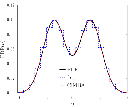
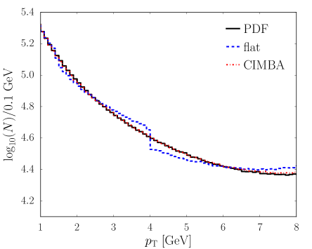
Figure 1: Simplified example of (left) a generating PDF and (right) a distribution generated from sampling the PDF.

The CIMBA package (Cubic Interpolation for Minimum Bias Approximation), available at gitlab.com/philten/cimba/, provides a complete framework for generating particles produced in minimum bias events, using a careful choice of generating PDF variables and smooth interpolation of the PDF. In the example of Figure 1, this smooth interpolation of the histogram PDF results in a nearly identical distribution to the true underlying distribution. The methods developed in this paper for sampling both univariate and bivariate interpolated distributions can also be applied outside the context of particle physics, where smooth sampling of discrete distributions is required. The remainder of this paper is organised as follows. In Section 2 the choice of univariate interpolation used for CIMBA is explained. In Section 3 the method for sampling this interpolation is derived and in Section 4 a method for sampling an interpolated bivariate PDF is introduced. The signal generation method for CIMBA is given in Section 5, while the structure of the CIMBA package is outlined in Section 6. Some examples, along with validation and performance, are explored in Section 7, and the paper is concluded in Section 8.

2 Univariate Interpolation

The piecewise interpolating polynomials, $f(x)$, for a PDF defined by a histogram, $h(x)$, with $n$ bin centres $x_{i}$ and bin values $y_{i}$ is given by,

$$f_{i}(x)=\sum_{l=0}^{k_{i}}{c_{i}^{(l)}}(x-x_{i})^{l},$$ (1)

given $x_{i}\leq x<x_{i+1}$, and $k_{i}$ is the degree of the interpolating polynomial $f_{i}$. For $f(x)$ to be both continuous and smooth, e.g. $C^{1}$, then $k\geq 3$. For most applications, $k=3$ is sufficient; in many cases using $k>3$ produces worse results due to Runge’s phenomenon [7].

For a histogram with $n\geq 3$, e.g. at least three bins, cubic interpolation can be performed with $n-1$ cubic functions $f_{i}$, resulting in $4(n-1)$ unknown coefficients ${c_{i}^{(l)}}$. A number of requirements, dependent on the interpolation method, must be placed on $f_{i}$ to determine ${c_{i}^{(l)}}$. In most methods, the piecewise interpolating function is required to be continuous,

$$f_{i}(x_{i})=h(x_{i})~{}\textrm{and}~{}f_{i}(x_{i+1})=h(x_{i+1}),$$ (2)

which specifies $2(n-1)$ constraints.

Cubic Hermite interpolation requires the first derivative at each point must also match,

$$\left.\frac{\mathrm{d}{f_{i}}}{\mathrm{d}{x}}\right|_{x_{i}}=\left.\frac{\mathrm{d}{h}}{\mathrm{d}{x}}\right|_{x_{i}}~{}\mathrm{and}~{}\left.\frac{\mathrm{d}{f_{i}}}{\mathrm{d}{x}}\right|_{x_{i+1}}=\left.\frac{\mathrm{d}{h}}{\mathrm{d}{x}}\right|_{x_{i+1}},$$ (3)

providing an additional $2(n-1)$ constraints. However, this requires the first derivative is known at each $x_{i}$. Monotone cubic Hermite interpolation (PCHIP) is the same as cubic Hermite interpolation, except the first derivative equality is relaxed when necessary to ensure the interpolating polynomial is monotonic over its interval of validity [8].

The unknown first derivative of $h(x)$ may be approximated as the average secant of the two neighbouring intervals for a given $x_{i}$,

$$\left.\frac{\mathrm{d}{h}}{\mathrm{d}{x}}\right|_{x_{i}}\approx\frac{1}{2}\left(\frac{y_{i}-y_{i-1}}{x_{i}-x_{i-1}}+\frac{y_{i+1}-y_{i}}{x_{i+1}-x_{i}}\right),$$ (4)

except for the endpoints $x_{1}$ and $x_{n}$. The derivative for these endpoints can be approximated using extrapolation. Assuming linear extrapolation, the first derivative is then defined as,

$$\left.\frac{\mathrm{d}{h}}{\mathrm{d}{x}}\right|_{x_{1}}\approx\frac{y_{2}-y_{1}}{x_{2}-x_{1}}~{}\mathrm{and}~{}\left.\frac{\mathrm{d}{h}}{\mathrm{d}{x}}\right|_{x_{n}}\approx\frac{y_{n}-y_{n-1}}{x_{n}-x_{n-1}},$$ (5)

for $x_{1}$ and $x_{n}$.

Natural cubic interpolation does not require knowledge of the first derivative of $h(x)$, but instead requires the first and second derivatives of the interpolating function are smooth,

$$\left.\frac{\mathrm{d}{f_{i}}}{\mathrm{d}{x}}\right|_{x_{i}}=\left.\frac{\mathrm{d}{f_{i}}}{\mathrm{d}{x}}\right|_{x_{i+1}}~{}\mathrm{and}\left.\frac{\mathrm{d}^{2}{f_{i}}}{\mathrm{d}{x}^{2}}\right|_{x_{i}}=\left.\frac{\mathrm{d}^{2}{f_{i}}}{\mathrm{d}{x}^{2}}\right|_{x_{i+1}},$$ (6)

e.g. $f(x)$ is $C^{2}$. This provides an additional $2(n-2)$ constraints. The final two constraints,

$$\left.\frac{\mathrm{d}^{2}{f_{1}}}{\mathrm{d}{x}^{2}}\right|_{x_{1}}=0~{}\mathrm{and}~{}\left.\frac{\mathrm{d}^{2}{f_{n-1}}}{\mathrm{d}{x}^{2}}\right|_{x_{n}}=0,$$ (7)

are required to fully specify the coefficients for $f_{i}$. Alternative constraints are the clamped boundary condition, where the first derivatives are required to be zero, and the not-a-knot boundary condition where the $x_{2}$ and $x_{n-1}$ third derivatives are required to be continuous.

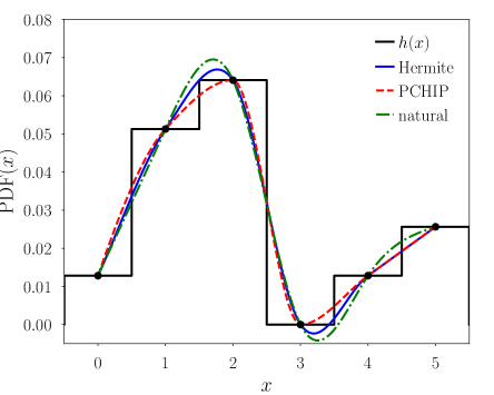
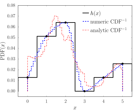
Figure 2: (left) Different methods of cubic interpolation and (right) demonstration of poor behaviour in the sampled PDF when interpolating the inverse CDF.

An example of Hermite, PCHIP, and natural cubic interpolation of a histogram $h(x)$ defining a PDF is given in Figure 2. While the normalisation of $h(x)$ is unity, this is not the case for the interpolating functions. Both the natural and Hermite interpolations fluctuate around the histogram bin centres, while the PCHIP interpolation does not. More importantly, because the PCHIP is monotonic and must pass through each bin centre, the resulting interpolation is guaranteed to always be positive. Neither the natural nor Hermite methods can guarantee a positive interpolation, making these two methods unsuitable for creating interpolated PDFs of histograms, and so the PCHIP method is used instead. Ideally, a modified PCHIP could be used, where the integral of the interpolating polynomial over each histogram bin yields the bin content.

3 Univariate Sampling

The PDF $g(x)$, defined over the interval $x_{\min}$ to $x_{\max}$, can be randomly sampled from a uniform distribution, $u\in[0,1]$, by taking $G^{-1}(u)$, where

$$G(x)=\int_{x_{\min}}^{x}\mathrm{d}{x^{\prime}}\,g(x^{\prime}),$$ (8)

is the cumulative distribution function (CDF) of $g(x)$ and $G^{-1}(u)$ is the inverse of this CDF. Naively, rather than analytically inverting $G(x)$ one could sample $G(x)$ at $x_{i}$, numerically invert the function by swapping $G(x_{i})$ with $x_{i}$, and interpolate the resulting points. However, if cubic interpolation of $G^{-1}(u)$ is used, the generated PDF is defined by second-order polynomials and typically has very poor behaviour, as shown in Figure 2. Consequently, analytic inversion of $G(x)$ is necessary.

The piecewise CDF of the interpolating functions $f_{i}(x)$ from Equation (1) is defined iteratively,

$$F_{i}(x)=F_{i-1}(x_{i})+\sum_{l=0}^{k_{i}}\frac{{c_{i}^{(l)}}}{l+1}(x-x_{i})^{l+1},$$ (9)

where ${c_{i}^{(l)}}$ are from the already normalised $f_{i}(x)$ and $F_{0}=0$. In practice, it is easier to use the coefficients from the unormalised $f(x)$ and sample $u\in[0,F_{n-1}(x_{n})]$ rather than over the unit interval.

To randomly sample this distribution $F_{i}^{-1}(u)$, the inverse of $F_{i}(x)$ must be taken, which requires solving up to a fourth-order polynomial,

$$0=F_{i-1}(x_{i})-u+\sum_{l=0}^{k_{i}}\frac{{c_{i}^{(l)}}}{l+1}(x-x_{i})^{l+1}$$ (10)

given $k=3$ and $F_{i}(x)=u$. For simplicity, the monic form of this polynomial is solved,

$$0=(x-x_{i})^{k_{i}}+\sum_{l=0}^{k_{i}}{m_{i}^{(l)}}(x-x_{i})^{l},$$ (11)

where $k_{i}$ is the highest non-zero order, ${m_{i}^{(0)}}=F_{i-1}(x_{i})-4u/{c_{i}^{(3)}}$, and ${m_{i}^{(l)}}=4{c_{i}^{(l-1)}}/(l{c_{i}^{(k)}})$ for $1\leq l\leq k$.

In the linear case there is a single solution to Equation (11)

$$F_{i}^{-1}(u)=-{m_{i}^{(0)}}/{m_{i}^{(1)}},$$ (12)

while for higher orders with multiple roots, the correct solution is the positive root closest to zero. For the quadratic case there are always two real roots and so,

$$F_{i}^{-1}(u)=\begin{cases}q&\text{if $q\geq 0$ and $q^{2}>{m_{i}^{(0)}}$}\\ {m_{i}^{(0)}}/q&\text{else,}\\ \end{cases}$$ (13)

where $q=-({m_{i}^{(1)}}+\mathrm{sgn}({m_{i}^{(1)}})\sqrt{{m_{i}^{(1)}}^{2}-4{m_{i}^{(0)}}^{2}})/2$. For the cubic case there can be either a single or three real roots,

$$F_{i}^{-1}(u)=\begin{cases}s+q/s-{m_{i}^{(2)}}/3&\text{if $p^{2}>q^{3}$}\\ 2\sqrt{q}\cos((\cos^{-1}(p/\sqrt{q^{3}})-2\pi)/3)-{m_{i}^{(2)}}/3&\text{else,}\\ \end{cases}$$ (14)

where $s=\mathrm{sgn}{(p)}(|p|+\sqrt{p^{2}-q^{3}})^{1/3}$, $p=(2{m_{i}^{(2)}}^{3}-9{m_{i}^{(2)}}{m_{i}^{(1)}}+27{m_{i}^{(0)}})/54$, and $q=({m_{i}^{(2)}}^{2}-3{m_{i}^{(1)}})/9$. Finally, for the quartic case,

$$F_{i}^{-1}(u)=-t(s-\sqrt{tq/s-p-4s^{2}}/2)-{m_{i}^{(3)}}/4,$$ (15)

given $p=(8{m_{i}^{(2)}}-3{m_{i}^{(3)}}^{2})/4$ and $q=({m_{i}^{(3)}}^{3}-4{m_{i}^{(3)}}{m_{i}^{(2)}}+8{m_{i}^{(1)}})/8$. When $d_{1}^{2}>4d_{0}^{3}$,

$$d_{0} ={m_{i}^{(2)}}^{2}-3{m_{i}^{(3)}}{m_{i}^{(1)}}+12{m_{i}^{(0)}}$$ (16)

$$d_{1} =2{m_{i}^{(2)}}^{3}-9{m_{i}^{(3)}}{m_{i}^{(2)}}{m_{i}^{(1)}}+27{m_{i}^{(3)}}^{2}{m_{i}^{(0)}}+27{m_{i}^{(1)}}^{2}-72{m_{i}^{(2)}}{m_{i}^{(0)}}$$

there are two real roots with the correct solution given by,

$$r =((d_{1}+\sqrt{d_{1}^{2}-4d_{0}^{3}})/2)^{1/3}$$ (17)

$$s =\sqrt{(r+d_{0}/r-p)/3}/2$$

$$t =\begin{cases}-1&\text{if $q/s-p-4s^{2}<0$}\\ 1&\text{else.}\\ \end{cases}$$

Otherwise, there are four real roots, with the correct solution given by,

$$s =((\sqrt{d_{0}}\cos(\cos^{-1}(d_{1}/(2d_{0}^{3/2}))/3)-p/2)/6)^{1/2}$$ (18)

$$t =\begin{cases}-1&\text{if ${m_{i}^{(3)}}/4+s>\sqrt{q/s-p-4s^{2}}/2$}\\ 1&\text{else.}\\ \end{cases}$$

The quadratic and cubic solutions are well conditioned numerically [9], while the quartic solution is not [10]. Currently, there is no numerically stable closed form for the quartic solution, although a generalised form of the cubic solvent is available, and could potentially be used to produce a numerically stable solution [11]. When the solution of Equation (15) fails numerically, a result will oftentimes be returned outside the interpolation interval and a more stable, albeit slower method, e.g. finding the eigenvalues of the companion matrix [12], can be used instead.

4 Bivariate Sampling

A bivariate PDF $g(x,y)$ can be sampled by factorising the generation into two univariate samplings. First project the PDF onto a single variable,

$$g(x)=\int_{y_{\min}}^{y_{\max}}\mathrm{d}{y}\,g(x,y)$$ (19)

and build the CDF for this projection, $G(x)$. A value for $x$ can then be generated using univariate sampling, e.g. from $G^{-1}(u)$. Given this $x$, a value for $y$ can be sampled with $G^{-1}(v|x)$ from a uniform distribution $v\in[0,1]$, where

$$G(y|x)=\int_{y_{\min}}^{y}\mathrm{d}{y^{\prime}}\,g(x,y^{\prime})$$ (20)

and $G^{-1}(v|x)$ is the inverse of $G(y|x)$. Again, this can be selected using univariate sampling.

Consider a bivariate PDF defined by a histogram $h(x,y)$ with $n$ $x$-bin centres of $x_{i,j}$, $m$ $y$-bin centres of $y_{i,j}$, and $n\times m$ bin contents $z_{i,j}$. Given PCHIP interpolation $f(x,y)$ of $h(x,y)$, the projected PDF $f(x)$ can be factored into arbitrary non-polynomial terms $\zeta_{i,j}$,

$$\sum_{j=1}^{m-2}\left(y_{i,j-1}-y_{i,j+1}\right)\left[(y_{i,j+1}-y_{i,j})-(y_{i,j+1}-y_{i,j-1})\right]\zeta_{i,j}(x),$$ (21)

and polynomial terms for each $f_{i}(x)$. The term in square brackets is the difference between two bin centres in $y$, so if the histogram has constant bin-spacing $\Delta y$, the $\zeta_{i,j}$ terms vanish, resulting in a third-degree polynomial to which the method of Section 3 can be applied.

Assuming constant $\Delta y$, the projected PDF is given by,

$$f_{i}(x)=\frac{\Delta y}{12}\sum_{l=0}^{k}x^{l}\begin{cases}5{c_{i,0}^{(l)}}+14{c_{i,1}^{(l)}}+5{c_{i,2}^{(l)}}&\text{if $m=3$,}\\ 5{c_{i,0}^{(l)}}+13{c_{i,1}^{(l)}}+13{c_{i,2}^{(l)}}+5{c_{i,3}^{(l)}}&\text{if $m=4$,}\\ 5{c_{i,0}^{(l)}}+13{c_{i,1}^{(l)}}+13{c_{i,m-2}^{(l)}}+5{c_{i,m-1}^{(l)}}+\sum_{j=2}^{m-3}12{c_{i,j}^{(l)}}&\text{else,}\\ \end{cases}$$ (22)

where $c_{i,j}^{(l)}$ are the coefficients for the interpolating function $f_{i}(x|j)$ for a given $y$-bin $j$. For example, $f_{i}(x|0)$ are the interpolating functions defined by the points $x_{i,0}$ and $z_{i,0}$ for the first $y$-bin with $j=0$. Consequently, coefficients for the $m$ interpolating functions $f_{i}(x|j)$ must be built to determine the coefficients for $f_{i}(x)$.

Using Equation (22) and the method of Section 3, an $x$-value can now be sampled. Given this $x$, the $f_{i}(x|j)$ can be used to calculate interpolated $z_{j}$ for each $y_{j}$. From these points the cubic interpolation function $f_{j}(y|x)$ can be sampled using the same process as for $x$. Note that to sample $y$ after an $x$ is given, $4m$ interpolation coefficients must be determined from $m$ interpolated values. This is computationally more expensive than just performing bicubic interpolation, which only requires $16$ interpolation coefficients from $4$ interpolated values.

5 Single Particle Generation

For the specific application of CIMBA, i.e. single particle generation from minimum bias events, each particle can be fully specified with a three-momentum, $(p_{x},p_{y},p_{z})$, and a mass, $m$. The mass of the particle is independent of its momentum, and can be sampled from a line-shape distribution given the nominal mass and width of the particle, leaving three unknowns. For colliders with unpolarised beams, particles are produced uniformly in azimuthal angle $\phi$ in the centre-of-mass (COM) frame, and so $\phi$ can also be sampled independently. This leaves two dependent variables which can be generated using the bivariate sampling of Section 4.

To minimise the effects of histogram binning, these two dependent variables should be chosen to have as flat of distributions as possible. In the COM frame, particle production is relatively constant in pseudorapidity, unlike the polar angle $\theta$, making this a natural choice. The remaining variable can then be either the magnitude of the momentum, $p$, or the transverse momentum, ${p_{\mathrm{T}}}$. At the LHC, particle production occurs primarily through $t$-channel processes, e.g. $gg\to q\bar{q}$ and $qq^{\prime}\to qq^{\prime}$, which are proportional to ${p_{\mathrm{T}}}^{-4}$. However, these processes are convolved with the proton PDF, modifying the ${p_{\mathrm{T}}}$ distribution.

The second variable is chosen as,

$${\rho}\equiv\frac{1}{({p_{\mathrm{T}}}+1~{}\mathrm{GeV}-{p_{\mathrm{T}}}_{\min})^{k}}$$ (23)

where ${p_{\mathrm{T}}}_{\min}$ is the minimum ${p_{\mathrm{T}}}$ requirement on produced particles, and $k$ is an arbitrary power. This variable is relatively flat, bounded between $0$ and $1$, the PDF must be $0$ at $\rho=0$, and can be reasonably calculated at $\rho=1$ via linear extrapolation. By default in CIMBA, ${p_{\mathrm{T}}}_{\min}=0.25~{}\mathrm{GeV}$ and $k=2$, although new grids can be generated by the user with different values. Here, $k=2$ is chosen as it provides a PDF that can smoothly interpolated to $0$ for $\rho=0$ and linearly extrapolated to $\rho=1$. The ${p_{\mathrm{T}}}_{\min}$ value is chosen for LHCb applications, where values below this cut-off are not experimentally accessible. In Figure 3 the projected PDF for $\rho$ with various $k$ and the bivariate PDF for $\rho$ and pseudorapidity is given for all final particles in LHC minimum bias events.

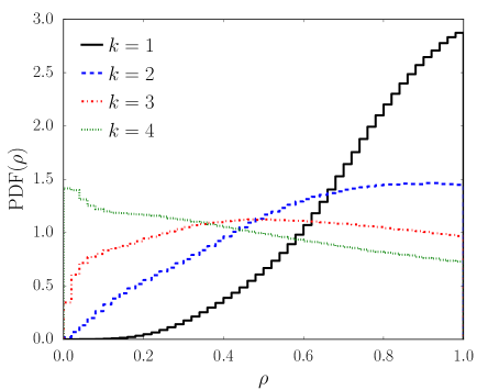
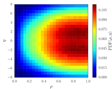
Figure 3: (left) PDF of $\rho$ for various $k$ and (right) bivariate PDF in $\rho$ (${p_{\mathrm{T}}}_{\min}=0.25~{}\mathrm{GeV}$ and $k=2$) and pseudorapidity, given for all final particles in LHC minimum bias events.

The default interpolation grids in pseudorapidity and $\rho$ are generated for the LHC using Pythia 8.240 [2] with the SoftQCD:all = on flag. Code is provided in CIMBA so that additional grids can be generated with Pythia for any COM energy and beam setup, e.g. proton-lead or proton-electron, and an arbitrary user configuration of Pythia. Regularisation of low ${p_{\mathrm{T}}}$ divergences for processes such as $gg\to b\bar{b}$ is performed using the same damping Pythia applies to soft QCD events. For some beam setups, like lepton-lepton, the selected physics processes need to modified as soft QCD production is no longer relevant. Additionally, user provided grids from other event generators can also be passed to CIMBA, assuming they are in the same format as the Pythia grids.

For each configuration, two sets of grids are provided.

• All particles produced in the event, including intermediate states. Only the final version of duplicate particles are included, e.g. for a gluon which undergoes multiple splittings, only the gluon from the final splitting is kept.

• Only particles produced directly from the hadronisation.

Because Pythia performs $B$-oscillations during the decay stage of the event generation, these are switched off to ensure double oscillations do not occur when passing generated $B$-mesons back to Pythia for subsequent decays.

6 Program Structure and Algorithms

The structure of the CIMBA package is summarised in Figure 4 where the class Histogram provides fast one dimensional bin finding using a modified regula falsi method; if regula falsi fails to find a bracketing interval, then the bisection method is used instead. The Histogram class acts as the base class for the PDF, CDF, and InverseCDF interpolation classes. The PDF class performs cubic interpolation using the PCHIP method outlined in Section 2, given an initial set of interpolating points. If provided with a set of PDF objects and corresponding $y$-values, the coefficients for the projected PDF of Equation (22) are built and used instead. The CDF class is initialised with a PDF object and returns the CDF defined by Equation (9). Note that the PDF does not need to be normalised, i.e. $F_{n-1}(x_{n})$ is not required to be unity, because the CDF class returns $F_{i}(x)/F_{n-1}(x_{n})$.

Figure 4: Structure of the CIMBA package with the dotted border boxes representing files and the solid border boxes representing classes. Solid arrows indicate inheritance, while dashed arrows indicate dependence. Colours indicate external module dependencies: grey is an optional numpy dependence, blue is a ROOT dependence, and red is a pythia8 dependence.

The InverseCDF class is also initialised with a PDF object, but returns the inverse CDF of the PDF as follows.

1. The $y$-values of the CDF are built by integrating the interpolating function over each interval from the PDF using Equation (9).

2. If limits are passed, e.g. the $x$-limits over which the inverse CDF is defined, the CDF values for these points are stored as $u_{0}$ and $u_{1}$ where $0\leq u_{0},u_{1}\leq 1$.

3. The $x$ and $y$-values are swapped.

4. When called with an argument $u$ between $0$ and $1$, the argument is transformed as $u^{\prime}=u_{0}+u(u_{1}-u_{0})$ to fall within the $x$-limits.

5. The modified regula falsi bin finding of the base Histogram class is used to determine interpolating interval $i$ for $u^{\prime}$.

6. Root finding using Equation (15) for interval $i$ is performed, given $u^{\prime}$, and the resulting $x$ is returned along with the weight $u_{1}-u_{0}$. If no $x$-limits have been required, this weight is unity.

7. If the analytic solution fails numerically, i.e. $x<x_{i}$ or $x>x_{i+1}$ the companion matrix method is used, as implemented in the roots method of the numpy package. If numpy is not available, linear interpolation is used.

The first three steps are only performed at initialisation of InverseCDF, while the remaining steps are performed each time an inverse CDF value is calculated.

The Sample1D class returns an $x$-value sampled from an interpolated PDF, given a uniform random number between $0$ and $1$. This is done by constructing an internal InverseCDF object and using this to calculate $x$ given $u$. Optionally, $x$-limits on the sampling range can be passed. The Sample2D class is similar to Sample1D but now returns a sampled $x$ and $y$-value with an associated weight using the method of Section 4 as follows.

1. A InverseCDF object is constructed for the projected PDF, given a PDF object for each $y$-value. The interpolating coefficients are calculated with Equation (22).

2. When passed two uniform random numbers, $u$ and $v$, an $x$-value and its corresponding weight $w_{x}$ is sampled from the projected InverseCDF.

3. Given this $x$, a PDF and subsequent InverseCDF, i.e. $G^{-1}(v|x)$, is built and a $y$-value with an associated weight $w_{y}$ is sampled.

4. The $x$ and $y$-values are returned with a weight of $w_{x}w_{y}$.

If no $y$-limit is placed on the sampling, the returned weight will be constant, and if additionally no $x$-limit is required, the returned weight will be unity. The first step is performed only during initialisation, while the remaining steps are performed for each sampling. The SampleTH1 and SampleTH2 classes provide convenient wrappers for sampling one and two-dimensional histograms from the ROOT package [13].

The PythiaDecay class takes three-momentum vectors sampled with the ParticleGun class and performs particle decays using the pythia8 module. The ParticleGun class uses the Sample2D class and the interpolation grids described in Section 5 to generate momentum three-vectors for a given particle type and set of sampling grids.

1. A PDF bivariate in $\rho$ and $\eta$ is built from the requested histogram and used to create an InverseCDF object.

2. Because the PDF at $\rho=0$ must be zero, i.e. particles are not produced with infinite transverse momentum, an additional point with a value of zero is inserted for each $\eta$ value with $\rho=0$.

3. Similarly, an additional point with a linearly extrapolated value is inserted for each $\eta$ value with $\rho=1$, if such a point does not already exist. This value is required to be $\geq 0$.

4. To generate a momentum three-vector, a value for $\rho$ and $\eta$ is sampled from the InverseCDF.

5. The transverse momentum is calculated as $\rho^{-1/k}-1~{}\mathrm{GeV}+{p_{\mathrm{T}}}_{\min}$.

6. The azimuthal angle $\phi$ is uniformly sampled between $0$ and $2\pi$, while $\cos(\theta)=(e^{2\eta}-1)(e^{2\eta}-1)$ and $\sin(\theta)=\sqrt{1-\cos^{2}(\theta)}$.

7. The three-momentum is returned as $[{p_{\mathrm{T}}}\cos(\phi),{p_{\mathrm{T}}}\sin(\phi),{p_{\mathrm{T}}}\cos(\theta)/\sin(\theta)]$ with a weight of $w_{\eta}$. The $\rho$-weight is included in the cross-section value.

The member sigma of the ParticleGun class provides the cross-section for the sampling in millibarn, given the ${p_{\mathrm{T}}}$-limits passed by the user, i.e. accounting for the $\rho$-weight. This is to ensure that sampling is not performed when the ${p_{\mathrm{T}}}$-limits produce a null interpolated phase-space. The same can not be done for the $\eta$-limits as the $\eta$-weight may be variable, given $\rho$. However, if the projected PDF in $\rho$ is non-zero, then for the sampled $\rho$ the $\eta$ PDF is guaranteed to have non-zero bins.

7 Validation, Performance, and Applications

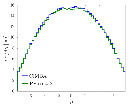
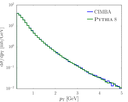
Figure 5: Comparison of CIMBA and Pythia generated (left) pseudorapidity and (right) transverse momentum distributions for $\pi^{+}$ production at the LHC.

The pseudorapidity and transverse momentum distributions of positively charged pions, $\pi^{+}$, produced by CIMBA and Pythia are compared in Figure 5. There is good agreement not only in the shape of the distributions, but also in the absolute normalisations, i.e. the predicted differential cross-sections. Tests have been performed for other particle species with similar levels of agreement observed. CIMBA can generate roughly 25 particles in the time that Pythia produces a single soft QCD event. In a typical LHC event, $\approx 30$ $\pi^{+}$ are produced on average with no fiducial requirements, and so for this worst case scenario, generation time for $30$ $\pi^{+}$ is roughly equivalent between CIMBA and Pythia. Realistic fiducial regions rapidly reduce the event multiplicity, e.g. requiring ${p_{\mathrm{T}}}>1~{}\mathrm{GeV}$ already reduces the $\pi^{+}$ multiplicity to $\approx 2$.

Six grid files, each generated from $10^{9}$ Pythia events, are provided with CIMBA.

• pp7TeV: soft QCD at the LHC with $\sqrt{s}=7~{}\mathrm{TeV}$.

• pp8TeV: soft QCD at the LHC with $\sqrt{s}=8~{}\mathrm{TeV}$.

• pp13TeV: soft QCD at the LHC with $\sqrt{s}=13~{}\mathrm{TeV}$.

• pp14TeV: soft QCD at the LHC with $\sqrt{s}=14~{}\mathrm{TeV}$.

• pp27GeV: soft QCD at SHiP with a proton beam energy of $400~{}\mathrm{GeV}$.

• ppbar980GeV: soft QCD at the Tevatron with $\sqrt{s}=980~{}\mathrm{GeV}$.

For each grid file, two sets of grids are provided: all which includes the final version of all particles produced in the event, and had where only particles produced directly from hadronisation are kept. From these grids, all single particle observables, for any particle species produced by Pythia, can be generated. Observables requiring particle correlations cannot be produced, e.g. jets. As detailed in Section 5, code is provided so new grids with different configurations may be generated by the user. Additionally, commonly used grids will be added to CIMBA upon request.

In the following examples, the estimated performance of CIMBA does not include the cost of generating the necessary interpolation grids. In principle, the entirety of the Pythia samples used to generate the CIMBA grids could be stored to disk. However, using naive storage techniques, this would require over $60~{}\mathrm{TB}$ of disk space per grid file. Simply accessing and storing such data would be computationally prohibitive. Reduced data could also be stored, i.e. four-vectors for a specific particle species, but then Pythia generation would be necessary whenever a new particle species was required. Finally, some particle species are produced so rarely by Pythia that smoothing would still be required when generating observables; CIMBA handles this transparently.

Two examples are given in Figure 6, demonstrating use cases for CIMBA. In the inclusive di-muon dark photon search proposal using LHCb Run 3 data of Reference [14], the dark-photon production rate is proportional to the expected electromagnetic (EM) background which is produced primarily from $\eta$, $\omega$, and $\rho$-meson decays, for dark photon masses less than $1~{}\mathrm{GeV}$. The results of CIMBA in Figure 6 agree well with the results of Reference [14]. Within the fiducial region of this search, on average $\approx 0.1$ $\eta$ mesons are produced per event and so using CIMBA corresponds to an $\approx 250\times$ speedup. A sample which would previously take on the order of a week to produce, can now be generated in roughly a half hour. This is particularly useful for determining expected experimental reach for new physics produced from light mesons. Similarly, when recasting dark photon results to non-minimal models [15] the ratio between production mechanisms is needed, which can now be quickly calculated with CIMBA.

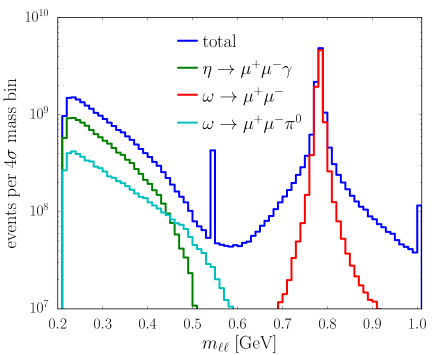
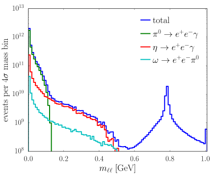
Figure 6: CIMBA generated (right) di-muon mass spectrum for LHCb Run 3 following the proposed dark photon search of Reference [14] and (left) di-electron mass spectrum following the proposed true muonium search of Reference [16].

The displaced background for the inclusive di-muon dark photon search of Reference [14] at low dark photon masses is primarily from semi-leptonic $B$-meson decays of the form $B\to\mu D[\to\mu X]$. Only $<0.01$ $B$-mesons per event are in the fiducial region of the search; generation with CIMBA results in a $>2500\times$ speedup. Of course, a more strategic generation of events could be performed with Pythia, e.g. generating HardQCD:hardbbbar events with minimum transverse momentum cuts. However, strategies such as this oftentimes result in the loss of some physics processes, in this case the production of $B$-mesons from gluon splitting in events without a hard $b\bar{b}$ process. In the LHCb dark photon search of Reference [17], an implementation of Reference [14], large generated samples of $B\to\mu D[\to\mu X]$ events were required to create a displaced background template. With CIMBA, higher statistics and more detailed generation of this background can be achieved.

The ${}^{3}S_{1}$ state of true muonium, a bound di-muon atom, can be produced in a similar fashion to dark photons, with the notable exception that true muonium has a small binding energy of $1.4~{}\mathrm{keV}$ and will typically dissociate upon impact with detector material. In Reference [16] a search proposal for true muonium using di-electron final states from $\eta$-meson decays in LHCb Run 3 data is outlined. In Figure 6 the di-electron mass distribution is given for this search proposal, as generated by CIMBA. Note that there is no $\eta\to ee$ peak, unlike the $\eta\to\mu\mu$ peak, as this decay channel is helicity suppressed by a factor of $m_{e}^{2}/m_{\mu}^{2}$. The result agrees well with the prediction of $\approx 3400$ TM events from Reference [16], given a signal to EM background ratio of $1.2\times 10^{-6}$ for a $4\sigma$ mass bin. Here, the full mass distribution is given, which can also be used to determine a naive reach for dark photon searches with di-electron final states.

Both the dark photon and true muonium examples are provided in the dilepton.py example in the CIMBA package. After particle generation with CIMBA, decays are performed using Pythia. All relevant di-lepton decays are determined using the Pythia decay tables. In this example CIMBA automatically estimates the branching fractions for missing di-lepton channels in Pythia by scaling the branching ratio for the equivalent channel with a photon by a factor of $\alpha$, neglecting phase-space suppression. For example, the decay $\eta\to\mu^{+}\mu^{-}\pi^{+}\pi^{-}$ is missing in Pythia, so its branching fraction is calculated from the channel $\eta\to\gamma\pi^{+}\pi^{-}$. In this particular case, the branching ratio is estimated to be $3.4\times 10^{-4}$ but the expected branching ratio is $1.2\times 10^{-8}$ [18] and so this channel is added explicitly.

No explicit attempt has been made at evaluating the uncertainty introduced via the interpolation methods of CIMBA. This is because CIMBA is intended for use within the non-perturbative QCD regime, where the tune of the event generator producing the interpolation grids is expected to be the primary source of systematic uncertainty. However, the uncertainty introduced via interpolation can be estimated by re-binning the interpolation grids, e.g. halve the number of bins, and calculating the difference in shapes between the fine and coarse interpolation grids.

8 Conclusions

Generating kinematics for single particles produced in simulated minimum bias events at the LHC within well defined fiducial regions can be computationally expensive, particularly for particle types rarely produced in the hadronisation process. This can be problematic for experiments such as LHCb, where the majority of simulation samples are extracted from generated minimum bias events. The CIMBA package provides a lightweight and fast particle gun method to generate smooth interpolated distributions of such particles with well defined fiducial regions in pseudorapidity and transverse momentum. The efficacy of CIMBA is demonstrated by reproducing the results from proposed dark photon and true muonium searches with LHCb. These results were generated on the order of minutes, rather than the previous computation time on the order of weeks. Additionally, this method for sampling distributions from cubic interpolated histograms, both univariate and bivariate, has applications outside of particle physics where smooth sampling is required from non-parametric distributions.

9 Acknowledgements

We thank Stephen Farry, Jonathan Plews, Yotam Soreq, and Nigel Watson for providing useful feedback and testing. PI is supported by a Birmingham Fellowship.

Bibliography

Bibliography

- [1] A. Buckley, et al., General-purpose event generators for LHC physics, Phys. Rept. 504 (2011) 145–233. arXiv:1101.2599, doi:10.1016/j.physrep.2011.03.005.
- [2] T. Sjöstrand, S. Ask, J. R. Christiansen, R. Corke, N. Desai, P. Ilten, S. Mrenna, S. Prestel, C. O. Rasmussen, P. Z. Skands, An Introduction to PYTHIA 8.2, Comput. Phys. Commun. 191 (2015) 159–177. arXiv:1410.3012, doi:10.1016/j.cpc.2015.01.024.
- [3] E. Bothmann, et al., Event Generation with SHERPA 2.2arXiv:1905.09127.
- [4] J. Bellm, et al., Herwig 7.0/Herwig++ 3.0 release note, Eur. Phys. J. C76 (4) (2016) 196. arXiv:1512.01178, doi:10.1140/epjc/s10052-016-4018-8.
- [5] I. Belyaev, et al., Handling of the generation of primary events in Gauss, the LHCb simulation framework, J. Phys. Conf. Ser. 331 (2011) 032047. doi:10.1088/1742-6596/331/3/032047.
- [6] J. R. Thompson, R. A. Tapia, Nonparametric function estimation, modeling, and simulation, Vol. 21, Siam, 1990.
- [7] C. Runge, Über empirische Funktionen und die Interpolation zwischen äquidistanten Ordinaten, Zeitschrift für Mathematik und Physik 46 (224-243) (1901) 20.
- [8] F. N. Fritsch, R. E. Carlson, Monotone piecewise cubic interpolation, SIAM Journal on Numerical Analysis 17 (2) (1980) 238–246.
-
[9]
W. H. Press, S. A. Teukolsky, W. T. Vetterling, B. P. Flannery,
Numerical recipes in C++: the art
of scientific computing; 2nd ed., Cambridge Univ. Press, Cambridge, 2002.
URL https://cds.cern.ch/record/542667 - [10] D. Herbison-Evans, Solving Quartics and Cubics for Graphics, Academic Press, Boston, 1995. doi:10.1016/B978-0-12-543457-7.50009-7.
- [11] S. Shmakov, A universal method of solving quartic equations, International Journal of Pure and Applied Mathematics 71 (2011) 251.
- [12] R. A. Horn, C. R. Johnson, Matrix Analysis, 2nd Edition, Cambridge University Press, New York, NY, USA, 2012.
- [13] R. Brun, F. Rademakers, ROOT: An object oriented data analysis framework, Nucl. Instrum. Meth. A389 (1997) 81–86. doi:10.1016/S0168-9002(97)00048-X.
- [14] P. Ilten, Y. Soreq, J. Thaler, M. Williams, W. Xue, Proposed Inclusive Dark Photon Search at LHCb, Phys. Rev. Lett. 116 (25) (2016) 251803. arXiv:1603.08926, doi:10.1103/PhysRevLett.116.251803.
- [15] P. Ilten, Y. Soreq, M. Williams, W. Xue, Serendipity in dark photon searches, JHEP 06 (2018) 004. arXiv:1801.04847, doi:10.1007/JHEP06(2018)004.
- [16] X. Cid Vidal, P. Ilten, J. Plews, B. Shuve, Y. Soreq, Discovering True Muonium at LHCbarXiv:1904.08458.
- [17] R. Aaij, et al., Search for Dark Photons Produced in 13 TeV Collisions, Phys. Rev. Lett. 120 (6) (2018) 061801. arXiv:1710.02867, doi:10.1103/PhysRevLett.120.061801.
- [18] A. Faessler, C. Fuchs, M. I. Krivoruchenko, Dilepton spectra from decays of light unflavored mesons, Phys. Rev. C61 (2000) 035206. arXiv:nucl-th/9904024, doi:10.1103/PhysRevC.61.035206.