Decentralized Cooperative Online Estimation With Random Observation Matrices, Communication Graphs and Time Delays

Abstract

We analyze convergence of decentralized cooperative online estimation algorithms by a network of multiple nodes via information exchanging in an uncertain environment. Each node has a linear observation of an unknown parameter with randomly time-varying observation matrices. The underlying communication network is modeled by a sequence of random digraphs and is subjected to nonuniform random time-varying delays in channels. Each node runs an online estimation algorithm consisting of a consensus term taking a weighted sum of its own estimate and neighbours’ delayed estimates, and an innovation term processing its own new measurement at each time step. By stochastic time-varying system, martingale convergence theories and the binomial expansion of random matrix products, we transform the convergence analysis of the algorithm into that of the mathematical expectation of random matrix products. Firstly, for the delay-free case, we show that the algorithm gains can be designed properly such that all nodes’ estimates converge to the true parameter in mean square and almost surely if the observation matrices and communication graphs satisfy the stochastic spatio-temporal persistence of excitation condition. Secondly, for the case with time delays, we introduce delay matrices to model the random time-varying communication delays between nodes. It is shown that under the stochastic spatio-temporal persistence of excitation condition, for any given bounded delays, proper algorithm gains can be designed to guarantee mean square convergence for the case with conditionally balanced digraphs.

I introduction

Estimation algorithms have important applications in many fields, e.g. navigation systems, space exploration, machine learning and power systems ([1]-[4]), etc. In a power system, measurement devices such as remote terminal units and phasor measurement units, send the measured active and reactive power flows, bus injection powers and voltage amplitudes to the Supervisory Control and Data Acquisition (SCDA) system, then the voltage amplitudes and phase angles at all buses are estimated for secure and stable operation of the system ([5]-[6]). Generally speaking, there are mainly two categories of estimation algorithms in term of information structure, i.e. centralized and decentralized algorithms. In a centralized algorithm, a fusion center is used to collect all nodes’s measurements and gives the global estimate. This structure heavily relies on the fusion center and lacks robustness and security. In a decentralized algorithm, a network of multiple nodes is employed to cooperatively estimate the unknown parameter via information exchanging, where each node is an entity with integrated capacity of sensing, computing and communication, and occasional node/link failures may not destroy the entire estimation task. Hence, decentralized cooperative estimation algorithms are more robust than centralized ones ([7]-[8]).

There exist various kinds of uncertainties in real networks. For example, sensors are usually powered by chemical or solar cells, and the unpredictability of cell power leads to random node/link failures, which can be modeled by a sequence of random communication graphs. Besides, node sensing failures or measurement losses ([9]) can be modeled by a sequence of random observation matrices. There are lots of literature on decentralized online estimation problems with random graphs. Ugrinovskii [10] studied decentralized estimation with Markovian switching graphs. Kar & Moura [11] and Sahu $et~{}al$ [12] considered decentralized estimation with i.i.d. graph sequences, where Kar & Moura [11] showed that the algorithm achieves weak consensus under a weak distributed detectability condition and Sahu $et~{}al$ [12] proved that the algorithm converges almost surely if the mean graph is balanced and strongly connected. Simões & Xavier [13] proposed a decentralized estimation algorithm with i.i.d. undirected graphs and proved that the convergence rate of mean square estimation error is asymptotically equal to that of the centralized algorithm. Decentralized cooperative online estimation based on diffusion strategies was addressed in [14]-[18] with spatio-temporally independent observation matrices, i.e. the sequence of observation matrices of each node is an independent random process and those of different nodes are mutually independent. Piggott & Solo [19]-[20] studied decentralized estimation with temporally correlated observation matrices and a fixed communication graph. Ishihara & Alghunaim [21] studied decentralized estimation with spatially independent observation matrices. Kar $et~{}al$ [22] and Kar & Moura [23] proposed consensus+innovations decentralized estimation algorithms with random graphs and observation matrices, where the sequences of communication graphs and observation matrices are both i.i.d. They proved that the algorithm converges almost surely if the mean graph is balanced and strongly connected. Zhang & Zhang [24] considered decentralized estimation with finite Markovian switching graphs and i.i.d. observation matrices, and proved that the algorithm converges in mean square and almost surely if all graphs are balanced and jointly contain a spanning tree. Zhang $et~{}al$ [25] proposed a robust decentralized estimation algorithm with the communication graphs and observation matrices being mutually independent with each other and both uncorrelated sequences. In summary, most existing literature on decentralized cooperative estimation algorithms required balanced mean graphs and special statistical properties of communication graphs and observation matrices, such as i.i.d. or Markovian switching graph sequences, spatially or temporally independent observation matrices with the fixed mathematical expectation, which are also independent of communication graphs.

Besides random communication graphs and observation matrices, random communication delays are also common in real systems ([26]-[28]). Due to congestions of communication links and external interferences, time delays are usually random and time-varying, whose probability distribution can be approximately estimated by statistical methods. However, to our best knowledge, there has been no literature on decentralized online estimation with general random time-varying communication delays. Zhang $et~{}al$ [29] and Millán $et~{}al$ [30] considered decentralized estimation with uniform deterministic time-invariant and time-varying communication delays, respectively, where Millán $et~{}al$ [30] established a LMI type convergence condition by the Lyapunov-Krasovskii functional method.

In this paper, we analyze convergence of decentralized cooperative online parameter estimation algorithms with random observation matrices, communication graphs and time delays. Each node’s algorithm consists of a consensus term taking a weighted sum of its own estimate and delayed estimates of its neighbouring nodes, and an innovation term processing its own new measurement at each time step. The sequences of observation matrices, communication graphs and time delays are not required to satisfy special statistical properties, such as mutual independence and spatio-temporal independence. Furthermore, neither the sample paths of the random graphs nor the mean graphs are necessarily balanced and connected at each time step. These relaxations together with the existence of random time-varying time delays bring essential difficulties to the convergence analysis, and most existing methods are not applicable. For example, the frequency domain approach ([29],[31]) is only suitable for deterministic uniform time-invariant time delays, and the Lyapunov-Krasovskii functional method leads to a non-explicit LMI type convergence condition ([30]). Liu $et~{}al$ [32] and Liu $et~{}al$ [33] addressed distributed consensus with deterministic time-varying communication delays and i.i.d. communication graphs. The analysis method therein required the mean graph to be time-invariant and connected at each time step, and is not applicable to time-varying mean graphs.

We introduce delay matrices to model the random time-varying communication delays between each pair of nodes. By stochastic time-varying system, martingale convergence theories and the binomial expansion of random matrix products, we transform the convergence analysis of the algorithm into that of the mathematical expectation of random matrix products. Firstly, for the delay-free case, we show that the algorithm gains can be designed properly such that all nodes’ estimates converge to the true parameter in mean square and almost surely if the observation matrices and communication graphs satisfy the stochastic spatio-temporal persistence of excitation conditions. Especially, it is shown that for Markovian switching communication graphs and observation matrices, this condition holds if the stationary graph is balanced with a spanning tree and the measurement model is spatio-temporally jointly observable. Secondly, for the case with time delays, we propose several conditions for mean square convergence, which explicitly relies on the conditional expectations of delay matrices, observation matrices and weighted adjacency matrices of communication graphs over a sequence of fixed-length time intervals. Furthermore, we show that if the communication graphs are conditionally balanced, then under the stochastic spatio-temporal persistence of excitation condition, for any given bounded delays, proper algorithm gains can be designed to guarantee mean square convergence of the algorithm. Compared with the existing literature, our contributions are summarized as below.

• The delay-free case

  • We show that it is not necessary that the sequences of observation matrices and communication graphs be mutually independent or spatio-temporally independent. Also, the mean graphs are not necessarily time-invariant and balanced. We establish the stochastic spatio-temporal persistence of excitation condition under which the algorithm with random graphs and observation matrices converges in mean square and almost surely. For a network consisting of completely isolated nodes, the stochastic spatio-temporal persistence of excitation condition degenerates to a set of independent stochastic persistence of excitation conditions for centralized algorithms ([38]).

  • Especially, for the case with Markovian switching communication graphs and observation matrices, we prove that the stochastic spatio-temporal persistence of excitation condition holds if the stationary graph is balanced with a spanning tree and the measurement model is spatio-temporally jointly observable, implying that neither local observability of each node nor instantaneous global observability of the entire measurement model is necessary.

• The case with time delays

  • We introduce delay matrices to model the random time-varying time delays between each pair of nodes. By the method of binomial expansion of random matrix products, we obtain several conditions for mean square convergence, which explicitly relies on the conditional expectations of the delay matrices, observation matrices and weighted adjacency matrices of communication graphs over a sequence of fixed-length time intervals. These conditions show that for given algorithm gains, the communication graphs and observation matrices need to be persistently excited with enough intensity to mitigate the random time delays. We further show that if the stochastic spatio-temporal persistence of excitation condition holds, then for any given bounded delays, proper algorithm gains can be designed to guarantee mean square convergence of the algorithm for the case with conditionally balanced digraphs.

  • The nonuniform random time-varying communication delays considered in this paper are more general, and we allow correlated communication delays, graphs and observation matrices.

The rest of the paper is arranged as follows. In Section II, we formulate the problem. In Section III, we describe the decentralized cooperative online parameter estimation algorithm with random observation matrices, communication graphs and time delays. We make the convergence analysis for the delay-free case and the case with time delays in Sections IV and V, respectively. In Section VI, we give a numerical example to demonstrate the theoretical results. Finally, we conclude the paper and give some future topics in Section VII.

Notation and symbols: $\circ$: the Hadamard product; $\otimes$: the Kronecker product; $\mathrm{Tr}(A)$: the trace of matrix $A$; $\|A\|$: the 2-norm of matrix $A$; $A^{T}$: the transpose of matrix $A$; $\mathbb{P}\{A\}$: the probability of event $A$; $I_{n}$: the $n$ dimensional identity matrix; $\rho(A)$: the spectral radius of matrix $A$; $|a|:$ the absolute value of real number $a$; $\mathbb{R}^{n}$: the $n$ dimensional real vector space; $A\geq B$: the matrix $A-B$ is positive semidefinite; $\lfloor x\rfloor$: the largest integer less than or equal to $x$; $\lceil x\rceil$: the smallest integer greater than or equal to $x$; $\mathbb{E}[\xi]$: the mathematical expectation of random variable $\xi$; $\lambda_{\min}(A)$: the minimum eigenvalue of real symmetric matrix $A$; $\textbf{1}_{n}$: the $n$ dimensional column vector with all entries being one; $\textbf{0}_{n\times m}$: the $n\times m$ dimensional matrix with all entries being zero; $b_{n}=O(r_{n})$: $\lim\sup_{n\to\infty}\frac{|b_{n}|}{r_{n}}<\infty$, where $\{b_{n},n\geq 0\}$ is a sequence of real numbers, $\{r_{n},n\geq 0\}$ is a sequence of real positive numbers;  $b_{n}=o(r_{n})$: $\lim_{n\to\infty}\frac{b_{n}}{r_{n}}=0$; For a sequence of $n\times n$ dimensional matrices $\{Z(k),k\geq 0\}$ and a sequence of scalars  $\{c(k),k\geq 0\}$, denote

$$\Phi_{Z}(j,i)=\left\{\begin{array}[]{cc}Z(j)\cdots Z(i),&~{}j\geq i\\ I_{n},&~{}j<i.\end{array}\right.\mathrm{and}~{}~{}\prod_{k=i}^{j}c(k)=\left\{\begin{array}[]{cc}c(j)\cdots c(i),&~{}j\geq i\\ 1,&~{}j<i.\end{array}\right.$$

For any nonnegative integers $i$ and $j$, denote the Kronecker function by $\mathcal{I}_{i,j}$, satisfying $\mathcal{I}_{i,j}=1$ if $i=j$ and $\mathcal{I}_{i,j}=0$ otherwise.

II problem formulation

II-A Measurement model

Consider a network of $N$ nodes. Each node is an estimator with integrated capacity of sensing, computing, storage and communication. The estimators/nodes cooperatively estimate an unknown parameter vector $x_{0}\in\mathbb{R}^{n}$ via information exchanging. The relation between the measurement vector $z_{i}(k)\in\mathbb{R}^{n_{i}}$ of estimator $i$ and the unknown parameter $x_{0}$ is represented by

$$z_{i}(k)=H_{i}(k)x_{0}+v_{i}(k),\ i=1,\cdots,N,\ k\geq 0.$$ (2)

Here, $H_{i}(k)\in\mathbb{R}^{n_{i}\times n}$ is the random observation (regression) matrix at time instant $k$ with $n_{i}\leq n$, and $v_{i}(k)\in\mathbb{R}^{n_{i}}$ is the additive measurement noise. Denote $z(k)=[z_{1}^{T}(k),\cdots,z_{N}^{T}(k)]^{T}$, $H(k)=[H_{1}^{T}(k),\cdots,H_{N}^{T}(k)]^{T}$ and $v(k)=[v_{1}^{T}(k),\cdots,v_{N}^{T}(k)]^{T}$. Rewrite (2) by the compact form

$$z(k)=H(k)x_{0}+v(k),\ k\geq 0.$$ (3)

Remark 1.

In many real applicaitons, the relations between the unknown parameter and the measurements can be represented by (2). For example, in the decentralized multi-area state estimation in power systems, the grid is partitioned into multiple geographically non-overlapping areas, and each area is regarded as a node. The grid state $x_{0}$ to be estimated consists of voltage amplitudes and phase angles at all buses. The measurement $z_{i}(k)$ of each area/node consists of the active and reactive power flow, bus injection powers and voltage amplitude information measured by remote terminal units and phasor measurement units in the $i$-th area. By the DC power flow approximation ([34]), the grid state degenerates to the voltage phase angles at all buses and the relation between the measurement of each area and the grid state can be represented by (2). In decentralized parameter identification, each node’s measurement equation is given by

$$z_{i}(k)=\sum_{j=1}^{n}c_{j}z_{i}(k-j)+v_{i}(k)=[z_{i}(k-1),\cdots,z_{i}(k-n)][c_{1},\cdots,c_{n}]^{T}+v_{i}(k).$$

For this case, the unknown parameter $x_{0}=[c_{1},\cdots,c_{n}]^{T}$ and the observation matrix (generally called regressor) $H_{i}(k)=[z_{i}(k-1),\cdots,z_{i}(k-n)]$ is an $n$ dimensional row vector. In addition, sensing failures in real networks can be modeled by a Markov chain or an i.i.d. sequence of Bernoulli variables $\{\delta_{i}(k),k\geq 0\}$. Then $H_{i}(k)=\delta_{i}(k)H_{i}^{\prime}(k)$, where $\{H_{i}^{\prime}(k),k\geq 0\}$ is the sequence of observation matrices without sensing failures.

II-B Communication models

Assume that there exist nonuniform random time-varying communication delays for the communication links between each pair of nodes. We use a sequence of random variables $\{\lambda_{ji}(k)\in\{0,\cdots,d\}$, $k\geq 0\}$ to represent the time delays associated with the link from node $j$ to node $i$, where the positive integer $d$ represents the maximum time delay. This sequence is subjected to the discrete probability distribution

$$\mathbb{P}\{\lambda_{ji}(k)=q\}=p_{ji,q}(k)~{}\mathrm{with}~{}\sum_{q=0}^{d}p_{ji,q}(k)=1.$$ (4)

We stipulate that $\mathbb{P}\{\lambda_{ii}(k)=0\}=1$, $i=1,\cdots,N$, $k\geq 0$. Denote the $N$ dimensional matrices $\mathcal{I}(k,q)=[\mathcal{I}_{\lambda_{ji}(k),q}]_{1\leq j,i\leq N}$, $0\leq q\leq d$, $k\geq 0,$ called delay matrices. By the definition of Kronecker function, we know that for each $q=0,1,...,d$, $\{\mathcal{I}(k,q),k\geq 0\}$ is a sequence of random matrices and its sample paths are sequences of $0-1$ matrices. By (4), we know that $\mathbb{E}[\mathcal{I}_{\lambda_{ji}(k),q}]=p_{ji,q}(k)$ and

$$\sum_{q=0}^{d}\mathcal{I}(k,q)=\textbf{1}_{N}\textbf{1}_{N}^{T}~{}\rm{\rm{a.s.}}$$ (5)

We use a sequence of random communication graphs $\{\mathcal{G}(k)=\langle\mathcal{V}$, $\mathcal{A}_{\mathcal{G}(k)}\rangle$, $k\geq 0\}$ to describe the possible link failures among nodes, where $\mathcal{V}=\{1,\cdots,N\}$ is the node set and $\mathcal{A}_{\mathcal{G}(k)}=[a_{ij}(k)]_{1\leq i,j\leq N}$ is the weighted adjacency matrix of the communication graph, in which $a_{ii}(k)=0$ a.s. for all $i\in\mathcal{V}$ and $k\geq 0$ and $a_{ij}(k)\not=0$ if and only if the link from node $j$ to node $i$ exists at time instant $k$ for all $i\not=j$. The neighborhood of node $i$ is $\mathcal{N}_{i}(k)=\{j|a_{ij}(k)\not=0\}$. The degree matrix of the graph is $\mathcal{D}_{\mathcal{G}(k)}=diag(\sum_{j=1}^{N}a_{1j}(k),\cdots,\sum_{j=1}^{N}a_{Nj}(k))$ and the Laplacian matrix of the graph is $\mathcal{L}_{\mathcal{G}(k)}=\mathcal{D}_{\mathcal{G}(k)}-\mathcal{A}_{\mathcal{G}(k)}$ ([36][37]). Denote $\widehat{\mathcal{L}}_{\mathcal{G}(k)}=\frac{\mathcal{L}_{\mathcal{G}(k)}+\mathcal{L}^{T}_{\mathcal{G}(k)}}{2}$. Specifically, if ${\mathcal{G}(k)}$ is balanced, then $\widehat{\mathcal{L}}_{\mathcal{G}(k)}$ is the Laplacian matrix of the symmetrized graph of ${\mathcal{G}(k)}$, $k\geq 0$ ([37]). Let

$$\overline{A}(k,q)=(\mathcal{A}_{\mathcal{G}(k)}\circ\mathcal{I}(k,q))\otimes I_{n}.$$ (6)

Then, by (5) and the above, we have

$$\sum_{q=0}^{d}\overline{A}(k,q)=\mathcal{A}_{\mathcal{G}(k)}\otimes I_{n}.$$ (7)

III decentralized cooperative online estimation algorithm

Let $x_{i}(k)\in\mathbb{R}^{n}$ be the estimate by node $i$ for the unknown parameter $x_{0}$ at time instant $k,k\geq-d$ with the initial estimates $x_{i}(k),-d\leq k\leq 0$ being any given real vectors. Starting at the initial estimate, at any time instant $k\geq 0$, node $i$ takes a weighted sum of its own estimate and delayed estimates received from its neighbours, and then adds a correction term based on the local measurement information (innovation) to update the estimate $x_{i}(k+1)$. Specifically, the decentralized cooperative online parameter estimation algorithm with random observation matrices, communication graphs and time delays, motivated by a baseline version without time delays in [23], is given by

$$x_{i}(k+1) = x_{i}(k)+a(k)H_{i}^{T}(k)(z_{i}(k)-H_{i}(k)x_{i}(k))$$ (9)

$$+b(k)\sum_{j\in\mathcal{N}_{i}(k)}a_{ij}(k)(x_{j}(k-\lambda_{ji}(k))-x_{i}(k)),\ i\in\mathcal{V},\ k\geq 0,$$

where $a(k)$ and $b(k)$ are the innovation and consensus algorithm gains, respectively.

Denote the $\sigma-$fileds $\mathcal{F}(k)=\sigma(\mathcal{A}_{\mathcal{G}(s)},v(s),H_{i}(s),\lambda_{ji}(s),~{}j,i\in\mathcal{V},~{}0\leq s\leq k)$, $k\geq 0$, with $\mathcal{F}(-1)=\{\Omega,\emptyset\}$. For the algorithm (9), we have the following assumptions.

A1.a The sequence $\{v(k),k\geq 0\}$ is independent of $\{H(k)$, $k\geq 0\}$, $\{\mathcal{A}_{\mathcal{G}(k)}$, $k\geq 0\}$ and $\{\lambda_{ji}(k)$, $j,i\in\mathcal{V}$, $k\geq 0\}$.

A1.b The sequence $\{v(k),\mathcal{F}(k),k\geq 0\}$ is a martingale difference sequence and there exists a constant $\beta_{v}>0$ such that $\sup_{k\geq 0}\mathbb{E}[\|v(k)\|^{2}|\mathcal{F}(k-1)]\leq\beta_{v}~{}\rm{a.s.}$

A2.a $\sup_{k\geq 0}\|H(k)\|<\infty~{}\mathrm{a.s.}\ \mbox{and}\ \sup_{k\geq 0}\|\mathcal{A}_{\mathcal{G}(k)}\|<\infty~{}\rm{a.s.}$

A2.b There exist positive constants $\beta_{a}$ and $\beta_{H}$ such that $\max_{i,j\in\mathcal{V}}\sup_{k\geq 0}|a_{ij}(k)|\leq\beta_{a}~{}\rm{a.s.}$ and $\max_{i\in\mathcal{V}}\sup_{k\geq 0}\|H_{i}(k)\|\leq\beta_{H}~{}\mathrm{a.s.}$

For the algorithm gains, we make the following conditions.

C1.a The sequences $\{a(k),k\geq 0\}$ and $\{b(k),k\geq 0\}$ are positive real sequences monotonically decreasing to zero, satisfying $a(k)=O(b(k))$.

C1.b $b^{2}(k)=o(a(k)),a(k)=O(a(k+1))$ and $\sum_{k=0}^{\infty}a(k)=\infty.$

C1.c $\sum_{k=0}^{\infty}b^{2}(k)<\infty$.

Remark 2.

Note that, in Assumption A1.a, neither mutual independence nor spatio-temporal independence is assumed on the observation matrices, communication graphs and time delays.

Remark 3.

It is easy to find $\{a(k)$, $k\geq 0\}$ and $\{b(k)$, $k\geq 0\}$ satisfying Conditions C1.a–C1.c. If $a(k)=\frac{1}{(k+1)^{\tau_{1}}}$, $b(k)=\frac{1}{(k+1)^{\tau_{2}}}$, $k\geq 0$, $0.5<\tau_{2}\leq\tau_{1}\leq 1$, then these conditions hold.

By the definition of $\mathcal{I}_{\lambda_{ji}(k),q}$, we know that $x_{j}(k-\lambda_{ji}(k))=\sum_{q=0}^{d}x_{j}(k-q)\mathcal{I}_{\lambda_{ji}(k),q}$. Then by (9), we have

$$x_{i}(k+1) = x_{i}(k)+a(k)H_{i}^{T}(k)[z_{i}(k)-H_{i}(k)x_{i}(k)]$$ (11)

$$+b(k)\sum_{j\in\mathcal{N}_{i}(k)}a_{ij}(k)\Bigg{[}\sum_{q=0}^{d}x_{j}(k-q)\mathcal{I}_{\lambda_{ji}(k),q}-x_{i}(k)\Bigg{]},\ i\in\mathcal{V}.$$

Denote ${{\mathcal{H}}(k)}=diag\{H_{1}(k),\cdots,H_{N}(k)\}$ and $x(k)=[x_{1}^{T}(k),\cdots,x_{N}^{T}(k)]^{T}$. By (6), rewrite (11) as

$$x(k+1) = [I_{Nn}-b(k)\mathcal{D}_{\mathcal{G}(k)}\otimes I_{n}-a(k){\mathcal{H}}^{T}(k){\mathcal{H}}(k)]x(k)$$ (13)

$$+b(k)\sum_{q=0}^{d}\overline{A}(k,q)x(k-q)+a(k){\mathcal{H}}^{T}(k)z(k).$$

Denote the overall estimation error vector $e(k)=x(k)-\textbf{1}_{N}\otimes x_{0}$. Note that $(\mathcal{L}_{\mathcal{G}(k)}\otimes I_{n})(\textbf{1}_{N}\otimes x_{0})=0$. By (3) and (7), subtracting $\textbf{1}_{N}\otimes x_{0}$ on both sides of (13) leads to

$$e(k+1)$$

$$= [I_{Nn}-b(k)\mathcal{D}_{\mathcal{G}(k)}\otimes I_{n}-a(k){\mathcal{H}}^{T}(k){\mathcal{H}}(k)]x(k)+b(k)\sum_{q=0}^{d}\overline{A}(k,q)x(k-q)$$

$$+a(k){\mathcal{H}}^{T}(k)z(k)-\textbf{1}_{N}\otimes x_{0}$$

$$= [I_{Nn}-b(k)\mathcal{D}_{\mathcal{G}(k)}\otimes I_{n}-a(k){\mathcal{H}}^{T}(k){\mathcal{H}}(k)](x(k)-\textbf{1}_{N}\otimes x_{0}+\textbf{1}_{N}\otimes x_{0})$$

$$+b(k)\sum_{q=0}^{d}\overline{A}(k,q)(x(k-q)-\textbf{1}_{N}\otimes x_{0}+\textbf{1}_{N}\otimes x_{0})+a(k){\mathcal{H}}^{T}(k)z(k)-\textbf{1}_{N}\otimes x_{0}$$

$$= [I_{Nn}-b(k)\mathcal{D}_{\mathcal{G}(k)}\otimes I_{n}-a(k){\mathcal{H}}^{T}(k){\mathcal{H}}(k)](e(k)+\textbf{1}_{N}\otimes x_{0})$$

$$+b(k)\sum_{q=0}^{d}\overline{A}(k,q)(e(k-q)+\textbf{1}_{N}\otimes x_{0})+a(k){\mathcal{H}}^{T}(k)z(k)-\textbf{1}_{N}\otimes x_{0}$$

$$= [I_{Nn}-b(k)\mathcal{D}_{\mathcal{G}(k)}\otimes I_{n}-a(k){\mathcal{H}}^{T}(k){\mathcal{H}}(k)]e(k)-a(k){\mathcal{H}}^{T}(k){\mathcal{H}}(k)(\textbf{1}_{N}\otimes x_{0})$$

$$+b(k)\sum_{q=0}^{d}\overline{A}(k,q)e(k-q)+a(k){\mathcal{H}}^{T}(k)H(k)x_{0}+a(k){\mathcal{H}}^{T}(k)v(k),$$

which together with ${\mathcal{H}}(k)(\textbf{1}_{N}\otimes x_{0})=H(k)x_{0}$ gives the overall estimation error equation

$$e(k+1) = [I_{Nn}-b(k)\mathcal{D}_{\mathcal{G}(k)}\otimes I_{n}-a(k){\mathcal{H}}^{T}(k){\mathcal{H}}(k)]e(k)$$ (15)

$$+b(k)\sum_{q=0}^{d}\overline{A}(k,q)e(k-q)+a(k){\mathcal{H}}^{T}(k)v(k),~{}k\geq 0.$$

For the delay-free case, $d=0$. Then the algorithm (13) becomes

$$x(k+1)=[I_{Nn}-b(k)\mathcal{L}_{\mathcal{G}(k)}\otimes I_{n}-a(k){\mathcal{H}}^{T}(k){\mathcal{H}}(k)]x(k)+a(k){\mathcal{H}}^{T}(k)z(k),$$ (16)

and the estimation error equation (15) becomes

$$e(k+1)=[I_{Nn}-b(k)\mathcal{L}_{\mathcal{G}(k)}\otimes I_{n}-a(k){\mathcal{H}}^{T}(k){\mathcal{H}}(k)]e(k)+a(k){\mathcal{H}}^{T}(k)v(k).$$ (17)

Remark 4.

In this paper, we use the concept of Laplacians of digraphs defined in [37], which is widely used in the literature on decentralized estimation ([11]–[24]). For the delay-free case, the consensus term $[\mathcal{L}_{\mathcal{G}(k)}\otimes I_{n}]x(k)$ naturally appears in the algorithm (16). Note that another concept of symmetric Laplacians of digraphs is proposed in [35]. This symmetric Laplacian involves the Perron vector of the weighted adjacency matrix. It has been pointed out in [35] that for a general digraph, there is no closed form solution for the Perron vector. Generally, the $i$th element of the Perron vector, which is not local information of the $i$th node, depends on the weights associated to all nodes. Therefore, though the Laplacian proposed in [35] is symmetric, it is generally incompatible with the decentralized nature of the estimation algorithm.

IV the delay-free case

In this section, we give the convergence conditions of the algorithm (9) for the delay-free case, i.e. $\lambda_{ji}(k)=0$, a.s. $\forall\ j,i\in\mathcal{V}$, $\forall\ k\geq 0$. All proofs of results are put in Appendix B.

For any given positive integers $h$ and $m$, denote

$${\Lambda_{m}^{h}} = \lambda_{\min}\Bigg{[}\sum_{k=mh}^{(m+1)h-1}\Big{(}\mathbb{E}[\widehat{\mathcal{L}}_{\mathcal{G}(k)}|\mathcal{F}(mh-1)]\otimes I_{n}+\mathbb{E}[{\mathcal{H}}^{T}(k){\mathcal{H}}(k)|\mathcal{F}(mh-1)]\Big{)}\Bigg{]},$$

$$\overline{\Lambda}_{m}^{h} = \lambda_{\min}\Bigg{[}\sum_{k=mh}^{(m+1)h-1}\Big{(}b(k)\mathbb{E}[\widehat{\mathcal{L}}_{\mathcal{G}(k)}|\mathcal{F}(mh-1)]\otimes I_{n}+a(k)\mathbb{E}[{\mathcal{H}}^{T}(k){\mathcal{H}}(k)|\mathcal{F}(mh-1)]\Big{)}\Bigg{]}.$$

We first give a result for the case with general processes of random graphs and observation matrices.

Theorem IV.1.

Suppose that Assumptions A1.a–A1.b hold. If Condition C1.a holds, and there exists an integer $h>0$, a constant $\rho_{0}>0$ and a positive real sequence $\{c(m),m\geq 0\}$ with

$$b^{2}(mh)=o(c(m)),\ \sum_{m=0}^{\infty}c(m)=\infty,$$ (18)

such that (b.1) $\overline{\Lambda}_{m}^{h}\geq c(m)$ a.s., $m\geq 0$ and (b.2) $\sup_{k\geq 0}[\mathbb{E}[(\|\mathcal{L}_{\mathcal{G}(k)}\|+\|{\mathcal{H}}^{T}(k){\mathcal{H}}(k)\|)^{2^{\max\{h,2\}}}$ $|\mathcal{F}(k-1)]]^{\frac{1}{2^{\max\{h,2\}}}}\leq\rho_{0}~{}\rm{a.s.},$ then the algorithm (9) converges in mean square, that is, $\lim_{k\to\infty}$$\mathbb{E}$$\|x_{i}(k)$ $-x_{0}\|^{2}=0,~{}i\in\mathcal{V}.$ In addition, if Assumption A2.a and Condition C1.c hold, then the algorithm (9) converges almost surely, i.e. $\lim_{k\to\infty}x_{i}(k)=x_{0},~{}i\in\mathcal{V}~{}\rm{a.s.}$

Remark 5.

Most existing literature on decentralized estimation suppose that the mean graphs are balanced ([22],[24]). Here, the condition (b.1) in Theorem IV.1 may still hold even if the mean graphs are unbalanced. For example, consider a fixed weighted graph $\mathcal{G}=\langle\mathcal{V}=\{1,2\},\mathcal{A}_{\mathcal{G}}=[a_{ij}]_{2\times 2}\rangle$ with $a_{12}=1$ and $a_{21}=0.3$. Obviously, $\mathcal{G}$ is unbalanced. Suppose $H_{1}=0,H_{2}=1$. Choose $a(k)=b(k)=\frac{1}{k+1}$. We have $\lambda_{\min}(b(m)\widehat{\mathcal{L}}_{\mathcal{G}}+a(m){\mathcal{H}}^{T}\mathcal{H})=\frac{1}{m+1}\lambda_{\min}(\widehat{\mathcal{L}}_{\mathcal{G}}+{\mathcal{H}}^{T}\mathcal{H})=\frac{0.5821}{m+1}$. Then, the condition (b.1) holds with $h=1$ and $c(m)=\frac{0.5821}{m+1}$ satisfying (18). A more complex example with unbalanced mean graphs is given in Section VI.

Next, we give Theorem IV.2 for the case with conditionally balanced digraphs:

$$\Gamma_{1} = \Big{\{}\{\mathcal{G}(k),k\geq 0\}|\mbox{the random matrix}~{}\mathbb{E}[\mathcal{A}_{\mathcal{G}(k)}|\mathcal{F}(k-1)]\mbox{~{}is nonnegative}$$

$$~{}~{}~{}~{}~{}~{}~{}~{}~{}~{}~{}~{}~{}~{}~{}~{}~{}~{}~{}~{}\mbox{and its associated random graph is balanced a.s.},k\geq 0\Big{\}}.$$

Theorem IV.2.

Suppose that $\{\mathcal{G}(k),k\geq 0\}\in\Gamma_{1}$, Assumptions A1.a–A1.b hold. If Conditions C1.a–C1.b hold, and there exists an integer $h>0$, positive constants $\theta$ and $\rho_{0}$ such that (c.1) $\inf_{m\geq 0}{\Lambda_{m}^{h}}\geq\theta>0~{}\rm{a.s.}$ and (c.2) $\sup_{k\geq 0}[\mathbb{E}[(\|\mathcal{L}_{\mathcal{G}(k)}\|+\|{\mathcal{H}}^{T}(k){\mathcal{H}}(k)\|)^{2^{\max\{h,2\}}}|\mathcal{F}(k-1)]]^{\frac{1}{2^{\max\{h,2\}}}}\leq\rho_{0}~{}\rm{a.s.}$, then the algorithm (9) converges in mean square. In addition, if Assumption A2.a and Condition C1.c hold, then the algorithm (9) converges almost surely.

Remark 6.

The condition (b.1) in Theorem IV.1 and the condition (c.1) in Theorem IV.2 are the key convergence conditions. We call them the stochastic spatio-temporal persistence of excitation conditions. In detail, spatio emphasizes the reliance of the conditions on the communication graphs and observation matrices over all nodes rather than a single node, while temporal represents the summing matrices over a sequence of fixed-length time intervals rather than a single time step, and “persistence of excitation” represents that the minimum eigenvalues of matrices consisting of spatio-temporal observation matrices and Laplacian matrices are uniformly bounded away from zero with respect to the sample paths in some sense. Guo [38] considered centralized estimation algorithms with random observation matrices and proposed the “stochastic persistence of excitation” condition to ensure convergence. The condition (c.1) can be regarded as the generalization of “stochastic persistence of excitation” condition in [38] to that for decentralized algorithms. For a network with $N$ isolated nodes, $\mathcal{L}_{\mathcal{G}(k)}\equiv\textbf{0}_{N\times N}$ a.s., and the condition (c.1) degenerates to $N$ independent “stochastic persistence of excitation” conditions.

In the most existing literature, it was also required that the sequence of observation matrices be i.i.d. and independent of the sequence of communication graphs, neither of which is necessary in Theorems IV.1 and IV.2. Subsequently, we give more intuitive convergence conditions for the case with Markovian switching communication graphs and observation matrices. We first make the following assumption.

A3 $\{\langle\mathcal{H}(k),\mathcal{A}_{\mathcal{G}(k)}\rangle,k\geq 0\}\subseteq{\mathcal{S}}$ is a homogeneous and uniform ergodic Markov chain with a unique stationary distribution $\pi$.
Here, ${\mathcal{S}}=\{\langle\mathcal{H}_{l},\mathcal{A}_{l}\rangle,l=1,2,...\}$ with $\mathcal{H}_{l}=diag(H_{1,l},\cdots,H_{N,l})$, where $\{H_{i,l}\in\mathbb{R}^{n_{i}\times n},l=1,2,...\}$ is the state space of observation matrices of node $i$ and $\{\mathcal{A}_{l},l=1,2,...\}$ being the state space of the weighted adjacency matrices, $\pi=[\pi_{1},\pi_{2},...]^{T}$, $\pi_{l}\geq 0$, $l=1,2,...$, and $\sum_{l=1}^{\infty}\pi_{l}=1$ with $\pi_{l}$ representing $\pi(\langle\mathcal{H}_{l},\mathcal{A}_{l}\rangle)$.

Corollary IV.1.

Suppose that Assumptions A1.a–A1.b, A3 hold, and $\sup_{l\geq 1}\|\mathcal{A}_{l}\|<\infty$, $\sup_{l\geq 1}\|\mathcal{H}_{l}\|<\infty$. If Conditions C1.a–C1.c hold, and

(d.1) the stationary weighted adjacency matrix $\sum_{l=1}^{\infty}\pi_{l}\mathcal{A}_{l}$ is nonnegative and its associated graph is balanced with a spanning tree;

(d.2) the measurement model (2) is spatio-temporally jointly observable, i.e.

$$\lambda_{\min}\Bigg{(}\sum_{i=1}^{N}\Bigg{(}\sum_{l=1}^{\infty}\pi_{l}H_{i,l}^{T}H_{i,l}\Bigg{)}\Bigg{)}>0,$$ (19)

then the algorithm (9) converges in mean square and almost surely.

Remark 7.

Most of the existing decentralized estimation algorithms used the mathematical expectation of observation matrices which is restricted to be time-invariant and difficult to be obtained ([22],[24]). They required instantaneous global observability in the statistical sense for the measurement model, i.e., $\sum_{i=1}^{N}\overline{H}_{i}^{T}\overline{H}_{i}$ is positive definite, where $\overline{H}_{i}$ is a fixed matrix with $\mathbb{E}[H_{i}(k)]\equiv\overline{H}_{i}$, for all $k\geq 0$, $i=1,2,...,N$. In contrast, we only use the sample paths of observation matrices in the algorithm (9). The mathematical expectations of observation matrices are allowed to be time-varying. We prove that for homogeneous and uniform ergodic Markovian switching observation matrices and communication graphs, the stochastic spatio-temporal persistence of excitation condition given in Theorem IV.2 holds if the stationary graph is balanced with a spanning tree and the measurement model is spatio-temporally jointly observable, that is, (19) holds, implying that neither local observability of each node, i.e. $\lambda_{\min}(\sum_{l=1}^{\infty}\pi_{l}H_{i,l}^{T}H_{i,l})>0$, $i\in\mathcal{V}$, nor instantaneous global observability of the entire measurement model, i.e. $\lambda_{\min}(\sum_{i=1}^{N}H_{i,l}^{T}H_{i,l})>0$, $l=1,2,...$, is needed.

V the case with random Time-varying communication delays

In this section, we analyze the convergence of the algorithm (9) with random observation matrices, communication graphs and time delays simultaneously. All proofs of results are put in Appendix C.

In the presence of random time-varying communication delays, the mean square convergence analysis of the algorithm becomes very difficult. To address this, we transform the estimation error equation (15) into the following equivalent system ([32]-[33]).

$$r(k+1) = F(k)r(k)+g(k),$$ (20)

$$g(k) = \sum_{q=1}^{d}C_{q}(k)g(k-q)+a(k){\mathcal{H}}^{T}(k)v(k),\ k\geq 0,$$ (21)

where $F(k)$, $C_{q}(k)$, $1\leq q\leq d$, $k\geq 0$ satisfy

$$F(k)+C_{1}(k)=I_{Nn}-b(k)\mathcal{D}_{\mathcal{G}(k)}\otimes I_{n}-a(k){\mathcal{H}}^{T}(k){\mathcal{H}}(k)+b(k)\overline{A}(k,0),$$ (22)

$$C_{1}(k)F(k-1)-C_{2}(k)=-b(k)\overline{A}(k,1),$$ (23)

$$C_{2}(k)F(k-2)-C_{3}(k)=-b(k)\overline{A}(k,2),$$ (24)

$$~{}~{}~{}~{}~{}~{}~{}~{}~{}~{}~{}~{}~{}~{}~{}\vdots$$ (25)

$$C_{d-1}(k)F(k-d+1)-C_{d}(k)=-b(k)\overline{A}(k,d-1),$$ (26)

$$C_{d}(k)F(k-d)=-b(k)\overline{A}(k,d).$$ (27)

Here, $F(k)=I_{Nn}$, $-d\leq k\leq-1$. It can be verified that if $r(k)=e(k)$, $-d\leq k\leq-1$, then $r(k)=e(k)$, $\forall\ k\geq 0$, i.e. the system (15) and the system (20)-(22) are equivalent.

We need the following condition on the consensus gain.

C1.d The initial consensus gain $b(0)\leq\max_{0<\psi<1}f_{C_{1},\beta_{a},\beta_{H},N,d}(\psi)$, where

$$f_{C_{1},\beta_{a},\beta_{H},N,d}(\psi)\triangleq\frac{\psi}{N\beta_{a}+C_{1}\beta_{H}^{2}+N\beta_{a}[(1-\psi)^{-(d+1)}-1]/[(1-\psi)^{-1}-1]},d\geq 1,\psi\in(0,1),$$

with $C_{1}\triangleq\sup_{k\geq 0}\frac{a(k)}{b(k)}$.

It can be verified that given Assumption A2.b and Condition C1.a, $\max_{0<\psi<1}f_{C_{1},\beta_{a},\beta_{H},N,d}(\psi)$ is well-defined. Examples of $f_{1,1,1,N,d}(\cdot)$ with different $d$ and $N$ are shown in Figure 1.

We first establish a lemma as the basis of convergence analysis.

Lemma V.1.

If Assumption A2.b, Conditions C1.a and C1.d hold, then $F(k)$ is invertible and $\|F^{-1}(k)\|\leq(1-\psi_{1})^{-1}$ a.s., $\forall~{}k\geq 0$, where $\psi_{1}=\min\{\psi\in(0,1)|f_{C_{1},\beta_{a},\beta_{H},N,d}(\psi)\geq b(0)\}.$

Note that, by the continuity of $f_{C_{1},\beta_{a},\beta_{H},N,d}(\cdot)$ and Conditon C1.d, it is known that the set $\{\psi\in(0,1)|f_{C_{1},\beta_{a},\beta_{H},N,d}(\psi)\geq b(0)\}$ is a nonempty and bounded closed set. Then, $\psi_{1}$ is well-defined.

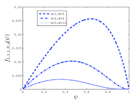
Figure 1: The curves of $f_{1,1,1,N,d}(\cdot)$.

If the conditions of Lemma V.1 hold, then $F(k)$ is invertible a.s. Thus, by (22), we have

$$F(k) = I_{Nn}-b(k){\mathcal{D}}_{\mathcal{G}(k)}\otimes I_{n}-a(k){\mathcal{H}}^{T}(k){\mathcal{H}}(k)+b(k)\overline{A}(k,0)-C_{1}(k)$$ (28)

$$= I_{Nn}-b(k){\mathcal{D}}_{\mathcal{G}(k)}\otimes I_{n}-a(k){\mathcal{H}}^{T}(k){\mathcal{H}}(k)+b(k)\overline{A}(k,0)$$ (31)

$$~{}~{}~{}-(C_{2}(k)-b(k)\overline{A}(k,1))F^{-1}(k-1)$$

$$~{}~{}~{}~{}~{}~{}~{}~{}~{}~{}~{}~{}~{}~{}~{}\vdots$$

$$= I_{Nn}-G(k),~{}k\geq 0,$$ (32)

where

$$G(k)\triangleq b(k)\mathcal{\mathcal{D}}_{\mathcal{G}(k)}\otimes I_{n}+a(k){\mathcal{H}}^{T}(k){\mathcal{H}}(k)-b(k)\sum_{q=0}^{d}\overline{A}(k,q)\big{[}\Phi_{F}(k-1,k-q)\big{]}^{-1}.$$ (33)

For any given positive integers $h$ and $m$, denote

$${\widetilde{\Lambda}_{m}^{h}}=\lambda_{\min}\Bigg{[}\sum_{k=mh}^{(m+1)h-1}\Bigg{(}{b(k)}\mathbb{E}[\widehat{\mathcal{L}}_{\mathcal{G}(k)}|\mathcal{F}(mh-1)]\otimes I_{n}+a(k)\mathbb{E}[{\mathcal{H}}^{T}(k){\mathcal{H}}(k)|\mathcal{F}(mh-1)]$$ (34)

$$~{}~{}~{}~{}~{}~{}~{}~{}~{}~{}~{}~{}~{}-\frac{b(k)}{2}\sum_{q=0}^{d}\mathbb{E}\Big{[}\overline{A}(k,q)[[\Phi_{F}(k-1,k-q)]^{-1}-I_{Nn}]$$ (35)

$$~{}~{}~{}~{}~{}~{}~{}~{}~{}~{}~{}~{}~{}+[[\Phi_{F}(k-1,k-q)]^{-1}-I_{Nn}]^{T}\overline{A}^{T}(k,q)\Big{|}\mathcal{F}(mh-1)\Big{]}\Bigg{)}\Bigg{]}.$$ (36)

Theorem V.1.

Suppose that Assumptions A1.a–A1.b, A2.b hold. If Conditions C1.a, C1.d hold, and there exists an integer $h>0$ and a positive real sequence $\{c(m),m\geq 0\}$ with $b^{2}(mh)=o(c(m))$, $\sum_{m=0}^{\infty}c(m)=\infty$, such that

$${\widetilde{\Lambda}_{m}^{h}}\geq c(m)\ \mathrm{a.s.},\ m\geq 0,$$ (37)

then the algorithm (9) converges in mean square.

If $\{\langle\mathcal{H}(k),\mathcal{A}_{\mathcal{G}(k)},\lambda_{ji}(k),j,i\in\mathcal{V}\rangle,k\geq 0\}$ is an independent random process, then Corollary V.1 below gives a sufficient condition for the condition (37) in Theorem V.1 to hold, which is more intuitive and computable.

Corollary V.1.

Suppose that Assumptions A1.a–A1.b, A2.b hold, $\{\langle\mathcal{H}(k),\mathcal{A}_{\mathcal{G}(k)},\lambda_{ji}(k),j,i\in\mathcal{V}\rangle,k\geq 0\}$ is an independent process. If Condition C1.a holds, $b(0)\leq f_{C_{1},\beta_{a},\beta_{H},N,d}(\psi_{2})$ with $\psi_{2}\in(0,{2}^{\frac{1}{d}}-1)$, and there exists an integer $h>0$ and a positive real sequence $\{c(m),m\geq 0\}$ with $b^{2}(mh)=o(c(m))$ and $\sum_{m=0}^{\infty}c(m)=\infty$, such that

$$\overline{\Lambda}_{m}^{h}-\sum_{k=mh}^{(m+1)h-1}\Bigg{[}{b(k)}\sum_{q=0}^{d}\frac{\|\mathbb{E}[\overline{A}(k,q)]\|[(1+\psi_{2})^{q}-1]}{2-(1+\psi_{2})^{q}}\Bigg{]}\geq c(m),\ m\geq 0,$$ (38)

then the algorithm (9) converges in mean square.

Next, for the case with conditionally balanced digraphs, the following corollary presents a more intuitive convergence condition.

Corollary V.2.

Suppose that Assumptions A1.a–A1.b, A2.b hold and $\{\mathcal{G}(k),k\geq 0\}\in\Gamma_{1}$. If Conditions C1.a–C1.b, C1.d hold, $b(k)=O(a(k))$, and there exists an integer $h>0$, a constant $\theta>0$ such that

$$\inf_{m\geq 0}(\Lambda_{m}^{h}-\Sigma_{m}^{h})\geq\theta\ \mathrm{a.s.}$$ (39)

where

$$\Sigma_{m}^{h}=C_{2}(C_{3})^{h}\max\{1,C_{1}\}\sum_{k=mh}^{(m+1)h-1}\sum_{q=0}^{d}\|\mathbb{E}[\overline{A}(k,q)([\Phi_{F}(k-1,k-q)]^{-1}-I_{Nn})|\mathcal{F}(mh-1)]\|$$

with $C_{2}\triangleq\sup_{k\geq 0}\frac{b(k)}{a(k)}$ and $C_{3}\triangleq\sup_{k\geq 0}\frac{a(k)}{a(k+1)}$, then, the algorithm (9) converges in mean square. Furthermore, if $\{\langle\mathcal{H}(k),\mathcal{A}_{\mathcal{G}(k)},\lambda_{ji}(k),j,i\in\mathcal{V}\rangle,k\geq 0\}$ is an independent process, then (39) holds if there exist an integer $h>0$ such that

$$\inf_{m\geq 0}\Lambda_{m}^{h}>C_{2}(C_{3})^{h}\max\{1,C_{1}\}\sup_{m\geq 0}\Bigg{[}\sum_{k=mh}^{(m+1)h-1}\sum_{q=0}^{d}\|\mathbb{E}[\overline{A}(k,q)]\|\frac{[(1+\psi_{2})^{q}-1]}{2-(1+\psi_{2})^{q}}\Bigg{]},$$ (40)

and $b(0)\leq f_{C_{1},\beta_{a},\beta_{H},N,d}(\psi_{2})$, with $\psi_{2}\in(0,{2}^{\frac{1}{d}}-1)$, where $C_{1}$ is defined in Condition C1.d.

Remark 8.

Theorem V.1, Corollaries V.1-V.2 give explicit convergence conditions under which all nodes’ estimates converge to the true parameter in mean square. Existing literature used the Lyapunov-Krasovskii functional method to deal with time delays and obtained the non-explicit LMI type convergence condition ([30]). In contrast, here, we transform the system with random time-varying communication delays into an equivalent delay-free system by introducing an auxiliary system and then adopt the method of binomial expansion of random matrix products to transform the mean square convergence analysis of the delay-free system into that of the mathematical expectation of random matrix products, and obtain the key convergence conditions (37)-(39) which explicitly rely on the conditional expectations of delay matrices, observation matrices and weighted adjacency matrices of communication graphs over a sequence of fixed-length time intervals. In the absence of time delays, the condition (37) degenerates to the condition (b.1) in Theorem IV.1.

Remark 9.

The conditions (38) and (40) can be further simplified for special delay processes. If the delays are independent of the graphs, then $\mathbb{E}[\overline{A}(k,q)]=\mathbb{E}[\mathcal{A}_{\mathcal{G}(k)}]\circ\mathbb{E}[\mathcal{I}(k,q)]$. Here, the element in the $i$th row and the $j$th column of $\mathbb{E}[\mathcal{I}(k,q)]$, $\mathbb{E}[\mathcal{I}(k,q)]_{ij}=\mathbb{P}\{\lambda_{ji}(k)=q\}=p_{ji,q}(k)$. In addition,

• if $\lambda_{ji}(k)$ are identically distributed w.r.t. $k$, then $\mathbb{E}[\mathcal{I}(k,q)]_{ij}=p_{ji,q}(0),\forall~{}k\geq 0$;

• if $\lambda_{ji}(k)$ are identically distributed w.r.t. both $k$ and $(j,i)$, then $\mathbb{E}[\mathcal{I}(k,q)]_{ij}=p_{q},i\not=j$ where $p_{q}$ denotes the probability that the packet is delayed by $q$ steps for all $k$ and $(j,i),j\not=i$. Therefore, $\|\mathbb{E}[\overline{A}(k,q)]\|=p_{q}\|\mathbb{E}[\mathcal{A}_{\mathcal{G}(k)}]\|$. Furthermore, if the graph sequence is an i.i.d. process, then the condition (40) becomes

  $$\inf_{m\geq 0}\Lambda_{m}^{h}>C_{2}(C_{3})^{h}\max\{1,C_{1}\}h\|\mathbb{E}[\mathcal{A}_{\mathcal{G}(0)}]\|\sum_{q=0}^{d}\frac{p_{q}[(1+\psi_{2})^{q}-1]}{2-(1+\psi_{2})^{q}}.$$

Corollaries V.1-V.2 show that for given algorithm gains $\{a(k),k\geq 0\}$ and $\{b(k),k\geq 0\}$, if the communication graphs and observation matrices are persistently excited with enough intensity, then the additional effects of time delays can be mitigated. The maximum delay bound $d$ that can be allowed is related to the weighted adjacency matrix of mean graphs $\mathbb{E}[\mathcal{A}_{\mathcal{G}(k)}]$, the probability distribution of time delays $\mathbb{E}[\mathcal{I}(k,q)]$ and the algorithm gains. In the absence of time delays, (39) degenerates to the condition (c.1) in Theorem IV.2. The following corollary shows that for the case with conditionally balanced graphs, if the stochastic spatio-temporal persistence of excitation condition $\inf_{m\geq 0}{{\Lambda_{m}^{h}}}\geq\theta$ a.s. holds, then for any given bounded delays, mean square convergence of the algorithm can be guaranteed if the algorithms gains are properly designed and sufficiently small.

Corollary V.3.

Suppose that Assumptions A1.a–A1.b, A2.b hold, $\{\mathcal{G}(k),k\geq 0\}\in\Gamma_{1}$ and there exists an integer $h>0$, a constant $\theta>0$ such that $\inf_{m\geq 0}{{\Lambda_{m}^{h}}}\geq\theta$ a.s. If Conditions C1.a–C1.b hold, $b(k)=O(a(k))$, and $b(0)\leq f_{C_{1},\beta_{a},\beta_{H},N,d}(\psi_{3})$ with $\psi_{3}\in(0,(1+{\theta}/[{\theta+{N}C_{2}(C_{3})^{h}\max\{1,C_{1}\}\beta_{a}dh}])^{\frac{1}{d}}-1)$, then the algorithm (9) converges in mean square.

VI numerical example

We apply our algorithm to decentralized multi-area online state estimation in power systems to illustrate the effectiveness of the obtained theoretical results. An IEEE 14-bus system is used for the test, which has 14 buses and is partitioned into 4 areas $A_{1},A_{2},A_{3},A_{4}$, shown in Figure 2. After a DC power flow approximation ([34]), the grid state to be estimated degenerates into a vector of voltage phase angles at all buses. Let bus 1’s voltage phase angle be zero, as the reference bus. The grid state to be estimated is given by

$$x_{0}=[-4.98,-12.72,-11.33,-8.78,-14.22,-13.37,$$

$$~{}~{}~{}~{}~{}~{}~{}~{}~{}~{}~{}~{}~{}~{}~{}~{}~{}~{}~{}~{}~{}~{}~{}-13.36,-14.94,-15.10,-14.79,-15.05,-15.12,-16.03]^{T}.$$

The measurements $z_{i}(k)$ are linearly related to $x_{0}$, given by $z_{i}(k)=s_{i}(k)H_{i}^{\prime}x_{0}+v_{i}(k),\ i=1,2,3,4,$ where the noise $\{v_{i}(k),k\geq 0\}$ is assumed to be an i.i.d. process with the standard normal distribution, $\{s_{i}(k),k\geq 0\}$ is an i.i.d. sequence, modelling the sensing failures with $\mathbb{P}\{s_{i}(k)=1\}=\mathbb{P}\{s_{i}(k)=0\}=0.5$, and $H_{i}^{\prime}$, $i=1,...,4$ are the observation matrices, which are deterministic and given in Appendix D. There are $4$ random communication links with $0-1$ weights, represented by the red dotted lines in Figure 2. At odd time instants, the link from $A_{2}$ to $A_{3}$ awakes with the probability $0.5$ and the others sleep; at even time instants, the link from $A_{2}$ to $A_{3}$ sleeps and the others awake with the probability $0.5$. Both $\{\mathcal{G}(k),k\geq 0\}$ and $\{H(k),k\geq 0\}$ are independent processes. We use the averaged relative error, $\frac{\sum_{i=1}^{4}\|x_{i}(k)-x_{0}\|}{4\|x_{0}\|}$, to evaluate the performance of the algorithm.

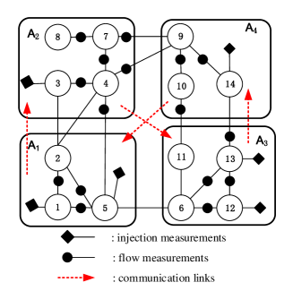
Figure 2: IEEE-14 multi-area buses and the communication graphs.

For the delay-free case, set $a(k)=b(k)=\frac{0.5}{(k+1)^{0.52}}$. Let $c(m)=\frac{0.0112}{(2m+2)^{0.52}}$. When $h=2$, we plot the curves of $\overline{\Lambda}_{m}^{2}$ and $c(m)$ w.r.t. $m$ in Figure 4, which shows that $\overline{\Lambda}_{m}^{2}\geq c(m),m\geq 0$. The conditions of Theorem IV.1 hold. Figure 4 is depicted with the curves of the averaged relative errors, where the red line represents the error curve of the algorithm without random link failures and sensing failures, as the base case. It shows that in spite of the unbalance of the mean graphs and the sensing failures, the four areas’ estimates converge to $x_{0}$.

For the case with time delays, assume that the delays are independent of the communication graphs, observation matrices and measurement noises, and subjected to the Bernoulli distribution, i.e. $\lambda_{ji}(k)\sim B(d,p)$ for all $k$ and $(j,i)$. Then

$$\mathbb{P}\{\lambda_{ji}(k)=q\}=\mathbb{C}_{d}^{q}p^{q}(1-p)^{d-q},q=0,\cdots,d.$$ (41)

Set $d=4,p=0.4$. We now verify the convergence conditions in Corollary V.1. Let $a(k)=b(k)$. Then $C_{1}=1$. By the above settings of communication graphs and measurement matrices, we know that $\beta_{a}=1$,$\beta_{H}=4.07$. Let $\psi_{2}=0.01$. Then we have $f_{C_{1},\beta_{a},\beta_{H},N,d}(\psi_{2})=0.0005$. Then, let $b(k)=\frac{0.0005}{(k+1)^{0.1}}$. By the definition of $p_{q}$ in Remark 9, it follows from (41) that $p_{q}=\mathbb{C}_{4}^{q}0.4^{q}0.6^{4-q},q=0,...,4$. Note that $\|\mathbb{E}[\mathcal{A}_{\mathcal{G}(k)}]\|\equiv 0.5$. As is discussed in Remark 9, $\|\mathbb{E}[\overline{A}(k,q)]\|=p_{q}\|\mathbb{E}[\mathcal{A}_{\mathcal{G}(k)}]\|$. Hence, it can be calculated that

$$\sum_{k=mh}^{(m+1)h-1}b(k)\sum_{q=0}^{d}\|\mathbb{E}[\overline{A}(k,q)]\|\frac{[(1+\psi_{2})^{q}-1]}{2-(1+\psi_{2})^{q}} = \sum_{k=2m}^{2m+1}b(k)\sum_{q=0}^{4}\frac{0.5p_{q}[(1+\psi_{2})^{q}-1]}{2-(1+\psi_{2})^{q}}$$

$$= 0.01\sum_{k=2m}^{2m+1}b(k).$$

Note that $\overline{\Lambda}_{m}^{2}=\lambda_{\min}[\sum_{k=2m}^{2m+1}b(k)(\mathbb{E}[\widehat{\mathcal{L}}_{\mathcal{G}(k)}]\otimes I_{13}+\mathbb{E}[{\mathcal{H}}^{T}(k){\mathcal{H}}(k)])]$. Let $c(m)=\frac{0.00001}{(4m+4)^{0.1}}$. We plot the curves of $\overline{\Lambda}_{m}^{2}-0.01\sum_{k=2m}^{2m+1}b(k)$ and $c(m)$ w.r.t. $m$ in Figure 6, showing that the condition (38) in Corollary V.1 holds. Figure 6 is depicted with curve of the averaged relative error, which confirms Corollary V.1.

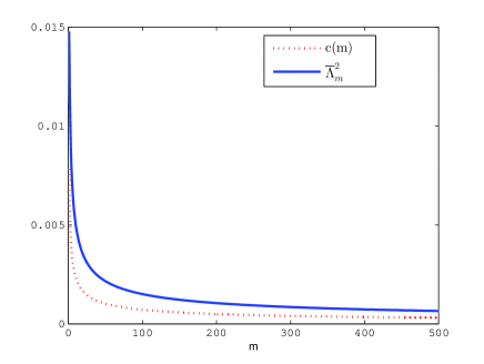
Figure 3: Curves of ${\overline{\Lambda}_{m}^{2}}$ and $c(m)=\frac{0.0112}{(2m+2)^{0.52}}$ w.r.t. $m$.

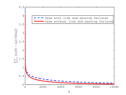
Figure 4: Curves of the averaged relative error $\frac{\sum_{i=1}^{4}\|x_{i}(k)-x_{0}\|}{4\|x_{0}\|}$ for the delay-free case.

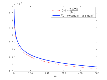
Figure 5: Curves of $\overline{\Lambda}_{m}^{2}-0.01\sum_{k=2m}^{2m+1}b(k)$ and $c(m)$ w.r.t. $m$.

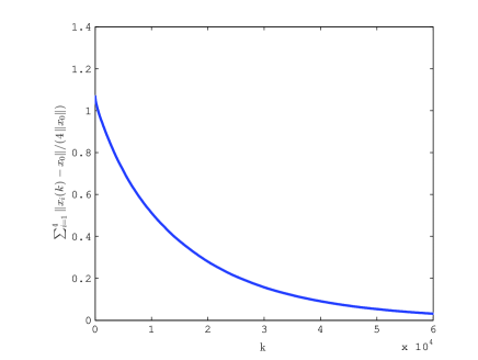
Figure 6: Curve of the averaged relative error for the case with random time delays.

VII conclusion

In this paper, we analyzed the convergence of the decentralized cooperative online parameter estimation algorithm in an uncertain communication environment. Each node has a partial linear observation of the unknown parameter with random time-varying observation matrices. The underlying communication network is modeled by a sequence of random digraphs and is subjected to nonuniform random time-varying delays in channels. For the delay-free case, we proved that if the observation matrices and the graph sequence satisfy the stochastic spatio-temporal persistence of excitation condition, then the algorithm gains can be designed properly such that all nodes’ estimates converge to the true parameter in mean square and almost surely. Specially, for Markovian switching communication graphs and observation matrices, this condition holds if the stationary graph is balanced with a spanning tree and the measurement model is spatio-temporally jointly observable. For the case with communication delays, we introduced delay matrices to model the random time-varying communication delays, adopted the method of binomial expansion of random matrix products to transform the mean square convergence analysis of the algorithm into that of the mathematical expectation of random matrix products, and obtained mean square convergence conditions explicitly relying on the conditional expectations of delay matrices, observation matrices and weighted adjacency matrices of communication graphs over a sequence of fixed-length intervals. In the absence of time delays, these mean square convergence conditions degenerate to the stochastic spatio-temporal persistence of excitation conditions. Especially, given that the digraphs are conditionally balanced, we show that if the stochastic spatio-temporal persistence of excitation condition holds, then for any given bounded delay, proper algorithm gains can be designed to guarantee mean square convergence of the algorithm.

There are many interesting open issues for future research. Theorem V.1 is established for a very general type of delays, namely random and unordered. This means that in the practical implementation, the packets of information exchanged by pairs of nodes are being placed in a processing queue without any regard to their transmit time stamp. In some cases, all received packets are ordered by the time stamp of their transmission, and the communication delays would be random and monotone ([32],[44],[45]). How to explore monotonicity constraints in the random delay process to relax the conditions or strengthen the results of Theorem V.1 would be an interesting and challenging issue. The main obstacle is how to deal with the delay-induced products of the inverse of matrices, which is difficult and may need more advanced techniques. Another important issue is the convergence rate of the algorithm. Especially, Corollary V.3 shows that for the case with conditionally balanced graphs, if the stochastic spatio-temporal persistence of excitation condition holds, then for any given bounded delays, mean square convergence of the algorithm can be guaranteed if we choose sufficiently small algorithms gains. However, smaller algorithm gains generally lead to a slower convergence. Thus, how to choose the algorithms gains for optimizing the convergence rate is an interesting topic for future investigation.

Appendix A several useful lemmas

Definition A.1.

([39]) A Markov chain on a countable state space $\mathcal{S}$ with a stationary distribution $\pi$ and transition function $\mathbb{P}(x,\cdot)$ is called uniform ergodic, if there exist positive constants $r>1$ and $R$ such that for all $x\in\mathcal{S}$, $\|\mathbb{P}^{n}(x,\cdot)-\pi\|\leq Rr^{-n}$. Here, $\|\mathbb{P}^{n}(x,\cdot)-\pi\|=\sum_{y}|\mathbb{P}^{n}(x,y)-\pi_{y}|$.

Lemma A.1.

([40]) For any given matrix $P$, denote $W=I-P$. If there exists a constant $\psi\in(0,1)$ such that $\|P\|\leq\psi$, then $W$ is invertible and $\|W^{-1}\|\leq(1-\|P\|)^{-1}\leq(1-\psi)^{-1}.$

Lemma A.2.

([41]) Assume that $\{s_{1}(k),k\geq 0\}$ and $\{s_{2}(k),k\geq 0\}$ are real sequences satisfying $0\leq s_{2}(k)<1$, $\sum_{k=0}^{\infty}s_{2}(k)=\infty$ and $\lim_{k\to\infty}\frac{s_{1}(k)}{s_{2}(k)}$ exists. Then

$$\lim_{k\to\infty}\sum_{i=1}^{k}s_{1}(i)\prod_{l=i+1}^{k}(1-s_{2}(l))=\lim_{k\to\infty}\frac{s_{1}(k)}{s_{2}(k)}.$$

Lemma A.3.

([42]) Assume that $\{x(k),\mathcal{F}(k)\},~{}\{\alpha(k),\mathcal{F}(k)\},~{}\{\beta(k),\mathcal{F}(k)\}~{}\mathrm{and}~{}\{\gamma(k),\mathcal{F}(k)\}$ are all nonnegative adaptive sequences, satisfying

$$\mathbb{E}[x(k+1)|\mathcal{F}(k)]\leq(1+\alpha(k))x(k)-\beta(k)+\gamma(k),k\geq 0~{}\rm{a.s.}$$

If $\sum_{k=0}^{\infty}(\alpha(k)+\gamma(k))<\infty~{}\rm{a.s.}$, then $x(k)$ converges to a finite random variable a.s. and $\sum_{k=0}^{\infty}\beta(k)<\infty~{}\rm{a.s.}$

For the subsequent Lemmas A.4 and A.5, the readers may be referred to Theorem 6.4 and its next paragraph in Ch. 6 of [43].

Lemma A.4.

(Conditional Lyapunov inequality) Denote the probability space by $(\Psi,\mathcal{F},P)$. Let $\mathcal{F}_{1}$ be a sub $\sigma-$algebra of $\mathcal{F}$ and $\xi$ be a random variable on $(\Psi,\mathcal{F},P)$. Then $(\mathbb{E}[|\xi|^{s}|\mathcal{F}_{1}])^{\frac{1}{s}}\leq(\mathbb{E}[|\xi|^{t}|\mathcal{F}_{1}])^{\frac{1}{t}}~{}\mathrm{a.s.},~{}0<s<t.$

Lemma A.5.

(Conditional Hölder inequality) Denote the probability space $(\Psi,\mathcal{F},P)$. Let $\mathcal{F}_{1}$ be a sub $\sigma-$algebra of $\mathcal{F}$. Let $\xi$ and $\eta$ be two random variables on $(\Psi,\mathcal{F},P)$. Let constants $p\in(1,\infty),~{}q\in(1,\infty)$ and $1/p+1/q=1$. If $\mathbb{E}[|\xi|^{p}]<\infty$ and$~{}\mathbb{E}[|\eta|^{q}]<\infty$, then $\mathbb{E}[|\xi\eta||\mathcal{F}_{1}]\leq(\mathbb{E}[|\xi|^{p}|\mathcal{F}_{1}])^{\frac{1}{p}}(\mathbb{E}[|\eta|^{q}|\mathcal{F}_{1}])^{\frac{1}{q}}~{}\rm{a.s.}$

Lemma A.6.

For any random matrix $A\in\mathbb{R}^{m\times n}$, $\|\mathbb{E}[AA^{T}]\|\leq n\|\mathbb{E}[A^{T}A]\|$.

Proof.

By the properties of matrix trace, we have $\|\mathbb{E}[AA^{T}]\|=\lambda_{\max}(\mathbb{E}[AA^{T}])\leq\mathrm{Tr}(\mathbb{E}[AA^{T}])=\mathrm{Tr}(\mathbb{E}[A^{T}A])\leq n\lambda_{\max}(\mathbb{E}[A^{T}A])=n\|\mathbb{E}[A^{T}A]\|$. ∎

Lemma A.7.

Let $\mathcal{A}=[a_{ij}]_{N\times N}$ be a weighted adjacency matrix of an undirected graph with $N$ nodes and $\mathcal{L}$ be the associated Laplacian matrix. Let $x=[x^{T}_{1},...,x_{N}^{T}]^{T}\in\mathbb{R}^{Nn}$ be any given nonzero $Nn$-dimensional vector where $x_{i}\in\mathbb{R}^{n}$, $i=1,2,...,N$ and there exists $i\neq j$, such that $x_{i}\neq x_{j}$. If $a_{ij}\geq 0$, $i,j=1,2,...,N$ and the graph is connected, then $x^{T}(\mathcal{L}\otimes I_{n})x>0$.

Proof.

By the definition of Laplacian matrix, we have $x^{T}(\mathcal{L}\otimes I_{n})x=\frac{1}{2}\sum_{i=1}^{N}\sum_{j=1}^{N}a_{ij}\|x_{i}-x_{j}\|^{2}$. Noting that there exists $i\neq j$, such that $x_{i}\neq x_{j}$ and the graph is connected, by $a_{ij}\geq 0$, $i,j=1,2,...,N$, we get $x^{T}(\mathcal{L}\otimes I_{n})x>0$. ∎

Appendix B proofs in Section IV

Let

$$P(k)=I_{Nn}-D(k),$$ (42)

where

$$D(k)=b(k)\mathcal{L}_{\mathcal{G}(k)}\otimes I_{n}+a(k){\mathcal{H}}^{T}(k){\mathcal{H}}(k).$$ (43)

The proof of Theorem IV.1 needs the following lemma.

Lemma B.1.

For the algorithm (9), if Condition C1.a, the conditions (b.1) and (b.2) in Theorem IV.1 hold, then

$$\lim_{k\to\infty}\|\mathbb{E}[\Phi_{P}(k,0)\Phi_{P}^{T}(k,0)]\|=0.$$ (44)

Proof.

By (42), we have

$$\Phi^{T}_{P}((m+1)h-1,mh)\Phi_{P}((m+1)h-1,mh)$$ (45)

$$= (I_{Nn}-D^{T}(mh))\cdots(I_{Nn}-D^{T}((m+1)h-1))$$ (47)

$$\times(I_{Nn}-D((m+1)h-1))\cdots(I_{Nn}-D(mh)).$$

Taking conditional expectation w.r.t. $\mathcal{F}(mh-1)$ on both sides of the above, by the binomial expansion, we have

$$~{}~{}~{}\|\mathbb{E}[\Phi^{T}_{P}((m+1)h-1,mh)\Phi_{P}((m+1)h-1,mh)|\mathcal{F}(mh-1)]\|$$ (48)

$$=\|\mathbb{E}[(I_{Nn}-D^{T}(mh))\cdots(I_{Nn}-D^{T}((m+1)h-1))$$ (49)

$$~{}\times(I_{Nn}-D((m+1)h-1))\cdots(I_{Nn}-D(mh))|\mathcal{F}(mh-1)]\|$$ (50)

$$=\Big{\|}I_{Nn}-\sum_{k=mh}^{(m+1)h-1}\mathbb{E}[D^{T}(k)+D(k)|\mathcal{F}(mh-1)]$$ (51)

$$~{}+\mathbb{E}[M_{2}(m)+\cdots+M_{2h}(m)|\mathcal{F}(mh-1)]\Big{\|}$$ (52)

$$\leq\Big{\|}I_{Nn}-\sum_{k=mh}^{(m+1)h-1}\mathbb{E}[D^{T}(k)+D(k)|\mathcal{F}(mh-1)]\Big{\|}$$ (53)

$$~{}+\left\|\mathbb{E}[M_{2}(m)+\cdots+M_{2h}(m)|\mathcal{F}(mh-1)]\right\|.$$ (54)

Here, $M_{i}(m),i=2,\cdots,2h$ represent the $i$-th order terms in the binomial expansion of $\Phi_{P}((m+1)h-1,mh)\Phi_{P}^{T}((m+1)h-1,mh)$.

Since the 2-norm of a symmetric matrix is equal to its spectral radius, by the definition of spectral radius, we have

$$~{}~{}~{}\Big{\|}I_{Nn}-\sum_{k=mh}^{(m+1)h-1}\mathbb{E}[D(k)+D^{T}(k)|\mathcal{F}(mh-1)]\Big{\|}$$ (55)

$$=\rho\Bigg{(}I_{Nn}-\sum_{k=mh}^{(m+1)h-1}\mathbb{E}[D(k)+D^{T}(k)|\mathcal{F}(mh-1)]\Bigg{)}$$ (56)

$$=\max_{1\leq i\leq Nn}\Bigg{|}\lambda_{i}\Bigg{(}I_{Nn}-\sum_{k=mh}^{(m+1)h-1}\mathbb{E}[D(k)+D^{T}(k)|\mathcal{F}(mh-1)]\Bigg{)}\Bigg{|}$$ (57)

$$=\max_{1\leq i\leq Nn}\Bigg{|}1-\lambda_{i}\Bigg{(}\sum_{k=mh}^{(m+1)h-1}\mathbb{E}[D(k)+D^{T}(k)|\mathcal{F}(mh-1)]\Bigg{)}\Bigg{|}.$$ (58)

Since both $a(k)$ and $b(k)$ tend to zero, by the condition (b.2), we know that there exists a positive integer $m_{1}$, which is independent of the sample paths, such that

$$\lambda_{i}\Bigg{(}\sum_{k=mh}^{(m+1)h-1}\mathbb{E}[D(k)+D^{T}(k)|\mathcal{F}(mh-1)]\Bigg{)}\leq 1,~{}i=1,\cdots,Nn,~{}\forall~{}m\geq m_{1}~{}\rm{a.s.}$$

This together with (48) and (55) leads to

$$~{}~{}~{}\|\mathbb{E}[\Phi_{P}^{T}((m+1)h-1,mh)\Phi_{P}((m+1)h-1,mh)|\mathcal{F}(mh-1)]\|$$ (59)

$$\leq 1-\lambda_{\min}\Bigg{(}\sum_{k=mh}^{(m+1)h-1}\mathbb{E}[D(k)+D^{T}(k)|\mathcal{F}(mh-1)]\Bigg{)}$$ (60)

$$~{}+\left\|\mathbb{E}[M_{2}(m)+\cdots+M_{2h}(m)|\mathcal{F}(mh-1)]\right\|,~{}\forall~{}m\geq m_{1}~{}\rm{a.s.}$$ (61)

We next bound the two terms on the right side of the above. For the first term, by the definitions of $D(k)$ and $\overline{\Lambda}_{m}^{h}$ and the condition (b.1), we have

$$~{}~{}~{}1-\lambda_{\min}\Bigg{(}\sum_{k=mh}^{(m+1)h-1}\mathbb{E}[D(k)+D^{T}(k)|\mathcal{F}(mh-1)]\Bigg{)}$$ (62)

$$=1-\lambda_{\min}\Bigg{(}\sum_{k=mh}^{(m+1)h-1}\mathbb{E}[2b(k)\widehat{\mathcal{L}}_{\mathcal{G}(k)}\otimes I_{n}+2a(k){\mathcal{H}}^{T}(k){\mathcal{H}}(k)|\mathcal{F}(mh-1)]\Bigg{)}$$ (63)

$$=1-2\overline{\Lambda}_{m}^{h}$$ (64)

$$\leq 1-c(m),~{}\forall~{}m\geq m_{1}~{}\rm{a.s.}$$ (65)

By Lemma A.4 and the condition (b.2), it follows that

$$\sup_{k\geq 0}\mathbb{E}[\|\widetilde{D}(k)\|^{i}|\mathcal{F}(k-1)]\leq\sup_{k\geq 0}[\mathbb{E}[\|\widetilde{D}(k)\|^{2^{h}}|\mathcal{F}(k-1)]]^{\frac{i}{2^{h}}}\leq\rho_{0}^{i}~{}\mathrm{a.s.},~{}2\leq i\leq 2^{h},$$

where $\widetilde{D}(k)=\mathcal{L}_{\mathcal{G}(k)}\otimes I_{n}+{\mathcal{H}}^{T}(k){\mathcal{H}}(k)$. Note that for any given random variable $\xi$ and $\sigma$-algebra $\mathcal{F}_{1}\subseteq\mathcal{F}_{2},$ it is true that

$$\mathbb{E}[\xi|\mathcal{F}_{1}]=\mathbb{E}[\mathbb{E}[\xi|\mathcal{F}_{2}]|\mathcal{F}_{1}].$$ (66)

We then have

$$\mathbb{E}[\|\widetilde{D}(k)\|^{l}|\mathcal{F}(mh-1)]=\mathbb{E}[\mathbb{E}[\|\widetilde{D}(k)\|^{l}|\mathcal{F}(k-1)]|\mathcal{F}(mh-1)],~{}2\leq l\leq 2^{h},~{}k\geq mh.$$

From the definitions of $M_{i}(m),i=2,\cdots,2h$ and the above, by termwise multiplication and using Lemma A.5 repeatedly, for the second term on the right side of (59), we have

$$\|\mathbb{E}[M_{2}(m)+\cdots+M_{2h}(m)|\mathcal{F}(mh-1)]\| \leq b^{2}(mh)\Bigg{(}\sum_{i=2}^{2h}\mathbb{C}_{2h}^{i}(\max\{1,\phi\}\rho_{0})^{i}\Bigg{)}$$ (67)

$$= b^{2}(mh)\alpha,$$ (68)

where $\phi$ satisfies $a(k)\leq\phi b(k)$, $\alpha=(1+\max\{1,\phi\}\rho_{0})^{2h}-1-2h\max\{1,\phi\}\rho_{0}$ and $\mathbb{C}_{m}^{p}$ denotes the combinatorial number of choosing $p$ elements from $m$ elements. By (59)-(67), we have

$$~{}~{}~{}\|\mathbb{E}[\Phi_{P}^{T}((m+1)h-1,mh)\Phi_{P}((m+1)h-1,mh)|\mathcal{F}(mh-1)]\|$$ (69)

$$\leq 1-c(m)+b^{2}(mh)\alpha,~{}m\geq m_{1}~{}\rm{a.s.}$$ (70)

Denote $m_{k}=\lfloor\frac{k}{h}\rfloor$. By the properties of the conditional expectation, Lemma A.6 and (69), we have

$$~{}~{}~{}\|\mathbb{E}[\Phi_{P}(k,0)\Phi_{P}^{T}(k,0)]\|$$ (71)

$$\leq Nn\|\mathbb{E}[\Phi_{P}^{T}(k,0)\Phi_{P}(k,0)]\|$$ (72)

$$=Nn\|\mathbb{E}[\Phi_{P}^{T}(m_{k}h-1,0)\Phi_{P}^{T}(k,m_{k}h)\Phi_{P}(k,m_{k}h)\Phi_{P}(m_{k}h-1,0)]\|$$ (73)

$$\leq Nn\|\mathbb{E}[\Phi_{P}^{T}(m_{k}h-1,0)\|\Phi_{P}^{T}(k,m_{k}h)\Phi_{P}(k,m_{k}h)\|\Phi_{P}(m_{k}h-1,0)]\|$$ (74)

$$=Nn\|\mathbb{E}[\mathbb{E}[\Phi_{P}^{T}(m_{k}h-1,0)\|\Phi_{P}^{T}(k,m_{k}h)\Phi_{P}(k,m_{k}h)\|\Phi_{P}(m_{k}h-1,0)|\mathcal{F}(m_{k}h-1)]]\|$$ (75)

$$=Nn\|\mathbb{E}[\Phi_{P}^{T}(m_{k}h-1,0)\mathbb{E}[\|\Phi_{P}^{T}(k,m_{k}h)\Phi_{P}(k,m_{k}h)\||\mathcal{F}(m_{k}h-1)]$$ (76)

$$~{}\times\Phi_{P}(m_{k}h-1,0)]\|,$$ (77)

For any positive integers $m,n$ satisfying $0\leq m-n\leq h-1,$ it follows from the condition (b.2) that there exists a constant $\rho^{*}_{h}>0$ such that

$$\|\mathbb{E}[\Phi_{P}^{T}(m,n)\Phi_{P}(m,n)|\mathcal{F}(n-1)]\|<\rho^{*}_{h}\mathrm{a.s.}$$ (78)

By the above and (71), noting that $k-m_{k}h\leq h-1$, we have

$$~{}~{}~{}\|\mathbb{E}[\Phi_{P}(k,0)\Phi_{P}^{T}(k,0)]\|~{}~{}~{}~{}~{}~{}~{}~{}~{}~{}~{}~{}~{}~{}~{}~{}~{}~{}~{}~{}~{}~{}$$ (79)

$$\leq\rho^{*}_{h}Nn\|\mathbb{E}[\Phi_{P}^{T}(m_{k}h-1,0)\Phi_{P}(m_{k}h-1,0)]\|$$ (80)

$$=\rho^{*}_{h}Nn\|\mathbb{E}[\Phi_{P}^{T}(m_{1}h-1,0)\Phi_{P}^{T}(m_{k}h-1,m_{1}h)\Phi_{P}(m_{k}h-1,m_{1}h)\Phi_{P}(m_{1}h-1,0)]\|$$ (81)

$$=\rho^{*}_{h}Nn\|\mathbb{E}[\mathbb{E}(\Phi_{P}^{T}(m_{1}h-1,0)\Phi_{P}^{T}(m_{k}h-1,m_{1}h)$$ (82)

$$~{}\times\Phi_{P}(m_{k}h-1,m_{1}h)\Phi_{P}(m_{1}h-1,0)|\mathcal{F}(m_{1}h-1))]\|$$ (83)

$$\leq\rho^{*}_{h}Nn\|\mathbb{E}[\Phi_{P}^{T}(m_{1}h-1,0)$$ (84)

$$~{}\times\|\mathbb{E}[\Phi_{P}^{T}(m_{k}h-1,m_{1}h)\Phi_{P}(m_{k}h-1,m_{1}h)|\mathcal{F}(m_{1}h-1)]\|\Phi_{P}(m_{1}h-1,0)]\|.$$ (85)

By (66) and (69), we have

$$~{}~{}~{}\|\mathbb{E}[\Phi_{P}^{T}(m_{k}h-1,m_{1}h)\Phi_{P}(m_{k}h-1,m_{1}h)|\mathcal{F}(m_{1}h-1)]\|~{}~{}~{}~{}~{}~{}~{}~{}~{}~{}~{}~{}~{}~{}~{}~{}$$ (86)

$$=\|\mathbb{E}[\Phi_{P}^{T}((m_{k}-1)h-1,m_{1}h)\Phi_{P}^{T}(m_{k}h-1,(m_{k}-1)h)\Phi_{P}(m_{k}h-1,(m_{k}-1)h)$$ (87)

$$~{}~{}~{}~{}~{}~{}\times\Phi_{P}((m_{k}-1)h-1,m_{1}h)|\mathcal{F}(m_{1}h-1)]\|$$ (88)

$$=\|\mathbb{E}[\mathbb{E}[\Phi_{P}^{T}((m_{k}-1)h-1,m_{1}h)\Phi_{P}^{T}(m_{k}h-1,(m_{k}-1)h)\Phi_{P}(m_{k}h-1,(m_{k}-1)h)$$ (89)

$$~{}~{}~{}~{}~{}~{}\times\Phi_{P}((m_{k}-1)h-1,m_{1}h)|\mathcal{F}((m_{k}-1)h-1)]|\mathcal{F}(m_{1}h-1)]\|$$ (90)

$$=\|\mathbb{E}[\Phi_{P}^{T}((m_{k}-1)h-1,m_{1}h)$$ (91)

$$~{}~{}~{}~{}~{}~{}\times\mathbb{E}[\Phi_{P}^{T}(m_{k}h-1,(m_{k}-1)h)\Phi_{P}(m_{k}h-1,(m_{k}-1)h)|\mathcal{F}((m_{k}-1)h-1)]$$ (92)

$$~{}~{}~{}~{}\times\Phi_{P}((m_{k}-1)h-1,m_{1}h)|\mathcal{F}(m_{1}h-1)]\|$$ (93)

$$\leq\|\mathbb{E}[\Phi_{P}^{T}((m_{k}-1)h-1,m_{1}h)$$ (94)

$$~{}~{}~{}~{}\times\|\mathbb{E}[\Phi_{P}^{T}(m_{k}h-1,(m_{k}-1)h)\Phi_{P}(m_{k}h-1,(m_{k}-1)h)|\mathcal{F}((m_{k}-1)h-1)]\|$$ (95)

$$~{}~{}~{}~{}\times\Phi_{P}((m_{k}-1)h-1,m_{1}h)|\mathcal{F}(m_{1}h-1)]\|$$ (96)

$$\leq[1-c(m_{k}-1)+b^{2}((m_{k}-1)h)\alpha]$$ (97)

$$~{}~{}~{}\times\|\mathbb{E}[\Phi_{P}^{T}((m_{k}-1)h-1,m_{1}h)\Phi_{P}((m_{k}-1)h-1,m_{1}h)|\mathcal{F}(m_{1}h-1)]\|$$ (98)

$$\leq\prod_{s=m_{1}}^{m_{k}-1}[1-c(s)+b^{2}(sh)\alpha]~{}\rm{a.s.},$$ (99)

which together with (79) leads to

$$~{}~{}~{}\|\mathbb{E}[\Phi_{P}(k,0)\Phi_{P}^{T}(k,0)]\|$$ (101)

$$\leq\rho^{*}_{h}Nn\|\mathbb{E}[\Phi_{P}^{T}(m_{1}h-1,0)\Phi_{P}(m_{1}h-1,0)]\|\prod_{s=m_{1}}^{m_{k}-1}[1-c(s)+b^{2}(sh)\alpha].$$

By (18), we know that there exists a positive integer $m_{2}$ such that

$$b^{2}(mh)\alpha\leq\frac{1}{2}c(m),~{}\forall~{}m\geq m_{2},$$ (102)

Let $m_{3}=\max\{m_{2},m_{1}\}$ and $r_{1}=\prod_{s=m_{1}}^{m_{3}-1}[1-c(s)+b^{2}(sh)\alpha]$. By (18) and (102), we have

$$~{}~{}~{}\lim_{k\to\infty}\prod_{s=m_{1}}^{m_{k}-1}[1-c(s)+b^{2}(sh)\alpha]$$ (103)

$$\leq\lim_{k\to\infty}r_{1}\prod_{s=m_{3}}^{m_{k}-1}[1-\frac{1}{2}c(s)]$$ (104)

$$\leq\lim_{k\to\infty}r_{1}\exp\Big{(}-\frac{1}{2}\sum_{s=m_{3}}^{m_{k}-1}c(s)\Big{)}$$ (105)

$$=r_{1}\exp\Big{(}-\frac{1}{2}\sum_{s=m_{3}}^{\infty}c(s)\Big{)}=0.$$ (106)

Since $\|\mathbb{E}[\Phi_{P}^{T}(m_{1}h-1,0)\Phi_{P}(m_{1}h-1,0)]\|<\infty$ by the condition (b.2), (101) and (103), we have (44). The lemma is proved. ∎

Proof of Theorem IV.1.

If $\lambda_{ji}(k)=0$ a.s., $\forall\ j,i\in\mathcal{V}$, $\forall\ k\geq 0$, then by (17), we have

$$e(k+1) = P(k)e(k)+a(k){\mathcal{H}}^{T}(k)v(k)$$ (107)

$$= \Phi_{P}(k,0)e(0)+\sum_{i=0}^{k}a(i)\Phi_{P}(k,i+1){\mathcal{H}}^{T}(i)v(i),~{}k\geq 0.$$ (108)

By the above, we have

$$\mathbb{E}[e(k+1)e^{T}(k+1)] = \mathbb{E}[\Phi_{P}(k,0)e(0)e^{T}(0)\Phi_{P}^{T}(k,0)]$$ (113)

$$+\mathbb{E}\Bigg{[}\Phi_{P}(k,0)e(0)\sum_{i=0}^{k}a(i)[\Phi_{P}(k,i+1){\mathcal{H}}^{T}(i)v(i)]^{T}\Bigg{]}$$

$$+\mathbb{E}\Bigg{[}\sum_{i=0}^{k}a(i)\Phi_{P}(k,i+1){\mathcal{H}}^{T}(i)v(i)[\Phi_{P}(k,0)e(0)]^{T}\Bigg{]}$$

$$+\mathbb{E}\Bigg{[}\Bigg{(}\sum_{i=0}^{k}a(i)\Phi_{P}(k,i+1){\mathcal{H}}^{T}(i)v(i)\Bigg{)}$$

$$\times\Bigg{(}\sum_{i=0}^{k}a(i)\Phi_{P}(k,i+1){\mathcal{H}}^{T}(i)v(i)\Bigg{)}^{T}\Bigg{]}.$$

By Assumptions A1.a and A1.b, we know that the second and third terms on the right side of (113) are both equal to zero. Moreover, from

$$\mathbb{E}[v(i)v^{T}(j)]=\mathbb{E}[\mathbb{E}[v(i)v^{T}(j)|\mathcal{F}(i-1)]]=\mathbb{E}[\mathbb{E}[v(i)|\mathcal{F}(i-1)]v^{T}(j)]=0,~{}\forall~{}i>j,$$ (114)

we have

$$~{}~{}~{}\mathbb{E}\Bigg{[}\Bigg{(}\sum_{i=0}^{k}a(i)\Phi_{P}(k,i+1){\mathcal{H}}^{T}(i)v(i)\Bigg{)}\Bigg{(}\sum_{i=0}^{k}a(i)\Phi_{P}(k,i+1){\mathcal{H}}^{T}(i)v(i)\Bigg{)}^{T}\Bigg{]}$$

$$=\mathbb{E}\Bigg{[}\sum_{i=0}^{k}a^{2}(i)\Phi_{P}(k,i+1){\mathcal{H}}^{T}(i)v(i)v^{T}(i){\mathcal{H}}(i)\Phi_{P}(k,i+1)\Bigg{]}.$$

Substituting the above into (113) and taking the 2-norm leads to

$$~{}~{}~{}\|\mathbb{E}[e(k+1)e^{T}(k+1)]\|$$ (115)

$$\leq\|\mathbb{E}[\Phi_{P}(k,0)\Phi_{P}^{T}(k,0)]\|\|e(0)\|^{2}$$ (116)

$$~{}~{}+\sum_{i=0}^{k}a^{2}(i)\|\mathbb{E}[\Phi_{P}(k,i+1){\mathcal{H}}^{T}(i)v(i)v^{T}(i){\mathcal{H}}(i)\Phi_{P}^{T}(k,i+1)]\|$$ (117)

$$=\|\mathbb{E}[\Phi_{P}(k,0)\Phi_{P}^{T}(k,0)]\|\|e(0)\|^{2}$$ (118)

$$~{}~{}+\sum_{i=k-3h}^{k}a^{2}(i)\|\mathbb{E}[\Phi_{P}(k,i+1){\mathcal{H}}^{T}(i)v(i)v^{T}(i){\mathcal{H}}(i)\Phi_{P}^{T}(k,i+1)]\|$$ (119)

$$~{}~{}+\sum_{i=0}^{k-3h-1}a^{2}(i)\|\mathbb{E}[\Phi_{P}(k,i+1){\mathcal{H}}^{T}(i)v(i)v^{T}(i){\mathcal{H}}(i)\Phi_{P}^{T}(k,i+1)]\|.$$ (120)

By Lemma B.1, we know that the first term in the above converges to zero. For the second term in the above, when $k-h\leq i<k$, we have by (78) that $\|\mathbb{E}[\Phi_{P}^{T}(k,i+1)\Phi_{P}(k,i+1)|\mathcal{F}(i)]\|\leq\rho^{*}_{h}$ a.s.; when $k-2h\leq i<k-h$, it follows from Lemma A.6 and (78) that

$$~{}~{}~{}\|\mathbb{E}[\Phi_{P}(k,i+1)\Phi_{P}^{T}(k,i+1)|\mathcal{F}(i)]\|$$

$$\leq Nn\|\mathbb{E}[\Phi_{P}^{T}(k,i+1)\Phi_{P}(k,i+1)|\mathcal{F}(i)]\|$$

$$=Nn\|\mathbb{E}[\Phi_{P}^{T}(k-h,i+1)\Phi_{P}^{T}(k,k-h+1)\Phi_{P}(k,k-h+1)\Phi_{P}(k-h,i+1)|\mathcal{F}(i)]\|$$

$$=Nn\|\mathbb{E}[\mathbb{E}[\Phi_{P}^{T}(k-h,i+1)\Phi_{P}^{T}(k,k-h+1)$$

$$~{}~{}~{}~{}\times\Phi_{P}(k,k-h+1)\Phi_{P}(k-h,i+1)|\mathcal{F}(k-h)]|\mathcal{F}(i)]\|$$

$$=Nn\|\mathbb{E}[\Phi_{P}^{T}(k-h,i+1)\mathbb{E}[\Phi_{P}^{T}(k,k-h+1)$$

$$~{}~{}~{}~{}\times\Phi_{P}(k,k-h+1)|\mathcal{F}(k-h)]\Phi_{P}(k-h,i+1)|\mathcal{F}(i)]\|$$

$$\leq Nn\|\mathbb{E}[\Phi_{P}^{T}(k-h,i+1)$$

$$~{}~{}~{}~{}\times\|\mathbb{E}[\Phi_{P}^{T}(k,k-h+1)\Phi_{P}(k,k-h+1)|\mathcal{F}(k-h)]\|\Phi_{P}(k-h,i+1)|\mathcal{F}(i)]\|$$

$$\leq Nn\rho^{*}_{h}\|\mathbb{E}[\Phi_{P}^{T}(k-h,i+1)\Phi_{P}(k-h,i+1)|\mathcal{F}(i)]\|\leq Nn(\rho^{*}_{h})^{2}~{}\mathrm{a.s.};$$

when $k-3h\leq i<k-2h$, similar to the above, we have $\|\mathbb{E}[\Phi_{P}(k,i+1)\Phi_{P}^{T}(k,i+1)|\mathcal{F}(i)]\|\leq Nn(\rho^{*}_{h})^{3}~{}\mathrm{a.s.}$ Hence, by Assumptions A1.a and A1.b, we have

$$\sup_{k\geq 0}\|\mathbb{E}[\Phi_{P}(k,i+1){\mathcal{H}}^{T}(i)v(i)v^{T}(i){\mathcal{H}}(i)\Phi_{P}^{T}(k,i+1)]\|<\infty,k-3h\leq i\leq k,~{}\mathrm{a.s.}$$

Then, noting that $a(k)$ decays to zero, the second term on the right side of (115) tends to zero.

We next prove that the third term on the right side of (115) tends to zero. Let $\widetilde{m}_{i}=\lceil\frac{i}{h}\rceil.$ We have

$$~{}~{}~{}\|\mathbb{E}[\Phi_{P}(k,i+1)\Phi_{P}^{T}(k,i+1)|\mathcal{F}(i)]\|$$ (121)

$$\leq Nn\|\mathbb{E}[\Phi_{P}^{T}(k,i+1)\Phi_{P}(k,i+1)|\mathcal{F}(i)]\|$$ (122)

$$=Nn\|\mathbb{E}[\Phi_{P}^{T}(\widetilde{m}_{i+1}h-1,i+1)\Phi_{P}^{T}(m_{k}h-1,\widetilde{m}_{i+1}h)\Phi_{P}^{T}(k,m_{k}h)$$ (123)

$$~{}\times\Phi_{P}(k,m_{k}h)\Phi_{P}(m_{k}h-1,\widetilde{m}_{i+1}h)\Phi_{P}(\widetilde{m}_{i+1}h-1,i+1)|\mathcal{F}(i)]\|$$ (124)

$$=Nn\|\mathbb{E}[\mathbb{E}[\Phi_{P}^{T}(\widetilde{m}_{i+1}h-1,i+1)\Phi_{P}^{T}(m_{k}h-1,\widetilde{m}_{i+1}h)\Phi_{P}^{T}(k,m_{k}h)\Phi_{P}(k,m_{k}h)$$ (125)

$$~{}\times\Phi_{P}(m_{k}h-1,\widetilde{m}_{i+1}h)\Phi_{P}(\widetilde{m}_{i+1}h-1,i+1)|\mathcal{F}(m_{k}h-1)]|\mathcal{F}(i)]\|$$ (126)

$$=Nn\|\mathbb{E}[\Phi_{P}^{T}(\widetilde{m}_{i+1}h-1,i+1)\Phi_{P}^{T}(m_{k}h-1,\widetilde{m}_{i+1}h)$$ (127)

$$~{}\times\mathbb{E}[\Phi_{P}^{T}(k,m_{k}h)\Phi_{P}(k,m_{k}h)|\mathcal{F}(m_{k}h-1)]$$ (128)

$$~{}\times\Phi_{P}(m_{k}h-1,\widetilde{m}_{i+1}h)\Phi_{P}(\widetilde{m}_{i+1}h-1,i+1)|\mathcal{F}(i)]\|$$ (129)

$$\leq Nn\rho^{*}_{h}\|\mathbb{E}[\Phi_{P}^{T}(\widetilde{m}_{i+1}h-1,i+1)\Phi_{P}^{T}(m_{k}h-1,\widetilde{m}_{i+1}h)$$ (130)

$$~{}\times\Phi_{P}(m_{k}h-1,\widetilde{m}_{i+1}h)\Phi_{P}(\widetilde{m}_{i+1}h-1,i+1)|\mathcal{F}(i)]\|,\ \rm{a.s.},$$ (131)

where the first inequality follows by Lemma A.6, the second equality follows by (66) and the last inequality follows by (78). Similarly to (86) in the proof of Lemma B.1, we have

$$\|\mathbb{E}[\Phi_{P}^{T}(m_{k}h-1,\widetilde{m}_{i+1}h)\Phi_{P}(m_{k}h-1,\widetilde{m}_{i+1}h)|\mathcal{F}(\widetilde{m}_{i+1}h-1)]\|\leq\prod_{s=\widetilde{m}_{i+1}}^{m_{k}-1}[1-c(s)+b^{2}(sh)\alpha],$$

From the above (78) and (121), we have

$$~{}~{}~{}\|\mathbb{E}[\Phi_{P}(k,i+1)\Phi_{P}^{T}(k,i+1)|\mathcal{F}(i)]\|$$ (132)

$$\leq Nn\rho^{*}_{h}\|\mathbb{E}[\Phi_{P}^{T}(\widetilde{m}_{i+1}h-1,i+1)\Phi_{P}^{T}(m_{k}h-1,\widetilde{m}_{i+1}h)$$ (133)

$$~{}\times\Phi_{P}(m_{k}h-1,\widetilde{m}_{i+1}h)\Phi_{P}(\widetilde{m}_{i+1}h-1,i+1)|\mathcal{F}(i)]\|$$ (134)

$$=Nn\rho^{*}_{h}\|\mathbb{E}[\mathbb{E}[\Phi_{P}^{T}(\widetilde{m}_{i+1}h-1,i+1)\Phi_{P}^{T}(m_{k}h-1,\widetilde{m}_{i+1}h)$$ (135)

$$~{}\times\Phi_{P}(m_{k}h-1,\widetilde{m}_{i+1}h)\Phi_{P}(\widetilde{m}_{i+1}h-1,i+1)|\mathcal{F}(\widetilde{m}_{i+1}h-1)]|\mathcal{F}(i)]\|$$ (136)

$$=Nn\rho^{*}_{h}\|\mathbb{E}[\Phi_{P}^{T}(\widetilde{m}_{i+1}h-1,i+1)$$ (137)

$$~{}\times\mathbb{E}[\Phi_{P}^{T}(m_{k}h-1,\widetilde{m}_{i+1}h)\Phi_{P}(m_{k}h-1,\widetilde{m}_{i+1}h)|\mathcal{F}(\widetilde{m}_{i+1}h-1)]$$ (138)

$$~{}\times\Phi_{P}(\widetilde{m}_{i+1}h-1,i+1)|\mathcal{F}(i)]\|$$ (139)

$$\leq Nn\rho^{*}_{h}\|\mathbb{E}[\Phi_{P}^{T}(\widetilde{m}_{i+1}h-1,i+1)\|$$ (140)

$$~{}\times\mathbb{E}[\Phi_{P}^{T}(m_{k}h-1,\widetilde{m}_{i+1}h)\Phi_{P}(m_{k}h-1,\widetilde{m}_{i+1}h)|\mathcal{F}(\widetilde{m}_{i+1}h-1)]\|$$ (141)

$$~{}\times\Phi_{P}(\widetilde{m}_{i+1}h-1,i+1)|\mathcal{F}(i)]\|$$ (142)

$$\leq Nn\rho^{*}_{h}\prod_{s=\widetilde{m}_{i+1}}^{m_{k}-1}[1-c(s)+b^{2}(sh)\alpha]\|\mathbb{E}[\Phi_{P}^{T}(\widetilde{m}_{i+1}h-1,i+1)\Phi_{P}(\widetilde{m}_{i+1}h-1,i+1)|\mathcal{F}(i)]\|$$ (143)

$$\leq Nn(\rho^{*}_{h})^{2}\prod_{s=\widetilde{m}_{i+1}}^{m_{k}-1}[1-c(s)+b^{2}(sh)\alpha],~{}0\leq i\leq k-3h-1,\ \rm{a.s.},$$ (144)

By (132), the condition (b.2), Assumptions A1.a and A1.b, it follows that

$$~{}~{}~{}\|\mathbb{E}[\Phi_{P}(k,i+1){\mathcal{H}}^{T}(i)v(i)v^{T}(i){\mathcal{H}}(i)\Phi_{P}^{T}(k,i+1)]\|$$

$$=\|\mathbb{E}[\mathbb{E}[\Phi_{P}(k,i+1){\mathcal{H}}^{T}(i)v(i)v^{T}(i){\mathcal{H}}(i)\Phi_{P}^{T}(k,i+1)|\mathcal{F}(i)]]\|$$

$$\leq\|\mathbb{E}[\|{\mathcal{H}}^{T}(i)v(i)v^{T}(i){\mathcal{H}}(i)\|\mathbb{E}[\Phi_{P}(k,i+1)\Phi_{P}^{T}(k,i+1)|\mathcal{F}(i)]]\|$$

$$\leq\mathbb{E}[\|{\mathcal{H}}^{T}(i)v(i)v^{T}(i){\mathcal{H}}(i)\|\|\mathbb{E}[\Phi_{P}(k,i+1)\Phi_{P}^{T}(k,i+1)|\mathcal{F}(i)]\|]$$

$$\leq Nn(\rho^{*}_{h})^{2}\mathbb{E}[\|{\mathcal{H}}^{T}(i)v(i)v^{T}(i){\mathcal{H}}(i)\|]\prod_{s=\widetilde{m}_{i+1}}^{m_{k}-1}[1-c(s)+b^{2}(sh)\alpha]$$

$$\leq Nn\beta_{v}\rho_{0}(\rho^{*}_{h})^{2}\prod_{s=\widetilde{m}_{i+1}}^{m_{k}-1}[1-c(s)+b^{2}(sh)\alpha]$$

$$\leq Nn\beta_{v}\rho_{0}(\rho^{*}_{h})^{2}\prod_{s=\widetilde{m}_{i+1}}^{m_{k}-1}[1-\frac{1}{2}c(s)]~{},m_{3}h-1\leq i\leq k-3h-1.$$

By the above, we have

$$~{}~{}~{}\sum_{i=0}^{k-3h-1}a^{2}(i)\|\mathbb{E}[\Phi_{P}(k,i+1){\mathcal{H}}^{T}(i)v(i)v^{T}(i){\mathcal{H}}(i)\Phi_{P}^{T}(k,i+1)]\|$$ (145)

$$=\sum_{i=0}^{m_{3}h-2}a^{2}(i)\|\mathbb{E}[\Phi_{P}(k,i+1){\mathcal{H}}^{T}(i)v(i)v^{T}(i){\mathcal{H}}(i)\Phi_{P}^{T}(k,i+1)]\|$$ (146)

$$~{}~{}+\sum_{i=m_{3}h-1}^{k-3h-1}a^{2}(i)\|\mathbb{E}[\Phi_{P}(k,i+1){\mathcal{H}}^{T}(i)v(i)v^{T}(i){\mathcal{H}}(i)\Phi_{P}^{T}(k,i+1)]\|$$ (147)

$$\leq\sum_{i=0}^{m_{3}h-2}a^{2}(i)\|\mathbb{E}[\Phi_{P}(k,i+1)\Phi_{P}^{T}(k,i+1)\mathbb{E}[\|{\mathcal{H}}(i)\|^{2}\|v(i)\|^{2}\||\mathcal{F}(i)]]\|$$ (148)

$$~{}~{}+Nn\beta_{v}\rho_{0}(\rho^{*}_{h})^{2}\sum_{i=m_{3}h-1}^{k-3h-1}a^{2}(i)\prod_{s=\widetilde{m}_{i+1}}^{m_{k}-1}[1-\frac{1}{2}c(s)]$$ (149)

$$\leq\beta_{v}\rho_{0}\sum_{i=0}^{m_{3}h-2}a^{2}(i)\|\mathbb{E}[\Phi_{P}(k,i+1)\Phi_{P}^{T}(k,i+1)]\|$$ (150)

$$~{}~{}+Nn\beta_{v}\rho_{0}(\rho^{*}_{h})^{2}\sum_{i=m_{3}h-1}^{k-3h-1}a^{2}(i)\prod_{s=\widetilde{m}_{i+1}}^{m_{k}-1}[1-\frac{1}{2}c(s)].$$ (151)

By Lemma B.1, we know that $\lim_{k\to\infty}\|\mathbb{E}[\Phi_{P}(k,i+1)\Phi_{P}^{T}(k,i+1)]\|=0,0\leq i\leq m_{3}h-2$. Then,

$$\lim_{k\to\infty}\beta_{v}\rho_{0}\sum_{i=0}^{m_{3}h-2}a^{2}(i)\|\mathbb{E}[\Phi_{P}(k,i+1)\Phi_{P}^{T}(k,i+1)]\|=0.$$ (152)

By direct calculations, it follows that

$$~{}~{}~{}\sum_{i=m_{3}h-1}^{k-3h-1}a^{2}(i)\prod_{s=\widetilde{m}_{i+1}}^{m_{k}-1}[1-\frac{1}{2}c(s)]$$ (153)

$$\leq\sum_{i=0}^{k}a^{2}(i)\prod_{s=\widetilde{m}_{i+1}}^{m_{k}-1}[1-\frac{1}{2}c(s)]$$ (154)

$$=\sum_{i=0}^{m_{k}h-1}a^{2}(i)\prod_{s=\widetilde{m}_{i+1}}^{m_{k}-1}[1-\frac{1}{2}c(s)]+\sum_{i=m_{k}h}^{k}a^{2}(i)\prod_{s=\widetilde{m}_{i+1}}^{m_{k}-1}[1-\frac{1}{2}c(s)]$$ (155)

$$=\sum_{i=0}^{m_{k}-1}\Bigg{[}\sum_{j=ih}^{(i+1)h-1}a^{2}(j)\Bigg{]}\prod_{s=\widetilde{m}_{i+1}}^{m_{k}-1}[1-\frac{1}{2}c(s)]+\sum_{i=m_{k}h}^{k}a^{2}(i)\prod_{s=\widetilde{m}_{i+1}}^{m_{k}-1}[1-\frac{1}{2}c(s)].$$ (156)

Since $a(k)$ decays to zero, it follows that

$$\lim_{k\to\infty}\sum_{i=m_{k}h}^{k}a^{2}(i)\prod_{s=\widetilde{m}_{i+1}}^{m_{k}-1}[1-\frac{1}{2}c(s)]=0.$$ (157)

By (18) and Condition C1.a, we have

$$\frac{\sum_{j=(m_{k}-1)h}^{m_{k}h-1}a^{2}(j)}{c(m_{k}-1)}\leq\frac{ha^{2}((m_{k}-1)h)}{c(m_{k}-1)}$$

and

$$\lim_{k\to\infty}\frac{ha^{2}((m_{k}-1)h)}{c(m_{k}-1)}=\lim_{k\to\infty}\frac{ha^{2}((m_{k}-1)h)}{b^{2}((m_{k}-1)h)}\frac{b^{2}((m_{k}-1)h)}{c(m_{k}-1)}=0.$$

Then, from (18) and Lemma A.2, we have

$$\lim_{k\to\infty}\sum_{i=0}^{m_{k}-1}\Bigg{[}\sum_{j=ih}^{(i+1)h-1}a^{2}(j)\Bigg{]}\prod_{s=\widetilde{m}_{i+1}}^{m_{k}-1}[1-\frac{1}{2}c(s+1)]=\lim_{k\to\infty}\frac{2\sum_{j=(m_{k}-1)h}^{m_{k}h-1}a^{2}(j)}{c(m_{k}-1)}=0.$$

By the above, (153) and (157), it follows that

$$\lim_{k\to\infty}\sum_{i=m_{3}h-1}^{k-3h-1}a^{2}(i)\prod_{s=\widetilde{m}_{i+1}}^{m_{k}-1}[1-\frac{1}{2}c(s)]=0.$$ (158)

Then, by (145), (152) and the above, we have

$$\lim_{k\to\infty}\sum_{i=0}^{k-3h-1}a^{2}(i)\|\mathbb{E}[\Phi_{P}(k,i+1){\mathcal{H}}^{T}(i)v(i)v^{T}(i){\mathcal{H}}(i)\Phi_{P}^{T}(k,i+1)]\|=0.$$

Thus, the third term on the right side of (115) tends to zero. We have $\lim$_k→∞$\|$$\mathbb{E}$$[e(k)$$e^{T}(k)]$$\|$$=0$. Since $\mathbb{E}$$\|e(k)\|^{2}$$\leq$$Nn\|$$\mathbb{E}[e(k)e^{T}(k)]\|,$ it follows that $\lim_{k\to\infty}\mathbb{E}\|e(k)\|^{2}=0$. The algorithm (9) converges in mean square.

We next prove that the algorithm (9) converges almost surely. By (107), it follows that

$$e((m+1)h) = \Phi_{P}((m+1)h-1,mh)e(mh)$$

$$~{}~{}+\sum_{k=mh}^{(m+1)h-1}a(k)\Phi_{P}((m+1)h-1,k+1)\mathcal{H}^{T}(k)v(k),m\geq 0,$$

Taking the 2-norm and then conditional expectation w.r.t. $\mathcal{F}(mh-1)$ on both sides of the above, we have

$$~{}~{}~{}\mathbb{E}[\|e((m+1)h)\|^{2}|\mathcal{F}(mh-1)]$$

$$=e^{T}(mh)\mathbb{E}[\Phi_{P}^{T}((m+1)h-1,mh)\Phi_{P}((m+1)h-1,mh)|\mathcal{F}(mh-1)]e(mh)$$

$$~{}+\mathbb{E}\Bigg{[}\Bigg{(}\sum_{k=mh}^{(m+1)h-1}a(k)\Phi_{P}((m+1)h-1,k+1)\mathcal{H}^{T}(k)v(k)\Bigg{)}^{T}$$

$$~{}\times\Bigg{(}\sum_{k=mh}^{(m+1)h-1}a(k)\Phi_{P}((m+1)h-1,k+1)\mathcal{H}^{T}(k)v(k)\Bigg{)}\Bigg{|}\mathcal{F}(mh-1)\Bigg{]}$$

$$~{}+2e^{T}(mh)\mathbb{E}\Bigg{[}\Phi_{P}^{T}((m+1)h-1,mh)$$

$$~{}\times\Bigg{(}\sum_{k=mh}^{(m+1)h-1}a(k)\Phi_{P}((m+1)h-1,k+1)\mathcal{H}^{T}(k)v(k)\Bigg{)}\Bigg{|}\mathcal{F}(mh-1)\Bigg{]}.$$

By Lemma A.1 in [36] and Assumptions A1.a and A1.b, the above can be written as

$$~{}~{}~{}\mathbb{E}[\|e((m+1)h)\|^{2}|\mathcal{F}(mh-1)]$$ (159)

$$=e^{T}(mh)\mathbb{E}[\Phi_{P}^{T}((m+1)h-1,mh)\Phi_{P}((m+1)h-1,mh)|\mathcal{F}(mh-1)]e(mh)$$ (160)

$$~{}~{}~{}~{}+\sum_{k=mh}^{(m+1)h-1}a^{2}(k)\mathbb{E}[\|\Phi_{P}((m+1)h-1,k+1)\mathcal{H}^{T}(k)v(k)\|^{2}|\mathcal{F}(mh-1)].$$ (161)

In the light of the condition (b.2), Assumptions A1.a and A1.b, we know that there exists a constant $\rho_{4}$ such that

$$\sum_{k=mh}^{(m+1)h-1}\mathbb{E}[\|\Phi_{P}((m+1)h-1,k+1)\mathcal{H}^{T}(k)v(k)\|^{2}|\mathcal{F}(mh-1)]\leq\rho_{4}~{}\mathrm{a.s.},~{}\forall~{}m\geq 0,$$

which together with (69) and (159) gives

$$~{}~{}~{}\mathbb{E}[\|e((m+1)h)\|^{2}|\mathcal{F}(mh-1)]$$

$$\leq\|\mathbb{E}[\Phi_{P}^{T}((m+1)h-1,mh)\Phi_{P}((m+1)h-1,mh)|\mathcal{F}(mh-1)]\|\|e(mh)\|^{2}$$

$$~{}~{}~{}~{}+a^{2}(mh)\sum_{k=mh}^{(m+1)h-1}\mathbb{E}[\|\Phi_{P}((m+1)h-1,k+1)\mathcal{H}^{T}(k)v(k)\|^{2}|\mathcal{F}(mh-1)]$$

$$\leq(1+b^{2}(mh)\alpha)\|e(mh)\|^{2}+a^{2}(mh)\rho_{4}~{}\rm{a.s.}$$

By Lemma A.3 and Condition C1.c, we know that $\{e(mh),m\geq 0\}$ converges almost surely, which, along with $\lim_{m\to 0}\mathbb{E}\|e(mh)\|^{2}=0$ by Theorem IV.1, gives

$$\lim_{m\to 0}e(mh)=\textbf{0}_{Nn\times 1}~{}\mathrm{a.s.}$$ (162)

For arbitrarily small $\epsilon>0$, by Markov inequality, we have

$$\mathbb{P}\{a(k)\|v(k)\|\geq\epsilon\}\leq\frac{a^{2}(k)\mathbb{E}\|v(k)\|^{2}}{\epsilon^{2}},~{}k\geq 0,$$

which together with Assumption A1.b, Conditions C1.a and C1.c gives

$$\sum_{k=0}^{\infty}\mathbb{P}\{a(k)\|v(k)\|\geq\epsilon\}\leq\frac{\sum_{k=0}^{\infty}a^{2}(k)\mathbb{E}\|v(k)\|^{2}}{\epsilon^{2}}\leq\frac{\beta_{v}\sum_{k=0}^{\infty}a^{2}(k)}{\epsilon^{2}}<\infty.$$

Then by the Borel-Cantelli lemma, we have $\mathbb{P}\{a(k)\|v(k)\|\geq\epsilon\ \mbox{i.o.}\}=0$, which means

$$a(k)\|v(k)\|\to 0,~{}k\to\infty~{}\rm{a.s.}$$ (163)

By (107), we have

$$\|e(k)\|\leq\|\Phi_{P}(k-1,m_{k}h)\|\|e(m_{k}h)\|+\sum_{i=m_{k}h}^{k-1}a(i)\|v(i)\|\|\Phi_{P}(k-1,i+1)\|\|\mathcal{H}^{T}(i)\|.$$ (164)

By Assumption A2.a and noting $0\leq k-m_{k}h<h,$ we know that $\sup_{k\geq 0}\|\Phi_{P}(k-1,m_{k}h)\|<\infty~{}\mathrm{a.s.}$ and $\sup_{k\geq 0}\|\Phi_{P}(k-1,i+1)\|\|\mathcal{H}^{T}(i)\|<\infty~{}\mathrm{a.s.},~{}m_{k}h\leq i\leq k-1$. Then by (162)-(164), we have $\lim_{k\to\infty}e(k)=\mathbf{0}_{Nn\times 1}~{}\mathrm{a.s.}$ The proof is completed. ∎

Proof of Theorem IV.2.

Since $\{{\mathcal{G}(k)},k\geq 0\}\in\Gamma_{1}$, $\mathbb{E}[\widehat{\mathcal{L}}_{\mathcal{G}(k)}|\mathcal{F}(k-1)]$ is positive semi-definite, which together with $\mathbb{E}[\widehat{\mathcal{L}}_{\mathcal{G}(k)}|\mathcal{F}(mh-1)]=\mathbb{E}[\mathbb{E}[\widehat{\mathcal{L}}_{\mathcal{G}(k)}|\mathcal{F}(k-1)]|\mathcal{F}(mh-1)]$ leads to that $\mathbb{E}[\widehat{\mathcal{L}}_{\mathcal{G}(k)}|\mathcal{F}(mh-1)]$ is positive semi-definite, $k\geq mh$. Let $c(m)=\min\{a((m+1)h),b((m+1)h)\}$. Then, by Condition C1.a and the condition (c.1), we have

$$~{}~{}~{}\overline{\Lambda}_{m}^{h}$$

$$=\lambda_{\min}\Bigg{[}\sum_{k=mh}^{(m+1)h-1}\Bigg{(}b(k)\mathbb{E}[\widehat{\mathcal{L}}_{\mathcal{G}(k)}|\mathcal{F}(mh-1)]\otimes I_{n}+a(k)\mathbb{E}[{\mathcal{H}}^{T}(k){\mathcal{H}}(k)|\mathcal{F}(mh-1)]\Bigg{)}\Bigg{]}$$

$$\geq\lambda_{\min}\Bigg{[}\sum_{k=mh}^{(m+1)h-1}\Bigg{(}b((m+1)h)\mathbb{E}[\widehat{\mathcal{L}}_{\mathcal{G}(k)}|\mathcal{F}(mh-1)]\otimes I_{n}$$

$$~{}~{}+a((m+1)h)\mathbb{E}[{\mathcal{H}}^{T}(k){\mathcal{H}}(k)|\mathcal{F}(mh-1)]\Bigg{)}\Bigg{]}$$

$$\geq c(m){{\Lambda_{m}^{h}}}\geq c(m)\theta.$$

Note that $\sum_{m=0}^{\infty}a((m+1)h)\geq\frac{1}{h}\sum_{s=0}^{\infty}\sum_{i=(m+1)h}^{(m+2)h-1}a(i)=\frac{1}{h}\sum_{k=h}^{\infty}a(k)$. This together with Conditions C1.a and C1.b, and $c(m)\geq\min\{a((m+1)h),a((m+1)h)/C_{1}\}=\min\{1,1/C_{1}\}a((m+1)h)$ where $C_{1}\triangleq\sup_{k\geq 0}\frac{a(k)}{b(k)}$, gives

$$\sum_{m=0}^{\infty}c(m)\geq\min\{1,1/C_{1}\}\sum_{m=0}^{\infty}a((m+1)h)\geq\frac{\min\{1,1/C_{1}\}}{h}\sum_{k=h}^{\infty}a(k)=\infty.$$ (165)

By Conditions C1.a and C1.b, we get

$$\sup_{m\geq 0}\frac{a(mh)}{c(m)} = \sup_{m\geq 0}\frac{a(mh)}{a(mh+h)}\frac{a(mh+h)}{c(m)}$$

$$\leq \sup_{m\geq 0}\frac{a(mh)}{a(mh+h)}\frac{a(mh+h)}{\min\{a(mh+h),\frac{1}{C_{1}}a(mh+h)\}}<\infty,$$

which together with Condition C1.b gives

$$\lim_{m\to\infty}\frac{b^{2}(mh)}{c(m)}=\lim_{m\to\infty}\frac{b^{2}(mh)}{a(mh)}\frac{a(mh)}{c(m)}=0.$$ (166)

Then, $c(m)$ satisfies $b^{2}(mh)=o(c(m))~{}\text{and}~{}\sum_{m=0}^{\infty}c(m)=\infty$. The proof is completed by Theorem IV.1. ∎

Proof of Corollary IV.1.

By Assumption A3 and the one-to-one correspondence among $\mathcal{A}_{\mathcal{G}(k)}$ and ${\mathcal{L}}_{\mathcal{G}(k)}$, we know that ${\mathcal{L}}_{\mathcal{G}(k)}$ is a homogeneous and uniform ergodic Markov chain (See Definition A.1) with the unique stationary distribution $\pi$. Denote the associated Laplacian matrix of $\mathcal{A}_{l}$ by ${\mathcal{L}}_{l}$ and $\widehat{\mathcal{L}}_{l}=\frac{\widehat{\mathcal{L}}_{l}+\widehat{\mathcal{L}}_{l}^{T}}{2}$, $l=1,2,...$By the definition of ${{\Lambda_{m}^{h}}}$, we have

$${{\Lambda_{m}^{h}}} = \lambda_{\min}\Bigg{[}\sum_{k=mh}^{(m+1)h-1}\mathbb{E}[\widehat{\mathcal{L}}_{\mathcal{G}(k)}\otimes I_{n}+\mathcal{H}^{T}(k)\mathcal{H}(k)|\mathcal{F}(mh-1)]\Bigg{]}$$ (167)

$$= \lambda_{\min}\Bigg{[}\sum_{k=mh}^{(m+1)h-1}\mathbb{E}[\widehat{\mathcal{L}}_{\mathcal{G}(k)}\otimes I_{n}+\mathcal{H}^{T}(k)\mathcal{H}(k)|\langle\widehat{\mathcal{L}}_{\mathcal{G}(mh-1)},\mathcal{H}(mh-1)\rangle=S_{0}]\Bigg{]}$$ (168)

$$= \lambda_{\min}\Bigg{[}\sum_{k=1}^{h}\sum_{l=1}^{\infty}(\widehat{\mathcal{L}}_{l}\otimes I_{n}+\mathcal{H}^{T}_{l}\mathcal{H}_{l})\mathbb{P}^{k}(S_{0},\langle\widehat{\mathcal{L}}_{l},\mathcal{H}_{l}\rangle)\Bigg{]},$$ (170)

$$~{}~{}~{}~{}~{}~{}~{}~{}~{}~{}~{}~{}~{}~{}~{}~{}~{}~{}~{}~{}~{}~{}~{}~{}~{}~{}~{}~{}~{}~{}~{}~{}~{}~{}~{}~{}\forall\ S_{0}\in{\mathcal{S}},\ \forall\ m\geq 0,h\geq 1.$$

Noting the uniform ergodicity of $\{\widehat{\mathcal{L}}_{\mathcal{G}(k)},k\geq 0\}$ and $\{\mathcal{H}(k),k\geq 0\}$ and the uniqueness of the stationary distribution $\pi$, since $\sup_{l\geq 1}\|{\mathcal{L}}_{l}\|<\infty$ and $\sup_{l\geq 1}\|\mathcal{H}_{l}\|<\infty$, we have

$$~{}~{}~{}\Bigg{\|}\frac{\sum_{k=1}^{h}\sum_{l=1}^{\infty}(\widehat{\mathcal{L}}_{l}\otimes I_{n}+\mathcal{H}^{T}_{l}\mathcal{H}_{l})\mathbb{P}^{k}(S_{0},\langle\widehat{\mathcal{L}}_{l},\mathcal{H}_{l}\rangle)}{h}-\sum_{l=1}^{\infty}\pi_{l}(\widehat{\mathcal{L}}_{l}\otimes I_{n}+\mathcal{H}^{T}_{l}\mathcal{H}_{l})\Bigg{\|}$$

$$=\Bigg{\|}\frac{\sum_{k=1}^{h}\sum_{l=1}^{\infty}[(\widehat{\mathcal{L}}_{l}\otimes I_{n}+\mathcal{H}^{T}_{l}\mathcal{H}_{l})\mathbb{P}^{k}(S_{0},\langle\widehat{\mathcal{L}}_{l},\mathcal{H}_{l}\rangle)-\pi_{l}(\widehat{\mathcal{L}}_{l}\otimes I_{n}+\mathcal{H}^{T}_{l}\mathcal{H}_{l})]}{h}\Bigg{\|}$$

$$=\Bigg{\|}\frac{\sum_{k=1}^{h}\sum_{l=1}^{\infty}[(\widehat{\mathcal{L}}_{l}\otimes I_{n}+\mathcal{H}^{T}_{l}\mathcal{H}_{l})(\mathbb{P}^{k}(S_{0},\langle\widehat{\mathcal{L}}_{l},\mathcal{H}_{l}\rangle)-\pi_{l})]}{h}\Bigg{\|}$$

$$\leq\sup_{l\geq 1}\|\widehat{\mathcal{L}}_{l}\otimes I_{n}+\mathcal{H}^{T}_{l}\mathcal{H}_{l}\|\frac{\sum_{k=1}^{h}Rr^{-k}}{h}\to 0,\ h\to\infty,$$

where constants $R$ and $r$ are positive with $r>1$. By the definition of uniform convergence, we know that

$$~{}~{}~{}\frac{1}{h}\left[\sum_{k=mh}^{(m+1)h-1}\mathbb{E}[\widehat{\mathcal{L}}_{\mathcal{G}(k)}\otimes I_{n}+\mathcal{H}^{T}(k)\mathcal{H}(k)|\mathcal{F}(mh-1)]\right]\mbox{ converges to }$$

$$~{}~{}~{}~{}\sum_{l=1}^{\infty}\pi_{l}(\widehat{\mathcal{L}}_{l}\otimes I_{n}+\mathcal{H}^{T}_{l}\mathcal{H}_{l})~{}\mbox{uniformly w.r.t. }m~{}\mbox{and the sample paths}~{}\mathrm{a.s.},~{}\mathrm{as}~{}h\to\infty.$$

By the conditions (d.1) and (d.2), it follows that $\lambda_{\min}(\sum_{l=1}^{\infty}\pi_{l}(\widehat{\mathcal{L}}_{l}\otimes I_{n}+\mathcal{H}^{T}_{l}\mathcal{H}_{l}))>0$. To see this, for any given $x\in\mathbb{R}^{Nn}$, $x\neq\textbf{0}_{Nn\times 1}$, let $x=[x_{1}^{T},\cdots,x_{N}^{T}]^{T}$, $x_{i}\in\mathbb{R}^{n}$; (i) if $x=\textbf{1}_{N}\otimes a$, $\exists\ a\in\mathbb{R}^{n}$ and $a\not=\textbf{0}_{n\times 1}$, i.e. $x_{1}=x_{2}=..=x_{N}=a$, then by the condition (d.2), we have $x^{T}(\sum_{l=1}^{\infty}\pi_{l}(\widehat{\mathcal{L}}_{l}\otimes I_{n}+\mathcal{H}^{T}_{l}\mathcal{H}_{l}))x=a^{T}[\sum_{i=1}^{N}\sum_{l=1}^{\infty}(\pi_{l}H_{i,l}^{T}H_{i,l})]a>0$; (ii) otherwise, there must be $x_{i}\not=x_{j}$, $\exists\ i\not=j$. By the condition (d.1), we know that $\sum_{l=1}^{\infty}\pi_{l}\widehat{\mathcal{L}}_{l}$ is the Laplacian matrix of a connected graph. Then by Lemma A.7, we have $x^{T}(\sum_{l=1}^{\infty}\pi_{l}(\widehat{\mathcal{L}}_{l}\otimes I_{n}+\mathcal{H}^{T}_{l}\mathcal{H}_{l}))x\geq x^{T}(\sum_{l=1}^{\infty}\pi_{l}\widehat{\mathcal{L}}_{l}\otimes I_{n})x>0$. Combining (i) and (ii), we get $\lambda_{\min}(\sum_{l=1}^{\infty}\pi_{l}(\widehat{\mathcal{L}}_{l}\otimes I_{n}+\mathcal{H}^{T}_{l}\mathcal{H}_{l}))>0$.

Since the function $\lambda_{\min}(\cdot)$, whose arguments are matrices, is continuous, we know that for a given constant ${\mu}\in(0,{2}\lambda_{\min}(\sum_{l=1}^{\infty}\pi_{l}(\widehat{\mathcal{L}}_{l}\otimes I_{n}+\mathcal{H}^{T}_{l}\mathcal{H}_{l})))$, there exists a constant $\delta>0$ such that for any given matrix $L$, $|\lambda_{\min}(L)-\lambda_{\min}(\sum_{l=1}^{\infty}\pi_{l}(\widehat{\mathcal{L}}_{l}\otimes I_{n}+\mathcal{H}^{T}_{l}\mathcal{H}_{l}))|\leq\frac{\mu}{2}$  provided $\|L-\sum_{l=1}^{\infty}\pi_{l}(\widehat{\mathcal{L}}_{l}\otimes I_{n}+\mathcal{H}^{T}_{l}\mathcal{H}_{l})\|\leq\delta$. Since the convergence is uniform, we know that there exists an integer $h_{0}>0$ such that

$$~{}~{}\sup_{m\geq 0}\Bigg{\|}\frac{1}{h}\sum_{k=mh}^{(m+1)h-1}\mathbb{E}[\widehat{\mathcal{L}}_{\mathcal{G}(k)}\otimes I_{n}+\mathcal{H}^{T}(k)\mathcal{H}(k)|\mathcal{F}(mh-1)]-\sum_{l=1}^{\infty}\pi_{l}(\widehat{\mathcal{L}}_{l}\otimes I_{n}+\mathcal{H}^{T}_{l}\mathcal{H}_{l})\Bigg{\|}$$

$$\leq\delta,\ h\geq h_{0}~{}\rm{a.s.},$$

which gives

$$~{}~{}~{}\sup_{m\geq 0}\Bigg{|}\frac{1}{h}{{\Lambda_{m}^{h}}}-\lambda_{\min}\Bigg{(}\sum_{l=1}^{\infty}\pi_{l}(\widehat{\mathcal{L}}_{l}\otimes I_{n}+\mathcal{H}^{T}_{l}\mathcal{H}_{l})\Bigg{)}\Bigg{|}\leq\frac{\mu}{2},~{}h\geq h_{0}~{}\rm{a.s.}$$

Thus, we arrive at

$$\inf_{m\geq 0}{{\Lambda_{m}^{h}}} \geq \Bigg{[}\lambda_{\min}\Bigg{(}\sum_{l=1}^{\infty}\pi_{l}(\widehat{\mathcal{L}}_{l}\otimes I_{n}+\mathcal{H}^{T}_{l}\mathcal{H}_{l})\Bigg{)}-\frac{\mu}{2}\Bigg{]}h$$

$$\geq \Bigg{[}\lambda_{\min}\Bigg{(}\sum_{l=1}^{\infty}\pi_{l}(\widehat{\mathcal{L}}_{l}\otimes I_{n}+\mathcal{H}^{T}_{l}\mathcal{H}_{l})\Bigg{)}-\frac{\mu}{2}\Bigg{]}h_{0}>0~{}\rm{a.s.}$$

By Theorem IV.2, the proof is completed. ∎

Appendix C proofs in Section V

Proof of Lemma V.1.

We adopt the the mathematical induction method to prove the lemma. By (7) and (28), noting that $F(k)=I_{Nn},-d\leq k\leq-1$, we have

$$F(0) = I_{Nn}-[b(0)\mathcal{D}_{\mathcal{G}(0)}\otimes I_{n}+a(0){\mathcal{H}}^{T}(0){\mathcal{H}}(0)-b(0)\sum_{q=0}^{d}\overline{A}(0,q)]$$

$$= I_{Nn}-[b(0)\mathcal{D}_{\mathcal{G}(0)}\otimes I_{n}+a(0){\mathcal{H}}^{T}(0){\mathcal{H}}(0)-b(0)\mathcal{A}_{\mathcal{G}(0)}\otimes I_{n}].$$

Note that, under Condition C1.d, the set $\{\psi\in(0,1)|b(0)\leq f_{C_{1},\beta_{a},\beta_{H},N,d}(\psi)\}$ is a nonempty and bounded closed set by the continuity of $f_{C_{1},\beta_{a},\beta_{H},N,d}(\psi)$. Hence, $\psi_{1}$ exists. Then, by the definition of $\psi_{1}$, we have

$$b(0)[N\beta_{a}+C_{1}\beta_{H}^{2}+N\beta_{a}[(1-\psi_{1})^{-(d+1)}-1]/[(1-\psi_{1})^{-1}-1]]\leq{\psi_{1}}.$$ (171)

By the above, Assumption A2.b and Condition C1.a, we have

$$\|G(0)\| = \|b(0)\mathcal{D}_{\mathcal{G}(0)}\otimes I_{n}+a(0){\mathcal{H}}^{T}(0){\mathcal{H}}(0)-b(0)\mathcal{A}_{\mathcal{G}(0)}\otimes I_{n}\|$$

$$\leq b(0)\sup_{k\geq 0}\|\mathcal{D}_{\mathcal{G}(k)}\|+a(0)\sup_{k\geq 0}\|{\mathcal{H}}^{T}(k){\mathcal{H}}(k)\|+b(0)\sup_{k\geq 0}\|\mathcal{A}_{\mathcal{G}(k)}\|$$

$$\leq b(0)[2N\beta_{a}+C_{1}\beta_{H}^{2}]$$

$$\leq b(0)[N\beta_{a}+C_{1}\beta_{H}^{2}+N\beta_{a}[(1-\psi_{1})^{-(d+1)}-1]/[(1-\psi_{1})^{-1}-1]]\leq\psi_{1}~{}\rm{a.s.}$$

By the above and Lemma A.1, noting $\psi_{1}\in(0,1)$, it follows that $F(0)$ is invertible a.s. and $\|F^{-1}(0)\|\leq(1-\psi_{1})^{-1}~{}a.s$.

Assume that $F(k)$ is invertible a.s. and $\|F^{-1}(k)\|<(1-\psi_{1})^{-1}~{}\rm{a.s.}$ for $k=0,1,2,\cdots$. By (171), Assumption A2.b and Condition C1.a, we have

$$\|G(k+1)\| = \|b(k+1)\mathcal{D}_{\mathcal{G}(k+1)}\otimes I_{n}+a(k+1){\mathcal{H}}^{T}(k+1){\mathcal{H}}(k+1)$$

$$-b(k+1)\sum_{q=0}^{d}\overline{A}(k+1,q)[\Phi_{F}(k,k-q+1)]^{-1}\|$$

$$\leq b(k+1)[N\beta_{a}+C_{1}\beta_{H}^{2}]+b(k+1)N\beta_{a}\sum_{q=0}^{d}(1-\psi_{1})^{-q}~{}\rm{a.s.}$$

$$\leq b(0)[N\beta_{a}+C_{1}\beta_{H}^{2}+N\beta_{a}[(1-\psi_{1})^{-(d+1)}-1]/[(1-\psi_{1})^{-1}-1]]$$

$$\leq \psi_{1}.$$

Then By Lemma A.1, we know that $F(k+1)$ is invertible a.s. and $\|F^{-1}(k+1)\|\leq(1-\psi_{1})^{-1}~{}\rm{a.s.}$ By the mathematical induction, the proof is completed. ∎

Before proving Theorem V.1, we need the following lemma.

Lemma C.1.

If Assumption A2.b, Conditions C1.a and C1.d hold, and there exist a positive integer $h$ and a positive sequence $\{c(m),m\geq 0\}$ such that ${\widetilde{\Lambda}_{m}^{h}}\geq c(m)~{}\rm{a.s.}$ with $c(m)$ satisfying

$$b^{2}(mh)=o(c(m))~{}\text{and}~{}\sum_{m=0}^{\infty}c(m)=\infty,$$ (172)

then

$$\lim_{k\to\infty}\big{\|}\mathbb{E}(\Phi_{F}(k,0)\Phi_{F}^{T}(k,0))\big{\|}=0.$$

Proof.

Since Assumption A2.b, Conditions C1.a and C1.d hold, Lemma V.1 holds. Hence, $F(k)$ is invertible a.s., and (28) follows.

Similarly to (45)$-$(59) in the proof of Lemma B.1, there exists a positive integer $m_{1}^{\prime}$ such that

$$~{}~{}~{}\|\mathbb{E}[\Phi_{F}((m+1)h-1,mh)\Phi_{F}^{T}((m+1)h-1,mh)|\mathcal{F}(mh-1)]\|$$ (173)

$$=1-\lambda_{\min}\Bigg{(}\sum_{k=mh}^{(m+1)h-1}\mathbb{E}[G(k)+G^{T}(k)|\mathcal{F}(mh-1)]\Bigg{)}$$ (175)

$$~{}+\left\|\mathbb{E}[\overline{M}_{2}(m)+\cdots+\overline{M}_{2h}(m)|\mathcal{F}(mh-1)]\right\|,~{}\forall~{}m\geq m_{1}^{\prime}~{}\rm{a.s.}$$

Here, the definitions of $\overline{M}_{i}(m),i=2,\cdots,2h$ are similar to (48).

By (33), (34) and ${\widetilde{\Lambda}_{m}^{h}}\geq c(m)~{}\rm{a.s.}$, we have

$$~{}~{}~{}1-\lambda_{\min}\Bigg{(}\sum_{k=mh}^{(m+1)h-1}\mathbb{E}[G(k)+G^{T}(k)|\mathcal{F}(mh-1)]\Bigg{)}$$ (176)

$$=1-\lambda_{\min}\Bigg{(}\sum_{k=mh}^{(m+1)h-1}\mathbb{E}\Bigg{[}2b(k){\mathcal{D}}_{\mathcal{G}(k)}\otimes I_{n}+2a(k){\mathcal{H}}^{T}(k){\mathcal{H}}(k)$$ (178)

$$~{}-b(j)\sum_{q=0}^{d}[\overline{A}(k,q)[\Phi_{F}(k-1,k-q)]^{-1}+(\overline{A}(k,q)[\Phi_{F}(k-1,k-q)]^{-1})^{T}]\Big{|}\mathcal{F}(mh-1)\Bigg{]}\Bigg{)}$$

$$=1-\lambda_{\min}\Bigg{(}\sum_{k=mh}^{(m+1)h-1}\mathbb{E}\Bigg{[}2b(k)\widehat{\mathcal{L}}_{\mathcal{G}(k)}\otimes I_{n}+2a(k){\mathcal{H}}^{T}(k){\mathcal{H}}(k)$$ (181)

$$~{}-b(k)\sum_{q=0}^{d}[\overline{A}(k,q)[[\Phi_{F}(k-1,k-q)]^{-1}-I_{Nn}]$$

$$~{}~{}~{}~{}~{}~{}~{}+(\overline{A}(k,q)[[\Phi_{F}(k-1,k-q)]^{-1}-I_{Nn}])^{T}]\Big{|}\mathcal{F}(mh-1)\Bigg{]}\Bigg{)}$$

$$=1-2{\widetilde{\Lambda}_{m}^{h}}\leq 1-c(m)~{}\rm{a.s.}$$ (182)

From (33), Assumption A2.b, Condition C1.a and Lemma V.1, we have

$$\|G(k)\| \leq b(k)\|\mathcal{D}_{\mathcal{G}(k)}\otimes I_{n}\|+a(k)\|{\mathcal{H}}^{T}(k){\mathcal{H}}(k)\|+b(k)\|\sum_{q=0}^{d}\overline{A}(k,q)[\Phi_{F}(k-1,k-q)]^{-1}\|$$

$$\leq b(k)\Bigg{(}N\beta_{a}+C_{1}\beta_{H}^{2}+N\beta_{a}\frac{1-(1-\psi_{1})^{-(d+1)}}{1-(1-\psi_{1})^{-1}}\Bigg{)}~{}\mathrm{a.s.},~{}k\geq 0.$$

By the above and the definition of $\overline{M}_{i}(m)$, $i=2,\cdots,2h$, we have

$$\|\overline{M}_{i}(m)\|\leq b^{2}(mh)\mathbb{C}_{2h}^{i}\Bigg{(}N\beta_{a}+C_{1}\beta_{H}^{2}+N\beta_{a}\frac{1-(1-\psi_{1})^{-(d+1)}}{1-(1-\psi_{1})^{-1}}\Bigg{)}^{i}~{}~{}\rm{a.s.},$$

where $\mathbb{C}_{m}^{p}$ represent the combinatorial number of choosing $p$ elements from $m$ elements. Hence,

$$~{}~{}~{}\|\mathbb{E}[\overline{M}_{2}(m)+\cdots+\overline{M}_{2h}(m)|\mathcal{F}(mh-1)]\|$$ (183)

$$\leq b^{2}(mh)\sum_{i=2}^{2h}\mathbb{C}_{2h}^{i}\Bigg{(}N\beta_{a}+C_{1}\beta_{H}^{2}+N\beta_{a}\frac{1-(1-\psi_{1})^{-(d+1)}}{1-(1-\psi_{1})^{-1}}\Bigg{)}^{i}=b^{2}(mh)\gamma~{}\rm{a.s.},$$ (184)

where

$$\gamma = \Bigg{(}\Bigg{(}N\beta_{a}+C_{1}\beta_{H}^{2}+N\beta_{a}\frac{1-(1-\psi_{1})^{-(d+1)}}{1-(1-\psi_{1})^{-1}}\Bigg{)}+1\Bigg{)}^{2h}$$

$$-1-2h\Bigg{(}N\beta_{a}+C_{1}\beta_{H}^{2}+N\beta_{a}\frac{1-(1-\psi_{1})^{-(d+1)}}{1-(1-\psi_{1})^{-1}}\Bigg{)}.$$

By (173), (176) and (183), we have

$$~{}~{}~{}\|\mathbb{E}[\Phi_{F}((m+1)h-1,mh)\Phi_{F}^{T}((m+1)h-1,mh)|\mathcal{F}(mh-1)]\|$$ (185)

$$\leq 1-c(m)+b^{2}(mh)\gamma~{}\mathrm{a.s.},~{}m\geq m_{1}^{\prime}.$$ (186)

By (28) and Assumption A2.b, we know that there exists a positive constant $\overline{\eta}$ such that

$$\|F(k)\|\leq\overline{\eta}~{}\mathrm{a.s.},~{}k\geq 0.$$ (187)

Denote $m_{k}=\lfloor\frac{k}{h}\rfloor$. By (187) and Lemma A.6, we have

$$~{}~{}~{}\|\mathbb{E}[\Phi_{F}(k,0)\Phi_{F}^{T}(k,0)]\|$$ (188)

$$\leq Nn\|\mathbb{E}[\Phi_{F}^{T}(k,0)\Phi_{F}(k,0)]\|$$ (189)

$$=Nn\|\mathbb{E}[\Phi_{F}^{T}(m_{k}h-1,0)\Phi_{F}^{T}(k,m_{k}h)\Phi_{F}(k,m_{k}h)\Phi_{F}(m_{k}h-1,0)]\|$$ (190)

$$\leq Nn\|\mathbb{E}[\Phi_{F}^{T}(m_{k}h-1,0)\|\Phi_{F}(k,m_{k}h)\|^{2}\Phi_{F}(m_{k}h-1,0)]\|$$ (191)

$$\leq{\overline{\eta}}^{2h}Nn\|\mathbb{E}[\Phi_{F}^{T}(m_{k}h-1,0)\Phi_{F}(m_{k}h-1,0)]\|$$ (192)

$$={\overline{\eta}}^{2h}Nn\|\mathbb{E}[\Phi_{F}^{T}(m_{1}^{\prime}h-1,0)\Phi_{F}^{T}(m_{k}h-1,m_{1}^{\prime}h)\Phi_{F}(m_{k}h-1,m_{1}^{\prime}h)\Phi_{F}(m_{1}^{\prime}h-1,0)]\|$$ (193)

$$\leq{\overline{\eta}}^{2h}Nn\|\mathbb{E}[\|\Phi_{F}(m_{1}^{\prime}h-1,0)\|^{2}\Phi_{F}^{T}(m_{k}h-1,m_{1}^{\prime}h)\Phi_{F}(m_{k}h-1,m_{1}^{\prime}h)]\|$$ (194)

$$\leq{\overline{\eta}}^{2(h+m_{1}^{\prime}h)}Nn\|\mathbb{E}[\Phi_{F}^{T}(m_{k}h-1,m_{1}^{\prime}h)\Phi_{F}(m_{k}h-1,m_{1}^{\prime}h)]\|~{}\rm{a.s.}$$ (195)

From the properties of the conditional expectation and (185), it follows that

$$~{}~{}~{}\|\mathbb{E}[\Phi_{F}^{T}(m_{k}h-1,m_{1}^{\prime}h)\Phi_{F}(m_{k}h-1,m_{1}^{\prime}h)]\|$$ (196)

$$=\|\mathbb{E}[\Phi_{F}^{T}((m_{k}-1)h-1,m_{1}^{\prime}h)\Phi_{F}^{T}(m_{k}h-1,(m_{k}-1)h)\Phi_{F}(m_{k}h-1,(m_{k}-1)h)$$ (198)

$$~{}~{}~{}~{}~{}~{}~{}\times\Phi_{F}((m_{k}-1)h-1,m_{1}^{\prime}h)]\|$$

$$=\|\mathbb{E}[\mathbb{E}[\Phi_{F}^{T}((m_{k}-1)h-1,m_{1}^{\prime}h)\Phi_{F}^{T}(m_{k}h-1,(m_{k}-1)h)\Phi_{F}(m_{k}h-1,(m_{k}-1)h)$$ (200)

$$~{}~{}~{}~{}~{}~{}~{}\times\Phi_{F}((m_{k}-1)h-1,m_{1}^{\prime}h)|\mathcal{F}((m_{k}-1)h-1)]]\|$$

$$\leq\|\mathbb{E}[\Phi_{F}^{T}((m_{k}-1)h-1,m_{1}^{\prime}h)$$ (203)

$$~{}~{}~{}~{}~{}~{}~{}\times\|\mathbb{E}[\Phi_{F}^{T}(m_{k}h-1,(m_{k}-1)h)\Phi_{F}(m_{k}h-1,(m_{k}-1)h)|\mathcal{F}((m_{k}-1)h-1)]\|$$

$$~{}~{}~{}~{}~{}~{}~{}\times\Phi_{F}((m_{k}-1)h-1,m_{1}^{\prime}h)]\|$$

$$\leq[1-c(m_{k}-1)+b^{2}((m_{k}-1)h)\gamma]$$ (205)

$$~{}~{}~{}~{}~{}~{}~{}~{}\times\|\mathbb{E}[\Phi_{F}^{T}((m_{k}-1)h-1,m_{1}^{\prime}h)\Phi_{F}((m_{k}-1)h-1,m_{1}^{\prime}h)]\|$$

$$\leq\prod_{s=m_{1}^{\prime}}^{m_{k}-1}[1-c(s)+b^{2}(sh)\gamma]~{}\rm{a.s.}$$ (206)

Combining (188) and (196) implies

$$\|\mathbb{E}[\Phi_{F}(k,0)\Phi_{F}^{T}(k,0)]\|\leq Nn{\overline{\eta}}^{2(h+m_{1}^{\prime}h)}\prod_{s=m_{1}^{\prime}}^{m_{k}-1}[1-c(s)+b^{2}(sh)\gamma]~{}\rm{a.s.}$$

Similarly to (101)$-$(103) in the proof of Lemma B.1, by Condition C1.a, (172) and the above, we have $\lim_{k\to\infty}\|\mathbb{E}[\Phi_{F}(k,0)\Phi_{F}^{T}(k,0)]\|=0.$ The proof is completed. ∎

Proof of Theorem V.1.

By the conditions of the theorem, it follows that Lemmas V.1 and C.1 hold.

Denote the following block matrices: $\overline{r}(k)=[r^{T}(k),g^{T}(k),\cdots,g^{T}(k-d+1)]^{T}$, $\widehat{I}=[\textbf{0}_{Nn\times Nn},\widetilde{I}]^{T}$ and $\widetilde{I}=[I_{Nn},\textbf{0}_{Nn\times Nn},\cdots,\textbf{0}_{Nn\times Nn}],$ where $\widehat{I}$ and $\widetilde{I}$ are the $Nn(d+1)$ dimensional column block matrix and $Nnd$ dimensional row block matrix with each block being the $Nn$ dimensional matrix, respectively. Denote

$$T(k)=\left(\begin{array}[]{cc}F(k)&\widetilde{I}\\ \textbf{0}_{Nnd\times Nn}&C(k)\\ \end{array}\right),$$

which gives

$$\Phi_{T}(k,0) =\left(\begin{array}[]{cc}\Phi_{F}(k,0)&\sum_{i=0}^{k}\Phi_{F}(k,i+1)\widetilde{I}\Phi_{C}(i-1,0)\\ \textbf{0}_{Nnd\times Nn}&\Phi_{C}(k,0)\\ \end{array}\right).$$

Denote

$$C(k)=\left(\begin{array}[]{cccc}C_{1}(k+1)&C_{2}(k+1)&\cdots&C_{d}(k+1)\\ I_{Nn}&\textbf{0}_{Nn\times Nn}&&\\ &\ddots&\ddots&\\ &&I_{Nn}&\textbf{0}_{Nnd\times Nn}\\ \end{array}\right).$$ (213)

By the state augmentation approach and (20), we have

$$\overline{r}(k+1) = T(k)\overline{r}(k)+a(k+1)\widehat{I}{\mathcal{H}}^{T}(k+1)v(k+1)$$

$$= \Phi_{T}(k,0)\overline{r}(0)+\sum_{i=1}^{k+1}a(i)\Phi_{T}(k,i)\widehat{I}{\mathcal{H}}^{T}(i)v(i),~{}k\geq 0.$$

Premultiplying the $Nn(d+1)$ dimensional row block matrix $\overline{I}\triangleq[I_{Nn},\textbf{0}_{Nn\times Nn},\cdots,\textbf{0}_{Nn\times Nn}]$ on both sides of the above gives

$$r(k+1)=\overline{I}\Phi_{T}(k,0)\overline{r}(0)+\sum_{i=1}^{k+1}a(i)\overline{I}\Phi_{T}(k,i)\widehat{I}{\mathcal{H}}^{T}(i)v(i),$$

which leads to

$$~{}~{}~{}\mathbb{E}[r(k+1)r^{T}(k+1)]$$ (214)

$$=\mathbb{E}[\overline{I}\Phi_{T}(k,0)\overline{r}(0)\overline{r}^{T}(0)\Phi_{T}^{T}(k,0)\overline{I}^{T}]$$ (215)

$$~{}~{}~{}+\mathbb{E}\Bigg{[}\overline{I}\Phi_{T}(k,0)\overline{r}(0)\Big{(}\sum_{i=1}^{k+1}a(i)v^{T}(i){\mathcal{H}}(i)\widehat{I}^{T}\Phi_{T}^{T}(k,i)\overline{I}^{T}\Big{)}\Bigg{]}$$ (216)

$$~{}~{}~{}+\mathbb{E}\Big{[}\Big{(}\sum_{i=1}^{k+1}a(i)\overline{I}\Phi_{T}(k,i)\widehat{I}{\mathcal{H}}^{T}(i)v(i)\Big{)}\overline{r}^{T}(0)\Phi_{T}^{T}(k,0)\overline{I}^{T}\Big{]}$$ (217)

$$~{}~{}~{}+\mathbb{E}\Bigg{[}\Big{[}\sum_{i=1}^{k+1}a(i)\overline{I}\Phi_{T}(k,i)\widehat{I}{\mathcal{H}}^{T}(i)v(i)\Big{]}\Big{[}\sum_{i=1}^{k+1}a(i)[\overline{I}\Phi_{T}(k,i)\widehat{I}{\mathcal{H}}^{T}(i)v(i)]^{T}\Big{]}\Bigg{]}.$$ (218)

By Assumptions A1.a and A1.b , we know that the second and third terms on the right side of the above are both equal to zero.

By (114), we have

$$~{}~{}~{}~{}~{}\mathbb{E}\Bigg{[}\Big{[}\sum_{i=1}^{k+1}a(i)\overline{I}\Phi_{T}(k,i)\widehat{I}{\mathcal{H}}^{T}(i)v(i)\Big{]}\Big{[}\sum_{i=1}^{k+1}a(i)[\overline{I}\Phi_{T}(k,i)\widehat{I}{\mathcal{H}}^{T}(i)v(i)]^{T}\Big{]}\Bigg{]}$$

$$=\sum_{i=1}^{k+1}a^{2}(i)\mathbb{E}[\overline{I}\Phi_{T}(k,i)\widehat{I}{\mathcal{H}}^{T}(i)v(i)v^{T}(i){\mathcal{H}}(i)\widehat{I}^{T}\Phi_{T}^{T}(k,i)\overline{I}^{T}].$$

Substituting the above into (214) and taking the 2-norm on both sides of (214), from Assumptions A1.a, A1.b and A2.b, it follows that

$$~{}~{}~{}\|\mathbb{E}[r(k+1)r^{T}(k+1)]\|~{}~{}~{}~{}~{}~{}~{}~{}~{}~{}~{}~{}~{}~{}~{}~{}~{}~{}~{}~{}~{}~{}~{}~{}~{}~{}~{}~{}~{}~{}~{}~{}$$ (219)

$$\leq r_{0}\|\mathbb{E}[\overline{I}\Phi_{T}(k,0)\Phi_{T}^{T}(k,0)\overline{I}^{T}]\|$$ (220)

$$~{}~{}~{}~{}~{}+\Bigg{\|}\sum_{i=1}^{k+1}a^{2}(i)\mathbb{E}[\overline{I}\Phi_{T}(k,i)\widehat{I}{\mathcal{H}}^{T}(i)v(i)v^{T}(i){\mathcal{H}}(i)\widehat{I}^{T}\Phi_{T}^{T}(k,i)\overline{I}^{T}]\Bigg{\|}$$ (221)

$$=r_{0}\|\mathbb{E}[\overline{I}\Phi_{T}(k,0)\Phi_{T}^{T}(k,0)\overline{I}^{T}]\|$$ (222)

$$~{}~{}~{}~{}~{}+\Bigg{\|}\sum_{i=1}^{k+1}a^{2}(i)\mathbb{E}[\overline{I}\Phi_{T}(k,i)\widehat{I}{\mathcal{H}}^{T}(i)\mathbb{E}(v(i)v^{T}(i)){\mathcal{H}}(i)\widehat{I}^{T}\Phi_{T}^{T}(k,i)\overline{I}^{T}]\Bigg{\|}$$ (223)

$$\leq r_{0}\|\mathbb{E}[\overline{I}\Phi_{T}(k,0)\Phi_{T}^{T}(k,0)\overline{I}^{T}]\|$$ (224)

$$~{}~{}~{}~{}+\sup_{k\geq 0}\|\mathbb{E}[v(k)v^{T}(k)]\|\Bigg{\|}\sum_{i=1}^{k+1}a^{2}(i)\mathbb{E}[\overline{I}\Phi_{T}(k,i)\widehat{I}{\mathcal{H}}^{T}(i){\mathcal{H}}(i)\widehat{I}^{T}\Phi_{T}^{T}(k,i)\overline{I}^{T}]\Bigg{\|}$$ (225)

$$\leq r_{0}\|\mathbb{E}[\overline{I}\Phi_{T}(k,0)\Phi_{T}^{T}(k,0)\overline{I}^{T}]\|$$ (226)

$$~{}~{}~{}~{}~{}~{}~{}~{}+\beta_{H}\sup_{k\geq 0}\|\mathbb{E}[v(k)v^{T}(k)]\|\Bigg{\|}\sum_{i=1}^{k+1}a^{2}(i)\mathbb{E}[\overline{I}\Phi_{T}(k,i)\widehat{I}\widehat{I}^{T}\Phi_{T}^{T}(k,i)\overline{I}^{T}]\Bigg{\|}$$ (227)

$$\leq r_{0}\|\mathbb{E}[\overline{I}\Phi_{T}(k,0)\Phi_{T}^{T}(k,0)\overline{I}^{T}]\|+\beta_{H}^{2}\beta_{v}\sum_{i=1}^{k+1}a^{2}(i)\|\mathbb{E}[\overline{I}\Phi_{T}(k,i)\Phi_{T}^{T}(k,i)\overline{I}^{T}]\|,$$ (228)

where $r_{0}\triangleq\|\overline{r}(0)\overline{r}^{T}(0)\|$. By the definitions of $\Phi_{T}(k,0)$ and $\overline{I}$, we have

$$\overline{I}\Phi_{T}(k,0)=\Big{(}\Phi_{F}(k,0)\sum_{i=0}^{k}\Phi_{F}(k,i+1)\widetilde{I}\Phi_{C}(i-1,0)\Big{)}.$$

Substituting the above into (219) gives

$$~{}~{}~{}\|\mathbb{E}[r(k+1)r^{T}(k+1)]\|$$ (229)

$$\leq r_{0}\|\mathbb{E}[\Phi_{F}(k,0)\Phi_{F}^{T}(k,0)]\|+\beta_{H}^{2}\beta_{v}\sum_{i=1}^{k+1}a^{2}(i)\|\mathbb{E}[\Phi_{F}(k,i)\Phi_{F}^{T}(k,i)]\|$$ (230)

$$~{}~{}~{}+r_{0}\Big{\|}\mathbb{E}\Big{[}\Big{\{}\sum_{i=0}^{k}\Phi_{F}(k,i+1)\widetilde{I}\Phi_{C}(i-1,0)\Big{\}}\Big{\{}\sum_{i=0}^{k}\Phi_{C}^{T}(i-1,0)\widetilde{I}^{T}\Phi_{F}^{T}(k,i+1)\Big{\}}\Big{]}\Big{\|}$$ (231)

$$~{}~{}~{}+\beta_{H}^{2}\beta_{v}\sum_{i=1}^{k+1}a^{2}(i)\Big{\|}\mathbb{E}\Big{[}\Big{\{}\sum_{j=i}^{k}\Phi_{F}(k,j+1)\widetilde{I}\Phi_{C}(j-1,i)\Big{\}}$$ (232)

$$~{}~{}~{}\times\Big{\{}\sum_{j=i}^{k}\Phi_{F}(k,j+1)\widetilde{I}\Phi_{C}(j-1,i)\Big{\}}^{T}\Big{]}\Big{\|}.$$ (233)

By Lemma C.1, we know that the first term on the right side of the above converges to zero.

Denote $\widetilde{m}_{i}=\lceil\frac{i}{h}\rceil$. By (187) and noting the definition of $m_{k}$ defined in the proof of Lemma C.1, we have

$$~{}~{}~{}\sum_{i=1}^{k-3h}a^{2}(i)\|\mathbb{E}[\Phi_{F}(k,i)\Phi_{F}^{T}(k,i)]\|$$

$$=\sum_{i=0}^{k-3h-1}a^{2}(i+1)\|\mathbb{E}[\Phi_{F}(k,i+1)\Phi_{F}^{T}(k,i+1)]\|$$

$$=\sum_{i=0}^{k-3h-1}a^{2}(i+1)\|\mathbb{E}[\Phi_{F}(k,m_{k}h)\Phi_{F}(m_{k}h-1,\widetilde{m}_{i+1}h)\Phi_{F}(\widetilde{m}_{i+1}h-1,i+1)$$

$$~{}\times\Phi_{F}^{T}(\widetilde{m}_{i+1}h-1,i+1)\Phi_{F}^{T}(m_{k}h-1,\widetilde{m}_{i+1}h)\Phi_{F}^{T}(k,m_{k}h)]\|$$

$$\leq{\overline{\eta}}^{2h}\sum_{i=0}^{k-3h-1}a^{2}(i+1)\|\mathbb{E}[\Phi_{F}(k,m_{k}h)\Phi_{F}(m_{k}h-1,\widetilde{m}_{i+1}h)\Phi_{F}^{T}(m_{k}h-1,\widetilde{m}_{i+1}h)\Phi_{F}^{T}(k,m_{k}h)]\|$$

$$\leq{\overline{\eta}}^{4h}\sum_{i=0}^{k-3h-1}a^{2}(i+1)\|\mathbb{E}[\Phi_{F}(m_{k}h-1,\widetilde{m}_{i+1}h)\Phi_{F}^{T}(m_{k}h-1,\widetilde{m}_{i+1}h)]\|,$$

which together with Lemma A.6 and (196) leads to

$$~{}~{}~{}\sum_{i=1}^{k+1}a^{2}(i)\|\mathbb{E}[\Phi_{F}(k,i)\Phi_{F}^{T}(k,i)]\|$$

$$\leq{\overline{\eta}}^{4h}\sum_{i=0}^{k-3h-1}a^{2}(i+1)\|\mathbb{E}[\Phi_{F}(m_{k}h-1,\widetilde{m}_{i+1}h)\Phi_{F}^{T}(m_{k}h-1,\widetilde{m}_{i+1}h)]\|$$

$$~{}+\sum_{i=k-3h}^{k}a^{2}(i+1)\|\mathbb{E}[\Phi_{F}(k,i+1)\Phi_{F}^{T}(k,i+1)]\|$$

$$\leq Nn{\overline{\eta}}^{4h}\sum_{i=0}^{k-3h-1}a^{2}(i+1)\|\mathbb{E}[\Phi_{F}^{T}(m_{k}h-1,\widetilde{m}_{i+1}h)\Phi_{F}(m_{k}h-1,\widetilde{m}_{i+1}h)]\|$$

$$~{}+\sum_{i=k-3h}^{k}a^{2}(i+1)\|\mathbb{E}[\Phi_{F}(k,i+1)\Phi_{F}^{T}(k,i+1)]\|$$

$$\leq Nn{\overline{\eta}}^{4h}\sum_{i=0}^{k-3h-1}a^{2}(i+1)\prod_{s=\widetilde{m}_{i+1}}^{m_{k}-1}[1-c(s)+b^{2}(sh)\gamma]$$

$$~{}+\sum_{i=k-3h}^{k}a^{2}(i+1)\|\mathbb{E}[\Phi_{F}(k,i+1)\Phi_{F}^{T}(k,i+1)]\|.$$

Similarly to (153)$-$(158) in the proof of Theorem IV.1, we have

$$\lim_{k\to\infty}\sum_{i=1}^{k+1}a^{2}(i)\|\mathbb{E}[\Phi_{F}(k,i)\Phi_{F}^{T}(k,i)]\|=0.$$ (234)

Hence, the second term on the right side of (229) converges to zero.

From (22) and (28), we have

$$C_{i}(k)=-b(k)\sum_{q=i}^{d}\overline{A}(k,q)[\Phi_{F}(k-1,k-q)]^{-1},~{}1\leq i\leq d.$$

By Assumption A2.b and Condition C1.a, then there exist $\epsilon\in(0,\frac{1-\psi_{1}}{\sqrt{Nnd}})$, where $\psi_{1}$ is defined in Lemma V.1 and a positive integer $k(\epsilon)$, such that for $\forall~{}k\geq k(\epsilon)$, $\|C_{i}(k)\|_{\infty}\leq\frac{\epsilon(\epsilon-1)}{\epsilon-\epsilon^{1-d}}~{}\mathrm{a.s.},1\leq i\leq d$, where $\|\cdot\|_{\infty}$ represents the infinite norm of a matrix. If $d>1$, denote $Y=diag\{I_{Nn},\epsilon I_{Nn},\epsilon^{2}I_{Nn},\cdots,\epsilon^{d-1}I_{Nn}\}$; if $d=1$, denote $Y=I_{Nn}$, which together with (213) leads to

$$YC(k)Y^{-1}=\left(\begin{array}[]{cccc}C_{1}(k+1)&\epsilon^{-1}C_{2}(k+1)&\cdots&\epsilon^{1-d}C_{d}(k+1)\\ \epsilon I_{Nn}&\textbf{0}_{Nn\times Nn}&&\\ &\ddots&\ddots&\\ &&\epsilon I_{Nn}&\textbf{0}_{Nn\times Nn}\\ \end{array}\right).$$

Then, it follows that

$$\|YC(k)Y^{-1}\|_{\infty}\leq\max\Big{\{}\sum_{i=1}^{d}\epsilon^{1-i}\|C_{i}(k+1)\|_{\infty},\epsilon\Big{\}}\leq\max\Big{\{}\frac{\epsilon(\epsilon-1)}{\epsilon-\epsilon^{1-d}}\frac{\epsilon-\epsilon^{1-d}}{\epsilon-1},\epsilon\Big{\}}=\epsilon~{}\rm{a.s.}$$

From the relation between infinite norm and 2-norm of a matrix, we have

$$\|YC(k)Y^{-1}\|\leq\sqrt{Nnd}\|YC(k)Y^{-1}\|_{\infty}\leq\epsilon\sqrt{Nnd}<1-\psi_{1}~{}\rm{a.s.}$$ (236)

Noting that $F(k)$ is invertible a.s., we have

$$~{}~{}~{}~{}~{}\Big{\|}\mathbb{E}\Big{[}\Big{\{}\sum_{i=0}^{k}\Phi_{F}(k,i+1)\widetilde{I}\Phi_{C}(i-1,0)\Big{\}}\Big{\{}\sum_{i=0}^{k}\Phi_{F}(k,i+1)\widetilde{I}\Phi_{C}(i-1,0)\Big{\}}^{T}\Big{]}\Big{\|}$$ (237)

$$\leq\sum_{0\leq i,j\leq k}\|\mathbb{E}[\Phi_{F}(k,i+1)\widetilde{I}\Phi_{C}(i-1,0)\Phi_{C}^{T}(j-1,0)\widetilde{I}^{T}\Phi_{F}^{T}(k,j+1)]\|$$ (238)

$$\leq\sum_{0\leq i,j\leq k}\|\mathbb{E}[\Phi_{F}(k,0)[\Phi_{F}(i,0)]^{-1}\widetilde{I}\Phi_{C}(i-1,0)\Phi_{C}^{T}(j-1,0)\widetilde{I}^{T}[\Phi_{F}(j,0)]^{-T}\Phi_{F}^{T}(k,0)]\|$$ (239)

$$\leq\sum_{0\leq i,j\leq k}\|\mathbb{E}[\Phi_{F}(k,0)\|[\Phi_{F}(i,0)]^{-1}\|\|\widetilde{I}\Phi_{C}(i-1,0)\Phi_{C}^{T}(j-1,0)\widetilde{I}^{T}\|$$ (240)

$$~{}\times\|[\Phi_{F}(j,0)]^{-T}\|\Phi_{F}^{T}(k,0)]\|.$$ (241)

By Lemma V.1, it follows that

$$\|[\Phi_{F}(i,0)]^{-1}\|\leq(1-\psi_{1})^{-(i+1)}~{}\mathrm{and}~{}\|[\Phi_{F}(j,0)]^{-T}\|\leq(1-\psi_{1})^{-(j+1)}~{}\rm{a.s.}$$ (242)

From (236), we obtain

$$\|\widetilde{I}\Phi_{C}(i-1,0)\Phi_{C}^{T}(j-1,0)\widetilde{I}^{T}\| \leq \|\Phi_{C}(i-1,0)\|\|\Phi_{C}(j-1,0)\|$$ (243)

$$= \|Y^{-1}\Phi_{YCY^{-1}}(i-1,0)Y\|\|Y^{-1}\Phi_{YCY^{-1}}(j-1,0)Y\|$$ (244)

$$\leq (\epsilon\sqrt{Nnd})^{i+j-2}~{}\rm{a.s.},$$ (245)

which combining (237) and (242) gives

$$~{}~{}~{}~{}~{}\Big{\|}\mathbb{E}\Big{[}\Big{\{}\sum_{i=0}^{k}\Phi_{F}(k,i+1)\widetilde{I}\Phi_{C}(i-1,0)\Big{\}}\Big{\{}\sum_{i=0}^{k}\Phi_{F}(k,i+1)\widetilde{I}\Phi_{C}(i-1,0)\Big{\}}^{T}\Big{]}\Big{\|}$$

$$\leq(1-\psi_{1})^{-2}\|\mathbb{E}[\Phi_{F}(k,0)\Phi_{F}^{T}(k,0)]\|\sum_{0\leq i,j\leq k}((1-\psi_{1})^{-1}\epsilon\sqrt{Nnd})^{i+j}~{}\rm{a.s.}$$

Noting that $(1-\psi_{1})^{-1}\epsilon\sqrt{Nnd}<1$, we have $\sum_{0\leq i,j<\infty}((1-\psi_{1})^{-1}\epsilon\sqrt{Nnd})^{i+j}<\infty.$ Hence, by Lemma C.1, it follows that

$$\lim_{k\to\infty}\Big{\|}\mathbb{E}\Big{[}\Big{\{}\sum_{i=0}^{k}\Phi_{F}(k,i+1)\widetilde{I}\Phi_{C}(i-1,0)\Big{\}}\Big{\{}\sum_{i=0}^{k}\Phi_{F}(k,i+1)\widetilde{I}\Phi_{C}(i-1,0)\Big{\}}^{T}\Big{]}\Big{\|}=0.$$

Thus, the third term on the right side of (229) converges to zero.

By (242)-(243) and similarly to (237), it follows that

$$~{}~{}~{}\sum_{i=1}^{k+1}a^{2}(i)\Big{\|}\mathbb{E}\Big{[}\Big{\{}\sum_{j=i}^{k}\Phi_{F}(k,j+1)\widetilde{I}\Phi_{C}(j-1,i)\Big{\}}\Big{\{}\sum_{j=i}^{k}\Phi_{F}(k,j+1)\widetilde{I}\Phi_{C}(j-1,i)\Big{\}}^{T}\Big{]}\Big{\|}$$

$$=\sum_{i=1}^{k+1}a^{2}(i)\Big{\|}\sum_{i\leq j_{1},j_{2}\leq k}\mathbb{E}[\Phi_{F}(k,j_{1}+1)\widetilde{I}\Phi_{C}(j_{1}-1,i)\Phi_{C}^{T}(j_{2}-1,i)\widetilde{I}^{T}\Phi_{F}^{T}(k,j_{2}+1)]\Big{\|}$$

$$=\sum_{i=1}^{k+1}a^{2}(i)\Big{\|}\sum_{i\leq j_{1},j_{2}\leq k}\mathbb{E}[\Phi_{F}(k,i)(\Phi_{F}(j_{1},i))^{-1}\widetilde{I}\Phi_{C}(j_{1}-1,i)$$

$$~{}\times\Phi_{C}^{T}(j_{2}-1,i)\widetilde{I}^{T}(\Phi_{F}^{T}(j_{2},i))^{-1}\Phi_{F}^{T}(k,i)]\Big{\|}$$

$$\leq\sum_{i=1}^{k+1}a^{2}(i)\Big{\|}\sum_{i\leq j_{1},j_{2}\leq k}\mathbb{E}[\Phi_{F}(k,i)\|(\Phi_{F}(j_{1},i))^{-1}\widetilde{I}\Phi_{C}(j_{1}-1,i)$$

$$~{}\times\Phi_{C}^{T}(j_{2}-1,i)\widetilde{I}^{T}(\Phi_{F}^{T}(j_{2},i))^{-1}\|\Phi_{F}^{T}(k,i)]\Big{\|}$$

$$\leq\sum_{i=1}^{k+1}a^{2}(i)\|\mathbb{E}[\Phi_{F}(k,i)\Phi_{F}^{T}(k,i)]\|\sum_{i\leq j_{1},j_{2}\leq k}(1-\psi_{1})^{-(j_{1}+j_{2}-2i+6)}(\epsilon\sqrt{Nnd})^{j_{1}+j_{2}-2i}~{}\rm{a.s.}$$

$$\leq(1-\psi_{1})^{-6}\sum_{i=1}^{k+1}a^{2}(i)\|\mathbb{E}[\Phi_{F}(k,i)\Phi_{F}^{T}(k,i)]\|\sum_{i\leq j_{1},j_{2}\leq k}((1-\psi_{1})^{-1}\epsilon\sqrt{Nnd})^{(j_{1}+j_{2}-2i)}$$

$$=(1-\psi_{1})^{-6}\sum_{i=1}^{k+1}a^{2}(i)\|\mathbb{E}[\Phi_{F}(k,i)\Phi_{F}^{T}(k,i)]\|\frac{1-((1-\psi_{1})^{-1}\epsilon)^{2k-2i+1}}{1-(1-\psi_{1})^{-1}\epsilon\sqrt{Nnd}}$$

$$\leq\frac{(1-\psi_{1})^{-6}}{1-(1-\psi_{1})^{-1}\epsilon\sqrt{Nnd}}\sum_{i=1}^{k+1}a^{2}(i)\|\mathbb{E}[\Phi_{F}(k,i)\Phi_{F}^{T}(k,i)]\|~{}\rm{a.s.}~{}~{}~{}~{}~{}~{}~{}~{}~{}~{}~{}~{}~{}~{}~{}~{}~{}~{}~{}~{}~{}~{}~{}~{}~{}~{}~{}~{}~{}~{}~{}~{}~{}~{}~{}~{}~{}~{}$$

In the light of (234), the above converges to zero.

So far, we have proved that all the four terms on the right side of (229) converge to zero. Thus, we have $\lim_{k\to\infty}\|\mathbb{E}(r(k+1)r^{T}(k+1))\|=0$, which, along with the facts that $\mathbb{E}\|r(k)\|^{2}=\mathbb{E}[\mathrm{Tr}(r(k)r^{T}(k))]=\mathrm{Tr}[\mathbb{E}(r(k)r^{T}(k))]$ and $r(k)$ is equivalent to $e(k)$, gives $\lim_{k\to\infty}\mathbb{E}\|e(k)\|^{2}=0$. The proof is completed. ∎

Proof of Corollary V.1.

Following the lines in the proof of Lemma V.1, it can be verified that under $b(0)\leq f_{C_{1},\beta_{a},\beta_{H},N,d}(\psi_{2})$, Assumption A2.b and Condition C1.a, $F(k)$ is invertible and $\|G(k)\|\leq\psi_{2}$ a.s., $\forall~{}k\geq 0$.

Noting that $\mathcal{F}(mh-1)\subseteq\mathcal{F}(k-1),k\geq mh$, by the properties of the conditional expectation, we have

$$~{}~{}~{}\mathbb{E}[\overline{A}(k,q)[[\Phi_{F}(k-1,k-q)]^{-1}-I_{Nn}]|\mathcal{F}(mh-1)]$$ (246)

$$=\mathbb{E}[\mathbb{E}[\overline{A}(k,q)[[\Phi_{F}(k-1,k-q)]^{-1}-I_{Nn}]|\mathcal{F}(k-1)]|\mathcal{F}(mh-1)]$$ (247)

$$=\mathbb{E}[\mathbb{E}[\overline{A}(k,q)|\mathcal{F}(k-1)][[\Phi_{F}(k-1,k-q)]^{-1}-I_{Nn}]|\mathcal{F}(mh-1)].$$ (248)

Since $\{\langle\mathcal{H}(k),\mathcal{A}_{\mathcal{G}(k)},\lambda_{ji}(k),j,i\in\mathcal{V}\rangle,k\geq 0\}$ is an independent process, by Assumption A1.a, we know that $\overline{A}(k,q)$ is independent of $\mathcal{F}(k-1),q=0,...,d$. Then, by (246), we have

$$~{}~{}~{}\mathbb{E}[\overline{A}(k,q)[[\Phi_{F}(k-1,k-q)]^{-1}-I_{Nn}]|\mathcal{F}(mh-1)]$$ (249)

$$=\mathbb{E}[\mathbb{E}[\overline{A}(k,q)][[\Phi_{F}(k-1,k-q)]^{-1}-I_{Nn}]|\mathcal{F}(mh-1)]$$ (250)

$$=\mathbb{E}[\overline{A}(k,q)]\mathbb{E}[[[\Phi_{F}(k-1,k-q)]^{-1}-I_{Nn}]|\mathcal{F}(mh-1)],$$ (251)

$$~{}~{}~{}~{}~{}~{}~{}~{}~{}~{}~{}~{}k=mh,...,(m+1)h-1,q=0,...,d.$$ (252)

Let $\overline{G}_{q}(k)=I_{Nn}-\Phi_{F}(k-1,k-q),q=0,...,d$. Then, $\Phi_{F}(k-1,k-q)=I_{Nn}-\overline{G}_{q}(k)$. Noting that $\|{G}(k)\|\leq\psi_{2}<2^{\frac{1}{d}}-1,$ by the binomial expansion, we have $\|\overline{G}_{q}(k)\|=\|I_{Nn}-(I_{Nn}-G(k-1)\cdots(I_{Nn}-G(k-q)\|\leq[(1+\psi_{2})^{q}-1]<1$. Hence, $[\Phi_{F}(k-1,k-q)]^{-1}=(I_{Nn}-\overline{G}_{q}(k))^{-1}=\sum_{i=0}^{\infty}\overline{G}_{q}^{i}(k).$ It follows that $[\Phi_{F}(k-1,k-q)]^{-1}-I_{Nn}=\sum_{i=1}^{\infty}\overline{G}_{q}^{i}(k)$. Therefore,

$$\|[\Phi_{F}(k-1,k-q)]^{-1}-I_{Nn}\| \leq \Big{\|}\sum_{i=1}^{\infty}\overline{G}_{q}^{i}(k)\Big{\|}\leq\sum_{i=1}^{\infty}[(1+\psi_{2})^{q}-1]^{i}$$ (253)

$$= \frac{(1+\psi_{2})^{q}-1}{2-(1+\psi_{2})^{q}},q=0,...,d~{}\mathrm{a.s.}$$ (254)

Noting that for any symmetric matrix $B\in\mathbb{R}^{n\times n}$, $B\geq\lambda_{\min}(B)I_{n},~{}B\leq\|B\|I_{n}$, and for any matrix $B\in\mathbb{R}^{n\times n}$, $\|B\|=\|B^{T}\|,$ by the definition of $\overline{\Lambda}_{m}^{h}$, we have

$$\sum_{k=mh}^{(m+1)h-1}\Bigg{(}{b(k)}\mathbb{E}[\widehat{\mathcal{L}}_{\mathcal{G}(k)}]\otimes I_{n}+a(k)\mathbb{E}[{\mathcal{H}}^{T}(k){\mathcal{H}}(k)]$$ (255)

$$-\frac{b(k)}{2}\sum_{q=0}^{d}\mathbb{E}[\overline{A}(k,q)]\mathbb{E}[[[\Phi_{F}(k-1,k-q)]^{-1}-I_{Nn}]|\mathcal{F}(mh-1)]$$ (256)

$$-\frac{b(k)}{2}\sum_{q=0}^{d}\mathbb{E}[[[\Phi_{F}(k-1,k-q)]^{-1}-I_{Nn}]|\mathcal{F}(mh-1)]^{T}\mathbb{E}[\overline{A}^{T}(k,q)]\Bigg{)}$$ (257)

$$\geq\overline{\Lambda}_{m}^{h}I_{Nn}-\Bigg{\|}\sum_{k=mh}^{(m+1)h-1}{b(k)}\sum_{q=0}^{d}\mathbb{E}[\overline{A}(k,q)]\mathbb{E}[[\Phi_{F}(k-1,k-q)]^{-1}-I_{Nn}|\mathcal{F}(mh-1)]\Bigg{\|}I_{Nn},$$ (258)

By the above, (249), (253) and the definition of ${\widetilde{\Lambda}_{m}^{h}}$, we have

$${\widetilde{\Lambda}_{m}^{h}} \geq \overline{\Lambda}_{m}^{h}-\Bigg{\|}\sum_{k=mh}^{(m+1)h-1}{b(k)}\sum_{q=0}^{d}\mathbb{E}[\overline{A}(k,q)]\mathbb{E}[[\Phi_{F}(k-1,k-q)]^{-1}-I_{Nn}|\mathcal{F}(mh-1)]\Bigg{\|}$$

$$\geq \overline{\Lambda}_{m}^{h}-\sum_{k=mh}^{(m+1)h-1}{b(k)}\sum_{q=0}^{d}\|\mathbb{E}[\overline{A}(k,q)]\|\frac{(1+\psi_{2})^{q}-1}{2-(1+\psi_{2})^{q}}\geq c(m)$$

where the last inequality follows by the condition (38). Hence, ${\widetilde{\Lambda}_{m}^{h}}\geq c(m)$. By Theorem V.1 and the conditions of the corollary, the proof is completed. ∎

Proof of Corollary V.2.

We first prove the first part of the corollary. Let $c(m)=\min\{a((m+1)h),b((m+1)h)\}.$ Since $\{\mathcal{G}(k),k\geq 0\}\in\Gamma_{1}$, we know that $\mathbb{E}[{\widehat{\mathcal{L}}}_{\mathcal{G}(k)}|\mathcal{F}(mh-1]$ is positive semi-definite, $k\geq mh$. Then, by the definitions of $\overline{\Lambda}_{m}^{h}$ and ${{\Lambda_{m}^{h}}}$, we have

$$\overline{\Lambda}_{m}^{h}\geq c(m){{\Lambda_{m}^{h}}}.$$ (260)

Then, noting that $c(m)\geq\min\{1,1/C_{1}\}a((m+1)h)$, by the definitions of $C_{2}$ and $C_{3}$, we have

$$b(mh)\leq C_{2}a(mh)\leq C_{2}(C_{3})^{h}a((m+1)h)\leq C_{2}(C_{3})^{h}\max\{1,C_{1}\}c(m).$$ (261)

By the definitions of ${\widetilde{\Lambda}_{m}^{h}}$ and $\Sigma_{m}^{h}$, (260) and (261), similar to (255), we have

$$~{}~{}~{}{\widetilde{\Lambda}_{m}^{h}}$$

$$\geq\overline{\Lambda}_{m}^{h}-\sum_{k=mh}^{(m+1)h-1}{b(k)}\Bigg{(}\sum_{q=0}^{d}\|\mathbb{E}[\overline{A}(k,q)([\Phi_{F}(k-1,k-q)]^{-1}-I_{Nn})|\mathcal{F}(mh-1)]\|\Bigg{)}$$

$$\geq\overline{\Lambda}_{m}^{h}-b(mh)\sum_{k=mh}^{(m+1)h-1}\Bigg{(}\sum_{q=0}^{d}\|\mathbb{E}[\overline{A}(k,q)([\Phi_{F}(k-1,k-q)]^{-1}-I_{Nn})|\mathcal{F}(mh-1)]\|\Bigg{)}$$

$$\geq c(m){{\Lambda_{m}^{h}}}-c(m)\Sigma_{m}^{h}\geq c(m)\theta~{}\mathrm{a.s.}$$

where $\theta>0$ by the condition (39). By Conditions C1.a and C1.b, similarly to (165)-(166), it follows that $\sum_{m=0}^{\infty}c(m)=\infty$ and $b^{2}(mh)=o(c(m))$. Then, the algorithm (9) converges in mean square by Theorem V.1.

We next prove the second part of the corollary. Since $\{\langle\mathcal{H}(k),\mathcal{A}_{\mathcal{G}(k)},\lambda_{ji}(k),j,i\in\mathcal{V}\rangle,k\geq 0\}$ is an independent process, by (249) and (253), we have

$$~{}~{}~{}\|\mathbb{E}[\overline{A}(k,q)[[\Phi_{F}(k-1,k-q)]^{-1}-I_{Nn}]|\mathcal{F}(mh-1)]\|$$

$$=\|\mathbb{E}[\overline{A}(k,q)]\mathbb{E}[[[\Phi_{F}(k-1,k-q)]^{-1}-I_{Nn}]|\mathcal{F}(mh-1)]\|$$

$$\leq\|\mathbb{E}[\overline{A}(k,q)]\|\frac{(1+\psi_{2})^{q}-1}{2-(1+\psi_{2})^{q}},q=0,...,d.$$

Noting the definition of $\Sigma_{m}^{h}$, we then have

$$\Sigma_{m}^{h}\leq C_{2}(C_{3})^{h}\max\{1,C_{1}\}\sup_{m\geq 0}\sum_{k=mh}^{(m+1)h-1}\Bigg{(}\sum_{q=0}^{d}\|\mathbb{E}[\overline{A}(k,q)]\|\frac{(1+\psi_{2})^{q}-1}{2-(1+\psi_{2})^{q}}\Bigg{)}.$$

By the above and the condition (40), we know that $\inf_{m\geq 0}(\Lambda_{m}^{h}-\Sigma_{m}^{h})\geq\theta$ where

$$\theta\triangleq\inf_{m\geq 0}\Lambda_{m}^{h}-C_{2}(C_{3})^{h}\max\{1,C_{1}\}\sup_{m\geq 0}\sum_{k=mh}^{(m+1)h-1}\Bigg{(}\sum_{q=0}^{d}\|\mathbb{E}[\overline{A}(k,q)]\|\frac{(1+\psi_{2})^{q}-1}{2-(1+\psi_{2})^{q}}\Bigg{)}>0.$$

Then, the proof is completed. ∎

Proof of Corollary V.3.

Following the lines of the proof of Lemma V.1, it can be verified that by $b(0)\leq f_{C_{1},\beta_{a},\beta_{H},N,d}(\psi_{3})$, Assumption A2.b and Condition C1.a, $F(k)$ is invertible a.s. and $\|G(k)\|\leq\psi_{3}$ a.s., $\forall~{}k\geq 0$.

Let $c(m)=\min\{a((m+1)h),b((m+1)h)\}.$ Recalling the definition of $\Sigma_{m}^{h}$ in Corollary V.2, by (260) and (261), we have

$${\widetilde{\Lambda}_{m}^{h}} \geq {\overline{\Lambda}_{m}^{h}}-\sum_{k=mh}^{(m+1)h-1}{b(k)}\Bigg{(}\sum_{q=0}^{d}\|\mathbb{E}[\overline{A}(k,q)([\Phi_{F}(k-1,k-q)]^{-1}-I_{Nn})|\mathcal{F}(mh-1)]\|\Bigg{)}$$ (262)

$$\geq c(m)({{\Lambda_{m}^{h}}}-\Sigma_{m}^{h})\geq c(m)(\theta-\Sigma_{m}^{h}),$$ (263)

where the last inequality follows by $\inf_{m\geq 0}{{\Lambda_{m}^{h}}}\geq\theta~{}\rm{a.s.}$ We next prove that $\theta-\Sigma_{m}^{h}$ has a positive lower bound under the conditions of the corollary.

By the definition of $\psi_{3}$, similar to (253), we have

$$\|[\Phi_{F}(k-1,k-q)]^{-1}-I_{Nn}\| \leq \frac{(1+\psi_{3})^{q}-1}{2-(1+\psi_{3})^{q}},q=0,...,d~{}\mathrm{a.s.}$$

By the above, we have

$$\frac{\Sigma_{m}^{h}}{C_{2}(C_{3})^{h}\max\{1,C_{1}\}} = \sum_{k=mh}^{(m+1)h-1}\sum_{q=0}^{d}\|\mathbb{E}[\overline{A}(k,q)([\Phi_{F}(k-1,k-q)]^{-1}-I_{Nn})|\mathcal{F}(mh-1)]\|$$

$$\leq \sum_{k=mh}^{(m+1)h-1}\sum_{q=0}^{d}\mathbb{E}[\|\overline{A}(k,q)\|\|[\Phi_{F}(k-1,k-q)]^{-1}-I_{Nn}\||\mathcal{F}(mh-1)]$$

$$\leq \sum_{k=mh}^{(m+1)h-1}\sum_{q=0}^{d}\mathbb{E}[\|\overline{A}(k,q)\||\mathcal{F}(mh-1)]\frac{(1+\psi_{3})^{q}-1}{2-(1+\psi_{3})^{q}}$$

$$\leq \frac{(1+\psi_{3})^{d}-1}{2-(1+\psi_{3})^{d}}\sum_{k=mh}^{(m+1)h-1}\Bigg{(}\sum_{q=0}^{d}\mathbb{E}[\|\overline{A}(k,q)\||\mathcal{F}(mh-1)]\Bigg{)}$$

$$\leq {N}\beta_{a}dh\frac{(1+\psi_{3})^{d}-1}{2-(1+\psi_{3})^{d}}.$$

This together with $\psi_{3}<\Bigg{(}1+\frac{\theta}{\theta+{N}C_{2}(C_{3})^{h}\max\{1,C_{1}\}\beta_{a}dh}\Bigg{)}^{\frac{1}{d}}-1$ gives

$$\theta-\Sigma_{m}^{h}\geq\theta-{N}C_{2}(C_{3})^{h}\max\{1,C_{1}\}\beta_{a}dh\frac{(1+\psi_{3})^{d}-1}{2-(1+\psi_{3})^{d}}>0.$$

Then, by (262), we have ${\widetilde{\Lambda}_{m}^{h}}\geq c^{\prime}(m)$, $m\geq 0$, where

$$c^{\prime}(m)=c(m)\Bigg{[}\theta-{N}C_{2}(C_{3})^{h}\max\{1,C_{1}\}\beta_{a}dh\frac{(1+\psi_{3})^{d}-1}{2-(1+\psi_{3})^{d}}\Bigg{]}.$$

Similarly to (165)-(166), by Conditions C1.a and C1.b it is known that $\sum_{m=0}^{\infty}c^{\prime}(m)=\infty$ and $b^{2}(mh)=o(c^{\prime}(m))$. By Theorem V.1, we get the conclusion of the corollary. ∎

$H_{1}^{\prime}=[\widetilde{H}_{1},\mathbf{0}_{5\times 9}],H_{2}^{\prime}=[\widetilde{H}_{2},\mathbf{0}_{7\times 5}],H_{3}^{\prime}=[\mathbf{0}_{6\times 4},\widetilde{H}_{3}],H_{4}^{\prime}=[\mathbf{0}_{4\times 7},\widetilde{H}_{4}]$, where

$$\widetilde{H}_{1}=\left(\begin{array}[]{cccc}-1&0&0&0\\ 0&0&0&-1\\ 1&0&0&-1\\ -1&0&0&-1\\ -1&0&-1&3\\ \end{array}\right),\widetilde{H}_{2}=\left(\begin{array}[]{cccccccc}0&0&0&0&0&-1&1&0\\ 0&0&-1&0&0&1&0&0\\ 0&1&-1&0&0&0&0&0\\ 0&1&-1&0&0&0&0&0\\ 0&0&1&0&0&0&0&-1\\ 0&0&1&0&0&1&0&-1\\ 0&0&1&-1&0&0&0&0\\ \end{array}\right)$$

$$\widetilde{H}_{3}=\left(\begin{array}[]{ccccccccc}1&0&0&0&0&0&-1&0&0\\ 1&0&0&0&0&0&0&-1&0\\ 0&0&0&0&0&0&1&-1&0\\ -1&0&0&0&0&0&2&1&0\\ -1&0&0&0&0&0&-1&3&-1\\ 0&0&0&0&0&0&0&1&-1\\ \end{array}\right),\widetilde{H}_{4}=\left(\begin{array}[]{cccccc}1&-1&0&0&0&0\\ 1&0&0&0&0&-1\\ -1&0&0&0&-1&2\\ 0&1&-1&0&0&0\\ \end{array}\right).$$

References

- [1] A. Abur and A. G. Exposito, Power System State Estimation: Theory and Implementation. Boca Raton, FL, USA: CRC Press, 2004.
- [2] Y. B. Shalom, X. R. Li, and T. Kirubarajan, Estimation With Applications to Tracking and Navigation. New York, USA: Wiley, 2001.
- [3] P. O. Arambel, C. Rago and R. K. Mehra, “Covariance intersection algorithm for distributed spacecraft state estimation”, in Proc. Amer. Contr. Conf., Arlington, VA, USA, 25-27 Jun. 2001, pp. 4398-4403.
- [4] N. E. Leonard, and A. Olshevsky, Cooperative learning in multiagent systems from intermittent measurements, SIAM. J. Control and Optimization, vol. 53, no. 1, pp. 1-29, 2015.
- [5] G. Rigatos, P. Siano, and N. Zervos, “A distributed state estimation approach to condition monitoring of nonlinear electric power systems,” Asian J. Control, vol. 15, no. 3, pp. 1-12, Jul. 2012.
- [6] D. M. Falcao, F. F. Wu and L. Murphy, “Parallel and distributed state estimation”, IEEE Trans. Power Systems, vol. 10, no. 2, pp. 724-730, May 1995.
- [7] I. Schizas, G. Mateos and G. Giannakis, “Distributed LMS for consensus-based in-network adaptive processing,” IEEE Trans. Signal Processing, vol. 57, no. 6, pp. 2365-2382, Jun. 2009.
- [8] S. Das and J. M. F. Moura, “Consensus+innovations distributed Kalman filter with optimized gains,” IEEE Trans. Signal Processing, vol. 65, no. 2, pp. 467-481, Jan. 2017.
- [9] N. E. Nahi, “Optimal recursive estimation with uncertain observation,” IEEE Trans. Information Theory, vol. 15, no. 4, pp. 457-462, Jul. 1969.
- [10] V. Ugrinovskii, “Distributed robust estimation over randomly switching networks using consensus,” Automatica, vol. 49, no. 1, pp. 160-168, 2013.
- [11] S. Kar and J. M. F. Moura, “Gossip and distributed Kalman filtering: Weak consensus under weak detectability,” IEEE Trans. Signal Processing, vol. 59, no. 4, pp. 1766-1786, Apr 2011.
- [12] A. K. Sahu, D. Jakovetić and S. Kar, “: A distributed random fields estimator,” IEEE Trans. Signal Processing, vol. 66, no. 18, pp. 4980-4995, Sep. 2018.
- [13] A. Simões and J. Xavier, “FADE: Fast and asymptotically efficient distributed estimator for dynamic networks,” IEEE Trans. Signal Processing, vol. 567, no. 8, pp. 2080-2092, Apr. 2019.
- [14] C. G. Lopes and A. H. Sayed, “Diffusion least-mean squares over adaptive networks: Formulation and performance analysis,” IEEE Trans. Signal Processing, vol. 56, no. 7, pp. 3122-3136, Jul. 2008.
- [15] F. S. Cattivelli and A. H. Sayed, “Diffusion LMS strategies for distributed estimation,” IEEE Trans. Signal Processing, vol. 58, no. 3, pp. 1035-1048, Mar. 2010.
- [16] S. Al-Sayed, A. M. Zoubir and A. H. Sayed, “Robust distributed estimation by networked agents,” IEEE Trans. Signal Processing, vol. 65, no. 15, pp. 3909-3921, Aug. 2017.
- [17] M. R. Gholami, M. Jansson, E. G. Ström and A. H. Sayed, “Diffusion estimation over cooperative multi-agent networks with missing data,” IEEE Trans. Signal and Information Processing over Networks, vol. 2, no. 3, pp. 276-289, Sep. 2016.
- [18] R. Abdolee, B. Champagne and A. H. Sayed, “Diffusion adaptation over multi-agent networks with wireless link impairments,” IEEE Trans. Mobile Computing, vol. 15, no. 6, pp. 1362-1376, Jun. 2016.
- [19] M. J. Piggott and V. Solo, “Diffusion LMS with correlated regressors I: Realization-Wise stability,” IEEE Trans. Signal Processing, vol. 64, no. 21, pp. 5473-5484, Nov. 2016.
- [20] M. J. Piggott and V. Solo, “Diffusion LMS with correlated regressors II: Performance,” IEEE Trans. Signal Processing, vol. 65, no. 15, pp. 3934-3947, Aug. 2017.
- [21] J. Y. Ishihara and S. A. Alghunaim, “Diffusion LMS filter for distributed estimation of systems with stochastic state transition and observation matrices,” in Proc. Amer. Contr. Conf., Seattle, WA, USA, 24-26 May 2017, pp. 5199-5204,
- [22] S. Kar, J. M. F. Moura and K. Ramanan, “Distributed parameter estimation in sensor networks: Nonlinear observation models and imperfect communication,” IEEE Trans. Information Theory, vol. 58, no. 6, pp. 3575-3605, Jun. 2012.
- [23] S. Kar and J. M. F. Moura, “Consensus+innovations distributed inference over networks: Cooperation and sensing in networked systems,” IEEE Signal Processing Magazine, vol. 30, no. 3, pp. 99-109, May 2013.
- [24] Q. Zhang and J. F. Zhang, “Distributed parameter estimation over unreliable networks with markovian switching topologies,” IEEE Trans. Automatic Control, vol. 57, no. 10, pp. 2545-2560, Oct. 2012.
- [25] J. Zhang, X. He and D. Zhou, “Distributed filtering over wireless sensor networks with parameter and topology uncertainties,” International J. Control, DOI: 10.1080/00207179.2018.1489146, 2018.
- [26] M. Mahmoud, Robust Control and Filtering for Time-Delay Systems. New York, USA: Marcel Dekker, 2000.
- [27] C. Peng and J. Zhang, “Delay-distribution-dependent load frequency control of power systems with probabilistic interval delays,” IEEE Trans. Power Systems, vol. 31, no. 4, pp. 3309-3317, Jul. 2016.
- [28] Y. P. Tian, “Time synchronization in WSNs with random bounded communication delays, ” IEEE Trans. Automatic Control, vol. 62, no. 10, pp. 5445-5450, Oct. 2012.
- [29] Y. Zhang, F. Li and Y. Chen, “Leader-following-based distributed Kalman filtering in sensor networks with communication delay,” J. the Franklin Institute, vol. 354, no. 16, pp. 7504-7520, Sep. 2017.
- [30] P. Millán, L. Orihuela, C. Vivas and F. R. Rubio, “Distributed consensus-based estimation considering network induced delays and dropouts,” Automatica, vol. 48, no. 10, pp. 2726-2729, Jul. 2012.
- [31] Y. Chen and Y. Shi, “Consensus for linear multiagent systems with time varying delays: A frequency domain perspective,” IEEE Trans. Cybernetics, vol. 47, no. 8, pp. 2143-2150, Aug. 2017.
- [32] S. Liu, T. Li, and L. Xie, “Distributed consensus for multiagent systems with communication delays and limited data rate,” SIAM J. Control and Optimization, vol. 49, no. 6, pp. 2239-2262, Aug. 2011.
- [33] S. Liu, L. Xie and H. Zhang, “Distributed consensus for multi-agent systems with delays and noises in transmission channels,” Automatica, vol. 47, no. 5, pp. 920-934, Mar. 2011.
- [34] A. J. Wood and B. F. Wollenberg, Power Generation, Operation, and Control. New York, NY, USA: Wiley, 2012.
- [35] F. Chung, “Laplacians and the Cheeger inequality for directed graphs,” Annals of Combinatorics, vol. 9, no. 1, pp. 1-19, 2005.
- [36] T. Li and J. Wang, “Distributed averaging with random network graphs and noises,” IEEE Trans. Information Theory, vol. 64, no. 11, pp. 7063-7080, Nov. 2018.
- [37] R. Olfati-Saber and R. M. Murray, “Consensus problems in networks of agents with switching topology and time-delays,” IEEE Trans. Automatic Control, vol. 49, no. 9, pp. 1520-1533, Sep. 2004.
- [38] L. Guo, “Estimating time-varying parameters by the Kalman-filter based algorithm,” IEEE Trans. Automatic Control, vol. 35, no. 2, pp. 141-147, Feb. 1990.
- [39] S. P. Meyn and R. L. Tweedie, Markov Chains and Stochastic Stability. London, UK: Springer-Verlag, 1993.
- [40] K. Zhou and J. C. Doyle, Essentials of Robust Control. Upper Saddle River, NJ, USA: Prentice-Hall, 1998.
- [41] L. Guo, Time-Varying Stochastic Systems: Stability and Adaptive Theory (Second Edition). Beijing, China: Science Press, 2020.
- [42] H. Robbins and D. Siegmund, “A convergence theorem for nonnegative almost supermartingales and some applications,” In Selected Papers, T. L. Lai, and D. Siegmund, Eds. New York, NY, USA: Springer-Verlag, 1985.
- [43] O. Kallenberg, Foundations of Modern Probability, 2nd ed. New York, NY, USA: Springer-Verlag, 2002.
- [44] H. Chan and U. Ozguner, “Closed-loop control of systems over communications network with queues,” International Journal of Control, vol. 62, no. 3, pp. 493-510, 1995.
- [45] L. Q. Zhang, Y. Shi, T. W. Chen, and B. Huang, “A new method for stabilization of networked control systems with random delays,” IEEE Trans. Automatic Control, vol. 50, no. 8, pp. 1177-1181, Aug. 2005.