Diversity in Biology: definitions, quantification, and models

Abstract

Diversity indices are useful single-number metrics for characterizing a complex distribution of a set of attributes across a population of interest. The utility of these different metrics or sets of metrics depend on the context and application, and whether a predictive mechanistic model exists. In this topical review, we first summarize the relevant mathematical principles underlying heterogeneity in a large population before outlining the various definitions of ‘diversity’ and providing examples of scientific topics in which its quantification plays an important role. We then review how diversity has been a ubiquitous concept across multiple fields including ecology, immunology, cellular barcoding experiments, and socioeconomic studies. Since many of these applications involve sampling of populations, we also review how diversity in small samples is related to the diversity in the entire population. Features that arise in each of these applications are highlighted.

Keywords: diversity indices, information theory, Shannon index, sampling, barcoding, ecology, microbiota, immunology, wealth distributions

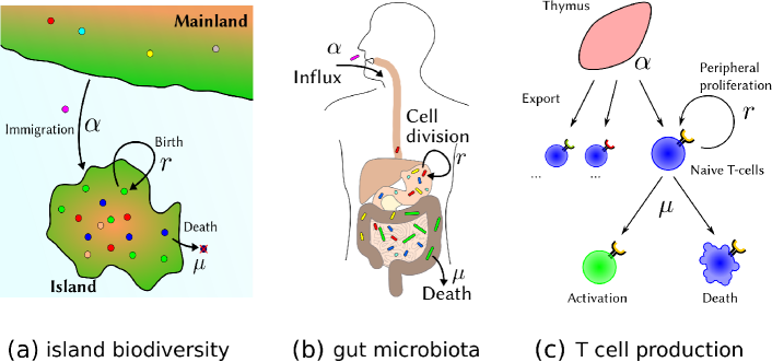
Figure 1: Examples of complex, multicomponent populations in which diversity may be a meaningful quantitative concept. (a) Diversity in island ecology. A large number of species may migrate onto an island. Organisms can proliferate and die, leading to a specific time-dependent pattern of species diversity on the island. (b) Microbes are ingested and form a community in the gut by proliferating, competing, and dying. They can also be cleared from the gut. (c) Naive T cell generation in vertebrates. Naive T cells develop in the thymus. Each T cell expresses only one type of T cell receptor (TCR). Naive T cells can proliferate and die in the peripheral blood. The possible number of T cell receptors that can be expressed is enormous $>10^{15}$, but only perhaps $10^{6}-10^{8}$ different TCRs usually exist in an organism. The diversity of the T cell receptor repertoire is an important determinant of the organism’s response to antigens.

1 Introduction

Diversity is a frequently used concept across a broad spectrum of scientific disciplines, ranging from biology [1, 2, 3, 4, 5] and ecology [6, 7, 8, 9, 10, 11], to investment and portfolio theory [12, 13, 14, 15, 16], to linguistics [17, 18] and sociology [19, 20, 21, 22, 23, 24]. In each of these disciplines, diversity is a measure of the range and distribution of certain features within a given population. It is considered a key attribute that can be dynamically varying, influenced by intra-population interactions, and modified by environmental factors. The concept of diversity, variety, or heterogeneity can be applied to any population. The evolution of the population can also be highly correlated with its diversity. Some examples of biological population dynamics occurring at different scales are shown in Fig. 1. At first sight, diversity seems to be an intuitively simple concept, but since certain population attributes require a full distribution function to quantify, it can be rather complex and difficult to capture using a single metric [25, 3, 4, 26]. We could for example think of a community with a total of four species, with one of the species dominating the total population. Consider a second community that consists of two equally common species. Which one of the two communities exhibits a higher diversity? The first one, because it harbors a larger number of species? Or the second one, because a sample is more likely to contain two species? This example shows that diversity is intrinsically linked to the total number of extant species (richness) and how the population is distributed throughout the species (evenness), and thus cannot be captured by a single number [3]. As a result, there are numerous different diversity indices and associated concepts used in different applications [27, 28, 25, 3, 4, 26, 29]. Nonetheless, diversity measures are important for assessing the current condition of ecosystems, quantifying the influence of environmental factors on different species, and planning conservation efforts [2, 9, 30, 5, 31, 10, 29]. In addition, the concept of diversity is important for the quantitative description of wealth distributions and, more generally, for identifying mechanisms leading to variations in societies [32, 33, 34, 35, 36]. In a broader sense, diversity indices may be helpful for the design of robust energy distribution systems [37] or even to assemble well-performing teams [23]. Thus we see that, despite the ambiguity in the definition of diversity, the concept is very relevant to many different disciplines and applications.

In this topical review, we start by summarizing the basic concepts from information theory which are necessary for a quantitative treatment of diversity. We continue with describing aspects of populations and diversity that are common to many applications in biology. In the next section, we present the common mathematical descriptions of diversity in terms of both number and species counts. Moreover, in most applications, only a small sample of a population is available. Thus, we place particular emphasis on the effects of sampling on diversity measures in Section 5. In Section 6 and subsections within, we survey a number of biological systems in which concepts of diversity play a key role in understanding the dynamics of the population. These include ecological populations, stem cell barcoding experiments, immunology, cancer, and societal wealth distributions. Each of these systems carry their unique attributes and thus require specific diversity measures. Finally, in Section 7 we summarize the advantages and disadvantages of some common diversity measures and conclude with a discussion of possible future applications of concepts of diversity.

2 Entropy, relative entropy, KL divergence, KS statistic, mutual information and all that

We first provide a summary of the fundamental mathematical structures that arise in the analysis of populations in which one naturally seeks to quantitatively compare distributions or frequencies of subpopulations. These mathematical notions invariably involve ideas from information theory such as entropy and mutual information which have a rich history and deep connections to thermodynamics, coding theory, cryptography, inference, and communication [38]. To review the necessary information-theoretic concepts, we consider a discrete random variable $X$ which takes on values from the set $\{x_{1},x_{2},\dots,x_{N}\}$ with probability $P_{k}=\mathrm{Pr}\left(X=x_{k}\right)$ such that

$$\sum_{k=1}^{N}P_{k}=1,$$ (1)

where the sum is taken over all possible values $x_{k}$. This probability mass function may represent the relative frequency that an attribute $X$ takes on the value $x_{k}$ within a large population. In the case of species diversity, we may interpret $P_{k}$ as the relative frequency of species $k$ or the fraction of species with trait $X=x_{k}$ (see clone counts in Section 4).

The entropy, or ‘Shannon entropy,’ is defined by

$$H(X)=-\sum_{k=1}^{N}P_{k}\log P_{k}.$$ (2)

and can be thought of as the expected uncertainty or surprise $-\mathds{E}[\log P(X)]$.

The continuous limit of Shannon entropy, or differential Shannon entropy, has also been defined, but care must be taken if $X$ carries physical dimensions. If the probability of $X$ taking on values in the interval $[x,x+\mbox{d}x]$ is denoted by $P(x)\,\mbox{d}x$, the differential Shannon entropy is

$$H(X)=-\int P(x)\log P(x)\,\mbox{d}x\,.$$ (3)

These expressions are synonymous with the ‘Shannon index’ of species diversity with some freedom in the choice of the base of the logarithm. Without any constraints on the distributions other than being compactly supported, the form of $P_{k}$ or $P(x)$ that maximizes $H(X)$ is a uniform distribution. With additional constraints there are classes of distributions that maximize the Shannon index. For example, for a fixed mean and variance on an unbounded domain, the Shannon index- or entropy-maximizing distribution is Gaussian. Within Gaussian distributions, the Shannon index increases logarithmically with the variance. In fact, within a specific class of distributions, the Shannon index is larger for flatter distributions [39, 40]. As such, the Shannon index has been used as a measure of diversity [41].

One issue with the differential entropy of Eq. (3) is that $P(x)$ carries dimensions $X^{-1}$, because the cumulative distribution function $P(X\leq x)=\int_{-\infty}^{x}P(x^{\prime})\,\mbox{d}x^{\prime}$ has to be dimensionless. Therefore, the argument of the logarithm in Eq. (3) is not dimensionless as required. To avoid such an issue, one can define a point-density function $P_{0}(x)$ according to [39]

$$\lim_{N\to\infty}{\#{\rm points}\in[a,b]\over N}\equiv\int_{a}^{b}P_{0}(x)\mbox{d}x.$$ (4)

Given that the limit is well-behaved, we can express the difference between two adjacent points $x_{k+1}$ and $x_{k}$ in terms of

$$\lim_{N\to\infty}\left[N(x_{k+1}-x_{k})\right]=P_{0}^{-1}(x_{k}).$$ (5)

We now consider the continuum limit of the discrete Shannon entropy as defined in Eq. (2), and set

$$P_{k}=P(x_{k})(x_{k+1}-x_{k})=P(x_{k})\left[NP_{0}(x_{k})\right]^{-1}.$$ (6)

In this way, it is possible to derive a continuous Shannon entropy

$$\lim_{N\to\infty}H_{N}(X) =-\int P(x)\log\left({P(x)\over NP_{0}(x)}\right)\mbox{d}x-\log(N)$$ (7)

$$=-\int P(x)\log\left({P(x)\over P_{0}(x)}\right)\mbox{d}x$$

that is invariant under parameter changes and whose logarithm depends on the dimensionless quantity $P(x)/P_{0}(x)$. We subtracted $\log(N)$ in Eq. (7) to obtain a finite $H_{N}(X)$.

To characterize the diversity between two communities, we consider two discrete random variables $X$ and $Y$ with the corresponding joint probability mass function $P_{X,Y}(x_{k},y_{\ell})=\mathrm{Pr}(X=x_{k},Y=y_{\ell})$. Given the joint distribution $P_{X,Y}(x_{k},y_{\ell})$, we can compute the marginal distributions $P_{X}(x_{k})=\sum_{\ell}P_{X,Y}(x_{k},y_{\ell})$ and $P_{Y}(y_{\ell})=\sum_{k}P_{X,Y}(x_{k},y_{\ell})$ by summing over the complementary variable. These definitions enable us to define the joint entropy

$$H(X,Y)=-\sum_{k,\ell}P_{X,Y}(x_{k},y_{\ell})\log P_{X,Y}(x_{k},y_{\ell}),$$ (8)

which may be also written as $-\mathds{E}[\log P_{X,Y}]$. Moreover, the conditional entropy

$$H(Y|X) =-\sum_{k,\ell}P_{X,Y}(x_{k},y_{\ell})\log\left({P_{X,Y}(x_{k},y_{\ell})\over P_{X}({x}_{k})}\right)$$

$$=-\sum_{k,\ell}P_{X,Y}(x_{k},y_{\ell})\log P_{Y|X}(y_{\ell}|x_{k})$$ (9)

describes the expected uncertainty in the random variable $Y$ given $X$. It can be also expressed as $-\mathds{E}[\log P_{Y|X}]$ where $P_{Y|X}$ is the conditional probability mass function. From symmetry, Eq. (9) also holds when all $X$ and $Y$ are interchanged. For independent random variables $X$ and $Y$, we find that $H(Y|X)=H(Y)$ and $H(X|Y)=H(X)$.

While the Shannon index is a measure of the absolute entropy of a distribution, the relative entropy or Kullback-Leibler (KL) divergence

$$D_{\mathrm{KL}}(P\|Q) =\sum_{k}P(x_{k})\log\left({P(x_{k})\over Q(x_{k})}\right)$$

$$=\mathds{E}_{P}\left[\log P(x_{k})-\log Q(x_{k})\right],$$ (10)

quantifies the distance between two probability mass functions $P$ and $Q$. In the case of continuous distributions $P(x)$ and $Q(x)$, we obtain $D_{\mathrm{KL}}(P\|Q)=\int P(x)\log(P(x)/Q(x))\,\mbox{d}x$.

The KL divergence is the relative entropy of $P$ with respect to the reference distribution $Q$. Note that the limiting Shannon entropy is simply the KL divergence between the distribution $P(x)$ and the associated invariant measure $P_{0}(x)$. Usually, $P$ is an experimental or observed distribution and $Q$ is a model that represents $P$. Furthermore, the KL divergence is nonnegative and equals zero if and only if $P=Q$ [38]. It is not symmetric, $D_{\mathrm{KL}}(P\|Q)\neq D_{\mathrm{KL}}(Q\|P)$, and is thus not a metric. In addition, a special case of the KL divergence is the ‘mutual information’

$$I(X;Y) =D_{\mathrm{KL}}(P_{X,Y}\|P_{X}P_{Y})$$

$$=\sum_{k,\ell}P_{X,Y}(x_{k},y_{\ell})\log\left({P_{X,Y}(x_{k},y_{\ell})\over P_{X}(x_{k})P_{Y}(y_{\ell})}\right)\!.$$ (11)

Note that $I(X;Y)=I(Y;X)$ is symmetric and quantifies how much knowing one variable reduces the uncertainty in the other. If $X$ and $Y$ are completely independent, $I(X,Y)=0$. According to Eq. (11) and the definitions of joint and conditional entropy in Eqs. (9) and (8), the mutual information can be written in terms of marginal, conditional, and joint entropies [38]:

$$I(X;Y) =H(X)-H(X|Y)=H(Y)-H(Y|X)$$

$$=H(X)+H(Y)-H(X,Y).$$ (12)

A symmetric version of the KL divergence is provided by the Jensen-Shannon divergence [42]

$${\rm JSD}(P\|Q)={1\over 2}D_{\mathrm{KL}}(P\|M)+{1\over 2}D_{\mathrm{KL}}(Q\|M),$$ (13)

where $M=(P+Q)/2$ defines the mean distribution of $P$ and $Q$. These divergences can be extended to include multiple and higher-dimensional distributions. The square-root of the Jensen-Shannon divergence is a distance metric between two distributions.

Another useful distance metric is the Kolmogorov-Smirnov (KS) distance, which is defined as

$$D_{\mathrm{KS}}=\max_{x}|G(x)-F(x)|,$$ (14)

where $F(x)$ is a cumulative reference distribution and $G(x)$ is an empirical distribution function. The distribution $G(x)$ is based on different samples with cumulative distribution function that can be $F(x)$ or another distribution to be tested against $F(x)$. The KS metric is the maximum distance between the two cumulative distributions $F(x)$ and $G(x)$. We outline in Section 6.6 that the KS metric is related to the Hoover index which is used to quantify diversity, or inequity, in wealth or income distributions relative to a uniform distribution.

3 Commonly used measures of diversity

The notions of entropy and information are naturally related to the spread of a distribution $P(x)$, and can be subsumed into a general metric for quantifying diversity. Usually, a population is measured and can be thought of as one realization of an underlying distribution. Consider a realization ${\bf n}=\{n_{1},n_{2},\ldots,n_{R}\}$ describing the number $n_{i}$ of entities of a discrete and distinguishable group/species/type ($1\leq i\leq R$). The total population is $N=\sum_{i=1}^{R}n_{i}$. This given realization constitutes a ‘distribution’ across all possible types. Thus, any realization is completely described by a set of $R$ numbers. Diversity measures are reduced representations of the distribution. An example would be a single parameter which captures the spread of the distribution of realizations $\{n_{i}\}$. This is not different than, for example, defining a Gaussian distribution by its mean and standard deviation. Realizations $\{n_{i}\}$, however, usually are not described by specific functions that can be defined by one or two parameters such as Gaussians. However, many different diversity indices can be unified into a single formula called ‘Hill numbers’ of order $q$ [43, 44, 45]:

$${}^{q}\!D=\left(\sum_{i=1}^{R}f_{i}^{q}\right)^{1/(1-q)},$$ (15)

where $f_{i}\equiv n_{i}/N$ is the relative abundance of types $i$. This general formula represents different classes of ‘diversity indices’ for different values of $q$. It is also useful because one can consistently define an effective proportional abundance

$$f_{\rm eff}\mathrel{\vbox{\hbox{\scriptsize.}\hbox{\scriptsize.}}}=1/^{q}\!D=\left(\sum_{i=1}^{R}f_{i}^{q}\right)^{1/(q-1)}$$ (16)

that corresponds to an average abundance with increasing weighting towards the larger-population species as $q$ increases [46, 45].

Note the similarity of this definition to the standard mathematical $p$-norm

$$||{\bf f}||_{p}\mathrel{\vbox{\hbox{\scriptsize.}\hbox{\scriptsize.}}}=\left(\sum_{i=1}^{R}f_{i}^{p}\right)^{1/p},$$ (17)

except that the exponent is $1/p$ instead of $1/(1-q)$. Another diversity measure is provided by the Renyi index [47]

$${}^{q}\!H=\log{}^{q}\!D={1\over 1-q}\log\left(\sum_{i=1}^{R}f_{i}^{q}\right),$$ (18)

which is a generalization of the Shannon entropy defined in Eq. (2). The order $q$ describes the sensitivity of ${}^{q}\!D$ and ${}^{q}\!H$ to common and rare types [48]. Below, we provide an overview of the most commonly used indices which result from the generalized diversity ${}^{q}\!D$ for different values of $q$:

Richness.—In the limit of $q\to 0^{+}$, the probabilities $f_{i}^{q}$ are equal to unity and ${}^{0}\!D$ is simply the total number of types in the population, or the ‘richness’ $R$. The richness is often used in quantifying the diversity of T cells and species counts in ecology [3] and represents a metric that weights all subpopulations equally.

Shannon index.—For $q=1-\varepsilon$ in the limit $\epsilon\to 0^{+}$, the generalized diversity as defined by Eq. (15) becomes

$${}^{1}\!D =\!\lim_{\varepsilon\to 0^{+}}\left(\sum_{i=1}^{R}f_{i}^{1-\varepsilon}\right)^{1/\varepsilon}\!\!\!\!=\lim_{\varepsilon\to 0^{+}}\left(\sum_{i=1}^{R}f_{i}e^{-\varepsilon\ln f_{i}}\right)^{1/\varepsilon}$$

$$=\lim_{\varepsilon\to 0^{+}}\left(\sum_{i=1}^{R}f_{i}(1-\varepsilon\ln f_{i}+O(\varepsilon^{2}))\right)^{1/\varepsilon}$$

$$=\lim_{\varepsilon\to 0^{+}}\left(1-\varepsilon\sum_{i=1}^{R}f_{i}\ln f_{i}\right)^{1/\varepsilon}$$

$$=\exp\left[-\sum_{i=1}^{R}f_{i}\ln f_{i}\right],$$ (19)

which is the exponential of the Shannon index

$${\rm Sh}\mathrel{\vbox{\hbox{\scriptsize.}\hbox{\scriptsize.}}}=\ln\left(\lim_{q\to 1^{-}}{}^{q}\!D\right)=-\sum_{i=1}^{R}f_{i}\log f_{i}$$ (20)

that parallels the Shannon entropy defined in Eqs. (2) and (9). This index is also sometimes called the Shannon-Wiener index ($H$) and can be defined using any logarithmic base. Usually measured values are ${\rm Sh}\sim{\cal O}(1)$. Qualitatively, $e^{\rm Sh}$ can be thought of as a rule of thumb for the number of effective species in a population.

Evenness.—Evenness is another class of diversity indices often invoked in ecological and sociological studies. One definition (‘Shannon’s equitability’) is based on simply normalizing the Shannon diversity by the maximum Shannon diversity that arises if every species is equally likely [49]:

$$J_{\rm E}\mathrel{\vbox{\hbox{\scriptsize.}\hbox{\scriptsize.}}}={{\rm Sh}\over{\rm Sh}_{\rm max}}={{\rm Sh}\over\ln R}.$$ (21)

Simpson’s index with replacement.— When $q=2$, we find

$${}^{2}\!D=1/\left(\sum_{i=1}^{R}f_{i}^{2}\right).$$ (22)

Simpson’s diversity index is defined as

$$S_{\rm r}=1/{{}^{2}\!D}=\sum_{i=1}^{R}f_{i}^{2}=\sum_{i=1}^{R}\left({n_{i}\over N}\right)^{2},$$ (23)

which carries the interpretation that upon drawing an entity from a given population the same type is selected twice.

Simpson’s index without replacement.—A related index that cannot be directly constructed from ${}^{q}\!D$ is Simpson’s index without replacement:

$$S=\sum_{i=1}^{R}{n_{i}(n_{i}-1)\over N(N-1)}.$$ (24)

Here, when an entity is drawn, it is not replaced before the second entity is drawn. The differences between $S_{\rm r}$ and $S$ are significant only for systems with small numbers of entities $n_{i}$ for all types $i$.

Berger-Parker diversity index.—In the $q\to\infty$ limit, we find

$${}^{\infty}\!D =\lim_{q\to\infty}\left(\sum_{i=1}^{R}f_{i}^{q}\right)^{1/(1-q)}$$ (25)

$$=\lim_{q\to\infty}f_{\rm max}^{-\frac{1}{1-1/q}}\left[\sum_{i=1}^{R}\left(\frac{f_{i}}{f_{\rm max}}\right)^{q}\right]^{1/(1-q)}$$

$$=f_{\rm max}^{-1}$$

where $f_{\rm max}=\max_{i\in\{1,\dots,R\}}(f_{i})$. The Berger-Parker diversity index

$$1/{{}^{\infty}\!D}\mathrel{\vbox{\hbox{\scriptsize.}\hbox{\scriptsize.}}}=f_{\rm max}$$ (26)

is defined as the maximum abundance in the set $\{f_{i}\}$, i.e., the abundance of the most common species. It is equivalent to the optimal solution of an $\infty$-norm of ${\bf f}={\bf n}/N$.

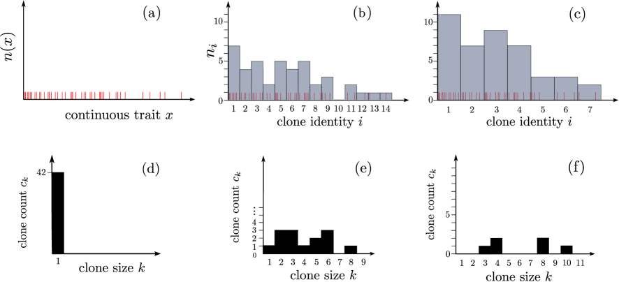
Figure 2: Number counts and clone counts vary depending on the definition and binning of traits or species identity. Both the number counts and clone count distributions can vary significantly as the distinguishability threshold is changed as shown in (a)-(c) and (d)-(f) where the resolution is coarsened.

4 Clone count representation

An alternative way of quantifying a population is through the species abundance distribution or ‘clone counts’ defined by

$$c_{k}\mathrel{\vbox{\hbox{\scriptsize.}\hbox{\scriptsize.}}}=\sum_{i=1}^{R}\mathds{1}(n_{i},k)\in\mathbb{Z}^{+},$$ (27)

where the discrete indicator function $\mathds{1}(n,k)=1$ if $n=k$ and zero otherwise. The sum is usually taken over all species for which $n_{i}\geq 1$. Clone counts can also be defined over only a certain special subset of species. Clone counts, or species abundance distributions in the language of computational mathematics, can be thought of as the measure of the level-sets [50] of the discrete function $n_{i}$, or, in the language of condensed matter physics, the density of states if $n_{i}$ are thought of as energies of states $i$ [51]. The clone counts also satisfy

$$N=\sum_{k=1}^{\infty}kc_{k}\quad\mbox{and}\quad R=\sum_{k=1}^{\infty}c_{k},$$ (28)

where $N$ and $R$ are the discrete total population and the total number of species (richness) present.

Clone counts are commonly used in the theory of nucleation and self-assembly [52, 53, 54], where all particles are identical and $c_{k}$ represents the number of clusters of size $k$. They are equivalent to ‘species abundance distributions’ or sometimes ambiguously described as ‘clone size distributions.’ Clone counts have recently been used to quantify populations in barcoding studies [55] described below.

Clone counts do not depend on the specific labeling of the different types $i$ and do not contain any identity information. However, since the common diversity indices are only a summary of the vector $\{n_{i}\}$ and also do not retain species identity information, ${}^{q}\!D$ can be written in terms of $c_{k}$ rather than $n_{i}$:

$${}^{q}\!D=\left[\sum_{k=1}^{\infty}c_{k}\left({k\over N}\right)^{q}\right]^{1/(1-q)},$$ (29)

which leads to corresponding expressions at specific values of $q$, e.g., ${}^{0}\!D=R$,

$${}^{1}\!D=\exp\left[-\sum_{k=1}^{\infty}c_{k}\left({k\over N}\right)\ln\left({k\over N}\right)\right]\,\,\,\mbox{and}$$

$$1/{{}^{2}\!D}=\sum_{k=1}^{\infty}c_{k}\left({k\over N}\right)^{2}.$$ (30)

While ${}^{q}\!D$ is well-defined when species are discretely delineated, for more granular or continuous traits, the delineation of different species will affect the values of $n_{i}$ and $c_{k}$. Fig. 2 shows population counts ordered by a continuous trait $x$. By defining the discrete species $i$ according to different binning windows over $x$, we find different sets of number and clone counts. Thus, measures of diversity can be highly dependent on the resolution and definition of traits and species.

5 Sampling

In most applications, including all the ones we will discuss below, the entire population is not accessible for identification and measurement. In an ecosystem, all animals of the population cannot be tracked. In blood samples, only a small fraction of the cell types in the whole organism are drawn for identification/sequencing. Thus, inferring the diversity in the entire system from the diversity in the sample is a key problem encountered across many fields.

There are numerous ways to randomly sample a population. One approach is to draw one individual, record its attributes, return it to the system, and allow it to well-mix or equilibrate before again randomly drawing the next individual. This process can be repeated $M$ times. To indicate this type of sampling, we use the subscript $1\times M$ in the corresponding distributions and expectation values. Similar sampling approaches are used in the ‘mark-release-recapture’ experiments to estimate population size [56], survival, and dispersal of mosquitos [57]. For a given configuration $\{n_{i}\}$ and total population size $N$ [58], the probability that the configuration $\{m_{i}\}$ is drawn after $M$ samples is simply

$$P_{\rm 1\times M}({\bf m}|{\bf n},M,N)={M\choose m_{1},m_{2},\ldots,m_{R}}\prod_{j=1}^{R}f_{j}^{m_{j}},$$ (31)

where $f_{j}\equiv n_{j}/N$ is the relative population of species $i$, $N\equiv\sum_{i=1}^{R}n_{i}$ is the total population and $M\equiv\sum_{i=1}^{R}m_{i}$ is the total number of samples.

We can now use $P_{\rm 1\times M}$ to compute the statistics of how the system diversity is reflected in the diversity in the samples. For example, the mean population in the sample in terms of $n_{i}$ is $\mathds{E}_{1\times M}[m_{i}]\equiv\sum_{{\bf m}}{\bf m}P_{\rm 1\times M}({\bf m}|{\bf n},M,N)$. The lowest moments of the populations in the sample are

$$\mathds{E}_{1\times M}[m_{i}]=Mf_{i}=n_{i}{M\over N},$$ (32)

$$\mathds{E}_{1\times M}[m_{i}m_{j}]=f_{i}f_{j}M(M-1)+f_{i}M\mathds{1}(i,j).$$

An alternative random sampling protocol is to draw a fraction $\sigma\equiv M/N<1$ of the entire population once. This type of sampling arises in biopsies such as laboratory blood tests. To be able to distinguish between this sampling protocol and the previous one, we now use the notation $M\times 1$. In this case, the combinatorial probability of a specific sample configuration, given ${\bf n}$, $N$, and $M$ is

$$P_{\rm M\times 1}({\bf m}|{\bf n},M,N)=\prod_{j=1}^{R}\frac{{n_{j}\choose m_{j}}}{{N\choose M}}\mathds{1}\!\left(\!M,\sum_{i=1}^{R}m_{i}\!\right),$$ (33)

where the discrete indicator function enforces the constraint between $m_{i}$ and the sampled population $M$. In this single-draw sampling scenario, we use the Fourier decomposition $\mathds{1}(x,y)\equiv\int_{0}^{2\pi}{\textrm{d}q\over 2\pi}e^{iq(x-y)}$ to find

$$\mathds{E}_{M\times 1}[m_{i}]=n_{i}{M\over N}=n_{i}\sigma,$$ (34)

$$\mathds{E}_{M\times 1}[m_{i}m_{j}]=n_{i}n_{j}{M\over N}{M-1\over N-1}$$

$$\hskip 79.6678pt+\mathds{1}(i,j)n_{i}{M\over N}\left({N-M\over N-1}\right).$$ (35)

Results using $P_{\rm 1\times M}$ and $P_{\rm M\times 1}$ rely on perfectly random sampling, where certain clones/species are not more likely sampled or captured than others. The moments $\mathds{E}[m_{i}m_{j}]$ can be directly used to evaluate the expected Simpson’s diversities, $S_{\rm r}$ (with replacement) and $S$ (without replacement) defined by Eqs. (23) and (24), in the corresponding sample. In the case of $1\times$M sampling, we find

$$\mathds{E}_{\rm 1\times M}[S_{\rm r}] =\mathds{E}_{\rm 1\times M}\left[\sum_{i}\left({m_{i}\over M}\right)^{2}\right]$$

$$={M(M-1)\over M^{2}}\sum_{i}f_{i}^{2}+{1\over M}\sum_{i}f_{i}$$

$$=S_{\rm r}\left(1-{1\over M}\right)+{1\over M},$$ (36)

and

$$\mathds{E}_{\rm 1\times M}[S] =\mathds{E}_{\rm 1\times M}\left[\sum_{i}{m_{i}\over M}{m_{i}-1\over M-1}\right]$$

$$=\sum_{i}{\mathds{E}_{\rm 1\times M}[m_{i}^{2}]\over M(M-1)}-\sum_{i}{\mathds{E}_{\rm 1\times M}[m_{i}]\over M(M-1)}$$

$$=\sum_{i}f_{i}^{2}\equiv S$$ (37)

while for M$\times 1$ sampling, we find

$$\mathds{E}_{\rm M\times 1}[S_{\rm r}] =\mathds{E}_{\rm M\times 1}\left[\sum_{i}\left({m_{i}\over M}\right)^{2}\right]$$

$$=S_{\rm r}{M-1\over M-\sigma}+{1-\sigma\over M-\sigma}$$ (38)

and

$$\mathds{E}_{\rm M\times 1}[S] =\mathds{E}_{\rm M\times 1}\left[\sum_{i}{m_{i}\over M}{m_{i}-1\over M-1}\right]$$

$$=\left[\sum_{i}{\mathds{E}_{\rm M\times 1}[m_{i}^{2}]\over M(M-1)}-\sum_{i}{\mathds{E}_{\rm M\times 1}[m_{i}]\over M(M-1)}\right]$$

$$=S.$$ (39)

Note that for both types of random sampling, we find that the expected Simpson’s diversity (without replacement) in the samples are equal to the Simpson’s diversity in the full system. In general, the expectations do not commute and $\mathds{E}[S]\neq S(\mathds{E}[m_{i}])$.

Effects of sampling on clone counts $c_{k}$ can be similarly calculated by averaging the definition for the sampled clone count

$$b_{k}\mathrel{\vbox{\hbox{\scriptsize.}\hbox{\scriptsize.}}}=\sum_{i=1}\mathds{1}(m_{i},k)\in\mathbb{Z}^{+}$$ (40)

over the sampling probabilities $P_{\rm M\times 1}({\bf m}|{\bf n},M,N)$ or $P_{\rm 1\times M}({\bf m}|{\bf n},M,N)$. For clone counts, the calculations of moments of sampled quantities $b_{k}$ are more involved and explicitly noncommutative $\mathds{E}[b_{k}]\neq\sum_{i}\mathds{1}(\mathds{E}[m_{i}],k)$. One advantage of working in the $b_{k}$ representation is that diversity indices, such as the expected sampled richness $R^{\rm s}$, are difficult to extract from $\mathds{E}[m_{i}]$ but are simply found via $\mathds{E}[R^{\rm s}]=\sum_{k}\mathds{E}[b_{k}]$. Some related results are given in [59, 60].

The above results provide expected diversities in the sample assuming full knowledge of $\{n_{i}\}$ in the system. They represent solutions to the forward problem, the so-called ‘rarefaction’ in ecology. However, the problem of interest is usually the inverse problem, or extrapolation in ecology. In the simplest case, we wish to infer the expected diversity (or $\{n_{i}\}$ and $c_{k}$) in the system from a given configuration $\{m_{i}\}$ or clone count $b_{k}$. Extrapolation is a much harder problem and is the subject of many research papers [61, 62, 63, 64, 65].

One may wish to use the observed sample diversity ${}^{q}\!D(M)$ to approximate the population diversity ${}^{q}\!D(N)$. For any $q$, the underestimation of ${}^{q}\!D(N)$ using ${}^{q}\!D(M)$ decreases as the sample size $M$ increases. The deviation of ${}^{q}\!D(M)$ from ${}^{q}\!D(N)$ is smaller for larger $q$, as higher-order Hill numbers are more heavily weighted by large species, which are less sensitive to subsampling.

Chao and others have shown that for $q\geq 1$ and in the $N\to\infty$ limit, nearly unbiased approximations can be obtained, and when $q\geq 2$, these unbiased estimates are very insensitive to sample size $M$ [59, 60]. Using clone counts in a sample of population $M$, Chao et al. [66] obtained for $q=1$ (in terms of Shannon’s index):

$$\hat{{\rm Sh}}=\sum_{k=1}^{M-1}\frac{1}{k}\!\sum_{1\leq m_{i}\leq M-k}\!\frac{m_{i}}{M}\frac{{{M-m_{i}}\choose{k}}}{{{M-1}\choose{k}}}$$

$$~{}~{}\hskip 5.69054pt-\frac{d_{1}}{M(1-A)^{M-1}}\left\{\log A+\sum_{r=1}^{M-1}\frac{1}{r}(1-A)^{r}\right\},$$ (41)

where $A={2d_{2}}/{[(M-1)d_{1}+2d_{2}]}$.

For $q\geq 2$, Gotelli and Chao [59] obtained

$${}^{q}\!\hat{D}=\left[\sum_{m_{i}\geq q}\frac{m_{i}^{(q)}}{M^{(q)}}\right]^{1/(1-q)}$$ (42)

where $x^{(j)}=x(x-1)...(x-j+1)$. For example, ${}^{2}\!\hat{D}=M(M-1)/\sum_{m_{i}\geq 2}m_{i}(m_{i}-1)$, the inverse of Simpson’s index without replacement (Eqs. 22 and 24).

The ill-conditioning of the inverse problems is particularly severe for the richness ${}^{0}\!D$. The general formula for an estimate of the system richness is

$${}^{0}\!\hat{D}=R(M)+\hat{d}_{0},$$ (43)

and reduces to the unseen species problem for determining $d_{0}$ [67, 68]. Since the sample size $M$ and the richness $R$ in the system are uncorrelated, one must use information contained in the species fractions $f_{i}$ or the clone counts $c_{k}$ in the full system [69, 70]. However, a popular estimate for the system richness $R(N)$ is the ‘Chao1’ estimator [71, 59]

$${\rm Chao1}:\,\hat{R}(N)=R(M)+\frac{d_{1}^{2}}{2d_{2}},$$ (44)

which is actually a lower bound and gives reliable estimates for systems of size only up to approximately double or triple the sample size $M$. The uncertainty of the Chao1 estimator has also been derived via a variance that is also a function of $d_{1}$ and $d_{2}$ [72]. The ‘Chao2’ estimator gives the system richness as a function of measured incidence [59]

$${\rm Chao2}:\,\hat{R}(N)=R(M)+\frac{q_{1}^{2}}{2q_{2}},$$ (45)

where $q_{1},q_{2}$ are the number of species found in 1 or 2 samples out of many (as in the $1\times M$ sampling method). Shen et al. [73] derived another estimate

$$\hat{R}(N)=R(M)+d_{0}\left[1-\left(1-\frac{d_{1}}{Md_{0}+d_{1}}\right)^{\!N-M}\right],$$ (46)

which is only reliable if the sample size $M$ is more than half of the system size $N$. Many of these estimators have been coded into analysis software such as R and iNEXT [74].

Regardless of the estimator, the major limitation is an insufficient sample size $M\ll N$. Models predicting species abundances as a function of system size can help bridge this gap. For example, as log-normal relationship for the clone count $c_{k}$ [75] has been used to find agreeable results [76, 77]. In general, models can be extremely useful for quantifying the effects of sampling, particularly when a Bayesian prior is desired.

We have outlined the basic mathematical frameworks for quantifying diversity that have utility across applications in different disciplines. The above summary of sampling assumes a well-mixed population, precluding any spatial dependence of the distribution of individual species. Spatially dependent sampling has been proposed for the origin of relationships between the number of species detected and the total area occupied by the population (see below).

6 Fields in which diversity play a key role

Below, we summarize a few modern applications in which diversity is important. By no means exhaustive, the following are simply examples of specific systems in biology that reflect the authors’ intellectual biases.

6.1 Ecology, paradox of the plankton

The classic problem in the context of biological diversity is dubbed the paradox of the plankton and was originally discussed in a paper of the same title [78]. It describes diverse populations of plankton in environments with limited resources or nutrients. Sampled populations of plankton exhibit a large number of species even in low nutrient conditions during which one expects strong competition for resources. This observation runs counter to the competitive exclusion principle arising in many settings [79].

Perhaps the most common application of diversity arises in biological population studies, specifically in ecology [6, 7, 8, 9, 10, 11]. Possible areas of application include the monitoring of ecosystems and the development of efficient species conservation strategies [2, 9, 30, 5, 31, 10, 29]. Multiple overlapping and nebulous definitions of ecological diversity have been advanced [27, 28, 25, 3, 4, 26, 29]. Early work by Fisher [6] introduced a logarithmic series model to mathematically describe empirical species diversity data. Here, the diversity index referred to a free parameter in the corresponding model. In a later study, MacArthur defined species diversity based on the size of the sampled area [80]. In the ecological setting, multiple layers of subpopulations are an important feature of populations. These subpopulations may be delineated by another property of the individual species, such as size, weight, behavioral attributes, etc. Subpopulations can also be distinguished through their spatial distribution or occupation of different habitats. Whittaker [81, 82] qualitatively defined four types of diversity (point, alpha, beta, and gamma) conditioned on habitat or spatial distribution of the subpopulations [82]. Fundamentally, these differences arise from different methods of sampling, leading to different Hill numbers ${}^{q}\!D$. We summarize a few often-used descriptions below:

• ‘Point diversity’ refers to samples taken at a single point or ‘microhabitat.’ This quantity is usually operationally measured by trapping organisms at one or more specific points.

• ‘Alpha diversity’ is defined as the diversity within an individual location or specific area. In general, one can define a Hill number derived from measurements at a specific location as ${}^{q}\!D_{\alpha}$, while the index $\alpha\equiv{{}^{0}\!D_{\alpha}}$ is the richness encountered within a defined area or specific location. A few subtle variations in the definition of the index $\alpha$ exist, mostly related to the sampling process [45, 46]. For example, in relation to beta diversity (discussed below), alpha diversity is the mean of the specific-location diversities across all locations within a larger landscape.

• ‘Gamma diversity’ is the diversity index ${}^{q}\!D_{\gamma}$ determined from the entire dataset, the total landscape, or the entire ecosystem. The index $\gamma\equiv{{}^{q}\!D_{\gamma}}$ usually denotes the total number of different species or clones at the largest scale. Note that the mean or sum of the alpha diversities is in most cases not equal to the gamma diversity. The nonlinearity of the Hill numbers as well as the intersection or exclusion of species amongst the different sites suggests a need for indices that connect alpha and gamma diversities.

• ‘Beta diversity’ was devised to describe the difference in diversity between two habitats or between two different levels of ecosystems. While the different levels of diversity are designed to the spatial aspects of diversity, different habitats overlap, leading to some amount of arbitrariness in determining the $\beta$-diversity. Moreover, beta diversity was initially described in different ways [81, 82, 45], leading to confusion about its mathematical definition and use [48, 46, 45]. One possible definition is Whittaker’s [81] multiplicative law ${{}^{q}\!D_{\gamma}}\equiv{{}^{q}\!D_{\alpha}}{{}^{q}\!D_{\beta}}$ where here, $\alpha$ is defined as the mean of the diversities across all micro-habitats. Whittaker’s definition describes beta diversity ${{}^{q}\!D_{\beta}}={{}^{q}\!D_{\gamma}}/{{}^{q}\!D_{\alpha}}$ as a measure to quantify the diversity in the total population relative to the mean diversity across all micro-habitats [45]. In the limit of $q\rightarrow 1^{-}$, we obtain the Shannon diversity relationship ${\rm Sh}_{\gamma}={\rm Sh}_{\alpha}+{\rm Sh}_{\beta}$ according to Eq. (20). Another definition of $\beta$ is given by Lande’s [83] additive law $\gamma\equiv\alpha+\beta$ according to which diversity indices are measured in the same units. One concept associated with $\beta$ in terms of the additive partitioning is ‘species turnover,’ quantifying the difference in richness between the entire and the local population. As an example, consider two distinguishable or spatially separate habitats A and B. If A contains species $\{a,b,c,d,e\}$ and B contains $\{b,c,f,g\}$, we find $\beta_{\texttt{A},\texttt{B}}=5$ associated with the set $\{a,d,e,f,g\}$. The laws of Whittaker and Lande sparked debates about how to properly define beta diversity, and led to the distinction between multiplicative and additive diversity measures [48, 46, 45].

• ‘Delta, Epsilon, Omega diversity’ are other hierarchical definitions of diversities proposed by Whittaker [82]. Delta diversity is analogous to beta diversity but defined at the larger among-landscape scale, while epsilon diversity corresponds to gamma diversity, but at the regional scale that contains many landscapes. Omega diversity is measured at the biosphere scale, and thus characterizes the diversity of all ecosystems [84].

• ‘Zeta diversity’ was introduced by Hui and McGeoch [85], and is defined by a set of $\zeta$ indices that mathematically describe the species numbers between different partitions of a certain habitat. Specifically, $\zeta_{i}$ is the mean number of species shared by $i$ partitions. In particular, $\zeta_{1}$ is the mean richness across all sites. For example, between two samples A and B or sets of data, the average number of species is $\zeta_{1}\mathrel{\vbox{\hbox{\scriptsize.}\hbox{\scriptsize.}}}=(R_{\texttt{A}}+R_{\texttt{B}})/2$, while the intersection is $\zeta_{2}\mathrel{\vbox{\hbox{\scriptsize.}\hbox{\scriptsize.}}}=\texttt{A}\cap\texttt{B}$. Generalizations to multiple samples can be defined using a series of zeta diversity indices $\zeta_{i}$.

• Many other indices have been defined for different applications. The Jaccard index [86, 81, 45, 85] is defined as $J(\texttt{A},\texttt{B})=|\texttt{A}\cap\texttt{B}|/|\texttt{A}\cup\texttt{B}|$, and is a general measure for quantifying the similarity in richness between two sets of populations A and B. Margalef’s index [87] and Menhinick’s index [88] are relative richness measures given by $R/\ln N$ and $R/\sqrt{N}$, respectively. Other indices include the Bray-Curtis dissimilarity [89], the Berger-Parker diversity index [90] as defined in Eq. (26), Fager’s index [91], Keefe and Bergersen’s index [92], McIntosh’s index [93], and Patil and Taillie’s index [94].

A myriad of different definitions of diversity indices arise from specific cases of the Hill numbers and consideration of different spatial scales of ecosystems. There is potential to further unify these definitions in a more systematic way using mathematical norms and more general mathematical structures of spatial dispersal of particles.

6.2 Area-Species Law and Island Biodiversity

A particularly consistent, albeit qualitative feature observed in ecology is the species-area relationship (SAR) which relates the measured number of species (richness) to the relevant area. These areas can represent distinct habitats, such as mountain tops, or islands. For the latter, much work has been done in the subfield of island biodiversity.

The SAR is usually expressed as a power-law relationship between the number of species (or richness) $R$ and the habitat/island area:

$$R=cA^{z},$$ (47)

where $c$ is a constant prefactor and $z$ is an exponent. On a log-log plot, $\log R=\log c+z\log A$ defines a line with slope $z$. An example of the area-species law for species counts of long-horned beetles in the Florida Keys is shown in Fig. 3, yielding a slope $z=0.29$. An alternative species-area relationship is $e^{R}=cA^{z}$ [95], which is a straight line on a semi-log plot.

The classic book by MacArthur and Wilson [96] and many subsequent analyses have promoted and extensively analyzed the SAR idea. In MacArthur and Wilson’s neutral equilibrium theory, immigration to and death on an island are monotonically decreasing and increasing functions of the number of species already on the island, respectively.

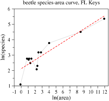
Figure 3: Plot of $\ln R$ versus $\ln A$ with area $A$ measured in terms of km². Species counts of long-horned beetles in the Florida Keys are plotted against the island size [97]. The linear regression line yields a slope of $z=0.29$. Usually, fits of the species-area exponent $z$ yield a small number.

Usually, measured values of the exponent fall in the range $z\sim 0.1-0.4$. Field work has also found relationships between the parameters $c$ and $z$ and system-specific attributes such as the island distance to the mainland, habitat type, etc [96, 98]. Nonetheless, reasonable predictions based on Eq. (47) are ubiquitous across many ecological examples.

Mechanistic origins of the robustness of the SAR have been proposed [99, 100, 101]. Different models for species populations $n_{i}$ or clone counts $c_{k}$ were surveyed, and the corresponding species-area laws were derived by He and Legendre [100]. Spatial clustering of species and the averaging of random measurements were shown to robustly generate a power-law species-area curve [100, 101], highlighting the fundamental importance of sampling.

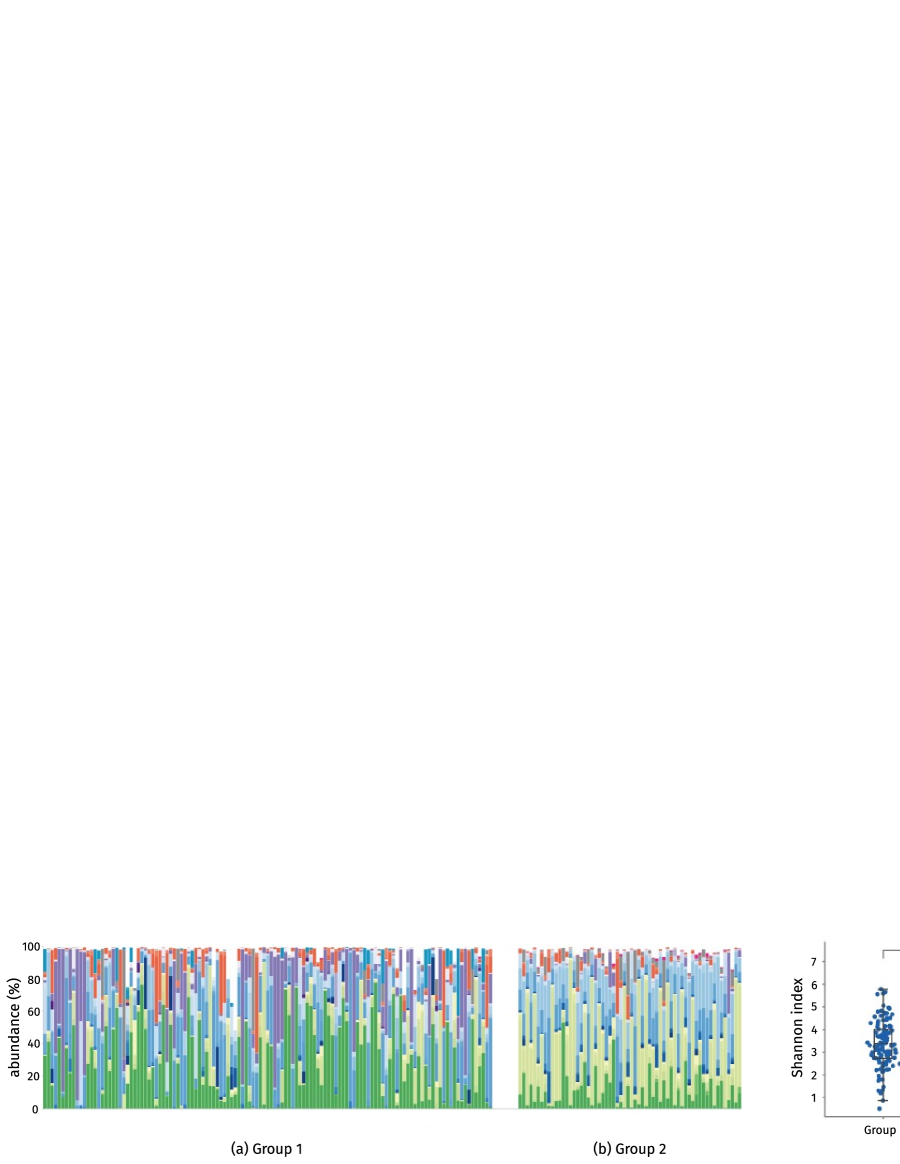
Figure 4: Frequencies of approximately 200 species of bacteria distributed across about a dozen phyla. (a) Group 1 depicts the relative species abundance distribution in samples from patients with Crohn’s disease while (b) Group 2 shows the species pattern in normal patients. The differences in abundance patterns are apparent and have been quantified using the Shannon index for each individual plotted in (c). From Park et al. [102].

6.3 Gut Microbiome

Another ecological system that has recently received much attention is the human microbiome, especially in the gut. The gut bacterial ecosystem is important for health and can impact cardiovascular disease, diabetes, neuropsychiatric diseases, inflammatory bowel disease (IBD), and digestive and metabolic function to the point that fecal transplantation (bacteriotherapy) has become an effective treatment for recurrent C. difficile colitis infections [103]. This type of infection often occurs after antibiotics disrupt the gut microbiome. Transplants have also shown to be effective in treating slow-transit constipation [104].

Recent efforts to collect and curate gut microbiome data have included NIH’s Human Microbiome Project (HMP) [105, 106] and the European Metagenomics of the Human Intestinal Tract (MetaHIT) [107, 108, 109], as well as the integration of the data in [110]. Each dataset contains sequence data from samples from different body regions of hundreds of individuals, both healthy and diseased.

Bacterial species are usually determined by sequencing of the 16S ribosomal RNA (rRNA), a component of prokaryotic ribosomes that contain hypervariable regions that are species-specific. However, closely related taxa can have very similar sequences, making separation imperfect [111]. Nonetheless, with numerous public databases [112, 113, 114, 102], estimates of species abundances in samples are readily available. In the gut, there are usually on the order of $10^{3}$ bacterial species, with Bacteroidetes and Firmicutes being the dominant phyla [115, 116]. Indeed, lower gut diversity is seen to be associated with conditions such as Crohn’s disease [115]. For example, the frequency distribution of bacterial species from healthy and Crohn’s disease patients are shown in Fig. 4. The quantification of diversity of human microbiome is an essential step in ongoing research, and diversity indices have been applied to microbiome data, including $\alpha$-diversity and $\beta$-diversity across the microbiome from different anatomical regions and different patients. As with island biodiversity, the gut microbiome can be modeled as a birth-death-immigration (BDI) process.

6.4 Barcoding Experiments

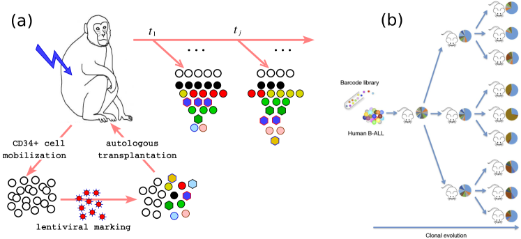
Figure 5: (a) Protocol for Viral Integration Site (VIS) barcode studies of hematopoiesis in rhesus macaque [117, 118, 55]. Here, ‘barcodes’ are defined by the random integration sites of a lentiviral vector. (b) Xenograft barcode experiments using mice [119] in which a library of barcodes was used to tag leukemia-propagating cells before direct transplantation into mice.

Besides taxonomy of gut bacteria, the accurate identification of animal and plant species from samples is an essential task in ecology. In the early 2000’s, a DNA barcoding method was developed to read relatively short DNA regions specific to certain species [120, 121]. These barcodes are usually found in mitochondrial DNA and often derived from a region in the cytochrome oxidase gene [120]. By sequencing samples and comparing them with a sequence database such as The Barcode of Life Data System [122, 123], one can infer the number of species present within a sample. Detecting specific species within samples using DNA barcoding and DNA libraries arises in many applications including identification of birds [121] and flowering plants [124], detection of contaminants [125], and the tracking of plant composition in processed foodstuffs [126].

Recently, a number of barcoding or tagging protocols [127, 128, 129] have been developed to genetically label a large population of cells to study how they differentiate and proliferate, especially in the context of hematopoiesis [130, 117, 118, 131] and cancer progression [132, 133, 134].

A novel approach used to investigate hematopoiesis exploits in situ barcodes [130]. Mice were engineered with an enzyme (Sleeping Beauty Transposase) that randomly moves DNA sequences (transposons) to different parts of the genome. The transposase is designed to be controllable by doxycycline, an antibiotic that can be used to switch on or off gene regulation. When the transposase is briefly activated, transposons within cell genomes are randomly rearranged within a brief period of time. Since the genome length $\gg$ transposon length, the new locations of the transposons will be distinct across the founder cells. After switching off the transposase, proliferation of founder cells imparts the same genomic sequence to their daughter cells. These collections of cells constitute a multiclonal population that proliferates and differentiates.

Analysis of the clonal population within differentiated cell pools shows that granulocytes derive from stem cells at particular time points during the life of the mouse [130]. Comparing clonal abundance structure within different cell lineages shows that clones originally predominant in the lymphoid lineages eventually arise in myeloid cells, indicating that multipotent progenitor cells continually produce cells of both lineages.

In another recent series of studies on hematopoiesis, outlined in Figure 5, stem cells (HSCs) were extracted from rhesus macaques and infected with a lentiviral vector. The lentivirus integrates its genome randomly in the genome of the HSCs. Since the lentivirus genome is much shorter than that of mammalian cells, nearly every successful infection results in a new viral integration site (VIS) or clone. The infected stem cells are autologously transplanted into the animal, and some of them resume differentiation into progenitor cells that transiently proliferate and further differentiate. Descendant cells carry the same genetic sequence, including the lentivirus integration locations, or the viral integration sites (VIS). Another approach is to use libraries of synthesized DNA/RNA as tags. Here, the different sequences, rather than their integration sites, serve as the distinguishing feature. This process avoids the need to determine VISs.

In all of the above approaches, each successive generation of cells will acquire the same tag, VIS or specific DNA barcode sequence as their parent, and ultimately, as the founder HSC. Compared to the Sleeping Beauty Transposon protocol, the VIS or barcoding experiments require an additional viral transfection step. Nonetheless, these VIS and barcoding experiments are equally effective in dissecting the differentiation process and quantifying lineage bias with age. For example, the variation (in time) of the abundances of a clone across different lineages indicates the level of fate switching of a stem cell [117, 135].

These experiments also enabled observation of biological mechanisms on a finer scale compared to traditional studies, allowing inference of parameters that are difficult to measure directly such as the initial HSC differentiation rate and the proliferative potential (number of generations) accessible to progenitor cells [55, 136].

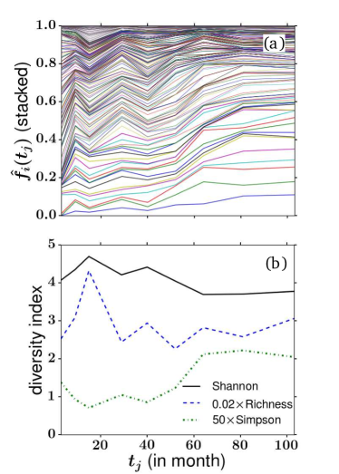
Figure 6: (a) The fractional populations of the largest clones (barcodes) detected in granulocyte blood samples from rhesus macaque. Relative populations are described by the distances between neighboring curves. (b) Diversity indices derived from the data in (a). The Simpson’s index and Shannon diversity are rescaled to fit on the same plot.

After sampling, PCR amplification, and sequencing (each process carrying specific errors), the relative species populations and clone counts within defined cell types can be quantified. Fig. 6(a) shows frequencies of barcode $i$ as a function of sampling times $t_{j}$ in rhesus macaque. The fraction of each clone is depicted by the vertical distance between two neighboring curves. Here, it is important to note that the ‘diversity’ is a measure of the distribution of clone ID (barcodes) instead of lineages (cell types). In Fig. 6(b), we plot three different and rescaled diversity indices associated with the data in (a). The sampled richness is initially low at month 3 when barcoded clones have not fully differentiated and emerged in the peripheral blood. The sampled richness then peaks at month 9 before stabilizing after month 29. Simpson’s diversity seems to continue to increase after month 29, which may indicate more unevenness and coarsening (fewer clones dominating the total population). Shannon’s index is shown to decrease slightly, suggesting a decrease in the effective number of barcodes.

Sun et al. [130] and Kim et al. [117] also used simple clustering algorithms that identified similar clones according to their activity patterns across time. They identified distinct groups of clones that are featured by different time points of contribution to hematopoiesis. Koelle et al. [135] calculated Shannon diversity to ensure comparability across time between animals and different cell types.

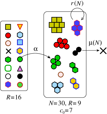
Figure 7: A simple multispecies birth-death-immigration (BDI) process [55, 136, 137, 138]. A constant source (i.e., stem cells with slow dynamics) generated by 16 cells, each of a different clone, undergo asymmetric differentiation with rate $\alpha$ to produce differentiated cells that can undergo birth or death with rates $r(N)$ and $\mu(N)$ that may depend on the total population in the differentiated pool. In this example, the differentiated population contains $N=30$ cells, $R=9$ different clones (barcodes), thus leaving $c_{0}=7$ unseen species.

The employment of neutral barcodes to study blood cell populations is statistically insensitive to spatial partitioning (different tissues in the organism). Nonetheless, small sampling ($M\ll N$) makes inference difficult. Thus, mechanistic simplifications and mathematical models have been used to quantify clonal evolution. Assuming a multispecies birth-death-immigration process (Fig. 7) Dessalles et al. [137] found explicit steady-state distribution functions for $n_{i}$ (log series) and $c_{k}$ (Poisson) for constant $r$ and $\mu$, as well as formulae for the expected Shannon’s and Simpson’s diversities. Goyal et al. [55] derived a master equation for the evolution of $\mathds{E}[c_{k}]$ and then extended the solution to expected clone counts in the progenitor cell and sampled mature cell pools. By comparing results to the expected clone count in the sample at steady-state, they were able to infer kinetic parameters of the differentiation process. Biasco et al. [139] proposed two candidate stochastic models for $n_{i}$ and used Bayesian Information Criterion (BIC) to assess the likelihood of each.

6.5 Cells of the Adaptive Immune System

Another intra-organism system for which diversity is often quantified is the adaptive immune system in vertebrates. The simplest immune subsystem consists of lymphoid cells (e.g., B and T cells) and tissues. B and T cells originate from common lymphoid progenitors (CLPs) that differentiate from HSCs in the bone marrow. B cells develop from CLPs in multiple stages in the bone marrow and spleen, while T cells are formed from CLPs in the thymus. During T cell development in the thymus, T cell receptors (TCRs) are generated by random recombination of the associated receptor gene. TCRs are heterodimeric proteins that usually consist of an alpha chain and a beta chain. After a specific genetic sequence–corresponding to a specific amino acid sequence–is selected, the naive T cell is exported from the thymus into peripheral tissue (such as circulating blood and lymph nodes) where they can further proliferate or interact with antigens presented on the surface of antigen-presenting cells (APCs). Naive T cells (those that have not previously strongly interacted with an antigen) can be activated through association of the surface T cell receptors (TCRs) with antigens presented by major histocompatibility complex (MHC) molecules on the surface of APCs. Similarly, naive B cells are generated in the bone marrow. The B cell receptors (BCRs) are comprised of heavy and light chains and an antigen-binding region, which is generated by the same recombination processes as TCRs. B cells are subsequently activated within tissues by binding to an antigen via their B-cell receptors (BCRs).

The mechanism responsible for creating very diverse repertoires of both BCRs and TCRs is V(D)J recombination [140]. In developing B cells, this mechanism involves the random recombination of diversity (D) and joining (J) gene segments of the heavy chain (DJ recombination). In the following step, a variable (V) gene segment joins the previously formed DJ complex to create a VDJ segment. In light chains, D segments are missing and therefore only VJ segments are generated. During T cell development and TCR generation, gene segments of the alpha chain and beta chain, the VJ and VDJ segments, respectively, also undergo random recombination. In the case of the beta chain, one of two different D regions of thymocytes recombine with one of six different joining J regions first, followed by rearrangement of the variable V region connecting it to the now-combined DJ segment. Due to the missing D segments in alpha chains, only VJ recombination is taking place. The recombination and joining processes in B cells and T cells involve many different genetic deletions and insertions that result in many different BCR and TCR protein sequences and a very large theoretical total number of possible clones with $R\gtrsim 10^{14}-10^{15}$ [141, 142].

In the end, each T or B cell expresses only one TCR or BCR type (an ‘immunotype’ or ‘clonotype’). TCR sequences are preserved during proliferation, while BCR sequences can further evolve [143]. Since the space of antigens (the different amino acid sequences, or epitopes, presented by MHCs) is large, a large number of different TCR and BCR sequences should be present in an organism in order to mount an effective response to a wide range of infections. However, before T cell export from the thymus, a complex selection process occurs [144]. Positive selection eliminates T cells that interact too weakly with MHC molecules. Subsequently, negative selection eliminates those T cells and TCRs that bind too strongly to epitopes. Cells that escape negative selection may lead to autoimmune disease as they react to self-proteins. Thus, the total number of different distinct immunoclones realized in an organism (the richness) defines its T cell repertoire and is estimated to range from $10^{6}-10^{8}$ [145], with the lower range describing mice and the higher range an estimate for humans. B cell richness in man is estimated to be $10^{8}-10^{9}$ [146, 147]. These values are much lower than the theoretical repertoire size $R\gtrsim 10^{14}-10^{15}$. TCR and BCR diversity is an important factor in health. For example, TCR diversity has been shown to influence the tumor microenvironment and lymphoma patient survival [148].

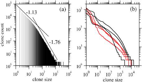
Figure 8: Examples of recently published clone count data. (a) Clone counts derived from a small sample ($10^{5}$ sequences) of T cells [142]. Note the broad distribution described by a biphasic power-law curve. Ignoring the largest clones, power-law fits for each regime yield slopes of -1.13 and -1.76. However, one should be cautious describing sampled TCR (and BCR) clone counts using power laws as they hold typically for far less than two decades. (b) Human TCR clone counts for three HIV-infected (red) and three uninfected (black) individuals show qualitative differences between the distributions (unpublished). Other data from mice and humans, under different conditions and in different cell types, have been recently published [149, 150].

Although specific TCR sequences $i$ can be determined, and their populations $n_{i}$ measured and estimated, the TCR identities vary significantly across individuals (private sequences) so clone counts are usually studied. Fig. 8(a) shows T cell clone counts $b_{k}$ sampled from mice [142] that exhibit a biphasic power-law behavior. Fig. 8(b) shows preliminary clone counts for six individuals, three uninfected patients and three HIV-infected patients [151].

Quantifying T cell diversity is confounded by a number of technical limitations. Usually, the complete T cell repertoire in an animal cannot be directly measured. Rather, as in most other applications, small samples of the entire population are usually drawn. When sampling from animals, the fraction of cells drawn and sequenced is perhaps only $M/N\sim 10^{-5}-10^{-2}$. Thus, clones that have small populations may be missed in the sample. Besides sampling, sequencing requires PCR amplification of the sample, leading to PCR bias, especially in the larger-sized clones [150]. Finally, as in many other applications, there are multiple subclasses of the T cell population. Naive T cells that are activated by antigens develop into memory T cells that carry the same TCR and can further proliferate. Thus, it is difficult to separate the clone counts of different subpopulations such as naive or memory T cells [150].

Many mathematical models for the development and maintenance of the immune systems have been developed [144, 141, 152, 137, 136, 153]. For the multiclonal naive T cell population, rudimentary insights can also be gleaned from a birth-death-immigration process, much as in the modeling of hematopoiesis. Here, the thymus mediates the immigration of a large number of clones, which undergo homeostatic proliferation and death in the periphery. Immigration rates can be different for different clones, depending on the likelihood of specific recombination patterns which may be inferred from probabilistic models of VDJ recombination [154, 155].

Proliferation in the periphery depends on interactions between self-peptides with T cell receptors and is thus clone-dependent. Recently, it has been shown that TCR-dependent thymic output and proliferation rates (a nonneutral BDI model) influence the measured clone count patterns [156]. These processes form and maintain a diverse T cell receptor repertoire, which is usually characterized by its richness. Unlike the barcode abundances arising during hematopoiesis, the neutral BDI processes are not able to capture the shapes of the measured TCR clone counts. It is also known that T cell residence times depend on interactions between tissues and T cell receptors. Thus, different clones of T cells are expected to be differentially spatially distributed in the body. Hence, diversity metrics should be defined within and between habitats, much like that in ecology.

Finally, it is known that T cell richness decreases with age [157, 158, 159, 160]. Qualitatively, a loss of diversity has been predicted within the multispecies BDI process by assuming a decreasing thymic output rate with age. Even when the thymus is abruptly shut down, the diversity of the T cell repertoire slowly decreases as successive clones go extinct and the clone abundance distribution slowly coarsens. In humans, since the overall T cell population is primarily maintained by proliferation rather than thymic immigration [161], the reduction in diversity is fortunately a slow process.

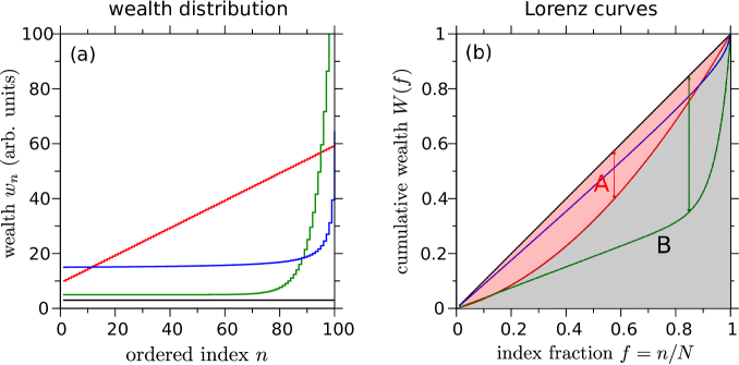
Figure 9: (a) Ordering of all $N=100$ individuals in increasing wealth or income. The hypothetical wealth distributions plotted are $w_{i}=3$ (equal wealth, black curve), $w_{i}=10+(i-1)/2$ (linear distribution, red), $w_{i}=5+e^{i/5-15}-e^{-14.8}$ (green), and $w_{i}=14.5+50/(101-i)$ (blue). The latter three represent distributions with some amount of inequity. (b) These inequalities can be visually quantified by their corresponding Lorenz curves, plotted as the relative fraction of the population $f$. The Lorenz curve for a perfectly uniform wealth distribution is given by the straight diagonal line. The area between the diagonal equality line and any other Lorenz curve can be used to visualize the Gini coefficient of the associated wealth distribution. The Gini coefficient, $\mbox{Gini}=A/(A+B)$, is calculated by dividing the difference in areas between the equality line and the Lorenz curve in question ($A$) by the total area ($A+B=1/2$) under the equality curves. The ‘Robin Hood’ index is defined as the maximum difference between the equality line and a given Lorenz curve, and is indicated by arrow for the red and green Lorenz curves.

6.6 Societal Applications of Diversity: Wealth distributions

Metrics associated with diversity have been naturally applied in human social contexts [21, 19, 20, 162], including physical, cultural, educational [32, 24], and economic settings. For example, the distribution of wealth is the chief metric in many economic and political studies. As with all applications, data collection, sampling, and delineating differences in attributes are main research challenges.

Wealth and income, unlike species, are essentially continuous and ordered quantities, and can be described by many indices designed by economists to measure different wealth attributes of a population. Distinct from cellular or ecological contexts, socio-economic diversity is also often discussed in terms of ‘inequality,’ ‘evenness,’ or ‘polarization.’ Diversity or ‘inequality’ indices in the socioeconomic setting usually invoke a number of additional assumptions:

• Individual identities are irrelevant: This is analogous to barcoding studies of a singular cell type in which the barcode identity is not important.

• Size and total wealth invariance: The diversity is invariant to the total population size. Only proportions of the total population that are associated with a proportion of the total wealth are relevant.

• Dalton principle: Any inequality index should increase if any amount of wealth is transferred from an entity to one with higher existing wealth.

Mathematically, one starts by ordering the wealth or income of a population of $N$ entities $w_{1}\leq w_{2}\ldots\leq w_{i}\leq w_{i+1},\ldots\leq w_{N}$. For large $N$, the rescaled wealth distribution $w(f)\equiv w_{fN}$ is a function of the relative fraction of the total population $f=n/N\in[0,1]$. Furthermore, we can define a normalized wealth distribution or density

$$\tilde{w}(f)={w(f)\over W_{\rm T}},\quad W_{\rm T}=\sum_{i=1}^{N}w_{i}\approx\int_{0}^{1}w(f^{\prime})\mbox{d}f^{\prime},$$ (48)

and the corresponding cumulative distribution

$$W_{i}=\frac{1}{W_{T}}\sum_{j=1}^{i}w_{j}$$ (49)

or

$$W(f)=\int_{0}^{f}\tilde{w}(f^{\prime})\mbox{d}f^{\prime}\equiv\frac{1}{W_{\rm T}}\int_{0}^{f}w(f^{\prime})\mbox{d}f^{\prime}.$$ (50)

The functions $W(f)$ are known as ‘Lorenz-consistent’ if they satisfy the above assumptions [33]. Four representative Lorenz consistent raw wealth distributions are shown in Fig. 9(a) as functions of the individual index. In Fig. 9(b), we plot the continuous cumulative rescaled wealth distribution $W(f)$ as a function of the relative population fraction $f$ corresponding to the wealth distributions shown in Fig. 9(a). From any ordered distribution, we can define a so-called ‘Lorenz curve’ that illustrates many indices graphically. The Lorenz curve is defined as the cumulative wealth of all individuals of a relative index $f=n/N$ and lower.

Many indices can be visualized by the Lorenz curves. For example, the Gini index [163, 164] for the red distribution (linear wealth) in Fig. 9(a) is calculated by the area of the red shaded region ($A$) divided by the area under the equality curve ($A+B=1/2$): $\mbox{Gini}=A/(A+B)=2A$. In a society where every person receives the same income, the Gini index equals zero. However, if the total wealth is concentrated in only one out of $N$ entities, $\mbox{Gini}=1-2/N$. This motivates one to define the Gini index for discrete cumulative wealth values $W_{i}$ according to

$$\mbox{Gini}=1-{2\over N}\sum_{i=1}^{N}W_{i},$$ (51)

while the ‘Hoover’ or ‘Robin Hood’ index defined by [34, 165, 166]

$$H=\max_{f}\left\{|f-W(f)|\right\}$$ (52)

is the Legendre transform at $f^{\ast}$, the fraction of individuals corresponding to $\mbox{d}W(f)/\mbox{d}f|_{f=f^{\ast}}=1$. For the two Lorenz curves in Fig. 9(b), the Robin Hood index is indicated by the two corresponding arrows.

The Robin Hood index happens to be a specific case of the Kolmogorov-Smirnoff statistic as defined in Eq. (14) for two cumulative distributions. For convex functions $W(f)$ that satisfy $W(0)=0$, $W(1)=1$, the index $H$ corresponds to the fraction of the total wealth that needs to be distributed in order to achieve uniform wealth. This can be seen by considering the wealth $w_{i}$ up to an index $n^{\ast}$ such that $w_{i}\leq N^{-1}$ for all $i\leq n^{\ast}$. The total wealth that needs to be redistributed to obtain equal wealth fractions $N^{-1}$ for every individual is

$$H=\sum_{i=1}^{n^{\ast}}\left({1\over N}-w_{i}\right) =\frac{n^{\ast}}{N}-W_{n^{\ast}}$$

$$\approx f^{\ast}-W(f^{\ast}).$$ (53)

Another possibility is to sum over all entities $w_{i}$ according to

$$H ={1\over 2}\sum_{i=1}^{N}\left|{1\over N}-w_{i}\right|$$

$$\approx{1\over 2}\int_{0}^{1}\left|1-w(f)\right|\mbox{d}f$$ (54)

$$=\frac{1}{2}\left[\int_{0}^{f^{\ast}}(1-w(f))\,\mbox{d}f+\int_{f^{\ast}}^{1}(w(f)-1)\,\mbox{d}f\right]$$

$$=f^{\ast}-W(f^{\ast}).$$

The specific, local redistribution is not specified but it would be intriguing to cast it in the language of optimal transport and Wasserstein distances [167]. This way, one might also define costs to wealth redistribution.

It is also possible to quantify inequity according to the Theil index [168, 169, 170]

$$T=\frac{1}{N}\sum_{i=1}^{N}\frac{w_{i}}{\mathds{E}[w]}\log\left(\frac{w_{i}}{\mathds{E}[w]}\right),$$ (55)

which corresponds to a relative entropy as defined in Eq. (10). In this case, the entropy of the distribution of $w_{i}$ is measured with respect to the expected value $\mathds{E}[w]=N^{-1}\sum_{i=1}^{N}w_{i}$. If $\sum_{i=1}^{N}w_{i}=1$, we may interpret $w_{i}$ as the probability of finding an individual in income class $i$, and $\mathds{E}[w]=N^{-1}$ corresponds to the relative share of equally distributed wealth. Naturally, many other measures for inequality have been defined by numerous authors focusing on specific socioeconomic areas [171].

However, typical inequality indices do not convey any judgment, belief system, or behavioral propensity on measured inequity and thus may not capture typical social concepts. In an effort to better quantify concepts such as inequity or ‘polarization,’ [172] a sociologists have proposed a number of polarization indices that are argued to be more directly correlated with social tension and unrest. For example, Esteban and Ray [35, 36] developed a measure of polarization to account for clusters within which individuals are more similar in an attribute $x$ (such as wealth) than they are between clusters. While there may be many ways to define polarization, imposing a few reasonable features and constraints can narrow down the allowable forms. First, they assume an ‘identity-alienation framework’ in which an individual also identifies with his own distribution $f(x)$ at value $x$. An effective ‘antagonism’ of an individual with attribute $x$ towards those with attribute $y$ is defined as $T[f(x),d]$ where a simple form for the distance is $d=|x-y|$. The polarization $P$ is then assumed to take the form

$$P[f]=\int\int T[f(x),|x-y|]f(x)f(y)\,\mbox{d}x\,\mbox{d}y.$$ (56)

By imposing axioms that the polarization (i) cannot increase if the distribution is squeezed (compressed towards its peak), (ii) must increase if two non-overlapping distributions are moved farther apart, and (iii) the polarization should be invariant to scalings of the total population. Using these constraints, the polarization can be more explicitly defined as

$$P[f]=\int\int f^{1+\alpha}(x)f(y)|x-y|\,\mbox{d}x\,\mbox{d}y,$$ (57)

where $1/4\leq\alpha\leq 1$ [36] (Esteban and Ray [35] and Kawada, Nakamura, and Sunada [173] found $0\leq\alpha<1.6$ using slightly different assumptions). The parameter $\alpha$ describes the amount of ‘polarization sensitivity.’ It measures identification of a population with its distribution and distinguishes polarization from other standard inequity measures such as the Gini index (when $\alpha=0$ [35]) or Simpson’s index. Also, note that when $\alpha=0$, the form of $P[f]$ resembles the total potential energy of a system of particles that are distributed according to $f(x)$ and exhibits an interaction energy $|x-y|$. The discrete analogue of Eq. (57) is $P[f]\propto\sum_{i,j}f_{i}^{1+\alpha}f_{j}|x_{i}-x_{j}|$, for which the individuals $i,j$ can be generalized to groups. In empirical studies, the Esteban and Ray polarization measure is given by

$$P_{\rm{ER}}[f]\propto\sum_{i,j}\pi_{i}^{1+\alpha}\pi_{j}|\mu_{i}-\mu_{j}|,$$ (58)

where

$$\pi_{i} =\int_{x_{i-1}}^{x_{i}}\!\!\!f(x)\,\mbox{d}x\quad\rm{and}\quad\mu_{i} =\frac{1}{\pi_{i}}\int_{x_{i-1}}^{x_{i}}\!\!\!xf(x)\,\mbox{d}x,$$ (59)

are the relative frequency and the mean of the wealth in group $i$, respectively [174]. D’Ambrosio and Wolff suggested replacing the difference of mean wealths in Eq. (58) by the Kolmogorov measure of variation distance [174, 175]

$$\mathrm{Kov}_{ij}=\frac{1}{2}\int|f_{i}(y)-f_{j}(y)|\,\mbox{d}y,$$ (60)

to obtain

$$P_{\rm{DW}}[f]\propto\sum_{i,j}\pi_{i}^{1+\alpha}\pi_{j}\rm{Kov}_{ij}.$$ (61)

Additional indices have been proposed, including a class of polarizations by Tsui and Wang [176] of the form

$$P_{\rm TW}({\bf x})={1\over N}\sum_{i=1}^{N}\psi(d_{i}),\quad d_{i}=\bigg{|}{x_{i}-m({\bf x})\over m({\bf x})}\bigg{|},$$ (62)

where $\psi$ is a smooth function of the rescaled distance $d_{i}$. The median income $m({\bf x})$ is computed from the individual incomes $x_{i}$ ($1\leq i\leq N$).

Many of these polarization metrics can in fact be expressed in terms of the Gini coefficient. For example, the Foster–Wolfson polarization index is defined as [177]

$$P_{\rm FW}({\bf x})=({\rm Gini}_{B}-{\rm Gini}_{W})(\mu({\bf x})/m({\bf x})),$$ (63)

where $\mu({\bf x})$ is the corresponding mean income, and the subscript indices $B$ and $W$ denote the between and within group Gini coefficients. According to the definition of $P_{\rm FW}({\bf x})$, inequity differs from polarization in the following way: The Gini index as the sum of ${\rm Gini}_{B}$ and ${\rm Gini}_{W}$ quantifies the unequal distribution of wealth in a society whereas polarization is measured in terms of the difference of ${\rm Gini}_{B}$ and ${\rm Gini}_{W}$. Thus, an increase in within-group inequality leads to a larger total inequality, but a lower polarization. A more refined understanding of socioeconomic diversity will need to consider multiple classes of attributes, including possible geographic or spatial distributions.

The described polarization measures are relevant not only in the context of wealth distributions, but they are also able to provide important insights to other sociological phenomena associated with the notion of diversity. As one example, quantitative measures of polarization are applicable to examine factors that influence the cohesiveness of groups [23]. In this context, the social entropy theory aims to quantitatively compare diversity across social systems such as societies, organizations, and individual groups [19, 178, 20].

7 Summary and Discussion

Table 1: Summary of fundamental, commonly used diversity measures. The variable $q$ indicates the order of the corresponding Hill number ${}^{q}\!D$ as defined in Eq. (15).

Measure Interpretation Application Advantages Disadvantages Species number $n_{i}$ number of entities of type $i$ evolutionary and population models straightforward interpretation in models keeping track of species identity may be unrealistic Species abundance (clone count) $c_{k}$ number of species of size $k$ models of self-assembly/nucleation [52, 53, 54]; characterization of population in barcoding studies [55] directly related to richness, useful when clone identity is not important no clone identity information, insensitive to exchange of populations between clones Richness (${}^{0}\!D$) total number of distinguishable species conservation planning; assessment of ecosystems [3] straightforward mathematical definition and interpretation maximally affected by small sampling; all species are treated equally Evenness (${}^{1}\!D$) uniformity of relative abundances of species in a population characterization of ecosystems and inequity in societies; Theil index [3, 168, 169, 170] straightforward mathematical definition and interpretation; similar to entropy affected by sampling Simpson’s diversity (${}^{2}\!D$) probability that two randomly drawn entities are of the same species characterization of cell populations [147, 179] less affected by sampling more intricate mathematical definition & less interpretability ${}^{q}\!D$, $q>2$ N/A characterization of more frequent species in a population; Berger-Parker index [90] significantly less affected by sampling no intuitive interpretation Lorenz curve cumulative relative wealth economics, wealth distributions fundamental mathematical object no identity information (like ordered clone counts) Gini index deviation of Lorenz curves from absolute equality population-level wealth inequality easily understood no identity information, values are subjectively interpreted Hoover/Robin Hood index KS statistic between Lorenz curve and equality line population-level wealth inequality easily understood no identity information, values are subjectively interpreted

Quantifying the diversity of a given population in terms of a single measure such as richness does not fully describe the underlying distribution of species or other properties. Various diversity measures have been developed and tailored to specific applications in different fields including ecology, biology, and economics. Mathematically, one can describe populations in terms of species numbers $n_{i}$ (number of entities of type $i$) or clone counts $c_{k}$ (number of species of size $k$). Hill numbers ${}^{q}\!D$ provide a framework to unify some common diversity indices that are based on a species-number description. Hill numbers with large values of $q$ put more weight on common species whereas small values of $q$ yield measures that are more sensitive to rarer species. This implies that measures such as richness ($q=0$) and evenness ($q=1$) are more prone to sampling effects than Simpson’s diversity index ($q=2$) or Hill numbers with $q>2$ [180]. In Table 1, we summarize some common diversity measures, their applications, and advantages and disadvantages.

In conclusion, we have provided an overview of the most relevant measures of diversity and their information-theoretic counterparts. We then summarized common applications of diversity indices in biological and ecological systems. Despite the ambiguity in the definitions and the variety of diversity measures [27, 28, 25, 3, 4, 26, 29], the concept is still of great importance for the monitoring of ecosystems and in the context of conservation planning [2, 9, 30, 5, 31, 10, 29].

We also described the importance of a quantitative treatment of diversity for experiments in the study of the gut microbiome, stem cell barcoding, and the adaptive immune system. Finally, we discussed examples of the application of diversity measures in human social systems including the characterization of wealth distributions in societies and measures of political or cultural polarization. Scientific conclusions in these fields and in ecology are particularly sensitive to sampling and measurements. However, accurate measurements [181], meaningful classification, spatial resolution [101], and informative sampling protocols [69, 76] remain elusive across almost all fields. Sometimes, as illustrated in Fig. 6(b), different measures even lead to contradictory conclusions [182]. There is no golden rule in choosing a unique metric for a specific situation, as the sampling effects also depend on the underlying unknown clone-count distribution [180]. It is recommended that one cross-checks different metrics while bearing in mind how sampling effects may impact diversity measures differently.

8 Acknowledgments

This work was supported in part by grants from the NSF through grant DMS-1814364, the Army Research Office through grant W911NF-18-1-0345, and the National Institutes of Health through grant R01HL146552. The authors also thank Greg Huber for insightful discussions.

References

References

- [1] Nei M 1973 Proceedings of the National Academy of Sciences 70 3321–3323
- [2] Heywood V H, Watson R T et al. 1995 Global biodiversity assessment vol 1140 (Cambridge University Press Cambridge)
- [3] Purvis A and Hector A 2000 Nature 405 212
- [4] Whittaker R J, Willis K J and Field R 2001 Journal of Biogeography 28 453–470
- [5] Sala O E, Chapin F S, Armesto J J, Berlow E, Bloomfield J, Dirzo R, Huber-Sanwald E, Huenneke L F, Jackson R B, Kinzig A et al. 2000 Science 287 1770–1774
- [6] Fisher R A, Corbet A S and Williams C B 1943 The Journal of Animal Ecology 42–58
- [7] Magurran A E 1988 Ecological diversity and its measurement (Princeton University Press)
- [8] Benton M J 1995 Science 268 52–58
- [9] Courtillot V and Gaudemer Y 1996 Nature 381 146
- [10] Alroy J 2004 Evolutionary Ecology Research 6 1–32
- [11] Stollmeier F, Geisel T and Nagler J 2014 Physical Review Letters 112 228101
- [12] Blume M E, Crockett J and Friend I 1974 Survey of Current Business 54 16–40
- [13] Blume M E and Friend I 1975 The Journal of Finance 30 585–603
- [14] Rajan R, Servaes H and Zingales L 2000 The Journal of Finance 55 35–80
- [15] Goetzmann W N and Kumar A 2008 Review of Finance 12 433–463
- [16] Haldane A G and May R M 2011 Nature 469 351
- [17] Greenberg J H 1956 Language 32 109–115
- [18] Yule C U 2014 The statistical study of literary vocabulary (Cambridge University Press)
- [19] Bailey K D 1990 Social entropy theory (SUNY Press, Albany, NY)
- [20] Balch T 2000 Autonomous Robots 8 209–238
- [21] Neckerman K M and Torche F 2007 Annu. Rev. Sociol. 33 335–357
- [22] Ostrom E 2009 Understanding Institutional Diversity (Princeton University Press)
- [23] Mäs M, Flache A, Takács K and Jehn K A 2013 Organization Science 24 716–736
- [24] Domina T, Penner A and Penner E 2017 Annual Review of Sociology 43 311–330
- [25] Sepkoski J J 1988 Paleobiology 14 221–234
- [26] Ricotta C 2005 Acta Biotheoretica 53 29–38
- [27] Simpson E H 1949 Nature 163 688
- [28] Hurlbert S H 1971 Ecology 52 577–586
- [29] Sarkar S 2006 Acta Biotheoretica 54 133–140
- [30] John Sepkoski Jr J 1998 Philosophical Transactions of the Royal Society of London. Series B: Biological Sciences 353 315–326
- [31] Margules C R and Pressey R L 2000 Nature 405 243
- [32] Herrnstein R J and Murray C 1994 The Bell Curve (Free Press)
- [33] Lorenz M O 1905 Publications of the American Statistical Association 9 209–219
- [34] Edgar Malone Hoover J 1936 Review of Economics and Statistics 18 162–171
- [35] Esteban J M and Ray D 1994 Econometrica 62 819–851
- [36] Duclos J Y, Esteban J and Ray D 2004 Econometrica 72 1737–1772
- [37] Grubb M, Butler L and Twomey P 2006 Energy Policy 34 4050–4062
- [38] Cover T M and Thomas J A 2012 Elements of information theory (John Wiley & Sons)
- [39] Jaynes E T 1963 Information Theory and Statistical Mechanics Statistical Physics ed Ford K (Benjamin, New York) p 181
- [40] Lazo A and Rathie P 1978 IEEE Transactions on Information Theory 24 120–122
- [41] Spellerberg I F and Fedor P J 2003 Global Ecology and Biogeography 12 177–179
- [42] Lin J 1991 IEEE Transactions on Information theory 37 145–151
- [43] Hill M O 1973 Ecology 54 427–432
- [44] Tuomisto H 2010 Oecologia 164 853–860
- [45] Tuomisto H 2010 Ecography 33 2–22
- [46] Jost L 2007 Ecology 88 2427–2439
- [47] Rényi A et al. 1961 On measures of entropy and information Proceedings of the Fourth Berkeley Symposium on Mathematical Statistics and Probability, Volume 1: Contributions to the Theory of Statistics (The Regents of the University of California)
- [48] Jost L 2006 Oikos 113 363–375
- [49] Heip C 1974 Journal of the Marine Biological Association of the United Kingdom 54 555–557
- [50] Sethian J A 1999 Level Set Methods and Fast Marching Methods: Evolving Interfaces in Computational Geometry, Fluid Mechanics, Computer Vision, and Materials Science (Cambridge University Press)
- [51] Kittel C 1996 Introduction to Solid State Physics, 7th Edition (Wiley)
- [52] Wattis J A D and King J R 1998 Journal of Physics A 31 7169
- [53] D’Orsogna M R, Lakatos G and Chou T 2012 The Journal of Chemical Physics 136 084110
- [54] D’Orsogna M R, Lei Q and Chou T 2015 Journal of Chemical Physics 139 014112
- [55] Goyal S, Kim S, Chen I S Y and Chou T 2015 BMC Biology 13 85
- [56] Villela D A M, Garcia G d A and Maciel-de Freitas R 2017 PLOS Neglected Tropical Diseases 11 1–20
- [57] Epopa P S, Millogo A A, Collins C M, North A, Tripet F, Benedict M Q and Diabate A 2017 Parasites & vectors 10 376
- [58] Cianci D, Broek J V D, Caputo B, Marini F, Torre A D, Heesterbeek H and Hartemink N 2013 Journal of Medical Entomology 50 533–542
- [59] Gotelli N J and Chao A 2013 Measuring and estimating species richness, species diversity, and biotic similarity from sampling data Encyclopedia of Biodiversity vol 5 (Academic Press) pp 195–211
- [60] Chao A, Gotelli N J, Hsieh T, Sander E L, Ma K, Colwell R K and Ellison A M 2014 Ecological Monographs 84 45–67
- [61] Fisher R A, Corbet A S and Williams C B 1943 The Journal of Animal Ecology 12 42–58
- [62] Bunge J and Fitzpatrick M 1993 Journal of the American Statistical Association 88 364–373
- [63] Hsieh T C and Chao A 2016 Systematic Biology 66 100–111
- [64] Cox K D, Black M J, Filip N, Miller M R, Mohns K, Mortimor J, Freitas T R, Greiter Loerzer R, Gerwing T G, Juanes F and Dudas S E 2017 Ecology and Evolution 7 11213–11226
- [65] Budka A, Lacka A and Szoszkiewicz K 2019 Biodiversity and Conservation 28 385–400
- [66] Chao A, Wang Y and Jost L 2013 Methods in Ecology and Evolution 4 1091–1100
- [67] Efron B and Thisted R 1976 Biometrika 63 435–447
- [68] Orlitsky A, Suresh A T and Wu Y 2016 Proceedings of the National Academy of Sciences 113 13283–13288
- [69] Willis A and Bunge J 2015 Biometrics 71 1042–1049
- [70] Willis A 2016 Proceedings of the National Academy of Sciences 113 E5096–E5096
- [71] Chao A 1984 Scandinavian Journal of Statistics 265–270
- [72] Chao A 1987 Biometrics 783–791
- [73] Shen T J, Chao A and Lin C F 2003 Ecology 84 798–804
- [74] Hsieh T C, Ma K H and Chao A 2016 Methods in Ecology and Evolution 7 1451–1456
- [75] Curtis T P, Sloan W T and Scannell J W 2002 Proceedings of the National Academy of Sciences 99 10494–10499
- [76] Locey K J and Lennon J T 2016 Proceedings of the National Academy of Sciences 113 5970–5975
- [77] Locey K J and Lennon J T 2016 Proceedings of the National Academy of Sciences 113 E5097–E5097
- [78] Hutchinson G E 1961 The American Naturalist 95 137–145
- [79] Hardin G 1960 Science 131 1292–1297
- [80] MacArthur R H 1965 Biological Reviews 40 510–533
- [81] Whittaker R H 1960 Ecological Monographs 30 279–338
- [82] Whittaker R H 1977 Evolutionary Biology 10 1–67
- [83] Lande R 1996 Oikos 76 5–13
- [84] Contoli L and Luiselli L 2015 Web Ecology 15 33–37
- [85] Hui C and McGeoch M A 2014 American Naturalist 184 684–694
- [86] Jaccard P 1900 Bull Soc Vaudoise Sci Nat 36 87–130
- [87] Margalef D R 1957 Memorias de la Real Academica de ciencias y artes de Barcelona 32 374–559
- [88] Menhinick E F 1964 Ecology 45 859–861
- [89] Bray J and Curtis J 1957 An ordination of upland forest communities of southern Wisconsin.-ecological Monographs
- [90] Berger W H and Parker F L 1970 Science 168 1345–1347
- [91] Fager E W 1957 Ecology 38 586–595
- [92] Keefe T J and Bergersen E P 1977 Water Research 11 689–691
- [93] McIntosh R P 1967 Ecology 48 392–404
- [94] Patil G and Taillie C 1982 Journal of the American Statistical Association 77 548–561
- [95] Gleason H A 1922 Ecology 3 158–162
- [96] MacArthur R and Wilson E O 1967 The Theory of Island Biogeography (Princeton University Press, Princeton, NJ)
- [97] Browne J and Peck S B 1996 Canadian Journal of Zoology 74 2154–2169
- [98] Volkov I, Banavar J R, Hubbell S P and Maritan A 2003 Nature 424 1035–1037
- [99] Connor E F and McCoy E D 1979 American Naturalist 113 791–833
- [100] He F and Legendre P 2002 Ecology 83 1185–1198
- [101] Martín H G and Goldenfeld N 2006 Proceedings of the National Academy of Sciences 103 10310–10315
- [102] Park S Y, Nanda S, Faraci G, Park Y and Lee H Y 2019 Journal of Biomedical Informatics: X 2 100040
- [103] Wilson B C, Vatanen T, Cutfield W S and O’Sullivan J M 2019 Frontiers in Cellular and Infection Microbiology 9 2
- [104] Tian H, Ge X, Nie Y, Yang L, Ding C, McFarland L V, Zhang X, Chen Q, Gong J and Li N 2017 PLoS ONE 12 e0171308
- [105] Proctor L M, Sechi S, DiGiacomo N D, Fettweis J M, Jefferson K K, III J F S, Rubens C E, Brooks J P, Girerd P P, Huang B, Serrano M G, Sheth N U, Vivadelli S C, Asmussen N C, Borzelleca J F, Bradley S P, Brooks J L, Chalfant C E, Dickinson M R, Drake J I, Edwards D J, Khoury J E, Glascock A L, Gravett M G, Hendricks-Muñoz K D, Koparde V N, Lanni S M, Lara A M, Lee V, Matveyev A V, Ozaki L V, Sexton A S, Shyu C, Tran A, Uetz P H, Wijesinghe D S, Wijesooriya N R, Xu J, Buck G A, Huttenhower C, Gevers D, Sirota-Madi A, Bayer K, Braun J, Denson L A, Jansson J K, Knight R, Kugathasan S, McGovern D P, Petrosino J F, Stappenbeck T S, Birren B W, Clish C B, Gonzalez A, Graeber T G, Lake K, Li X, Loo J, McDonald D, Nicol R, Nusbaum C, Prasad M, Ryu S, Sauk J, Schwager R, Sturgeon H, Tas N, KL K L V, Wilson R G, Yassour M, Xavier R J, Weinstock G, McLaughlin T, Bernstein J A, Zhou W, Piening B D, Kukurba K, Allister C, Butte A J, Boyle S M, Cao L, Chen R, Contrepois K, Craig B C B C, Datta S, Fan-Minogue H, Gu G J, Hanson B, Jiang L, Lek S, Leopold B, Leopold S, Li-Pook-Than J, Mitra S, Rego S, Sailani M R, Salins D, Sodergren E, Pérez P S, Takahashi S, Snyder M P, White O, Mahurkar A and Gwinn-Giglio M 2014 Cell Host & Microbe 16 276–289
- [106] Human Microbiome Project URL https://hmpdacc.org/
- [107] Qin J, Li R, Raes J, Arumugam M, Burgdorf K S, Manichanh C, Nielsen T, Pons N, Levenez F, Yamada T, Mende D R, Li J, Xu J, Li S, Li D, Cao J, Wang B, Liang H, Zheng H, Xie Y, Tap J, Lepage P, Bertalan M, Batto J M, Hansen T, Paslier D L, Linneberg A, Nielsen H B, Pelletier E, Renault P, Sicheritz-Ponten T, Turner K, Zhu H, Yu C, Li S, Jian M, Zhou Y, Li Y, Zhang X, Li S, Qin N, Yang H, Wang J, Brunak S, Doré J, Guarner F, Kristiansen K, Pedersen O, Parkhill J, Weissenbach J, Consortium M, Bork P, Ehrlich S D and Wang J 2010 Nature 464 59–65
- [108] Ehrlich S D and the MetaHIT Consortium 2011 MetaHIT: The European Union Project on Metagenomics of the Human Intestinal Tract Metagenomics of the human body (K. Nelson ed.) (Springer Science+Business Media) chap 15
- [109] MetaHIT Website URL http://www.metahit.eu
- [110] Li J, Jia H, Cai X, Zhong H, Feng Q, Sunagawa S, Arumugam M, Kultima J R, Prifti E, Nielsen T, Juncker A S, Manichanh C, Chen B, Zhang W, Levenez F, Wang J, Xu X, Xiao L, Liang S, Zhang D, Zhang Z, Chen W, Zhao H, Al-Aama J Y, Edris S, Yang H, Wang J, Hansen T, Nielsen H B, Brunak S, Kristiansen K, Guarner F, Pedersen O, Doré J, Ehrlich S D, Consortium M, Bork P and Wang J 2014 Nature Biotechnology 32 834–841
- [111] Vetrovský T and Baldrian P 2013 PLoS ONE 8 e57923
- [112] Metabolomic Workbench URL https://www.metabolomicsworkbench.org/
- [113] Ribosome Database Project URL http://rdp.cme.msu.edu/
- [114] EZBioCloud URL https://www.ezbiocloud.net/
- [115] Shreiner A B, Kao J Y and Young V B 2015 Current Opinion in Gastroenterology 31 69–75
- [116] Thursby E and Juge N 2017 Biochemical Journal 474 1823–1836
- [117] Kim S, Kim N, Presson A P, Metzger M E, Bonifacino A C, Sehl M, Chow S A, Crooks G M, Dunbar C E, An D S, Donahue R E and Chen I S 2014 Cell Stem Cell 14 473–485
- [118] Wu C, Li B, Lu R, Koelle S J, Yang Y, Jares A, Krouse A E, Metzger M, Liang F, Loré K, Wu C O, Donahue R E, Chen I S Y, Weissman I and Dunbar C E 2014 Cell Stem Cell 14 486–499
- [119] Belderbos M E, Koster T, Ausema B, Jacobs S, Sowdagar S, Zwart E, de Bont E, de Haan G and Bystrykh L V 2017 Blood 129 3210–3220
- [120] Hebert P D, Cywinska A, Ball S L and deWaard J R 2003 Proceedings of the Royal Society of London. Series B: Biological Sciences 270 313–321
- [121] Hebert P D N, Stoeckle M Y, Zemlak T S and Francis C M 2004 PLoS Biology 2 e312
- [122] Ratnasingham S and Hebert P D N 2007 Molecular Ecology Notes 7 355–364
- [123] The Barcode of Life Data System URL http://www.barcodinglife.org
- [124] Kress W J, Wurdack K J, Zimmer E A, Weigt L A and Janzen D H 2005 Proceedings of the National Academy of Sciences 102 8369–8374
- [125] Sgamma T, Masiero E, Mali P, Mahat M and Slater A 2018 Frontiers in Plant Science 9 1828
- [126] Bruno A, Sandionigi A, Agostinetto G, Bernabovi L, Frigerio J, Casiraghi M and Labra M 2019 Genes 10 248
- [127] Hawkins J A, Jones S K, Finkelstein I J and Press W H 2018 Proceedings of the National Academy of Sciences 115 E6217–E6226
- [128] Thielecke L, Aranyossy T, Dahl A, Tiwari R, Roeder I, Geiger H, Fehse B, Glauche I and Cornils K 2017 Scientific Reports 7 43249
- [129] Tambe A and Pachter L 2019 BMC Bioinformatics 20 32
- [130] Sun J, Ramos A, Chapman B, Johnnidis J B, Le L, Ho Y J, Klein A, Hofmann O and Camargo F D 2014 Nature 514 322–327
- [131] Perié L and Duffy K R 2016 FEBS letters 590 4068–4083
- [132] Blundell J R and Levy S F 2014 Genomics 104 417 – 430
- [133] Rogers Z N, McFarland C D, Winters I P, Seoane J A, Brady J J, Yoon S, Curtis C, Petrov D A and Winslow M M 2018 Nature Genetics 50 483–486
- [134] Akimov Y, Bulanova D, Abyzova M, Wennerberg K and Aittokallio T 2019 bioRxiv https://doi.org/10.1101/622506
- [135] Koelle S J, Espinoza D A, Wu C, Xu J, Lu R, Li B, Donahue R E and Dunbar C E 2017 Blood 129 1448–1457
- [136] Xu S, Kim S, Chen I S and Chou T 2018 PLoS Computational Biology 14 e1006489
- [137] Dessalles R, D’Orsogna M and Chou T 2018 J. Stat. Phys. 173 182–221
- [138] Xu S 2018 Mathematical Modeling of Clonal Dynamics in Primate Hematopoiesis Ph.D. thesis UCLA
- [139] Biasco L, Pellin D, Scala S, Dionisio F, Basso-Ricci L, Leonardelli L, Scaramuzza S, Baricordi C, Ferrua F, Cicalese M P et al. 2016 Cell Stem Cell 19 107–119
- [140] Alt F W, Oltz E M, Young F, Gorman J, Taccioli G and Chen J 1992 Immunology Today 13 306–314
- [141] Lythe G, Callard R E, Hoare R L and Molina-París C 2016 Journal of Theoretical Biology 389 214–224 ISSN 0022-5193
- [142] Zarnitsyna V, Evavold B, Schoettle L, Blattman J and Antia R 2013 Frontiers in Immunology 4 485
- [143] Hoehn K B, Fowler A, Lunter G and Pybus O G 2016 Molecular Biology and Evolution 33 1147–1157
- [144] Yates A J 2014 Frontiers in Immunology 5 13
- [145] Casrouge A, Beaudoing E, Dalle S, Pannetier C, Kanellopoulos J and Kourilsky P 2000 Journal of Immunology 164 5782–5787
- [146] DeWitt W S, Lindau P, Snyder T M, Sherwood A M, Vignali M, Carlson C S, Greenberg P D, Duerkopp N, Emerson R O and Robins H S 2016 PLoS One 11 e0160853
- [147] Rosenfeld A M, Meng W, Chen D Y, Zhang B, Granot T, Farber D L, Hershberg U and Luning Prak E T 2018 Frontiers in Immunology 9 1472
- [148] Keane C, Gould C, Jones K, Hamm D, Talaulikar D, Ellis J, Vari F, Birch S, Han E, Wood P, Le-Cao K A, Green M R, Crooks P, Jain S, Tobin J, Steptoe R J and Gandhi M K 2017 Clinical Cancer Research 23 1820–1828
- [149] Sethna Z, Elhanati Y, Dudgeon C R, Callan C G, Levine A J, Mora T and Walczak A M 2017 Proceedings of the National Academy of Sciences 114 2253–2258
- [150] Oakes T, Heather J M, Best K, Byng-Maddick R, Husovsky C, Ismail M, Joshi K, Maxwell G, Noursadeghi M, Riddell N, Ruehl T, Turner C T, Uddin I and Chain B 2017 Frontiers in Immunology 8 1267
- [151] Aguilera-Sandoval C R, OYang O, Jojic N, Lovato P, Chen D Y, Boechat M I, Cooper P, Zuo J, Ramirez C, Belzer M, Church J A, and Krogstad P 2017 AIDS 30 701–711
- [152] Lythe G and Molina-París C 2018 Immunological Reviews 285 206–217
- [153] Xu S and Chou T 2018 Journal of Physics A: Mathematical and Theoretical 51 425602
- [154] Marcou Q, Mora T and Walczak A M 2018 Nature Communications 9 561
- [155] Sethna Z, Elhanati Y, Callan Curtis G J, Walczak A M and Mora T 2019 Bioinformatics 35 2974–2981 ISSN 1367-4803
- [156] Dessalles R, D’Orsogna M and Chou T 2019 submitted to: PLoS Computational Biology
- [157] Johnson P, Yates A, Goronzy J and Antia R 2012 Proceedings of The National Academy of Sciences USA 109 21432–21437
- [158] Rane S, Hogan T, Seddon B and Yates A J 2018 PLoS Computational Biology 16 e2003949
- [159] Lewkiewicz S, Chuang Y L and Chou T 2018 Bulletin of Mathematical Biology 81 2783–2817
- [160] Egorov E S, Kasatskaya S A, Zubov V N, Izraelson M, Nakonechnaya T O, Staroverov D B, Angius A, Cucca F, Mamedov I Z, Rosati E, Franke A, Shugay M, Pogorelyy M V, Chudakov D M and Britanova O V 2018 Frontiers in Immunology 9 1618
- [161] den Braber I, Mugwagwa T, Vrisekoop N, Westera L, Mögling R, Bregje de Boer A, Willems N, Schrijver E H R, Spierenburg G, Gaiser K, Mul E, Otto S A, Ruiter A F C, Ackermans M T, Miedema F, Borghans J A M, de Boer R J and Tesselaar K 2012 Immunity 36 288–297
- [162] Maignan C, Ottaviano G, Pinelli D and Rullani F 2003 Fondazione Eni Enrico Mattei
- [163] Gini C 1912 Reprinted in Memorie di metodologica statistica (Ed. Pizetti E, Salvemini, T). Rome: Libreria Eredi Virgilio Veschi
- [164] Gastwirth J L 1972 The Review of Economics and Statistics 54 306–316
- [165] Atkinson A B and Micklewright J 1992 Economic transformation in Eastern Europe and the distribution of income (Cambridge University Press)
- [166] Kennedy B P, Kawachi I and Prothrow-Stith D 1996 British Medical Journal 312 1004–1007
- [167] Galichon A 2017 Optimal Transport Methods in Economics (Princeton University Press)
- [168] Theil H 1972 Statistical decomposition analysis; with applications in the social and administrative sciences Tech. rep.
- [169] Novotnỳ J 2007 The Annals of Regional Science 41 563–580
- [170] Lasarte E, Paniagua M A M et al. 2014 Decomposition of regional income inequality and neighborhood component: A spatial Theil Index Tech. rep. Instituto Valenciano de Investigaciones Económicas, SA (Ivie)
- [171] Maio F G D 2007 Journal of Epidemiology and Community Health 61 849–852
- [172] Böttcher L, Montealegre P, Goles E and Gersbach H 2019 Physica A: Statistical Mechanics and its Applications 123713
- [173] Kawada Y, Nakamura Y and Sunada K 2018 Economics Letters 169 35–27
- [174] D’Ambrosio C and Wolff E N 2006 Is Wealth Becoming More Polarized in the United States? International Perspectives on Household Wealth Chapters (Edward Elgar Publishing) chap 12
- [175] D’Ambrosio C 2001 Review of Income and Wealth 47 43–64
- [176] Wang Y Q and Tsui K Y 2000 Journal of Public Economic Theory 2 349–363
- [177] Wolfson M C 1994 American Economic Review 84 353–358
- [178] Bailey K D 1990 Systems Practice 3 365–382
- [179] Venturi V, Kedzierska K, Turner S J, Doherty P C and Davenport M P 2007 Journal of Immunological Methods 321 182–195
- [180] Soetaertl K and Heip C 1990 Mar. Ecol. Prog. Ser 59 305–307
- [181] Lewis J E, DeGusta D, Meyer M R, Monge J M, Mann A E and Holloway R L 2011 PLoS Biology 9 1–6
- [182] Nagendra H 2002 Applied Geography 22 175–186