Globally optimal registration of noisy point clouds

Abstract

Registration of 3D point clouds is a fundamental task in several applications of robotics and computer vision. While registration methods such as iterative closest point and variants are very popular, they are only locally optimal. There has been some recent work on globally optimal registration, but they perform poorly in the presence of noise in the measurements. In this work we develop a mixed integer programming-based approach for globally optimal registration that explicitly considers uncertainty in its optimization, and hence produces more accurate estimates. Furthermore, from a practical implementation perspective we develop a multi-step optimization that combines fast local methods with our accurate global formulation. Through extensive simulation and real world experiments we demonstrate improved performance over state-of-the-art methods for various level of noise and outliers in the data as well as for partial geometric overlap.

I Introduction

Point cloud registration (PCR) is the problem of finding the transformation that would align point clouds obtained in different frames. This problem is of great importance to the computer vision and robotics community, for instance, estimating pose of objects from lidar measurements [8], performing 3D reconstruction [25], simultaneous localization and mapping [14], robot grasping and manipulation [42], etc. While there exist several methods to perform registration, most notably iterative closest point (ICP) and its variants [3, 30], they are not robust to large initial misalignment, noise and outliers.

Using additional information, such as color/intensity [13], or feature descriptors [11, 31], can help obtain globally optimal registration. But additional information may not be always available (for instance color information is not available when using lidar) and hence we restrict ourselves to applications where only point cloud information is available. Optimizers such as genetic algorithms [33], simulated annealing [19], multiple initial start techniques [35], branch and bound techniques [43], etc. have been used for registration, with weak optimality guarantees [16]. An important reason for the weak guaranty is the lack of explicit optimization over point correspondences.

Recently, Izatt et al. [16] developed a method for global registration using mixed integer programming (MIP). This is a unique approach in that it explicitly reasons about optimal registration parameters as well as correspondence variables. As a result they demonstrate improved results over other global registration approaches especially in the presence of outliers. Their approach to registration uses MIP to minimize a Euclidean distance error between the points . Two major drawbacks of this approach are – (1) lack of robustness to noise, and (2) computationally expensive to scale with increase in number of points.

In this work, we develop a registration approach that can handle noise, outliers and partial data, while ensuring global optimality (see Fig. 1). We improve PCR-MIP-Eu by incorporating sensor and model uncertainty in the optimization, thus making it robust to noise. To the best of our knowledge, this is one of the first works to provide globally optimal solution in the presence of noise uncertainties. Another improvement we offer is a multi-step optimization process to improve computational time, while allowing for registration using greater number of points compared to PCR-MIP-Eu.

By conducting extensive tests on both synthetic and real-world data, we demonstrate superior performance over other global registration methods in terms of accuracy as well as robustness. The remainder of the paper is organized as follows – Section II describes the various related works, Sec. III describes our formulation. The results are presented in Sec. IV, and conclusions are presented in Sec. V.

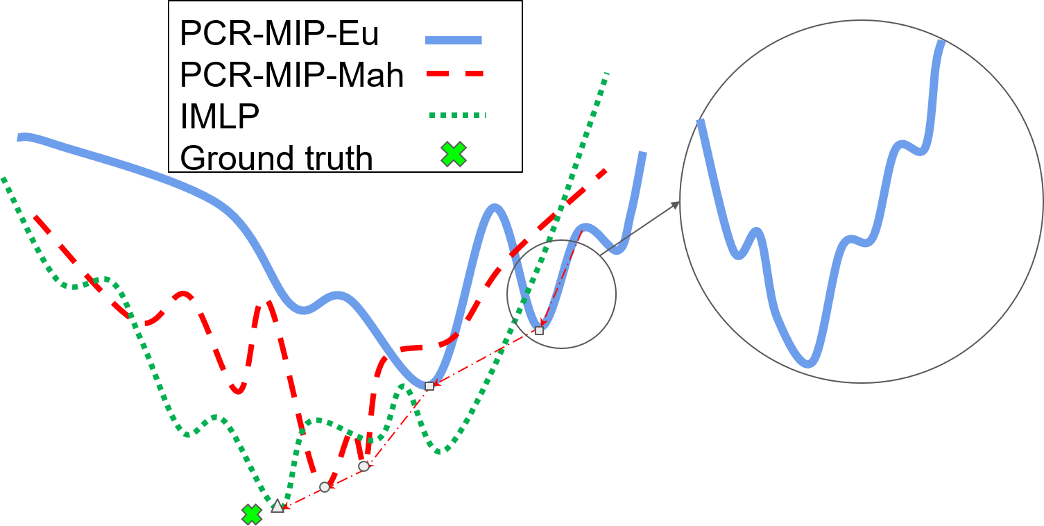
Figure 1: An iconic illustration of optimization functions used for registration by different methods. First we find an approximate pose using PCR-MIP-Eu [16], as shown by the blue curve. Following this, we refine the estimate which reasons for uncertainties using our approach, PCR-MIP-Mah, as shown by the red dashed curve. Finally, we perform a local refinement using IMLP [4] as shown by the green dotted curve. Note than using a multi-step approach allows us to get to a solution very close to the ground truth.

II Related Work

Besl et al. [3] introduced the ICP, which is widely used for registration applications in robotics and computer vision. ICP iteratively estimates the transformation by alternating between, (1) estimating the closest-point correspondences given the current transformation, and (2) estimating the transformation using the current correspondences, until convergence. Several variants of the ICP have been developed (see [30] for a review). Some of the variants incorporate sensor uncertainties [9, 32], are robust to outliers, incorporate uncertainty in finding correspondence [4], are robust to outliers [38, 28], etc. These methods however, need a good initial alignment for convergence.

Using heuristics to find correspondence can improve the robustness of ICP to initial misalignment. However, heuristics are application dependent and what works for one application may not for another. For instance, in probing-based registration for surgical applications, anatomical segments and features can be easily identified by visual inspection. Probing at locations within these anatomical segments can greatly help improve the correspondence as shown in [34, 20]. The works of Gelfand et al. [11] use scale invariant curvature features, Glover et al. [12] use oriented features and Bingham Procrustean alignment, Makadia et al. [21] use extended Gaussian images, Rusu et al. [31] use fast point feature histograms, and Godin et al. [13] use color intensity information for correspondence matching. When dealing with applications where volumetric data is available, curve-skeletons [6] and heat kernel signature [27] can be used to obtain a good initial estimate for the pose.

With the advent for large volumes of easily shareable labeled-datasets, learning-based approaches have gained popularity recently. Learning-based approaches provide good initial pose estimates and rely on local optimizers such an ICP for refined estimates [37, 40, 17, 41]. However, these methods generalize poorly to unseen object instances [2].

In order to widen the basin of convergence, Fitzgibbon et al. [10] developed a Levenberg-Marquardt-based approach. Genetic algorithms and simulated annealing have been used in tandem with ICP to help escape local minima [33, 19]. RANSAC-based hypothesis testing approaches have also been developed, such as the 4PCS [1]. Yang et al. [43] introduced GoICP, a branch and bound-based optimization approach to obtain globally optimal registration. More recently convex relaxation has been used for global pose estimation using Riemannian optimization [29], semi-definite programming [15, 22] and mixed integer programming [16]. A major drawback of the above methods is that none of them consider uncertainty in the points, and are hence not robust to noisy measurements.

TABLE I: Notations

Symbol	Description
$N_{\mathcal{S}}$	number of sensor points
$N_{\mathcal{V}}$	number of model vertices
$N_{\mathcal{M}}$	number of model points
$\boldsymbol{s}_{i}\in\mathbb{R}^{3}$	Sensor point
$\boldsymbol{\Sigma}_{\boldsymbol{s}_{i}}\in\mathbb{R}^{3\times 3}$	Uncertainty associated with $\boldsymbol{s}_{i}$
$\mathcal{V}\in\mathbb{R}^{3\times N_{\mathcal{V}}}$	Set of vertices of a triangular mesh model
$\boldsymbol{C}\in\mathbb{R}^{N_{\mathcal{S}}\times N_{\mathcal{V}}}$	sensor points to model vertices assignment
$\mathcal{M}\in\mathbb{R}^{3\times N_{\mathcal{M}}}$	Points generated on the mesh model
$\boldsymbol{C}^{b}\in\mathbb{R}^{N_{\mathcal{S}}\times N_{\mathcal{M}}}$	sensor points to model points assignment
$\boldsymbol{o}\in\mathbb{R}^{N_{\mathcal{S}}}$	Indicates if a sensor point is an outlier

III Modeling

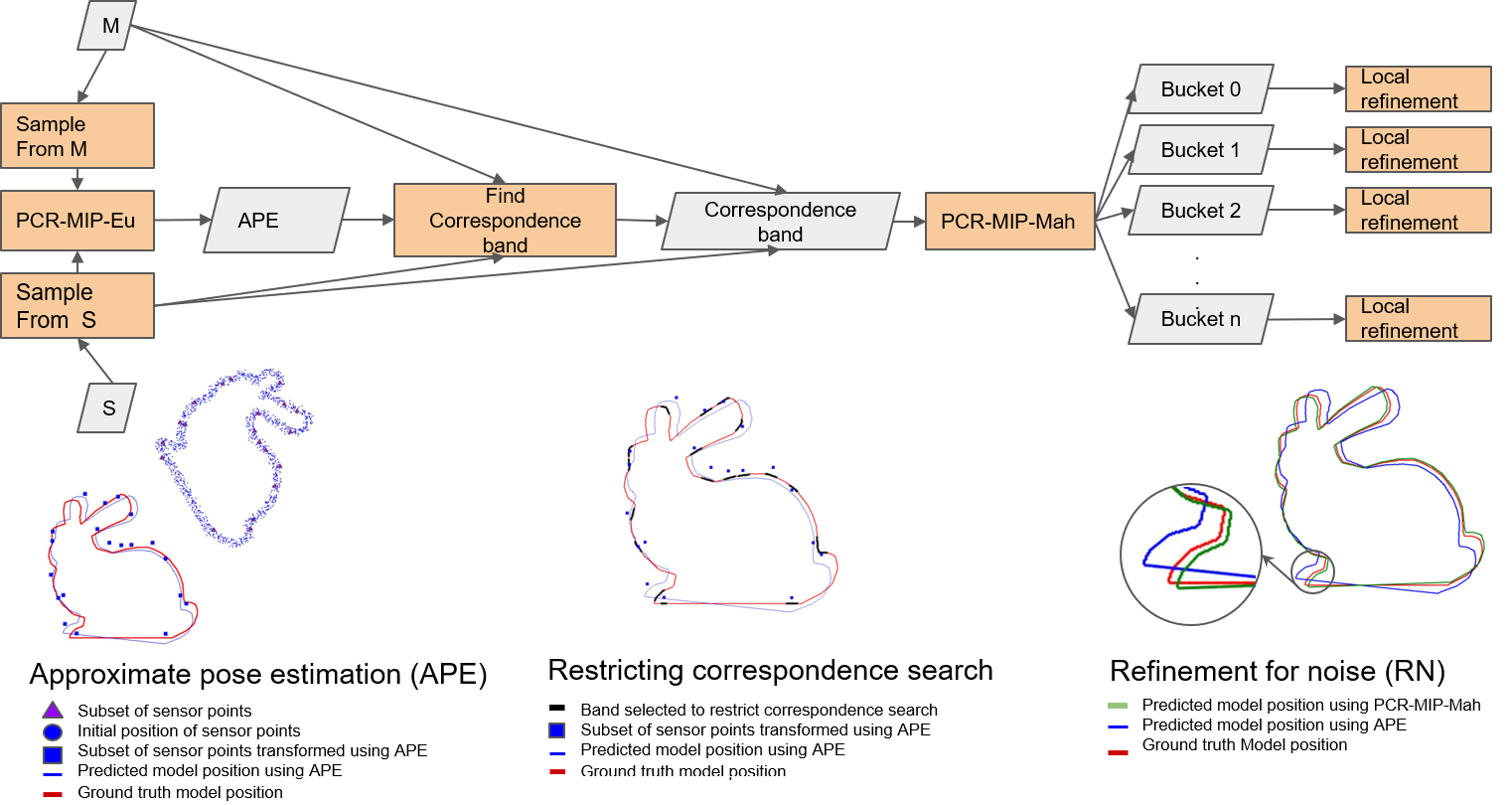
Figure 2: The flowcharts shows various components of the multi-step optimization process that we follow to obtain a globally optimal registration in the presence of uncertainties. There are broadly three steps (1) Approximate pose estimation (APE), (2) Refinement for noise (RN) and (3) Local dense refinement (LDR). We use PCR-MIP-Eu [16] or Go-ICP [43] for APE. We use only a subset of sensor points for APE to get quick and approximate estimates. For RN we use PCR-MIP-Mah which is a mixed integer programming problem that we introduce in this work. Upon finding a refined solution, we further improve it using IMLP [4] for LDR.

Let us consider the problem of registering $N_{s}$ points obtained in the sensor frame to $N_{m}$ points in model frame. We restrict our current analysis to having a uniform isotropic noise represented by $\boldsymbol{C}_{i}^{s}$, $i=1,\dots,N_{s}$ in the sensor points. We however, accommodate anisotropic noise in the model points, and assume they are drawn from a set of normal distributions each having covariance $\boldsymbol{C}_{j}^{m}$, $j=1,\dots,N_{m}$. The uncertainty is lower in the direction of the local surface normal and higher along the tangential plane (refer to [32] for a detailed discussion on this.). Registration is posed as an optimization problem over the pose parameters, $\boldsymbol{R}\in SO(3),\boldsymbol{t}\in\mathbb{R}^{3}$, and correspondence variables $\boldsymbol{H}\in\mathbb{R}^{N_{s}\times N_{m}}$ to minimize the sum of Mahalanobis distance between sensor points and corresponding model points,

$$d_{i,j}^{2} =(\boldsymbol{R}\boldsymbol{s}_{i}+\boldsymbol{t}-\boldsymbol{m}_{j})^{T}\boldsymbol{C}_{ij}^{-1}(\boldsymbol{R}\boldsymbol{s}_{i}+\boldsymbol{t}-\boldsymbol{m}_{j})\quad\text{where},$$ (1)

$$\boldsymbol{C}_{ij} =(\boldsymbol{C}_{j}^{m}+\boldsymbol{R}\boldsymbol{C}_{i}^{s}\boldsymbol{R}^{T}).$$ (2)

The isotropic nature of the sensor noise makes $\boldsymbol{C}_{ij}$ independent of $\boldsymbol{R}$, since $\boldsymbol{R}\boldsymbol{C}_{i}^{s}\boldsymbol{R}^{T}=\boldsymbol{C}_{i}^{s}$ for $\boldsymbol{C}_{i}^{s}=\sigma_{i}\boldsymbol{I}$. We perform Cholesky decomposition on $\boldsymbol{C}_{i,j}^{-1}$ to obtain lower and upper triangular matrix. $\boldsymbol{B}_{i,j}$ and $\boldsymbol{B}_{i,j}^{T}$ respectively, making it convenient to write the Mahalanobis distance in terms of the $l_{1}$ norm,

$$d_{i,j}^{Mah} =\left|\boldsymbol{B}_{i,j}^{T}(\boldsymbol{R}\boldsymbol{s}_{i}+\boldsymbol{t}-\boldsymbol{m}_{j})\right|_{1}.$$ (3)

We prefer the distance in terms of $l_{1}$ norm as opposed to $l_{2}$ norm in order to retain a linear form of the equations. Note that this distance is different from the Euclidean distance used by ICP [3], GoICP [43] and Izatt et al. [16], $d_{i,j}^{Eu}=|\boldsymbol{R}\boldsymbol{s}_{i}+\boldsymbol{t}-\boldsymbol{m}_{j}|_{1}$ .

The objective function to be minimized is obtained from the sum of Mahalanobis distances between all the sensor points and their corresponding model points. We assume that each sensor point can correspond to only one model point (this assumptions may not be true if there are outliers, which we deal with in Sec. III-A), and impose this constraint by introducing a matching matrix $\boldsymbol{H}\in\mathbb{R}^{N_{s}\times N_{m}}$. Each element of this matrix, $\boldsymbol{H}_{i,j}$, is a binary variable that takes value $1$ if $\boldsymbol{s}_{i}$ corresponds to $\boldsymbol{m}_{j}$. We formulate the optimization problem as shown below,

$$\underset{\boldsymbol{R},\boldsymbol{t},\boldsymbol{H}}{minimize} \sum_{i=1}^{N_{s}}\sum_{j=1}^{N_{m}}\left|\boldsymbol{B}_{i,j}^{T}(\boldsymbol{R}\boldsymbol{s}_{i}+\boldsymbol{t}-\boldsymbol{m}_{j})\right|_{1}\boldsymbol{H}_{i,j}$$ (4)

$$\boldsymbol{R}\in SO(3),$$

$$\sum_{j=1}^{N_{m}}\boldsymbol{H}_{i,j}=1.$$

The constraints on $\boldsymbol{R}$ are nonconvex and so we impose piecewise-convex relaxations to it by combining the approaches of [7] and [44]. More details can be obtained from Appendix -A.

The bilinear terms in the objective function (for instance, the term $\boldsymbol{H}_{i,j}\boldsymbol{t}$) poses a challenge to most off-the-shelf MIP optimizers such as Gurobi [26]. In order to deal with this, we introduce additional variables $\beta_{i,j}\in\mathbb{R}^{3}$ and $\phi_{i,j}\in\mathbb{R}$ to ‘convexify’ the problem,

$$\underset{\boldsymbol{R},\boldsymbol{t},\boldsymbol{H}}{minimize} \sum_{i=1}^{N_{s}}\sum_{j=1}^{N_{m}}\phi_{i,j}-(N_{m}-1)\times N_{s}\times\phi_{max1},$$ (5)

subject to

$$\text{Relaxed}\ R\in SO(3),$$

$$\beta_{i,j,k}\geq\pm(\boldsymbol{B}_{i,j}^{T}(\boldsymbol{R}\boldsymbol{s}_{i}+\boldsymbol{t}-\boldsymbol{m}_{j}))_{k},$$ (6)

$$\phi_{i,j},\beta_{i,j,k}\geq 0,$$

$$\phi_{i,j}\geq\sum_{k=1}^{3}\beta_{i,j,k}-(1-\boldsymbol{H}_{i,j})\mathds{M},$$ (7)

$$\phi_{i,j}\geq\phi_{max1}(1-\boldsymbol{H}_{i,j}),$$ (8)

$$\sum_{j=1}^{N_{m}}\boldsymbol{H}_{i,j}=1..$$ (9)

where $\boldsymbol{v}_{k}$ is the $k^{\text{th}}$ component of $\boldsymbol{v}$, $\mathds{M}$ is an arbitrarily large number and $\phi_{max1}$ is a distance threshold for classifying points as outliers . Note that we subtract the term $\phi_{max1}N_{s}(N_{m}-1)$ from $\sum_{ij}\phi_{i,j}$ in the objective function. This is done purely as a convenience of implementation. MIP optimizers often have a termination criteria which is the ratio of the difference between maximum bound and minimum bound of the objective function value to maximum bound of objective function. If we do not subtract the $\phi_{max1}N_{s}(N_{m}-1)$ term, the solver might terminate before reaching the global minimum.

III-A Outlier detection

This formation can be easily extended to detect outliers by modifying Eq. 9 as,

$$\sum_{j=1}^{N_{m}}\boldsymbol{H}_{i,j}+o_{i}=1.$$

$$\phi_{i,j}\geq o_{i}\phi_{max2}$$

$$\phi_{i,j}\geq\sum_{k\in[1,3]}\beta_{i,j,k}-(1-\boldsymbol{H}_{i,j})\mathds{M}-\mathds{M}o_{i},$$

If the distance between sensor point and corresponding model point exceeds the threshold $\phi_{max2}$ then these constraints assign the sensor point as an outlier assigning value $1$ to the variable $o_{i}$.

III-B Restricting correspondence search

In most applications, there is a large number of model points and it may be wasteful to check for correspondences between each pair. Thus we can accelerate the optimization by either using heuristics (as in the case of [44]) or by first finding an approximate correspondence using the method of Izatt et al. [16] or GoICP [43]. We can then restrict the correspondence search to the models points that are close to the approximate correspondence obtained. We assume that we get an approximate range of possible corresponding points is given by $\boldsymbol{Q}\in\mathbb{R}^{N_{s}\times N_{b}}$, where the $i^{\text{th}}$ row of the $\boldsymbol{Q}$ contains indices of $N_{b}$ model points closest to $(\boldsymbol{R}\boldsymbol{s}_{i}+\boldsymbol{t})$. We replace $\boldsymbol{H}$ with $\boldsymbol{H}^{\prime}\in\mathbb{R}^{N_{s}\times N_{b}}$ in Eq. 7-9, and modify Eq. 6 as follows,

$$\beta_{i,j,k}\geq\pm\left(\boldsymbol{B}_{i,\boldsymbol{Q}_{i,j}}^{T}(\boldsymbol{R}\boldsymbol{s}_{i}+\boldsymbol{t}-\boldsymbol{m}_{\boldsymbol{Q}_{i,j}})\right)_{k}$$

III-C Multi-step Optimization

Solving the MIP optimization as described in Eq. 5 is computationally expensive as we increase the total number of sensor points and model points. For example, when we ran PCR-MIP-Mah for 100 sensor points and 100 model points, 64 GB RAM appeared to be insufficient to find the optimal solution. To overcome this problem, we break down the implementation into three parts – (i) Approximate Pose Estimation (APE), Refinement for Noise (RN) and Local Dense Refinement (LDR).

We require four points on a rigid body to uniquely define its 3D pose. This may not be necessarily true for every rigid body especially when the object is symmetric or the points obtained have noise in them. Through empirical observations, Srivatsan et al. [36] have observed that about 20 sensor points are sufficient for most shapes, in order to obtain a reasonable registration estimate. In APE, we randomly select a small subset of sensor points to register with the model points using PCR-MIP-Eu along with ICP to provide heuristics. Since PCR-MIP-Eu optimizes an objective function with Euclidean distance, without accounting for the uncertainty parameters, it has fewer number of optimization variables and quickly provides an approximate pose within a few degrees of misalignment. We use this pose and find an approximate band of $N_{b}$ model points for correspondence calculation for each sensor point.

In RN, we restrict our correspondence search using the solution provided by APE and optimize using PCR-MIP-Mah. Since we are using only a subset of sensor points, it is possible that the solution obtained from PCR-MIP-Mah may not be globally optimal. We select a number of candidate solutions provided by the optimizer ranked by the value of the objective function at those solutions. We then perform a local refinement on all these candidate solutions and select the pose having least objective function value. While performing the LDR we use all the sensor points.

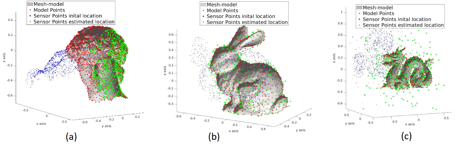
Figure 3: The mesh model is shown in grey, model points are shown in red, initial location of sensor points is shown in blue and estimated locations of registered sensor points is shown in green. (a) Registration with partial overlap for the head of David [18], (b) registration in the presence of noise for Stanford Bunny [39], (c) registration in the presence of outliers for Dragon [39]. In all the three scenarios, our approach finds globally optimal solutions.

IV Results

We implemented our approach on Intel - Core i9-7940X 3.1GHz 14-Core Processor in python 2.7 with Gurobi 7.5.2 for mixed integer branch and bound optimization. While generating synthetic data, for model points, we sampled 1 to 10 points from each face of the mesh model. Around 1000 Sensor points were sampled independent of the model points and an isotropic Gaussian noise was added to each sensor point. These sensor points were then transformed with a random, but known ground truth transformation to check accuracy of the solution given by our method.

TABLE II: Results for varying Correspondence band sizes

	Band size	Rot.	Trans.	TRE	Obj val
		error (deg)	error
Ground truth		0	0	0	449.60
ICP		141.09	1.14	0.49	20564.99
IMLP		112.65	0.944	0.46	2623.41
GoICP		0.33	$2\times 10^{-3}$	$1.2\times 10^{-3}$	408.41
PCR-MIP-Eu		2.93	0.02	0.01	2696.55
PCR-MIP-Mah	5	0.10	$2\times 10^{-4}$	$8.2\times 10^{-5}$	173.72
APE +RN +LDR		0.10	$2\times 10^{-5}$	$1.55\times 10^{-5}$	164.93
PCR-MIP-Mah	20	1.26	0.01	$7\times 10^{-3}$	719.81
APE +RN +LDR		0.10	$2\times 10^{-5}$	$1.5\times 10^{-5}$	164.93
PCR-MIP-Mah	30	1.22	0.01	$7\times 10^{-3}$	720.02
APE +RN +LDR		0.10	$2\times 10^{-5}$	$1.5\times 10^{-5}$	164.93
PCR-MIP-Mah	50	1.28	0.01	$7\times 10^{-3}$	731.66
APE +RN +LDR		0.10	$2\times 10^{-5}$	$1.5\times 10^{-5}$	164.93

IV-A Robustness to varying correspondence bands

We sub-sampled 20 sensor points for the APE using PCR-MIP-Eu. We set the maximum run time for PCR-MIP-Eu to be 300 seconds (though the solver converged to a solution in much less than this time in most cases) which provides pose estimates with a rotation error of approximately $3^{\circ}$ from the ground truth. It is common practice to use heuristics to hasten the search for optimal solutions in MIP implementations [16]. In our implementation, every time the solver found a feasible solution, we used ICP (with approx 300 sensor and 500 model points) as heuristics, and provided the solution back to PCR-MIP-Mah for efficient branch and bound search. In this section, we present results for registration of a partial point cloud to a model of the head of David [18] as shown in Fig. 3(a). We tested our method for band sizes of 5, 20, 30 and 50. Table II shows the error in the rotation (in degrees), error in translation, target registration error (TRE) , and value of the objective function in Eq. 5. These results are compared with ICP, GICP, IMLP, PCR-MIP-Eu and GoICP . As we increase the band size, the chances of PCR-MIP-Mah to get stuck in a local valley are high. But even then, the LDR helps to get closer to the ground truth, when compared to the other methods. It is worth noting that the misalignment for this experiment was very high that ICP and IMLP failed to estimate the registration altogether. The average time taken by ICP is 0.1s, IMLP is 10.2s, GoICP is 1.5min, PCR-MIP-Mah is 5min. The IMLP used in LDR only takes 1.2s on an average. Instead of choosing a band of correspondences of fixed size, one could also restrict the correspondences based on a distance threshold. Note that in Table II, PCR-MIP-Mah can also be interpreted as APE +RN. As illustrated in Fig. 1, it is clear that the multistep process helps produce the most accurate solution to this problem. As interesting observation we make from the last column of Table II is that, the value of the objective function ( see Eq. 5) is lowest for our approach, even lower than the value at the ground truth registration. Infact, the value of objective function is most similar to the ground truth for GoICP. One must be cautious about this observation because, Izatt et al. [16] and Yu and Ju [44] have observed scenarios where GoICP produced poor results compared to PCR-MIP-Eu.

TABLE III: Results for varying noise

	Rot. error (∘)	Trans. error	TRE	Obj val
$\sigma=5\times 10^{-5}$
Ground truth	0	0	0	28394.42
ICP	127.16	1.31	0.56	331829.18
IMLP	129.36	1.25	0.60	1158433.99
GoICP	0.30	$4.2\times 10^{-3}$	$1.8\times 10^{-3}$	28778.12
PCR-MIP-Eu	1.76	0.02	0.012	42562.80
PCR-MIP-Mah	0.23	$1\times 10^{-3}$	$9.9\times 10^{-4}$	28616.78
APE +RN +LDR	0.23	$2.8\times 10^{-3}$	$9.8\times 10^{-4}$	28245.36
$\sigma=10^{-4}$
Ground truth	0	0	0	13988.28
ICP	159.51	0.43	0.41	104004.00
IMLP	143.74	0.37	0.51	370540.86
GoICP	0.32	$2\times 10^{-3}$	$2\times 10^{-3}$	14131.38
PCR-MIP-Eu	3.72	0.02	0.02	30430.84
PCR-MIP-Mah	0.27	$2.2\times 10^{-3}$	$2.3^{-3}$	14592.16
APE +RN +LDR	0.22	$1.5\times 10^{-3}$	$1.5\times 10^{-3}$	13983.39
$\sigma=5\times 10^{-3}$
Ground truth	0	0	0	370.39
ICP	77.35	0.62	0.28	2275.62
IMLP	61.36	0.51	0.24	1981.30
GoICP	0.67	$5\times 10^{-}3$	$4\times 10^{-}3$	385.69
PCR-MIP-Eu	2.94	0.02	0.01	553.57
PCR-MIP-Mah	0.29	$3.5\times 10^{-3}$	$2\times 10^{-3}$	372.78
APE +RN +LDR	0.14	$2\times 10^{-3}$	$1\times 10^{-3}$	368.35
$\sigma=10^{-2}$
Ground truth	0	0	0	240.77
ICP	176.09	0.83	0.62	1229.01
IMLP	172.39	0.84	0.621120.02
GoICP	1.08	$9\times 10^{-3}$	$5.4\times 10^{-3}$	242.56
PCR-MIP-Eu	1.78	0.01	$7\times 10^{-3}$	260.43
PCR-MIP-Mah	1.18	$9\times 10^{-3}$	$6\times 10^{-3}$	241.95
APE +RN +LDR	0.62	$4\times 10^{-3}$	$5\times 10^{-3}$	235.48
$\sigma=4\times 10^{-2}$
Ground truth	0	0	0	166.53
ICP	55.00	0.35	0.31	445.86
IMLP	54.69	0.35	0.30	381.18
GoICP	3.70	0.04	0.02	158.62
PCR-MIP-Eu	5.09	0.04	0.02	170.65
PCR-MIP-Mah	5.30	0.04	0.02	158.97
APE +RN +LDR	2.33	0.02	0.01	157.26

IV-B Robustness to varying levels of noise

We tested our method for noise levels varying from $\sigma=5\times 10^{-5}$ to $4\times 10^{-2}$ in a model restricted to fit in a $1\times 1\times 1$ unit box. We select a band of around 20 model points neighboring the corresponding model point obtained from the APE solution. For this experiment we consider a Stanford bunny [39] (Fig. 3(b) shows the result for $\sigma=10^{-2}$). From Table III, we observe that the accuracy of all the methods decrease as the noise is increased. Among all the methods, PCR-MIP-Mah consistently provides good estimates, which are then refined by LDR taking it closer to the global optima. We also observe that the solution obtained by LDR after APE is not as accurate as APE followed by RN and then LDR. Another point to note is that the average time taken for GoICP was much higher compared to the previous experiments with no noise. GoICP took an average of 15 min to find a solution and sometimes required tuning of tolerance parameters to produce any solution in reasonable time.

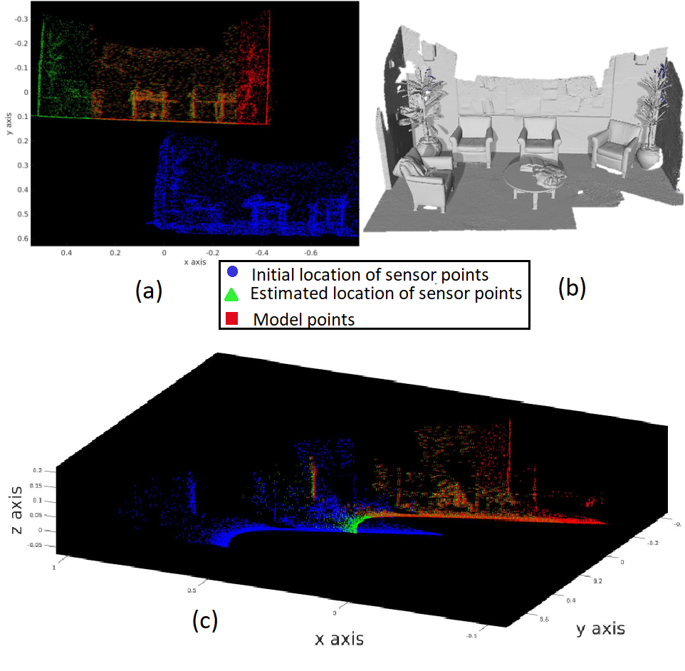
Figure 4: Model points are shown in red, initial location of sensor points is shown in blue and estimated locations of registered sensor points is shown in green. (a) Registration result on realworld RGBD dataset of a lounge. We only use the point cloud locations and neglect the RGB information. Note that the green and red points are noisy and have partial overlap, yet our approach is able to register them accurately. (b) Rendered view of the lounge dataset from [45]. (c) Registration of point clouds obtained from a velodyne lidar from the Oakland dataset [24].

IV-C Robustness to partial overlap and outliers

To check for the robustness of our approach to outliers, we tested it on synthetic data of a dragon [39] as shown in Fig. 3(c). We used a variant of ICP called Trim-ICP [5] to deal with outliers, when used as a heuristic in APE. Keeping the initial misalignment constant, we added different percentages of outliers and tested the robustness of our approach. Table IV shows the errors for various percentage of outlier data. We observe that our approach is robust to presence of outliers, which is critical when used with real world data.

TABLE IV: Results for varying levels of outliers

Outlier ($\%$)	Rot. error (∘)	Trans. error	TRE
10	0.80	$4\times 10^{-3}$	$5\times 10^{-3}$
20	0.95	$5\times 10^{-3}$	$6\times 10^{-3}$
40	0.49	$4\times 10^{-3}$	$3\times 10^{-3}$

We also tested our approach on two real world data sets. The first is an example of 3D reconstruction from RGBD point cloud. For this experiment we considered RGBD scans of a lounge [45] (See Fig. 4 (b) ). We ignored the color information and only used the point cloud information. Fig. 4(a) shows the initial position of point clouds obtained from two different views in red and blue colors. Based on a prior knowledge of the sensor used, we use an approximate sensor uncertainty in the blue points. For the red points, we use PCA analysis similar to the work of Esterpar et al. [9], to find the covariance along local surface normal and the tangential plane. The estimated error in the rotation is $2.09^{\circ}$ and translation is $0.28$cm. The estimated location of the points, shown in green aligns well with the red points, despite presence of only a partial overlap, as shown in Fig. 4(a).

We repeat this analysis for another experiment involving realworld measurement obtained from a Velodyne lidar sensor. We use scans from the Oakland dataset for this experiment [24]. The estimated error in the rotation is $0.38^{\circ}$ and translation is $0.7$cm. Just to show the versatility of our framework, we use GoICP for APE in this example. Once again we observe that our approach registers the red and blue point clouds and produces an accurate alignment as shown by the green points in Fig. 4(c).

V Discussions and Future Work

In this work, we presented a mixed integer programming (MIP) based approach for globally optimal registration, while considering uncertainty in the point measurements. We observe that our approach is effective at finding optimal solutions are various level of noise and outliers as well as effectively deal with partial overlap in the data. Our implementation involves multi-step optimization, which allows for fast computation without compromising on the quality of the final result. We believe that in applications where registration accuracy is of great importance and real-time performance is not critical, our approach can be very effective in providing a benchmark for finding optimal solutions.

The implementation can be made faster by incorporating application specific local heuristic solvers. We demonstrated improved performance using a few popular local approaches, however, our framework is flexible enough to use any other local heuristics methods. As exciting future direction that we are currently pursuing involves using data-driven techniques to provide fast heuristics for the MIP solvers without the requirement for correspondence calculations.

Currently, we use an off-the-shelf MIP optimizer which is a generalized solver and not specifically optimized for our problem. Since we know the structure of our problem, we believe that the branch and bound search strategy could be modified to effectively find solutions for our problem. In the future we plan to relax the isotropic uncertainty assumption in the sensor points and extend the approach to consider anisotropic uncertainty. We also plan to incorporate surface normal and curvature information as well as introduce a regularization term to perform deformable registration.

-A Rotation matrix constraints

Consider the rotation matrix $\boldsymbol{R}=[\textbf{u}_{1},\textbf{u}_{2},\textbf{u}_{3}]^{T}\in SO(3)$, where $\boldsymbol{u}_{i}$ are orthogonal unit vectors. There exist the following constraints on $\boldsymbol{R}$, $\boldsymbol{R}^{T}\boldsymbol{R}=\boldsymbol{I}$ and $\det(\boldsymbol{R})=1$. Since these constraints add nonconvexity to the problem, we approximate the constraint on each element of $\boldsymbol{R}$ with piecewise-convex approximations .

Orthogonality constraints

In order to approximate the orthogonality constraints $\boldsymbol{R}^{T}\boldsymbol{R}=\boldsymbol{I}$, we divide the range $[-1,1]$ in $n$ intervals with $k^{\text{th}}$ interval being $[q_{k},q_{k+1}]$. We introduce auxiliary variables $\textbf{w}\in\mathbb{R}^{3x3}$ and $\lambda^{i,j}\in\mathbb{R}^{n+1}$ such that,

$$\begin{bmatrix}\textbf{u}_{i}(j)\\ \text{{w}}_{i}(j)\\ \end{bmatrix}=\sum_{k=0}^{n}\lambda_{k}^{i,j}\begin{bmatrix}q_{k}\\ q_{k}^{2}\\ \end{bmatrix},\lambda^{i,j}\text{in sos2}$$

$$\textbf{u}_{i}^{T}\textbf{u}_{i}\leq 1$$

$$\text{{w}}_{i}(1)+\text{{w}}_{i}(2)+\text{{w}}_{i}(3)\geq 1,$$

$$|\textbf{u}_{i}\pm\textbf{u}_{j}|_{2}^{2}\leq 2$$

$$|\textbf{u}_{1}\pm\textbf{u}_{2}\pm\textbf{u}_{3}|_{2}^{2}\leq 3.$$

For a discussion on sos2 constraints, refer to [7]. In this work we choose the number of partitions for the sos2 constraints to be 50. Increasing the number of partitions improves the result but also increases the computation time.

Bi-linear terms

In order to impose the constraint $\det(\boldsymbol{R})=1$, which can also be written as $\textbf{u}_{i}\times\textbf{u}_{j}=\textbf{u}_{k}$, we use McCormick constraints [23], This constraint involves bi-linear terms (for e.g. $\mathbf{R}_{3,1}=\mathbf{R}_{1,2}\mathbf{R}_{2,3}+\mathbf{R}_{2,2}\mathbf{R}_{1,3}$) and the non-linearity makes the problem difficult to solve. We apply the relaxation of every such bi-linear term $xy$ where $x$ and $y$ are two continuous variables such that $x\in[x_{lb},x_{ub}]$ and $y\in[y_{lb},y_{ub}]$. For rotation matrix components, these upper bounds and lower bounds are $1$ and $-1$ respectively. We approximate each bi-linear term $xy$ by a new scalar variable $v$. We apply McCormick relaxation and find out over (concave) and under (convex) envelop function for the bi-linear term. This gives $v$ as a close linear approximation of the bi-linear term $xy$.

$$concave(xy) =min(-y+x+1,y-x+1)$$

$$convex(xy) =max(-y-x+1,y+x-1)$$

$$v \geq-y-x-1,$$

$$v \geq y+x-1,$$

$$v \geq y-x+1,$$

$$v \geq-y+x+1,$$

$$convex(xy) \leq v\leq concave(xy).$$

We use the following convention,

$$v_{1} =\boldsymbol{R}_{1,3}\boldsymbol{R}_{2,2},$$

$$v_{2} =\boldsymbol{R}_{1,2}\boldsymbol{R}_{2,3},$$

$$v_{3} =\boldsymbol{R}_{2,1}\boldsymbol{R}_{1,3},$$

$$v_{4} =\boldsymbol{R}_{1,1}\boldsymbol{R}_{2,3},$$

$$v_{5} =\boldsymbol{R}_{2,1}\boldsymbol{R}_{1,2},$$

$$v_{6} =\boldsymbol{R}_{1,1}\boldsymbol{R}_{2,2}.$$

Using these approximations for each bi-linear term, each element of the rotation matrix can be approximated. For example, since $\boldsymbol{R}\in SO(3)$, $\boldsymbol{R}_{3,1}=\boldsymbol{R}_{1,2}\boldsymbol{R}_{2,3}-\boldsymbol{R}_{2,2}\boldsymbol{R}_{1,3}$ (cross product of first and second column equals third column), $\boldsymbol{R}_{3,1}=(v_{2}-v_{1})$. The other elements can be similarly obtained.

References

- Aiger et al. [2008] Dror Aiger, Niloy J Mitra, and Daniel Cohen-Or. 4-points congruent sets for robust pairwise surface registration. In ACM Transactions on Graphics (TOG), volume 27, page 85. ACM, 2008.
- Balntas et al. [2017] Vassileios Balntas, Andreas Doumanoglou, Caner Sahin, Juil Sock, Rigas Kouskouridas, and Tae-Kyun Kim. Pose Guided RGBD Feature Learning for 3D Object Pose Estimation. In Proceedings of the IEEE Conference on Computer Vision and Pattern Recognition, pages 3856–3864, 2017.
- Besl and McKay [1992] P.J. Besl and Neil D. McKay. A method for registration of 3-D shapes. IEEE Transactions on Pattern Analysis and Machine Intelligence, 14(2):239–256, Feb 1992. ISSN 0162-8828. doi: 10.1109/34.121791.
- Billings et al. [2015] Seth D. Billings, Emad M. Boctor, and Russell H. Taylor. Iterative Most-Likely Point Registration (IMLP): A Robust Algorithm for Computing Optimal Shape Alignment. PLoS ONE, 10, 2015.
- Chetverikov et al. [2005] Dmitry Chetverikov, Dmitry Stepanov, and Pavel Krsek. Robust Euclidean alignment of 3D point sets: the trimmed iterative closest point algorithm. Image and Vision Computing, 23(3):299–309, 2005.
- Cornea et al. [2005] Nicu D Cornea, M Fatih Demirci, Deborah Silver, SJ Dickinson, PB Kantor, et al. 3D object retrieval using many-to-many matching of curve skeletons. In Shape Modeling and Applications, 2005 International Conference, pages 366–371. IEEE, 2005.
- Dai et al. [2017] Hongkai Dai, Gregory Izatt, and Russ Tedrake. Global inverse kinematics via mixed-integer convex optimization. In International Symposium on Robotics Research, Puerto Varas, Chile, pages 1–16, 2017.
- Ding et al. [2008] Min Ding, Kristian Lyngbaek, and Avideh Zakhor. Automatic registration of aerial imagery with untextured 3d lidar models. In Computer Vision and Pattern Recognition, 2008. CVPR 2008. IEEE Conference on, pages 1–8. IEEE, 2008.
- Estépar et al. [2004] Raúl San José Estépar, Anders Brun, and Carl-Fredrik Westin. Robust generalized total least squares iterative closest point registration. In International Conference on Medical Image Computing and Computer-Assisted Intervention, pages 234–241. Springer, 2004.
- Fitzgibbon [2003] Andrew W Fitzgibbon. Robust registration of 2D and 3D point sets. Image and Vision Computing, 21(13-14):1145–1153, 2003.
- Gelfand et al. [2005] Natasha Gelfand, Niloy J Mitra, Leonidas J Guibas, and Helmut Pottmann. Robust global registration. In Symposium on geometry processing, volume 2, page 5, 2005.
- Glover et al. [2012] Jared Glover, Gary Bradski, and Radu Bogdan Rusu. Monte carlo pose estimation with quaternion kernels and the distribution. In Robotics: Science and Systems, volume 7, page 97, 2012.
- Guy Godin [1994] Rejean Baribeau Guy Godin, Marc Rioux. Three-dimensional registration using range and intensity information, 1994. URL https://doi.org/10.1117/12.189139.
- Holz and Behnke [2010] Dirk Holz and Sven Behnke. Sancta simplicitas-on the efficiency and achievable results of slam using icp-based incremental registration. In Robotics and Automation (ICRA), 2010 IEEE International Conference on, pages 1380–1387. IEEE, 2010.
- Horowitz et al. [2014] Matanya B Horowitz, Nikolai Matni, and Joel W Burdick. Convex relaxations of SE(2) and SE(3) for visual pose estimation. In IEEE International Conference on Robotics and Automation (ICRA), pages 1148–1154. IEEE, 2014.
- Izatt and Tedrake [2017] Gregory Izatt and Russ Tedrake. Globally Optimal Object Pose Estimation in Point Clouds with Mixed-Integer Programming. In International Symposium on Robotics Reesearch, 2017.
- Kendall et al. [2015] Alex Kendall, Matthew Grimes, and Roberto Cipolla. PoseNet: A convolutional network for real-time 6-DOF camera relocalization. In IEEE International Conference on Computer Vision (ICCV), pages 2938–2946. IEEE, 2015.
- Levoy et al. [2000] Marc Levoy, Kari Pulli, Brian Curless, Szymon Rusinkiewicz, David Koller, Lucas Pereira, Matt Ginzton, Sean Anderson, James Davis, Jeremy Ginsberg, et al. The digital michelangelo project: 3d scanning of large statues. In Proceedings of the 27th annual conference on Computer graphics and interactive techniques, pages 131–144. ACM Press/Addison-Wesley Publishing Co., 2000.
- Luck et al. [2000] Jason Luck, Charles Little, and William Hoff. Registration of range data using a hybrid simulated annealing and iterative closest point algorithm. In Proceedings of IEEE International Conference on Robotics and Automation, pages 3739–3744. IEEE, 2000.
- Ma and Ellis [2003] Burton Ma and Randy E Ellis. Robust registration for computer-integrated orthopedic surgery: laboratory validation and clinical experience. Medical image analysis, 7(3):237–250, 2003.
- Makadia et al. [2006] Ameesh Makadia, Alexander Patterson, and Kostas Daniilidis. Fully automatic registration of 3D point clouds. In Computer Vision and Pattern Recognition, 2006 IEEE Computer Society Conference on, volume 1, pages 1297–1304. IEEE, 2006.
- Maron et al. [2016] Haggai Maron, Nadav Dym, Itay Kezurer, Shahar Kovalsky, and Yaron Lipman. Point registration via efficient convex relaxation. ACM Transactions on Graphics (TOG), 35(4):73, 2016.
- McCormick [1976] Garth P McCormick. Computability of global solutions to factorable nonconvex programs: Part i—convex underestimating problems. Mathematical programming, 10(1):147–175, 1976.
- Munoz et al. [2009] Daniel Munoz, J Andrew Bagnell, Nicolas Vandapel, and Martial Hebert. Contextual classification with functional max-margin markov networks. In Computer Vision and Pattern Recognition, 2009. CVPR 2009. IEEE Conference on, pages 975–982. IEEE, 2009.
- Newcombe et al. [2011] Richard A Newcombe, Shahram Izadi, Otmar Hilliges, David Molyneaux, David Kim, Andrew J Davison, Pushmeet Kohi, Jamie Shotton, Steve Hodges, and Andrew Fitzgibbon. Kinectfusion: Real-time dense surface mapping and tracking. In Mixed and augmented reality (ISMAR), 2011 10th IEEE international symposium on, pages 127–136. IEEE, 2011.
- Optimization [2014] Gurobi Optimization. Inc.,“gurobi optimizer reference manual,” 2015. URL: http://www. gurobi. com, 2014.
- Ovsjanikov et al. [2010] Maks Ovsjanikov, Quentin Mérigot, Facundo Mémoli, and Leonidas Guibas. One point isometric matching with the heat kernel. In Computer Graphics Forum, volume 29, pages 1555–1564. Wiley Online Library, 2010.
- Phillips et al. [2007] Jeff M Phillips, Ran Liu, and Carlo Tomasi. Outlier robust ICP for minimizing fractional RMSD. In 3-D Digital Imaging and Modeling, 2007. 3DIM’07. Sixth International Conference on, pages 427–434. IEEE, 2007.
- Rosen et al. [2016] David M Rosen, Luca Carlone, Afonso S Bandeira, and John J Leonard. A certifiably correct algorithm for synchronization over the special Euclidean group. 12th International Workshop on Agorithmic Foundations of Robotics, 2016.
- Rusinkiewicz and Levoy [2001] Szymon Rusinkiewicz and Marc Levoy. Efficient Variants of the ICP Algorithm. In Third International Conference on 3D Digital Imaging and Modeling (3DIM), June 2001.
- Rusu et al. [2009] Radu Bogdan Rusu, Nico Blodow, and Michael Beetz. Fast point feature histograms (fpfh) for 3d registration. In IEEE International Conference on Robotics and Automation, pages 3212–3217. IEEE, 2009.
- Segal et al. [2009] Aleksandr Segal, Dirk Haehnel, and Sebastian Thrun. Generalized-ICP. In Robotics: Science and Systems, volume 2, 2009.
- Seixas et al. [2008] Flávio Luiz Seixas, Luiz Satoru Ochi, Aura Conci, and Débora Muchaluat Saade. Image registration using genetic algorithms. In Proceedings of the 10th annual conference on Genetic and evolutionary computation, pages 1145–1146. ACM, 2008.
- Simon et al. [1995] David A Simon, Martial Hebert, and Takeo Kanade. Techniques for fast and accurate intrasurgical registration. Journal of image guided surgery, 1(1):17–29, 1995.
- Srivatsan and Choset [2016] Rangaprasad Arun Srivatsan and Howie Choset. Multiple start branch and prune filtering algorithm for nonconvex optimization. In The 12th International Workshop on The Algorithmic Foundations of Robotics. Springer, 2016.
- Srivatsan et al. [2017] Rangaprasad Arun Srivatsan, Prasad Vagdargi, and Howie Choset. Sparse point registration. In 18th International Symposium on Robotics Research, 2017.
- Tang et al. [2013] Danhang Tang, Tsz-Ho Yu, and Tae-Kyun Kim. Real-time articulated hand pose estimation using semi-supervised transductive regression forests. In IEEE International Conference on Computer Vision (ICCV), pages 3224–3231. IEEE, 2013.
- Tsin and Kanade [2004] Yanghai Tsin and Takeo Kanade. A correlation-based approach to robust point set registration. In European conference on computer vision, pages 558–569. Springer, 2004.
- [39] Greg Turk and Marc Levoy. The Stanford 3D Scanning Repository. Stanford University Computer Graphics Laboratory http://graphics.stanford.edu/data/3Dscanrep.
- Vongkulbhisal et al. [2017] Jayakorn Vongkulbhisal, Fernando De la Torre, and Joao P Costeira. Discriminative optimization: theory and applications to point cloud registration. In IEEE CVPR, 2017.
- Xiang et al. [2016] Yu Xiang, Wonhui Kim, Wei Chen, Jingwei Ji, Christopher Choy, Hao Su, Roozbeh Mottaghi, Leonidas Guibas, and Silvio Savarese. Objectnet3D: A large scale database for 3d object recognition. In European Conference on Computer Vision, pages 160–176. Springer, 2016.
- Xiang et al. [2017] Yu Xiang, Tanner Schmidt, Venkatraman Narayanan, and Dieter Fox. Posecnn: A convolutional neural network for 6d object pose estimation in cluttered scenes. arXiv preprint arXiv:1711.00199, 2017.
- Yang et al. [2013] Jiaolong Yang, Hongdong Li, and Yunde Jia. Go-ICP: Solving 3D Registration Efficiently and Globally Optimally. In 2013 IEEE International Conference on Computer Vision (ICCV), pages 1457–1464, Dec 2013. doi: 10.1109/ICCV.2013.184.
- Yu and Ju [2018] Chanki Yu and Da Young Ju. A maximum feasible subsystem for globally optimal 3d point cloud registration. Sensors, 18(2):544, 2018.
- Zhou and Koltun [2013] Qian-Yi Zhou and Vladlen Koltun. Dense scene reconstruction with points of interest. ACM Transactions on Graphics (ToG), 32(4):112, 2013.