Planar semilattices and nearlattices with eighty-three subnearlattices
Abstract.
Finite (upper) nearlattices are essentially the same mathematical entities as finite semilattices, finite commutative idempotent semigroups, finite join-enriched meet semilattices, and chopped lattices. We prove that if an -element nearlattice has at least subnearlattices, then it has a planar Hasse diagram. For , this result is sharp.
Key words and phrases:
Planar nearlattice, planar semilattice, planar lattice, chopped lattice, number of subalgebras, computer-assisted proof, commutative idempotent semigroup1991 Mathematics Subject Classification:
06A12, 06B75, 20M101. Result and introduction
At first, after few definitions, we formulate our main (and only) result; historical and other comments and an outline of the paper will be given thereafter.
Definition 1.1.
Let be a finite -element join-semilattice. Its natural ordering is defined by . For , let be the infimum of provided it exists. If this infimum does not exist, then is undefined. The structure is called a finite (upper) nearlattice; note that this nearlattice and the join-semilattice mutually determine each other. Apart from a short historical survey, the adjective “upper” will always be dropped.
The adjective “finite” will usually be dropped but understood. A nearlattice or, equivalently, the corresponding join-semilattice is planar if the poset (also known as partially ordered set) is planar; that is, if has a Hasse diagram that is also a planar representation of a graph. A nonempty subset of closed with respect to (the total operation) join and (the partial operation) meet is called a subnearlattice. Our goal is to prove the following theorem.
Theorem 1.2 (Main Theorem).
Let be a finite nearlattice, and let denote the number of its elements. If has at least subnearlattices, then it is planar. For , this statement is sharp since there exists an -element non-planar nearlattice with exactly subnearlattices.
For another and equivalent variant of the Main Theorem, see Theorem 2.2 later.
Remark 1.3.
Every nearlattice with at most seven elements is planar, regardless the number of its subnearlattices. While the eight-element non-planar boolean lattice, as a nearlattice, has subnearlattices, every eight-element nearlattice with at least subnearlattices is planar.
Outline
The rest of this introductory section consists of four subsection, namely: “Outline” (the present subsection), “Motivation and historical comments”, “Notes on the proof”, and “Notes on the dedication”. After the present section, apart from two-thirds of a page to prove Remark 1.3, the rest of the paper is devoted to the proof of Theorem 1.2. In particular, Section 2 contains Theorem 2.2, which is a useful reformulation of Theorem 1.2. Section 3 is a short section formulating some statements of geometrical nature on planar nearlattice diagrams. Section 4 defines qn-lattices, which are certain substructures of nearlattices. They are only technical tools, and the section contains some lemmas to make it clear that the lion’s share of the proof of the main result relies on qn-lattices. Section 5 consists of a series of lemmas to exclude some small qn-lattices as substructures of a minimal counterexample of the Main Theorem, while Sections 6 and 7 exclude further qn-lattices as substructures with special stipulations. Note that after Section 4, the reader may decide to jump immediately to Section 8 at first reading in order to see how to benefit from the lemmas of Sections 5, 6, and 7 rather than checking their proofs. Most of these proofs rely on a humanly impossible amount of computation done by a computer in the background, but lots of theoretical arguments are also needed and they are presented in a readable form. Section 8 completes the proof of Theorem 1.2. Section 9 is an appendix to describe how to use our freely availably computer program, which is outlined in Section 4. Also, this section contains a short sample input file, which was used at one of our lemmas. There is a second appendix in the extended version111This is the extended version. of the paper that contains all output files; that version is available from the author’s website or from www.arxiv.org .
Motivation and historical comments
Our result is motivated by similar or analogous results about lattices and semilattices with many congruences, sublattices, and subsemilattices; see Ahmed and Horváth [1], Czédli [10], [11], [12], [13], and [14], Czédli and Horváth [18], and Mureşan and Kulin [47]. Below, for later reference, two of the motivating results are mentioned, both are sharp.
Theorem 1.4 (Czédli [13]).
If a finite lattice has at least sublattices, then it is a planar lattice.
Clearly, Theorem 1.2 generalizes the above result.
Theorem 1.5 (Czédli [14]).
If an -element join-semilattice has at least subsemilattices, then it is planar.
This theorem gives a sufficient condition for a semilattice to be planar. Since a join-semilattice and the corresponding nearlattice mutually determine each other, Theorem 1.2 gives another sufficient condition.
Assuming finiteness, semilattices, nearlattices, join-enriched meet semilattices, join algebras, commutative idempotent semigroups, and chopped lattices are essentially the same mathematical entities modulo the duality principle. They have been studied from various aspects, and they have been discovered, studied, and baptized several times. These discoveries and re-discoveries seem not to be aware of each other; this is our excuse if the list of the earlier names of these structures is not complete.
The concept of semilattices is as old as that of lattices, so the above-mentioned entities occur frequently in mathematics.
Our definition of (upper) nearlattices is the same as the finite version of the concept of nearlattices studied by Araújo and Kinyon [2], Chajda and Halaš [3], Chajda and Kolařík [4] and [5], and Halaš [43]. Under a different name, as [3] points out, this concept appeared already in Sholander [50] and [51]. The definition used in the above papers but Sholander’s ones is the following, but the adjective “upper” is our suggestion: by a (not necessarily finite) upper nearlattice we mean a join-semilattice in which every principal filter is a lattice. Since our convention for the paper is that
| (1.1) |
the condition on principal filters holds automatically in the scope of this convention. Hence, in the subsequent subsections and sections, each of our join-semilattices and nearlattices is an (upper) nearlattice in Chajda at al’s sense. It is a matter of taste and the actual situation whether one considers the meet as a partial operation in the definition of finite nearlattices; we do. Note that for a finite join-semilattice , each of
| , , , and the partial algebra | (1.2) |
determines the other three. Thus, no matter which one of the four structures listed in (1.2) is given, we will also use the other three without further notice.
Finite nearlattices are in very close connection with lattices. First, finite lattices are exactly the nearlattices with smallest elements. Second, if we add a (possibly new) zero (that is, a least) element to a finite nearlattice , then we obtain a finite lattice . Conversely, if we start from a nonsingleton finite lattice , then we obtain a nearlattice by deleting its smallest element. Beginning with a finite join-semilattice , each of the lattice and the structures in (1.2) determines the other four.
Many authors, including Cīrulis [6] (who calls them join-enriched meet semilattices), Hickman [44] (who calls them join algebras), Cornish and Noor [7], Nieminen [48], Noor and Rahman [49], and Van Alten [53] deal with meet-semilattices in which all principal ideals are lattices; that is, they define lower nearlattices as the duals of upper nearlattices; the adjective “lower” is our suggestion for the sake of distinction. Clearly, our Theorem 1.2 remains valid for lower nearlattices.
For the finite case, lower nearlattices appeared and were intensively studied in, say, Grätzer [26], Grätzer, Lakser and Roddy [36], and Grätzer and Schmidt [38], [39] and [40] under the name chopped lattices. Grätzer [20] notes that this concept goes back to G. Grätzer and H. Lakser. With the help of chopped lattices, a lot of deep results have been proved for congruence lattices of lattices in the above-mentioned papers.
Note that (upper) nearlattices occur frequently, since the subalgebras of an algebra form a nearlattice with respect to set inclusion; this nearlattice is not a lattice in general since the emptyset is not a subalgebra. In particular, the subnearlattices from Theorem 1.2 also form a nearlattice, which is not a lattice.
Theorem 1.5 from [14], which is closely related to Theorem 1.2, has been elaborated to join-semilattices. This explains that we will use upper nearlattices rather than lower ones. Now, at the end of this short historical survey, let us emphasize again that nearlattices in the rest of the paper are always finite and they are understood according to Definition 1.1.
Finally, we mention three additional ingredients of our motivation; hopefully, they are applicable for many algebraic structures, not only for lattices and their generalizations.
First, it is quite natural to study general algebraic structures for which the size of the congruence lattice, , or that of the subalgebra lattice, , are small, because they are the building stones of other structures in some sense. For example, the description of non-singleton finite groups with being as small as possible is probably the deepest mathematical result that has ever been proved; it is the classification of finite simple groups. Fields are typically constructed from prime fields, that is, from fields whose subfield lattices are singletons. Once the smallest values of and have been paid a lot of attention to, it seems reasonable to study also the largest values.
Second, the papers mentioned right before Theorem 1.4 indicate that the study of large or the largest values of and often leads to interesting results with nontrivial proofs and, sometimes, to structural descriptions. For example, while it seems to be hopeless to give a structural description of non-singleton finite lattices with being the smallest or the second smallest possible number, even the -element finite lattices with being the third and fourth largest possible numbers have been structurally described in Ahmed and Horváth [1]. Roughly saying, while algebras with small or are the building stones, some of those with large or are nice buildings.
Third, it is generally a good idea to associate integer numbers with algebraic structures, like the numbers of their elements, congruences, and subalgebras, because these numbers might help in discovering relations between distinct fields of mathematics by the help of Sloan [52].
Notes on the proofs
Although (the earlier) Theorem 1.4 is a particular case of (our main) Theorem 1.2, these two theorems require different approaches. The proof of Theorem 1.4 in Czédli [13] was based on the powerful characterization of planar lattices given by Kelly and Rival [46]. Since no similar characterization of planar semilattices is known at the time of this writing, the present paper is quite different from and more involved than [13]. Note that while the proof of the Kelly–Rival characterization relies heavily on the fact that every finite planar lattice contains an element with exactly one upper cover and one lower cover (a so-called doubly irreducible element), the join-semilattice in Figure 4 witnesses that a planar semilattice need not contain such an element. So, even if the future brings some characterization of finite planar join-semilattices, it will not be obtained from Kelly and Rival [46] by easy modifications.
Notes on the dedication
The number 83 plays a key role in Theorem 1.2, and at the time of submitting the first version222This is the first version. of the paper, professor George Grätzer celebrated his 83-rd birthday. Furthermore, the topic of the present paper is close to his research interest; this is witnessed by, say, his papers Czédli and Grätzer [15] and [16], Czédli, Grätzer, and Lakser [17], Grätzer [22], [23], [24], [25], [27], and [28], Grätzer and Knapp [29], [30], [31], [32], and [33], Grätzer and Lakser [34], Grätzer, Lakser, and Schmidt [36], Grätzer and Quackenbush [37], Grätzer and Schmidt [41], and Grätzer and Wares [42] on planar lattices and his already mentioned papers on chopped lattices.
2. Another form of our result
Relative number of subuniverses
For a nearlattice ,
| (2.1) | |||
| (2.2) | |||
| (2.3) |
Of course, the subscript above indicates that the join and meet have to be taken in rather than in with the inherited ordering. So it may happen that a subposet of is a nearlattice (or even a lattice) on its own right (with respect to the ordering inherited from ) but . The members of are the subuniverses of , while the nonempty members of are called the subnearlattices of . So,
| is bigger than the number of subnearlattices of by 1. | (2.4) |
The following concept and notation are taken from Czédli [13] and [14]; it will be more useful in our arguments than the number of subnearlattices.
Definition 2.1.
The relative number of subuniverses of an -element nearlattice is defined to be and denoted by
Furthermore, we say that a finite nearlattice has -many subuniverses if .
An equivalent form of our result
By (2.4), Theorem 1.2 is clearly equivalent to the following equivalent theorem; it will be sufficient to prove the latter.
Theorem 2.2.
If is a finite nearlattice with , then is planar. In other words, finite nearlattices with -many subuniverses are planar. Furthermore, for every natural number , there exists an -element non-planar nearlattice such that .
3. On the geometry of planar lattices
In this section, we make a distinction between (straight) diagrams, which are the usual Hasse diagrams of posets with straight edges, and curved diagrams, which are poset diagrams in which curved edges are also allowed. Following Kelly and Rival [46], by a curved edge we mean a set , where and is a differentiable function; this curved edge goes from the (initial) point to the (terminal) point ; these two points are the endpoints of the curved edge. Of course, at the endpoints and of the closed interval , the differentiability is required only from the right and from the left, respectively. Their differentiability ensures that curved edges keep going strictly upwards. Since the curved edges are the graphs of differentiable functions (but the role of the -axis is interchanged with that of the -axis), they have directional vectors at each of their points; note that a directional vector is of length 1 by definition. In case of a curved edge, the directional vector is horizontal at none of its points.
Definition 3.1.
By a curved diagram of a finite poset we mean a collection of curved edges and many vertices (that is, points) in the plane such that
-
(i)
each element of is represented by exactly one vertex;
-
(ii)
whenever two distinct curved edges intersect at a point (possibly at an endpoint), then they have distinct directional vectors at that point;
-
(iii)
there exists a unique curved edge going from a vertex to another vertex if and only if the second vertex represents an element of that covers the element represented by the first vertex.
If, in addition,
-
(iv)
no two distinct curved edges intersect except possibly at a common endpoint,
then the curved diagram is planar.
In a curved diagram, Definition 3.1(iii) allows us to speak of the curved edge if covers in the poset . We know from Kelly [45] that
| (3.1) |
So, if a nearlattice has a curved planar diagram, then it is planar. In order to formulate a useful lemma, we need some additional concepts.
Definition 3.2.
By a pointed contour we mean a system such that and are curved edges with common initial points and common terminal points, theses two endpoints are their only common points, is to the left of , and have distinct directional vectors at the common initial point and also at the common terminal point, and is an internal point of the curve ; see Figure 1. The union is a closed Jordan curve; the union of this curve and its inside region will be called the L-shape determined by the pointed contour; it is denoted by . So ; in fact, is the boundary of this L-shape.
Note that, by Definition 3.1, the directional vector of at a point is never vertical, and the same holds for . If and are distinct edges with a common initial point in a curved diagram, then they have distinct directional vectors at and it makes sense to say that is to the left of or conversely, depending on the directional vectors. The situation is analogous at a common terminal point.
Definition 3.3.
Two pointed contours, and are equivalent if there exists a bijective transformation (that is, a map)
| (3.2) |
such that the following conditions hold: , , , the -image of every curved diagram in is a curved diagram in , this is planar if and only if so is its -image, and whenever and are distinct curved edges with a common endpoint in such that is to the left of , then is to the left of .
Lemma 3.4.
Any two pointed contours are equivalent.
Proof.
It is easy to see that the relation “equivalent” in the sense of Definition 3.3 is an equivalence relation on the set of all pointed contours. If, for all , with a positive constant or with constants , that is, if is a positive homothety or a translation, then the -image of is clearly equivalent to . This allows us to assume that the coordinate of the bottom of and that of the bottom of are both 0, and they are both 1 for the tops. Next, we are going to use some rudiments of Analysis; less than what is generally taught for undergraduates in the first semester. For convenience, we rotate our pointed contours counterclockwise by degrees, and in the rest of the proof, we will work with the rotated versions. Let the coordinates of and be denoted by and , respectively.
First, we deal with the case . As Figure 1 shows, we use the notation , , , ; here the , , , and are differentiable functions on the closed interval and
| (3.3) | |||
| (3.4) | |||
| (3.5) |
Differentiability is required only from the right at 0 and from the left at 1. We let
| (3.6) | ||||
| (3.7) |
At present, and are defined only for . However, indicating the application of (3.4) over the equality sign, we let
| (3.8) | ||||
| (3.9) |
We obtain similarly that . Hence, and are defined for all , and is defined on . For , the equality is obvious from (3.7). This yields that . For , we have to work a bit more. If , then
while
We obtain similarly. Hence, .
Next, let and be differentiable real functions defined in some interval such that , for all , and . This describes the situation where two curved edges within have a common terminal point and the first one is to the left of the second one. In order to show that their -images have the same property, it suffices to show that , where . Computing by (3.7) for , we obtain that, for ,
This implies the required , since shows that the under-braced term does not depend on and by (3.3) and (3.6). By determining above, we have also obtained that maps curved edges to curved edges and the “left to” relation is preserved, except possibly if the curved edge departs from the leftmost point or arrives at the rightmost point of . (At and , our functions are defined as limits, whereby the standard derivation rules do not apply automatically.) By symmetry, it suffices to deal only with the leftmost point, . Assume that is a function such that and is differentiable at from the right and in for some small . Let . We need to show that is differentiable at from the right; we have already shown that it is differentiable in . We need to show also that the larger the , the larger the . Using that leads to ,
Hence, letting tend to and using the continuity of at from the right, we obtain that (from the right) exists and . Since by (3.9), we have also shown that if gets larger, then so does .
Finally, we need to show that , defined in (3.7), is bijective. Clearly, if such that , then and differ in their first coordinates. By (3.6) and (3.9), for all . Hence if , then by (3.7), and it follows that is injective. For a fixed , the positivity of and (3.7) show that is a strictly increasing function of . This fact, and imply that whenever . Thus, is indeed a map from to , as required. Next, let be an arbitrary point of . Then, using that maps and onto and , respectively, we have that
Therefore, since we have seen that is a strictly increasing continuous function of , there exists a such that . Thus, and . This shows that is surjective, completing the first part of the proof.
Second, we drop the assumption that . By definition, both and are in the open interval . Take a strictly increasing differentiable function such that , , , and . With this , consider the transformation . Let be the -image of . “Locally”, acts approximately like an affine transformation. Furthermore, since , approximates the identity map at the leftmost and rightmost points of the pointed contour. Hence, it is straightforward to see even without computation that the requirements formulated in Definition 3.3 are fulfilled for , , and . Furthermore, by the choice of .
Clearly, the composite of the translations considered above satisfies the requirements of Definition 3.3, and it is a bijection from to . This proves that and are equivalent. Furthermore, the bijectivity of implies that a curved diagram in is planar if and only if so is its -image. ∎
Armed with Lemma 3.4, the following statement follows trivially from the fact that, for each element in a diagram , there exists an appropriately small pointed contour such that is the only point of the plane that is a common point of and the union of edges of .
Corollary 3.5.
Let and be nearlattices, and let . By taking isomorphic copies if necessary, we assume that . Then, on the set , the ordering defined by
yields a new nearlattice . If and are planar, then so is .
The edges of a planar nearlattice divide the plane into regions; see Kelly and Rival [46]. In the sense of the Euclidean metric, some of the regions are infinite as they contain “the rest of planar points outside”, and there can be finite regions. Note that there exists at least one finite region if and only if contains a pair of incomparable elements. Following Grätzer and Knapp [29], a minimal finite region is called a cell. In a nearlattice, the lower covers of the top element 1 are called coatoms. The following corollary is illustrated by Figure 2.
Corollary 3.6.
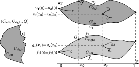
Let and be planar nearlattices and fix a planar diagram for each of them. By taking isomorphic copies if necessary, we can assume that . Let be distinct elements on the same (left or right) boundary chain of the same cell of , with respect to its fixed diagram, such that and is not the smallest element of the cell. Let be a coatom on the boundary of , with respect to its fixed diagram, again. Let be the poset with and the ordering defined by
Then is a planar poset.
Proof.
After reflecting one or two of our nearlattices across a vertical axis, we can assume that and are on the right boundary of the cell mentioned in the theorem and is on the right boundary of . The cell in question is dark grey in the second part of Figure 2. Choose a pointed contour inside the cell such that is the top of this pointed contour and ; see on the right of Figure 2. Also, choose another pointed contour such that the diagram of is inside it and ; see on the left of the figure. It follows from Lemma 3.4 that has a planar diagram inside such that and are at and . The union of this diagram and that of is a curved planar diagram of . Hence, is planar by D. Kelly’s theorem, (3.1). ∎
4. Substructures, qn-lattices, and jm-constraints
This section begins with some definitions that will be used later in the paper. Note in advance that even for lattices rather than nearlattices, the concepts we are going to introduce are distinct from those of partial lattices and weak partial sublattices discussed in Grätzer’s monograph [21].
For a nearlattice , the domain of the meet operation is
| (4.1) |
since , provided the set mentioned here is nonempty. The domain is, of course, . By reducing the domains, we obtain the following concept. By a partial jm-algebra we shall mean a partial algebra of type where and stand for binary partial operations; the letter j and m come from the names of operation symbols. We will adhere to the convention that
| each equality for a partial jm-algebra will mean that and , and similarly for the other partial operation. | (4.2) |
A partial jm-algebra with ordering is a structure such that is a poset and is a partial jm-algebra. (That is, we do not require that the partial operations are isotone.) The following concept is more subtle. Our guiding example is a nonempty subset of a nearlattice and the restrictions of the operations of to such that and analogously for .
Definition 4.1.
A qn-lattice is a finite partial jm-algebra with ordering such that the following five axioms hold for every ; convention (4.2) will be in effect.
-
(A1)
if , then and, dually, whenever .
-
(A2)
if and are comparable, then and .
-
(A3)
and, dually, .
-
(A4)
, and imply that . Dually, , and imply that .
-
(A5)
and imply that . Dually, and imply that .
The letters q and n in the name of qn-lattices comes from “quasi” and “near”. Clearly, every nearlattice is also a qn-lattice, and every qn-lattice is a partial jm-algebra with ordering. Since the notations and can mean various things like a nearlattice, a lattice, or a partial jm-algebra, it will be important to frequently specify the meanings of our notations.
Let and be partial jm-algebras with orderings. (In particular, they can be nearlattices or a qn-lattices.) We say that is a weak partial subalgebra of if its ordering is the restriction of that of to , ,
| , , | (4.3) |
and, in addition, and are the restrictions of to and to , respectively. In this case, is also said to be a weak partial subalgebra of . The adjective “weak” reminds us that the inclusions in (4.3) can be proper. If both and are qn-lattices, then we prefer to say that is a sub-qn-lattice of instead of saying that it is a weak partial subalgebra of . Let us emphasize that, by definition,
| a sub-qn-lattice is automatically a qn-lattice. | (4.4) |
For a qn-lattice ,
| (4.5) |
the only difference (apart from replacing by ) is that now we need rather than . As it is clear from (4.5), now a subuniverse is just a subset of without any structure on it. Thus, a qn-lattice can have much more sub-qn-lattices than , because a subuniverse can be the support set of several sub-qn-lattices. So the counterpart of (2.4) does not hold for qn-lattices. Having its subuniverses just defined, is also meaningful for a qn-lattice ; see Definition 2.1.
The following easy lemma, which is a particular case of Lemma 2.3 of Czédli [13], indicates the importance of our new concepts.
Lemma 4.2.
If is a sub-qn-lattice of a qn-lattice , then .
By a jm-constraint over a set we mean a formal equality or such that is a three-element subset of . If is a set of jm-constraints such that whenever and belong to then and dually, then is coherent. A coherent together with determine a partial algebra in the natural way: such that belongs to , similarly for , and the action of and in their domains are given by the jm-constraints in . If is understood, we speak about the partial algebra determined by . We are interested only in the following particular case.
Definition 4.3.
-
(i)
Let be nonempty subset of a qn-lattice . Let be a set of jm-constraints over such that each jm-constraint in is a valid equality in ; such a is necessarily coherent. Then is said to be a set of jm-constraints over compatible with . Note that the partial algebra determined by and is clearly a weak partial subalgebra of .
-
(ii)
By an -compatible set of jm-constraints we mean a set of jm-constraints over some such that is compatible with . In other words, is a collection of true equalities in .
-
(iii)
Over a subset of , let be a set of jm-constraints compatible with , and keep (4.4) in mind. The least sub-qn-lattice of such that all the jm-constraints in are valid equalities in this sub-qn-lattice is called the qn-lattice determined by over in . Here “least” means that whenever all the jm-constraints of are valid equalities in a sub-qn-lattice of , then is a sub-qn-lattice of .
-
(iv)
If is the collection of all elements occurring in the jm-constraints belonging to , then the reference to in the form “over ” is usually dropped and we speak of the qn-lattice determined by in . If every element of a qn-lattice occurs in a jm-constraint belonging to , then even the reference to is often dropped and we simply speak of the qn-lattice determined by ; however, then it should be clear from the context what is. This convention of not mentioning is typical when is given by its diagram.
-
(v)
If a qn-lattice is determined by and a diagram as in (iv) and the diagram contains dashed edges, then means any of the several qn-lattices determined so that we remove some of the dashed edges, possibly none of them, and make solid the rest of dashed edges, possibly none of them. In this case, a statement “ is not a sub-qn-lattice of a given qn-lattice ” means that “no matter which dashed edges are erased and which are made solid, the qn-lattice determined in this way is not a sub-qn-lattice of ”. Note that the dashed edges should not be confused with the dotted ones occurring later in the paper.
Example 4.4.
The following lemma is quite easy but it will be important in most of our arguments later.
Lemma 4.5.
If is a set of jm-constraints compatible with a qn-lattice over , , then the qn-lattice determined by over can be described as follows. We begin with the partial algebra determined by , and take , where is inherited from . Assume that, for some , is already given. If one of the axioms (A1)–(A5) is violated, then pick a pair and one of the axioms violated by this pair, and extend the domain of or by to get rid of this violation; let denote what we obtain in this way. Note that is a weak partial subalgebra of . If none of the axioms (A1)–(A5) is violated, which happens sooner or later by finiteness, then is the qn-lattice determined by over in .
Proof.
Since none of the axioms (A1)–(A5) is violated after the inductive procedure, is a qn-lattice. We need to show only that is a weak subalgebra of for all . We prove this by induction on . The case is evident. Assume that a weak subalgebra of for some . We can assume that is obtained from so that we got rid of a violation of (A4) or (A5), because the axioms (A1)–(A3) create no problem. If the first half of (A4) was violated then, with the notation taken from Definition 4.1, the induction hypothesis gives that and . Since , we can compute in as follows: . That is, . Hence, enriching the domain of with and letting results in a weak subalgebra of , and this subalgebra is . Duality takes care of the second part of (A4); however, then the following fact, which is a trivial property of infima, has also to be used:
| (4.6) |
A similar argument applies for (A5) since nearlattice operations are isotone. This completes the induction step and the lemma is concluded. ∎
Convention 4.6.
Given a nearlattice , let be an -compatible set of jm-constraints. By the -value of and, if and are understood from the context, the -value of the situation we mean where is a subset of such that the jm-constraints in are over and is the qn-lattice determined by over in . The least appropriate will be denoted by ; that is, is the collection of all elements that occur in jm-constraints belonging to . Hence, . If or the situation is clear from the context, then its -value will often be given by an equality like .
We formulate the following easy lemma, which will be used implicitly.
Lemma 4.7.
Convention 4.6 makes sense, that is, above does not depend on the choice of the subset of .
Proof.
Let be an arbitrary subset of such that is over . Clearly, . Since there is no stipulation on the elements of , we have that
completing the proof. ∎
Lemma 4.8.
If is a nearlattice and is an -compatible set of jm-constraints, then . In other words, then is at most the -value of the situation.
This lemma will be our main tool to show that is sufficiently small.
A computer program
Lemma 4.8 will be useful for our purposes only if we can determine the -values of many situations. Since that much work would be impossible manually, we have developed a computer program, using Bloodshed Dev-Pascal v1.9.2 (Freepascal) under Windows 10, to do it.
This program, called sublatts, is available from the author’s website;
to find it, look for the present paper in the list of publications.
The input of the program is an unformatted text file describing an -compatible set of jm-constraints and the corresponding poset ; see Convention 4.6. As its output, the program displays on the screen and saves it into a text file.
Together with the result, , the set is also displayed and saved.
Upon request (using the \verbose=true command), even the qn-lattice determined by
is displayed and saved. The algorithm implemented by the program is trivial.
Namely, by computing the for successively according to Lemma 4.5, the program determines the qn-lattice in the first step. In the second step, the program takes all the subsets of and counts those that are closed with respect to the partial operations of . It is clear from the second step that the running time depends exponentially on . Fortunately, the biggest we need for this paper is only 12, and the program computes for 101 many times
in half a second on a desktop computer with an Intel Core i5-4400 Quad-Core 3.10 GHz processor.
Note that an earlier program, which was crucial for the papers Czédli [13] and [14], could also be used here but that would require much more human effort. This is so because the above-mentioned first step is not built in the earlier program and the user has to make this step manually while preparing the input files. Note also that the concept of qn-lattices has been developed for the sake of this first step.
As a consequence of Lemma 4.7, note that if the input files gives a poset such that is a proper subposet of , then the program still computes but in a longer time. Note also the following. Even if the program can detect many types of errors in the input file, it is the user’s responsibility that the ordering should harmonize with the qn-lattice operations. However, in most of the cases, it will not cause an error if some edges are missing from the input; see (7.5) and Remark 7.8 later.
5. Excluding some qn-sublattices
In order to outline the purpose of this section, we need the following convention.
Convention 5.1.
For the rest of the paper, we assume that Theorem 2.2 fails and will denote a counterexample of minimal size . In particular, but is not planar. The notation will always be understood as a nearlattice (rather than, say, a qn-lattice).
We are going to prove several properties of until it appears that cannot exist; this will imply Theorem 2.2. We begin with the following easy lemma. As usual, a subnearlattice is proper if it is not the original nearlattice.
Lemma 5.2.
Every proper subnearlattice of is planar.
Proof.
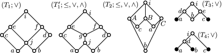
For later reference, we prove the following easy lemma. Not only the statement of the lemma but also its straightforward proof will often be referenced, explicitly or (later) implicitly. The qn-lattice in Figure 4 is defined as follows. Let be the collection of the following jm-constraints: , , for every with two distinct lower covers and , and for every with two distinct covers and . Then is the qn-lattice determined by .
Lemma 5.3.
If the join-semilattice given in Figure 4 is a subposet of a finite join-semilattice , then the nearlattice is a subnearlattice of the nearlattice , or the qn-lattice a sub-qn-lattice of the nearlattice .
Proof.
Unless otherwise stated by subscripts, the operations will be understood in . If , then let . Clearly, but and , because otherwise we would get or , which fail. Hence, we can replace by so that is (order-) isomorphic to . This allows us to assume that . Since , we have that . Hence, if , then we can replace by and we still obtain a poset isomorphic to . Thus, we can assume that . In the next step, based on symmetry (reflection across a vertical line), we can similarly assume that .
Next, if , then we replace by . Clearly, say, since , and we get an isomorphic poset. But now we have to show that an earlier achievement remains valid, that is, . This is clear again since and so . Hence, we can assume that . In the next step, we can also assume by symmetry. Note at this point that the order of our steps made so far was not arbitrary. Now, there are two cases.
First, if , then the equalities assumed so far are sufficient to say that the nearlattice is a subnearlattice of the nearlattice ; for example, . In other words, denoting by the collection of the equalities assumed, the qn-lattice determined by is the same as the nearlattice .
Second, if , then is a subposet isomorphic to . For example, because otherwise we would obtain that . The earlier equalities and form exactly the set of jm-constraints determining , and the lemma follows. ∎
Note in advance that the following lemma as well as many of the subsequent lemmas come with associated input and output files, which are available together with our computer program from the author’s website. Also, the extended version333This is the extended version. of the paper, available from arXiv or preferably from the author’s website, contains all the output files as appendices, and the input files can easily be obtained from the output files. Note also that, as a rule, the input and output files associated
with a lemma on are called LmXi.txt and LmXi-out.txt, respectively. Here is either a concrete natural number, or it is the letter “i” to denote a range of natural numbers. Once, to differentiate between two versions, we insert “a” or ‘b” right before ‘-out.text”. For example, Lemma 6.2 is a statement on (to be defined in due course) and the associated files are LmT4.txt and LmT4-out.txt while the files corresponding to the following lemma are LmSi.txt and LmSi-out.txt
The qn-lattices occurring in the lemma below have been defined in Example 4.4.
Lemma 5.4.
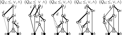
For , the qn-lattice is not a sub-qn-lattice of .
Proof.
The next property of that we are going to prove is the following.
Lemma 5.5.
The nearlattice is not a subnearlattice of .
The method of the proof below will be referenced as our parsing technique (with the help of our computer program). If the reader intends to check the output file LmT1a-out.txt, then the appendix given in Section 9 is worth reading.
Proof of Lemma 5.5.
Suppose the contrary. The notation given in Figure 4 will be in effect. The initial situation, to be denoted by (C), consists of and the operation table, that is, all equalities of the form and that hold in . Note that the input file need not and does not contain the whole operation table; it suffices to give a smaller set of jm-constraints such that the qn-lattice determined and is the nearlattice . In fact, it follows from Lemma 4.2 that even a set smaller than suffices if its -value is at most 83. Unfortunately, since now the -value of (C) is 84, which is too large for us, further work is necessary. Note the following principle in advance; it will frequently be used later, mostly without referencing it explicitly.
| (5.1) |
Since is planar but is not, there is an element . If all elements of belonged to the principal filter , then would be planar by Lemma 5.2 and thus would also be planar, which is not the case. Hence, we can assume that , and there are two cases, (C1) and (C2), to consider. As always in the rest of the paper unless otherwise explicitly stated, the operations will be understood in . Before going into details, let us agree that, in the whole paper, our convention for subcases is the following.
| (5.2) |
Note that, in order to increase readability, we insert a dot after every second character of when referencing (C).
(C1): and are incomparable, in notation, . Let . According to (5.2), now the situation is that of (C) together with , , and . Using our computer program with the input file LmT1a.txt, we obtain that the -value of the situation (C1) is ; see Convention 4.6. This does not exceed , so we are on the way to applying (5.1). (Alternatively, (5.1) excludes this case.)
(C2): . This case branches into two subcases.
(C2a): and . Then we can assume that since otherwise we can replace by . The -value of the situation is .
(C2b): and . Then . By (5.2), . But , whence . Using that , , and , it follows that or . By symmetry, we can assume that . Our argument splits according to the value of . First, if (C2b.1): , then . Second, if (C2b.2) is a new element, then and . By (5.1), (C2a) and (C2b) are excluded, whence there remains only one subcase at this level of parsing: or . By symmetry, it suffices to deal only with the former.
(C2c): . There are six subcases depending on . Note that and cannot be or , because they are not in the filter . If (C2c.1): is a new element, then , , , and . If (C2c.2): , then . For (C2c.3): , we have that . (C2c.4): gives that . The -value of (C2c.5): is . Finally, (C2c.6): yields that . By (5.1), (C2c) is excluded.
The lemma below is much easier; the qn-lattice has been defined right before Lemma 5.3.
The file associated with this lemma is LmT1b-out.txt .
Lemma 5.6.
The qn-lattice is not a sub-qn-lattice of .
Now, we are in the position to prove the following statement.
Lemma 5.7.
The poset , given by Figure 4, is not a subposet of the nearlattice .
Next, let be the seven-element qn-lattice defined by Figure 4 and determined by the set , , , , , of jm-constraints. Note that is redundant. Note also that is the join-semilattice freely generated by and that .
Lemma 5.8.
The qn-lattice is not a sub-qn-lattice of the nearlattice .
Proof.
Suppose the contrary. A routine argument, similar to the proof of Lemma 5.3, shows that , , and can be assumed, because otherwise we can easily enlarge , , and . So, in the rest of the proof, we add these three equalities to the set of jm-constraints defining the qn-lattice . So, from now on in the proof, is a nearlattice. Since is rather large, a whole hierarchy of cases have to be considered. Since is planar and it is a sub-qn-lattice of the nonplanar nearlattice , it follows that is nonempty. By Lemma 5.2, its filter is planar. Hence, is not included in this filter, because otherwise, as the glued sum of two planar nearlattices, would be planar. So, we can pick an element such that ; so either , or . If (C1): , then with , we obtain that .
(C2): ; this case splits into two subcases. First, assume that (C2a): , , and . Then the principal filter in is a lattice by (4.1). In this lattice, generate an 8-element boolean sublattice by, say, Grätzer [21, Lemma 73]. By the program or Czédli [13, Lemma 2.7], the -value of this boolean sublattice is 74, whereby (5.1) excludes (C2a). The conjunction of , and is also excluded, since it would lead to , contradicting the choice of . Hence, using that (C2a) has already been excluded, is incomparable with at least one of , , and . By symmetry, we can assume that . So, the second subcase is (C2b): . Since , we have that , where denotes a new element such that since . So there are exactly four subcases; namely, (C2b.1): , (C2b.2): , (C2b.3): , and (C2b.4): , but all of them is excluded by (5.1) since the corresponding -values are , , , and . (Note that (C2b.3) does not need a separate computation since it follows from (C2b.2) by – symmetry.) By (5.1), (C2b) is excluded and Lemma 5.8 is concluded. ∎
An element in a poset is meet irreducible if it has exactly on cover. If an element has at least two covers, then it is meet-reducible, no matter whether any meet resulting in is defined in the qn-lattice we deal with. Except for the singleton nearlattice (or join-semilattice), which is surely distinct from , a minimal element is either meet irreducible, or meet reducible.
Lemma 5.9.
Every minimal element of is meet reducible.
Proof.
Suppose the contrary, and let be a meet irreducible minimal element. Clearly, is a proper subnearlattice of . This subnearlattice is planar by Lemma 5.2. With reference to Corollary 3.5, is obtained from this subnearlattice, playing the role of , and the two-element lattice, acting as , by the construction described there. Hence, is planar by Corollary 3.5, which is a contradiction as required. ∎
6. Sub-nearlattices containing some minimal elements of
Although is a nearlattice, sometimes we need its join-semilattice reduct, ; for example, in the following lemma. The join-semilattice is defined by Figure 4, where the notations of its elements are also given.
Lemma 6.1.
The join-semilattice cannot be a subsemilattice of the join-semilattice so that and (the black-filled elements in the figure) are minimal elements in .
Proof.
Suppose contrary. Replacing by if necessary, we can assume that . By Lemma 5.9; has two distinct covers, and ; clearly, . Similarly, with distinct covers and of . Observe that
| (6.1) |
because a common cover of and would satisfy but then would contradict . By (5.1), we exclude case (C1): and since its -value is . Note, in advance, that (6.1) will also be valid for the rest of cases. Next, we deal with the case when exactly one of the previous two inequalities hold; by –-symmetry, this is case (C2): but . Let, say, . Observe that since otherwise would not hold. Hence, . We will not use because it may equal . Since and , we have that . If (C2a): is an “old element”, then (the only old element larger than ), , and . Otherwise, if (C2b): is a new element, then . Hence, (5.1) excludes (C2). The next case is (C3): and . Let, say, and ; we will not work with and . We still have that and . Similarly, and . At present, is the set of old elements; only from the old elements can be but need not be an upper bound of , and the same holds for . If both and are old elements, then (C3a): and . If only one of the two above-mentioned joins is a new element, then symmetry allows us to assume that (C3b): is new and is old, and then . Next, if (C3c): and are distinct new elements, then either (C3c.1): is a new element and , or (C3c.2): and . If (C3d): , then is a new element since (5.1) excludes (C3a), since , and . Thus, (5.1) completes the proof. ∎
The join-semilattice is defined in Figure 4.
Lemma 6.2.
The join-semilattice cannot be a subsemilattice of the join-semilattice so that , and (the black-filled elements in the figure) are minimal elements in .
Proof.
Suppose the contrary. By Lemma 5.9, there are elements such that and are distinct covers of , the elements and are those of , and and are those of . Let us agree that , whereby and we can always use the elements , , and . However, , , and will be used only if they are distinct from , , and , respectively. This means that mostly when, say, occurs in the argument, then is assumed even if this is not mentioned again, and similarly for and , which are mentioned typically when they are distinct from . Note that if, say, both and are used “at ”, then the jm-constraint is included in the situation, and similarly at and . The inequalities , , and are permanent in the situations but if, say, is the only occurrence of , then the element could be omitted without changing the -value. Now, the parsing tree will be larger than in the previous proofs. Note at this point that whenever a case is excluded, then this always happens by (5.1) even if (5.1) is not referenced. Furthermore, when a new case or subcase begins, all the previous ones have already been excluded even if this is not mentioned.
(C1): and . More precisely, has two distinct covers in and they are denoted by and . Then, since , we have that and . As we have already mentioned, .
(C1a): . Now, we have to look at , and then .
(C1a.1) . Then and . Observe that none of and covers , because otherwise this cover of would be greater than or equal to , which would contradict . Now if (C1a.1a): , then and imply that and we have that ; otherwise (C1a.1b): exists, , and . Hence, by (5.1), (C1a.1) is excluded.
(C1a.2): . That is, , and we can chose outside by – symmetry; will not be used because we do not know if it is equal to or distinct from . Since , we obtain easily that . Observe that is either , the only old element larger than , or a new element .
(C1a.2a): . First, (C1a.2a.1): yields that and . Second, assume that one of and , say , is not in , so (C1a.2a.2): , that is, . Now (C1a.2a.2a): yields that while (C1a.2a.2b): , a new element, leads to . Hence, by (5.1), (C1a.2a) is excluded.
(C1a.2b): is a new element. First, let (C1a.2b.1): . Then (C1a.2b.1a): gives that while (C1a.2b.1b): and, say, yields to and . Hence, by (5.1), (C1a.2b.1) is excluded. Second, let (C1a.2b.2): . Then either (C1a.2b.2a): and , or say (C1a.2b.2b): and we obtain that and . By (5.1), (C1a.2b.2) is excluded. Third, if (C1a.2b.3): , then is a new element and . Hence, (C1a.2b), (C1a.2), and (C1a) are excluded.
(C1b): is a new element.
(C1b.1): and . Then and , whence this case is excluded.
(C1b.2): and, say, . Then , and we continue similarly to (C1a.2).
(C1b.2a): (the only possibility that is an old element). Then (C1b.2a.1): gives that and . Otherwise, if , then we can assume that , so (C1b.2a.2): , leading to . Hence, (C1b.2a) is excluded.
(C1b.2b): is a new element. Now (C1b.2b.1): gives that , (C1b.2b.2): leads to , and (C1b.2b.3): yields that is a new element and . Hence, (C1b.2b) is excluded, and so are (C1b), and (C1).
(C2): . (Apart from – symmetry, this is the opposite of (C1) even if .) Then is a new element and .
(C2a): . Then and . As in case (C1a.1), none of and covers . There are two subcase. First, let (C2a.1): . If (C2a.1a): , then and . Otherwise (even if ) we can assume that (C2a.1b): , which gives that . Hence, (C2a.1) is excluded. Second, if (C2a.2): is a new element, then . Thus, (C2a) is excluded.
(C2b): and, say, . Then . Depending on , there are three subcases, because only two of the old elements belong to . First, let (C2b.1): . Then either (C2b.1a): , whence and , or (C2b.1b): and, say, , whence and . Hence, (C2b.1) is excluded. Second, let (C2b.2): . Then either (C2b.2a): , so and , or (C2b.2b): and, say, , whereby and . Hence, (C2b.2) is excluded. Third, if (C2b.3): is a new element, then either (C2b.3a): , , and , or (C2b.3b): allows only three old elements larger than and, thus, splits into (C2b.3b.1): with , (C2b.3b.2): with , (C2b.3b.3): with , and (C2b.3b.4): , a new element, with . Hence, (C2b.3) is excluded, and so are (C2b), and (C2). Finally, (5.1) completes the proof of Lemma 6.2. ∎
7. Sub-qn-lattices with entries and anchors
By Czédli [13], if is a finite lattice (not only a nearlattice) that satisfies , than is planar. From our perspective, this result is equivalent to the following lemma; see Convention 5.1 for the notation.
Lemma 7.1 (Czédli [13]).
The nearlattice has at least two minimal elements.
If has only two minimal elements, than condition (7.1) below clearly holds.
Definition 7.2.
With the assumption that
| (7.1) |
we introduce the following notations and concepts. The filter is called the kernel of . For a minimal element of , the set is the wing of . An element is called an -entry if it has a lower cover in the -wing . Let us emphasize that is not an -entry. If is an -entry and is a lower cover of , then is an -anchor of and the edge is an -bridge. By an entry, an anchor, or a bridge, we mean an -entry, an -anchor, or an -bridge, respectively, for some minimal element .
Lemma 7.3.
Assuming (7.1), let be a minimal element of . Then every wing is an order ideal (also known as a down-set). The wing is the set of all such that is the only minimal element of the principal ideal . If is also a minimal element and , then holds for all and ; in particular, then and no -anchor is a -anchor. Finally, an element of is either in the kernel , or it is in a uniquely determined wing .
Proof.
Since is is a filter also in , it is evident that is an order ideal. The second part follows from the fact every element above two distinct minimal elements are in the kernel . If, in spite of the assumptions, and are comparable, say, , then would lead to and so , a contradiction. Finally, if , then take a minimal element of such that . If is the only such element, then . Otherwise, there exists a minimal element , and yields that . ∎
Lemma 7.4.
Assuming (7.1), let be a minimal element of , and let be a minimal -entry with an -anchor . Then for every , if , then .
Proof.
Let be a maximal chain in the interval . Since wings are order ideals and , we have that . So, but . Hence, there is a least subscript such that but . Since , we have that . Thus, . Now if , then is an -entry with -anchor , but this is impossibly since and is a minimal -entry. Hence, and so , that is, . Using this inequality and , we obtain that , as required. ∎
The general assumption for the rest of this section, which is stronger than (7.1), is the following.
| has exactly two minimal elements, and ; the notations and concepts given in Definition 7.2 will be in effect. | (7.2) |
Note that in the input and output files, we write and instead of and , respectively. Consider the qn-lattice determined by Figure 5 and
| (7.3) |
Lemma 7.5.
Assuming (7.2), the qn-lattice cannot be a sub-qn-lattice of so that , , and the thick edges are bridges.
Remark 7.6.
Observe that an equivalent assumption for Lemma 7.5 is that , , and the thick edges correspond to covering pairs (that is, edges) in the nearlattice . Indeed, then the jm-constraint guarantees that is , and since the order embedding preserves incomparability, it follow easily that the covering pairs corresponding to the thick edges are bridges in . Conversely, we know from Definition 7.2 that bridges are covering pairs. Without separate mentioning, analogous observations hold for the rest of the lemmas where bridges are mentioned.
Proof of Lemma 7.5.
Suppose the contrary. If , then we modify to . Similarly, . Since thick edges correspond to bridges and, thus, to coverings, see Remark 7.6, we obtain easily that since . So, from now on, the equalities from the set hold. Therefore, we can assume that is determined by the set of constraints. However, we will occasionally rely on the equality and the inequalities provided and . First, we show that
| (7.4) |
Suppose the contrary and take an that violates (7.4); then , , , and . First, assume that (C1): . If (C1a): , then is a new element, gives that , and excludes (C1a) by (5.1). Second, assume that (C1b): . Then since there are only two minimal elements, whence . Since contains only three old elements, we have that (C1b.1): and , or (C1b.2): and , or (C1b.3): and , or (C1b.4): is a new element and . Hence, by (5.1), (C1b) and (C1) are excluded. Therefore, since and have been assumed, . Second, assume that (C2): (in addition to ), and take . Since and , there are only four possibilities for ; namely: (C2a): , (C2b): , (C2c): , and (C2d): is a new element. Since their -values are , , , and , respectively, (5.1) excludes (C2). Combining this fact with and , we obtain that . But then , and form a contradiction, which proves (7.4).
Clearly, for every , the poset is planar. Therefore, we can pick an element ; it follows from (7.4) that . If (C3) , then we let to obtain that , which is impossible. This fact combined with gives that . Since but , we obtain easily that , , and ; for example, would lead to , which would contradict . By (7.4), if , then either , contradicting , or , leading to the contradiction , or , contradicting . Hence is in , but it is neither , nor since and . Similarly, is in but and is in but . Hence, (C4): , , , and completes the proof by (5.1). ∎
Lemma 7.7.
Assuming (7.2), the qn-lattice cannot be a sub-qn-lattice of so that , , the thick edges are bridges, and is a minimal -entry.
Proof.
The following remark will be useful in the proofs of several statements.
Remark 7.8.
Assume that and are posets such that for every , if , then . Let be a set of jm-constraints over . For , let be the qn-lattice determined by and (the diagram of) . Then . In particular, if we remove an edge from a diagram, then the -value of the situation (determined by a given set of jm-constraints) increases, provided we do not make use of some new incomparability (that is, such that or ).
The statement of this remark is trivial: if we have less comparable pairs, then the axioms (A1)–(A5) from Definition 4.1 bring less jm-constraints in, so more subsets will obey the jm-constraints, whence increases. As we know from (5.1), our permanent intention is show that the -values are small enough. Hence, the practical value of Remark 7.8 is the following.
| (7.5) |
Of course, if the -value becomes too large after deleting an edge (or ), then our attention turns to the new join , which is either an old element, or a new one, and even to if it exists.
Consider the qn-lattice determined by from (7.3) and Figure 5; the dotted edge is taken into account.
Lemma 7.9.
Assuming (7.2), the qn-lattice cannot be a sub-qn-lattice of so that , , and the thick edges are bridges.
Proof.
Suppose the contrary. We can replace and by and , respectively. Note that now may fail; the purpose of the dotted edge is to remind us of this fact. Since , from and we obtain that . Similarly, we obtain that . Hence, after deleting the dotted edge from the diagram and letting , we can assume that is determined by ; see (7.3) and (7.5). Clearly, since otherwise we would get that by transitivity. Hence, based on the relation between and , there are two main cases. First, if (C1): , then and the -anchor are in , so we can add their meet to , we have that (since ) and (since and ), and we obtain that . Hence, (5.1) excludes (C1).
Second, we assume that (C2): . Depending on , there are two subcases. We begin with (C2a): , which splits again depending on . The analysis for (C2a.1): runs as follows. Since the situation at present describes a planar qn-lattice and remains planar for every , there exists an additional element . So or . If (C2a.1a): , then letting , . If (C2a.1b): , then, using that , either (C2a.1b.1): and so with , or (C2a.1b.2): , when since . So (C2a.1b.2a): with , or (C2a.1b.2b): and so and , or (C2a.1b.2c): and with and . (Note that with playing the role of , even (C2a.1b.2b) excludes (C2a.1b.2c).) At this stage, (5.1) excludes (C2a.1). Since (C2a.2): is also excluded by its -value , (C2a) is impossible. So is (C2b): by its . By (5.1), the proof of Lemma 7.9 is complete. ∎
Lemma 7.10.
Assuming (7.2), the qn-lattice cannot be a sub-qn-lattice of so that , , the thick edges are bridges, and is a minimal -entry.
Proof.
Suppose the contrary. As usual, we can replace and by and , respectively. But note then may fail; this is what the dotted edge indicates. However, since otherwise we would obtain that . By Lemma 7.4, . Using that , , , and , we obtain easily that and . Therefore, after letting and removing the dotted edge from the diagram, see (7.5), we can assume that is determined by ; see (7.3). If (C1): , then letting and adding to , we obtain , which is excluded by (5.1). So let (C2): . Then either (C2a): , the only element of , and , or (C2b): and . Thus, (5.1) applies and completes the proof. ∎
Next, let be the qn-lattice determined by the set
of jm-constraints and Figure 5; see Definition 4.3(v) about the dashed edge.
Lemma 7.11.
Assuming (7.2), the qn-lattice cannot be a sub-qn-lattice of so that , , and the two thick edges are bridges.
Proof.
Suppose the contrary. As usual, see the proof of Lemma 7.5 or that of Lemma 7.10, we can assume that and . Since and , see Remark 7.6, we also have that and . The parsing runs as follows.
(C1): . There are two subcases. First, if (C1a): , then either (C1a.1): and , or (C1a.2): and . Second, if (C1b): , then either (C1b.1): and , or (C1b.2): (where is distinct from because otherwise we would obtain that ) and . Hence, (C1) is excluded by (5.1).
(C2): . Again, there are two subcases. First, if (C2a): , then either (C2a.1): and , or (C2a.2): (but since ) and . Hence, (C2a) is excluded. Second, if (C2b): , then either (C2b.1): and , or (C2b.2) , which is distinct from since otherwise would contradict , and . Hence, (C2b) and (C2) are excluded, and (5.1) completes the proof of Lemma 7.11. ∎
Next, we consider the qn-lattice determined by the set of jm-constraints, see (7.3), and the diagram given in Figure 5; the diagram is understood as follows. The dotted edges stand for and , but they are not necessarily coverings and, later in the proof, we can drop and . According to Definition 4.3(v), the dashed edges mean that either , or , and similarly, either , or . Since there are four possibilities to choose the actual meanings of the dashed edges, we have defined four distinct versions of ; the following lemma is stated for all of them.
Lemma 7.12.
Assuming (7.2), no version of the qn-lattice can be a sub-qn-lattice of so that , , the thick edges are bridges, is a minimal common -and--entry, is a minimal -entry, and is a minimal -entry.
Proof.
Suppose the contrary. As usual, see the proof of Lemma 7.5 or that of Lemma 7.10, we can assume that and . Then, of course, the two dotted edges in the figure need not mean comparability. By Lemma 7.4, . Since the upper two thick edges stand for coverings, and . (Alternatively, and similarly for .) Therefore, after letting , we can assume that is determined by . Even if none of the dotted and dashed edges is considered, . (Otherwise, if some of these edges are also considered, can be slightly smaller; see Remark 7.8 and (7.5); for example, if all these four edges are taken into account.) Finally, (5.1) completes the proof of Lemma 7.12. ∎
Next, let be the qn-lattice determined by Figure 6 and the set
| (7.6) |
of jm-constraints; note that even if the dashed edge is removed from the figure, we still assume that . The general assumption for the following five lemmas is that
| (7.7) |
Lemma 7.13.
If the nearlattice has exactly two minimal elements, then the qn-lattice cannot be its sub-qn-lattice so that (7.7) holds.
Proof.
Suppose the contrary. As usual, see the proof of Lemma 7.5 or that of Lemma 7.10, after replacing and by appropriate meets if necessary, we assume that and ; however, then need not hold. Lemma 7.4 allows us to assume that . Finally, using that (or that ), we obtain that . Hence, the initial set of jm-constraints is
Observe that is impossible since it would lead to by transitivity. Hence, based on the relation between and , there are only two cases. First, if (C1): , then either (C1a): , the only element in , and , or (C1b): is a new element and . Second, if (C2): , then , , and . Thus, (5.1) completes the proof. ∎
Lemma 7.14.
If the nearlattice has exactly two minimal elements, then the qn-lattice cannot be its sub-qn-lattice so that (7.7) holds.
Proof.
Suppose the contrary. Let . By the same reasons as in the proof of Lemma 7.13, we can work with the initial set
again; we have to drop the assumption that but we add that and . Then completes the proof. ∎
Lemma 7.15.
If the nearlattice has exactly two minimal elements, then the qn-lattice cannot be its sub-qn-lattice so that (7.7) holds.
Proof.
Suppose the contrary. Compared to the previous two proofs, the only difference is that now . Since , the meet exists. Using that , (C1): with , (C2): with , and (C3): with are the only cases. Hence (5.1) applies. ∎
Lemma 7.16.
If the nearlattice has exactly two minimal elements, then the qn-lattice cannot be its sub-qn-lattice so that (7.7) holds.
Proof.
Lemma 7.17.
If the nearlattice has exactly two minimal elements, then the qn-lattice cannot be its sub-qn-lattice so that (7.7) holds.
8. Our lemmas at work
Armed with the lemmas proved so far, we are ready to set off to prove our result.
Proof of Theorem 2.2.
It has been proved in Czédli [13] that for every , there exists an -element nonplanar lattice , which is also a nearlattice, such that . Hence, the second part of the theorem needs no proof here. We also know from [13] that whenever is a finite lattice with , then this lattice is planar. Therefore, it suffices to prove the first part of the theorem only for nearlattices that are not lattices. For the sake of contradiction, suppose that the theorem fails. Thus, Convention 5.1 will be in effect. So the final target is to show that does not exist.
First, assume that has at least three minimal elements, and pick three distinct minimal elements, , , and . Let
It follows from Lemma 5.8 that . Similarly, Lemmas 6.1 and 6.2 yield that . Hence, ; this means that for any three distinct minimal elements,
| (8.1) |
Now let be an additional minimal element. Applying (8.1) first to the triplet , and then to , we have that , and it follows that any two distinct minimal elements of have the same join. Therefore, from now on, we can and we will rely on Definition 7.2. Next, we claim that
| for every minimal element , there exists an -entry. | (8.2) |
Suppose the contrary. Then is the interval , and it is planar by Lemma 5.2. Observe that now the subset is a subnearlattice. In order to see this, let ; then and for some minimal elements and distinct from . The intersection (if exists) cannot belong to , because otherwise and would give that , we would obtain similarly, whence would imply that is outside . Since is an order ideal by Lemma 7.3, is clearly outside , and we conclude that is, indeed, a subnearlattice. As a proper subnearlattice, it is planar, again by Lemma 5.2. With , , and playing the role of , and , Corollary 3.5 is applicable and implies that is planar, which is a contradiction proving (8.2).
Clearly, for every minimal element of ,
| if is an -entry and is an -anchor of , then , | (8.3) |
since this follows from , , and . Next, we claim that
| (8.4) |
For the sake of contradiction, suppose that (8.4) fails. Let and be an -anchor of and a -anchor of , respectively. Then and by (8.3). We cannot have that since otherwise we would obtain that . Also, , because otherwise . Symmetrically, and . These considerations show that the subposet of is isomorphic to ; see Figure 4. This contradicts Lemma 5.7 and proves (8.4).
Next, we claim that
| has only two minimal elements; let us agree that they will be denoted by and . | (8.5) |
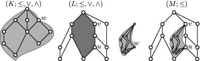
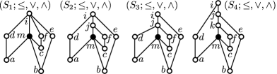
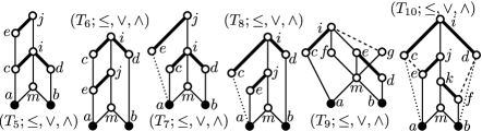
Suppose the contrary, and let , , and be three distinct minimal elements. Pick an entry for each of them. We know from (8.4) that these entries form a chain. Since they are not necessarily distinct, the entries in question form a one-element, a two-element, or a three-element chain . Let , , and be an -anchor, a -anchor, and a -anchor of the corresponding entry, respectively, and define , , and . Since is an order ideal, . Similarly, and . By Lemma 7.3, is a three-element antichain. By (8.3), it is clear that, up to permutation of the elements , the subset of forms a sub-qn-lattice isomorphic to one of the qn-lattices , , determined by Figure 3 and in Example 4.4. But this is a contradiction by Lemma 5.4, which proves (8.5).
Next, we are going to show that
| and do not have a common entry, | (8.6) |
that is, no -entry is a -entry. Suppose the contrary, and let be a minimal common entry of and . In fact, since any two common entries are comparable by (8.4), is the least common entry of and . Pick an -anchor and a -anchor of . By Lemma 7.3, . Since is planar by Lemma 5.2 and it is a lattice, we can fix a planar diagram of . In this diagram, the kernel of is a region by Kelly and Rival [46, Lemma 1.5]. If was in the interior of this region, then no lower cover of could be outside by Kelly and Rival [46, Lemma 1.2]. But we know that and are lower covers of outside , and we conclude that
| is on the boundary of , | (8.7) |
with respect to the fixed diagram . By left-right symmetry, we can assume that
| is on the left boundary chain of . | (8.8) |
We claim that
| (8.9) |
For the sake of an additional contradiction, suppose that is the only -entry and the only -entry. In order to prepare a forthcoming statement, (8.11), note that the argument beginning here and lasting up to (8.11) will use less assumption than what we have at present; it will use only that is a minimal -entry.
Let , let be the rightmost lower cover of that belongs to , and for , let be the rightmost lower cover of in the diagram , provided is not the smallest element . Since is an order ideal, is automatically in . Denote the finite chain by . We also define another chain, , as follows. Let , and let be the unique lower cover of on the left boundary of . That is, by (8.8), is the leftmost lower cover of in . Yet another way to define is to say that is the leftmost lower cover of that is to the right of . So, and are neighbouring lower covers of . As long as , let be the leftmost cover of in the diagram . Let be the first place where, going downwards, the chains and intersect first. (This place exists, because the two chains intersect at .) Let and . By Kelly and Rival [46, Lemma 1.5], the interval is a region in . The chains and divide this region into three parts; with our temporary terminology, into the left part of consisting of the elements on the left of (including the elements of ), the right part of consisting of the elements on the right of (including the elements of ), and the middle part of consisting of those elements that are simultaneously strictly on the right of and strictly on the left of . Of course, everything here is understood modulo the fixed diagram of . We claim that middle part of is empty. For the sake of contradiction, suppose that is an element of the middle part. Then there is a maximal chain in . Since and are neighbouring lower covers of , is either in the left part of , or in the right part. However, if is on the left part of , then the whole remains in the left part, because each of the is the rightmost lower cover of for and because cannot “jump over” by Kelly and Rival [46, Lemma 1.2]. Similarly, if is in the right part of , then so is the whole . So is either entirely in the left part, or entirely in the right part, whereby cannot contain the element , which is in the middle part. This contradiction shows that the middle part is empty and we have seen that
| is a cell. | (8.10) |
Next, we show that but ; then, in particular, it appears that is not the least element of the cell given in (8.10). Since and is an order ideal by Lemma 7.3, and yield that . Clearly, but is not in . So there is a least subscript such that but . Since we are in , the diagram of , we know that . Since would lead to and , we obtain by Lemma 7.3 that . By the definition of , is at least 1 and so . If we had that , then would be an -entry with -anchor , but this is not possible since is a minimal -entry. Hence . But , and we conclude that , as required. By the definition of and , the for are on the right boundary chain of . Below, for later reference, we summarize what we have just shown.
| (8.11) |
Next, we resume the latest assumption that is the only -entry and the only -entry. However, we will not always fully exploit this assumption. For the sake of a later reference, note in advance that
| for the validity of the forthcoming (8.13), (8.14), and (8.15), it suffices to assume that is the unique -entry, | (8.12) |
that is, we will not use for a while that is also the unique -entry. We claim that
| whenever , then . | (8.13) |
Indeed, take a maximal chain in the interval , and assume that , that is, . Since but , so , there is a smallest subscript such that but . Since but , we know from Lemma 7.3 that is not the only minimal element in . Hence, and . This fact and give that is a -entry. Since but , we obtain that , whereby is the same as , the only -entry. Hence, and . On the other hand, by the choice of our maximal chain, , whence . Thus, , and we conclude (8.13). Next, armed with (8.13), we claim that
| is a subnearlattice of . | (8.14) |
In order to prove this, assume that and ; we need to show that (which exists since ) and are in also in . Since is a chain but is not, at least one of and is not in . So, we can assume that, in addition to , and . Since is an order ideal, is in ; suppose that is not. Then by Lemma 7.3, whereby follows from (8.13). This proves (8.14). By Lemma 5.2,
| is a planar nearlattice. | (8.15) |
If we had an element such that , then (8.13) would give that , which would contradict the inequality . Hence, is a coatom in the nearlattice . Letting play the role of , it follows from Corollary 3.6, (8.8), and (8.11) that is planar, which is a contradiction. Completing the “encapsulated indirect argument”, this proves (8.9).
Next, we continue our argument towards (8.6); is still the least common entry. We claim that
| (8.16) |
Suppose the contrary. Then there exist a minimal -entry and a minimal -entry such that and . Since is the least common entry, is not a -entry and is not an -entry. Hence, these two entries, and , are distinct. Also, they are comparable by (8.4). Since and play a symmetric role, we can assume that . In addition to the already picked -anchor and -anchor of the common entry , choose an -anchor of and a -anchor of . We know from (8.3) that , , , and . Since , it follows that , that is, or . Similarly, or . Of course, each of and is incomparable with each of and by Lemma 7.3. These facts show that, in , the subset forms a sub-qn-lattice isomorphic to (one of the four versions of) . Since this is impossible by Lemma 7.12, we have proved (8.16).
We know from (8.9) that is not the only entry. Below, in order to prove (8.6), we are going to deal with two cases; namely, either is a minimal entry, or it is not minimal.
First, assume that is a minimal entry, that is, neither an -entry, nor a entry can be smaller than . Since any other entry is comparable with by (8.4) and there exists another entry by (8.9), and since and play a symmetric role, we can assume that there exists an -entry such that . (It may but need not happen that is also a -entry.) Let be an -anchor of . Few lines after (8.6), we mentioned that . Lemma 7.3 gives also that . Since and by (8.3), . So or . Using the just-mentioned consequences of (8.3) and depending on whether or , the qn-lattice or the qn-lattice is a sub-qn-lattice of so that its minimal elements are and and its thick edges are bridges, but this is impossible by Lemmas 7.5 and 7.9.
Therefore, since the opposite case has just been excluded, is not a minimal entry. By the – symmetry, we can pick an -entry such that . It follows from (8.16) that is a minimal -entry. Pick an -anchor of . In addition to , Lemma 7.3 gives also that . By (8.3), the equalities and , and hold; the first two of them together with yield that or . Hence, either the qn-lattice , or the qn-lattice is a sub-qn-lattice of , but this is impossible by Lemmas 7.7 and Lemmas 7.10. This proves the validity of (8.6).
By (8.2), there are at least one -entry and at least one -entry. We claim that
| there are at least two -entries or at least two -entries. | (8.17) |
(This statement should not be confused with (8.9) where the existence of a common entry was assumed.) For the sake of contradiction, suppose that (8.17) fails. Let and be the unique -entry and -entry with -anchor and -anchor , respectively; see, for example, in Figure 5. We know from (8.4) that and are comparable. Furthermore, they are distinct by (8.6). Thus, using that and play a symmetric role, we can assume that . As in (8.7) and (8.8), we can assume that is on the left boundary chain of , with respect to the fixed diagram of . Letting play the role of , it follows from (8.12) and (8.15) that is a planar nearlattice. (In fact, it is a lattice.) If is also on the left boundary of , then the argument just after (8.15), tailored to the present notation by letting play the role of , shows that is planar, which is a contradiction. If is on the right boundary chain of , then the planarity of and that of trivially imply that is planar, which is a contradiction again. Therefore, is not on the boundary of , with respect to the fixed planar diagram . In other terms, being not on its boundary, is in the “interior” of . Hence, if we add to the right boundary chain of , which is a maximal chain, what we obtain is no longer a chain. This means that there is element on the right boundary chain such that . It is visually clear and follows rigorously from Kelly and Rival [46, Proposition 1.6] that is to the left of , that is, is to the right of . By left–right symmetry, there is an element on the left boundary chain of such that is to the left of . By an unpublished result of J. Zilber, see Kelly and Rival [46, Proposition 1.7], “left” is transitive and implies incomparability. Thus, is to the left of and is an antichain. Observe that and are comparable since both belong to the same (left boundary) chain, but since otherwise we would get that . Thus, . By (8.3), we have that forms a sub-qn-lattice of isomorphic to ; the meaning of the dashed edge in Figure 5 now depends on whether in or not. But this contradicts Lemma 7.11. Therefore, we conclude the validity of (8.17).
Based on (8.2), (8.4), (8.6), and (8.17), we know that, apart from –-symmetry,
| (8.18) |
Note that there can be more -entries and -entries, and an entry can have more anchors than those mentioned in (8.18). However, we obtain by comparing (8.3) and (8.18) with (7.6), (7.7), and Figure 6 that one of the qn-lattices , , is a sub-qn-lattice of so that (7.7) holds. But this is a contradiction by Lemmas 7.13, 7.14, 7.15, 7.16, and 7.17. Now that all possible cases have led to contradiction, it follows that does not exist. This completes the proof of Theorem 2.2. ∎
When reading the following proof, Kelly and Rival [46] or Czédli [13, Theorem 2.5], where the Kelly-Rival Theorem is cited, should be near; at the time of this writing, both of these two papers are freely downloadable.
Proof of Remark 1.3.
By Czédli [13, Remark 1.3], it suffices to show that whenever is a nearlattice with at least two minimal elements and , or and , then is planar. Suppose the contrary, that is, either , or and , and is nonplanar. Then the lattice we obtain from by adding a smallest element is nonplanar either. If , then this nonplanar lattice is necessarily the eight-element boolean lattice by the Kelly–Rival Theorem, see [46], and then is in Figure 4, which is planar. If , then it is straightforward to see by the Kelly–Rival Theorem that there are two possibilities. The first possibility is that is one of the nine-element lattices in Kelly and Rival’s list and then , which is obtained from this lattice, is planar simply because only minimal nonplanar lattices are included in the list. The second possibility is that the eight-element boolean lattice is a subposet of ; let be the unique element of . If is the smallest element of , then with by Czédli [13, Lemma 2.7], whereby this case is excluded.
If is a doubly irreducible element of , then and is a planar nearlattice, since it is seven-element, and it is trivial and it follows also from Corollary 3.5 that is planar, too.
We are left with the situation when is either join-reducible, or meet-reducible. It is easy to see that cannot be doubly reducible since there are no antichains and in such that for all . First, assume that is join-reducible. Then in such that and where is the join of and in . Assume that . Since there is only a single two-element antichain such that in , it follows easily that is a nonzero doubly irreducible element in . Hence, letting play the role of in the previous case, we obtain that is planar. Motivated by in Figure 4, it is not hard to draw a planar diagram for if . The analogous details for the case when is meet-reducible are omitted. ∎
9. Appendix 1: notes on our data files
How to test or create these data files
In general, an input file of our program parses a whole hierarchy of subcases. Since, for each subcase, the file has to repeat all jm-constraints of the parent case(s), the input file and also the output file are often considerably longer than the proof of the corresponding statement given in Sections 5–7. Since long files threaten with typing errors and the repeated use of the copy-paste function of our word processor without some easy-to-follow strategy threatens with even more involved errors, it is worth outlining a method that reduces the chance of these errors. The point is that instead of proofreading a long output file, we can economically create an input file by following the corresponding proof from Sections 5–7 and implementing a standard method of computer science to our work with the help of a word processor. This method is for listing the leaves of a tree by means of using a first in, first out data buffer (also called FIFO).
Roughly saying, we begin with a short text file describing the initial case (C); at this moment, this description is the first half of the file and the second half consists of a single comment line like \P0. Then we keep modifying the first half towards the required input file while using the second part as a FIFO. When the second half becomes empty, the first half is the input file. After describing the algorithm below, its functioning will be explained for the tree of subcases of the (main) case (C) given in Figure 7.
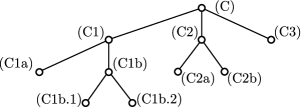
Algorithm 9.1.
-
(i)
Start with “ ”. Here is the end-of-file symbol, refers to the main case. The encircled 0 after the main case means that none of its subcases has been processed yet. The underlining means the position of the “cursor” in the text file we are creating. Also, the text before the cursor is the “first part” of the file, while the text after the cursor is the “second part”. Note that as long as the file is not finished, it contains exactly one underlined encircled number, which is always the first encircled number; we will refer to this number as the cursor or, shortly, . The case preceding the cursor will be denoted by . (At present, is the empty string.)
-
(ii)
If there is no cursor, then the input file is ready and the algorithm terminates. Otherwise, the first encircled number will be the cursor; underline it and go to the following step below.
- (iii)
- (iv)
- (v)
- (vi)
When working with the text file, then we write “\enddata” and a comment line “\Pc” instead of and , respectively, while (C) corresponds to the text starting with the last “\beginjob” command and ending with the “\endofjob” command before the cursor.
For the situation given by Figure 7; Algorithm 9.1 runs as follows.
| (9.1) | |||
| (9.2) | |||
| (9.3) | |||
| (9.4) | |||
| (9.5) | |||
| (9.6) | |||
| (9.7) | |||
| (9.8) | |||
| (9.9) | |||
| (9.10) | |||
| (9.11) | |||
| (9.12) | |||
| (9.13) | |||
| (9.14) | |||
| (9.15) | |||
| (9.16) | |||
| (9.17) | |||
| (9.18) | |||
| (9.19) | |||
| (9.20) |
For example, we have obtained (9.15) from (9.14) by replacing the string by the string . At the end, (9.20) lists the leaves of the tree in Figure 7 from left to right.
Note that although Algorithm 9.1 is good to organize our work and to see when a case has to be split into subcases, it needs the user’s decision what these subcases should be. Also, it is the user who has to prove that a subcase is meaningful; for example the user but not the computer verifies whether a new element occurring in the subcase is really distinct from previous elements.
A sample input file
Below, we give the input file LmQ4.txt in connection with Lemma 7.16. Since it contains only two cases, Algorithm 9.1 is not used. Command names begin with “ \ ”; in particular, “\P” means (and begins) comment lines to be printed in the output file. In a line, everything after a “ % ”
character is also a comment but it will not be printed. When listing edges and constraints, comments begin with “\w”; these comments are written in the output file. The lattice operations are denoted by (join) and (meet). The second line of the file, beginning with “ % ”,
is superfluous; it was used as a “mile stone” to avoid oversized lines.
\P Version of August 17, 2019
%                                                             E
\verbose=false
\subtrahend-in-exponent=8
\operationsymbols=+* % This command is obligatory.

\beginjob
\name
LmQ4/C1 d*m=a
\size
9
\elements
abmcdeijk
\edges
ac am be bm ci dj ek ij jk mi
 ad \w C1
\constraints
a+b=m c+m=i d+m=j e+m=k, c*m=a e*m=b b+d=j e*j=b e*i=b
 d*m=a \w C1
\endofjob

\beginjob
\name
LmQ4/C2 d*m=:x>=A
\size
10
\elements
abmcdeijkx
\edges
ac am be bm ci dj ek ij jk mi
 xd xm
\constraints
a+b=m c+m=i d+m=j e+m=k, c*m=a e*m=b b+d=j e*j=b e*i=b
 d*m=x x+b=m
\endofjob

\P Also done: LmQ4/C (all cases)
\enddata
10. Appendix 2: output files
This appendix presents the output files of our computer program. These files are integral parts of the proof of the main result of the paper; they are given in the following order; for each of them, we give the name of the qn-lattice, the name of the downloadable output file, and the relevant statement(s) in the paper.
-
•
, LmQ1-out.txt; see Lemma 7.13
-
•
, LmQ2-out.txt; see Lemma 7.14
-
•
, LmQ3-out.txt; see Lemma 7.15
-
•
, LmQ4-out.txt; see Lemma 7.16
-
•
, LmQ5-out.txt; see Lemma 7.17
-
•
–, LmSi-out.txt; see Lemma 5.4
-
•
, LmT1a-out.txt; see Lemma 5.5
-
•
, LmT1b-out.txt; see Lemma 5.6
-
•
, LmT2-out.txt; see Lemma 5.8
-
•
, LmT3-out.txt; see Lemma 6.1
-
•
, LmT4-out.txt; see Lemma 6.2
-
•
, LmT5-out.txt; see Lemma 7.5
-
•
, LmT6-out.txt; see Lemma 7.7
-
•
, LmT7-out.txt; see Lemma 7.9
-
•
, LmT8-out.txt; see Lemma 7.10
-
•
, LmT9-out.txt; see Lemma 7.11
-
•
, LmT10-out.txt; see Lemma 7.12
Now, the output files are as follows. Except for the first one, some parts of the headings (like the version of the program and the research grant) will be omitted from them.
, LmQ1-out.txt; see Lemma 7.13
 Version of August 15, 2019
SUBLATTS ver. July 23, 2019 (start:=1:57:5.865
   (verbose=FALSE) reports:
 [ Supported by the Hungarian Research Grant KH 126581,
                                (C) Gabor Czedli, 2019 ]


L: LmQ1/C1a a<d  d*k=a
|L|=9, L={abcdemkij}. Edges:
ac am be bm ci dj ek ij ki mk ; C
 ad ; C1
-- Constraints:
a+b=m c+m=i d+m=j e+m=k  c*m=a e*m=b c*k=a b+d=j ; C
 d*k=a ; C1a
-- Result:   |Sub(L)|=154 for the partial lattice
-- LmQ1/C1a a<d  d*k=a. Thus,
sigma(L) = |Sub(L)|*2^(8-|L|) =   77.0000000000000000 .

L: LmQ1/C1b a<d  d*k=:x>a
|L|=10, L={abcdemkijx}. Edges:
ac am be bm ci dj ek ij ki mk ; C
 ad ; C1
  xd xk ax ; C1b
-- Constraints:
a+b=m c+m=i d+m=j e+m=k  c*m=a e*m=b c*k=a b+d=j ; C
 d*k=x ; C1b
-- Result:   |Sub(L)|=287 for the partial lattice
-- LmQ1/C1b a<d  d*k=:x>a. Thus,
sigma(L) = |Sub(L)|*2^(8-|L|) =   71.7500000000000000 .
 Also done: LmQ1/C1 a<d

L: LmQ1/C2 a||d  a*d=:y>=A
|L|=10, L={abcdemkijy}. Edges:
ac am be bm ci dj ek ij ki mk ; C
 ya yd ; C2
-- Constraints:
a+b=m c+m=i d+m=j e+m=k  c*m=a e*m=b c*k=a b+d=j ; C
 a*d=y y+b=m ; C2
-- Result:   |Sub(L)|=278 for the partial lattice
-- LmQ1/C2 a||d  a*d=:y>=A. Thus,
sigma(L) = |Sub(L)|*2^(8-|L|) =   69.5000000000000000 .
 Also done: LmQ1/C (all cases)

The computation took 0/1000 seconds.
, LmQ2-out.txt; see Lemma 7.14
 Version of August 16, 2019
L: LmQ2/C
|L|=10, L={abmcdeijkv}. Edges:
ac am bm be ci dj ek ki kj mk iv jv
-- Constraints:
a+b=m c+m=i d+m=j e+m=k  c*m=a e*m=b c*k=a i+j=v d+b=j
-- Result:   |Sub(L)|=278 for the partial lattice
-- LmQ2/C. Thus,
sigma(L) = |Sub(L)|*2^(8-|L|) =   69.5000000000000000 .

The computation took 0/1000 seconds.
, LmQ3-out.txt; see Lemma 7.15
 Version of August 16, 2019
L: LmQ3/C1 d*i=c
|L|=9, L={abmcdeijk}. Edges:
ac am be bm ci dj ek ik kj mi ; C
 cd ; C1
-- Constraints:
a+b=m c+m=i d+m=j e+m=k  c*m=a e*m=b e*i=b b+d=j ; C
 d*i=c ; C1
-- Result:   |Sub(L)|=150 for the partial lattice
-- LmQ3/C1 d*i=c. Thus,
sigma(L) = |Sub(L)|*2^(8-|L|) =   75.0000000000000000 .

L: LmQ3/C2 d*i=a
|L|=9, L={abmcdeijk}. Edges:
ac am be bm ci dj ek ik kj mi ; C
 ad ; C2
-- Constraints:
a+b=m c+m=i d+m=j e+m=k  c*m=a e*m=b e*i=b b+d=j ; C
 d*i=a ; C2
-- Result:   |Sub(L)|=148 for the partial lattice
-- LmQ3/C2 d*i=a. Thus,
sigma(L) = |Sub(L)|*2^(8-|L|) =   74.0000000000000000 .

L: LmQ3/C3 d*i=:x (new element)
|L|=10, L={abmcdeijkx}. Edges:
ac am be bm ci dj ek ik kj mi ; C
 xd xi ; C3
-- Constraints:
a+b=m c+m=i d+m=j e+m=k  c*m=a e*m=b e*i=b b+d=j ; C
 d*i=x ; C3
-- Result:   |Sub(L)|=315 for the partial lattice
-- LmQ3/C3 d*i=:x (new element). Thus,
sigma(L) = |Sub(L)|*2^(8-|L|) =   78.7500000000000000 .
 Also done: LmQ3/C (all cases)

The computation took 16/1000 seconds.
, LmQ4-out.txt; see Lemma 7.16
 Version of August 17, 2019
L: LmQ4/C1 d*m=a
|L|=9, L={abmcdeijk}. Edges:
ac am be bm ci dj ek ij jk mi
 ad ; C1
-- Constraints:
a+b=m c+m=i d+m=j e+m=k  c*m=a e*m=b b+d=j e*j=b e*i=b
 d*m=a ; C1
-- Result:   |Sub(L)|=158 for the partial lattice
-- LmQ4/C1 d*m=a. Thus,
sigma(L) = |Sub(L)|*2^(8-|L|) =   79.0000000000000000 .

L: LmQ4/C2 d*m=:x>=A
|L|=10, L={abmcdeijkx}. Edges:
ac am be bm ci dj ek ij jk mi
 xd xm
-- Constraints:
a+b=m c+m=i d+m=j e+m=k  c*m=a e*m=b b+d=j e*j=b e*i=b
 d*m=x x+b=m
-- Result:   |Sub(L)|=282 for the partial lattice
-- LmQ4/C2 d*m=:x>=A. Thus,
sigma(L) = |Sub(L)|*2^(8-|L|) =   70.5000000000000000 .
 Also done: LmQ4/C (all cases)

The computation took 0/1000 seconds.
, LmQ5-out.txt; see Lemma 7.17
 Version of August 17, 2019
L: LmQ5/C1 c*d=a
|L|=9, L={abmcdeijk}. Edges:
ac am bm be ci dj ek ik jk mi mj ; C
 ad ; C1
-- Constraints:
a+b=m c+m=i d+m=j e+m=k  c*m=a e*m=b b+d=j e*i=b e*j=b ; C
 c*d=a ; C1
-- Result:   |Sub(L)|=164 for the partial lattice
-- LmQ5/C1 c*d=a. Thus,
sigma(L) = |Sub(L)|*2^(8-|L|) =   82.0000000000000000 .

L: LmQ5/C2 c*d=x
|L|=10, L={abmcdeijkx}. Edges:
ac am bm be ci dj ek ik jk mi mj ; C
 xc xd ; C2
-- Constraints:
a+b=m c+m=i d+m=j e+m=k  c*m=a e*m=b b+d=j e*i=b e*j=b ; C
 c*d=x ; C2
-- Result:   |Sub(L)|=326 for the partial lattice
-- LmQ5/C2 c*d=x. Thus,
sigma(L) = |Sub(L)|*2^(8-|L|) =   81.5000000000000000 .
 Also done: LmQ5/C (all cases)

The computation took 0/1000 seconds.
–, LmSi-out.txt; see Lemma 5.4
 Version of August 11, 2019
L: S_1
|L|=8, L={abcdefmi}. Edges:
ad am be bm cf cm di ei fi mi
-- Constraints:
a+b=m a+c=m b+c=m d*m=a e*m=b f*m=c ; W
d+m=i e+m=i f+m=i ; W_1
-- Result:   |Sub(L)|=77 for the partial lattice
-- S_1. Thus,
sigma(L) = |Sub(L)|*2^(8-|L|) =   77.0000000000000000 .

L: S_2
|L|=9, L={abcdefmij}. Edges:
ad am be bm cf cm di ei fj ji mj
-- Constraints:
a+b=m a+c=m b+c=m d*m=a e*m=b f*m=c ; W
d+m=i e+m=i f+m=j ; W_2
-- Result:   |Sub(L)|=139 for the partial lattice
-- S_2. Thus,
sigma(L) = |Sub(L)|*2^(8-|L|) =   69.5000000000000000 .

L: S_3
|L|=9, L={abcdefmij}. Edges:
ad am be bm cf cm dj ei fj ji mj
-- Constraints:
a+b=m a+c=m b+c=m d*m=a e*m=b f*m=c ; W
d+m=j e+m=i f+m=j ; W_3
-- Result:   |Sub(L)|=139 for the partial lattice
-- S_3. Thus,
sigma(L) = |Sub(L)|*2^(8-|L|) =   69.5000000000000000 .

L: S_4
|L|=10, L={abcdefmijk}. Edges:
ad am be bm cf cm di ej fk ji kj mk
-- Constraints:
a+b=m a+c=m b+c=m d*m=a e*m=b f*m=c ; W
d+m=i e+m=j f+m=k ; W_3
-- Result:   |Sub(L)|=259 for the partial lattice
-- S_4. Thus,
sigma(L) = |Sub(L)|*2^(8-|L|) =   64.7500000000000000 .

The computation took 0/1000 seconds.
, LmT1a-out.txt; see Lemma 5.5
 Version of August 11, 2019
L: Lmt1a/C1 exists h||i  h+i=:k new
|L|=10, L={abcdefijhk}. Edges:
ac aj bd bj ce df ei fi je jf ; C
hk ik ; C1
-- Constraints:
a+b=j c+j=e d+j=f e+f=i  c*j=a d*j=b e*f=j ; C
h+i=k ; C1
-- Result:   |Sub(L)|=287 for the partial lattice
-- Lmt1a/C1 exists h||i  h+i=:k new. Thus,
sigma(L) = |Sub(L)|*2^(8-|L|) =   71.7500000000000000 .

L: Lmt1a/C2a exists h<i  h<a and h<b and so a*b=h is assumed
|L|=9, L={abcdefijh}. Edges:
ac aj bd bj ce df ei fi je jf ; C
 hi ; C2
  ha hb ; C2a
-- Constraints:
a+b=j c+j=e d+j=f e+f=i  c*j=a d*j=b e*f=j ; C
 a*b=h ; C2a
-- Result:   |Sub(L)|=147 for the partial lattice
-- Lmt1a/C2a exists h<i  h<a and h<b and so a*b=h is assumed. Thus,
sigma(L) = |Sub(L)|*2^(8-|L|) =   73.5000000000000000 .

L: Lmt1a/C2b.1 exists h<i  h>a h>b  so h>a+b=j  e+h=i
|L|=9, L={abcdefijh}. Edges:
ac aj bd bj ce df ei fi je jf ; C
 hi ; C2
  ah bh jh ; C2b
-- Constraints:
a+b=j c+j=e d+j=f e+f=i  c*j=a d*j=b e*f=j ; C
 e+h=i ; C2b.1
-- Result:   |Sub(L)|=154 for the partial lattice
-- Lmt1a/C2b.1 exists h<i  h>a h>b  so h>a+b=j  e+h=i. Thus,
sigma(L) = |Sub(L)|*2^(8-|L|) =   77.0000000000000000 .

L: Lmt1a/C2b.2 exists h<i  h>a h>b  so h>a+b=j  e+h=:k<i
|L|=10, L={abcdefijhk}. Edges:
ac aj bd bj ce df ei fi je jf ; C
 hi ; C2
  ah bh jh ; C2b
   ek hk ki ; C2b.2
-- Constraints:
a+b=j c+j=e d+j=f e+f=i  c*j=a d*j=b e*f=j ; C
 e+h=k ; C2b.2
-- Result:   |Sub(L)|=266 for the partial lattice
-- Lmt1a/C2b.2 exists h<i  h>a h>b  so h>a+b=j  e+h=:k<i. Thus,
sigma(L) = |Sub(L)|*2^(8-|L|) =   66.5000000000000000 .
 Also excluded: Lmt1a/C2b exists h<i, h>a h>b, so h>a+b=j

L: Lmt1a/C2c.1 exists h<i  h||a  h+a=:k<i is new
|L|=10, L={abcdefijhk}. Edges:
ac aj bd bj ce df ei fi je jf ; C
 hi ; C2
  hk ak ki ; C2c.1
-- Constraints:
a+b=j c+j=e d+j=f e+f=i  c*j=a d*j=b e*f=j ; C
 h+a=k ; C2c.1
-- Result:   |Sub(L)|=298 for the partial lattice
-- Lmt1a/C2c.1 exists h<i  h||a  h+a=:k<i is new. Thus,
sigma(L) = |Sub(L)|*2^(8-|L|) =   74.5000000000000000 .

L: Lmt1a/C2c.2 exists h<i  h||a  h+a=c
|L|=9, L={abcdefijh}. Edges:
ac aj bd bj ce df ei fi je jf ; C
 hi ; C2
-- Constraints:
a+b=j c+j=e d+j=f e+f=i  c*j=a d*j=b e*f=j ; C
 h+a=c ; C2c.2
-- Result:   |Sub(L)|=129 for the partial lattice
-- Lmt1a/C2c.2 exists h<i  h||a  h+a=c. Thus,
sigma(L) = |Sub(L)|*2^(8-|L|) =   64.5000000000000000 .

L: Lmt1a/C2c.3 exists h<i  h||a  h+a=j
|L|=9, L={abcdefijh}. Edges:
ac aj bd bj ce df ei fi je jf ; C
 hi ; C2
-- Constraints:
a+b=j c+j=e d+j=f e+f=i  c*j=a d*j=b e*f=j ; C
 h+a=j ; C2c.3
-- Result:   |Sub(L)|=151 for the partial lattice
-- Lmt1a/C2c.3 exists h<i  h||a  h+a=j. Thus,
sigma(L) = |Sub(L)|*2^(8-|L|) =   75.5000000000000000 .

L: Lmt1a/C2c.4 exists h<i  h||a  h+a=e
|L|=9, L={abcdefijh}. Edges:
ac aj bd bj ce df ei fi je jf ; C
 hi ; C2
-- Constraints:
a+b=j c+j=e d+j=f e+f=i  c*j=a d*j=b e*f=j ; C
 h+a=e ; C2c.4
-- Result:   |Sub(L)|=131 for the partial lattice
-- Lmt1a/C2c.4 exists h<i  h||a  h+a=e. Thus,
sigma(L) = |Sub(L)|*2^(8-|L|) =   65.5000000000000000 .

L: Lmt1a/C2c.5 exists h<i  h||a  h+a=f
|L|=9, L={abcdefijh}. Edges:
ac aj bd bj ce df ei fi je jf ; C
 hi ; C2
-- Constraints:
a+b=j c+j=e d+j=f e+f=i  c*j=a d*j=b e*f=j ; C
 h+a=f ; C2c.5
-- Result:   |Sub(L)|=135 for the partial lattice
-- Lmt1a/C2c.5 exists h<i  h||a  h+a=f. Thus,
sigma(L) = |Sub(L)|*2^(8-|L|) =   67.5000000000000000 .

L: Lmt1a/C2c.6 exists h<i  h||a  h+a=i
|L|=9, L={abcdefijh}. Edges:
ac aj bd bj ce df ei fi je jf ; C
 hi ; C2
-- Constraints:
a+b=j c+j=e d+j=f e+f=i  c*j=a d*j=b e*f=j ; C
 h+a=i ; C2c.6
-- Result:   |Sub(L)|=137 for the partial lattice
-- Lmt1a/C2c.6 exists h<i  h||a  h+a=i. Thus,
sigma(L) = |Sub(L)|*2^(8-|L|) =   68.5000000000000000 .
 Also excluded: Lmt1a/C2c exists h<i, h||a,
 Also excluded: Lmt1a/C2 exists h<i
 Also excluded: Lmt1a/C

The computation took 46/1000 seconds.
, LmT1b-out.txt; see Lemma 5.6
 Version of August 12, 2019
L: LmT1b/C
|L|=9, L={abcdefjig}. Edges:
ac aj bj bd ce df ei fi ge gf jg
-- Constraints:
c*j=a d*j=b c+g=e d+g=f e*f=g e+f=i a+b=j  c+j=e d+j=f
-- Result:   |Sub(L)|=162 for the partial lattice
-- LmT1b/C. Thus,
sigma(L) = |Sub(L)|*2^(8-|L|) =   81.0000000000000000 .

The computation took 0/1000 seconds.
, LmT2-out.txt; see Lemma 5.8
 Version of August 12, 2019
L: LmT2/C1 exists d||i  let d+i=:j
|L|=9, L={aAbBcCidj}. Edges:
aB aC bA bC cA cB Ai Bi Ci ; LmT2/C
 dj ij ; C1
-- Constraints:
a+b=C a+c=B b+c=A  A+B=i B+C=i C+A=i  ; LmT2/C
A*C=b B*C=a A*B=c ; always  see the proof
 d+i=j ; C1
-- Result:   |Sub(L)|=151 for the partial lattice
-- LmT2/C1 exists d||i  let d+i=:j. Thus,
sigma(L) = |Sub(L)|*2^(8-|L|) =   75.5000000000000000 .

L: LmT2/C2a exists d<i  d<a d<b d<c
|L|=8, L={aAbBcCid}. Edges:
aB aC bA bC cA cB Ai Bi Ci ; LmT2/C
 di ; C2
  da db dc ; C2a
-- Constraints:
a+b=C a+c=B b+c=A  A+B=i B+C=i C+A=i  ; LmT2/C
A*C=b B*C=a A*B=c ; always  see the proof
 a*b=d a*c=d b*c=d ; C2a  see the proof
-- Result:   |Sub(L)|=74 for the partial lattice
-- LmT2/C2a exists d<i  d<a d<b d<c. Thus,
sigma(L) = |Sub(L)|*2^(8-|L|) =   74.0000000000000000 .

L: LmT2/C2b.1 exists d<i  d||a  a+d=:e<i is a new element
|L|=9, L={aAbBcCide}. Edges:
aB aC bA bC cA cB Ai Bi Ci ; LmT2/C
 di ; C2
  ae de ei ; C2b.1
-- Constraints:
a+b=C a+c=B b+c=A  A+B=i B+C=i C+A=i  ; LmT2/C
A*C=b B*C=a A*B=c ; always  see the proof
 a+d=e ; C2b.1
-- Result:   |Sub(L)|=155 for the partial lattice
-- LmT2/C2b.1 exists d<i  d||a  a+d=:e<i is a new element. Thus,
sigma(L) = |Sub(L)|*2^(8-|L|) =   77.5000000000000000 .

L: LmT2/C2b.2 exists d<i  d||a  a+d=B
|L|=8, L={aAbBcCid}. Edges:
aB aC bA bC cA cB Ai Bi Ci ; LmT2/C
 di ; C2
-- Constraints:
a+b=C a+c=B b+c=A  A+B=i B+C=i C+A=i  ; LmT2/C
A*C=b B*C=a A*B=c ; always  see the proof
 a+d=B ; C2b.2
-- Result:   |Sub(L)|=80 for the partial lattice
-- LmT2/C2b.2 exists d<i  d||a  a+d=B. Thus,
sigma(L) = |Sub(L)|*2^(8-|L|) =   80.0000000000000000 .

L: LmT2/C2b.3 exists d<i  d||a  a+d=C
|L|=8, L={aAbBcCid}. Edges:
aB aC bA bC cA cB Ai Bi Ci ; LmT2/C
 di ; C2
-- Constraints:
a+b=C a+c=B b+c=A  A+B=i B+C=i C+A=i  ; LmT2/C
A*C=b B*C=a A*B=c ; always  see the proof
 a+d=C ; C2b.3
-- Result:   |Sub(L)|=80 for the partial lattice
-- LmT2/C2b.3 exists d<i  d||a  a+d=C. Thus,
sigma(L) = |Sub(L)|*2^(8-|L|) =   80.0000000000000000 .

L: LmT2/C2b.4 exists d<i  d||a  a+d=i
|L|=8, L={aAbBcCid}. Edges:
aB aC bA bC cA cB Ai Bi Ci ; LmT2/C
 di ; C2
-- Constraints:
a+b=C a+c=B b+c=A  A+B=i B+C=i C+A=i  ; LmT2/C
A*C=b B*C=a A*B=c ; always  see the proof
 a+d=i ; C2b.4
-- Result:   |Sub(L)|=81 for the partial lattice
-- LmT2/C2b.4 exists d<i  d||a  a+d=i. Thus,
sigma(L) = |Sub(L)|*2^(8-|L|) =   81.0000000000000000 .
 Also done: LmT2/C2b exists d<i, d||a
 Also done: LmT2/C2 exists d<i
 Also done: LmT2/C

The computation took 31/1000 seconds.
, LmT3-out.txt; see Lemma 6.1
 Version of August 12, 2019
L: LmT3/C1 p q<=d and u v<=e
|L|=10, L={abcdeipquv}. Edges:
ad bd be ce di ei ; C
 ap pd aq qd cu ue cv ve ; C1
-- Constraints:
a+b=d a+c=i b+c=e d+e=i  d*e=b ; C
 p*q=a u*v=c ; C1
-- Result:   |Sub(L)|=253 for the partial lattice
-- LmT3/C1 p q<=d and u v<=e. Thus,
sigma(L) = |Sub(L)|*2^(8-|L|) =   63.2500000000000000 .

L: LmT3/C2a  p q<=d  not u<=e  e+u=i
|L|=9, L={abcdeipqu}. Edges:
ad bd be ce di ei ; C
 ap pd aq qd cu; /C2
  ui ; C2a
-- Constraints:
a+b=d a+c=i b+c=e d+e=i  d*e=b ; C
 p*q=a e*u=c ; /C2
  e+u=i ; C2a
-- Result:   |Sub(L)|=146 for the partial lattice
-- LmT3/C2a  p q<=d  not u<=e  e+u=i. Thus,
sigma(L) = |Sub(L)|*2^(8-|L|) =   73.0000000000000000 .

L: LmT3/C2b  p q<=d  not u<=e  e+u=:w is new
|L|=10, L={abcdeipquw}. Edges:
ad bd be ce di ei ; C
 ap pd aq qd cu; /C2
  ew uw ; C2b
-- Constraints:
a+b=d a+c=i b+c=e d+e=i  d*e=b ; C
 p*q=a e*u=c ; /C2
  e+u=w ; C2b
-- Result:   |Sub(L)|=305 for the partial lattice
-- LmT3/C2b  p q<=d  not u<=e  e+u=:w is new. Thus,
sigma(L) = |Sub(L)|*2^(8-|L|) =   76.2500000000000000 .
 Also done: LmT3/C2  p,q<=d, not u<=e

L: LmT3/C3a neither p<=d nor u<=e  d*p=a e*u=c  d+p=e+u=i
|L|=8, L={abcdeipu}. Edges:
ad bd be ce di ei ; C
 ap cu ; C3
  pi ui ; C3a
-- Constraints:
a+b=d a+c=i b+c=e d+e=i  d*e=b ; C
 d*p=a e*u=c; C3
   d+p=i e+u=i ; C3a
-- Result:   |Sub(L)|=81 for the partial lattice
-- LmT3/C3a neither p<=d nor u<=e  d*p=a e*u=c  d+p=e+u=i. Thus,
sigma(L) = |Sub(L)|*2^(8-|L|) =   81.0000000000000000 .

L: LmT3/C3b neither p<=d nor u<=e  d*p=a e*u=c  d+p=x e+u=i
|L|=9, L={abcdeipux}. Edges:
ad bd be ce di ei ; C
 ap cu ; C3
  dx px ui ; C3b
-- Constraints:
a+b=d a+c=i b+c=e d+e=i  d*e=b ; C
 d*p=a e*u=c; C3
  d+p=x e+u=i ; C3b
-- Result:   |Sub(L)|=163 for the partial lattice
-- LmT3/C3b neither p<=d nor u<=e  d*p=a e*u=c  d+p=x e+u=i. Thus,
sigma(L) = |Sub(L)|*2^(8-|L|) =   81.5000000000000000 .

L: LmT3/C3c.1 not p<=d not u<=e d*p=a e*u=c d+p=:x e+u=:y x+y=:z
|L|=11, L={abcdeipuxyz}. Edges:
ad bd be ce di ei ; C
 ap cu ; C3
  dx px ey uy ; C3c
   xz yz; C3c.1
-- Constraints:
a+b=d a+c=i b+c=e d+e=i  d*e=b ; C
 d*p=a e*u=c; C3
  d+p=x e+u=y ; C3c
   x+y=z ; C3c.1
-- Result:   |Sub(L)|=519 for the partial lattice
-- LmT3/C3c.1 not p<=d not u<=e d*p=a e*u=c d+p=:x e+u=:y x+y=:z. Thus,
sigma(L) = |Sub(L)|*2^(8-|L|) =   64.8750000000000000 .

L: LmT3/C3c.2 not p<=d not u<=e d*p=a e*u=c d+p=:x e+u=:y x+y=i
|L|=10, L={abcdeipuxy}. Edges:
ad bd be ce di ei ; C
 ap cu ; C3
  dx px ey uy ; C3c
   xi yi ; C3c.2
-- Constraints:
a+b=d a+c=i b+c=e d+e=i  d*e=b ; C
 d*p=a e*u=c; C3
  d+p=x e+u=y ; C3c
   x+y=i ; C3c.2
-- Result:   |Sub(L)|=248 for the partial lattice
-- LmT3/C3c.2 not p<=d not u<=e d*p=a e*u=c d+p=:x e+u=:y x+y=i. Thus,
sigma(L) = |Sub(L)|*2^(8-|L|) =   62.0000000000000000 .
 Also done:
  LmT3/C3c neither p<=d nor u<=e, d*p=a e*u=c, d+p=:x, e+u=:y

L: LmT3/C3d neither p<=d nor u<=e  d*p=a e*u=c  d+p=e+u=:x
|L|=9, L={abcdeipux}. Edges:
ad bd be ce di ei ; C
 ap cu ; C3
  dx px ux ex ix ; C3d
-- Constraints:
a+b=d a+c=i b+c=e d+e=i  d*e=b ; C
 d*p=a e*u=c; C3
  d+p=x e+u=x; C3d
-- Result:   |Sub(L)|=142 for the partial lattice
-- LmT3/C3d neither p<=d nor u<=e  d*p=a e*u=c  d+p=e+u=:x. Thus,
sigma(L) = |Sub(L)|*2^(8-|L|) =   71.0000000000000000 .
 Also done: LmT3/C3 neither p<=d nor u<=e, d*p=a e*u=c
 Also done: LmT3/C

The computation took 47/1000 seconds.
, LmT4-out.txt; see Lemma 6.2
 Version of August 13, 2019
L: LmT4/C1a.1a u<i v<i  u+v=i  p<d q<d  e||d
|L|=10, L={abcdipeuvq}. Edges:
ad bd ci di ap be cu ; C
 cv ui vi ; C1
  pd qd aq  ; C1a.1
-- Constraints:
a+b=d a+c=i b+c=i c+d=i ; C
 u*v=c ; C1
  u+v=i ; C1a
   p*q=a  ; C1a.1
    d*e=b ; C1a.1a
-- Result:   |Sub(L)|=306 for the partial lattice
-- LmT4/C1a.1a u<i v<i  u+v=i  p<d q<d  e||d. Thus,
sigma(L) = |Sub(L)|*2^(8-|L|) =   76.5000000000000000 .

L: LmT4/C1a.1b u<i v<i  u+v=i  p<d q<d   f exists
|L|=11, L={abcdipeuvqf}. Edges:
ad bd ci di ap be cu ; C
 cv ui vi ; C1
  pd qd aq  ; C1a.1
   bf ; C1a.1b
-- Constraints:
a+b=d a+c=i b+c=i c+d=i ; C
 u*v=c ; C1
  u+v=i ; C1a
   p*q=a  ; C1a.1
    e*f=b ; C1a.1b
-- Result:   |Sub(L)|=607 for the partial lattice
-- LmT4/C1a.1b u<i v<i  u+v=i  p<d q<d   f exists. Thus,
sigma(L) = |Sub(L)|*2^(8-|L|) =   75.8750000000000000 .
 Also done: LmT4/C1a.1 u<i v<i, u+v=i, p<d q<d  DUPLUM for a

L: LmT4/C1a.2a.1  u<i v<i  u+v=i p not<d p*d=a p+d=i  e f<d
|L|=10, L={abcdipeuvf}. Edges:
ad bd ci di ap be cu ; C
 cv ui vi ; C1
  pi ; C1a.2a
   ed bf fd ; C1a.2a.1
-- Constraints:
a+b=d a+c=i b+c=i c+d=i ; C
 u*v=c ; C1
  u+v=i ; C1a
   p*d=a ; C1a.2
    p+d=i ; C1a.2a
     e*f=b ; C1a.2a.1
-- Result:   |Sub(L)|=288 for the partial lattice
-- LmT4/C1a.2a.1  u<i v<i  u+v=i p not<d p*d=a p+d=i  e f<d. Thus,
sigma(L) = |Sub(L)|*2^(8-|L|) =   72.0000000000000000 .

L: LmT4/C1a.2a.2a  u<i v<i u+v=i p not<d p*d=a p+d=i d*e=b d+e=i
|L|=9, L={abcdipeuv}. Edges:
ad bd ci di ap be cu ; C
 cv ui vi ; C1
  pi ; C1a.2a
   ei ; C1a.2a.2a
-- Constraints:
a+b=d a+c=i b+c=i c+d=i ; C
 u*v=c ; C1
  u+v=i ; C1a
   p*d=a ; C1a.2
    p+d=i ; C1a.2a
     d*e=b ; C1a.2a.2
      d+e=i ; C1a.2a.2a
-- Result:   |Sub(L)|=163 for the partial lattice
-- LmT4/C1a.2a.2a  u<i v<i u+v=i p not<d p*d=a p+d=i d*e=b d+e=i. Thus,
sigma(L) = |Sub(L)|*2^(8-|L|) =   81.5000000000000000 .

L: LmT4/C1a.2a.2b  u<i v<i u+v=i p not<d p*d=a p+d=i d*e=b d+e=:x
|L|=10, L={abcdipeuvx}. Edges:
ad bd ci di ap be cu ; C
 cv ui vi ; C1
  pi ; C1a.2a
   dx ex ; C1a.2a.2b
-- Constraints:
a+b=d a+c=i b+c=i c+d=i ; C
 u*v=c ; C1
  u+v=i ; C1a
   p*d=a ; C1a.2
    p+d=i ; C1a.2a
     d*e=b ; C1a.2a.2
      d+e=x ; C1a.2a.2b
-- Result:   |Sub(L)|=307 for the partial lattice
-- LmT4/C1a.2a.2b  u<i v<i u+v=i p not<d p*d=a p+d=i d*e=b d+e=:x. Thus,
sigma(L) = |Sub(L)|*2^(8-|L|) =   76.7500000000000000 .
 Also done:
    LmT4/C1a.2a.2  u<i v<i,u+v=i,p not<d p*d=a,p+d=i,d*e=b
 Also done: LmT4/C1a.2a  u<i v<i, u+v=i,p not<d p*d=a,p+d=i

L: LmT4/C1a.2b.1a u<i v<i u+v=i p*d=a p+d=:x x<i e<d f<d
|L|=11, L={abcdipeuvxf}. Edges:
ad bd ci di ap be cu ; C
 cv ui vi ; C1
  px dx ; C1a.2b
   xi ; C1a.2b.1
    ed fd bf ; C1a.2b.1a
-- Constraints:
a+b=d a+c=i b+c=i c+d=i ; C
 u*v=c ; C1
  u+v=i ; C1a
   p*d=a ; C1a.2
    p+d=x ; C1a.2b
     e*f=b ; C1a.2b.1a
-- Result:   |Sub(L)|=493 for the partial lattice
-- LmT4/C1a.2b.1a u<i v<i u+v=i p*d=a p+d=:x x<i e<d f<d. Thus,
sigma(L) = |Sub(L)|*2^(8-|L|) =   61.6250000000000000 .

L: LmT4/C1a.2b.1b u<i v<i u+v=i p*d=a p+d=:x x<i e*d=b
|L|=10, L={abcdipeuvx}. Edges:
ad bd ci di ap be cu ; C
 cv ui vi ; C1
  px dx ; C1a.2b
   xi ; C1a.2b.1
-- Constraints:
a+b=d a+c=i b+c=i c+d=i ; C
 u*v=c ; C1
  u+v=i ; C1a
   p*d=a ; C1a.2
    p+d=x ; C1a.2b
     e*d=b ; C1a.2b.1b
-- Result:   |Sub(L)|=306 for the partial lattice
-- LmT4/C1a.2b.1b u<i v<i u+v=i p*d=a p+d=:x x<i e*d=b. Thus,
sigma(L) = |Sub(L)|*2^(8-|L|) =   76.5000000000000000 .
 Also done: LmT4/C1a.2b.1 u<i v<i,u+v=i,p*d=a,p+d=:x,x<i

L: LmT4/C1a.2b.2a u<i v<i u+v=i p*d=a p+d=:x i<x  e<d f<d
|L|=11, L={abcdipeuvxf}. Edges:
ad bd ci di ap be cu ; C
 cv ui vi ; C1
  px dx ; C1a.2b
   ix ; C1a.2b.2
    ed fd bf ; C1a.2b.2a
-- Constraints:
a+b=d a+c=i b+c=i c+d=i ; C
 u*v=c ; C1
  u+v=i ; C1a
   p*d=a ; C1a.2
    p+d=x ; C1a.2b
     e*f=b ; C1a.2b.2a
-- Result:   |Sub(L)|=489 for the partial lattice
-- LmT4/C1a.2b.2a u<i v<i u+v=i p*d=a p+d=:x i<x  e<d f<d. Thus,
sigma(L) = |Sub(L)|*2^(8-|L|) =   61.1250000000000000 .

L: LmT4/C1a.2b.2b u<i v<i u+v=i p*d=a p+d=:x i<x  e*d=b
|L|=10, L={abcdipeuvx}. Edges:
ad bd ci di ap be cu ; C
 cv ui vi ; C1
  px dx ; C1a.2b
   ix ; C1a.2b.2
-- Constraints:
a+b=d a+c=i b+c=i c+d=i ; C
 u*v=c ; C1
  u+v=i ; C1a
   p*d=a ; C1a.2
    p+d=x ; C1a.2b
     e*d=b ; C1a.2b.2b
-- Result:   |Sub(L)|=298 for the partial lattice
-- LmT4/C1a.2b.2b u<i v<i u+v=i p*d=a p+d=:x i<x  e*d=b. Thus,
sigma(L) = |Sub(L)|*2^(8-|L|) =   74.5000000000000000 .
 Also done: LmT4/C1a.2b.2 u<i v<i,u+v=i,p*d=a,p+d=:x, i<x

L: LmT4/C1a.2b.3 u<i v<i u+v=i p*d=a p+d=:x  i||x and i+x=:y
|L|=11, L={abcdipeuvxy}. Edges:
ad bd ci di ap be cu ; C
 cv ui vi ; C1
  px dx ; C1a.2b
   iy xy ; C1a.2b.3
-- Constraints:
a+b=d a+c=i b+c=i c+d=i ; C
 u*v=c ; C1
  u+v=i ; C1a
   p*d=a ; C1a.2
    p+d=x ; C1a.2b
     i+x=y ; C1a.2b.3
-- Result:   |Sub(L)|=526 for the partial lattice
-- LmT4/C1a.2b.3 u<i v<i u+v=i p*d=a p+d=:x  i||x and i+x=:y. Thus,
sigma(L) = |Sub(L)|*2^(8-|L|) =   65.7500000000000000 .
 Also done: LmT4/C1a.2b u<i v<i,u+v=i,p*d=a,p+d=:x
 Also done: C1a.2 u<i v<i, u+v=i,p not<d p*d=a
 Also done: LmT4/C1a u<i v<i, u+v=i

L: LmT4/C1b.1 u<i v<i u+v=:g p<d q<d
|L|=11, L={abcdipeuvgq}. Edges:
ad bd ci di ap be cu ; C
 cv ui vi ; C1
  ug vg gi ; C1b
   pd qd aq ; C1b.1
-- Constraints:
a+b=d a+c=i b+c=i c+d=i ; C
 u*v=c ; C1
  u+v=g ; C1b
   p*q=a ; C1b.1
-- Result:   |Sub(L)|=640 for the partial lattice
-- LmT4/C1b.1 u<i v<i u+v=:g p<d q<d. Thus,
sigma(L) = |Sub(L)|*2^(8-|L|) =   80.0000000000000000 .

L: LmT4/C1b.2a.1 u<i v<i u+v=:g p not<d  d+p=i  e<d f<d
|L|=11, L={abcdipeuvgf}. Edges:
ad bd ci di ap be cu ; C
 cv ui vi ; C1
  ug vg gi ; C1b
   pi ; C1b.2a
    ed fd bf ; C1b.2a.1
-- Constraints:
a+b=d a+c=i b+c=i c+d=i ; C
 u*v=c ; C1
  u+v=g ; C1b
   p*d=a ; C1b.2
    d+p=i ; C1b.2a
     e*f=b ; C1b.2a.1
-- Result:   |Sub(L)|=517 for the partial lattice
-- LmT4/C1b.2a.1 u<i v<i u+v=:g p not<d  d+p=i  e<d f<d. Thus,
sigma(L) = |Sub(L)|*2^(8-|L|) =   64.6250000000000000 .

L: LmT4/C1b.2a.2 u<i v<i u+v=:g p not<d  d+p=i  d*e=b
|L|=10, L={abcdipeuvg}. Edges:
ad bd ci di ap be cu ; C
 cv ui vi ; C1
  ug vg gi ; C1b
   pi ; C1b.2a
-- Constraints:
a+b=d a+c=i b+c=i c+d=i ; C
 u*v=c ; C1
  u+v=g ; C1b
   p*d=a ; C1b.2
    d+p=i ; C1b.2a
     d*e=b ; C1b.2a.2
-- Result:   |Sub(L)|=313 for the partial lattice
-- LmT4/C1b.2a.2 u<i v<i u+v=:g p not<d  d+p=i  d*e=b. Thus,
sigma(L) = |Sub(L)|*2^(8-|L|) =   78.2500000000000000 .
 Also done: LmT4/C1b.2a u<i v<i,u+v=:g,p not<d, d+p=i

L: LmT4/C1b.2b.1 u<i v<i u+v=:g p not<d p+d=:x  x<i
|L|=11, L={abcdipeuvgx}. Edges:
ad bd ci di ap be cu ; C
 cv ui vi ; C1
  ug vg gi ; C1b
   px dx ; C1b.2b
    xi ; C1b.2b.1
-- Constraints:
a+b=d a+c=i b+c=i c+d=i ; C
 u*v=c ; C1
  u+v=g ; C1b
   p*d=a ; C1b.2
    p+d=x ; C1b.2b
-- Result:   |Sub(L)|=612 for the partial lattice
-- LmT4/C1b.2b.1 u<i v<i u+v=:g p not<d p+d=:x  x<i. Thus,
sigma(L) = |Sub(L)|*2^(8-|L|) =   76.5000000000000000 .

L: LmT4/C1b.2b.2 u<i v<i u+v=:g p not<d p+d=:x  i<x
|L|=11, L={abcdipeuvgx}. Edges:
ad bd ci di ap be cu ; C
 cv ui vi ; C1
  ug vg gi ; C1b
   px dx ; C1b.2b
    ix ; C1b.2b.2
-- Constraints:
a+b=d a+c=i b+c=i c+d=i ; C
 u*v=c ; C1
  u+v=g ; C1b
   p*d=a ; C1b.2
    p+d=x ; C1b.2b
-- Result:   |Sub(L)|=608 for the partial lattice
-- LmT4/C1b.2b.2 u<i v<i u+v=:g p not<d p+d=:x  i<x. Thus,
sigma(L) = |Sub(L)|*2^(8-|L|) =   76.0000000000000000 .

L: LmT4/C1b.2b.3 u<i v<i u+v=:g p not<d p+d=:x  x+i=:y
|L|=12, L={abcdipeuvgxy}. Edges:
ad bd ci di ap be cu ; C
 cv ui vi ; C1
  ug vg gi ; C1b
   px dx ; C1b.2b
    xy iy ; C1b.2b.3
-- Constraints:
a+b=d a+c=i b+c=i c+d=i ; C
 u*v=c ; C1
  u+v=g ; C1b
   p*d=a ; C1b.2
    p+d=x ; C1b.2b
     x+i=y ; C1b.2b.3
-- Result:   |Sub(L)|=932 for the partial lattice
-- LmT4/C1b.2b.3 u<i v<i u+v=:g p not<d p+d=:x  x+i=:y. Thus,
sigma(L) = |Sub(L)|*2^(8-|L|) =   58.2500000000000000 .
 Also done: LmT4/C1b.2b u<i v<i,u+v=:g,p not<d,p+d=:x
 Also done: LmT4/C1b.2 u<i v<i,u+v=:g,p not<d,
 Also done: LmT4/C1b u<i v<i,u+v=:g
 Also done: LmT4/C1 u<i v<i

L: LmT4/C2a.1a u||i i+u=:g  p<d q<d p+q=d  e<d f<d
|L|=11, L={abcdipeugqf}. Edges:
ad bd ci di ap be cu ; C
 ig ug ; C2
  pd qd aq ; C2a
   ed fd bf ; C2a.1a
-- Constraints:
a+b=d a+c=i b+c=i c+d=i ; C
 i+u=g i*u=c ; C2
  p*q=a ; C2a
   p+q=d ; C2a.1
    e*f=b ; C2a.1a
-- Result:   |Sub(L)|=493 for the partial lattice
-- LmT4/C2a.1a u||i i+u=:g  p<d q<d p+q=d  e<d f<d. Thus,
sigma(L) = |Sub(L)|*2^(8-|L|) =   61.6250000000000000 .

L: LmT4/C2a.1b u||i i+u=:g  p<d q<d p+q=d  e||d
|L|=10, L={abcdipeugq}. Edges:
ad bd ci di ap be cu ; C
 ig ug ; C2
  pd qd aq ; C2a
-- Constraints:
a+b=d a+c=i b+c=i c+d=i ; C
 i+u=g i*u=c ; C2
  p*q=a ; C2a
   p+q=d ; C2a.1
    e*d=b ; C2a.1b
-- Result:   |Sub(L)|=290 for the partial lattice
-- LmT4/C2a.1b u||i i+u=:g  p<d q<d p+q=d  e||d. Thus,
sigma(L) = |Sub(L)|*2^(8-|L|) =   72.5000000000000000 .
 Also done: LmT4/C2a.1 u||i i+u=:g, p<d q<d,p+q=d

L: LmT4/C2a.2 u||i i+u=:g  p<d q<d  p+q=:x<d
|L|=11, L={abcdipeugqx}. Edges:
ad bd ci di ap be cu ; C
 ig ug ; C2
  pd qd aq ; C2a
   px qx xd ; C2a.2
-- Constraints:
a+b=d a+c=i b+c=i c+d=i ; C
 i+u=g i*u=c ; C2
  p*q=a ; C2a
   p+q=x ; C2a.2
-- Result:   |Sub(L)|=650 for the partial lattice
-- LmT4/C2a.2 u||i i+u=:g  p<d q<d  p+q=:x<d. Thus,
sigma(L) = |Sub(L)|*2^(8-|L|) =   81.2500000000000000 .
 Also done: LmT4/C2a u||i i+u=:g, p<d q<d

L: LmT4/C2b.1a u||i i+u=:g  p*d=a  p+d=i  e<d f<d
|L|=10, L={abcdipeugf}. Edges:
ad bd ci di ap be cu ; C
 ig ug ; C2
  pi ; C2b.1
   ed fd bf ; C2b.1a
-- Constraints:
a+b=d a+c=i b+c=i c+d=i ; C
 i+u=g i*u=c ; C2
  p*d=a ; C2b
   p+d=i ; C2b.1
    e*f=b ; C2b.1a
-- Result:   |Sub(L)|=262 for the partial lattice
-- LmT4/C2b.1a u||i i+u=:g  p*d=a  p+d=i  e<d f<d. Thus,
sigma(L) = |Sub(L)|*2^(8-|L|) =   65.5000000000000000 .

L: LmT4/C2b.1b u||i i+u=:g  p*d=a  p+d=i  e not< d
|L|=9, L={abcdipeug}. Edges:
ad bd ci di ap be cu ; C
 ig ug ; C2
  pi ; C2b.1
-- Constraints:
a+b=d a+c=i b+c=i c+d=i ; C
 i+u=g i*u=c ; C2
  p*d=a ; C2b
   p+d=i ; C2b.1
    e*d=b ; C2b.1b
-- Result:   |Sub(L)|=163 for the partial lattice
-- LmT4/C2b.1b u||i i+u=:g  p*d=a  p+d=i  e not< d. Thus,
sigma(L) = |Sub(L)|*2^(8-|L|) =   81.5000000000000000 .
 Also done: LmT4/C2b.1 u||i i+u=:g, p*d=a, p+d=i

L: LmT4/C2b.2a u||i i+u=:g  p*d=a  p+d=g  e<d f<d
|L|=10, L={abcdipeugf}. Edges:
ad bd ci di ap be cu ; C
 ig ug ; C2
  pg ; C2b.2
   ed fd bf ; C2b.2a
-- Constraints:
a+b=d a+c=i b+c=i c+d=i ; C
 i+u=g i*u=c ; C2
  p*d=a ; C2b
   p+d=g ; C2b.2
    e*f=b ; C2b.2a
-- Result:   |Sub(L)|=260 for the partial lattice
-- LmT4/C2b.2a u||i i+u=:g  p*d=a  p+d=g  e<d f<d. Thus,
sigma(L) = |Sub(L)|*2^(8-|L|) =   65.0000000000000000 .

L: LmT4/C2b.2b u||i i+u=:g  p*d=a  p+d=g  e*d=b
|L|=9, L={abcdipeug}. Edges:
ad bd ci di ap be cu ; C
 ig ug ; C2
  pg ; C2b.2
-- Constraints:
a+b=d a+c=i b+c=i c+d=i ; C
 i+u=g i*u=c ; C2
  p*d=a ; C2b
   p+d=g ; C2b.2
    e*d=b ; C2b.2b
-- Result:   |Sub(L)|=159 for the partial lattice
-- LmT4/C2b.2b u||i i+u=:g  p*d=a  p+d=g  e*d=b. Thus,
sigma(L) = |Sub(L)|*2^(8-|L|) =   79.5000000000000000 .
 Also done: LmT4/C2b.2 u||i i+u=:g, p*d=a, p+d=g

L: LmT4/C2b.3a u||i i+u=:g  p*d=a  p+d=:x  e<d f<d
|L|=11, L={abcdipeugxf}. Edges:
ad bd ci di ap be cu ; C
 ig ug ; C2
  px dx ; C2b.3
   ix ; C2b.3a
    ed fd bf ; C2b.3a
-- Constraints:
a+b=d a+c=i b+c=i c+d=i ; C
 i+u=g i*u=c ; C2
  p*d=a ; C2b
   p+d=x ; C2b.3
    e*f=b ; C2b.3a
-- Result:   |Sub(L)|=494 for the partial lattice
-- LmT4/C2b.3a u||i i+u=:g  p*d=a  p+d=:x  e<d f<d. Thus,
sigma(L) = |Sub(L)|*2^(8-|L|) =   61.7500000000000000 .

L: LmT4/C2b.3b.1 u||i i+u=:g  p*d=a  p+d=:x  d*e=b  d+e=i
|L|=10, L={abcdipeugx}. Edges:
ad bd ci di ap be cu ; C
 ig ug ; C2
  px dx ; C2b.3
   ei ; C2b.3b.1
-- Constraints:
a+b=d a+c=i b+c=i c+d=i ; C
 i+u=g i*u=c ; C2
  p*d=a ; C2b
   p+d=x ; C2b.3
    d*e=b ; C2b.3b
     d+e=i ; C2b.3b.1
-- Result:   |Sub(L)|=289 for the partial lattice
-- LmT4/C2b.3b.1 u||i i+u=:g  p*d=a  p+d=:x  d*e=b  d+e=i. Thus,
sigma(L) = |Sub(L)|*2^(8-|L|) =   72.2500000000000000 .

L: LmT4/C2b.3b.2 u||i i+u=:g  p*d=a  p+d=:x  d*e=b  d+e=x
|L|=10, L={abcdipeugx}. Edges:
ad bd ci di ap be cu ; C
 ig ug ; C2
  px dx ; C2b.3
   ex ; C2b.3b.2
-- Constraints:
a+b=d a+c=i b+c=i c+d=i ; C
 i+u=g i*u=c ; C2
  p*d=a ; C2b
   p+d=x ; C2b.3
    d*e=b ; C2b.3b
     d+e=x ; C2b.3b.2
-- Result:   |Sub(L)|=291 for the partial lattice
-- LmT4/C2b.3b.2 u||i i+u=:g  p*d=a  p+d=:x  d*e=b  d+e=x. Thus,
sigma(L) = |Sub(L)|*2^(8-|L|) =   72.7500000000000000 .

L: LmT4/C2b.3b.3 u||i i+u=:g  p*d=a  p+d=:x  d*e=b  d+e=g
|L|=10, L={abcdipeugx}. Edges:
ad bd ci di ap be cu ; C
 ig ug ; C2
  px dx ; C2b.3
   eg ; C2b.3b.3
-- Constraints:
a+b=d a+c=i b+c=i c+d=i ; C
 i+u=g i*u=c ; C2
  p*d=a ; C2b
   p+d=x ; C2b.3
    d*e=b ; C2b.3b
     d+e=g ; C2b.3b.3
-- Result:   |Sub(L)|=283 for the partial lattice
-- LmT4/C2b.3b.3 u||i i+u=:g  p*d=a  p+d=:x  d*e=b  d+e=g. Thus,
sigma(L) = |Sub(L)|*2^(8-|L|) =   70.7500000000000000 .

L: LmT4/C2b.3b.4 u||i i+u=:g  p*d=a  p+d=:x  d*e=b  d+e=:y
|L|=11, L={abcdipeugxy}. Edges:
ad bd ci di ap be cu ; C
 ig ug ; C2
  px dx ; C2b.3
   dy ey ; C2b.3b.4
-- Constraints:
a+b=d a+c=i b+c=i c+d=i ; C
 i+u=g i*u=c ; C2
  p*d=a ; C2b
   p+d=x ; C2b.3
    d*e=b ; C2b.3b
     d+e=y ; C2b.3b.4
-- Result:   |Sub(L)|=600 for the partial lattice
-- LmT4/C2b.3b.4 u||i i+u=:g  p*d=a  p+d=:x  d*e=b  d+e=:y. Thus,
sigma(L) = |Sub(L)|*2^(8-|L|) =   75.0000000000000000 .
 Also done: LmT4/C2b.3b u||i i+u=:g, p*d=a, p+d=:x, d*e=b
 Also done: LmT4/C2b.3 u||i i+u=:g, p*d=a, p+d=:x
 Also done: LmT4/C2b u||i i+u=:g, p*d=a
 Also done: LmT4/C2 u||i i+u=:g
 All cases have been excluded.

The computation took 129/1000 seconds.
, LmT5-out.txt; see Lemma 7.5
 Version of Aug 14, 2019
L: LmT5/C1a x||a  x>A x*a=:y and y+b=m
|L|=10, L={abcdemijxy}. Edges:
am ac bm bd ce ci di ej ij mi ; C
 yx ya ym ; C1a
-- Constraints:
a+b=m c+m=i d+m=i e+m=j c*m=a d*m=b e*i=c ; C
 x*a=y y+b=m ; C1a
-- Result:   |Sub(L)|=267 for the partial lattice
-- LmT5/C1a x||a  x>A x*a=:y and y+b=m. Thus,
sigma(L) = |Sub(L)|*2^(8-|L|) =   66.7500000000000000 .

L: LmT5/C1b.1 x||a  x not>A  a+x=m
|L|=9, L={abcdemijx}. Edges:
am ac bm bd ce ci di ej ij mi ; C
 xm ; C1b.1
-- Constraints:
a+b=m c+m=i d+m=i e+m=j c*m=a d*m=b e*i=c ; C
 a+x=m ; C1b.1
-- Result:   |Sub(L)|=149 for the partial lattice
-- LmT5/C1b.1 x||a  x not>A  a+x=m. Thus,
sigma(L) = |Sub(L)|*2^(8-|L|) =   74.5000000000000000 .

L: LmT5/C1b.2 x||a  x not>A  a+x=i
|L|=9, L={abcdemijx}. Edges:
am ac bm bd ce ci di ej ij mi ; C
 xi ; C1b.2
-- Constraints:
a+b=m c+m=i d+m=i e+m=j c*m=a d*m=b e*i=c ; C
 a+x=i ; C1b.2
-- Result:   |Sub(L)|=149 for the partial lattice
-- LmT5/C1b.2 x||a  x not>A  a+x=i. Thus,
sigma(L) = |Sub(L)|*2^(8-|L|) =   74.5000000000000000 .

L: LmT5/C1b.3 x||a  x not>A  a+x=j
|L|=9, L={abcdemijx}. Edges:
am ac bm bd ce ci di ej ij mi ; C
 xj ; C1b.3
-- Constraints:
a+b=m c+m=i d+m=i e+m=j c*m=a d*m=b e*i=c ; C
 a+x=j ; C1b.3
-- Result:   |Sub(L)|=140 for the partial lattice
-- LmT5/C1b.3 x||a  x not>A  a+x=j. Thus,
sigma(L) = |Sub(L)|*2^(8-|L|) =   70.0000000000000000 .

L: LmT5/C1b.4 x||a  x not>A  a+x=:y is a new element
|L|=10, L={abcdemijxy}. Edges:
am ac bm bd ce ci di ej ij mi ; C
 ay xy ; C1b.4
-- Constraints:
a+b=m c+m=i d+m=i e+m=j c*m=a d*m=b e*i=c ; C
 a+x=y ; C1b.4
-- Result:   |Sub(L)|=305 for the partial lattice
-- LmT5/C1b.4 x||a  x not>A  a+x=:y is a new element. Thus,
sigma(L) = |Sub(L)|*2^(8-|L|) =   76.2500000000000000 .
 Also done: LmT5/C1b x||a, x not>A
 Also done: LmT5/C1 x||a

L: LmT5/C2a x>a x||b  b+x=m
|L|=9, L={abcdemijx}. Edges:
am ac bm bd ce ci di ej ij mi ; C
 ax ; C2
  xm ; C2a
-- Constraints:
a+b=m c+m=i d+m=i e+m=j c*m=a d*m=b e*i=c ; C
 b+x=m ; C2a
-- Result:   |Sub(L)|=141 for the partial lattice
-- LmT5/C2a x>a x||b  b+x=m. Thus,
sigma(L) = |Sub(L)|*2^(8-|L|) =   70.5000000000000000 .

L: LmT5/C2b x>a x||b  b+x=i
|L|=9, L={abcdemijx}. Edges:
am ac bm bd ce ci di ej ij mi ; C
 ax ; C2
  xi ; C2b
-- Constraints:
a+b=m c+m=i d+m=i e+m=j c*m=a d*m=b e*i=c ; C
 b+x=i ; C2b
-- Result:   |Sub(L)|=153 for the partial lattice
-- LmT5/C2b x>a x||b  b+x=i. Thus,
sigma(L) = |Sub(L)|*2^(8-|L|) =   76.5000000000000000 .

L: LmT5/C2c x>a x||b  b+x=j
|L|=9, L={abcdemijx}. Edges:
am ac bm bd ce ci di ej ij mi ; C
 ax ; C2
  xj ; C2c
-- Constraints:
a+b=m c+m=i d+m=i e+m=j c*m=a d*m=b e*i=c ; C
 b+x=j ; C2c
-- Result:   |Sub(L)|=144 for the partial lattice
-- LmT5/C2c x>a x||b  b+x=j. Thus,
sigma(L) = |Sub(L)|*2^(8-|L|) =   72.0000000000000000 .

L: LmT5/C2d x>a x||b  b+x=:y (new element)
|L|=10, L={abcdemijxy}. Edges:
am ac bm bd ce ci di ej ij mi ; C
 ax ; C2
  by xy ; C2d
-- Constraints:
a+b=m c+m=i d+m=i e+m=j c*m=a d*m=b e*i=c ; C
 b+x=y ; C2d
-- Result:   |Sub(L)|=309 for the partial lattice
-- LmT5/C2d x>a x||b  b+x=:y (new element). Thus,
sigma(L) = |Sub(L)|*2^(8-|L|) =   77.2500000000000000 .
 Also done: LmT5/C2 x>a x||b

L: LmT5/C3 y||j  y+j=:z
|L|=10, L={abcdemijyz}. Edges:
am ac bm bd ce ci di ej ij mi ; C
 yz jz ; C3
-- Constraints:
a+b=m c+m=i d+m=i e+m=j c*m=a d*m=b e*i=c ; C
 y+j=z ; C3
-- Result:   |Sub(L)|=294 for the partial lattice
-- LmT5/C3 y||j  y+j=:z. Thus,
sigma(L) = |Sub(L)|*2^(8-|L|) =   73.5000000000000000 .

L: LmT5/C4
|L|=9, L={abcdemijy}. Edges:
am ac bm bd ce ci di ej ij mi ; C
 my yj ; C4
-- Constraints:
a+b=m c+m=i d+m=i e+m=j c*m=a d*m=b e*i=c ; C
 c*y=a d*y=b e*y=a ; C4
-- Result:   |Sub(L)|=140 for the partial lattice
-- LmT5/C4. Thus,
sigma(L) = |Sub(L)|*2^(8-|L|) =   70.0000000000000000 .
 All cases have been excluded

The computation took 47/1000 seconds.
, LmT6-out.txt; see Lemma 7.7
 Version of August 14, 2019
L: LmT6/C
|L|=8, L={abcdeijm}. Edges:
ae am bd bm ci di ec ej ji mj
-- Constraints:
a+b=m  c+m=i d+m=i e+m=j  e*m=a d*m=b d*j=b c*j=e
-- Result:   |Sub(L)|=80 for the partial lattice
-- LmT6/C. Thus,
sigma(L) = |Sub(L)|*2^(8-|L|) =   80.0000000000000000 .

The computation took 0/1000 seconds.
, LmT7-out.txt; see Lemma 7.9
 Version of August 14, 2019
L: LmT7/C1 a||e a*e=:x b+x=m a+e=j
|L|=9, L={abcdeijmx}. Edges:
ac am bd bm ci di ej ij mi ; C
 xa xe ; C1
-- Constraints:
a+b=m c+m=i d+m=i e+m=j   c*m=a d*m=b c+e=j b+e=j ; C
 a*e=x b+x=m a+e=j ; C1
-- Result:   |Sub(L)|=159 for the partial lattice
-- LmT7/C1 a||e a*e=:x b+x=m a+e=j. Thus,
sigma(L) = |Sub(L)|*2^(8-|L|) =   79.5000000000000000 .

L: LmT7/C2a.1a a<e  c*e=a  e*i=a  y||j j+y=:z
|L|=10, L={abcdeijmyz}. Edges:
ac am bd bm ci di ej ij mi ; C
 ae ; C2
  jz yz ; C2a.1a
-- Constraints:
a+b=m c+m=i d+m=i e+m=j   c*m=a d*m=b c+e=j b+e=j ; C
 c*e=a ; C2a
  e*i=a ; C2a.1
   j+y=z; C2a.1a
-- Result:   |Sub(L)|=286 for the partial lattice
-- LmT7/C2a.1a a<e  c*e=a  e*i=a  y||j j+y=:z. Thus,
sigma(L) = |Sub(L)|*2^(8-|L|) =   71.5000000000000000 .

L: LmT7/C2a.1b.1 a<e  c*e=a  e*i=a  y<j  y||e e+y=j
|L|=9, L={abcdeijmy}. Edges:
ac am bd bm ci di ej ij mi ; C
 ae ; C2
  yj ; C2a.1b
-- Constraints:
a+b=m c+m=i d+m=i e+m=j   c*m=a d*m=b c+e=j b+e=j ; C
 c*e=a ; C2a
  e*i=a ; C2a.1
   e+y=j ; C2a.1b.1
-- Result:   |Sub(L)|=166 for the partial lattice
-- LmT7/C2a.1b.1 a<e  c*e=a  e*i=a  y<j  y||e e+y=j. Thus,
sigma(L) = |Sub(L)|*2^(8-|L|) =   83.0000000000000000 .

L: LmT7/C2a.1b.2a a<e  c*e=a  e*i=a  y<j  y<e  a<y
|L|=9, L={abcdeijmy}. Edges:
ac am bd bm ci di ej ij mi ; C
 ae ; C2
  yj ; C2a.1b
   ye ; C2a.1b.2
    ay ; C2a.1b.2a
-- Constraints:
a+b=m c+m=i d+m=i e+m=j   c*m=a d*m=b c+e=j b+e=j ; C
 c*e=a ; C2a
  e*i=a ; C2a.1
-- Result:   |Sub(L)|=140 for the partial lattice
-- LmT7/C2a.1b.2a a<e  c*e=a  e*i=a  y<j  y<e  a<y. Thus,
sigma(L) = |Sub(L)|*2^(8-|L|) =   70.0000000000000000 .

L: LmT7/C2a.1b.2b a<e  c*e=a  e*i=a  y<j  y<e  A<=y<a y+b=m
|L|=9, L={abcdeijmy}. Edges:
ac am bd bm ci di ej ij mi ; C
 ae ; C2
  yj ; C2a.1b
   ye ; C2a.1b.2
    ya ; C2a.1b.2b
-- Constraints:
a+b=m c+m=i d+m=i e+m=j   c*m=a d*m=b c+e=j b+e=j ; C
 c*e=a ; C2a
  e*i=a ; C2a.1
   y+b=m ; C2a.1b.2b
-- Result:   |Sub(L)|=151 for the partial lattice
-- LmT7/C2a.1b.2b a<e  c*e=a  e*i=a  y<j  y<e  A<=y<a y+b=m. Thus,
sigma(L) = |Sub(L)|*2^(8-|L|) =   75.5000000000000000 .

L: LmT7/C2a.1b.2c a<e  c*e=a  e*i=a  y<j  y<e  y||a a*y=:u u+b=m
|L|=10, L={abcdeijmyu}. Edges:
ac am bd bm ci di ej ij mi ; C
 ae ; C2
  yj ; C2a.1b
   ye ; C2a.1b.2
    ua uy um ; C2a.1b.2c
-- Constraints:
a+b=m c+m=i d+m=i e+m=j   c*m=a d*m=b c+e=j b+e=j ; C
 c*e=a ; C2a
  e*i=a ; C2a.1
   a*y=u u+b=m ; C2a.1b.2c
-- Result:   |Sub(L)|=231 for the partial lattice
-- LmT7/C2a.1b.2c a<e  c*e=a  e*i=a  y<j  y<e  y||a a*y=:u u+b=m. Thus,
sigma(L) = |Sub(L)|*2^(8-|L|) =   57.7500000000000000 .
 Also done: LmT7/C2a.1b.2 a<e, c*e=a, e*i=a, y<j, y<e
 Also done: LmT7/C2a.1b a<e, c*e=a, e*i=a, y<j
 Also done: LmT7/C2a.1 a<e, c*e=a, e*i=a

L: LmT7/C2a.2 a<e  c*e=a  e*i=:v>a
|L|=9, L={abcdeijmv}. Edges:
ac am bd bm ci di ej ij mi ; C
 ae ; C2
  ve vi av ; C2a.2
-- Constraints:
a+b=m c+m=i d+m=i e+m=j   c*m=a d*m=b c+e=j b+e=j ; C
 c*e=a ; C2a
  e*i=v ; C2a.2
-- Result:   |Sub(L)|=153 for the partial lattice
-- LmT7/C2a.2 a<e  c*e=a  e*i=:v>a. Thus,
sigma(L) = |Sub(L)|*2^(8-|L|) =   76.5000000000000000 .
 Also done: LmT7/C2a a<e, c*e=a

L: LmT7/C2b a<e  c*e=:x>a
|L|=9, L={abcdeijmx}. Edges:
ac am bd bm ci di ej ij mi ; C
 ae ; C2
  xc xe ax ; C2b
-- Constraints:
a+b=m c+m=i d+m=i e+m=j   c*m=a d*m=b c+e=j b+e=j ; C
 c*e=x ; C2b
-- Result:   |Sub(L)|=164 for the partial lattice
-- LmT7/C2b a<e  c*e=:x>a. Thus,
sigma(L) = |Sub(L)|*2^(8-|L|) =   82.0000000000000000 .
 Also done: LmT7/C2 a<e
 Also done: LmT7/C (all cases)

The computation took 55/1000 seconds.
, LmT8-out.txt; see Lemma 7.10
 Version of August 15, 2019
L: LmT8/C1 c||a c*a=:x>=A
|L|=9, L={abcdeijmx}. Edges:
ae am bd bm ci di ej ji mj ; C
 xc xa ; C1
-- Constraints:
a+b=m c+m=i d+m=i e+m=j e*m=a d*m=b d*j=b c+e=i c+b=i; C
 c*a=x ; C1
-- Result:   |Sub(L)|=166 for the partial lattice
-- LmT8/C1 c||a c*a=:x>=A. Thus,
sigma(L) = |Sub(L)|*2^(8-|L|) =   83.0000000000000000 .

L: LmT8/C2a a<c  c*j=a
|L|=8, L={abcdeijm}. Edges:
ae am bd bm ci di ej ji mj ; C
 ac ; C2
-- Constraints:
a+b=m c+m=i d+m=i e+m=j e*m=a d*m=b d*j=b c+e=i c+b=i; C
 c*j=a ; C2a
-- Result:   |Sub(L)|=77 for the partial lattice
-- LmT8/C2a a<c  c*j=a. Thus,
sigma(L) = |Sub(L)|*2^(8-|L|) =   77.0000000000000000 .

L: LmT8/C2b a<c  c*j=:x>a
|L|=9, L={abcdeijmx}. Edges:
ae am bd bm ci di ej ji mj ; C
 ac ; C2
  xc xj ax ; C2b
-- Constraints:
a+b=m c+m=i d+m=i e+m=j e*m=a d*m=b d*j=b c+e=i c+b=i; C
 c*j=x ; C2b
-- Result:   |Sub(L)|=163 for the partial lattice
-- LmT8/C2b a<c  c*j=:x>a. Thus,
sigma(L) = |Sub(L)|*2^(8-|L|) =   81.5000000000000000 .
 Also done: LmT8/C2 a<c
 Also done: LmT8/C (all cases)

The computation took 16/1000 seconds.
, LmT9-out.txt; see Lemma 7.11
 Version of August 15, 2019
L: LmT9/C1a.1 f+e=i  f*e=m  e*g=m
|L|=9, L={abcdefgim}. Edges:
ac am bd bm ci de ei fi mf me mg ; C
-- Constraints:
a+b=m c+m=i d+m=e c*m=a d*m=b  b+c=i a+d=e ; C
 f+e=i ; C1
  f*e=m ; C1a
   e*g=m ; C1a.1
-- Result:   |Sub(L)|=159 for the partial lattice
-- LmT9/C1a.1 f+e=i  f*e=m  e*g=m. Thus,
sigma(L) = |Sub(L)|*2^(8-|L|) =   79.5000000000000000 .

L: LmT9/C1a.2 f+e=i  f*e=m  e*g=:x>m
|L|=10, L={abcdefgimx}. Edges:
ac am bd bm ci de ei fi mf me mg ; C
 xe xg mx ; C1a.2
-- Constraints:
a+b=m c+m=i d+m=e c*m=a d*m=b  b+c=i a+d=e ; C
 f+e=i ; C1
  f*e=m ; C1a
   e*g=x ; C1a.2
-- Result:   |Sub(L)|=280 for the partial lattice
-- LmT9/C1a.2 f+e=i  f*e=m  e*g=:x>m. Thus,
sigma(L) = |Sub(L)|*2^(8-|L|) =   70.0000000000000000 .
 Also done: LmT9/C1a f+e=i, f*e=m

L: LmT9/C1b.1 f+e=i  f*e=:y>m  c*f=a
|L|=10, L={abcdefgimy}. Edges:
ac am bd bm ci de ei fi mf me mg ; C
 yf ye my ; C1b
-- Constraints:
a+b=m c+m=i d+m=e c*m=a d*m=b  b+c=i a+d=e ; C
 f+e=i ; C1
  f*e=y ; C1b
   c*f=a ; C1b.1
-- Result:   |Sub(L)|=318 for the partial lattice
-- LmT9/C1b.1 f+e=i  f*e=:y>m  c*f=a. Thus,
sigma(L) = |Sub(L)|*2^(8-|L|) =   79.5000000000000000 .

L: LmT9/C1b.2 f+e=i  f*e=:y>m  c*f=:z>a
|L|=11, L={abcdefgimyz}. Edges:
ac am bd bm ci de ei fi mf me mg ; C
 yf ye my ; C1b
  zc zf az ; C1b.2
-- Constraints:
a+b=m c+m=i d+m=e c*m=a d*m=b  b+c=i a+d=e ; C
 f+e=i ; C1
  f*e=y ; C1b
   c*f=z ; C1b.2
-- Result:   |Sub(L)|=596 for the partial lattice
-- LmT9/C1b.2 f+e=i  f*e=:y>m  c*f=:z>a. Thus,
sigma(L) = |Sub(L)|*2^(8-|L|) =   74.5000000000000000 .
 Also done: LmT9/C1b f+e=i, f*e=:y>m
 Also done: LmT9/C1 f+e=i

L: LmT9/C2a.1 f+e=:p<i  e*f=m  f*g=m
|L|=10, L={abcdefgimp}. Edges:
ac am bd bm ci de ei fi mf me mg ; C
 fp ep pi ; C2
-- Constraints:
a+b=m c+m=i d+m=e c*m=a d*m=b  b+c=i a+d=e ; C
 f+e=p ; C2
  e*f=m ; C2a
   f*g=m ; C2a.1
-- Result:   |Sub(L)|=327 for the partial lattice
-- LmT9/C2a.1 f+e=:p<i  e*f=m  f*g=m. Thus,
sigma(L) = |Sub(L)|*2^(8-|L|) =   81.7500000000000000 .

L: LmT9/C2a.2 f+e=:p<i  e*f=m  f*g=:q>m
|L|=11, L={abcdefgimpq}. Edges:
ac am bd bm ci de ei fi mf me mg ; C
 fp ep pi ; C2
  qf qg mq ; C2a.2
-- Constraints:
a+b=m c+m=i d+m=e c*m=a d*m=b  b+c=i a+d=e ; C
 f+e=p ; C2
  e*f=m ; C2a
   f*g=q ; C2a.2
-- Result:   |Sub(L)|=552 for the partial lattice
-- LmT9/C2a.2 f+e=:p<i  e*f=m  f*g=:q>m. Thus,
sigma(L) = |Sub(L)|*2^(8-|L|) =   69.0000000000000000 .
 Also done: LmT9/C2a f+e=:p<i, e*f=m

L: LmT9/C2b.1 f+e=:p<i  e*f=:x>m  c*f=a
|L|=11, L={abcdefgimpx}. Edges:
ac am bd bm ci de ei fi mf me mg ; C
 fp ep pi ; C2
  xe xf mx ; C2b
-- Constraints:
a+b=m c+m=i d+m=e c*m=a d*m=b  b+c=i a+d=e ; C
 f+e=p ; C2
  e*f=x ; C2b
   c*f=a ; C2b.1
-- Result:   |Sub(L)|=622 for the partial lattice
-- LmT9/C2b.1 f+e=:p<i  e*f=:x>m  c*f=a. Thus,
sigma(L) = |Sub(L)|*2^(8-|L|) =   77.7500000000000000 .

L: LmT9/C2b.2 f+e=:p<i  e*f=:x>m  c*f=:y>a
|L|=12, L={abcdefgimpxy}. Edges:
ac am bd bm ci de ei fi mf me mg ; C
 fp ep pi ; C2
  xe xf mx ; C2b
   yc yf ay ; C2b.2
-- Constraints:
a+b=m c+m=i d+m=e c*m=a d*m=b  b+c=i a+d=e ; C
 f+e=p ; C2
  e*f=x ; C2b
   c*f=y ; C2b.2
-- Result:   |Sub(L)|=1162 for the partial lattice
-- LmT9/C2b.2 f+e=:p<i  e*f=:x>m  c*f=:y>a. Thus,
sigma(L) = |Sub(L)|*2^(8-|L|) =   72.6250000000000000 .
 Also done: LmT9/C2b f+e=:p<i, e*f=:x>m
 Also done: LmT9/C2 f+e=:p<i
 Also done: LmT9/C (all cases)

The computation took 46/1000 seconds.
, LmT10-out.txt; see Lemma 7.12
 Version of August 15, 2019
L: LmT10/C
|L|=10, L={abcdefmkji}. Edges:
ae am bf bm ci di ej fk ji kj mk
-- Constraints:
a+b=m c+m=i d+m=i e+m=j m+f=k e*m=a f*m=b e*k=a b+c=i a+d=i
-- Result:   |Sub(L)|=289 for the partial lattice
-- LmT10/C. Thus,
sigma(L) = |Sub(L)|*2^(8-|L|) =   72.2500000000000000 .

L: LmT10/C with all the four edges
|L|=10, L={abcdefmkji}. Edges:
ae am bf bm ci di ej fk ji kj mk
 ec fd ac bd ; the four edges in addition
-- Constraints:
a+b=m c+m=i d+m=i e+m=j m+f=k e*m=a f*m=b e*k=a b+c=i a+d=i
-- Result:   |Sub(L)|=288 for the partial lattice
-- LmT10/C with all the four edges. Thus,
sigma(L) = |Sub(L)|*2^(8-|L|) =   72.0000000000000000 .

The computation took 15/1000 seconds.
References
- [1] Ahmed, D., Horváth, E. K.: Yet two additional large numbers of subuniverses of finite lattices. Discussiones Mathematicae — General Algebra and Applications, accepted for publication
- [2] Araújo, J., Kinyon, M.: Independent axiom systems for nearlattices. Czechoslovak Math. J. 61(136), 975–992 (2011)
- [3] Chajda, I., Halaš, R.: An example of a congruence Acta Univ. M. Belii Ser. Math. 13, 29–31 (2006)
- [4] Chajda, I., Kolařík, M.: Nearlattices. Discrete Math. 308, 4906–4913 (2008)
- [5] Chajda, I., Kolařík, M.: A decomposition of homomorphic images of nearlattices. Acta Univ. Palack. Olomuc. Fac. Rerum Natur. Math. 45, 43–51 (2006)
- [6] Cīrulis, J.: On JP-semilattices of Begum and Noor. Math. Bohem. 138, 181–184 (2013)
- [7] Cornish, W. H., Noor, A. S. A.: Standard elements in a nearlattice. Bull. Austral. Math. Soc. 26, 185–213 (1982)
-
[8]
Czédli, G.:
Celebrating professor George A. Grätzer. Categories and General Algebraic Structures with Applications 11, 1–9, 2019
http://cgasa.sbu.ac.ir/article_87121_06b0f9dca7522e43041de4323fcf6938.pdf -
[9]
Czédli, G.: An interview with George A. Grätzer.
Categories and General Algebraic Structures with Applications 11, 11–17, 2019
http://cgasa.sbu.ac.ir/article_87120_1fd822e28d8bb91a38c64df9fcb0b807.pdf -
[10]
Czédli, G.:
A note on finite lattices with many congruences. Acta Universitatis Matthiae Belii, Series Mathematics Online, 22–28 (2018)
http://actamath.savbb.sk/oacta2018003.shtml - [11] Czédli, G.: Finite semilattices with many congruences. Order 36, 233–247 (2019)
- [12] Czédli, G.: Lattices with many congruences are planar. Algebra Universalis 80:16 (2019)
-
[13]
Czédli, G.:
Eighty-three sublattices and planarity.
https://arxiv.org/abs/1901.00572 -
[14]
Czédli, G.: One hundred twenty-seven subsemilattices and planarity.
http://arxiv.org/abs/1906.12003 - [15] Czédli, G., Grätzer, G.: Planar Semimodular Lattices: Structure and Diagrams. Chapter (pp. 91-130) in G. Grätzer and F. Wehrung (editors): Lattice Theory: Special Topics and Applications I. Birkhäuser, 2014, XIII+468 pp.
- [16] Czédli, G., Grätzer, G.: Notes on planar semimodular lattices. VII. Resections of planar semimodular lattices, Order 30 (2013) 847–858
- [17] Czédli, G., Grätzer, G., Lakser, H.: Congruence structure of planar semimodular lattices: The General Swing Lemma. Algebra Universalis (2018) 79:40 (pages 1-18)
-
[18]
Czédli, G., Horváth, E. K.: A note on lattices with many congruences.
http://arxiv.org/abs/1812.11512 - [19] Czédli, G., Schmidt, E. T.: Slim semimodular lattices. I. A visual approach. Order 29, 481–497 (2012)
- [20] Grätzer, G.: General lattice theory, Birkh user, Basel-Stuttgart, 1978
- [21] Grätzer, G.: Lattice Theory: Foundation. Birkhäuser Verlag, Basel (2011)
- [22] Grätzer, G.: Notes on planar semimodular lattices. VI. On the structure theorem of planar semimodular lattices. Algebra Universalis 69, 301–304 (2013)
- [23] Grätzer, G.: Planar semimodular lattices: congruences. Lattice theory: special topics and applications. Vol. 1, 131–165, Birkhäuser/Springer, Cham, 2014
- [24] Grätzer, G.: On a result of Gábor Czédli concerning congruence lattices of planar semimodular lattices. Acta Sci. Math. (Szeged) 81, 25–32 (2015)
- [25] Grätzer, G.: Congruences in slim, planar, semimodular lattices: the swing lemma. Acta Sci. Math. (Szeged) 81, 381–397 (2015)
- [26] Grätzer, G.: The congruences of a finite lattice. A ”proof-by-picture” approach. Second edition. Birkhäuser/Springer, Cham, 2016
- [27] Grätzer, G.: Congruences of fork extensions of slim, planar, semimodular lattices. Algebra Universalis 76, 139–154 (2016)
- [28] Grätzer, G.: Congruences and trajectories in planar semimodular lattices. Discuss. Math. Gen. Algebra Appl. 38, 131–142 (2018)
- [29] Grätzer, G., Knapp, E.: Notes on planar semimodular lattices. I. Construction. Acta Sci. Math. (Szeged) 73, 445–462 (2007)
- [30] Grätzer, G., Knapp, E.: Notes on planar semimodular lattices. II. Congruences. Acta Sci. Math. (Szeged) 74, 37–47 (2008)
- [31] Grätzer, G., Knapp, E.: A note on planar semimodular lattices. Algebra Universalis 58, 497–499 (2008)
- [32] Grätzer, G., Knapp, E.: Notes on planar semimodular lattices. III. Rectangular lattices. Acta Sci. Math. (Szeged) 75, 29–48 (2009)
- [33] Grätzer, G., Knapp, E.: Notes on planar semimodular lattices. IV. The size of a minimal congruence lattice representation with rectangular lattices. Acta Sci. Math. (Szeged) 76, 3–26 (2010)
- [34] Grätzer, G., Lakser, H.: Congruence lattices of planar lattices. Acta Math. Hungar. 60, 251–268 (1992)
- [35] Grätzer, G., Lakser, Roddy, M.: Notes on sectionally complemented lattices. III. The general problem. Acta Math. Hungar. 108, 325-334 (2005)
- [36] Grätzer, G., Lakser, H., Schmidt, E. T.: Congruence lattices of small planar lattices. Proc. Amer. Math. Soc. 123, 2619–2623 (1995)
- [37] Grätzer, G., Quackenbush, R.: The variety generated by planar modular lattices. Algebra Universalis 63, 187–201 (2010)
- [38] Grätzer, G., Schmidt, E. T.: The Strong Independence Theorem for automorphism groups and congruence lattices of finite lattices. Beiträge Algebra Geom. 36, 97–108 (1995)
- [39] Grätzer, G., Schmidt, E. T.: A lattice construction and congruence-preserving extensions, Acta Math. Hungar. 66 (1995), 275-288.
- [40] Grätzer, G., Schmidt, E. T.: Congruence-preserving extensions of finite lattices into sectionally complemented lattices. Proc. Amer. Math. Soc. 127, 1903–1915 (1999)
- [41] Grätzer, G., Schmidt, E. T.: An extension theorem for planar semimodular lattices. Period. Math. Hungar. 69, 32–40 (2014)
- [42] Grätzer, G., Wares, T.: Notes on planar semimodular lattices. V. Cover-preserving embeddings of finite semimodular lattices into simple semimodular lattices. Acta Sci. Math. (Szeged) 76, 27–33 (2010)
- [43] Halaš, R.: Subdirectly irreducible distributive nearlattices. Miskolc Mathematical Notes 7, 141–146 (2006)
- [44] Hickman, R.: Join algebras. Comm. Algebra 8, 1653–1685 (1980)
- [45] Kelly, D.: Fundamentals of planar ordered sets. Discrete Mathematics 63, 197-216 (1987)
- [46] Kelly, D., Rival, I.: Planar lattices. Canad. J. Math. 27, 636–665 (1975)
-
[47]
Kulin, J., Mureşan, C.:
Some extremal values of the number of congruences of a finite lattice. Order, to appear ;
https://arxiv.org/pdf/1801.05282(2018) - [48] Nieminen, J.: On distributive and modular nearlattices. Kyungpook Math. J. 26, 23–29 (1986)
- [49] Noor, A. S. A., Rahman, Md. B.: Sectionally semicomplemented distributive nearlattices. Southeast Asian Bull. Math. 26, 603–609 (2002)
- [50] Sholander, M.: Trees, lattices, order, and betweenness. Proc. Amer. Math. Soc. 3, 369–381 (1952)
- [51] Sholander, M.: Medians and betweenness. Proc. Amer. Math. Soc. 5, 801–807 (1954)
- [52] Sloane, N. J. A.: The on-line encyclopedia of integer sequences. Founded in 1964, https://oeis.org/
- [53] Van Alten, C.: On the canonical lattice extension of a distributive nearlattice with a residuation operation. Quaest. Math. 22, 149–164 (1999)