Interpretation of shadows and antishadows on Saturn and the evidence against south polar eyewalls.

Abstract

Cassini spacecraft observations of Saturn in 2006 revealed south polar cloud shadows, the common interpretation of which was initiated by Dyudina et al. (2008, Science 319, 1801) who suggested they were being cast by concentric cloud walls, analogous to the physically and optically thick eyewalls of a hurricane. Here we use radiative transfer results of Sromovsky et al. (2019, Icarus, doi.org/10.1016/j.icarus.2019.113398), in conjunction with Monte Carlo calculations and physical models, to show that this interpretation is almost certainly wrong because (1) optically thick eyewalls should produce very bright features in the poleward direction that are not seen, while the moderately brighter features that are seen appear in the opposite direction, (2) eyewall shadows should be very dark, but the observed shadows create only 5-10% I/F variations, (3) radiation transfer modeling of clouds in this region have detected no optically thick wall clouds and no significant variation in pressures of the model cloud layers, and (4) there is an alternative explanation that is much more consistent with observations. The most plausible scenario is that the shadows near 87.9^∘ S and 88.9^∘ S are both cast by overlying translucent aerosol layers from edges created by step decreases in their optical depths, the first in the stratospheric layer at the 50 mbar level and the second in a putative diphosphine layer near 350 mbar, with optical depths reduced at the poleward side of each step by 0.15 and 0.12 respectively at 752 nm. These steps are sufficient to create shadows of roughly the correct size and shape, falling mainly on the underlying ammonia ice layer near 900 mbar, and to create the bright features we call antishadows.

1. Introduction

Both polar regions of Saturn are characterized by strong cyclonic vortices, inferred by tracking cloud features (Sánchez-Lavega et al. 2006; Baines et al. 2009b; Antuñano et al. 2015) and by applying the thermal wind equation to temperature structure retrieved from Cassini thermal infrared observations (Fletcher et al. 2008). Fletcher et al. (2008) also found a small depletion of PH₃ within a few degrees of both poles, suggesting local downwelling motions. The generally low optical depths inferred for cloud layers in the polar region (Baines et al. 2018; Sromovsky et al. 2019) also suggest a general polar downwelling, as do the changes they found in the PH₃ profile and decline in the AsH₃ mixing ratio towards the pole. The polar regions also have some of the morphological characteristics associated with hurricanes in Earth’s atmosphere, including dark eyes, which themselves indicate reduced particulate scattering that would be expected from downwelling motions inside the eye regions. In the case of the south polar region, there is also evidence of cloud shadows. Dyudina et al. (2008, 2009) suggested that the shadows were cast by a double eyewall cloud structure. They also inferred a deep vertical convection extending over two scale heights, based on the detection of the shadow-producing cloud boundaries in methane band images.

However, if these Saturnian eyewalls are regions of dense clouds produced by deep convection, such convection might be expected to produce lightning, as is present in earthly eyewalls and in two other instances of deep convection on Saturn, namely in the Great Storm of 2010-2011 (Dyudina et al. 2013) and in the thunderstorms of Storm Alley (Dyudina et al. 2007). In both of those cases, there was also spectral evidence of unusual convective activity provided by Cassini’s Visual and Infrared Mapping Spectrometer (VIMS). That evidence was the appearance of optically thick clouds that also displayed the 3-$\mu$m absorption signature of NH₃ ice (Baines et al. 2009a; Sromovsky et al. 2013, 2018). These signatures would not have been detected without the convection of ammonia ice particles from deeper levels to the top of the overlying main upper tropospheric cloud, which otherwise over most of Saturn shields the ammonia ice layer from detection by external observations. Although a 3-$\mu$m absorption signature is seen in the south polar region (Sromovsky et al. 2019), it is not evidence for deep convection. Instead, Sromovsky et al. (2019) explained its appearance by the dramatically lower optical depth of the upper tropospheric cloud in the polar region. They also inferred cloud structure at multiple latitudes within the region containing the two eyewall features, but failed to find any clouds of high optical density, or any obvious dramatic changes in cloud structure in the vicinity of the observed shadows. They also showed that optical depths of cloud layers decreased toward the pole within the eye region, and that the decrease took the form of small step changes in the top tropospheric layer. Our usual methods of radiative transfer are invalid in close proximity to such changes because they rely on horizontally homogeneous conditions. Thus, we here use Monte Carlo calculations to investigate the cloud boundaries.

In the following, we review the observations of cloud shadows, and add an additional observational constraint, which is provided by observations of bright features produced near the same cloud boundary that produces shadows. We should expect bright features to be produced by eyewalls when they are illuminated by sunlight at low angles, but the observed bright features extend in the wrong direction and are more consistent with what we will define as antishadows, which are produced by thin translucent particle layers overlying a deeper scattering layer. After a qualitative review of the observations, and a more detailed comparison with radiative transfer modeling outside the shadows, we then describe our approach for Monte Carlo modeling of the I/F profile at and near boundaries that produce both shadows and antishadows, which is the simplest method that can treat such boundary problems. We then describe the results of applying Monte Carlo calculations to interpret eyewall and thin layer boundary profiles. That is followed by a summary of our conclusions.

2. Cassini ISS observations of south polar clouds in 2006

2.1. Shadows and antishadows

We first turn our attention to selected Cassini/ISS observations of the south polar region of Saturn acquired during October of 2006, which are summarized in Table 1. The images were processed and navigated as described by Sromovsky et al. (2019). The morphology of this region is illustrated by the ISS 752-nm image shown in Fig. 1, in which I/F values are corrected for limb darkening using a Minnaert function of the form,

$$I/F[x,y]_{C}=I/F[\mu(x,y),\mu_{0}(x,y)]\times$$

$$(\mu_{0P}(x,y)/\mu_{0})^{K-1}(\mu_{P}(x,y)/\mu)^{K},$$ (1)

where $I/F(x,y)_{C}$ is the I/F value at image coordinates (x,y) corrected to the observing geometry at the south pole, $\mu(x,y)$ and $\mu_{0}(x,y)$ are the observer and solar zenith angle cosines at the same image point, subscript $P$ indicates values at the image center (near the pole), and $K$ is the Minnaert exponent, which we adjusted to a value of 0.72. At the wavelength of this image, the dark eye region extends from about 86^∘ to the pole. Outside the eye, the polar latitudes are peppered with small bright cloud features, suggestive of fair weather cumulus. These features are almost completely absent from the eye region. There is a further darkening in the inner eye, which extends roughly from 89^∘S to the pole. Note the dark crescent-shaped shadows, which mark what is generally referred to as the outer and inner eyewalls. As will be made more obvious in polar projections, both of the eyewall boundaries are oval rather than circular, and they rotate about the pole at different rates. Also note that on the opposite side of the pole from the shadows are bright features that we labeled as antishadows.

Table 1Cassini ISS images we used and their observing conditions.

		UT Date	Start	Pixel	Phase	Fig.
ISS image ID	ISS Filter	YYYY-MM-DD	Time	size	angle	Ref.
W1539288428	CB2 + CL2 (752 nm)	2006-10-11	19:35:09	17.5 km	37.5∘	1, 2, 3, 13
W1539290817	MT2 + CL2 (728 nm)	2006-10-11	20:14:56	17.1 km	32.6 ∘	13
W1539293298	MT3 + CL2 (890 nm)	2006-10-11	20:56:08	33.6 km	27.4∘	5
W1539293315	CB2 + CL2 (752 nm)	2006-10-11	20:56:37	16.8 km	27.3∘	2, 5
W1539293355	MT2 + CL2 (728 nm)	2006-10-11	20:57:14	16.8 km	27.3∘	5
W1539298642	CB2 + CL2 (752 nm)	2006-10-11	22:52:23	16.4 km	16.9∘	2, 3

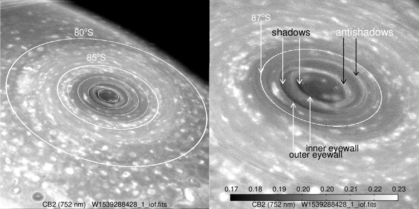
Figure 1.— Normal (left) and enlarged (right) views of Saturn’s south pole as captured in an ISS image taken with a CB2 (752 nm) filter on 11 October 2006. Planetocentric latitude lines are shown in the left panel for 80^∘S, and at 1^∘intervals from 85^∘S to 89^∘S. Sunlight was incident from the lower left when this image was taken. Cloud boundaries near 89^∘S and 88^∘S are the features commonly described as inner and outer eyewalls respectively. The features we define to be antishadows are indicated in the right panel.

The evidence that the dark crescents in the eye region are in fact shadows comes from their orientation relative to the direction of incoming sunlight. As the planet rotates, the shadows move in step with the longitude of the sun, as illustrated in Fig. 2, where incoming sunlight is shown by white arrows and black arrows point towards the Cassini spacecraft. Note also the bright antishadow associated with the outer “eyewall” moves with the sun as well, staying on the opposite side of the pole from the sun, and replacing the poleward shadow seen at the left in the first panel with an anti-poleward antishadow near the top of the third panel. The bright cloud feature just above the antishadow in the third panel (encircled by a large circle in each subpanel of Fig. 2) has only moved only about 30^∘ of longitude between the first and third panels, while the encircled smaller bright feature near the inner “eyewall” has moved about 80^∘ over the same interval. That feature also has moved more in longitude than the other features inside the inner eye and appears to be near the peak inner vortex angular motion profile measured by Dyudina et al. (2009) and Antuñano et al. (2015). Also note the elongated oval shape of the inner eyewall. Both of these inner eyewall features are also moving faster than bright features outside the eye region.

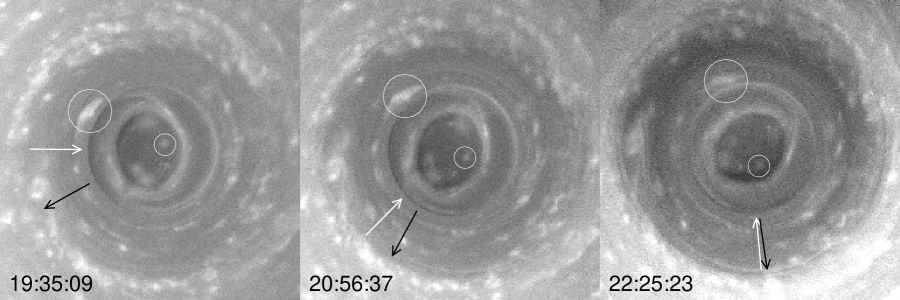
Figure 2.— Polar projections of a sequence of ISS 752-nm images of Saturn’s south polar region on 11 October 2006. Note that shadows follow the direction of incident sunlight, indicated by the white arrow in each panel. The black arrows point toward the Cassini spacecraft. The latitude circle tangent to the boundaries of each image has a radius of 5^∘ planetocentric. The zero of longitude is at the right.

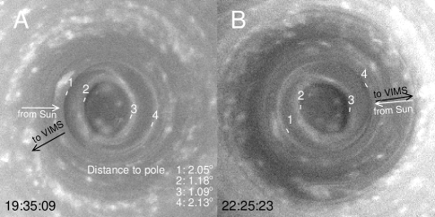
Figure 3.— Close-up view of first (A) and last (B) polar projections from Fig. 2. The putative eyewalls are marked by short white arcs labeled 1-4. These are located at longitudes 200^∘E (1 and 2) and 20^∘E (3 and 4) in A, but in panel B are shifted 40^∘E (1 and 4) and 73^∘E (2 and 3) due to zonal motions. The B image is shown rotated counterclockwise 90^∘ from its position in Fig. 2 to put the cloud features in roughly the same orientation as in A, at a time when the sun is incident from roughly the opposite direction. Note in particular the effects of sun reversal at boundary 3, which in A displays a relatively bright antishadow to its right with sunlight incident from the left, but in B, the antishadow disappears and the same edge casts a shadow to the left resulting from sunlight here coming from the right. If the shadow had been cast by a wall, that wall should appear to VIMS as a bright feature in A, extending to the left, opposite to what is observed.

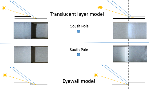
Figure 4.— Photographs of tracing-paper physical models illustrating two alternative shadow production mechanisms: a sharp change in optical depth of a translucent layer (top) or a step change in cloud pressure at an eyewall edge (bottom). Light from the sun is indicated by yellow rays, and light to the observer is indicated by blue rays. Each model produces a shadow on the lower layer when the transition is located on the sun-ward side (left) of the pole. But on the opposite side (right) the translucent layer model displays a moderately bright “antishadow” produced by light shining underneath the top layer and providing extra illumination from below, while the alternate model displays a brightly illuminated eyewall. When illuminated and observed at the angles illustrated here, which are comparable to those for the ISS images in Fig. 2, the antishadow is seen to extend from the upper layer boundary (marked by dashed lines) away from the pole, which is also the direction seen in the ISS images, while the bright eyewall is seen to extend towards the pole, in conflict with ISS observations. Figure from Sromovsky et al. (2019).

The behavior of shadows and antishadows is easier to see in an enlarged direct comparison between earliest and latest observations, as shown in Fig. 3. In this case the third panel of Fig. 2 is rotated 90^∘ counterclockwise to put the incident sun direction in that panel almost exactly opposite to that shown in the first image, while roughly retaining the same orientation of cloud features. Here, the solar elevation is near 25^∘, while the observer (VIMS) elevation angle is near 56^∘, which makes it possible to see whatever shadows are created, if dark enough and long enough. Shadow boundaries, marked by short arcs, appear in both images at the same cloud feature locations in both images (they track the zonal flow). When these boundaries are between the pole and the sun, they cast shadows toward the pole, but when they are on the opposite side of the pole from the sun, they cast antishadows away from the pole. If the shadows had been cast by vertical wall clouds, then in the opposite sun direction the walls would have been visible as bright features extending towards the pole.

The distinction between these two alternate shadow-producing mechanisms is perhaps more easily appreciated with photographs of a toy physical model presented in Fig. 4. At the top are photographs of a translucent separated layer model, constructed of tracing paper and shown in cross section above or below the corresponding photographs. The model was photographed in two different positions, corresponding to locations on opposite sides of a model pole. The incident sunlight is indicated by yellow rays and the blue rays point to the observer (VIMS). The sun and observer angles are comparable to those of the VIMS observations in Fig. 3. On the left a shadow is produced by the top layer of tracing paper, beginning where its optical depth drops to zero. On the right, an antishadow is produced by sunlight shining underneath the edge of the upper layer resulting in extra illumination from below, which is visible from above because the layer is not opaque.

For the eyewall model in Fig. 4, a shadow is produced when the wall is on the left, but on the right, the illuminated eyewall is visible to the observer and appears to extend towards the pole from the top boundary of the wall. The wall is much brighter than the top or bottom surfaces because they are illuminated at a low elevation, while the wall is illuminated at nearly normal incidence. This effect is also seen for hurricane eyewalls on Earth under similar observing conditions as we later illustrate in Sec. 5.1, along with Monte Carlo calculations showing similar results.

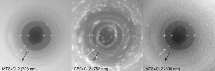
Figure 5.— Comparison of methane band images (MT2 at left and MT3 at right) and continuum ISS image (center) of Saturn’s south polar region on 11 October 2006, presented as a polar projection extending $\pm$5^∘ from the pole. The central ISS image was taken at 20:56:37.0 UT using a CB2 (752 nm) filter, and has an image scale of 16.8 km/pixel at the center of the image. Its identification number is W1539293315. The other images were taken 37 seconds earlier (890 nm image) and 37 seconds later (728 nm). The direction of incoming sunlight is indicated by white arrows and the direction of light traveling to the Cassini spacecraft is indicated by black arrows. Fiducial marks at the same set of locations in each image show that boundaries in the methane band images correlate with shadow and antishadow features in the continuum images. These cloud boundaries have come to be thought of as inner and outer eyewalls.

2.2. The evidence for deep convection

The evidence cited by Dyudina et al. (2009) for the deep convection over two scale heights, reaching higher than the tropopause, is the visibility of the eyewall clouds in methane band images. Although they did not display and annotate the relevant images in their paper, it seems clear that it is the boundaries displayed in Fig. 5 that form the basis for their inference. This figure displays polar projections of ISS images taken with methane band filters MT2 (728 nm) and MT3 (890 nm), in comparison with a polar projection of an image taken with the CB2 (752 nm) filter. The depth of penetration of these images can be roughly assessed from Fig. 6. At vertical viewing the two-way optical depth in the MT2 and MT3 filters are reached at pressure of 250 mbar and about 60 mbar respectively, the latter reaching above the tropopause ($\sim$70 mbar) even without accounting for the low view angle for the observations in question, which would lower these pressures by about a factor 3.1 ($\mu_{0}$ = 0.25, $\mu=0.5$). The CB2 filter on the other hand, reaches 2-way absorption optical depth unity at about 2.3 bars for the same observing and illumination geometry.

Fiducial marks on each image in Fig. 5 are placed at the same locations in latitude and longitude. The methane band images both show what appears to be a stair-step decrease in I/F towards the pole, with step changes occurring at the same locations as the boundaries associated with cloud shadows seen the the CB2 image in the middle panel. Neither methane band image actually shows either of the bright rings that might be associated with the top of an isolated eyewall. But in a hurricane seen from above, there is a thick cirrus outflow that blocks our view of the wall clouds. If that is happening in the polar region of Saturn, one would expect to see optically thick clouds extending somewhat away from the pole starting at each of the two boundaries. One would expect the composition of that “cirrus shield” to be the same as that of the deep convective cloud, which, if the Great Storm analysis is taken as a guide, might contain a mix of ammonia ice, water, and perhaps NH₄SH (Sromovsky et al. 2013), or even P₂H₄. But there is no evident 3-$\mu$m absorption that would indicate the presence of either NH₃ or NH₄SH. On the other hand, it is conceivable that the boundaries seen in the methane image are actually due to the changing character of upper cloud layers, which is not connected to deep convection at all, but is instead the cause of the cloud shadows from which the deep convection has been inferred.

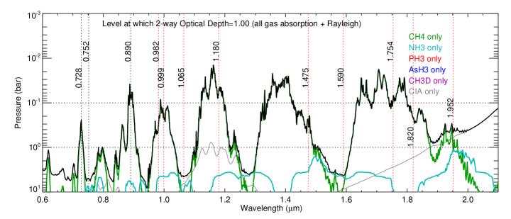
Figure 6.— Vertical penetration depth profile for wavelengths from 0.6 $\mu$m to 2.2 $\mu$m. Central wavelengths for ISS filters are located by vertical dotted lines. VIMS wavelengths spanning a similar range of penetration depths are indicated by vertical red dotted lines.

2.3. Possible radiative transfer constraints

There are two sorts of constraints that can further guide our interpretation of these features. One is the analysis of near-IR spectra in the south polar region to constrain the vertical cloud structure. Such an analysis might reveal the presence of optically thick clouds extending to high altitudes, or define the locations of layers on which shadows might be cast, or define changes in layer scattering properties with latitude, to see if the sudden disappearance of one layer at key latitudes could produce a shadow on a lower layer. There were in fact near-IR observations by the Visual and Infrared Mapping Spectrometer (VIMS) taken during the same period covered by the ISS images, and an analysis by Sromovsky et al. (2019) provides useful constraints on the models. While useful, these constraints are unable to be applied within shadows or close to shadow or antishadow boundaries, because they rely on the existence of horizontally homogeneous conditions. Thus they need to be supplemented by a radiative transfer analysis that can model conditions at and near such boundaries. For that we use Monte Carlo calculations. But these are limited in a different way. Because of the time involved in computing ray paths and interactions for many millions of photons, it is not practical to include the complexities of gas absorption models. Thus Monte Carlo calculations are mainly useful only for continuum spectral regions and pressure ranges, where gas absorption can be largely ignored. First, we consider the results of the VIMS analysis.

3. Vertical cloud structure inferred from Cassini VIMS

3.1. Overview of Cassini VIMS Near-IR results

The VIMS instrument (Brown et al. 2004) combines two mapping spectrometers, one covering the 0.35-1.0 $\mu$m spectral range, and the second covering an overlapping near-IR range of 0.85-5.12 $\mu$m. The near-IR spectrometer use 256 contiguous channels sampling the spectrum at intervals of approximately 0.016 $\mu$m. The near-IR VIMS spectra are particularly useful in constraining the composition of Saturn’s cloud layer because many of the candidate cloud materials have near-infrared absorption features, especially in the vicinity of 3 $\mu$m. From several studies of VIMS spectra in different regions on Saturn, including the Great Storm of 2010-2011 (Sromovsky et al. 2013) and its wake region (Sromovsky et al. 2016), the Storm Alley region (Baines et al. 2009a; Sromovsky et al. 2018), the north polar region (Baines et al. 2018), and the south polar region (Sromovsky et al. 2019), the following picture of Saturn’s multi-layer cloud structure has emerged.

Below a generally thin stratospheric haze, Saturn is covered by a thick cloud layer of unknown composition. This material seems to have no near-IR absorption features, although it may have features that are located within, and masked by, gas absorption features due to phosphine and ammonia. The prime candidate for this layer of particles is diphosphine. But we cannot test this hypothesis with spectral observations because the optical properties of diphosphine have not yet been quantitatively characterized. Another candidate that is far less likely on photochemical grounds is some form of white phosphorus. Lacking a dipole moment, a lack of significant near-IR absorption features would be expected for phosphorus.

Below this tropospheric mystery layer is a more well established layer of condensed ammonia. This material can be observed spectrally, but over most of Saturn its 3-$\mu$m spectral features can only be seen in areas of intense convection, such as in Storm Alley, or in the Great Storm of 2010-2011. Another place where the spectral features of NH₃ ice can be seen is in polar regions where the main upper tropospheric mystery cloud has dramatically reduced optical depth.

The deepest layer that can be sensed using visible to near-IR wavelengths is likely composed of NH₄SH. Where convection is vigorous, e.g., where lightning is observed, water ice may also be a significant cloud component. The deep clouds need to provide significant optical depth at pressures less than 5 bars in order to modulate the level of 5-micron emission observed on Saturn. If assumed to be optically dense, cloud top pressures in the 2-4 bar range are often found. Ammonia clouds could also modulate this emission to some degree, but in most cases the ammonia layer, as constrained by scattered sunlight observations, is too optically thin to provide much blocking of thermal emissions in the 4.8-5.1 $\mu$m region.

Radio observations have shown that lightning on Saturn has been highly variable over time, but highly localized in space. Lightning has only been observed in the Great Storm of 2010-2011, and in Storm Alley. No lightning has been observed in the south polar region, which makes it unlikely that there is any vigorous convection, even within the cloud structures identified as eyewalls.

3.2. Near-IR results for south polar vertical cloud structure

The Cassini Visual and Infrared Mapping Spectrometer (VIMS) also observed Saturn’s south polar region in 2006. Polar projections at selected wavelengths are displayed in Fig. 7. At the continuum wavelength of 1.065 $\mu$m, which is similar in penetration depth and appearance to images taken with the ISS CB2 (752 nm) filter but at an order of magnitude worse spatial resolution, we see clear shadow and antishadow features, with somewhat muted versions seen in the continuum wavelength of 1.59 $\mu$m. Lowered contrast for both features at longer wavelengths would be expected if they are produced by an optically thin overlying layer of small particles, because optical depths would decrease with wavelength. Eyewall clouds, on the other hand, would not exhibit much wavelength dependence because of their significant optical depths.

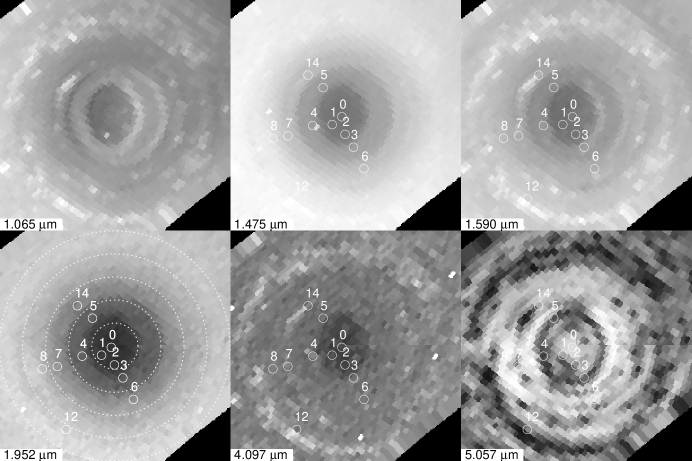
Figure 7.— VIMS images of the south pole of Saturn at six wavelengths indicated in the panel legends. These images (from cube V1539288419_1), were taken at 19:35:01 UT on 11 October 2006 at a phase angle of 37.2^∘ and with a sub-spacecraft pixel size of 145 km. Processing and calibration details are described by Sromovsky et al. (2019). The penetration depths of the wavelengths less than 2.2 $\mu$m are indicated by 2-way optical depth profiles in Fig. 6. The clear-atmosphere penetration depths at 4.1 $\mu$m and 5.06 $\mu$m are given by Sromovsky et al. (2019) and are about 1 and 3 bars respectively, which is where the two-way optical depth at normal viewing reaches unity. Numbered circles indicate the locations where complete near-IR spectra were analyzed by Sromovsky et al. (2019), with results plotted in Fig. 8. These polar projections provide complete coverage out to latitude 85^∘S, with latitude circles at 1^∘ intervals in the 1.952-$\mu$m image.

Sromovsky et al. (2019) derived model cloud structures at locations marked by numbered circles in Fig. 7 from the same VIMS observations (but using complete near-IR spectra, not just sample wavelengths). Note that these samples avoid small discrete cloud features and mostly stay away from shadow and antishadow boundaries. The results from their radiative transfer modeling of these background cloud spectra are plotted in Fig. 8. Unlike the dramatic reduction in optical depths found by Baines et al. (2018) within the eye of the north polar vortex, the changes seen as the south pole is approached are relatively modest. All four layers are preserved, but the stratospheric and putative diphosphine layers declined towards the poles, as might be expected in the case of downwelling motion. It is noteworthy that the NH₃ layer optical depth remained relatively constant for the background cloud structure, and none of the layers became completely cleared out within the eye region.

The top of the deep putative NH₄SH + H₂O layer varies between 3 and 4 bars, exhibiting more spatial structure than evident in the overlying layers. From 86.2^∘S to 89.8^∘S, the ammonia layer pressure smoothly decreases from about 1 bar to 800 mbar, and its optical depth (at 752 nm) appears to be constant over that range, at a value of 0.615, but with a substantial uncertainty of about 25% in individual fit results. The putative P₂H₄ layer moves slightly downward as the pole is approached, from about 300 mbar to 430 mbar, while its optical depth declines from about 0.39 to 0.27, likely occurring mostly in a step decrease of 0.12 at 88.9^∘N, the location of which is based on ISS images. The effective pressure of the stratospheric haze decreases then increases as the pole is approached, with a log slope vs latitude comparable to that seen in the putative P₂H₄ layer. Its optical depth decreases toward the pole, most likely occurring mainly in a step change from 0.39 to 0.24 at 87.9^∘S. The particle radii for the stratosphere and putative P₂H₄ layers average about 0.18 $\mu$m and 0.6 $\mu$m respectively, with very little change versus latitude. The ammonia layer particle radius declines from about 1.9 $\mu$m to 1.1 $\mu$m as the pole is approached.

The upper two layers dip downward in altitude near the pole, while the ammonia layer rises upward slightly, suggesting that the polar downwelling is limited to the upper two layers. It also appears that the upper two layers are plausible sources of shadows on the ammonia layer, and perhaps to some degree on the deeper layer. Whether the optical depth declines in the stratospheric haze and in the putative diphosphine layer (upper tropospheric layer) are smooth functions of latitude or in the form of sudden step changes could not by determined from the radiative transfer modeling of VIMS spectra, both because the model assumption of horizontally homogeneous conditions do not apply at the transitions, and, even if they did, the uncertainty in retrieved parameter values is large enough to obscure the transition details. However, Sromovsky et al. (2019) did conclude that the transitions were in the form of step changes at in the stratospheric haze and P₂H₄ layers because images sensing those layers predominantly (mainly using the MT2 filter) did show step changes in I/F, as is evident in our Fig. 5, and in the VIMS images at 1.475 $\mu$m and 1.952 $\mu$m, which are shown in Fig. 7. While the VIMS spectral modeling results did not discover anything that might be considered evidence for deep convective eyewalls, they did provide evidence for declining optical depth and, with the help of imaging observations, evidence that the decline is almost certainly in steps.

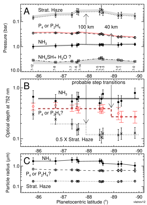
Figure 8.— Best-fit parameter values vs. latitude for cloud structure fits to background cloud spectra between 85.8^∘S and the south pole, including pressures (A), optical depths at 752 nm (B), and particle size (C). The solid gray horizontal bar in (B) is at optical depth 0.615, the dashed step is from 0.39 to 0.27 optical depths at 1.1^∘from the pole, and the dotted step is from 0.39 to 0.24 optical depths at 2.1^∘from the pole, but plotted at half scale to eliminate overlap with the upper layer. From Sromovsky et al. (2019).

In the following, we will show that step changes in optical depth of a translucent overlying layer can produce shadows on a lower layer and antishadows visible at the top of the shadow casting layer. We will also show that if eyewalls were present they would indeed create bright features that would replace shadows as the sun’s direction reversed, but the location of those bright features is in conflict with observations. We begin with a description of our Monte Carlo calculation methods.

4. Monte Carlo radiative transfer methodology

4.1. Motivation and limitations

Our doubling and adding routines for radiative transfer assume that atmospheric gas and aerosol structures are horizontally homogeneous. Practically speaking, this means that the horizontal variation scale is much larger than the vertical scale. Since the vertical scale of the cloud structure is of the order of 100 km, and the horizontal variation with the eye region is of the same scale in many locations, and even smaller scales at shadow boundaries, we cannot use our normal methods to do accurate radiative transfer modeling in the vicinity of shadows. To model I/F profiles in the vicinity of cloud boundaries, we thus turned to Monte Carlo calculations, which can handle such situations. However, the time consuming nature of such calculations requires us to simplify the problem by working only at wavelengths for which atmospheric absorption can be neglected. At 752 nm, atmospheric absorption is minimal, reaching a vertical 2-way absorption optical depth of unity at about the 8-bar level. But at the typical slant angles of the subject observations, the zenith angle cosines are $\mu_{0}$ = 0.25 for illumination and $\mu$ = 0.55 for viewing, so that the absorption optical depth of unity is reached at p = 8 bar /(0.5/$\mu_{0}$ + 0.5/$\mu$), which evaluates to 2.3 bars. At the top of the NH₃ layer, which is near 800 mb, the two way absorption optical depth would only be about 0.35. The importance of this absorption would be amplified by reflections between layers, but this effect is not as important for optically thin layers that lose photons before many reflections can occur. To better assess the importance of ignoring atmospheric absorption in our Monte Carlo calculations, we ran a full radiative transfer model calculation for a background cloud feature at 88.6^∘S using parameters in column 5-3 of Table 4 of Sromovsky et al. (2019) and using the same radiative transfer code, then computed a spectrum for the same aerosol model but with the methane mixing ratio reduced by a factor of 10. This only produced a 10% increase in the I/F at 752 nm for the appropriate observing and illumination conditions. Thus, we are confident that our neglect of atmospheric absorption at 752 nm will not seriously impact our Monte Carlo calculations.

4.2. Vertical and horizontal structure model

Our basic aerosol structure model consists of a layer of finite (and adjustable) thickness defined by upper and lower boundaries $z_{1}$ and $z_{2}$, suspended at a height $z_{1}$ over a Lambertian scattering surface at $z=0$. The scattering layer is three dimensional, but its properties are invariant in the $x$ dimension. Our coordinate system and the simplified model are illustrated in Fig. 9. All properties are assumed invariant in the $x$ direction, but a discontinuity in suspended layer properties and surface reflectivity are allowed at $y$ = 0. For the suspended layer we assume that optical density, i.e., optical depth per unit length, is independent of altitude between $z_{1}$ and $z_{2}$, defined by the vertical optical depth $\tau$ divided by the layer thickness $(z_{2}-z_{1})$. For $y<$ 0 we assume $\tau=\tau_{1}$, single scattering albedo $\varpi=\varpi_{1}$, and a surface albedo $a_{1}$, while for $y>$ 0 we assume $\tau=\tau_{2}$, $\varpi=\varpi_{2}$, and surface albedo $a_{2}$. This allows for absorption by the aerosol particles and by the surface. The scattering and absorption by the atmosphere, as noted earlier, are ignored.

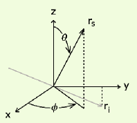
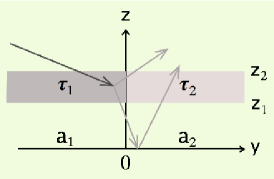
Figure 9.— Coordinate system for Monte Carlo calculations (left), where vector $r_{i}$ indicates a typical incident ray in the $y-z$ plane, and vertical structure model (right), shown in cross section, with a sample incident ray (in black) and a few possible scattered rays (in gray) following a random interaction sequence. For these examples the only scattering occurs in the layer between $z_{1}$ and $z_{2}$ or at the surface, both of which are uniform in the $x$ direction but can have different scattering properties for $y<0$ and $y\geq 0$. The $x$-$y$ positions of incident and exit rays are measured where they intersect the $z=z_{2}$ plane.

4.3. The Monte Carlo sampling equations

A key element of Monte Carlo radiative transfer is randomly sampling scattering parameters, some of which can have non-uniform probability distributions $P(x)$, such as optical depth and scattering angle. To do this with a random number generator that produces values uniformly distributed between 0 and 1, we make use of the cumulative probability distribution function, given by

$$P_{C}(x)=\int_{xmin}^{x}P(x^{\prime})dx^{\prime}/\int_{xmin}^{xmax}P(x^{\prime})dx^{\prime},$$ (2)

where $P_{C}(x)$ varies from 0 to 1 as $x$ ranges from $xmin$ to $xmax$. If $P_{C}$ is set equal to uniformly distributed random values between 0 and 1, and then inverted to find the corresponding values of $x$, it is easy to see that these $x$ values will be distributed in proportion to the slope $dP_{c}(x)/dx$ = $P(x)$, which provides the desired probability distribution of $x$. In some cases $P_{C}(x)$ can be computed analytically, while in others, it is necessary to compute numerical integrals to create a table of $x$ and $P_{C}(x)$ values. In either case a random value of $x$ is obtained by solving for $x$ in the equation

$$\xi=P_{C}(x)$$ (3)

where $\xi$ is selected randomly from a distribution that is uniform between 0 and 1. To sample optical depths between zero and infinity, we use

$$\tau=-\log_{e}(1-\xi)$$ (4)

To sample an azimuthal angle and zenith angle cosine from an isotropic scattering phase function, we use

$$\phi_{s}=2\pi\xi_{1}$$ (5)

$$\mu_{s}=2\xi_{2}-1$$ (6)

where the different subscripts on $\xi$ indicate that two unrelated random samples are chosen for the two directional parameters. For scattering according to a Henyey-Greenstein (HG) function, there is an analytical function for sampling the cosine of the scattering angle (Witt 1977), which is given by

$$\mu_{s}=\frac{1+g^{2}-[(1-g^{2}).(1-g+2g\xi)]^{2}}{2g}\quad\mathrm{for~{}}g\neq 0$$ (7)

$$\mu_{s}=1-2\xi\quad\mathrm{for~{}}g=0$$ (8)

However, for double H-G functions or Mie scattering we are reduced to interpolation of numerical tables to find the value of $\mu_{s}$ for a given sample of $\xi$. To facilitate tracing of the scattered ray, the direction specified by $\mu_{s}$, which is the cosine of the scattering angle, and $\phi_{s}$, which is an azimuth angle of the scattered ray measured in a plane perpendicular to the incident vector, must be expressed in terms of cosine $\mu$ and angle $\phi$ as defined in the original coordinate system.

4.4. The Monte Carlo ray tracing algorithm

Our basic approach is along the lines described by Whitney (2011). We choose a specific direction for incoming sunlight, specified by a zenith angle cosine $\mu_{0}$, and an azimuth angle $\phi_{0}$, which is the angle of the vector projection in the $x$-$y$ plane measured from the $x$ axis counter clockwise about the $z$ axis (Fig. 9). Because the incoming light from the sun is a downward vector in this coordinate system its zenith angle cosine $\mu_{0}$ is negative. In what follows, we only consider cases in which the incoming light is in the $y$-$z$ plane. Next, a random incident location uniformly distributed between $y=$-L and $y=$+L is chosen. Recall that y positions are measured at the top of the scattering layer (the $z=z_{2}$ plane). (Although the scattering layer is three dimensional and photons are scattered in three dimensions, because there is no variation of layer properties in the $x$ direction, we choose all incident rays to be incident at $x=0$ and ignore $x$ variation in the output results.) Our next step is to choose a random optical depth using Eq. 4. This optical depth is then converted to a physical distance over which the photon travels before interacting with a scattering particle or the surface. Inside the scattering layer we find a distance by dividing by the optical density (optical depth per unit length). If the length times $\mu_{o}$ exceeds the layer thickness, the photon will exit the bottom of the layer and hit the surface. Otherwise it will scatter inside the layer.

If the photon scatters inside the layer, then it either gets absorbed within the layer with a probability 1-$\varpi$, or it scatters in a random direction. If it is absorbed it will not be counted. If it scatters, the direction will be randomly chosen in accord with the assumed phase function, using the above sampling equations. If the particle passes through the upper layer and reaches the surface, it may be absorbed or reflected. If the surface albedo is less than 1, its probability of being reflected is equal to either $a_{1}$ or $a_{2}$, depending on whether it impacts the surface at $y<0$ or $y>0$. What happens to a specific photon is determined by taking a uniformly distributed sample $\xi$. If $\xi$ is less than 1-$a_{1}$, for example, then the photon is absorbed and that photon is not counted. Otherwise the photon is reflected, and then a random reflection direction is chosen, using $\phi=2\pi\xi_{1}$ and $\mu=\sqrt{\xi_{2}}$. The latter relation can be obtained from the constraint that the radiance of a Lambertian reflector is independent of observing angle.

Once a new location and direction are determined for the photon, a new optical depth is sampled, the photon path is traced to its next interaction, following the same procedures. The ray tracing is complicated by the fact that there are two different regions with different properties, i.e. for $y<0$ and $y\geq 0$ (see Fig. 9). If the photon is not absorbed, it will eventually exit the top of the scattering layer, at which point its exit location and direction will be saved for later binning and computation of radiance and I/F. The uncertainty of a binned value is taken to be the square root of the number of photons in the bin. For reasonable accuracy without excessive computer time we generally used between 20 and 100 million incident photons. Computation time for a given case ranged from 20 minutes to an hour or more.

4.5. Computing radiance and I/F from binned photon counts

For a given observer viewing geometry specified by $\phi_{v}$ and $\mu_{v}$, and chosen respective bin sizes $d\phi_{v}$ and $d\mu_{v}$, we find array locations for all the photons falling inside the viewing bins and then compute a histogram of all those photons as a function of spatial location $y$ at which photons are incident at the top of the scattering layer, computing their counts in bins of size $dy$. If $N_{phot}$ is the total number of photons that are incident, then the photon flux is the number of photons per unit area orthogonal to the incident direction, i.e. $F_{\mathrm{phot}}=N_{\mathrm{phot}}/(|\mu_{0}|(\Delta y\Delta x))$, where $N_{\mathrm{phot}}$ is the total number of photons that were incident (per unit time is implicit), $\Delta y=2L$, and $\Delta x$ is some arbitrary distance in the $x$ direction (all variation in the $x$ direction is ignored). The photon radiance for a Lambertian surface so illuminated is then given by $R_{\mathrm{Lambert}}=F_{\mathrm{phot}}/\pi$. The observed photon radiance is given by $R_{\mathrm{photon}}=dN_{\mathrm{phot}}(y,\mu_{v},\phi_{v})/(dy\Delta xd\mu_{v}d\phi_{v}\mu_{v})$, where $dN_{\mathrm{phot}}(y,\mu_{v},\phi_{v})$ is the number of photons in bins $y\pm dy/2$, $\mu_{v}\pm d\mu_{v}/2$, and $\phi_{v}\pm d\phi_{v}/2$. The reflectivity is then computed as I/F = photon radiance/Lambert radiance, in which the arbitrary interval $\Delta x$ cancels out:

$$I/F=\pi\>|\mu_{0}|\>\times$$

$$dN_{\mathrm{phot}}(y,\mu_{v},\phi_{v})/[N_{\mathrm{phot}}\mu_{v}d\mu_{v}d\phi_{v}dy/\Delta y].$$ (9)

4.6. Code validation

The code used for the Monte Carlo calculations was tested first by setting model parameters on both sides of the boundary to the same values and then comparing those results with doubling and adding computations for the same vertical structure and particle scattering parameters. We next used different parameter sets for the two regions of the Monte Carlo code and verified that away from the joint the Monte Carlo results approached the values obtained for horizontally uniform conditions. Although we could not directly verify radiance calculations near the discontinuity in parameter values (i.e. at and near $y=0$), we did verify that the ray tracing was being done correctly, by following rays as they crossed into different regions to verify that correct branches were chosen in the computation of scattering probabilities and directions. Finally, as a sanity check, we built a physical model that generated shadows and antishadows, and were able to produce similar effects with the Monte Carlo code.

5. Monte Carlo calculation results

5.1. Scattering properties of eyewalls

The term eyewall we take to imply optically thick vertical convective towers similar to what is observed in hurricanes on Earth. If not heavily obscured by cirrus outflow clouds, eyewalls would be able to cast shadows on either side of the pole, both when the sun was incident toward the pole and when it was incident away from the pole. As shadows on Saturn are only observed to extend toward the pole, either the eyewalls are obscured by cirrus outflow, or they do not exist. Another property of earthly eyewalls is that when illuminated at low sun angles, they are very bright in comparison to the top visible cloud layer, which becomes dark as the sun sets. If we approximate both the top and wall clouds as Lambertian reflectors of unit albedo, the brightness of the top would be proportional to $\mu_{0}=\cos{\theta_{0}}$, while that of the wall would be proportional to $\sin{\theta_{0}}$, so the ratio of the wall I/F to the top I/F is roughly proportional to the tangent of the solar zenith angle, yielding a ratio of 3.9 to 1 at $\theta_{0}$ = 75.5^∘. An example of this effect can be seen in the left panel of Fig. 10, which displays the eye of hurricane Irma at a low sun angle. A scan through the center of the eye, shows that the shadow is very deep, only about 10% of the brightness of clouds outside the wall, while the illuminated eyewall is about double the brightness of background clouds.

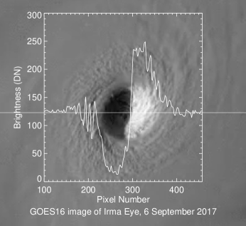
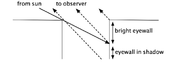
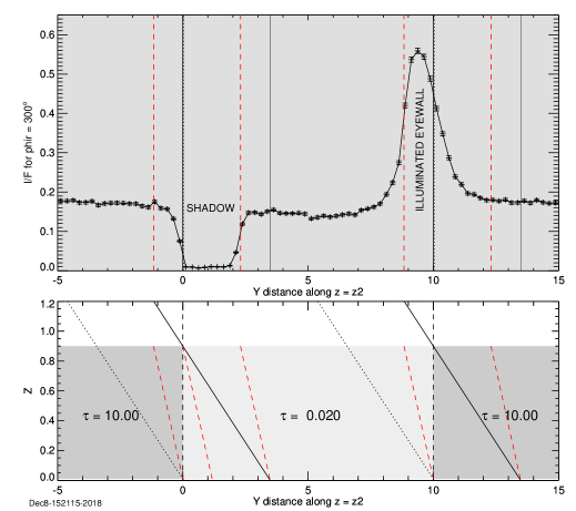
Figure 10.— Left: The eye of hurricane Irma at low sun angles displays an illuminated eyewall that is much brighter than the top cloud layer of the hurricane. The illumination and observing geometry is shown below the image and a scan across the circular eye displays the brightness profile. Right:. A similar brightness profile is seen in Monte Carlo calculations for Saturn’s south polar region under 2006 Cassini observing conditions. This calculation is for an eye with a width much greater than its height, so that the shadow does not fall on the eyewall. The diagram in the lower part of the right panel displays incoming solar rays with black lines and observer sight lines with dashed red lines. The wall clouds have a vertical thickness of 0.9 units of distance and a separation of 10 units. The illumination is at $\mu_{0}=-0.25$ and the sight line is at $\mu_{v}$ = 0.55, with $\phi_{0}=90$^∘ and $\phi_{v}=270$^∘. The observer is thus able to see the eyewall shadow on the left and the illuminated eyewall on the right. The I/F profile across this structure is shown in the top panel, computed for conservative cloud particles of radius 5-$\mu$m, refractive index of 1.82+0$i$, and vertical optical depth of 10. At the bottom of the model we assumed a Lambertian surface of albedo = 0.6

A Monte Carlo calculation for a typical south polar Saturn viewing geometry is shown in the right panel of Fig. 10. Note that the I/F at the top of the wall, away from the eye region is about 0.18, while in the shadow it is near zero and in the illuminated eyewall it peaks near 0.55, which is about 3.1 times the background I/F (a little below the ratio of 3.9 given by the Lambertian approximation described in the previous paragraph). The peak - background difference of 0.37 is 2.2 times the background - shadow difference of 0.17. Redoing the calculation with a particle radius of 0.5 $\mu$m instead of 5.0 $\mu$m, yielded a slightly larger peak and slightly larger background, but a similarly large difference ratio, in this case 2.45 instead of 2.2. Particle radii between 0.5 and 5 $\mu$m gave intermediate results. Reducing the optical depth of the eyewall clouds by a factor of five reduced the peak I/F to 0.35 (for a 1-$\mu$m particle), which is still almost twice the background I/F of 0.18, although the differential difference ratio dropped to about 1.0. Yet, the location of the peak is still inside the eye, rather than on the top of the wall cloud. It should be noted that an optical depth of 2.0 is too low to be considered characteristic of a deep convective eyewall.

5.2. Scattering properties of translucent layers

It is also possible for optical depth changes in a translucent upper aerosol layer to create shadows on an underlying layer, and to also create bright features under appropriate illumination conditions. This is illustrated by a physical model displayed in Fig. 11. The shadow is darker than both the covered and uncovered regions away from the shadow because it is missing both direct sunlight and the extra scattered light provided by the upper layer. In the bright region, in the right half of the panel, light is able to provide extra illumination underneath the top layer which increases its brightness above its normal value, seen further from the edge, where there is no extra illumination. Note that the bright region, which we call an antishadow, has a width that is essentially the same as that of the shadow in this case, and appears to be a general feature of most of our trial calculations.

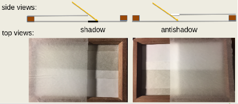
Figure 11.— A physical model illustrating the creation of shadows and antishadows by a translucent layer overlying a deeper scattering layer. Here a wooden frame is used to suspend a sheet of tracing paper a short distance above several overlapping sheets that produce underlying albedo structure, which is visible through the overlying layer. Only part of the deeper layer is covered by the suspended sheet. In both views light is incident at a low angle from the left. On the left, the upper sheet covers about the left 60% of the bottom sheets, while on the right it covers the right 60%. The result on the left is a shadow and, on the right, a bright region of similar width, which we call an antishadow.

To determine how shadow depth and antishadow brightness depend on the optical depth difference between two sides of an upper translucent layer, we make use of the simplified Monte Carlo model described previously. Fig. 12 displays the results of Monte Carlo calculations for a physically thin layer above a Lambertian reflector. The upper layer has a transition from $\tau_{1}$ to $\tau_{2}$ at y = 0 and back to $\tau_{1}$ at y=10. We show two examples. Both have $\tau_{1}$ = 0.5. The first case, which is most similar to the physical model, has the most dramatic transition, to $\tau_{2}$ = 0.01 and back. In the second case the transition is to $\tau_{2}$ = 0.25 and back. The vertical structure, shown in the bottom panel, has the upper scattering layer confined between z = 0.65 and z = 0.70, where distance along y and z have the same arbitrary scale. The more dramatic transition displays a deep shadow that has its lowest I/F displaced towards the outer limit of the shadow boundary as also seen in the physical model. The less dramatic transition produces flatter and shallower shadows and antishadows. The shapes of the shadow and antishadow features also vary with viewing geometry and with the thickness of the shadowing layer and its elevation above the lower Lambertian reflecting layer. Both features are also widened if the transition itself occurs smoothly over a short distance rather than as a step change. However, detailed computations for gradual transitions are much more complex to model and beyond the capabilities of our current code.

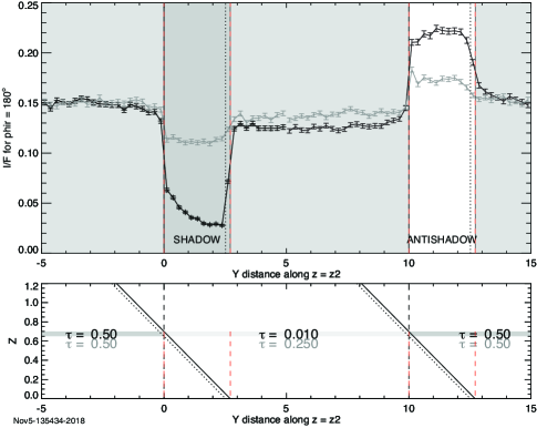
Figure 12.— Monte Carlo I/F calculation for a physically thin layer with step changes in opacity, above a Lambertian reflecting layer of albedo 0.5. The incident light is coming from the left at $\mu_{0}$ = -0.25 at azimuth 90^∘ (in the y-z plane). The observer is at $\mu$= 0.55, with azimuth 180^∘(in the x-z plane). The layer structure and observing and illumination geometry are illustrated in the bottom part of the figure, with the I/F profile in the upper portion. The particles in the layer are assumed to scatter conservatively with an HG phase function of asymmetry $g$ = 0.5 to simulate slightly forward scattering particles. The shadow boundary is at $y=0$, while the antishadow boundary is at $y=10$. The distance scale is relative, but the same in $z$ and $y$ directions. Slanted solid and dotted lines in the bottom panel indicate incident rays, while dashed red lines indicate the projections of observer sight lines onto the y-z plane.

5.3. Quantitative comparisons with observed I/F profiles

Monte Carlo calculations for optical depth step changes of 0.05 to 0.1 from a base level of 0.35 to 0.5 were found to produce I/F amplitudes of about 10%, which is about the right amplitude to match the I/F variation seen at 752 nm. We also found that if we used similar transitions in the optical depth of the diphosphine layer (near 250 mbar), we could match the I/F changes of 15% to 20% seen at 728 nm, which is most sensitive to that layer. Direct comparisons between I/F scans and Monte Carlo model transitions are shown in Fig. 13. The absorption at 728 nm was not included in the Monte Carlo calculation directly. Instead we assumed that there was no contribution from below that layer due to that attenuation, then just scaled the Monte Carlo I/F to account for absorption of incoming and outgoing light by the methane above the layer.

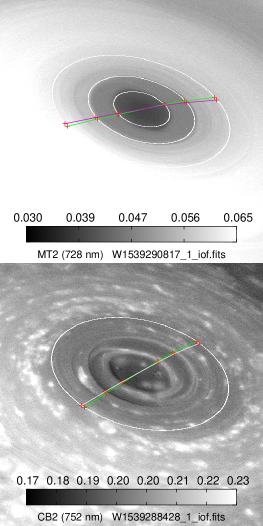
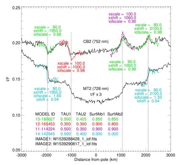
Figure 13.— Comparison of observed I/F profiles along lines indicated in images in the left two panels with Monte Carlo model profiles at and near boundaries where step changes in optical depth occur. The blue models are compared to the 728-nm I/F profile after multiplying the model length scale by the factor $xscale$ and boosting the I/F by the factor $yscale$. The $xshift$ parameter controls the horizontal position of the model I/F boundary and is adjusted to match the location of the observed I/F step. The I/F scale changes are equivalent to the same fractional adjustments needed in the size of the optical depth steps.

The shadow calculations shown in Fig. 13 were done in the relative scale domain. The physical scale estimate was made by finding a multiplication factor in km that produced approximately the correct width of the calculated features. With our cloud tops at 0.9 relative units and scale factors of typically 90 to 100, this led to rather large distances between the shadowed layer and the shadow-casting layer, of typically 80-90 km. That is more altitude separation than the 60-70 km that exists between the stratosphere and diphosphine layers, but less than the altitude separation between the stratosphere and the NH₃ layer. Given the semi-transparent nature of the P₂H₄ layer, is is conceivable that the observed shadow is actually a combination of shadows on both layers. Unfortunately, our Monte Carlo code is too simple to handle the shadowing of one layer onto two lower layers.

More problematic is the situation for the inner transition near 1.1^∘ from the pole. In this case the model needs a similar 80-90 km vertical separation between layers, but only about half that distance exists between the diphosphine layer with the transition and the underlying ammonia layer (see Fig. 8). However, the ammonia layer itself may be sufficiently transparent that a shadow falling through the ammonia layer onto the deep layer might contribute to the observed length of the inner shadow. Even though its optical depth is about 0.6 at 752 nm, its larger particles will forward scatter, so that they will be more translucent that might be initially expected. The deeper layer is of the order of 100 km below the diphosphine layer.

6. Evaluation of shadow and antishadow possibilities

Six different shadow-generating vertical cloud profiles are plotted in Fig. 14. We consider each of these cases and weigh the evidence that is relevant.

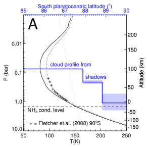
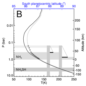
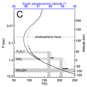
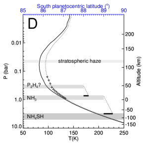
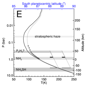
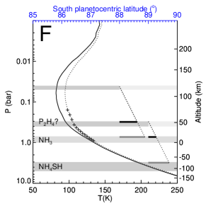
Figure 14.— Six candidate cloud profiles that might be at least crudely consistent with shadow measurements by Dyudina et al. (2009). Panel A starts with an outer cloud at the tropopause level, which must be 30 km above the cloud level on which it casts shadows, and that layer is assumed to cast shadows on a layer that is roughly 70 km deeper, which would put it near the 1 bar level. Examples B and C contain deeply convective “eyewall” clouds that cast shadows on the NH₃ layer, or first on the NH₃ layer and then on the NH₄SH layer. In panel D, the shadows are cast by upper layers on lower layers without deeply convective wall clouds. In panel E, the step changes in the optical depth of the putative diphosphine layer casts both inner and outer shadows on the ammonia layer, and in panel F, an optical depth step in the stratospheric haze casts a shadow on diphosphine and ammonia layers and a step change in the diphosphine layer casts a shadow on the ammonia and NH₄SH layers.

Panel A (stair steps of optically thick clouds). This starts with clouds tops reaching above the tropopause, declining about 30 km near 88^∘S, then declining another 70$\pm$30 km near 89^∘S, with no overlying cloud layers. This can be rejected because VIMS spectral constraints do not find optically thick clouds or any significant pressure changes in any of the four cloud layers, and especially no layers in which clouds are completely cleared out. Also, there are no observations of bright eyewalls that should be produced by such a structure, and no mechanism to create antishadows that are observed. Furthermore, the shadows from such structures would be very dark, not just 10% perturbations of the I/F profile with latitude.

Panel B (two deep convective eyewall clouds casting shadows on a background ammonia layer). In this case different shadow lengths arise from different heights of inner and outer wall clouds. A thick cirrus outflow away from the pole must be rejected because it would obscure the shadow from the outer eyewall. But for a thin outflow layer, shadows should be seen on both sides of the pole, unless the eyewalls have a shallow slope extending a long distance away from the pole. But VIMS constraints indicate that all layers slope downward toward the pole instead of away from it. Also, there is no evidence in the spectra for deeply convective optically thick clouds, as well as no observations of lightning that might be expected from such convection, as seen elsewhere on Saturn. Further, this structure provides no mechanism for producing antishadows.

Panel C (two deep convective eyewalls casting shadows on different layers). In this case the inner eyewall casts a shadow on the putative NH₄SH layer and generates an ammonia ice outflow layer on which the outer eyewall casts its shadows. If the outflow layers are thick, this would prevent forming the second set of shadows on the side of the pole opposite where poleward shadows are created. But these should produce bright eyewalls, which are not seen, and cannot produce antishadows, which are seen. Also, VIMS spectra provide no evidence for optically thick clouds in this region, and also no clear regions interior to the shadow forming cloud boundaries.

Panel D (P₂H₄ layer casting outer shadow on NH₃ layer which casts inner shadow on NH₄SH layer). In this case two cloud layers simply disappear in succession as a function of increasing latitude (toward the pole). The top layer would then cast a shadow on the next layer down, and finally the second layer would cast a shadow on the third layer. This has the virtue of providing height differentials that are consistent with shadow length measurements of Dyudina et al. (2009), and is also capable of producing both shadows and antishadows. But the successive clearing of upper layers is inconsistent with VIMS spectral results, and the large optical depth changes by clearing transitions would produce much deeper shadows and brighter antishadows than are observed.

Panel E (the P₂H₄ layer produces both inner and outer shadows on the NH₃ layer by step changes in optical depth). This was the model that seemed most consistent with our initial VIMS analysis (Sromovsky and Fry 2018) for which the stratospheric haze was forced to be at too low a pressure. Our current analysis indicates that the stratospheric haze has a more significant optical depth and is likely the location of the outer step in optical depth, with the putative P₂H₄ layer being the most probable location of the inner optical depth transition. This structure also is problematic in having too little distance between layers that create the inner shadow, requiring that the shadow length be extended perhaps by an attenuated shadow on the deeper layer. A quantitative evaluation of this of this multi-layer shadow is beyond the capabilities of our current Monte Carlo code.

Panel F (a step change in the stratospheric haze optical depth casts a shadow primarily on the P₂H₄ layer, and a similar optical depth step in the putative P₂H₄ casts a shadow primarily on the NH₃ layer, but also on the deeper putative NH₄SH layer). This has the best consistency with VIMS spectra, and at least the outer transition is supported by our Monte Carlo calculations, but the inner model shadow on the NH₃ layer is too short to fit the observations. The longer shadow that might fall on the deeper layer might produce a better match to the observations, but our Monte Carlo model is insufficiently complex to treat the combination of all three layers, and reach a definitive conclusion about the inner shadow.

The weight of the evidence favors the production of shadows by relatively sharp optical depth transitions with latitude, the outermost being in the stratospheric haze layer and the innermost being in the putative diphosphine layer. This mechanism can produce both shadows and antishadows of approximately the correct amplitude, and does not require deep convective clouds that are not observed, and thus the lack of lightning detections is also consistent with this structure.

7. Summary and Conclusions

Our analysis of Cassini/VIMS spectra of the south polar region of Saturn have led to the following conclusions.

1. The cloud structures inferred from radiative transfer modeling are not consistent with the step change in cloud altitudes derived from cloud shadows by Dyudina et al. (2009). None of the modeled cloud layers disappear, and their optical depths are relatively small and do not change dramatically with latitude. There is no evidence for an optically thick vertical wall of clouds as found in hurricanes on Earth.

2. Monte Carlo calculations confirm that illuminated eyewall clouds should be very bright and that these bright features should appear to extend poleward from the wall boundary as would the shadows that such a wall would produce with the sun in the opposite direction. But this contradicts the finding of slightly bright features extending away from the pole (Fig. 3), which is the expected direction for antishadows.

3. The shadow boundaries do correlate with changes in scattering properties of overlying hazes, which appear to involve two step changes in optical depth, one in the stratospheric haze near 2.1^∘ from the south pole, and one in the putative diphosphine haze near 1.1^∘ from the pole. According to Monte Carlo calculations, these steps are of sufficient magnitude to produce weak shadows, and weak shadows are observed (Fig. 13).

4. The shadows produced by the overlying hazes have the appropriate physical configuration to explain the anti-shadows observed on the opposite side of the pole from the shadows. These are regions of local brightness increases produced by sunlight illuminating the layer underneath the shadow casting layer, causing it to appear brighter from above than the region further from the pole that does not receive that extra source of light.

There remain a number of questions to be resolved about these features. A better constraint on the cloud structure might be obtained from more complex Monte Carlo calculations that can handle more complex and more realistic vertical variations, including multi-layer shadows and anti-shadows. It would also be interesting to apply this analysis to the north polar region. It is curious that in spite of large decreases in optical depths of haze and cloud layers as the north pole is approached (Baines et al. 2018), prominent cloud shadows have not been noted at high north polar latitudes, perhaps because the layers on which those shadows might be cast are also of low optical depth or because the transitions are insufficiently sharp. That situation could benefit from further investigation. There also remain significant uncertainties regarding the composition of the ubiquitous upper tropospheric layer, which seems likely to be either diphosphine or some form of phosphorus. But to test which better fits the spectral observations, we need better measurements of the optical properties of both of these materials under Saturnian conditions, especially of diphosphine about which very little is known.

References

- Antuñano et al. (2015) Antuñano, A., Río-Gaztelurrutia, T., Sánchez-Lavega, A., Hueso, R., 2015. Dynamics of Saturn’s polar regions. J. of Geophys. Res. (Planets) 120, 155–176.
- Baines et al. (2009a) Baines, K. H., Delitsky, M. L., Momary, T. W., Brown, R. H., Buratti, B. J., Clark, R. N., Nicholson, P. D., 2009a. Storm clouds on Saturn: Lightning-induced chemistry and associated materials consistent with Cassini/VIMS spectra. Planet. & Space Sci.57, 1650–1658.
- Baines et al. (2009b) Baines, K. H., Momary, T. W., Fletcher, L. N., Showman, A. P., Roos-Serote, M., Brown, R. H., Buratti, B. J., Clark, R. N., Nicholson, P. D., 2009b. Saturn’s north polar cyclone and hexagon at depth revealed by Cassini/VIMS. Planet. & Space Sci.57, 1671–1681.
- Baines et al. (2018) Baines, K. H., Sromovsky, L. A., Fry, P. M., Momary, T. W., Brown, R. H., Buratti, B. J., Clark, R. N., Nicholson, P. D., Sotin, C., 2018. The Eye of Saturn’s North Polar Vortex: Unexpected Cloud Structures Observed at High Spatial Resolution by Cassini/VIMS. Geophys. Rev. Let.45, 5867–5875.
- Brown et al. (2004) Brown, R. H., Baines, K. H., Bellucci, G., Bibring, J.-P., Buratti, B. J., Capaccioni, F., Cerroni, P., Clark, R. N., Coradini, A., Cruikshank, D. P., Drossart, P., Formisano, V., Jaumann, R., Langevin, Y., Matson, D. L., McCord, T. B., Mennella, V., Miller, E., Nelson, R. M., Nicholson, P. D., Sicardy, B., Sotin, C., 2004. The Cassini Visual and Infrared Mapping Spectrometer (VIMS) Investigation. Space Sci. Rev. 115, 111–168.
- Dyudina et al. (2007) Dyudina, U. A., Ingersoll, A. P., Ewald, S. P., Porco, C. C., Fischer, G., Kurth, W., Desch, M., Del Genio, A., Barbara, J., Ferrier, J., 2007. Lightning storms on Saturn observed by Cassini ISS and RPWS during 2004–2006. Icarus 190, 545–555.
- Dyudina et al. (2013) Dyudina, U. A., Ingersoll, A. P., Ewald, S. P., Porco, C. C., Fischer, G., Yair, Y., 2013. Saturn’s visible lightning, its radio emissions, and the structure of the 2009-2011 lightning storms. Icarus 226, 1020–1037.
- Dyudina et al. (2009) Dyudina, U. A., Ingersoll, A. P., Ewald, S. P., Vasavada, A. R., West, R. A., Baines, K. H., Momary, T. W., Del Genio, A. D., Barbara, J. M., Porco, C. C., Achterberg, R. K., Flasar, F. M., Simon-Miller, A. A., Fletcher, L. N., 2009. Saturn’s south polar vortex compared to other large vortices in the Solar System. Icarus 202, 240–248.
- Dyudina et al. (2008) Dyudina, U. A., Ingersoll, A. P., Ewald, S. P., Vasavada, A. R., West, R. A., Del Genio, A. D., Barbara, J. M., Porco, C. C., Achterberg, R. K., Flasar, F. M., Simon-Miller, A. A., Fletcher, L. N., 2008. Dynamics of Saturn’s South Polar Vortex. Science 319, 1801.
- Fletcher et al. (2008) Fletcher, L. N., Irwin, P. G. J., Orton, G. S., Teanby, N. A., Achterberg, R. K., Bjoraker, G. L., Read, P. L., Simon-Miller, A. A., Howett, C., de Kok, R., Bowles, N., Calcutt, S. B., Hesman, B., Flasar, F. M., 2008. Temperature and Composition of Saturn’s Polar Hot Spots and Hexagon. Science 319, 79.
- Sánchez-Lavega et al. (2006) Sánchez-Lavega, A., Hueso, R., Pérez-Hoyos, S., Rojas, J. F., 2006. A strong vortex in Saturn’s South Pole. Icarus 184, 524–531.
- Sromovsky et al. (2013) Sromovsky, L. A., Baines, K. H., Fry, P. M., 2013. Saturn’s Great Storm of 2010-2011: Evidence for ammonia and water ices from analysis of VIMS spectra. Icarus 226, 402–418.
- Sromovsky et al. (2018) Sromovsky, L. A., Baines, K. H., Fry, P. M., 2018. Models of bright storm clouds and related dark ovals in Saturn’s Storm Alley as constrained by 2008 Cassini/VIMS spectra. Icarus 302, 360–385.
- Sromovsky et al. (2019) Sromovsky, L. A., Baines, K. H., Fry, P. M., 2019. Saturn’s south polar cloud structure inferred from 2006 Cassini VIMS spectra. Icarus, submitted.
- Sromovsky et al. (2016) Sromovsky, L. A., Baines, K. H., Fry, P. M., Momary, T. W., 2016. Cloud clearing in the wake of Saturn’s Great Storm of 2010-2011 and suggested new constraints on Saturn’s He/H2 ratio. Icarus 276, 141–162.
- Sromovsky and Fry (2018) Sromovsky, L. A., Fry, P. M., 2018. The Nature of South Polar Cloud Shadows and Anti-Shadows on Saturn. In: AAS/Division for Planetary Sciences Meeting Abstracts. Vol. 50 of AAS/Division for Planetary Sciences Meeting Abstracts. p. 507.05.
- Whitney (2011) Whitney, B. A., 2011. Monte Carlo radiative transfer. Bulletin of the Astronomical Society of India 39, 101–127.
- Witt (1977) Witt, A. N., 1977. Multiple scattering in reflection nebulae. I - A Monte Carlo approach. Astrophys. J. Supp.35, 1–6.