Saturn’s south polar cloud composition and structure inferred from 2006 Cassini/VIMS spectra and ISS images.

Abstract

We used 0.85 – 5.1 $\mu$m 2006 observations by Cassini’s Visual and Infrared Mapping Spectrometer (VIMS) to constrain the unusual vertical structure and compositions of cloud layers in Saturn’s south polar region, the site of a powerful vortex circulation, shadow-casting cloud bands, and evidence for ammonia ice clouds without lightning. Finding ammonia ice spectral signatures in polar regions is surprising because over most of Saturn an overlying haze layer of unknown composition but significant optical depth completely obscures it, unless penetrated by significant convection, confirmed by lightning, as in the Great Storm of 2010-2011 (Sromovsky et al. 2013, Icarus 226, 402-418), and in the storms of Storm Alley region (Baines et al. 2009, Planet. & Space Sci. 57, 1650-1658). This is clarified by our radiative transfer modeling of VIMS spectra of the south polar background and discrete features, using a 4-layer model that includes (1) a stratospheric haze, (2) a top tropospheric layer of non-absorbing (possibly diphosphine) particles near 300 mbar, with a fraction of an optical depth (much less than found elsewhere on Saturn), (3) a moderately thicker layer (1 – 2 optical depths) of NH₃ ice particles near 900 mbar, and (4) extending from 5 bars up to 2-4 bars, an assumed optically thick layer where NH₄SH and H₂O are likely condensables. The ammonia layer is the main modulator of pseudo-continuum I/F in reflected sunlight. That layer has about one optical depth in background clouds, but about double that in the brightest clouds, and about half that in discrete dark clouds. What makes the 3-$\mu$m absorption unexpectedly apparent in these polar clouds is the relatively low optical depth of the top tropospheric cloud layer, which can be an order of magnitude less than in non-polar regions on Saturn, perhaps because of polar downwelling and/or lower photochemical production rates. We found changes in the PH₃ vertical profile and AsH₃ mixing ratio that support the existence of downwelling within 2^∘ of the pole. We also found evidence for step-wise decreases in optical depth of the stratospheric haze near 87.9^∘S and in the putative diphosphine layer near 88.9^∘S, and evidence against the idea that deep convective eyewalls are responsible for the shadows observed near the same latitudes. In 752-nm Cassini images we identified moderately bright features extending from shadow-producing boundaries when those boundaries rotated to the opposite side of Saturn’s pole. Under those observing conditions an illuminated eyewall should produce a bright feature extending towards the pole. Instead, the features extend away from the pole, as expected for what we call antishadows, which are bright features produced by light illuminating a translucent layer from below. This provides strong qualitative evidence that both shadows and antishadows are produced by small step changes in the optical depth of the overlying translucent aerosol layers.

1. Introduction

In 2006 the Cassini spacecraft made important observations of Saturn’s south polar region using its Visual and Infrared Mapping Spectrometer (VIMS) and the Imaging Science Subsystem (ISS). These observations provided an unprecedented detailed view of the south polar vortex and sharply defined two shadow-casting concentric rings of cloud structures surrounding the pole. Initial papers (Dyudina et al. 2008, 2009) described these rings as eyewalls, evoking the image of deep convective walls like those associated with earthly hurricanes. However, until our work, reported in this paper, there had been no quantitative radiative transfer analysis of these data to determine whether the interpretation of the ring structure is consistent with the actual cloud structure constrained by VIMS spectral imaging. The south polar region is also interesting because it is a region of generally lower aerosol scattering, which provides an opportunity to better constrain the composition and vertical structure of Saturn’s main cloud layers, and to help determine the nature of the many discrete cloud features in this region that have spectral signatures of ammonia ice. VIMS observations are especially useful in this regard because they provide access to a wide range of methane band strengths for constraining vertical structure, coverage of near-IR spectral signatures of candidate cloud components, and coverage of the relatively transparent spectral region near 5 $\mu$m, where Saturn’s thermal emission is visible and aerosols and gases down to the 4-5 bar region can be constrained.

Our initial understanding of Saturn’s vertical cloud structure is based on the equilibrium cloud condensation model (ECCM) of Weidenschilling and Lewis (1973), which suggests that the top condensation cloud on Saturn should be composed of NH₃ ice and, according to Atreya and Wong (2005), its cloud base should be near 1.7 bars (Fig. 1). However, this cloud layer is almost never observed from above because most of Saturn is covered by an overlying cloud layer of unknown composition but significant optical depth (Sromovsky et al. 2013). From a limb-darkening analysis of Hubble Space Telescope Wide Field Planetary Camera 2 images over the 1994-2003 period Pérez-Hoyos et al. (2005) found that this upper tropospheric haze layer had a strong latitudinal dependence in optical thickness, reaching 20 – 40 at the equator, but as low as 4 at 86^∘S, which dropped to 2.5 in 2003, all at a wavelength of 814 nm. For 2002 observations, they found a bottom pressure close to 400 mbar at all latitudes and a top pressure increasing from about 50 mbar at the south pole to 100 mbar at the equator. In a 5^∘ wide latitude band centered at 36^∘S, referred to as Storm Alley, Sromovsky et al. (2018) found that in the background cloud structure this layer extended from about 200 mbar to 400 mbar with an optical depth of 4-6 at a wavelength of 2 $\mu$m. A similar layer was found in the cleared out region that developed in the wake of the Great Storm of 2010–2011 after the storm itself dissipated (Sromovsky et al. 2016). There the layer was found in the 140 mbar to 400 mbar region with an optical depth of about 3 shortly after the storm ended, and growing slowly by about an optical depth over seven months. According to Fouchet et al. (2009) a leading candidate for this upper tropospheric haze is diphosphine (P₂H₄), which is so far not a spectrally testable hypothesis because very little is known about the optical properties of P₂H₄.

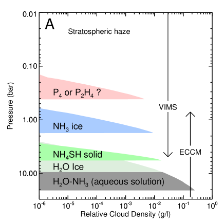
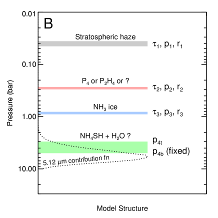
Figure 1.— A: Equilibrium cloud condensation model (ECCM) of the composition and vertical distribution of clouds on Saturn for P $>$ 500 mbar according to Atreya and Wong (2005). All the ECCM clouds have densities expected to greatly exceed actual cloud amounts. For P $<$ 500 mb, a cloud layer of unknown composition (possibly P₄ or P₂H₄) has been inferred from radiation transfer modeling (see text). The density profile of that cloud is chosen for illustrative purposes. According to Sromovsky et al. (2013, 2018) this layer does not display any 3-$\mu$m absorption features and thus cannot be composed entirely of some combination of the materials expected at higher pressures. The downward arrow indicates the pressure depth to which VIMS observations might be sensitive to cloud composition. B: Our model structure containing four sheet clouds corresponding to the expected compositional layers shown in A. Further details are provided in Section 3.4. Also shown is the clear-atmosphere scaled contribution function for emission at 5.12 $\mu$m from Sromovsky et al. (2016).

Evidence of Saturn’s underlying NH₃ ice cloud (its strong 3-$\mu$m absorption signature) has only been evident under unusual circumstances. It has been seen in association with lightning storms, including the Great Storm of 2010-2011 (Sromovsky et al. 2013) near 35^∘N planetocentric latitude, and in much smaller storms located near 36^∘S in the Storm Alley region (Baines et al. 2009). In the Great Storm, strong convection apparently brought NH₃ ice particles to the visible cloud tops. As illustrated in Fig. 2, compared to background clouds, the bright convective cloud at the head of the Great Storm is much darker at 3 $\mu$m than it is at shorter and longer wavelengths. Just where the cloud is brightest at continuum wavelengths, it is also the darkest at 3 $\mu$m. A similar, though less dramatic signature is seen in the bright storm clouds in Storm Alley, also illustrated in Fig. 2. This is consistent with ammonia ice reaching into but not fully penetrating the upper cloud (Sromovsky et al. 2018). In both of these examples, the existence of strong convection was confirmed by the observation of associated lightning. Because no lightning has ever been detected in Saturn’s polar regions, indicating a lack of strong convection, it was surprising to see 3-$\mu$m absorption features in discrete clouds within the eye of the north polar vortex (Baines et al. 2018), as well as in the south polar region that is the subject of this paper. A hint of what might be responsible is the Pérez-Hoyos et al. (2005) finding of a dramatically lower optical depth of the upper tropospheric cloud in the south polar region.

Here we describe quantitative radiative transfer models of both bright and background cloud features. We use their spectral signatures to constrain both composition and vertical structure. We use the difference between observed spectra and spectra computed from aerosol models as constraints on those models. The discussion is organized as follows. We first describe our data selection approach. We then describe the Visual and Infrared Mapping Spectrometer (VIMS) and the observations that we use to gain new insights into the nature of these cloud features. That is followed by descriptions of our approach to radiation transfer modeling, our parameterization of aerosol and gas profiles, and our approach to fitting the observations. Next, we describe the results of fitting background clouds, bright clouds, and dark features. Finally we discuss the implications of these results and summarize our conclusions.

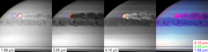
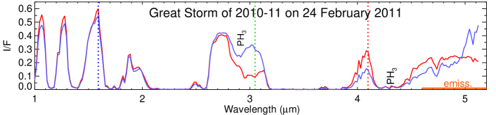
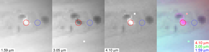
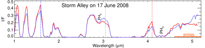
Figure 2.— VIMS observations of the Great Storm (top) and Storm Alley (bottom) illustrate rarely seen spectral signatures of ammonia ice. Blue and red circles identify background and storm clouds respectively. Corresponding spectra are plotted using the same color assignments. The color composite images produce a distinctive magenta color for features with the NH₃ absorption signatures, which include brighter continuum peaks between 1 and 1.6 $\mu$m and at 4.1 $\mu$m, combined with absorption by NH₃ ice near 3 $\mu$m.

2. South polar observations

2.1. Data selection

We selected VIMS observations to take advantage of the near-IR methane bands that can be used to constrain vertical aerosol structures, aerosol composition, and the abundance of arsine and vertical profile for phosphine. Although VIMS also provides visible spectral observations, we decided not to include these in the analysis because they have significant stray light and striping artifacts as well as imaging pointing offsets that create difficulties in analysis of discrete features. The particular VIMS data set we selected provided an optimal compromise between spatial resolution and viewing geometry. The VIMS observations also were made when valuable ISS imaging was available to help understand the latitudinal variations at an even higher spatial resolution than available from VIMS. This is also during the period when ISS imaging was revealing putative eyewalls and cloud shadows, which we hoped to investigate for the first time with quantitative radiation transfer modeling. There are additional observations near this time that provide similar advantages, and could be productively analyzed.

2.2. VIMS instrument characteristics and data reduction

As described by Brown et al. (2004), the VIMS instrument combines two mapping spectrometers, one covering the 0.35-1.0 $\mu$m spectral range, and the second covering an overlapping near-IR range of 0.85-5.12 $\mu$m. The near-IR spectrometer use 256 contiguous channels sampling the spectrum at intervals of approximately 0.016 $\mu$m. The instantaneous field of view of each pixel pair as combined in the observations we used covers 0.5 $\times$ 0.5 milliradians, and a typical frame has dimensions of 64 pixels by 64 pixels. The responsivity of the VIMS near-IR detector array is significantly reduced at joints between order sorting filters, which occur at wavelengths of 1.64 $\mu$m, 2.98 $\mu$m, and 3.85 $\mu$m (Miller et al. 1996; Brown et al. 2004), causing potential calibration uncertainties. We avoided comparisons between models and observations at the most strongly affected regions near 1.64 $\mu$m and 3.85 $\mu$m, but found that the effects of the 2.98-$\mu$m joint were not a significant issue.

The VIMS data sets were reduced using the USGS ISIS3 (Anderson et al. 2004) vimscal program, which was derived from the software provided by the VIMS team (and is available on PDS archive volumes). The radiometric calibration utilized the RC17 calibration (Clark et al. 2012), and conversion to I/F (reflectivity relative to Lambertian reflector normally illuminated) used the solar spectrum packaged with the ISIS3 and PDS-supplied software, which is based on the Drummond and Thekaekara (1973) solar spectrum. The spectra were converted to the more recent RC19 calibration following Sromovsky et al. (2018). Navigation of VIMS cubes (computation of planet coordinates and illumination parameters for each pixel of a VIMS cube) utilized kernels supplied by JPL NAIF system and SPICELIB software (Acton 1996).

Our detailed analysis is based primarily on selected VIMS near-IR observations obtained at 19:35 UT and 20:05 UT on 11 October 2006, which are described more completely in Table 1, along with corresponding observing conditions. For the chosen 2006 observations, a typical solar zenith angle is 75.5^∘ with a typical observer zenith angle of 57^∘. These observations include measurements of reflected sunlight as well as thermal emission, which we found to provide the best combination of constraints on upper and lower cloud parameters and on NH₃ and phosphine (PH₃). Table 1 also includes information about VIMS observations displayed in Fig. 2.

Table 1Observing conditions for VIMS IR data cubes and ISS images used to constrain cloud structure models.

		UT Date	Start	Pixel	Phase	Figure
Observation ID1	Cube Version	YYYY-MM-DD	Time	size	angle	Ref.
030SA_FEATRACK005	V1539288419_1	2006-10-11	19:35:01.6	145 km	37.2∘	5, 16
030SA_FEATRACK005	V1539290255_1	2006-10-11	20:05:37.6	142 km	33.7∘	4
072SA_DYNMOVIE	V1592396725_1	2008-06-17	11:47:35.1	403 km	24.9∘	2
145SA_WIND5HR001	V1677201862_3	2011-02-24	00:36:35.5	883 km	52.0∘	2
ISS image ID	ISS Filter
W1539293298	MT3 (890 nm)	2006-10-11	20:56:08	33.6 km	27.3∘	18
W1539293315	CB2 (752 nm)	2006-10-11	20:56:37	16.8 km	27.3∘	3, 18
W1539293355	MT2 (728 nm)	2006-10-11	20:57:14	16.8 km	27.3∘	18

¹The full observation ID has a leading VIMS_ and suffix _PRIME for rows 3 and 4.

2.3. ISS instrument characteristics and data reduction

We also made use of 2006 observations by the Cassini Imaging Science Subsystem (ISS). The ISS (Porco et al. 2004) has a narrow angle camera (NAC) with a field of view 0.35^∘ across, and a the wide angle camera (WAC) with a FOV of 3.5^∘, both using 1024-pixel square CCD arrays with pixel scales of 1.24 and 12.4 arcseconds/pixel respectively (in the unbinned imaging mode). For our analysis we used WAC images (identified in Table 1), as no relevant NAC images were available. The image files were retrieved from the NASA Planetary Data System’s Imaging Node and processed with the USGS ISIS 3 cisscal application, which is derived from the IDL cisscal application developed by the Cassini Imaging Central Laboratory for Operations (CICLOPS). This cisscal application produces images in I/F units (where a Lambertian reflector, illuminated and viewed normally at the same distance from sun as the target, has an I/F of 1). Ephemeris and pointing data allowing transformations between image and planet coordinates are disseminated by NASA’s Navigation and Ancillary Information Facility (Acton 1996).

2.4. Cassini observations of south polar clouds in 2006

The morphology of Saturn’s south polar region in October of 2006 is illustrated in Fig. 3, where a mosaic of VIMS observations at 2.8 $\mu$m (panel A) is compared with an ISS image taken with a 752-nm filter (panel B). The region from 89^∘S to the pole is quite dark in the VIMS image and bounded by a cloud band edge labeled as the “inner eyewall” in the ISS image. Also note the apparent shadow seen below the top edge of the inner eyewall and the second shadow seen extending from a similar feature labeled as the “outer eyewall”. These features were first analyzed by Dyudina et al. (2008) who inferred, from the shadow geometry, cloud height differences of 40$\pm$20 km at the outer boundary and 70$\pm$30 km for the inner boundary. They also inferred that the top cloud layer extended up into the stratosphere because of boundaries seen in MT-2 and MT-3 methane band images. A possible interpretation of these measurements in the form of a complete cloud profile is shown in Fig. 3C. If the innermost region of the eye, out to about 89^∘, is assumed to be roughly at the level of ammonia condensation, suggesting that the overlying aerosols are either absent or of very low optical depth, then a second cloud top, which would produce the inner shadow, would be expected near the 200 mbar level, which would likely be of the same unknown composition as the ubiquitous upper tropospheric layer commonly found in this region. A second step, up to about 70 mbar, might be at the level of the stratospheric haze.

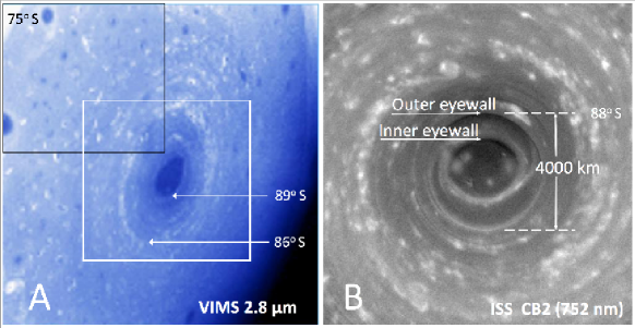
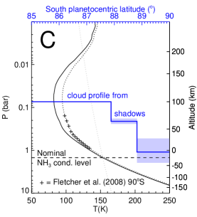
Figure 3.— Views of Saturn’s south polar region on 11 October 2006. The VIMS image at 2.8 $\mu$m (A) is a 7-image mosaic from Baines et al. (2008). The black and white squares indicate the approximate coverage of individual data cubes used in our analysis. The Cassini ISS image (B) is a polar projection of an image taken at 20:56:37.0 UT (following the VIMS observations by about 45 minutes) using a CB2 (752 nm) filter. Its identification number is W1539293315. The very dark region centered in the south pole in the VIMS image corresponds to the region inside what is indicated as the inner “eyewall” in the ISS image (B). Note the apparent shadows at both the inner and outer “eyewall” boundaries in the ISS image (sunlight is incident from the top). The vertical cloud profile (C) is a possible interpretation of cloud heights inferred from the shadows lengths measured by Dyudina et al. (2009). The temperature profile shown as a solid curve is from Lindal et al. (1985) compressed to account for higher gravity at polar latitudes. The dotted curve is the same profile with temperatures scaled to match the 90^∘S profile of Fletcher et al. (2008)

The bright cloud feature just outside the outer wall and intersected by the left end of the dashed line is the same feature seen above the darkest region in the VIMS image. This is in a region of intermediate darkness extending from 89^∘S to 86^∘S. Further from the pole is a somewhat brighter region containing many even brighter small discrete features in both images and a smaller number of small dark features, which are only seen clearly in the VIMS image. There is another step change in cloud properties near 75^∘S (barely visible in the upper left corner of the left panel in Fig. 3), where cloud reflectivity increases, indicating a likely increase in optical depth at that point.

Spectral images and spectra from just outside the inner eye to about 75^∘S are shown in Fig. 4. Many small bright and dark features are seen at pseudo continuum wavelengths of 1.59 $\mu$m and 4.1 $\mu$m, while at 3.05 $\mu$m these bright features appear dark, a familiar characteristic of ammonia clouds seen in the major storm clouds on Saturn (as in Fig. 2). Spectra from a bright feature (3) and from a nearby background region (4) are shown in the bottom panel of the figure, using red and blue colors respectively. Note that the bright feature is only slightly darker than surrounding clouds at 3.05 $\mu$m, but is 20% to 100% brighter at the pseudo continuum wavelengths. This suggests that the underlying ammonia cloud is near its maximum reflectivity for even an infinite optical depth, and that the cloud layer overlying the ammonia layer is sufficiently transparent to see some of the effects of ammonia absorption even in the background region. Also note that the background cloud in this region is very transparent to thermal emission in the 4.6 – 5.1 $\mu$m region, while the bright cloud feature has enough long wavelength absorption to block most of that emission.

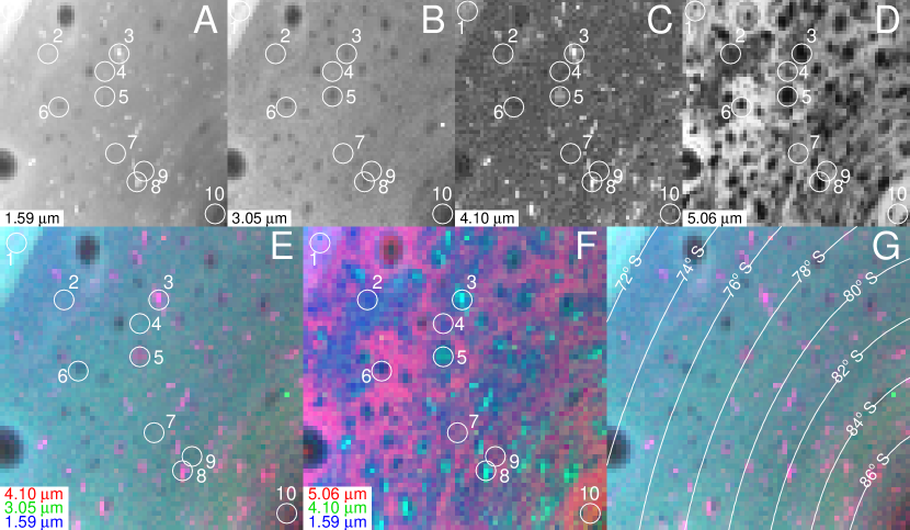
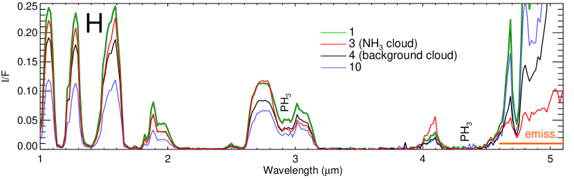
Figure 4.— These 11 October 2006 images from cube V1539290255.1, taken at 20:05 UT (Table 1), cover the region roughly defined by the black square in Fig. 3, using an exposure of 80 ms/pixel, yielding signals well below saturation levels. The top row of panels display image planes at key wavelengths indicated at the lower left of each panel. Panels E (with target circles) and G (with latitude grids) display the same color composite that highlights NH₃ -signature clouds in magenta. Panel F highlights regions of high 5-$\mu$m thermal emission. Panel H plots selected spectra of targets indicated by numbered circles in the image panels. Note that the label “NH₃ cloud” denotes that the cloud feature displays an ammonia spectral signature, not that all the aerosols in the column are made of ammonia.

The color composite image in panels E and G of Fig. 4 displays a characteristic magenta color for the bright features that are dark at 3.05 $\mu$m, which is essentially the same color seen for storm clouds in similar color composites displayed in Fig. 2. All of the small cloud features that are bright at continuum wavelengths in Fig. 4 display a similar color. Note also that some of the dark features are relatively dark at all the key wavelengths (feature 6 for example), which might be a result of a local reduction in optical depth or, less likely, the presence of a broadband absorber. Also note that feature 5, while dark at 3.05 $\mu$m and bright at 4.1 $\mu$m is not brighter than background clouds at 1.59 $\mu$m, which could be a result of larger particles in the ammonia cloud layer that don’t brighten as much at shorter wavelengths. It should be noted that we found no obvious discrete features in any 2-$\mu$m image (not shown), indicating that the bright cloud features do not reach as high as the pressure level to which that wavelength is sensitive (as will be shown later, its two-way optical depth unity level is of the order of 300 mbar).

VIMS images and spectra from the inner eye region out to about 85^∘S are shown in Fig. 5. These images also contain many cloud features (9 and 13 for example) with the spectral signatures of ammonia ice clouds similar to those seen in Fig. 4 and in the storm feature images in Fig. 2. This region has a more organized distribution of ammonia-signature cloud features, with many distributed along a bright ring with an inner edge at about 86^∘S. This ring coincides with a dark ring seen at the thermal emission wavelength of 5.06 $\mu$m (in panel D), which indicates that the total aerosol optical depth above the 4-bar level in this narrow band is quite large. The portion of the eye from about 89^∘S to the pole is relatively dark in reflected sunlight compared to surrounding regions, which is a result of reduced aerosol scattering. This is especially noticeable near 2 $\mu$m (not shown in this figure, but illustrated later in Fig. 16C in Section 5.1), which is a wavelength region sensitive to aerosols in the upper troposphere. On the other hand, the eye is quite bright at thermal emission wavelengths, indicating a reduced level of aerosols at deeper levels. However, the innermost region of the eye is not the brightest region in emission. Somewhat greater emission is seen near 88^∘S, in the region between the inner and outer eye walls (location 8 for example).

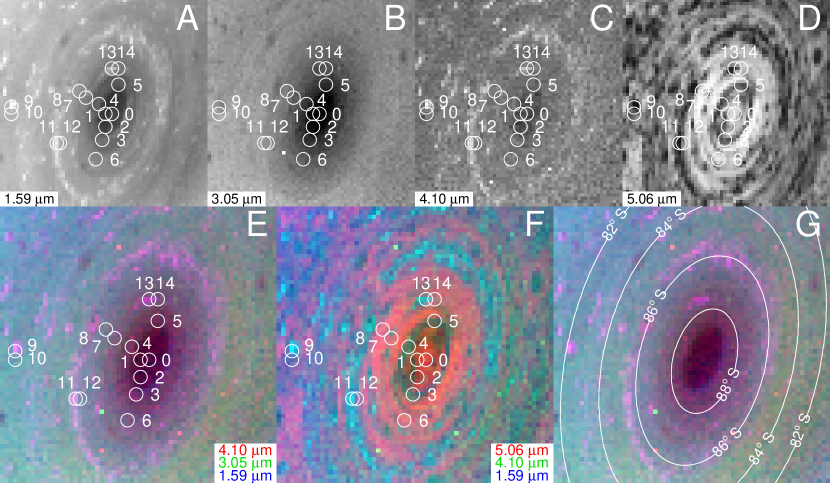
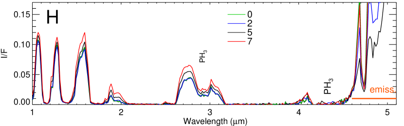
Figure 5.— As in Fig. 4, except that these 11 October 2006 observations are from cube V1539288419 taken at 19:35 UT (Table 1), which covers the inner eye region.

3. Radiative transfer modeling

Before describing the model structure we infer from fitting the observed VIMS spectra we first describe our approach to radiative transfer modeling, i.e. how we parameterized the atmospheric composition, how we model gas absorption and scattering properties of aerosols, and how we handle multiple scattering and thermal emission.

3.1. Atmospheric structure and composition

We generally followed Sromovsky et al. (2013, 2018). We used Lindal et al. (1985) to define the temperature structure between 0.2 mb and 1.3 bars, and approximated the structure at deeper levels using a dry adiabatic extrapolation. The actual temperature structure in the polar region, according to an analysis of Cassini Composite Infrared Spectrometer (CIRS) observations by Fletcher et al. (2008), is somewhat warmer than our assumed profile (as shown in Fig. 3C). At the pole it is warmer by 5–15 K in the 500 – 50 mbar region, but agreement continues to improve with increasing pressures, and much better agreement is obtained a few degrees from from the pole. Although these differences seem large, test calculations for similar differences in the Storm Alley region by Sromovsky et al. (2018) produced spectral differences that were smaller than the uncertainties. We assumed a He/H₂ volume mixing ratio (VMR) of 0.0638 (Lindal et al. 1985). The assumed nominal composition of the atmosphere as a function of pressure is displayed in Fig. 6. For the CH₄ VMR we used the Fletcher et al. (2009b) value (4.7$\pm$0.2)$\times 10^{-3}$, which corresponds to a CH₄/H₂ ratio of 5.3$\times 10^{-3}$. For CH₃D we also used the Fletcher et al. (2009b) VMR value of 3$\times 10^{-7}$. Spectrally, PH₃ is the most important variable gas (significant at 2.8-3.1 $\mu$m and dominant at 4.1-5.1 $\mu$m). Its vertical distribution was adjusted to fit VIMS spectra using a parameterization consisting of an adjustable deep mixing ratio $\alpha_{0}$, a break-point pressure $p_{b}$, and an adjustable scale ratio $f$ of its scale height to the pressure scale height. At pressures less than $p_{b}$, the mixing ratio can be written as

$$\alpha(p)=\alpha_{0}(p/p_{b})^{(1-f)/f}\quad\mathrm{for}\quad p<p_{b}.$$ (1)

Because we found a high correlation between spectral effects of $p_{b}$ and $f$, only two of our three parameters could be well constrained by the VIMS observations. We chose $f$ = 0.1 and fit $p_{b}$ and the deep mixing ratio $\alpha_{0}$.

Arsine (AsH₃) has a noticeable effect on the VIMS spectra near 5 $\mu$m, which is where ammonia gas also plays a relatively minor role. Bézard et al. (1989) derived AsH₃ mixing ratios of 2.4${}^{+1.4}_{-1.2}$ ppb (parts per billion) for the thermal component and 0.39${}^{+0.21}_{-0.13}$ ppb for the reflected solar component. The latter is probably representative of the effective value in the 200 – 400 mbar range where they inferred a haze layer, while the former applies to the deep mixing ratio. Noll et al. (1989) inferred a value of 1.8${}^{+1.8}_{-0.8}$ ppb. Sromovsky et al. (2016) inferred values in the 3.5-7 ppb range for a He/H₂ of 0.064 from spectra in the cleared region following Saturn’s Great Storm of 2010-2011. Fletcher et al. (2011) inferred a value of 2-3 ppb. Our fits in the south polar region ranged from about 1 ppb to 3 ppb.

We initially tried to constrain the NH₃ mixing ratio, but we found that the results were unreliable because of the very low sensitivity of the spectra to the ammonia profile parameters. We eventually decided to fix the ammonia profile, using a deep value of 400 ppm, a pressure break point of 4 bars, at which point we decreased the NH₃ VMR to 3 ppm, finally setting it to the NH₃ saturation mixing ratio for pressures less than the saturation pressure. This profile was loosely guided by the analysis by Briggs and Sackett (1989) of Very Large Array (VLA) radio observations of Saturn, which yielded a deep NH₃ VMR of (4.8 $\pm$1)$\times 10^{-4}$ and some evidence for depletion of NH₃ in the 2-4 bar region, which they interpret as evidence for an NH₄SH cloud and hydrogen sulfide (H₂S) vapor. Our adopted profile was also roughly consistent with the derived base pressure of the cloud layer we assumed to consist of NH₃ ice.

Figure 6.— Volume mixing ratios of spectroscopically important gases in the atmosphere of Saturn. These values were either assumed or derived from fitting the spectrum from the background cloud at location 2. See text for references. The dotted curve traces the saturation vapor pressure profile of NH₃.

3.2. Gas absorption models

We used correlated-k gas absorption models for methane, ammonia, phosphine, arsine, and collision-induced absorption as described by Sromovsky et al. (2018) and references cited therein. For methane we followed Sromovsky et al. (2013) in using correlated-k models based on line-by-line calculations down to 1.268 $\mu$m (Sromovsky et al. 2012), but for shorter wavelengths used correlated-k fits to band models of Karkoschka and Tomasko (2010) (we used P. Irwin’s fits available at http://users.ox.ac.uk/$\sim$atmp0035/ktables/ in files ch4_karkoschka_IR.par.gz and ch4_karkoschka_vis.par.gz). The NH₃ absorption model fits are from Sromovsky and Fry (2010), which are based primarily on band models of Bowles et al. (2008). Absorption models for phosphine (PH₃) and arsine (AsH₃) are the same as described by Sromovsky et al. (2013). Collision-induced absorption (CIA) for H₂ and H₂-He was calculated using programs downloaded from the Atmospheres Node of the Planetary Data System, which are documented by Borysow (1991, 1993) for the H₂-H₂ fundamental band, Zheng and Borysow (1995) for the first H₂-H₂ overtone band, and by Borysow (1992) for H₂-He bands. The vertical penetration depths permitted by these gases individually and in combination are shown in Fig. 7.

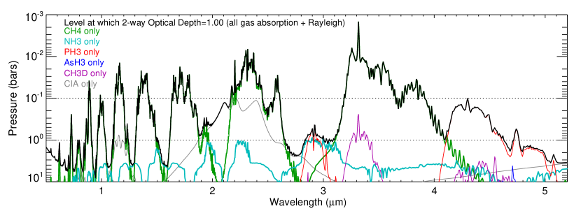
Figure 7.— Penetration depth in a clear atmosphere for various gases singly (colored) and in combination (black), computed for gas mixing ratio profiles are in Fig. 6.

3.3. Cloud composition constraints

3.3.1 Chemical and photochemical constraints

The Equilibrium Cloud Condensation Model (ECCM) provides constraints based on formation theories, chemistry, and thermodynamic properties. An overview of those results was given in Section 1. The main constituents inferred from ECCM are NH₃ ice, NH₄SH, and water ice. However, the vertical distribution suggested by vapor pressure curves can be strongly modified by dynamical considerations, which modify the mixing ratios and condensation levels from those suggested by the simplest interpretation, i.e. that the gases are uniformly mixed up to their condensation levels and above that follow their saturated vapor pressure curves. It is also possible for strong convective events to transport materials upward and produce clouds of mixed composition, with composite particles with a core of one condensate, such as water ice, coated by other condensates such as NH₄SH and NH₃. The Great Storm of 2010-2011 provided one dramatic example of mixed composition being revealed by spectral absorption signatures (Sromovsky et al. 2013). Besides ECCM materials, there are also candidate compounds produced photochemically, the potentially most significant of which are phosphorus (P₄ from photolysis of PH₃), hydrazine (N₂H₄), and diphosphine (P₂H₄).

3.3.2 Spectral constraints

Spectral signatures provide a second important constraint. Refractive index plots for all of the previously discussed materials (except diphosphine and phosphorus, which have not been adequately characterized) are shown in Fig. 8. Among the more plausible compounds, NH₃ has the strongest and sharpest absorption at 2 $\mu$m (the 2.25 $\mu$m absorption feature would not be visible due to overlying gas absorption). NH₄SH has an absorption that is roughly comparable to that of NH₃ at 3 $\mu$m, but lacks a sharp spectral feature and continues to increase beyond 3.1 $\mu$m while NH₃ absorption drops significantly. Hydrazine, which is not expected to be very abundant on Saturn, has a pair of strong absorption peaks between 3 and 3.2 $\mu$m, which would be very apparent unless cloud particles were very large. P₂H₄ appears to have only very weak absorption in this region (Frankiss 1968).

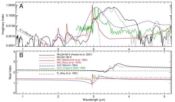
Figure 8.— Imaginary (A) and real (B) components of the refractive index vs. wavelength for candidate 3-$\mu$m absorbers, including H₂O results of Warren (1984), NH₃ results of Roux et al. (1979) and Martonchik et al. (1984), NH₄SH results of Howett et al. (2007), and N₂H₄ results of Clapp and Miller (1996).

3.4. Parameterization of the vertical cloud structure

Based on the above considerations, we assumed a stack of four cloud layers that is summarized in Fig. 1B and Table 2. All layers were assumed to scatter like spherical particles, even though they are most likely composed of solid non-spherical particles. This parameterization scheme was a convenient way to incorporate composition-dependent and wavelength-dependent scattering properties, and because it allowed us to fit most spectra quite well, we were not motivated to try more complex particle models or structures with more parameters to be constrained. We also assumed a gamma size distribution with variance 0.05 to smooth out phase function structure for the stratosphere and a variance of 0.1 for the larger particles of the bottom three layers. The top three layers are essentially sheet clouds, which are characterized by a base pressure, particle size, optical depth, and refractive index. All but the refractive index function are adjustable parameters that are fitted by our retrieval code. The pressures at the top of these layers are large fractions of their base pressures, 0.8 for the top layer, and 0.9 for the second and third layers. These fractions are arbitrary and not constrained by observations. Next we describe how we modeled each of the four layers.

3.4.1 Stratospheric haze (layer 1)

For this top model layer we assumed refractive index of 1.4, which is comparable to the polar value of $\sim$1.45 inferred by Pérez-Hoyos et al. (2005), who assumed that the haze extended from 10 mbar to 1 mbar, but were not able to constrain it any further from their observations. In a subsequent paper Pérez-Hoyos et al. (2016) constrained only the integrated haze optical depth above 100 mbar. Attempts to define the vertical boundaries of this haze in Storm Alley latitudes by Sromovsky et al. (2018) yielded large uncertainties. Nor is the vertical distribution of this haze well constrained our by chosen south polar VIMS observations. We found that a wide range of base pressures and scale heights could provide the same fit quality as a compact haze as long as the optical depth and average pressure were the same. Thus we did not try to define its vertical distribution, but instead fit its effective pressure under the assumption that it is a close to a sheet cloud in vertical extent. In fact, there is good evidence that it might play a role in creating shadows, which would require that it be a relatively compact structure instead of a vertically diffuse structure. We show in the following that its effective pressure is very well constrained by VIMS observations, as are its optical depth and particle size.

3.4.2 Upper tropospheric cloud (layer 2)

The composition of this layer is unknown. As previously noted (Sromovsky et al. 2018, 2016, 2013), while absorbing light at short visible wavelengths (Pérez-Hoyos et al. 2005), this layer appears to have no distinctive absorption features at near-IR wavelengths. Possible compositions include some form of phosphorous or diphosphine. According to a review by Fouchet et al. (2009), diphosphine is a leading candidate. Visscher et al. (2009) predicted a much greater abundance of diphosphine than phosphorus. However, there is currently no spectral evidence for or against diphosphine on Saturn (or on Jupiter). Although it has a distinctive double absorption peak near 4.3 $\mu$m and another absorption feature at 6 $\mu$m (Nixon 1956), these are at least partially masked by phosphine gas absorption and ammonia gas absorption respectively, The degree of masking is uncertain because there is no quantitative characterization of the diphosphine absorption strengths. The white phosphorus (P₄) molecule is a symmetric tetrahedron, has no dipole moment, and is thus unlikely to have any significant near-IR absorption features. We decided to characterize the particles in this layer with a real refractive index of 1.82 (the value for white phosphorus), which is also close to the 1.74 value for P₂H₄ at 195 K (Wohlfarth 2008), the other candidate material for this layer. We chose an imaginary index with the spectral shape defined by Noy et al. (1981) but reduced it by a factor of 10 in amplitude to avoid excessive absorption at short wavelengths. This layer cannot be an ammonia condensate because it contains no 3-$\mu$m absorption feature.

3.4.3 Middle tropospheric cloud (layer 3)

This layer we assumed to consist of ammonia ice particles. This is a plausible assumption because the layer appears in a pressure range where NH₃ is likely to condense, and because this layer clearly has an ammonia ice absorption signature. This layer is found near 1 bar, well above the ECCM-suggested 1.7 bars, presumably due to a depletion of NH₃ by formation of an underlying NH₄SH cloud (Briggs and Sackett 1989). Its pressure is very well constrained by the VIMS observations.

3.4.4 Deep tropospheric cloud (layer 4)

Thermal emission in the 4.6-5.2 $\mu$m spectral region originates from the 2-10 bar level, with the contribution function at 5.12 $\mu$m peaking near 6 bars (Fig. 1), which is determined mainly by collision-induced absorption by hydrogen. However, the emission is attenuated, often significantly, by overlying aerosols in the region between 1.7 and 5 bars where it is possible to have solid condensates comprised of NH₄SH or H₂O or both (Atreya and Wong 2005). As these two materials have different spectral signatures (Fig. 8), there is a reasonable prospect of constraining the composition of this cloud from 5-$\mu$m emission spectra. In their analysis of VIMS night-time emission spectra, Barstow et al. (2016) considered a variety of cloud models for the emission-attenuating layer, obtaining their best fits with a non-scattering cloud of NH₄SH particles, although completely gray particles provided only slightly worse fits. They expressed confidence that whatever the bulk composition of the cloud, if NH₃ or NH₄SH are present they must be contaminated with something that darkens the individual particles and makes them more absorbing. For our model, we assumed the bottom layer to be a diffuse distribution extending from the 5-bar level upwards to a fitted top pressure determined by spectral constraints. We also assumed it to have the same scale height as the atmosphere. We initially used the Howett et al. (2007) index for NH₄SH at 160 K. However, preliminary fits showed that we needed more absorption and spectrally flatter properties than provided by pure NH₄SH. We ultimately adopted a refractive index of 2.0 + 0.03$i$ and a radius of 2 $\mu$m. Thus, our current analysis cannot confirm that this layer actually contains a significant component of NH₄SH.

Table 2Cloud and gas model parameters used in spectral calculations.

Parameter (unit)	Description	Value
$p_{1}$ (bar)	stratospheric haze base pressure	adjustable
$r_{1}$ ($\mu$m)	effective radius of stratospheric particles	adjustable
$n_{1}(\lambda)$	refractive index of stratospheric particles	$n_{1}=1.4$
$\tau_{1}$	stratospheric haze optical depth at 2 $\mu$m	adjustable
$p_{1}$ (bar)	base of main visible cloud layer (P4 or P2H4 ?)	adjustable
$r_{2}$ ($\mu$m)	effective radius of main cloud particles	adjustable
$n_{2}(\lambda)$	refractive index of main cloud	$n_{2}=1.82+i\times 0.1n_{iN}$
$\tau_{2}$	optical depth of upper cloud at 2 $\mu$m	adjustable
$p_{3}$ (bar)	base pressure of putative NH3 cloud	adjustable
$r_{3}$ ($\mu$m)	effective radius of NH3 cloud particles	adjustable
$n_{3}(\lambda)$	refractive index of NH3 cloud particles	same as NH3
$\tau_{3}$	optical depth of NH3 cloud at 2 $\mu$m	adjustable
$p_{4t}$ (bar)	pressure at top of deep cloud (NH4SH + H2O ?)	adjustable
$p_{4b}$ (bar)	bottom of deep cloud	fixed at 5 bars
$r_{4}$ ($\mu$m)	effective radius of deep cloud particles	fixed at 2 $\mu$mor adjusted
$n_{4}(\lambda)$	refractive index of deep cloud particles	2 +$i\times$0.03
$d\tau_{4}/dp$ (bar-1)	optical density of deep cloud at 2 $\mu$m	fixed at 20/bar
$p_{b}$ (bar)	PH3 break-point pressure	adjustable
$\alpha_{0}$	PH3 VMR for $p>p_{b}$	adjustable
$f$	PH3 to H2 scale height ratio for $p<p_{b}$	fixed at 0.1
$AsH_{3}v$	arsine volume mixing ratio	adjustable

NOTE: Sheet clouds are assumed to have a top pressure that is 0.8 (stratosphere) or 0.9 times the bottom pressure and a particle to gas scale height ratio of 1.0; aerosol particles are assumed scatter like spheres with a gamma size distribution with variance parameter $b=0.1$, with distribution function $n(r)=\mbox{constant}\times r^{(1-3b)/b}e^{-r/ab}$, where with $a=r_{\mathrm{i}}$, for $i=0-3$, and $b=$ dimensionless variance, following Hansen and Travis (1974). Optical depths are given for a wavelength of 2 $\mu$m. $n_{iN}$ is the imaginary index determined by Noy et al. (1981).

3.5. Multiple scattering methods

We used the same modified doubling and adding code with thermal source capability that is described by Sromovsky et al. (2013). We used a grid of 56 pressure levels from 0.5 mbar to 40 bars, distributed roughly in equal log increments, except that additional layers are introduced where cloud boundaries are inserted. To model the medium phase angle VIMS observations we used 12 quadrature points per hemisphere in zenith angle and 12 in azimuth. We approximated the line-spread function of the VIMS instrument as a Gaussian with a wavelength-dependent full width at half maximum (FWHM), then collected all the opacity values within $\pm$FWHM of the sample wavelength, weighted those according to the relative amplitude of the line-spread function, then sorted and refit to ten terms again. (The near-IR FWHM values range from 0.0125 $\mu$m to 0.0226 $\mu$m and are available from the Planetary Data System (PDS) at http://atmos.nmsu.edu/data_and_services/atmospheres_data/ cassini/vims.html). A special treatment is required in the 2.95-3.0 $\mu$m region where NH₃ cloud particles have very sharp absorption features. In this region model calculations were made at 5-cm^-1 intervals (the maximum sampling frequency of our correlated-k models) and subsequently smoothed to VIMS resolution.

3.6. Estimation of uncertainties

We used a simplified model of uncertainties in measurement, calibration, and gas absorption modeling, following that suggested by Sromovsky et al. (2016) after comparisons with more complex models. The simplified model expresses the I/F uncertainty as the square root of the sum of two squared quantities. The first is an I/F uncertainty of 0.003 and the second is 10% of the I/F signal. These estimates are meant to capture combined effects of both instrumental and modeling uncertainties, and allow us to fit most observations with $\chi^{2}$ values close to the expected value, which is the number of degrees of freedom N_F, so that $\chi^{2}$/N_F $\approx$ 1, where N_F = number of comparison points (usually 177) less the number of adjusted parameters (13).

Our 1-$\sigma$ uncertainty range for each parameter individually is based on the $\Delta\chi^{2}$ = 1 confidence interval for the $\chi^{2}$ distribution obtained by adjusting all other parameters to minimize $\chi^{2}$ for each value of the chosen parameter (Press et al. 1992). This is estimated by our Levenberg-Marquardt algorithm under the assumption of normally distributed errors, which is not entirely valid. Further, parameter uncertainties we estimate in this fashion are at best only locally valid, and do not guarantee that there is not some other distant solution within this 13-dimensional parameter volume that provides a comparable or better fit. In fact, we did find two distant solutions for the NH₃-signature cloud features, which will be described in Section 4.2. To fully explore this space to find the absolute minimum in $\chi^{2}$ would take an impractically large time because of the complex calculations that are involved and the high dimensionality of the parameter space.

4. Fit Results

We fit observations by first selecting, with guidance from parameter sensitivity calculations described in Sec. 4.5, an a priori model that provides usually only a very rough fit to the observations, and then adjust parameters to minimize $\chi^{2}$ using a form of the Levenberg-Marquardt algorithm as described by Press et al. (1992). A typical fit takes about 2 hours of computation time and usually converges to within 0.2 of the $\chi^{2}$ minimum in 6-15 iterations. In the following, we first consider models of background clouds, then proceed to models of discrete features, and follow that with illustrations of how the model parameters affect the model spectra and how initial values (first guesses) affect final solutions.

4.1. Background cloud models

We fit models to background clouds at locations identified in Figs. 4 and 5. These were segregated into two latitude regions for tabulation. Results for the outer region (from 71.1^∘S to 86.7^∘S) are given in Table 3, and for the inner region (from 87.3^∘S to 89.9^∘S) in Table 4. The cloud structure results for both regions are plotted in Fig. 9, with the black symbols and lines referring to the background cloud structures. These structures do not show very much variation with latitude over most of the outer region, especially within the 73^∘S to 86^∘S latitude band, for which averages and standard deviations are given in Table 5. In most cases the standard deviations are smaller than the estimated uncertainties, indicating that our retrieval error models were somewhat pessimistic. Both layers 1 and 2 show an increased optical depth furthest from the pole, accounting for the higher continuum I/F values seen in the upper left corner of continuum images in Fig. 4. Below we summarize fit results for each aerosol layer. The gas mixing ratio fits will be discussed in Section 4.4.

4.1.1 Stratospheric haze fit results

Over the entire outer region, stratospheric base pressure ranged from 49$\pm$10 mbar to 70$\pm$10 mbar, optical depths ranged from about 0.027$\pm$0.002 to 0.019$\pm$0.005, and the particle radii ranged from 0.18$\pm$0.01 $\mu$m to 0.20$\pm$0.01 $\mu$m, a remarkably small range. Within the restricted outer region (73^∘S to 86^∘S), the average stratospheric optical depth is 0.023 with a standard deviation of only 0.002. The variation is much greater in the inner region, due to the sharp decline in optical depth to 0.0010 as the pole is approached. The transition begins around 86.5^∘S and is complete by 88.5^∘S. There is also a bump in the stratospheric haze altitude centered around 88^∘S, where there is a local pressure minimum near 33-40 mbar.

Table 3Fits to background cloud spectra from 71.1^∘S to 86.7^∘S

Locations:	4-1	4-2	4-4	4-7	5-10	4-9	5-12	5-8
PC Lat.:	-71.1∘	-73.9∘	-77.2∘	-80.1∘	-82.1∘	-82.2∘	-85.8∘	-86.7∘
$p_{1}$, bar	0.050${}^{+0.01}_{-0.01}$	0.049${}^{+0.01}_{-0.01}$	0.055${}^{+0.01}_{-0.01}$	0.056${}^{+0.01}_{-0.01}$	0.061${}^{+0.01}_{-0.01}$	0.059${}^{+0.01}_{-0.01}$	0.070${}^{+0.01}_{-0.01}$	0.055${}^{+0.01}_{-0.01}$
$p_{2}$, bar	0.35${}^{+0.02}_{-0.02}$	0.35${}^{+0.02}_{-0.02}$	0.36${}^{+0.02}_{-0.02}$	0.34${}^{+0.02}_{-0.02}$	0.32${}^{+0.02}_{-0.02}$	0.32${}^{+0.02}_{-0.02}$	0.29${}^{+0.02}_{-0.02}$	0.28${}^{+0.02}_{-0.02}$
$p_{3}$, bar	0.96${}^{+0.16}_{-0.15}$	0.96${}^{+0.17}_{-0.15}$	0.96${}^{+0.25}_{-0.22}$	1.00${}^{+0.27}_{-0.24}$	1.07${}^{+0.34}_{-0.30}$	0.93${}^{+0.23}_{-0.20}$	1.00${}^{+0.23}_{-0.21}$	0.93${}^{+0.18}_{-0.16}$
$p_{4t}$, bar	3.88${}^{+0.07}_{-0.07}$	2.65${}^{+0.04}_{-0.04}$	2.98${}^{+0.04}_{-0.04}$	3.63${}^{+0.06}_{-0.06}$	3.10${}^{+0.05}_{-0.05}$	3.54${}^{+0.05}_{-0.05}$	3.45${}^{+0.05}_{-0.06}$	4.15${}^{+0.08}_{-0.08}$
$\tau_{1}$$\times 10^{2}$	2.65${}^{+0.59}_{-0.49}$	2.46${}^{+0.56}_{-0.46}$	2.53${}^{+0.58}_{-0.47}$	2.34${}^{+0.53}_{-0.44}$	2.19${}^{+0.56}_{-0.45}$	2.17${}^{+0.51}_{-0.42}$	2.31${}^{+0.61}_{-0.48}$	1.85${}^{+0.50}_{-0.39}$
$\tau_{2}$	1.13${}^{+0.09}_{-0.10}$	0.86${}^{+0.10}_{-0.10}$	0.87${}^{+0.11}_{-0.11}$	0.83${}^{+0.09}_{-0.09}$	0.75${}^{+0.08}_{-0.08}$	0.71${}^{+0.10}_{-0.09}$	0.59${}^{+0.10}_{-0.09}$	0.57${}^{+0.08}_{-0.08}$
$\tau_{3}$	1.13${}^{+0.35}_{-0.27}$	0.92${}^{+0.21}_{-0.17}$	0.56${}^{+0.65}_{-0.31}$	0.76${}^{+0.30}_{-0.22}$	0.78${}^{+0.32}_{-0.23}$	0.68${}^{+0.20}_{-0.16}$	0.94${}^{+0.32}_{-0.24}$	0.77${}^{+0.28}_{-0.21}$
$r_{1}$, $\mu$m	0.189${}^{+0.01}_{-0.01}$	0.194${}^{+0.01}_{-0.01}$	0.197${}^{+0.01}_{-0.01}$	0.191${}^{+0.01}_{-0.01}$	0.182${}^{+0.01}_{-0.01}$	0.183${}^{+0.01}_{-0.01}$	0.181${}^{+0.01}_{-0.01}$	0.186${}^{+0.01}_{-0.01}$
$r_{2}$, $\mu$m	0.50${}^{+0.04}_{-0.04}$	0.48${}^{+0.04}_{-0.04}$	0.47${}^{+0.04}_{-0.04}$	0.54${}^{+0.06}_{-0.06}$	0.60${}^{+0.08}_{-0.07}$	0.63${}^{+0.08}_{-0.07}$	0.71${}^{+0.08}_{-0.08}$	0.65${}^{+0.08}_{-0.07}$
$r_{3}$, $\mu$m	1.47${}^{+0.92}_{-0.55}$	1.10${}^{+0.59}_{-0.36}$	1.92${}^{+1.78}_{-0.91}$	1.51${}^{+1.03}_{-0.59}$	1.60${}^{+1.20}_{-0.66}$	1.32${}^{+0.93}_{-0.52}$	1.74${}^{+0.87}_{-0.57}$	1.75${}^{+0.80}_{-0.54}$
$p_{b}$, bar	0.22${}^{+0.05}_{-0.04}$	0.18${}^{+0.07}_{-0.05}$	0.15${}^{+0.07}_{-0.05}$	0.18${}^{+0.05}_{-0.04}$	0.15${}^{+0.06}_{-0.04}$	0.17${}^{+0.05}_{-0.04}$	0.18${}^{+0.04}_{-0.03}$	0.21${}^{+0.03}_{-0.03}$
$\alpha_{0}$, ppm	4.7${}^{+0.2}_{-0.2}$	4.1${}^{+0.4}_{-0.4}$	4.4${}^{+0.3}_{-0.3}$	4.4${}^{+0.2}_{-0.2}$	4.6${}^{+0.3}_{-0.3}$	4.5${}^{+0.2}_{-0.2}$	4.3${}^{+0.3}_{-0.2}$	4.2${}^{+0.2}_{-0.2}$
$AsH_{3}v$, ppb	1.54${}^{+0.33}_{-0.27}$	1.98${}^{+0.56}_{-0.45}$	1.77${}^{+0.45}_{-0.38}$	1.65${}^{+0.30}_{-0.25}$	1.92${}^{+0.42}_{-0.36}$	1.20${}^{+0.31}_{-0.26}$	1.99${}^{+0.39}_{-0.33}$	1.65${}^{+0.33}_{-0.28}$
$\chi^{2}$	204.18	174.85	179.99	184.53	138.96	170.10	148.85	146.10
$\chi^{2}/N_{F}$	1.25	1.07	1.10	1.13	0.85	1.04	0.91	0.89

NOTE: These fits cover the spectral range from 0.88 $\mu$m to 5.12 $\mu$m, with exclusions for order sorting filter joints and regions with very low S/N ratios. These fits assumed fixed values of $p_{4}$ = 5 bars, $r_{4}$ = 2 $\mu$m, and $f$ = 0.1.

4.1.2 Layer-2 (P₄ or P₂H₄?) fit results

The putative diphosphine layer has even less variability than the stratospheric haze. Its base pressure smoothly decreases from about 350 mbar at 71^∘S to 290 mbar near 87.5^∘S, then increases to 400 mbar as the pole is approached. Its optical depth declines towards the pole, from near unity at 71^∘S, then slowly with latitude until about 86^∘S, then more rapidly until it reaches a low of 0.31$\pm$0.1 near the pole. Both vertical descent and decreasing optical depth are consistent with downwelling motion as the pole is approached. The optical depth transition for this layer is close to the edge of a sharp brightness decrease seen in ISS and VIMS images that can sense scattering at the level of this layer, which is also the boundary associated with shadows seen at continuum wavelengths. A further drop from that point towards the pole seems to be the main cause for the dark polar eye when viewed at solar reflected wavelengths. This decrease in the optical depth of the putative diphosphine layer results in a partial unmasking of the ammonia signature to such a degree that the entire region within 2^∘ of the pole can be considered an ammonia-signature cloud structure. This is also evident from the magenta color it displays in Fig. 5E/G.

4.1.3 Ammonia layer fit results

An even more muted variation is seen for the background NH₃ cloud layer. Its pressure is almost invariant with latitude all the way to the pole, although the uncertainty in our constraints of this parameter results in a higher standard deviation than for the layer 2 pressures. Its pressure averaged 979 mbar ($\sigma$ = 46 mbar) in the restricted outer region (73^∘S to 86^∘S), and declined to 810 mbar close to the pole, rising upward slightly (in altitude) against the trend of the layers above it, which both move downward near the pole. Its optical depth remains relatively close to its restricted outer mean of 1.05 ($\sigma$ = 0.13), but also has a slight decline towards the pole, by about 20%, a much smaller fraction than for other layers. Perhaps this indicates that the downwelling motion stops near the level of the NH₃ cloud. However, there is a decrease in particle radius near the pole where it declines from near 2 $\mu$m near 87^∘S by almost a factor of two near 90^∘S.

4.1.4 Bottom layer fit results

The top pressure of the deep cloud varies as needed to match the rather patchy spatial variation in 5-$\mu$m emissions, varying from 2.7 bars to 4.1 bars, with the inner region containing the larger values. However, variations in this layer do not seem to be correlated with changes in the overlying layers, with the one exception being close to the pole. This is not necessarily a trend, however, because there is quite a lot of spatial structure at thermal emission wavelengths that was not adequately sampled by our small number of selected spectra. For the background cloud structures the upper three layers seem disconnected from the variations that occur in the 2.7-5 bar region. In the following we show that this disconnection is not the case for the ammonia signature features.

Table 4Fits to background cloud spectra at locations from 87.3^∘S to 89.8^∘S.

Locations:	5-7	5-6	5-14	5-5	5-4	5-3	5-2	5-1	5-0
PC Lat.:	-87.3∘	-87.5∘	-87.6∘	-88.4∘	-88.5∘	-88.6∘	-89.2∘	-89.3∘	-89.8∘
$p_{1}$, bar	0.054${}^{+0.01}_{-0.01}$	0.040${}^{+0.01}_{-0.01}$	0.041${}^{+0.01}_{-0.01}$	0.040${}^{+0.02}_{-0.01}$	0.033${}^{+0.02}_{-0.01}$	0.044${}^{+0.02}_{-0.01}$	0.058${}^{+0.02}_{-0.02}$	0.056${}^{+0.02}_{-0.02}$	0.061${}^{+0.02}_{-0.02}$
$p_{2}$, bar	0.30${}^{+0.02}_{-0.02}$	0.29${}^{+0.02}_{-0.02}$	0.27${}^{+0.02}_{-0.02}$	0.32${}^{+0.03}_{-0.03}$	0.30${}^{+0.03}_{-0.02}$	0.33${}^{+0.03}_{-0.03}$	0.41${}^{+0.05}_{-0.05}$	0.41${}^{+0.05}_{-0.04}$	0.43${}^{+0.05}_{-0.04}$
$p_{3}$, bar	0.89${}^{+0.16}_{-0.14}$	0.87${}^{+0.17}_{-0.15}$	0.82${}^{+0.09}_{-0.08}$	0.84${}^{+0.14}_{-0.13}$	0.82${}^{+0.09}_{-0.09}$	0.84${}^{+0.13}_{-0.12}$	0.85${}^{+0.20}_{-0.18}$	0.81${}^{+0.11}_{-0.10}$	0.81${}^{+0.10}_{-0.09}$
$p_{4t}$, bar	3.80${}^{+0.06}_{-0.07}$	4.15${}^{+0.08}_{-0.09}$	3.62${}^{+0.06}_{-0.06}$	2.94${}^{+0.04}_{-0.04}$	2.72${}^{+0.03}_{-0.03}$	3.16${}^{+0.05}_{-0.05}$	3.37${}^{+0.05}_{-0.05}$	3.52${}^{+0.04}_{-0.04}$	3.88${}^{+0.07}_{-0.07}$
$\tau_{1}$$\times 10^{2}$	1.50${}^{+0.43}_{-0.33}$	1.14${}^{+0.32}_{-0.25}$	1.13${}^{+0.35}_{-0.27}$	0.90${}^{+0.30}_{-0.23}$	0.76${}^{+0.27}_{-0.20}$	0.96${}^{+0.31}_{-0.23}$	0.91${}^{+0.29}_{-0.22}$	0.97${}^{+0.31}_{-0.23}$	1.03${}^{+0.30}_{-0.23}$
$\tau_{2}$	0.51${}^{+0.08}_{-0.08}$	0.52${}^{+0.09}_{-0.08}$	0.44${}^{+0.07}_{-0.06}$	0.44${}^{+0.08}_{-0.07}$	0.43${}^{+0.07}_{-0.06}$	0.43${}^{+0.09}_{-0.08}$	0.37${}^{+0.13}_{-0.10}$	0.32${}^{+0.09}_{-0.08}$	0.31${}^{+0.10}_{-0.08}$
$\tau_{3}$	0.73${}^{+0.29}_{-0.21}$	0.81${}^{+0.32}_{-0.23}$	0.93${}^{+0.23}_{-0.19}$	0.70${}^{+0.27}_{-0.20}$	0.86${}^{+0.23}_{-0.18}$	0.99${}^{+0.23}_{-0.19}$	0.64${}^{+0.26}_{-0.18}$	0.70${}^{+0.19}_{-0.15}$	0.79${}^{+0.21}_{-0.17}$
$r_{1}$, $\mu$m	0.182${}^{+0.01}_{-0.01}$	0.181${}^{+0.01}_{-0.01}$	0.181${}^{+0.01}_{-0.01}$	0.179${}^{+0.02}_{-0.01}$	0.170${}^{+0.02}_{-0.02}$	0.178${}^{+0.02}_{-0.01}$	0.173${}^{+0.02}_{-0.02}$	0.180${}^{+0.02}_{-0.01}$	0.183${}^{+0.02}_{-0.01}$
$r_{2}$, $\mu$m	0.65${}^{+0.08}_{-0.07}$	0.65${}^{+0.08}_{-0.07}$	0.62${}^{+0.08}_{-0.07}$	0.59${}^{+0.07}_{-0.07}$	0.62${}^{+0.07}_{-0.06}$	0.58${}^{+0.08}_{-0.07}$	0.61${}^{+0.11}_{-0.09}$	0.62${}^{+0.12}_{-0.10}$	0.60${}^{+0.13}_{-0.11}$
$r_{3}$, $\mu$m	2.00${}^{+0.71}_{-0.52}$	2.04${}^{+0.73}_{-0.54}$	1.70${}^{+0.44}_{-0.35}$	1.75${}^{+0.56}_{-0.42}$	1.78${}^{+0.44}_{-0.35}$	1.34${}^{+0.45}_{-0.33}$	1.24${}^{+0.54}_{-0.36}$	1.28${}^{+0.46}_{-0.33}$	1.05${}^{+0.42}_{-0.29}$
$p_{b}$, bar	0.22${}^{+0.05}_{-0.04}$	0.21${}^{+0.03}_{-0.02}$	0.23${}^{+0.03}_{-0.03}$	0.25${}^{+0.04}_{-0.03}$	0.26${}^{+0.04}_{-0.03}$	0.28${}^{+0.04}_{-0.03}$	0.33${}^{+0.07}_{-0.06}$	0.39${}^{+0.07}_{-0.06}$	0.40${}^{+0.05}_{-0.04}$
$\alpha_{0}$, ppm	4.5${}^{+0.2}_{-0.2}$	4.2${}^{+0.2}_{-0.2}$	4.3${}^{+0.2}_{-0.2}$	4.3${}^{+0.3}_{-0.3}$	4.1${}^{+0.3}_{-0.3}$	4.6${}^{+0.3}_{-0.3}$	4.2${}^{+0.2}_{-0.2}$	4.3${}^{+0.2}_{-0.2}$	4.1${}^{+0.2}_{-0.2}$
$AsH_{3}v$, ppb	1.37${}^{+0.30}_{-0.25}$	1.63${}^{+0.30}_{-0.25}$	1.32${}^{+0.28}_{-0.23}$	1.24${}^{+0.36}_{-0.29}$	1.15${}^{+0.36}_{-0.28}$	1.10${}^{+0.24}_{-0.19}$	1.08${}^{+0.24}_{-0.20}$	1.24${}^{+0.26}_{-0.21}$	1.14${}^{+0.24}_{-0.20}$
$\chi^{2}$	134.05	150.34	148.52	128.59	125.36	128.33	133.19	153.03	152.91
$\chi^{2}/N_{F}$	0.82	0.92	0.91	0.78	0.76	0.78	0.81	0.93	0.93

NOTE: These fits cover the spectral range from 0.88 $\mu$m to 5.12 $\mu$m, with exclusions for order sorting filter joints and regions with very low S/N ratios. These fits assumed fixed values of $p_{4}$ = 5 bars, $r_{4}$ = 2 $\mu$m, $f$ = 0.1, and $d\tau_{4}/dp$ = 20/bar.

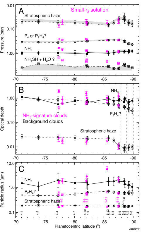
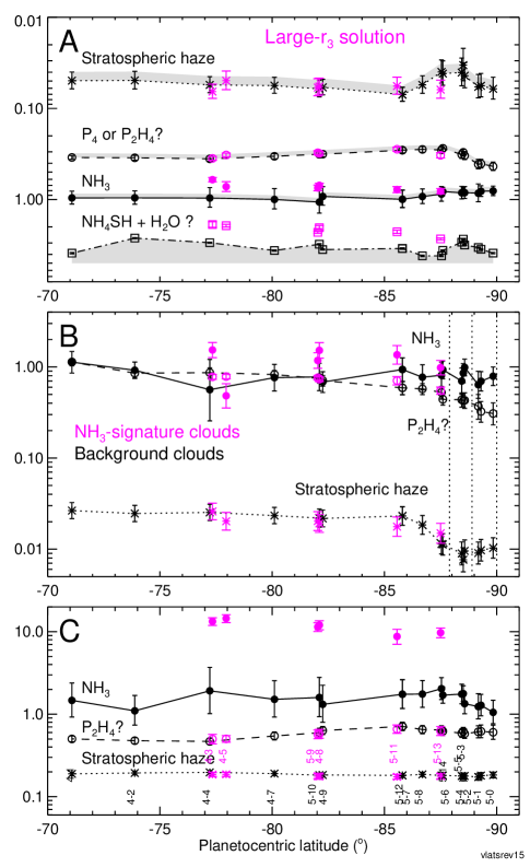
Figure 9.— Best-fit model parameters for background clouds (black) and NH₃-signature clouds (magenta). The left column displays the small-$r_{3}$ solutions for the NH₃-signature clouds, and the right column the large-$r_{3}$ solutions. In each column, panel A displays pressures versus latitude for the putative diphosphine layer (open circles), the NH₃ layer (filled circles), and the top of the bottom layer (squares). Optical depths (B) and particle radii (C) are plotted for the top three layers. The location numbers referred to in Figs. 4 and 5 are noted above the x-axis in panel C. The ammonia-signature clouds have larger particles and larger optical depths than the background clouds, and deep cloud tops that extend to higher altitudes. Dotted vertical lines at 87.9^∘S and 88.9^∘S mark locations of brightness step changes in ISS 752-nm images (discussed in Sec. 5.1.)

Table 5Mean, standard deviation of fitted values about their mean, and uncertainty of the mean, for fits to background and large-$r_{3}$ and small-$r_{3}$ fits to ammonia-signature clouds within the latitude band from 73^∘S to 86^∘S, where other parameters are relatively independent of latitude.

	Background (N=6)			NH3-sig., large $r_{3}$ (N=4)			NH3-sig., small $r_{3}$ (N=4)
Par., unit	mean	$\sigma$	$\sigma/\sqrt{N-1}$	mean	$\sigma$	$\sigma/\sqrt{N-1}$	mean	$\sigma$	$\sigma/\sqrt{N-1}$
p1, bar	0.060	0.008	0.003	0.058	0.006	0.003	0.058	0.008	0.003
p2, bar	0.317	0.029	0.010	0.315	0.027	0.012	0.272	0.012	0.006
p3, bar	0.979	0.046	0.016	0.710	0.066	0.029	0.733	0.091	0.041
p4t, bar	3.369	0.458	0.162	2.084	0.188	0.084	1.915	0.271	0.121
$\tau_{1}$ x 100	2.270	0.209	0.074	2.068	0.313	0.140	1.834	0.263	0.118
$\tau_{2}$	0.720	0.123	0.044	0.754	0.032	0.014	0.600	0.119	0.053
$\tau_{3}$	0.795	0.134	0.047	1.216	0.435	0.195	1.292	0.452	0.202
r1, $\mu$m	0.187	0.006	0.002	0.180	0.006	0.003	0.172	0.004	0.002
r2, $\mu$m	0.599	0.096	0.034	0.562	0.066	0.029	0.572	0.057	0.025
r3, $\mu$m	1.586	0.269	0.095	12.019	2.175	0.973	2.682	1.565	0.700
pb, bar	0.177	0.019	0.007	0.245	0.045	0.020	0.179	0.035	0.016
$\alpha_{0}$, ppm	4.343	0.181	0.064	9.428	3.186	1.425	5.330	0.841	0.376
$AsH_{3}v$, ppb	1.769	0.272	0.096	2.542	0.554	0.248	1.322	0.325	0.145
$\chi^{2}$/$N_{F}$	0.985	0.108	0.038	1.089	0.111	0.050	1.265	0.304	0.136

NOTE: The averages are unweighted, $\sigma$ is the standard deviation of fits about the mean and $\sigma/\sqrt{N-1}$ is the estimated uncertainty of the mean.

4.2. Models of ammonia-signature clouds

The ammonia signature clouds are taken to be those that appear brighter than background clouds at pseudo-continuum wavelengths of 1.59 $\mu$m and 4.1 $\mu$m, while being darker than or at least no brighter than background clouds at 3.05 $\mu$m, a wavelength at which NH₃ ice absorbs strongly. These are the cloud features that have a magenta color in panels E and G of Figs. 4 and 5. Two different solutions were found for the ammonia-signature features: a solution with a small (1-2 $\mu$m) particle radius in the ammonia layer (layer 3), and a second solution with a much larger (10-13 $\mu$m) particle radius in the ammonia layer, comparable to the 14-$\mu$m ammonia particle radius found by Baines et al. (2018) for a bright feature in the north polar eye. The best-fit model results are plotted in Fig. 9 using a magenta color, with parameter values and uncertainties given in Table 6. Here the left column is for the small-$r_{3}$ solutions and the right column is for the large-$r_{3}$ solutions. The same background structure is plotted in both columns for reference. Average characteristics over the restricted outer region are also given for both solutions in Table 5, along with standard deviations, and uncertainty estimates for the averages. The larger particle solution produces slightly better overall fit qualities and in some cases makes significant improvements in local regions where ammonia spectral signatures are more evident. This is illustrated in Fig. 10, which provides a comparison of measured spectra with corresponding model spectra at background location 4-4 and NH₃ -signature spectra at location 4-3. Here the improvement provided by the large-$r_{3}$ solution is significant and is obvious near 3 $\mu$m and 4.1 $\mu$m. But there are other cases in which the alternate solutions are of comparable quality, which can be seen by comparing $\chi^{2}$ values in Tables 6 and 7. Although there is no fit for which the small-$r_{3}$ solution is better than the large-$r_{3}$ solution, we kept both because in several cases the differences are insignificant, and in all cases the large-$r_{3}$ solutions are accompanied by significantly different gas mixing ratios compared to background fits, while the small-$r_{3}$ solutions are in better agreement with the background model gas parameters (discussed in Sec. 4.4). On the other hand, the large-$r_{3}$ solutions are more consistent with background optical depths and particle sizes for the stratospheric haze, and with particle sizes and pressures for the putative diphosphine layer.

Table 6Fits to NH₃-signature cloud spectra, small $r_{3}$ solution from all regions.

Locations:	4-3	4-5	5-9	4-8	5-11	5-13
PC. Lat.	-77.3∘	-77.9∘	-82.0∘	-82.1∘	-85.6∘	-87.5∘
$p_{1}$, bar	0.071${}^{+0.015}_{-0.014}$	0.051${}^{+0.014}_{-0.012}$	0.053${}^{+0.015}_{-0.013}$	0.058${}^{+0.014}_{-0.012}$	0.056${}^{+0.013}_{-0.012}$	0.044${}^{+0.015}_{-0.012}$
$p_{2}$, bar	0.26${}^{+0.03}_{-0.03}$	0.28${}^{+0.03}_{-0.02}$	0.26${}^{+0.02}_{-0.02}$	0.28${}^{+0.02}_{-0.02}$	0.28${}^{+0.02}_{-0.01}$	0.29${}^{+0.03}_{-0.02}$
$p_{3}$, bar	0.59${}^{+0.03}_{-0.03}$	0.71${}^{+0.08}_{-0.08}$	0.77${}^{+0.06}_{-0.06}$	0.76${}^{+0.06}_{-0.06}$	0.83${}^{+0.07}_{-0.06}$	0.85${}^{+0.08}_{-0.08}$
$p_{4t}$, bar	1.52${}^{+0.16}_{-0.15}$	1.89${}^{+0.06}_{-0.05}$	2.18${}^{+0.04}_{-0.04}$	1.83${}^{+0.06}_{-0.06}$	2.16${}^{+0.06}_{-0.06}$	2.57${}^{+0.04}_{-0.04}$
$\tau_{1}$$\times 10^{2}$	2.29${}^{+0.80}_{-0.60}$	1.80${}^{+0.58}_{-0.44}$	1.62${}^{+0.55}_{-0.41}$	1.75${}^{+0.54}_{-0.41}$	1.71${}^{+0.48}_{-0.37}$	1.06${}^{+0.36}_{-0.27}$
$\tau_{2}$	0.41${}^{+0.06}_{-0.06}$	0.62${}^{+0.08}_{-0.08}$	0.58${}^{+0.07}_{-0.06}$	0.65${}^{+0.08}_{-0.07}$	0.73${}^{+0.07}_{-0.07}$	0.49${}^{+0.07}_{-0.07}$
$\tau_{3}$	1.95${}^{+0.29}_{-0.26}$	0.88${}^{+0.34}_{-0.25}$	1.57${}^{+0.35}_{-0.29}$	1.03${}^{+0.32}_{-0.25}$	1.04${}^{+0.23}_{-0.19}$	1.23${}^{+0.38}_{-0.30}$
$r_{1}$, $\mu$m	0.171${}^{+0.013}_{-0.012}$	0.179${}^{+0.012}_{-0.011}$	0.169${}^{+0.013}_{-0.012}$	0.171${}^{+0.013}_{-0.012}$	0.172${}^{+0.012}_{-0.011}$	0.175${}^{+0.014}_{-0.013}$
$r_{2}$, $\mu$m	0.58${}^{+0.13}_{-0.11}$	0.50${}^{+0.06}_{-0.05}$	0.57${}^{+0.08}_{-0.07}$	0.55${}^{+0.07}_{-0.06}$	0.66${}^{+0.08}_{-0.07}$	0.57${}^{+0.07}_{-0.06}$
$r_{3}$, $\mu$m	1.68${}^{+0.28}_{-0.24}$	1.78${}^{+0.54}_{-0.41}$	1.83${}^{+0.39}_{-0.32}$	2.76${}^{+0.70}_{-0.56}$	5.37${}^{+1.54}_{-1.26}$	2.03${}^{+0.51}_{-0.41}$
$p_{b}$, bar	0.21${}^{+0.04}_{-0.03}$	0.21${}^{+0.03}_{-0.03}$	0.17${}^{+0.06}_{-0.04}$	0.13${}^{+0.07}_{-0.05}$	0.18${}^{+0.04}_{-0.03}$	0.18${}^{+0.05}_{-0.04}$
$\alpha_{0}$, ppm	5.3${}^{+0.7}_{-0.6}$	4.9${}^{+0.7}_{-0.6}$	4.3${}^{+0.6}_{-0.5}$	5.6${}^{+1.1}_{-0.9}$	6.6${}^{+1.2}_{-1.0}$	4.1${}^{+0.4}_{-0.4}$
$AsH_{3}v$, ppb	1.15${}^{+0.46}_{-0.33}$	1.06${}^{+0.44}_{-0.31}$	1.12${}^{+0.42}_{-0.31}$	1.44${}^{+0.55}_{-0.40}$	1.84${}^{+0.62}_{-0.49}$	0.99${}^{+0.37}_{-0.27}$
$\chi^{2}$	282.14	193.41	178.86	229.21	153.61	154.14
$\chi^{2}/N_{F}$	1.72	1.18	1.09	1.40	0.94	0.94

NOTE: These fits cover the spectral range from 0.88 $\mu$m to 5.12 $\mu$m, with exclusions for order sorting filter joints and regions with very low S/N ratios. These fits assumed fixed values of $p_{4}$ = 5 bars, $r_{4}$ = 2 $\mu$m, $f$ = 0.1, and $d\tau_{4}/dp$ = 20/bar.

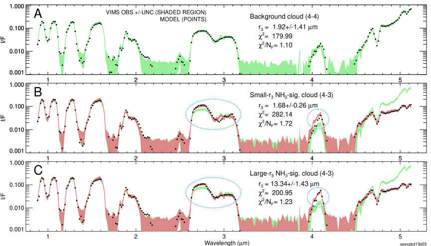
Figure 10.— (A:) Model spectrum (points) compared to observed background spectrum from location 4-4 (light green shaded region, with shading indicating combined uncertainty of measurement and modeling). (B:) As in A except the model is the small-$r_{3}$ fit to the NH₃ signature spectrum from location 4-3, with shading in red, and background spectrum from A shown with green shading. (C:) As in B, except the model spectrum is for the large-$r_{3}$ solution, which provides a significantly better fit in this case, especially in regions within dotted blue ovals.

Table 7Fits to NH₃-signature cloud spectra, large $r_{3}$ solution from all regions.

Locations:	4-3	4-5	5-9	4-8	5-11	5-13
Planetocent. Lat.	-77.3∘	-77.9∘	-82.0∘	-82.1∘	-85.6∘	-87.5∘
$p_{1}$, bar	0.065${}^{+0.012}_{-0.011}$	0.050${}^{+0.013}_{-0.011}$	0.059${}^{+0.013}_{-0.012}$	0.057${}^{+0.012}_{-0.011}$	0.057${}^{+0.013}_{-0.011}$	0.062${}^{+0.015}_{-0.013}$
$p_{2}$, bar	0.35${}^{+0.02}_{-0.02}$	0.32${}^{+0.02}_{-0.02}$	0.31${}^{+0.02}_{-0.02}$	0.31${}^{+0.02}_{-0.02}$	0.28${}^{+0.02}_{-0.01}$	0.33${}^{+0.02}_{-0.02}$
$p_{3}$, bar	0.61${}^{+0.03}_{-0.03}$	0.72${}^{+0.09}_{-0.09}$	0.75${}^{+0.05}_{-0.05}$	0.70${}^{+0.04}_{-0.04}$	0.78${}^{+0.06}_{-0.06}$	0.81${}^{+0.06}_{-0.05}$
$p_{4t}$, bar	1.88${}^{+0.13}_{-0.13}$	1.94${}^{+0.07}_{-0.07}$	2.30${}^{+0.06}_{-0.06}$	2.04${}^{+0.11}_{-0.11}$	2.26${}^{+0.09}_{-0.09}$	2.71${}^{+0.07}_{-0.07}$
$\tau_{1}$$\times 10^{2}$	2.59${}^{+0.60}_{-0.49}$	2.03${}^{+0.50}_{-0.41}$	2.03${}^{+0.55}_{-0.43}$	1.92${}^{+0.49}_{-0.39}$	1.77${}^{+0.49}_{-0.38}$	1.49${}^{+0.43}_{-0.33}$
$\tau_{2}$	0.78${}^{+0.05}_{-0.05}$	0.78${}^{+0.04}_{-0.04}$	0.76${}^{+0.04}_{-0.04}$	0.73${}^{+0.04}_{-0.04}$	0.71${}^{+0.07}_{-0.07}$	0.55${}^{+0.05}_{-0.05}$
$\tau_{3}$	1.54${}^{+0.32}_{-0.27}$	0.48${}^{+0.17}_{-0.13}$	1.18${}^{+0.25}_{-0.21}$	1.52${}^{+0.33}_{-0.28}$	1.36${}^{+0.36}_{-0.29}$	0.98${}^{+0.20}_{-0.17}$
$r_{1}$, $\mu$m	0.185${}^{+0.011}_{-0.010}$	0.187${}^{+0.011}_{-0.011}$	0.177${}^{+0.012}_{-0.011}$	0.176${}^{+0.012}_{-0.011}$	0.174${}^{+0.012}_{-0.011}$	0.177${}^{+0.013}_{-0.012}$
$r_{2}$, $\mu$m	0.50${}^{+0.07}_{-0.06}$	0.50${}^{+0.05}_{-0.04}$	0.57${}^{+0.07}_{-0.07}$	0.58${}^{+0.08}_{-0.07}$	0.66${}^{+0.08}_{-0.07}$	0.63${}^{+0.08}_{-0.07}$
$r_{3}$, $\mu$m	13.34${}^{+1.43}_{-1.43}$	14.52${}^{+1.58}_{-1.61}$	11.44${}^{+1.43}_{-1.38}$	12.03${}^{+1.53}_{-1.49}$	8.76${}^{+1.93}_{-1.73}$	9.74${}^{+1.37}_{-1.29}$
$p_{b}$, bar	0.32${}^{+0.04}_{-0.04}$	0.23${}^{+0.06}_{-0.05}$	0.21${}^{+0.04}_{-0.03}$	0.26${}^{+0.03}_{-0.03}$	0.21${}^{+0.03}_{-0.02}$	0.20${}^{+0.05}_{-0.04}$
$\alpha_{0}$, ppm	12.8${}^{+2.5}_{-2.2}$	6.7${}^{+1.3}_{-1.1}$	6.6${}^{+0.9}_{-0.8}$	12.9${}^{+1.9}_{-1.7}$	8.2${}^{+1.1}_{-1.0}$	5.6${}^{+0.5}_{-0.5}$
$AsH_{3}v$, ppb	3.24${}^{+0.96}_{-0.83}$	2.07${}^{+0.80}_{-0.61}$	2.95${}^{+0.83}_{-0.70}$	2.50${}^{+0.76}_{-0.63}$	1.95${}^{+0.67}_{-0.52}$	1.66${}^{+0.51}_{-0.40}$
$\chi^{2}$	200.95	181.96	174.57	184.57	150.86	154.94
$\chi^{2}/N_{F}$	1.23	1.11	1.06	1.13	0.92	0.94

NOTE: These fits cover the spectral range from 0.88 $\mu$m to 5.12 $\mu$m, with exclusions for order sorting filter joints and regions with very low S/N ratios. These fits assumed fixed values of $p_{4}$ = 5 bars, $r_{4}$ = 2 $\mu$m, $f$ = 0.1, and $d\tau_{4}/dp$ = 20/bar.

The most consistent characteristic of the NH₃-signature cloud structures is that they provide a strong blocking of Saturn’s thermal emission. But in those structures the cloud layer that provides almost all the blocking is the deep cloud, not the ammonia cloud. The deep cloud layer extends upwards to much lower pressures than is typical for the background clouds, averaging 1.9$\pm$0.12 bars compared to the background average of 3.24$\pm$0.16 bars, both in the outer region, where the uncertainties of the unweighted averages are computed as $\sigma$/$\sqrt{(N-1)}$. The effect of these deep clouds is mainly restricted to the thermal emission spectral region, although they do provide a small boost to the continuum spectra at wavelengths less than 1.65 $\mu$m (as evident from derivative spectra shown in Section 4.5). We chose a model in which the base of the deep cloud is fixed at 5 bars and has a fixed optical density, but an adjustable (fitted) cloud top. This choice is consistent with the idea that vertical convection elevates cloud particles to pressures low enough to block thermal emission. It also would have been possible to attenuate thermal emission with a suspended sheet cloud, although that structure is less appealing on dynamical grounds.

For the NH₃-signature structures in the outer restricted region, the elevation of the deep cloud is accompanied by a smaller local elevation of the NH₃ cloud layer, from 979$\pm$16 mbar to 710$\pm$29 mbar or 733$\pm$41 mbar for large and small $r_{3}$ solutions respectively, as well as an increase in its optical depth from 0.80$\pm$0.05 to an average of 1.22$\pm$0.20 or 1.29$\pm$0.20. The NH₃–signature cloud structures have significant variability in the ammonia layer, and very little variability in the putative diphosphine layer. The NH₃ spectral signature for the discrete feature we analyzed closest to the pole (5-13 at 87.5^∘S) is made more obvious by the small 0.49 optical depth of the diphosphine layer.

4.3. Comparison of background and NH₃-signature cloud structures

The most consistent feature of the NH₃-signature clouds, compared to background clouds, is the relatively low top pressure of their deep NH₄SH +H₂O layer, which makes that layer more effective in blocking Saturn’s thermal emission. All the NH₃-signature clouds have this feature. Most of the background clouds have the top of this layer about 1 bar deeper, although there are a few background clouds that have thicker bottom layers. Three examples of NH₃-signature cloud structures in comparison with nearby background cloud structures are shown in Fig. 11. For the left hand pair, from near 77^∘S, the main differences of the NH₃-signature structure from the background structure are (1) all the cloud layers are elevated relative to the background, most dramatically for the top of the deep layer, which moved from 3 bars to 1.5 bars, (2) the optical depth of the ammonia layer is up by more than a factor of two, and (3) the optical depth of the putative diphosphine layer is slightly lower. The elevated top of the deep layer suggests that deep convection is responsible for initiating the other observed effects.

For the NH₃-signature structures, the elevation of the NH₃ layer and its increased opacity is a plausible consequence of the Taylor-Proudman theorem, in which Coriolis forces prevent motion perpendicular to the rotation axis (Pedlosky 1982). Thus a pulse of deep convection can push higher cloud layers upward, without convective penetration of those layers, as if the column above the convective pulse were confined by vertical walls confining the motion of gases within it. The fact that the putative diphosphine layer does not exhibit an optical depth increase, or much elevation for the large-$r_{3}$ solution, seems to contradict this idea, perhaps because the column confinement does not quite extend to that pressure level. While the typical assumptions used to prove the Taylor-Proudman theorem, such as the fluid being incompressible, are not strictly satisfied on Saturn, Hide (1966) argued that the planet’s rotation was sufficiently rapid to make confining effects (tending to force motions to be constant along columns parallel to the rotation axis) potentially important on both Jupiter and Saturn. Near the poles these confining columns become close to vertical.

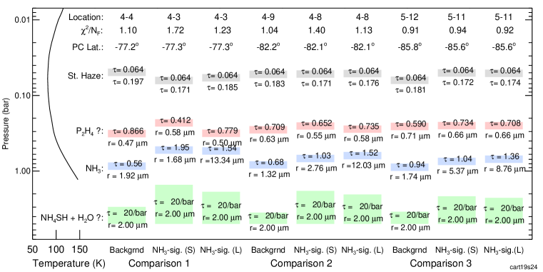
Figure 11.— Comparison of inferred structures of three NH₃-signature clouds with the structures of the nearby background clouds. We show both the small-$r_{3}$ and large-$r_{3}$ solutions for the NH₃-signature clouds, identified in the x-axis labels by (S) and (L) respectively. At the top are ID codes that refer to locations marked in Figs. 4 and 5.

The source of the unique spectral signature is in the upper troposphere, mainly controlled by the optical depth and pressure levels of the diphosphine and ammonia layers. The NH₃-signature clouds have optically thicker and higher NH₃ layers, but generally somewhat less optical depth in the diphosphine layer. The alternate solutions to the NH₃-signature cloud structures are compared with each other and with the nearby background structures in Fig. 11. We see that the large-$r_{3}$ solutions suggest less perturbation of the putative diphosphine layer by the presumed convective pulse that generates the NH₃-signature structure.

4.4. Gas profile results

Besides the aerosol parameters, we also included adjustable parameters to constrain the vertical gas profiles for PH₃ and AsH₃. For PH₃, we made use of three PH₃ absorption bands of differing strengths (near 2.9 $\mu$m, 4.3 $\mu$m, and 4.75 $\mu$m) to try to constrain the main parameters defining its vertical profile: the deep mixing ratio $\alpha_{0}$, the pressure break point $p_{b}$, and the scale height ratio $f$ above the break point. What we found in general was a very loosely constrained pressure break point near the top of the main cloud layer (near 200 mbar) rather than the value of 550 mbar used by Fletcher et al. (2009a), or the 1.3 bar value inferred from VIMS 5-$\mu$m emission spectra by Fletcher et al. (2011). More recent analysis of the VIMS 5-$\mu$m emission spectra by Barstow et al. (2016) found that a break point at 1.1 bars was the best-fit value for nadir-only spectral fits, but was much lower when limb darkened observations were included and might be even lower than 500 mbar, which was the lowest pressure they considered. However, even with our use of daytime observations that allow us to sample three spectral bands of PH₃, there remains such a strong correlation between the spectral effects of a scale height change and those due to a change in pressure break point (as shown in Section 4.5 in Figs. 13 and 14), that these two cannot be independently well constrained. Thus, we chose to fix the scale height ratio at a small value of 0.1 and fit only the other two profile parameters (the deep VMR, and the pressure break point). This relatively sharp drop in PH₃ above the cloud tops is similar to that found by Prinn and Lewis (1975) in their models of PH₃ photolysis in the weakly convective regions on Jupiter.

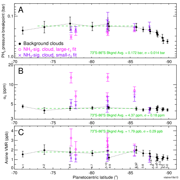
Figure 12.— Retrieved PH₃ break point pressures (A), deep PH₃ mixing ratios (B), and arsine deep mixing ratios (C), all versus planetocentric latitude. Filled circles (black) indicate fits to background cloud models. Fits to spectra of NH₃–signature cloud features are plotted as open circles (magenta) for large-$r_{3}$ solutions and as $\times$’s (purple) for small-$r_{3}$ solutions.

Our gas parameter fit results for background cloud models given in Tables 3 and 4, as well as NH₃-signature cloud fits given in Tables 6 and 7, are all plotted in Fig. 12 as a function of latitude. The parameters derived from background spectra have remarkably smooth variations with latitude, all remaining fairly constant between about 73^∘S and 86^∘S, with averages over that region of 172 mb (with standard deviation of $\sigma$ = 14 mbar) for the PH₃ pressure breakpoint, 4.4 ppm ($\sigma$ = 0.2 ppm) for the deep PH₃ mixing ratio (which remains at essentially the same value to the pole), and 1.8 ppb ($\sigma$ = 0.3 ppb) for the AsH₃ mixing ratio. However, between 86^∘S and the pole, the PH₃ breakpoint pressure increased to 400 mb, while the arsine mixing ratio decreased to about 1.1 ppb, both of which suggest downward motions in this latitude band, as well as that AsH₃ probably is not uniformly mixed, but declines with altitude. In general the break-point is found slightly above the the putative diphosphine cloud, which is consistent with the idea that at large incident angles the photochemical destruction of PH₃ is strongly inhibited below the top cloud level.

Our deep PH₃ VMR values in the polar region are generally at the lower end of the 4-9 ppm range of Fletcher et al. (2008), averaging about 4.4 ppm instead of roughly 6 ppm, and do not show any evidence of their large 8 ppm peak near 82^∘S. Perhaps this should not be too surprising given their different modeling assumptions, namely that of a fixed pressure knee at 550 mbar and an adjustable scale height, as well as the fact that we can make use of the very strong PH₃ band centered at 4.3 $\mu$m, which appears in reflected sunlight.

From about 76^∘S to 86^∘S, our mean arsine VMR (1.79$\pm$0.13 ppb) is between the two values derived by Bézard et al. (1989) of 2.4${}^{+1.4}_{-1.2}$ ppb for the thermal component and 0.39${}^{+0.21}_{-0.13}$ ppb for the reflected solar component. These two values are consistent with a mixing ratio that declines with altitude. Our results are also consistent with the deep value of 1.8${}^{+1.8}_{-0.9}$ ppb inferred by Noll et al. (1989), but somewhat lower than the more global value of 2.2$\pm$0.3 ppb obtained by Fletcher et al. (2011) from VIMS nighttime observations assuming scattering clouds. Given evidence for descending motions in the south polar region, it is not too surprising to find a somewhat reduced level of arsine relative to global mean values. It is also the case that we are probably characterizing cloud properties better by combining thermal and solar reflected light and including scattering by cloud layers, and that may also be a factor in retrieval of different arsine abundances.

The PH₃ results for the NH₃–signature cloud structures are generally more uncertain than those obtained for the background cloud structures, perhaps because the NH₃ absorption feature near 3 $\mu$m interferes somewhat with the 2.9-$\mu$m PH₃ absorption feature and the extra cloud opacity in these structures reduce the visibility of gas absorption features. The gas parameters in these regions also have some consistent deviations, most notably the greatly increased deep mixing ratio of PH₃ found for the large-$r_{3}$ solutions (Fig. 12B), which is accompanied by an increased pressure breakpoint (Fig. 12A). Baines et al. (2018) also found comparably enhanced PH₃ mixing ratios associated with the NH₃–signature clouds in the north polar region. The arsine VMR results for the NH₃–signature structures are also elevated for the large-$r_{3}$ solutions, but somewhat depressed for the small-$r_{3}$ solutions. Much smaller deviations from the background gas parameter solutions are found for the small-$r_{3}$ solutions for the PH₃ parameters. The somewhat better fits obtained from the large-$r_{3}$ solutons suggest that there may be more vertical variation in the PH₃ and AsH₃ gas profiles than are simplified models have assumed. This issue warrants further investigation.

Figure 13.— Logarithmic derivatives of I/F with respect to aerosol model parameters (A-K) and gas parameters (L-O), for the background model (5-10) taken at best fit values given in Table 3. Derivatives are taken with respect to $p_{1}$ (A), $p_{2}$ (B), $p_{3}$ (C), $\tau_{1}$ (D), $\tau_{2}$ (E), $\tau_{3}$ (F), $r_{1}$ (G), $r_{2}$ (H), $r_{3}$ (I), $r_{4}$ (J), $p_{\mathrm{4t}}$ (K), $p_{b}$ (L), $\alpha_{0}$ (M), $f$ (N), and $AsH_{3}v$ (O). The dotted curve in N is the curve in L scaled by -0.16.

4.5. Sensitivity of model spectra to model parameters

The strength of influence on the spectrum of various model parameters, and their correlations, are perhaps most easily understood with the help of logarithmic derivatives, of the form

$$\frac{\partial\log(I(\lambda;x_{1},\cdots,x_{N}))}{\partial\log(x_{i})} = \frac{(1/I)\partial I(\lambda;x_{1},\cdots,x_{N})}{(1/x_{i})\partial x_{i}}$$ (2)

$$= \frac{x_{i}\partial I(\lambda;x_{1},\cdots,x_{N})}{I\partial x_{i}},$$

where $x_{i}$ is any of the model parameters $x_{1},\cdots,x_{N}$, and $I$ is the model spectral radiance for the given set of parameters. The relation also holds if radiance $I$ replaced by reflectivity $I(\lambda;x_{1},\cdots,x_{N})/F(\lambda)$. The middle expression in the above equation is easiest to interpret. It states that the logarithmic derivative is the ratio of the fractional change in $I$ (or $I/F$) to the fractional change in parameter $x_{i}$ that produced it. If the ratio is large, then the parameter will be well constrained by the observed spectrum, unless the spectral ratio for that parameter has a shape similar to that for one of the other parameters, in which case their effects may be difficult to distinguish.

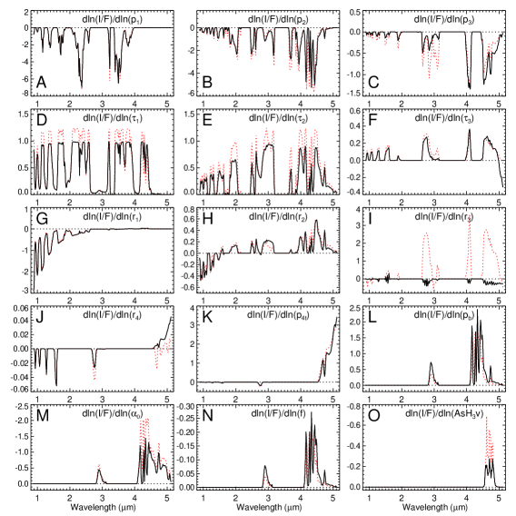
Figure 14.— As in Fig. 13 except that derivatives are taken for the NH₃-signature model (5-9) at best fit parameter values given in Table 6, with results for the large-$r_{3}$ solution in solid black, and for the small-$r_{3}$ solution in dotted red.

Logarithmic derivatives are displayed for the location 5-10 background model structure in Fig. 13 and for the location 5-9 NH₃-signature structures (both large-$r_{3}$ and large-$r_{3}$ solutions) in Fig. 14. Both figures show derivatives for both aerosol parameters (panels A-K) and gas parameters (panels L-O). Note that most derivative spectra are distinctly different from each other, suggesting that most parameters can be well constrained by the observations, if they have sufficient influence on the spectrum. In the aerosol group for NH₃-signature models, the derivatives for $\tau_{3}$ and $r_{3}$ (in panels F and I) are quite similar at wavelengths greater than 2 $\mu$m. However, their influence at shorter wavelengths is very different. Long-exposure VIMS spectra for which the shorter wavelengths are saturated cannot take advantage of this difference, which is one reason we chose not to use them.

A more serious ambiguity appears in the gas parameter group, where panels L and N show extremely similar spectral shapes for derivatives with respect to the phosphine pressure break point (L) and with respect to the phosphine-to-pressure scale height ratio (N). Plotting a scaled version of the former (dotted curve in panel N) on top of the latter’s plot shows that their spectral shapes are nearly indistinguishable. Thus, out of the three parameters used to characterize the vertical distribution of PH₃, only one (the deep phosphine mixing ratio, $\alpha_{0}$) can be constrained well at this model point. This does not mean that there are no boundaries for the other two parameters, only that at the local point where the derivatives are taken, one cannot distinguish between a small fractional increase in the break-point pressure from a small fractional decrease in the phosphine to pressure scale height ratio.

Neither structure allows much sensitivity either to the upper tropospheric VMR of ammonia or its relative humidity. A 100% change in these parameters produces only a few percent fractional change in I/F, which is why we did not try to fit these parameters (or show them in the derivative plots). Also note (in panel K) that increasing the deep layer cloud top pressure has the main effect of increasing the thermal emission (seen at wavelengths beyond 4.5 $\mu$m), although the spectral shapes are different for the two models, due to the much higher pressure for the background model, which provides significantly more visibility of the arsine absorption (evident in panel O). In Fig. 14, the different mixing ratio profiles for phosphine and arsine for the large-$r_{3}$ solution makes their derivatives have less influence on the spectrum.

4.6. Sensitivity of fits to initial guesses

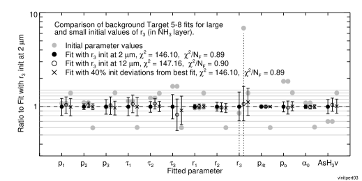
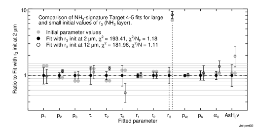
Figure 15.— Effects of different initial values of $r_{3}$ on best fit parameters for a background cloud (top) and an ammonia-signature cloud (bottom). In each panel the grey dots show the initial parameter values, the filled circles the fit that results from a small value for the inital $r_{3}$ value, and the open circles the result for a large guess for the initial $r_{3}$ value. Each parameter is plotted as a ratio to that parameter for the small $r_{3}$ initial value (that is why the first fit results are all on the unit line). For the background example (top) all fitted parameter values for the large-$r_{3}$ guess are nearly identical to the results from the first small-particle fit, well within estimated uncertainties. For the NH₃-signature example (bottom) the ammonia layer parameters and gas mixing ratios are perturbed the most by the new solution obtained.

Physical insight, guided by the logarithmic derivative spectra, was used to formulate manual initial guesses that provide at least crude fits to the observed spectra, which were then refined by our L-M algorithm. To see how sensitive the final results were to the initial crude estimates, we did some trial perturbed calculations, samples of which are illustrated in Fig. 15. The top panel illustrates various fits to the spectrum from location 5-8, which samples a background cloud. Three fits are shown here, with initial guess and best-fit parameter values plotted for each case, shown as ratios to the parameter values obtained from the first fit. The initial guess values for each case are plotted using gray filled circles. The best fit values for the first case are plotted as black dots with error bars. These all have unit central values because they have a unit ratio to themselves. The most uncertain parameter is seen to be the particle radius of the NH₃ cloud layer ($r_{3}$). For the next case, the initial value of that parameter was changed from 2 $\mu$m to 12 $\mu$m. The resulting best fit using that guess, shown by open circles, was very close to the initial fit, with parameter values well within the fitting uncertainties. The next case used an initial guess for each fitted parameter that was either 40% larger or 40% smaller than the best fit value for the first case. Again, the results were almost identical to the initial fit. We conclude that the background fits are not very easily perturbed. It is also worth noting that the parameters best constrained by these fits are r₁, PH₃v, p_4t, p₂, and r₂.

Somewhat different results were obtained from perturbations of fits to the NH₃-signature spectra. In the bottom panel of Fig. 15 we show fit results for such a cloud at location 4-5. The first case uses an inital guess of 2 $\mu$m for $r_{3}$, which settles on $r_{3}$ = 1.75${}^{+0.8}_{-0.5}$ $\mu$m as the best fit, and the second uses an inital guess of 12 $\mu$m for that parameter, yielding the very different best fit value of $r_{3}$ = 14.5$\pm$1.5 $\mu$m. Choosing intermediate first guess values between 2 $\mu$m and 12 $\mu$m resulted in best fit solutions that were close to the original small-$r_{3}$ or large-$r_{3}$ solutions, not to some intermediate value. For the location 4-5 spectrum the large-$r_{3}$ solution actually fits better than the original solution, which is what led us to carry out and present fits with both initial guesses for the NH₃-signature features. This second solution is also seen to result in a somewhat smaller optical depth for the ammonia layer, a larger optical depth for the putative diphosphine layer, and larger values for the two gas mixing ratios. The remaining parameters are within uncertainties of the initial fit, so that the main features of the vertical structure are very similar for both solutions.

5. Discussion

5.1. Vertical structure in the “eyewall” regions.

Shadow measurements by Dyudina et al. (2009) led to the concept of inner and outer eyewalls, each casting shadows on interior cloud regions. One interpretation of these results is illustrated in the right panel of Fig. 3, which displays a stair-step of cloud levels, with each step matching the height of the obstruction needed to cast a shadow of the observed length on a flat region interior to the obstruction. However, as can be seen from cloud structure models displayed in Fig. 9, our radiative transfer modeling provides no corroborating evidence for such large changes of cloud elevation with latitude, nor of any structures with large optical depths that would be expected for eyewall clouds. Thus, it at first appears perplexing that the observed shadows even exist. However, a detailed investigation of the structure of these layers suggests an explanation: small step changes in optical depth versus latitude in the somewhat translucent layers above the ammonia layer can produce shadows on the underlying layer. This mechanism and others are evaluated in a companion paper (Sromovsky et al. 2019), which concludes that it is the only one plausibly consistent with the observations. Here we present evidence for the existence of sharp optical depth transisions that can make that mechanism work.

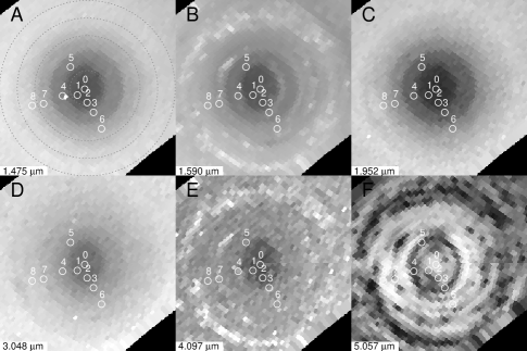
Figure 16.— Polar projection images identifying locations of background spectral samples obtained from VIMS cube V1539288419. For these images the subsolar and sub-spacecraft longitudes are at 178.9^∘E and 149.9^∘E respectively, which are clockwise angles from a horizontal line extending from the pole to the right.

To model the different latitude bands in the inner and outer eye regions, we selected nine spectral samples: three in the darkest inner region, three in the next region between the two shadow boundaries, two just outside the outer shadow, and one in the outer region. The locations of these spectral samples on selected polar projection images are shown in Fig. 16. Note that they all avoid the NH₃-signature features. These sample locations are the same as shown in Fig. 5, and labeled with the same numbers. Our model fits for the locations shown in Fig. 16 were already plotted in Fig. 9 and parameter values and uncertainties given in Table 4. However, optical depths presented earlier were given at a wavelength of 2 $\mu$m. It is also useful to convert these optical depths to the 752-nm wavelength at which shadows are observed in ISS images.

Figure 17.— Best-fit parameter values versus latitude for fits to inner polar region, including pressures (A), optical depths at 752 nm (B), and particle sizes (C). Recall that optical depths in all other figures (and tables) are for a reference wavelength of 2 $\mu$m. Vertical arrows are placed at latitudes indicated by step changes in brightness of ISS images displayed in Fig. 18. The possible step changes are indicated by dashed and dotted lines for upper tropospheric and stratospheric layers respectively. The stratospheric haze optical depths are scaled by a factor of 1/2 to avoid overlap.

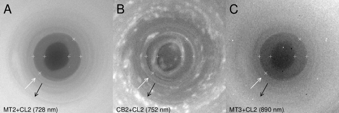
Figure 18.— Polar projections of 2006 ISS images for wavelengths with intermediate (A), low (B), and strong (C) methane gas absorption. Plus signs provide reference marks at identical locations in each image. The direction of incoming sunlight is indicated by white arrows, and direction toward the Cassini spacecraft by the black arrows. Images have been Minnaert corrected to approximately remove limb darkening. Bottom: plots of meridional scans in each image in two directions: horizontal (D) and sun-aligned (E, dotted). Vertical dotted lines are plotted at the same latitudes as the fiducial marks. Arrows in D mark locations of shadow and antishadow features.

The 752-nm optical depths are displayed versus latitude in Fig. 17, which indicate a possible step decrease versus latitude in the optical depth of the stratospheric haze layer might be close to the latitude of the outer “eyewall” shadow and a similar stepped decrease in the optical depth of the putative diphosphine layer may be located near the shadow related to the inner “eyewall”. These step changes, if real, are of roughly the magnitude needed to create shadows on the underlying layer of NH₃ aerosols, i.e. 0.1-0.2 optical depths according to Sromovsky et al. (2019). However, given the relatively large error bars on the fitted optical depth values, the steps are not fully established by our retrievals. Although our radiative transfer analysis shows a decline in optical depth towards the pole, the existence of step changes cannot be firmly inferred from that analysis for two reasons: first, we cannot properly model radiative transfer in close proximity to such a step change because our model relies on the assumption of horizontal homogeneity over a reasonable length scale, and second, the uncertainty in the value of the derived parameters is too large to define a step change over a small spatial region. Our radiative transfer results are consistent with step changes and do constrain the size of the steps, if not their precise shapes.

To confirm the sharpness of these transitions, we used ISS images with up to 8.6 times the spatial resolution of VIMS. The ISS images shown in Fig. 18 illustrate a correlation between features in the upper altitude cloud layers sensed by 728-nm and 890-nm images, and the shadow features that appear in the more deeply sensing 752-nm image. Figure 18 also shows scans along horizontal and sun-aligned meridians in the lower two panels. The ISS 728-nm image senses deeply enough to register sharp changes in both stratospheric and NH₃ layers, but the ISS 890-nm image sees a highly attenuated view due to overlying methane absorption. The scans make clear that the shadows are relatively subtle features of the order of 10% or smaller. The scans also show brightening on the opposite side of the pole, labeled in the figure as antishadows. These arise from extra illumination underneath the layers that cast shadows when they are on the sunward side of the pole, as illustrated by the photographs of a toy physical model displayed in Fig. 19. These bright features cannot be due to light reflected by eyewalls because they are on the wrong side of the boundary that produces shadows when it is on the opposite side of the pole. A more complete and quantitative treatment of this topic is provided by Sromovsky et al. (2019).

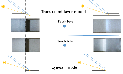
Figure 19.— Photographs of tracing-paper physical models illustrating two alternative shadow production mechanisms: a sharp change in optical depth of a translucent layer (top) or a step change in cloud pressure at an eyewall edge (bottom). Light from the sun is indicated by orange rays, and light to the observer is indicated by blue rays. Each model produces a shadow on the lower layer when the transition is located on the sunward side (left) of the pole. But on the opposite side (right) the translucent layer model displays a moderately bright “antishadow” produced by light shining underneath the top layer and providing extra illumination from below, while the alternate model displays a brightly illuminated eyewall. When illuminated and observed at the angles illustrated here, which are comparable to those for the ISS images in Fig. 18, the antishadow is seen to extend from the upper layer boundary (marked by dashed lines) away from the pole, which is also the direction seen in the ISS images, while the bright eyewall is seen to extend towards the pole, in conflict with ISS observations.

5.2. Making and masking of the NH₃ spectral signature

Figure 20 illustrates how the ammonia signature varies with the vertical level and optical depth of the ammonia layer. The base model in this figure (shown in black) is for the background cloud spectrum from location 4 in Fig. 4. If the top tropospheric layer (the putative diphosphine layer) were instead composed of NH₃, the result would be a sharp and significant spectral feature near 2.986 $\mu$m, as illustrated by the red model spectrum in Fig. 20. There are two reasons that feature is not seen in the base model. First, the NH₃ cloud layer is underneath 0.87 optical depths of the “diphosphine” layer, which is helped in obscuring the feature by the large zenith angles of sun and observer. Second, the NH₃ layer is deep enough that it is affected by overlying phosphine gas absorption, which also obscures the absorption features produced by the cloud particles. The effectiveness of these masking effects is shown by the very small difference between the base model and the model in which the NH₃ layer absorption is turned off by setting n₃ = 1.4 + 0$i$ (orange curve).

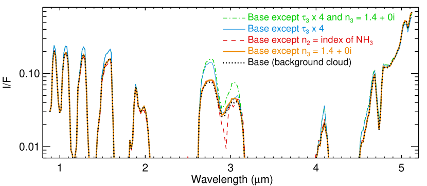
Figure 20.— Model calculations illustrating how the spectral signature of NH₃ is altered by aerosol vertical location and optical depth changes. The base model is background model 5-4 in Table 3. Other curves show the effects of changing layer-3 index (orange) from the normal ammonia index to one with the same real value but without absorption, changing the layer 2 index (red) from its normal real value to the ammonia index, increasing the layer 3 (ammonia layer) optical depth (blue), and increasing the optical depth of layer 3 but removing its ammonia absorption (green).

The effect of NH₃ absorption is more apparent when the overlying layer optical depth is reduced, or when the ammonia layer optical depth is increased. This is shown in Fig. 20 by the blue and green curves. The blue spectrum is computed for the base model except for a factor of 4 increase in the ammonia layer optical depth. The green spectrum is for the same model except that the ammonia absorption is turned off by setting n₃ = 1.4 +0$i$. Without ammonia absorption, the I/F values at 2.7 $\mu$m and 3.1 $\mu$m increase by comparable fractional amounts relative to the base model (black). But with ammonia absorption included, the I/F increase at 3.1 $\mu$m becomes negligible, while the increase at 2.7 $\mu$m remains nearly the same as without ammonia absorption. This shows that the reflectivity of the ammonia cloud at 3.1 $\mu$m becomes saturated because of its low single-scattering albedo.

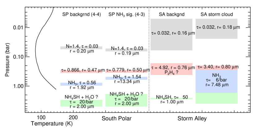
Figure 21.— Vertical cloud structure inferred from fitting background and NH₃ signature cloud spectra (large-$r_{3}$ solution) in comparison with models of the Storm Alley background and storm cloud structures for locations L and H in Fig. 22 of Sromovsky et al. (2018). Note that the derived bottom boundary of the stratospheric haze for the Storm Alley fits is highly uncertain and differences shown here are roughly within uncertainties.

5.3. Comparison of polar clouds to Storm Alley clouds

Here we compare our polar cloud structure models with typical models derived by Sromovsky et al. (2018) for the Storm Alley cloud features. In the left two columns of Fig. 21 is a pair of south polar model fits for an ammonia-signature cloud (at location 4-3) and a background cloud (at location 4-4), and in the right is a pair of Storm Alley fits for background and ammonia-signature storm clouds from Sromovsky et al. (2018). The most striking difference between these models is the large optical depth of the upper tropospheric (pink) layer in the Storm Alley case, both for the background and for the storm cloud. The optical depth for Storm Alley background clouds is nearly six times larger than for the background cloud in the south polar region. For the storm cloud, although the optical depth of that layer is reduced, its ratio to ammonia-signature polar clouds is more than a factor of four. In Storm Alley, producing an ammonia signature requires significant penetration of ammonia ice particles into the overlying putative diphosphine layer, while in the south polar region the upper tropospheric layer has such a low optical depth that relatively small increases in the ammonia layer opacity or decreases in the upper layer opacity can produce the signature. There is a caveat regarding the optical depth of the putative diphosphine layer in the Storm Alley background cloud structure. The Sromovsky et al. (2018) fit to that structure did not include a potential NH₃ ice particle layer. It is likely the case that the 4.9 optical depths of the diphosphine layer could be split roughly equally between an upper layer of diphosphine particles and a lower layer of NH₃ particles. With that much optical depth, it would be hard to distinguish the two configurations.

5.4. The structure of polar dark spots

There are two prominent dark features in Fig. 4 that are darker than background clouds over a wide range of continuum and pseudo-continuum wavelengths. One appears at the upper left and a second can be seen near the bottom, intersecting the left edge of the images. Although we did not conduct a systematic investigation of dark features, we did fit one spectrum from the dark feature near location 4-2. The immediate background structure surrounding this feature is similar to prior fits at similar latitudes. The main difference in the structure of the dark feature itself was found in the ammonia layer, which had a low optical depth of 0.54$\pm$0.18, while the nearby background cloud had a rather normal ammonia layer optical depth of 0.98$\pm$0.17. These dark features merit further investigation to search for possible clues about the dynamical mechanisms that might create them.

6. Summary and Conclusions

We were able to accurately model VIMS near-IR spectra of the south polar region, sampling background clouds from 71^∘S to nearly 90^∘S, and NH₃–signature features from 77.3^∘S to 87.5^∘S, using a four-layer aerosol model, each with different scattering properties and composition: a stratospheric haze, assumed conservative at n = 1.4 at near-IR wavelengths, a putative diphosine cloud, an ammonia ice cloud layer, and a deep diffuse cloud assumed to extend from 5 bars upward to an adjustable pressure, which is in the region where NH₄SH and H₂O are likely condensibles. All layers were characterized as spherical particles. The top three layers were characterized by fitted particle radius, pressure, and optical depth, and given a small physical thickness, making them essentially sheet clouds. We also fit PH₃ and AsH₃ gas mixing ratios. Our analysis of Cassini/VIMS spectra of the south polar region of Saturn have led to the following conclusions.

Background structure. The top three layers have typical fitted pressures of 50 mbar, 320 mbar, and 980 mbar, with corresponding particle radii of 0.19 $\mu$m, 0.6 $\mu$m, and 1.6 $\mu$m, and 2-$\mu$m optical depths of 0.023, 0.72, and 0.80, respectively. The optical depth increases of the stratospheric haze increases are a factor of 20 larger at 752 nm, making the stratospheric haze as impactful as the upper tropospheric layer in possible creation of shadows on the underlying NH₃ layer, the composition of which is confirmed by the detection of its 2.9-3.1 $\mu$m absorption feature. As the pole is approached, the stratospheric haze (layer 1) optical depth decreases by a factor of 2 near 88^∘N and the putative diphosphine haze (layer 2) decreases by about 30% near 89^∘N.

NH₃-signature structures. In these structures the tops of the deep layer are all elevated by about 1 bar (higher in altitude) relative to the same layer in the typical background cloud structure, and the ammonia layer relative to its properties in background regions is typically elevated by about 200 mb, increased in optical depth by as much as 100%, and increased in particle size (significantly for the large-$r_{3}$ solutions). This suggests that deep convection, perhaps in the water layer, is involved in generating the observed differences in the NH₃ layers, although there is no evidence of vertical mass transport from deep levels to the visible cloud deck, as there is for the Great Storm of 2010-2011. However, this might be an approximate realization of the Taylor-Proudman theorem, in which an upward convective pulse at the 2-3 bar level could force the entire column above that pulse to move upward, inducing a pulse of condensation at lower pressures, more evident in the ammonia layer than in the putative diphosphine layer.

Why penetrating convection is not needed to see NH₃ signatures. The 3-$\mu$m absorption is more apparent in the polar region due to the reduced optical depth of the upper cloud layer (the putative diphosphine layer), which can be an order of magnitude smaller than in other regions on Saturn, perhaps because of polar downwelling or reduced rates of photochemical production, or some combination of both.

Lack of evidence for eyewalls. The cloud structures inferred from our radiative transfer modeling are not consistent with the south polar cloud structure suggested by the results of Dyudina et al. (2009). None of the modeled cloud layers disappear, and their optical depths are relatively small and do not change dramatically with latitude. There is no evidence for an optically thick vertical wall of clouds as found in hurricanes on earth, and no detection of lightning.

Alternative shadow mechanism: step changes in optical depths of translucent layers. From ISS imaging at 728 nm, which can detect the top two layers of our model, but not the ammonia layer, it is clear that the optical depth changes noted above probably occur in sharp steps, one at 2^∘ from the pole, and a second near 1.2^∘ from the pole. As confirmed by a simplified Monte Carlo analysis presented in our companion paper (Sromovsky et al. 2019), these optical depth transitions are probably large enough and sharp enough to produce shadows and antishadows of roughly the observed magnitudes.

Existence of antishadows supports the alternative mechanism. The observations of bright features emanating from the same horizontal aerosol boundaries as shadows, but seen on opposite sides of the pole, can arise from extra sunlight shining underneath a layer due to lower optical depth on the sunward side of the layer, producing what we call antishadows. For the VIMS and ISS observing geometry, these features extend away from the pole, while illuminated eyewalls would be seen as bright features extending toward the pole, the opposite of what is observed on Saturn. This provides additional strong evidence that step changes in physically thin overlying layers are the source of shadows.

Phosphine. From fitting models to background clouds, there seems to be a fairly latitude independent deep mixing ratio, with an average of 4.33$\pm$0.05 ppm, and a peak-to-peak range of 4.1-4.7 ppm. However, we found a significant increase in the break-point pressure from about 200 mbar near 86^∘S to 400 mbar at 89.8^∘S. This result seems at least qualitatively consistent with the polar decline within 2^∘ of the south pole that was found by Fletcher et al. (2008), although our different modeling approach makes direct comparisons uncertain. Fitting of NH₃-signature structures suggests that the PH₃ mixing ratios are locally increased by factors of 2-3 over background values and that pressure break points in those regions also seem to be generally increased.

Arsine. From background fits it appears that south polar arsine volume mixing ratios are relatively latitude independent between 77^∘S and 86^∘S, over which the average value was found to be 1.71$\pm$0.13 ppb. From 86^∘to the pole the mixing ratio declines to 1.1$\pm$0.2 ppb. This suggests that arsine’s mixing ratio declines with altitude, as suggested previously by results of Bézard et al. (1989), such that descending motions near the pole produce a lower effective mixing ratio. For NH₃-signature fits we find somewhat decreased mixing ratios for the small-$r_{3}$ solutions, but the opposite for the large-$r_{3}$ solutions.

There are more than a few questions to be resolved about the south polar cloud structure of Saturn. The composition of the ubiquitous upper tropospheric layer seems likely to be either diphosphine or phosphorus. But to test which better fits spectral observations, we need better measurements of the optical properties of both of these materials under Saturnian conditions, especially of diphosphine about which very little is known. There is also a caveat that must be recognized in the modeling of the discrete bright features. These are probably affected to at least a small degree by the violation of the assumption of horizontal homogeneity, as many of these features are of the same horizontal scale as the vertical distance between cloud layers. Furthermore, it must be noted that these results are based on one snapshot taken in 2006. Temporal evolution of the south polar cloud structure is also uncertain because of the scarcity of observations of adequate spatial resolution. However, based on analysis of HST observations by Pérez-Hoyos et al. (2005) there is some evidence that optical depths at 80^∘S and 86^∘S may have declined significantly in the several years prior to the 2003 southern solstice. If and when they begin to increase remains to be determined.

References

- Acton (1996) Acton, C. H., 1996. Ancillary data services of NASA’s Navigation and Ancillary Information Facility. Planet. and Space Sci. 44, 65–70.
- Anderson et al. (2004) Anderson, J. A., Sides, S. C., Soltesz, D. L., Sucharski, T. L., Becker, K. J., 2004. Modernization of the Integrated Software for Imagers and Spectrometers. In: Mackwell, S., Stansbery, E. (Eds.), Lunar and Planetary Science Conference. Vol. 35 of Lunar and Planetary Science Conference. p. 2039.
- Atreya and Wong (2005) Atreya, S. K., Wong, A., 2005. Coupled Clouds and Chemistry of the Giant Planets - A Case for Multiprobes. Space Sci. Rev. 116, 121–136.
- Baines et al. (2009) Baines, K. H., Delitsky, M. L., Momary, T. W., Brown, R. H., Buratti, B. J., Clark, R. N., Nicholson, P. D., 2009. Storm clouds on Saturn: Lightning-induced chemistry and associated materials consistent with Cassini/VIMS spectra. Planet. & Space Sci.57, 1650–1658.
- Baines et al. (2008) Baines, K. H., Momary, T. W., Kim, J. H., Roos-Serote, M., Showman, A. P., Atreya, S. K., Brown, R. H., Buratti, B. J., Clark, R. N., Nicholson, P. D., 2008. Saturn’s dynamic atmosphere at depth: Physical characteristics, winds, and spatial constraints on trace gas variability near the 3-bar level and their dynamical implications from Cassini-Hygens/VIMS. In: Poster Presented at Saturn after Cassini Huygens Conference, Imperial College, London.
- Baines et al. (2018) Baines, K. H., Sromovsky, L. A., Fry, P. M., Momary, T. W., Brown, R. H., Buratti, B. J., Clark, R. N., Nicholson, P. D., Sotin, C., 2018. The Eye of Saturn’s North Polar Vortex: Unexpected Cloud Structures Observed at High Spatial Resolution by Cassini/VIMS. Geophys. Res. Let.45, 5867–5875.
- Barstow et al. (2016) Barstow, J. K., Irwin, P. G. J., Fletcher, L. N., Giles, R. S., Merlet, C., 2016. Probing Saturn’s tropospheric cloud with Cassini/VIMS. Icarus 271, 400–417.
- Bézard et al. (1989) Bézard, B., Drossart, P., Lellouch, E., Tarrago, G., Maillard, J. P., 1989. Detection of arsine in Saturn. Astrophys. J.346, 509–513.
- Borysow (1991) Borysow, A., 1991. Modeling of collision-induced infrared absorption spectra of H2-H2 pairs in the fundamental band at temperatures from 20 to 300 K. Icarus 92, 273–279.
- Borysow (1992) Borysow, A., 1992. New model of collision-induced infrared absorption spectra of H2-He pairs in the 2-2.5 micron range at temperatures from 20 to 300 K - an update. Icarus 96, 169–175.
- Borysow (1993) Borysow, A., 1993. Erratum. Icarus 106, 614.
- Bowles et al. (2008) Bowles, N., Calcutt, S., Irwin, P., Temple, J., 2008. Band parameters for self-broadened ammonia gas in the range 0.74 to 5.24 m to support measurements of the atmosphere of the planet Jupiter. Icarus 196, 612–624.
- Briggs and Sackett (1989) Briggs, F. H., Sackett, P. D., 1989. Radio observations of Saturn as a probe of its atmosphere and cloud structure. Icarus 80, 77–103.
- Brown et al. (2004) Brown, R. H., Baines, K. H., Bellucci, G., Bibring, J.-P., Buratti, B. J., Capaccioni, F., Cerroni, P., Clark, R. N., Coradini, A., Cruikshank, D. P., Drossart, P., Formisano, V., Jaumann, R., Langevin, Y., Matson, D. L., McCord, T. B., Mennella, V., Miller, E., Nelson, R. M., Nicholson, P. D., Sicardy, B., Sotin, C., 2004. The Cassini Visual and Infrared Mapping Spectrometer (VIMS) Investigation. Space Sci. Rev. 115, 111–168.
- Clapp and Miller (1996) Clapp, M. L., Miller, R. E., 1996. Complex Refractive Indices of Crystalline Hydrazine from Aerosol Extinction Spectra. Icarus 123, 396–403.
- Clark et al. (2012) Clark, R. N., Cruikshank, D. P., Jaumann, R., Brown, R. H., Stephan, K., Dalle Ore, C. M., Eric Livo, K., Pearson, N., Curchin, J. M., Hoefen, T. M., Buratti, B. J., Filacchione, G., Baines, K. H., Nicholson, P. D., 2012. The surface composition of Iapetus: Mapping results from Cassini VIMS. Icarus 218, 831–860.
- Drummond and Thekaekara (1973) Drummond, A., Thekaekara, M., 1973. The extraterrestrial solar spectrum. Institute of Environmental Sciences, Mt. Prospect Illinois.
- Dyudina et al. (2009) Dyudina, U. A., Ingersoll, A. P., Ewald, S. P., Vasavada, A. R., West, R. A., Baines, K. H., Momary, T. W., Del Genio, A. D., Barbara, J. M., Porco, C. C., Achterberg, R. K., Flasar, F. M., Simon-Miller, A. A., Fletcher, L. N., 2009. Saturn’s south polar vortex compared to other large vortices in the Solar System. Icarus 202, 240–248.
- Dyudina et al. (2008) Dyudina, U. A., Ingersoll, A. P., Ewald, S. P., Vasavada, A. R., West, R. A., Del Genio, A. D., Barbara, J. M., Porco, C. C., Achterberg, R. K., Flasar, F. M., Simon-Miller, A. A., Fletcher, L. N., 2008. Dynamics of Saturn’s South Polar Vortex. Science 319, 1801.
- Fletcher et al. (2011) Fletcher, L. N., Baines, K. H., Momary, T. M., Showman, A. S., Irwin, P. G. J., Orton, G. S., Roose-Serote, M. R., Merlit, C., 2011. Saturn’s tropospheric composition and clouds from Cassini/VIMS 4.6 – 5.1 m nightside spectroscopy. Icarus 214, 510–533.
- Fletcher et al. (2008) Fletcher, L. N., Irwin, P. G. J., Orton, G. S., Teanby, N. A., Achterberg, R. K., Bjoraker, G. L., Read, P. L., Simon-Miller, A. A., Howett, C., de Kok, R., Bowles, N., Calcutt, S. B., Hesman, B., Flasar, F. M., 2008. Temperature and Composition of Saturn’s Polar Hot Spots and Hexagon. Science 319, 79.
- Fletcher et al. (2009a) Fletcher, L. N., Orton, G. S., Teanby, N. A., Irwin, P. G. J., 2009a. Phosphine on Jupiter and Saturn from Cassini/CIRS. Icarus 202, 543–564.
- Fletcher et al. (2009b) Fletcher, L. N., Orton, G. S., Teanby, N. A., Irwin, P. G. J., Bjoraker, G. L., 2009b. Methane and its isotopologues on Saturn from Cassini/CIRS observations. Icarus 199, 351–367.
- Fouchet et al. (2009) Fouchet, T., Moses, J. I., Conrath, B. J., 2009. Saturn: Composition and Chemistry. In: Dougherty, M. K., Esposito, L. W., Krimigis, S. M. (Eds.), Saturn from Cassini-Huygens. Springer Dordrecht Heidelberg London New York, pp. 83–112.
- Frankiss (1968) Frankiss, S. G., 1968. Vibrational Spectrum and Structure of Solid Diphosphine. Inorg. Chem. 7, 1931–1933.
- Hansen and Travis (1974) Hansen, J. E., Travis, L. D., 1974. Light scattering in planetary atmospheres. Space Sci. Rev. 16, 527–610.
- Hide (1966) Hide, R., 1966. On the circulation of the atmospheres of Jupiter and Saturn. Planet. & Space Sci.14, 669.
- Howett et al. (2007) Howett, C. J. A., Carlson, R. W., Irwin, P. G. J., Calcutt, S. B., 2007. Optical constants of ammonium hydrosulfide ice and ammonia ice. Journal of the Optical Society of America B Optical Physics 24, 126–136.
- Karkoschka and Tomasko (2010) Karkoschka, E., Tomasko, M. G., 2010. Methane absorption coefficients for the jovian planets from laboratory, Huygens, and HST data. Icarus 205, 674–694.
- Lindal et al. (1985) Lindal, G. F., Sweetnam, D. N., Eshleman, V. R., 1985. The atmosphere of Saturn - an analysis of the Voyager radio occultation measurements. Astron. J.90, 1136–1146.
- Martonchik et al. (1984) Martonchik, J. V., Orton, G. S., Appleby, J. F., 1984. Optical properties of NH3 ice from the far infrared to the near ultraviolet. Appl. Optics 23, 541–547.
- Miller et al. (1996) Miller, E. A., Klein, G., Juergens, D. W., Mehaffey, K., Oseas, J. M., Garcia, R. A., Giandomenico, A., Irigoyen, R. E., Hickok, R., Rosing, D., Sobel, H. R., Bruce, C. F., Flamini, E., Devidi, R., Reininger, F. M., Dami, M., Soufflot, A., Langevin, Y., Huntzinger, G., 1996. The Visual and Infrared Mapping Spectrometer for Cassini. In: Horn, L. (Ed.), Society of Photo-Optical Instrumentation Engineers (SPIE) Conference Series. Vol. 2803. pp. 206–220.
- Nixon (1956) Nixon, E. R., 1956. The Infrared Spectrum of Biphosphine. J. Phys. Chem. 60, 1054–1059.
- Noll et al. (1989) Noll, K. S., Geballe, T. R., Knacke, R. F., 1989. Arsine in Saturn and Jupiter. Astrophys. J. Lett.338, L71–L74.
- Noy et al. (1981) Noy, N., Podolak, M., Bar-Nun, A., 1981. Photochemistry of phosphine and Jupiter’s Great Red Spot. J. Geophys. Res. 86, 11985–11988.
- Pedlosky (1982) Pedlosky, J., 1982. Geophysical fluid dynamics. New York and Berlin, Springer-Verlag, 1982. 636 p.
- Pérez-Hoyos et al. (2005) Pérez-Hoyos, S., Sánchez-Lavega, A., French, R. G., Rojas, J. F., 2005. Saturn’s cloud structure and temporal evolution from ten years of Hubble Space Telescope images (1994 – 2003). Icarus 176, 155–174.
- Pérez-Hoyos et al. (2016) Pérez-Hoyos, S., Sanz-Requena, J. F., Sánchez-Lavega, A., Irwin, P. G. J., Smith, A., 2016. Saturn’s tropospheric particles phase function and spatial distribution from Cassini ISS 2010-11 observations. Icarus 277, 1–18.
- Porco et al. (2004) Porco, C. C., West, R. A., Squyres, S., McEwen, A., Thomas, P., Murray, C. D., Delgenio, A., Ingersoll, A. P., Johnson, T. V., Neukum, G., Veverka, J., Dones, L., Brahic, A., Burns, J. A., Haemmerle, V., Knowles, B., Dawson, D., Roatsch, T., Beurle, K., Owen, W., 2004. Cassini Imaging Science: Instrument Characteristics and Anticipated Scientific Investigations at Saturn. Space Science Reviews 115, 363–497.
- Press et al. (1992) Press, W. H., Teukolsky, S. A., Vetterling, W. T., Flannery, B. P., 1992. Numerical recipes in FORTRAN. The art of scientific computing, 2nd ed. Cambridge: University Press.
- Prinn and Lewis (1975) Prinn, R. G., Lewis, J. S., 1975. Phosphine on Jupiter and implications for the Great Red Spot. Science 190, 274–276.
- Roux et al. (1979) Roux, J. A., Wood, B. E., Smith, A. M., 1979. Optical properties of thin H20, NH3, and CO2 cryofilms. AEDC-TR-79-57. Arnold Engineering Development Center, Tennessee.
- Sromovsky et al. (2013) Sromovsky, L. A., Baines, K. H., Fry, P. M., 2013. Saturn’s Great Storm of 2010-2011: Evidence for ammonia and water ices from analysis of VIMS spectra. Icarus 226, 402–418.
- Sromovsky et al. (2018) Sromovsky, L. A., Baines, K. H., Fry, P. M., 2018. Models of bright storm clouds and related dark ovals in Saturn’s Storm Alley as constrained by 2008 Cassini/VIMS spectra. Icarus 302, 360–385.
- Sromovsky et al. (2016) Sromovsky, L. A., Baines, K. H., Fry, P. M., Momary, T. W., 2016. Cloud clearing in the wake of Saturn’s Great Storm of 2010-2011 and suggested new constraints on Saturn’s He/H2 ratio. Icarus 276, 141–162.
- Sromovsky and Fry (2010) Sromovsky, L. A., Fry, P. M., 2010. The source of 3-m absorption in Jupiter’s clouds: Reanalysis of ISO observations using new NH3 absorption models. Icarus 210, 211–229.
- Sromovsky et al. (2019) Sromovsky, L. A., Fry, P. M., Baines, K. H., 2019. Interpretation of south polar cloud shadows and antishadows on Saturn. Icarus, submitted.
- Sromovsky et al. (2012) Sromovsky, L. A., Fry, P. M., Boudon, V., Campargue, A., Nikitin, A., 2012. Comparison of line-by-line and band models of near-IR methane absorption applied to outer planet atmospheres. Icarus 218, 1–23.
- Visscher et al. (2009) Visscher, C., Sperier, A. D., Moses, J. I., Keane, T. C., 2009. Phosphine and Ammonia Photochemistry in Jupiter’s Troposphere. In: Lunar and Planetary Science Conference. Vol. 40 of Lunar and Planetary Science Conference. p. 1201.
- Warren (1984) Warren, S. G., 1984. Optical constants of ice from the ultraviolet to the microwave. Appl. Optics 23, 1206–1225.
- Weidenschilling and Lewis (1973) Weidenschilling, S. J., Lewis, J. S., 1973. Atmospheric and cloud structures of the jovian planets. Icarus 20, 465–476.
- Wohlfarth (2008) Wohlfarth, C., 2008. Refractive index of diphosphine: Datasheet from landolt-börnstein - group iii condensed matter · volume 47: “refractive indices of pure liquids and binary liquid mixtures (supplement to iii/38)” in springermaterials). Copyright 2008 Springer-Verlag Berlin Heidelberg.
- Zheng and Borysow (1995) Zheng, C., Borysow, A., 1995. Modeling of collision-induced infrared absorption spectra of H2 pairs in the first overtone band at temperatures from 20 to 500 K. Icarus 113, 84–90.