IIB flux non-commutativity
and the global structure of field theories

Abstract

We discuss the origin of the choice of global structure for six dimensional $(2,0)$ theories and their compactifications in terms of their realization from IIB string theory on ALE spaces. We find that the ambiguity in the choice of global structure on the field theory side can be traced back to a subtle effect that needs to be taken into account when specifying boundary conditions at infinity in the IIB orbifold, namely the known non-commutativity of RR fluxes in spaces with torsion. As an example, we show how the classification of $\mathcal{N}=4$ theories by Aharony, Seiberg and Tachikawa can be understood in terms of choices of boundary conditions for RR fields in IIB. Along the way we encounter a formula for the fractional instanton number of $\mathcal{N}=4$ ADE theories in terms of the torsional linking pairing for rational homology spheres. We also consider six-dimensional $(1,0)$ theories, clarifying the rules for determining commutators of flux operators for discrete 2-form symmetries. Finally, we analyze the issue of global structure for four dimensional theories in the presence of duality defects.

1 Introduction

One of the fundamental observables that we can use to characterize Quantum Field Theories is their partition function on arbitrary manifolds $\mathcal{M}$. The partition function depends both on intrinsic data $\mathcal{T}$ defining the theory — which we can provide without reference to the underlying manifold — and on background data on $\mathcal{M}$, such as a metric $g_{\mu\nu}$, a Spin connection $\omega^{ab}_{\mu}$, and backgrounds $A_{\mu}$ for the global symmetries of the theory, which might be continuous or discrete. If $\mathcal{M}$ is non-compact, we need to specify boundary conditions for the theory, which we denote as $\left|\psi\right\rangle$, for reasons that will become apparent momentarily. For a theory $\mathcal{T}$ on a manifold $\mathcal{M}$ with this structure specified, we can thus write

$$Z_{\mathcal{T}}[\mathcal{M}(g,\omega,A,\left|\psi\right\rangle)]$$ (1)

for the partition function.

Our main interest in this paper will be the case in which $\mathcal{T}$ is a six-dimensional SCFT preserving $\mathcal{N}=(2,0)$ supersymmetry, which we construct as follows. Consider IIB string theory on a manifold $\mathcal{M}_{6}\times\mathbb{C}^{2}/\Gamma$, with $\Gamma\subset SU(2)$. By the McKay correspondence McKay , the relevant discrete groups $\Gamma$ are in a one-to-one correspondence with the simple Lie algebras of ADE type. Given such an algebra $\mathfrak{g}_{\Gamma}$, we denote by $G_{\Gamma}$ the simply connected Lie group with algebra $\mathfrak{g}_{\Gamma}$. It is a well supported conjecture that this system has a non-trivial interacting fixed point at low energies, given by an interacting six-dimensional $\mathcal{N}=(2,0)$ SCFT Witten:1995zh , known as the $(2,0)$ theory of type $\mathfrak{g}_{\Gamma}$. In fact, all known interacting $(2,0)$ SCFTs that do not factorize into decoupled SCFTs at the level of local operators can be obtained from this construction.

The $(2,0)$ theory of type $\mathfrak{g}_{\Gamma}$ has a number of remarkable properties, one of the most exotic ones being that on generic $\mathcal{M}_{6}$ there is no canonical choice for the background connection for its global symmetries. More concretely, the $(2,0)$ theory of type $\mathfrak{g}_{\Gamma}$ is believed to possess a discrete global 2-form symmetry Gaiotto:2014kfa given by the center $Z(G_{\Gamma})$ of $G_{\Gamma}$. The generators of this symmetry do not all commute with each other, so quantum mechanically there is no way of setting all background fields for the 2-form symmetry to zero. The following consequence of this fact might be more familiar: upon compactification on $T^{2}$ the $(2,0)$ theory becomes $\mathcal{N}=4$ SYM with gauge algebra $\mathfrak{g}_{\Gamma}$, and the 2-form symmetry gives rise to the 1-form symmetries measuring the number of Wilson and ’t Hooft lines. It is a familiar fact that the associated symmetry generators do not commute THOOFT19781 ; THOOFT1979141 .

Since the symmetry generators do not commute, they are not simultaneous observables. The best we can do is to select a maximal commuting subset of these operators and decompose the Hilbert space in their simultaneous eigenbasis. By selecting an eigenvector from this basis, an associated subset of the background fields for the 2-form symmetry can all be set to zero, or to any definite value. However, choosing a maximal commuting set of fluxes to fix requires explicit reference to the structure of $H^{3}(\mathcal{M}_{6};Z(G_{\Gamma}))$, and generically such a choice will not be invariant under large diffeomorphisms of $\mathcal{M}_{6}$. This can be naturally interpreted as an anomaly (see Monnier:2019ytc for an introduction), but the fact that the ambiguity in the partition function is not just a phase makes the situation exotic. This state of affairs is often described by saying that the $(2,0)$ theory has a partition vector (of “conformal blocks”, in analogy with the situation for chiral theories in two dimensions) as opposed to having a partition function, or sometimes, more concisely, by saying that the $(2,0)$ theory is a “metatheory”.

At this point we reach a puzzle, which this paper aims to clarify: we have explained that generally there is no canonical choice of partition function for the six-dimensional $(2,0)$ theory, due to the non-commutativity of the operators generating the 2-form symmetry. But on the other hand, we started our discussion by saying that the $(2,0)$ theory of type $\mathfrak{g}_{\Gamma}$ can be constructed by considering a low-energy limit of IIB string theory on $\mathbb{C}^{2}/\Gamma\times\mathcal{M}_{6}$. The fact that there is no canonical choice of partition function for the $(2,0)$ theory should then imply that there is no canonical choice for the partition function of IIB string theory on $\mathbb{C}^{2}/\Gamma\times\mathcal{M}_{6}$. We will argue that this is indeed the case.

Briefly, in order to have a well defined partition function of the IIB theory on $\mathbb{C}^{2}/\Gamma\times\mathcal{M}_{6}$ one needs to specify boundary conditions for the RR fluxes, and in the presence of torsion this is a fairly subtle affair due to the self-dual nature of RR fields in string theory Freed:2006ya ; Freed:2006yc . We will show that there is indeed no choice of boundary conditions in which all RR fluxes are set to zero at infinity, and in fact the set of choices for boundary conditions for IIB on $\mathbb{C}^{2}/\Gamma\times\mathcal{M}_{6}$ is in one-to-one correspondence with the set of choices one makes in choosing a partition function for the $(2,0)$ theory of type $\mathfrak{g}_{\Gamma}$ on $\mathcal{M}_{6}$.

This result removes a fair bit of mystery from the usual statement that the $(2,0)$ theory has no well-defined partition function, since the standard construction of such theories in string theory requires one to provide the missing data in the form of boundary values for the RR fluxes. Remarkably, all possible choices for the $(2,0)$ theory can be accommodated in the IIB construction. In terms of symmetries our viewpoint provides a reinterpretation of the 2-form symmetry of the $(2,0)$ theory in terms of transformations of the boundary conditions on IIB.

This whole discussion might come as a bit of a surprise to the reader familiar with the proof in Witten:1996hc ; Witten:1999vg that there is a canonical partition function of IIB on a ten-manifold $\mathcal{M}_{10}$. The key assumption in the argument in Witten:1996hc ; Witten:1999vg that does not hold for the geometries analyzed in this paper is that $\mathcal{M}_{10}$ has an intersection form with unit determinant. This is always the case for compact manifolds, but generically it is not the case for $\mathcal{M}_{10}=\mathcal{M}_{6}\times\mathbb{C}^{2}/\Gamma$ (except for the case associated with $E_{8}$). Similarly, the statement that string theory always gives rise to modular invariant theories (see for example Seiberg:2011dr ) is true under the assumption that we have a compact transverse space, so that the six-dimensional effective theory of interest is coupled to six-dimensional gravity. But this does not hold for the configurations that we study in this paper, in which the metric is just a background field in the six-dimensional theory. The effective six-dimensional theories that one finds in the case $\mathcal{M}_{10}=\mathcal{M}_{6}\times\mathbb{C}^{2}/\Gamma$ are not modular invariant, but since six-dimensional gravity is non-dynamical there is no contradiction. (The ten-dimensional gravity theory is dynamical, but again there is no contradiction because as we will describe the lack of modular invariance of the six-dimensional theory ultimately comes from the lack of modular invariance of the choice of boundary conditions on $\mathcal{M}_{6}\times S^{3}/\Gamma$, and we do not sum over these when doing the gravitational path integral.)

We emphasize that our viewpoint here, focusing purely on a careful analysis of the original construction of $(2,0)$ theories in ten dimensional type IIB string theory, is complementary to existing viewpoints on the partition function of $(2,0)$ theories. One such viewpoint is that of relative QFTs articulated by Freed and Teleman in Freed:2012bs , where one views the $(2,0)$ theories as furnishing the boundary degrees of freedom for certain non-invertible seven dimensional TQFTs Monnier:2014txa ; Monnier:2016jlo ; Monnier:2017klz . For the $A_{N}$ cases one can also study the question using holography Witten:1998wy . We find that all three approaches give the same results whenever they are simultaneously applicable.

We have organized this paper as follows. We start in §2 by explaining how to choose boundary condition for RR fields in IIB string theory on $\mathcal{M}_{6}\times\mathbb{C}^{2}/\Gamma$. In §3 we compare the results of §2 to the known results for the behaviour of the $(2,0)$ partition function, and extend the results to the $(1,0)$ case, refining a previous proposal in DelZotto:2015isa . We then show how one can rederive the known classification of four dimensional $\mathcal{N}=4$ theories Aharony:2013hda (of ADE type) from the IIB perspective. Along the way we encounter a simple geometric reinterpretation of the fractional instanton number in $\mathcal{N}=4$ theories with simply-connected gauge group, which we expect to generalize to less supersymmetric cases. In §4 we explore these ideas in less familiar backgrounds: we will discuss global aspects of 4d theories in the presence of duality defects (as studied in Harvey:2007ab ; Cvetic:2011gp ; Martucci:2014ema ; Gadde:2014wma ; Assel:2016wcr ; Choi:2017kxf ; Lawrie:2018jut ; Lawrie:2016axq , for instance) and subtleties having to do with modular invariance in the context of 4d/2d dualities that arise when the four dimensional manifold has two-cycles. We point out an interesting relation between the Vafa-Witten partition function of self-dual $\mathfrak{su}(p)$ theories on $\mathrm{K3}$ and Hecke operators acting on the partition function of chiral bosons, and briefly discuss a (speculative, but suggestive) connection between these partition functions and the $j$ invariant. In §5, we conclude and list a number of directions for further research. Appendix A contains technical results on the complex K-theory groups of rational homology spheres used in the main text, and appendix B discusses the Vafa-Witten partition functions Vafa:1994tf of $\mathcal{N}=4$ theories with algebra $\mathfrak{su}(N)$ on $\mathrm{K3}$ for different choices of the global form of the gauge group, and how their behavior under dualities agrees with expectations.

2 Quantization of type IIB string theory on $\mathcal{M}_{6}\times\mathbb{C}^{2}/\Gamma$

We begin with a short informal outline of the main argument in this section, without going into the technical details. Most of the work in the rest of the section will be in making these arguments fully precise.

Consider type IIB string theory compactified on $\mathcal{M}_{6}\times\mathbb{C}^{2}/\mathbb{Z}_{N}$, which is believed to yield the $A_{N-1}$ $(2,0)$ theory on $\mathcal{M}_{6}$ at low energies. Without changing the behaviour at infinity, we could instead consider a resolution of the $\mathbb{C}^{2}/\mathbb{Z}_{N}$ orbifold, so that the spacetime curvature is arbitrarily small and the string coupling is small and constant. Thus, the subtlety in specifying boundary conditions cannot be due to any particular property of string theory in singular spaces. Instead, it is due to the presence of the self-dual RR field $F_{5}=\ast F_{5}$ in type IIB supergravity. As pointed out in beautiful work by Freed, Moore and Segal Freed:2006ya ; Freed:2006yc (building on Gukov:1998kn ; Moore:2004jv ; Belov:2005ze ; Witten:1998wy ; Belov:2004ht ; Burrington:2006uu ; Burrington:2006aw ; Burrington:2006pu ), quantization of self-dual fields in spaces with torsion needs to be done with care, even at arbitrarily weak coupling.

In more detail, in order to characterize the IIB background we should specify boundary conditions for all the supergravity fields, including $F_{5}$. Classically, we would specify the background value for $F_{5}$ at infinity, which we could simply set to zero if desired. Quantum mechanically, the story is far more subtle. We describe it in detail below, but the main point is that for each class $\sigma\in\operatorname{Tor}(H^{5}(\mathcal{M}_{6}\times S^{3}/\mathbb{Z}_{N};\mathbb{Z}))$ there is a unitary flux operator $\Phi_{\sigma}$, which measures the torsional part of the flux on the homology class Poincaré dual to $\sigma$. The boundary conditions are encoded in the expectation values of these operators, and naively we could simply choose a state with $\left\langle\Phi_{\sigma}\right\rangle=1$ for every $\sigma$, corresponding to a background with no flux at infinity. Surprisingly, this is not possible, as the torsion flux operators for self-dual forms on different cycles do not always commute Freed:2006ya ; Freed:2006yc :

$$\Phi_{\sigma}\Phi_{\sigma^{\prime}}=e^{2\pi i\,\mathsf{L}(\sigma,\sigma^{\prime})}\Phi_{\sigma^{\prime}}\Phi_{\sigma}\,.$$ (2)

Here $\mathsf{L}(\sigma,\sigma^{\prime})$ is the linking pairing for the torsion 5-forms $\sigma,\,\sigma^{\prime}$, taking values in $\mathbb{Q}/\mathbb{Z}$. Most of the technical details in this section deal with the careful computation of this linking pairing.

The nonvanishing commutator (2) implies that one cannot specify the value of all fluxes simultaneously, and in particular one cannot simply set the $F_{5}$ flux to zero at infinity. Instead, the best we can do is to choose a maximal set of commuting flux operators and set the corresponding fluxes to zero (or to another fixed value). Given such a choice we can in principle compute the partition function for type IIB on that background, which also determines the partition function for the $A_{N-1}$ $(2,0)$ theory on $\mathcal{M}_{6}$. However, there is no canonical choice for the maximal subset of commuting operators to set to zero and, in fact, large diffeomorphisms on the boundary typically relate different choices. In light of this, one might expect that the collection of boundary conditions for type IIB in this background, with the subtleties due to non-vanishing commutators properly taken into account, is precisely the vector space of partition functions of the $(2,0)$ theory on $\mathcal{M}_{6}$. In the coming sections we will argue that this expectation is indeed correct.

Note that the RR fields in IIB string theory are more properly described in terms of differential K-theory (see Hopkins:2002rd ; Freed:2000ta ; Freed:2006yc for an introduction). This not only accounts for the local data of the $C_{4}$ connection (the “differential” qualifier), but also the fact that the flux quantization conditions are better described by K-theory Moore:1999gb . However, to understand the commutation relations it is sufficient to restrict to ordinary K-theory, since the commutators depend only on the K-theory class, and more specifically its torsional component. Related to this, the class $\sigma$ really lives in $H^{4}(\mathcal{M}_{6}\times S^{3}/\mathbb{Z}_{n};U(1))$ (or rather, its generalization in differential K-theory) rather than $\operatorname{Tor}(H^{5}(\mathcal{M}_{6}\times S^{3}/\mathbb{Z}_{N};\mathbb{Z}))$, but again to understand the flux commutation relations it will be sufficient to restrict ourselves to torsion classes.

2.1 Flux operators and the Hilbert space $\mathcal{H}^{[RR]}(\mathcal{N}_{9})$

Starting again from the beginning, we aim to specify the boundary conditions for euclidean IIB string theory on a ten-dimensional manifold $X_{10}=\mathcal{M}_{6}\times\mathbb{C}^{2}/\Gamma$, where $\mathcal{M}_{6}$ is closed, oriented, Spin, and without torsion. To understand how to choose boundary conditions properly, we first take a slight detour and review some basic aspects of quantum field theory (see, e.g., HartmanLectures for a less telegraphic exposition).

In general, a $d$-dimensional quantum field theory associates a Hilbert space $\mathcal{H}(\mathcal{N}_{d-1})$ to each $(d-1)$-dimensional manifold $\mathcal{N}_{d-1}$. This Hilbert space is the one associated with quantization of the original theory on $\mathcal{N}_{d-1}\times\mathbb{R}$, where $\mathbb{R}$ denotes the time direction. We stress that we are not yet specifying the value of the fields on $\mathcal{N}_{d-1}$, the Hilbert space only depends on $\mathcal{N}_{d-1}$ itself. Indeed, in the quantum theory a choice of field configuration on $\mathcal{N}_{d-1}$ corresponds to choosing a state $\left|\psi\right\rangle\in\mathcal{H}(\mathcal{N}_{d-1})$.

Now consider the quantum field theory on a manifold $X_{d}$ with boundary $\mathcal{N}_{d-1}=\partial X_{d}$. Then the path integral on $X_{d}$, without specifying the boundary conditions, can be understood as a dual vector $\left\langle Z\right|\in\mathcal{H}^{*}(\mathcal{N}_{d-1})$, so the value of the path integral with boundary conditions specified by $\left|\psi\right\rangle\in\mathcal{H}(\mathcal{N}_{d-1})$ is $\bigl{\langle}Z|\psi\bigr{\rangle}\in\mathbb{C}$.

Type IIB string theory in ten dimensions is most certainly not an ordinary ten-dimensional quantum field theory, but a version of the above is believed to hold whenever the ten-dimensional manifold is non-compact, with $X_{10}$ asymptotically of the form $\mathcal{N}_{9}\times\mathbb{R}$. Classically, we would specify the boundary conditions on $\mathcal{N}_{9}$ by giving boundary conditions at infinity for the IIB supergravity fields. We focus on the RR fields, setting $B=0$, which are classified by K-theory Moore:1999gb . For the purposes of studying the Heisenberg group of fluxes it is enough to consider the topological class $K^{1}(\mathcal{N}_{9})$ of the RR fields at the boundary Freed:2006yc .

In analogy with the situation on QFT described above, we will assume that there is a Hilbert space $\mathcal{H}(\mathcal{N}_{9})$ associated to quantum boundary conditions, and that a specific choice of boundary conditions furnishes a vector in this Hilbert space. (This prescription has been used before, for instance in the case of AdS/CFT boundary conditions Witten:1998wy .) In particular, if $X_{10}=\mathbb{C}^{2}/\Gamma\times\mathcal{M}_{6}$ with $\mathcal{M}_{6}$ compact then $\mathcal{N}_{9}=S^{3}/\Gamma\times\mathcal{M}_{6}$.

We will focus on the subsector of the Hilbert space $\mathcal{H}(\mathcal{N}_{9})$ describing the topological class of the RR fields at the boundary, which we will denote $\mathcal{H}^{[RR]}(\mathcal{N}_{9})$. If the classical picture were not modified quantum mechanically, then the answer would be that $\mathcal{H}^{[RR]}(\mathcal{N}_{9})$ is graded by classes in $K^{1}(\mathcal{N}_{9})$, or in other words that the boundary conditions are determined topologically by the K-theory class of the flux on the boundary. That this is not the case was shown in Freed:2006ya ; Freed:2006yc . We refer the reader to these papers for the derivation, and here just state the result of the analysis as it applies to our case. Recall that the K-theory group $K^{1}(\mathcal{N}_{9})$ is an abelian group which might (and, in our examples, will) contain a torsional subgroup

$$\operatorname{Tor}(K^{1}(\mathcal{N}_{9}))=\left\{x\in K^{1}(\mathcal{N}_{9})\,\,\bigl{|}\,\,nx=0\text{ for some }n\in\mathbb{Z}\right\}\,.$$ (4)

We can also construct the group of fluxes modulo torsion

$$\overline{K}^{1}(\mathcal{N}_{9})=\frac{K^{1}(\mathcal{N}_{9})}{\operatorname{Tor}(K^{1}(\mathcal{N}_{9}))}\,.$$ (5)

Freed, Moore and Segal Freed:2006ya ; Freed:2006yc showed that there is a grading of $\mathcal{H}^{[RR]}(\mathcal{N}_{9})$ by $\overline{K}^{1}(\mathcal{N}_{9})$; in other words the non-torsional part of the flux can be specified without subtleties, and the associated flux operators commute. Remarkably, they also showed that this commutativity does not hold for the torsional part.

To quantify this, we postulate a set of unitary operators $\Phi_{x}$, one for each K-theory class $x\in\operatorname{Tor}K^{1}(\mathcal{N}_{9})$. The precise relation between these operators and the background RR fluxes will become clear shortly, but we remark for the present that they are essentially the integrals “$\exp(i\int A_{x}\wedge F_{RR})$” where $F_{RR}$ is the background flux and $A_{x}$ is a flat connection associated to the torsion class $x$. As shown by Freed, Moore and Segal Freed:2006ya ; Freed:2006yc , these operators do not commute. Instead,

$$\Phi_{x}\Phi_{y}=s(x,y)\Phi_{y}\Phi_{x}\,,$$ (6)

where $s(x_{1},x_{2})$ is a perfect pairing

$$s\colon\operatorname{Tor}(K^{1}(\mathcal{N}_{9}))\times\operatorname{Tor}(K^{1}(\mathcal{N}_{9}))\to U(1)$$ (7)

that we will discuss extensively below. Some useful properties of $s(x,y)$ are that it is skew ($s(x,y)=s(y,x)^{-1}$), alternating ($s(x,x)=1$) and bimultiplicative ($s(x+y,z)=s(x,z)s(y,z)$ and $s(x,y+z)=s(x,y)s(x,z)$). We say that a pairing $A\times A\to U(1)$ is perfect if the induced map $A\to\operatorname{Hom}(A,U(1))$ is an isomorphism. The fact that the pairing is perfect implies, in particular, that no non-trivial torsion flux commutes with all other fluxes.

Note that it is not in general true that $\Phi_{x}\Phi_{y}=\Phi_{x+y}$. Indeed, this would be incompatible with (6). However, we will assume that

$$s(x,y)=1\quad\Longrightarrow\quad\Phi_{x}\Phi_{y}=\Phi_{x+y}\,.$$ (8)

More generally, $\Phi_{x}\Phi_{y}$ and $\Phi_{x+y}$ will differ by a phase.

Since the flux operators do not commute, we cannot specify the asymptotic values for all fluxes simultaneously. Instead, the asymptotic values define a state in the Hilbert space $\mathcal{H}^{[RR]}(\mathcal{N}_{9})$, and this Hilbert space is a representation of the Heisenberg group generated by the flux operators, defined below. To construct this representation, we diagonalize a maximal commuting subset of the flux operators, as follows. (See Witten:1998wy ; Tachikawa:2013hya for previous discussions of this construction in related contexts.)

Consider a subgroup $L\subset\operatorname{Tor}(K^{1}(\mathcal{N}_{9}))$. Define

$$L^{\perp}\coloneqq\{x\in\operatorname{Tor}(K^{1}(\mathcal{N}_{9}))\mid\forall y\in L,s(x,y)=1\}\,,$$ (9)

where $L^{\perp}$ is itself a subgroup of $\operatorname{Tor}(K^{1}(\mathcal{N}_{9}))$. We say that $L$ is isotropic if $L\subseteq L^{\perp}$, and that $L$ is a maximal isotropic subspace of $\operatorname{Tor}(K^{1}(\mathcal{N}_{9}))$ if there is no isotropic subspace $L^{\prime}$ such that $L\subset L^{\prime}$, or equivalently, if $L=L^{\perp}$.

Clearly, $L$ is isotropic if and only if the group generated by the flux operators $\{\Phi_{x}|x\in L\}$ is abelian, hence choosing maximal isotropic $L$ corresponds to picking a maximal set of commuting observables. Given maximal isotropic $L$, there is a unique state in the Hilbert space $\mathcal{H}^{[RR]}(\mathcal{N}_{9})$ such that

$$\Phi_{x}\left|0;L\right\rangle=\left|0;L\right\rangle\qquad\forall x\in L.$$ (10)

As a unit eigenvector of the flux operators in $L$, this state is naturally thought of as a state of “zero flux”. To see what fluxes we have turned off (and to turn them on with definite, non-zero, values), we consider the quotient:

$$F_{L}\coloneqq\frac{\operatorname{Tor}(K^{1}(\mathcal{N}_{9}))}{L}\,.$$ (11)

Choosing a representative $f$ of each coset in $F_{L}$, we obtain a basis for $\mathcal{H}^{[RR]}(\mathcal{N}_{9})$:

$$\left|f;L\right\rangle=\Phi_{f}\left|0;L\right\rangle\,,$$ (12)

where the choice of representative only affects the overall phase of each basis element. The flux operators $\{\Phi_{x}|x\in L\}$ are diagonal in this basis: $\Phi_{x}|f;L\rangle=s(x,f)|f;L\rangle$ for all $x\in L$.

We conclude that in this basis the background RR flux belongs to a definite coset $f\in F_{L}$, whereas the flux operators $\Phi_{x}$, $x\in L$, are diagonalized with eigenvalues $s(x,f)$. Each maximal isotropic subspace $L\subset\operatorname{Tor}K^{1}(\mathcal{N}_{9})$ gives a different basis $|f;L\rangle$ for the same Hilbert space $\mathcal{H}^{[RR]}(\mathcal{N}_{9})$, with different fluxes specified in different bases.

We reiterate at this point that it is only once we have specified $\left|\psi\right\rangle\in\mathcal{H}^{[RR]}(\mathcal{N}_{9})$ that have we completely fixed the IIB background, and only in this case we expect to have a uniquely determined partition function. How do we choose $\left|\psi\right\rangle$? In ordinary quantum mechanics we would write

$$\left|\psi\right\rangle=\sum_{j}a_{j}\left|j\right\rangle$$ (13)

and we would choose the $a_{i}$ freely, giving rise to arbitrary superpositions of basis states. In the current context we are dealing with boundary conditions at infinity, so we expect the Hilbert space to split into superselection sectors. Given that fluxes do not commute, the most conservative proposal (essentially the same choices studied in Witten:1998wy ; Tachikawa:2013hya )) is to first specify a maximal isotropic subspace $L\subset\operatorname{Tor}K^{1}(\mathcal{N}_{9})$, which will select the generators of the discrete 2-form symmetries present in the $(2,0)$ theory. We then choose $\left|\psi\right\rangle=\left|f;L\right\rangle$ for arbitrary $f\in F$, specifying a background flux $f\in F_{L}$ for these 2-form symmetries.

As we discuss more extensively in §3.4, in the particular case that $\mathcal{M}_{6}=\mathcal{M}_{4}\times T^{2}$ the different choices of $L$ reproduce the choices of global form for the associated $\mathcal{N}=4$ theory in four dimensions. More precisely, the state $\left|0;L\right\rangle$ is associated with the $\mathcal{N}=4$ theory with 1-form symmetries determined by $L$ (and thus, with a specific choice of global form for the gauge group and discrete theta angles Aharony:2013hda ), and no background fluxes.

2.2 The K-theory groups of $\mathcal{M}_{6}\times S^{3}/\Gamma$

In the case of interest to us we have that $\mathcal{N}_{9}=\mathcal{M}_{6}\times S^{3}/\Gamma$, so our task is to compute the $K^{1}$ group of this space. Since $\mathcal{N}_{9}$ is a product, we can make use of the Künneth exact sequence for K-theory ATIYAH1962245

$$0\to\bigoplus_{i+j=m}K^{i}(X)\otimes K^{j}(Y)\to K^{m}(X\times Y)\to\bigoplus_{i+j=m+1}\operatorname{Tor}_{\mathbb{Z}}(K^{i}(X),K^{j}(Y))\to 0$$ (14)

with all indices taken modulo 2. In this equation $\operatorname{Tor}_{\mathbb{Z}}(A,B)$ is the ‘$\operatorname{Tor}$’ functor between $A$ and $B$ (see for instance Hatcher:478079 for a definition), which has the property of vanishing whenever $A$ or $B$ are free. Since we are assuming in our case that the cohomology of $\mathcal{M}_{6}$ has no torsion, we find

$$K^{1}(\mathcal{M}_{6}\times S^{3}/\Gamma)=(K^{0}(\mathcal{M}_{6})\otimes K^{1}(S^{3}/\Gamma))\oplus(K^{1}(\mathcal{M}_{6})\otimes K^{0}(S^{3}/\Gamma))\,.$$ (15)

We will compute these K-theory groups by making use of some basic properties of K-theory. Consider first a manifold $X$ without torsion, such as $\mathcal{M}_{6}$. The existence of the Chern isomorphism

$$K^{i}(X)\otimes_{\mathbb{Z}}\mathbb{Q}\cong\bigoplus_{n\equiv i\text{ mod }2}H^{n}(X;\mathbb{Q})$$ (16)

immediately implies that

$$K^{i}(X)\cong\bigoplus_{n\equiv i\text{ mod }2}H^{n}(X;\mathbb{Z})\,.$$ (17)

The computation of the K-theory groups for $S^{3}/\Gamma$ is slightly more involved, since this space has non-vanishing torsion. Remarkably, the end result is that (17) still applies. In particular, the cohomology groups of $S^{3}/\Gamma$ are

$$H^{\bullet}(S^{3}/\Gamma)=\{\mathbb{Z},0,\Gamma^{\text{ab}},\mathbb{Z}\}\,,$$ (18)

where $\Gamma^{\text{ab}}\coloneqq\Gamma/[\Gamma,\Gamma]$ is the abelianization of $\Gamma$, discussed further below, and we used $\pi_{1}(S^{3}/\Gamma)=\Gamma$ (since $S^{3}$ is the universal cover of $S^{3}/\Gamma$), along with $H^{2}(S^{3}/\Gamma)=H_{1}(S^{3}/\Gamma)=\pi_{1}(S^{3}/\Gamma)^{\text{ab}}$ by Poincare duality and the Hurewicz theorem. Thus, (17) would give

$$K^{0}(S^{3}/\Gamma)=\mathbb{Z}\oplus\Gamma^{\text{ab}}\,,\qquad K^{1}(S^{3}/\Gamma)=\mathbb{Z}\,.$$ (19)

That these are indeed the K-theory groups of $S^{3}/\Gamma$ is shown to be the case in appendix A.

Applying the K-theory Künneth formula (14) and comparing with the Künneth formula for cohomology, we see that likewise

$$K^{i}(\mathcal{M}_{6}\times S^{3}/\Gamma)\cong\bigoplus_{n\equiv i\bmod 2}H^{n}(\mathcal{M}_{6}\times S^{3}/\Gamma;\mathbb{Z})\,,$$ (20)

so in this case K-theory reduces to cohomology. In particular,

$$\operatorname{Tor}H^{n}(\mathcal{M}_{6}\times S^{3}/\Gamma)=H^{n-2}(\mathcal{M}_{6})\otimes\Gamma^{\text{ab}}\,,$$ (21)

and so

$$\operatorname{Tor}K^{1}(\mathcal{M}_{6}\times S^{3}/\Gamma)\cong\bigoplus_{n=1,3,5,7,9}\operatorname{Tor}H^{n}(\mathcal{M}_{6}\times S^{3}/\Gamma)=K^{1}(\mathcal{M}_{6})\otimes\Gamma^{\text{ab}}\,,$$ (22)

with potentially non-vanishing contributions in degrees 3, 5 and 7 arising from the degree 1, 3 and 5 components of $K^{1}(\mathcal{M}_{6})=\bigoplus_{n=1,3,5}H^{n}(\mathcal{M}_{6})$, respectively.

2.3 The defect group and the linking pairing

The group $\Gamma^{\text{ab}}$ is easy to determine:

$$\begin{array}[]{c|c|c}\Gamma\subset SU(2)&\quad\mathfrak{g}_{\Gamma}&\quad\Gamma^{\text{ab}}\\ \hline\cr\mathbb{Z}_{N}&A_{N-1}&\mathbb{Z}_{N}\\ \text{Binary dihedral }\mathrm{Dic}_{(2k-2)}&D_{2k}&\mathbb{Z}_{2}\oplus\mathbb{Z}_{2}\\ \text{Binary dihedral }\mathrm{Dic}_{(2k-1)}&D_{2k+1}&\mathbb{Z}_{4}\\ \text{Binary tetrahedral }2T&E_{6}&\mathbb{Z}_{3}\\ \text{Binary octahedral }2O&E_{7}&\mathbb{Z}_{2}\\ \text{Binary icosahedral }2I&E_{8}&1\end{array}$$ (23)

The $\Gamma=\mathbb{Z}_{N}$ case is clear, and that of $\Gamma=\mathrm{Dic}_{n}$ can be worked out without much effort as follows. A presentation of $\mathrm{Dic}_{n}$ is

$$\left\langle a,x\mid a^{2n}=1,x^{2}=a^{n},x^{-1}ax=a^{-1}\right\rangle\,.$$ (24)

We obtain the abelianization by adding the relation $ax=xa$, which after some straightforward simplifications leads to

$$\left\langle a,x\mid x^{2}=a^{n},a^{2}=1\right\rangle$$ (25)

which is $\mathbb{Z}_{2}\oplus\mathbb{Z}_{2}$ for $n$ even and $\mathbb{Z}_{4}$ for $n$ odd. Similarly, one can verify the exceptional cases by adding the relation $st=ts$ to the following presentations for the exceptional groups

$$\begin{array}[]{c|c}\qquad\Gamma&\text{Presentation}\\ \hline\cr 2T&\left\langle s,t\mid(st)^{2}=s^{3}=t^{3}\right\rangle\\ 2O&\left\langle s,t\mid(st)^{2}=s^{3}=t^{4}\right\rangle\\ 2I&\left\langle s,t\mid(st)^{2}=s^{3}=t^{5}\right\rangle\end{array}$$ (26)

Notice that (23) follows a simple pattern: let $G_{\Gamma}$ be the simply connected Lie group with algebra $\mathfrak{g}_{\Gamma}$, and $Z(G_{\Gamma})$ its center, then (as already pointed out in Acharya:2001hq ; DelZotto:2015isa )

$$\Gamma^{\text{ab}}=Z(G_{\Gamma})\,.$$ (27)

This relation will play a key role below when we compare our IIB analysis with the results of previous analyses of the global structure of the $(2,0)$ theory. It is not hard to prove that this relation is not accidental. Since $H_{1}(S^{3}/\Gamma)=H^{2}(S^{3}/\Gamma)=\Gamma^{\text{ab}}$ as previously remarked, it is sufficient to show that $H_{1}(S^{3}/\Gamma)=Z(G_{\Gamma})$.

To do so, we first provide an alternate description of $H_{1}(S^{3}/\Gamma)$. Recall that whenever we have a pair of spaces $(X,A)$ such that $A\subset X$ there is a long exact sequence in homology of the form Hatcher:478079

$$\ldots\to H_{n}(A)\to H_{n}(X)\to H_{n}(X,A)\to H_{n-1}(A)\to\ldots$$ (28)

where $H_{n}(X,A)$ denotes the singular homology of $X$ relative to $A$. We take $A$ to be $S^{3}/\Gamma$, and $X_{\Gamma}$ to be a smooth, simply-connected space such that $\partial X_{\Gamma}=S^{3}/\Gamma$. More concretely, $X_{\Gamma}$ can be taken to be a sufficiently large neighbourhood of the origin of a resolved $\mathbb{C}^{2}/\Gamma$. Since $H_{1}(X_{\Gamma})=0$ and $H_{2}(S^{3}/\Gamma)=0$, we have the short exact sequence

$$0\to H_{2}(X_{\Gamma})\to H_{2}(X_{\Gamma},S^{3}/\Gamma)\xrightarrow{\partial}H_{1}(S^{3}/\Gamma)\to 0\,.$$ (29)

Geometrically, this exact sequence encodes the fact that one-cycles in $S^{3}/\Gamma$ can be constructed by intersecting a non-compact 2-cycle in $X_{\Gamma}$ with the $S^{3}/\Gamma$. Clearly, adding compact 2-cycles has no effect on this description, hence the exact sequence.

More physically, we can understand the quotient

$$\mathcal{C}\coloneqq H_{1}(S^{3}/\Gamma)=\frac{H_{2}(X_{\Gamma},S^{3}/\Gamma)}{H_{2}(X_{\Gamma})}$$ (30)

as a “defect group” DelZotto:2015isa ; Gukov:2018iiq describing the screening of surface operators, in analogy with the field theory analysis in THOOFT19781 ; THOOFT1979141 . In brief, $H_{2}(X_{\Gamma},S^{3}/\Gamma)$ is expected to parametrize the surface operators in the six-dimensional SCFT living at the singular point, while $H_{2}(X_{\Gamma})$ parametrizes the “charge carriers” of the theory, and so $\mathcal{C}$ measures how much of the charge of the surface operators remains unscreened in the 6d SCFT. We refer the reader to DelZotto:2015isa for a more detailed discussion of $\mathcal{C}$ from this viewpoint.

Recall that we can identify $H_{2}(X_{\Gamma})$ with the root lattice $\Lambda^{r}_{\Gamma}$ of $\mathfrak{g}_{\Gamma}$. Because $\mathfrak{g}_{\Gamma}$ is simply laced, $\Lambda^{r}_{\Gamma}$ is also the coroot lattice, whose dual is the weight lattice $\Lambda^{w}(G_{\Gamma})$ of the universal cover $G_{\Gamma}$. On the other hand, geometrically we have that

$$H_{2}(X_{\Gamma},S^{3}/\Gamma)=H^{2}(X_{\Gamma})=\operatorname{Hom}(H_{2}(X_{\Gamma}),\mathbb{Z})$$ (31)

where the first equality is Lefschetz duality and in the second we have used the universal coefficient theorem together with $H_{1}(X_{\Gamma})=0$. We are thus led to identify $H_{2}(X_{\Gamma},S^{3}/\Gamma)$ with $\Lambda^{w}(G_{\Gamma})$. Therefore, we can rephrase (30) in group theory terms as

$$H_{1}(S^{3}/\Gamma)=\frac{\Lambda^{w}(G_{\Gamma})}{\Lambda^{r}_{\Gamma}}\,.$$ (32)

It is well known that this quotient is $Z(G_{\Gamma})$, see for instance theorem 23.2 of bump2004lie .

We now come back to the perfect pairing $s(x,y)$ introduced in (6). A key ingredient in constructing this pairing is the linking (or torsion) pairing $\mathsf{L}(x,y)$, which is a perfect pairing of the form

$$\mathsf{L}\colon\operatorname{Tor}H_{p-1}(\mathcal{N}_{n-1})\times\operatorname{Tor}H_{n-p-1}(\mathcal{N}_{n-1})\to\mathbb{Q}/\mathbb{Z}\,,$$ (33)

describing the linking of torsion homology classes on a $(n-1)$-dimensional manifold $\mathcal{N}_{n-1}$. To define this pairing, consider a torsion homology class $[a]\in\operatorname{Tor}H_{p-1}(\mathcal{N}_{n-1})$ of order $k_{a}$, so that $k_{a}[a]=0$. Thus, given a representative $a_{p-1}$ of the class $[a]$, there is a chain $A_{p}$ such that $k_{a}a_{p-1}=\partial A_{p}$. We define

$$\mathsf{L}(a,b)\equiv\frac{1}{k_{a}}(A_{p}\circ b_{n-p-1})\pmod{1}\,,$$ (34)

where $x\circ y$ denotes the signed intersection number between transversely intersecting chains $x$, $y$ on $\mathcal{N}_{n-1}$. This definition is independent of the choice of $A_{p}$ for fixed $a_{p-1}$, as the intersection number of $[b]$ (a torsion cycle) with any closed cycle vanishes. Likewise, it does not depend on the choice of representative $a_{p-1}$ within the torsion class $[a]$, as $a_{p-1}\to a_{p-1}+\partial\lambda_{p}$ shifts $\mathsf{L}(a,b)$ by an integer $\lambda_{p}\circ b_{n-p-1}$. Finally, noting that

$$\Sigma_{p}\circ\partial\Sigma_{n-p}=(-1)^{p(n-p)}\Sigma_{n-p}\circ\partial\Sigma_{p}\,,$$ (35)

we find $\mathsf{L}(b,a)=(-1)^{p(n-p)}\mathsf{L}(a,b)$, implying that $\mathsf{L}(a,b)$ is also independent of the choice of representative $b_{n-p-1}$ of the torsion class $[b]\in\operatorname{Tor}H_{n-p-1}(\mathcal{N}_{n-1})$.

By Poincaré duality, the linking pairing can also be framed in cohomology:

$$\mathsf{L}\colon\operatorname{Tor}H^{n-p}(\mathcal{N}_{n-1})\times\operatorname{Tor}H^{p}(\mathcal{N}_{n-1})\to\mathbb{Q}/\mathbb{Z}\,.$$ (36)

To define it in cohomological terms, consider the short exact sequence

$$0\to\mathbb{Z}\to\mathbb{Q}\to\mathbb{Q}/\mathbb{Z}\to 0\,,$$ (37)

which induces a long exact sequence in cohomology of the form

$$\ldots\to H^{k}(\mathcal{N}_{n-1};\mathbb{Z})\xrightarrow{\pi}H^{k}(\mathcal{N}_{n-1};\mathbb{Q})\to H^{k}(\mathcal{N}_{n-1};\mathbb{Q}/\mathbb{Z})\xrightarrow{\delta}H^{k+1}(\mathcal{N}_{n-1};\mathbb{Z})\to\ldots\,,$$ (38)

where $\delta$, (induced by) the coboundary operator, is sometimes called the Bockstein homomorphism. Given $x\in\operatorname{Tor}H^{n-p}(\mathcal{N}_{n+1};\mathbb{Z})$, $\pi(x)=0$, and thus exactness of the above sequence implies that $X\in H^{n-p-1}(\mathcal{N}_{n-1};\mathbb{Q}/\mathbb{Z})$ exists such that $\delta X=x$. The linking pairing is then

$$\mathsf{L}(x,y)=\int_{\mathcal{N}_{n-1}}X\smile y\,,$$ (39)

which is valued in $\mathbb{Q}/\mathbb{Z}$. Writing $y=\delta Y$ for $Y\in H^{p-1}(\mathcal{N}_{n-1};\mathbb{Q}/\mathbb{Z})$ as well, this becomes $\int_{\mathcal{N}_{n-1}}X\smile\delta Y$ (schematically “$\int X\wedge dY$”), in which form the properties discussed in the preceding paragraph are readily established.

We now consider Maxwell theory for a $(p-1)$-form gauge potential, following Freed, Moore and Segal Freed:2006yc . Given electric and magnetic torsion classes, $x\in H^{d-p}(\mathcal{N}_{d-1})$ and $y\in H^{p}(\mathcal{N}_{d-1})$ respectively, the corresponding flux operators $\Phi_{x}$ and $\Phi_{y}$ do not commute,

$$\Phi_{x}\Phi_{y}=\mathrm{e}^{2\pi i\,\mathsf{L}(x,y)}\Phi_{y}\Phi_{x}\,,$$ (40)

where $\mathsf{L}(x,y)$ is the linking pairing we have just discussed. The situation is slightly different for self-dual gauge fields, for which electric and magnetic fluxes are one and the same. In this case, the commutator is

$$\Phi_{x}\Phi_{y}=\mathrm{e}^{2\pi i\,\mathsf{L}(x,y)}S(x,y)\Phi_{y}\Phi_{x}\,,$$ (41)

where $S(x,y)$ is a correction of the form

$$S(x,y)=\frac{1+S(x)+S(y)-S(x)S(y)}{2}\,,\qquad S(x)=(-1)^{\int_{\mathcal{N}_{d-1}}x\smile\nu_{2k}}\,,$$ (42)

with $k=\frac{d-2}{4}$ and $\nu_{2k}$ the Wu class of degree $2k$. Note that $S(x),S(y)=\pm 1$, with $S(x,y)=-1$ if $S(x)=S(y)=-1$ and $S(x,y)=+1$ otherwise. This correction is needed because, e.g., the linking pairing is not alternating on $H^{d/2}(\mathcal{N}_{d-1})$ Freed:2006yc .

In this paper, our primary interest is in type IIB string theory on $\mathcal{N}_{9}=\mathcal{M}_{6}\times S^{3}/\Gamma$. Associated to the self-dual RR field $C_{4}$, there are flux operators labelled by torsion classes

$$x=c_{3}\otimes\ell_{2}\in\operatorname{Tor}H^{5}(\mathcal{N}_{9})=H^{3}(\mathcal{M}_{6})\otimes H^{2}(S^{3}/\Gamma)\,.$$ (43)

For such classes, $\int_{\mathcal{N}_{9}}x\smile\nu_{4}\neq 0$ requires $\nu_{4}$ to have components of the form $p_{3}\otimes q_{1}\in H^{3}(\mathcal{M}_{6})\otimes H^{1}(S^{3}/\Gamma)$. Since $H^{1}(S^{3}/\Gamma)=0$, we conclude that $S(x)=1$ for all $x\in H^{5}(\mathcal{N}_{9})$, and so the $S(x,y)$ correction factor can be dropped.

More generally, the RR fluxes are described by K-theory rather than cohomology. However, we have shown that the K-theory groups of $\mathcal{N}_{9}=\mathcal{M}_{6}\times S^{3}/\Gamma$ reduce to cohomology groups, and so it is natural to guess that the flux commutators likewise reduce to the cohomological ones discussed above, and in particular that the perfect pairing $s(x,y)$ introduced in (6) is given by

$$s(x,y)=\mathrm{e}^{2\pi i\mathsf{L}(x,y)}\,,\qquad x,y\in\operatorname{Tor}K^{1}(\mathcal{N}_{9})=\bigoplus_{i=2k+1}\operatorname{Tor}H^{i}(\mathcal{N}_{9})\,,$$ (44)

where $\mathsf{L}(x,y)=0$ when the degrees of $x$ and $y$ do not add to $d=10$, and the correction factor $S(x,y)$ is absent per the above discussion. Indeed, (44) follows from the K-theory pairing found by Freed, Moore and Segal Freed:2006yc , validating this guess.

We now compute the linking pairing $\mathsf{L}(x,y)$ for $\mathcal{N}_{9}=\mathcal{M}_{6}\times S^{3}/\Gamma$. It is convenient to work in homology. Since torsion comes from the $S^{3}/\Gamma$ component, we have

$$\mathsf{L}(a\otimes\ell_{1},b\otimes\ell_{2})=(a\circ b)\mathsf{L}_{\Gamma}(\ell_{1},\ell_{2})\,,$$ (45)

with $a,b\in H_{*}(\mathcal{M}_{6})$ and $\ell_{1},\ell_{2}\in H_{1}(S^{3}/\Gamma)$. Thus, it is sufficient to compute the linking pairing $\mathsf{L}_{\Gamma}:H_{1}(S^{3}/\Gamma)\times H_{1}(S^{3}/\Gamma)\to\mathbb{Q}/\mathbb{Z}$, along with the intersection form on $\mathcal{M}_{6}$.

To write down the linking pairing $\mathsf{L}_{\Gamma}$, it is convenient to use a construction of $H_{1}(S^{3}/\Gamma)$ that emphasizes the intersection form on $X_{\Gamma}$. Using (31), we can rewrite (29) as

$$0\to H_{2}(X_{\Gamma})\xrightarrow{Q}\operatorname{Hom}(H_{2}(X_{\Gamma}),\mathbb{Z})\xrightarrow{\partial}H_{1}(S^{3}/\Gamma)\to 0\,,$$ (46)

where $Q$ is the homomorphism

$$Q\colon H_{2}(X_{\Gamma}) \to\operatorname{Hom}(H_{2}(X_{\Gamma}),\mathbb{Z})$$ (47)

$$x \mapsto q(x,\cdot)$$

with $q$ the intersection form on $H_{2}(X_{\Gamma})$. Therefore,

$$H_{1}(S^{3}/\Gamma)=\frac{\operatorname{Hom}(H_{2}(X_{\Gamma}),\mathbb{Z})}{Q(H_{2}(X_{\Gamma}))}\,.$$ (48)

The linking pairing on $S^{3}/\Gamma$ can be constructed from this short exact sequence and the intersection form $q$, as follows (see also Gukov:2018iiq ). Given $\sigma_{1},\sigma_{2}\in H_{1}(S^{3}/\Gamma)$, we pick $\xi_{i}\in\partial^{-1}(\sigma_{i})$. Then, since $H_{1}(S^{3}/\Gamma)$ is pure torsion, there exists $n_{i}\neq 0$ such that $\partial(n_{i}\xi_{i})=n_{i}\sigma_{i}=0$, and therefore we can pick $\Sigma_{i}\in H_{2}(X_{\Gamma})$ such that $n_{i}\xi_{i}=Q(\Sigma_{i})$. The linking pairing is then

$$\mathsf{L}_{\Gamma}(\sigma_{1},\sigma_{2})\equiv\frac{1}{n_{1}n_{2}}q(\Sigma_{1},\Sigma_{2})\equiv\frac{1}{n_{2}}\xi_{1}(\Sigma_{2})\equiv\frac{1}{n_{1}}\xi_{2}(\Sigma_{1})\pmod{1}\,.$$ (49)

Equivalently, this can be written as

$$\mathsf{L}_{\Gamma}(\sigma_{1},\sigma_{2})\equiv q^{-1}(\xi_{1},\xi_{2})\pmod{1}\,,$$ (50)

with $q^{-1}:\operatorname{Hom}(H_{2}(X_{\Gamma}),\mathbb{Z})\times\operatorname{Hom}(H_{2}(X_{\Gamma}),\mathbb{Z})\to\mathbb{Q}$ defined precisely by the above procedure.

Figure 1: Dynkin diagram for $D_{n}$.

We now discuss examples, starting with the $D_{n}$ case. The structure of $H_{2}(X_{D_{n}})$ together with its intersection form is encoded in the Dynkin diagram shown in figure 1, where each dot represents a generator of $H_{2}(X_{D_{n}})$ and each link between nodes indicates that the given homology classes intersect once. Ordering the homology basis elements as $\{\alpha,\tilde{\alpha},a_{0},a_{1},\ldots,a_{n-3}\}$ we have the intersection matrix

$$q=\begin{pmatrix}-2&0&1&&\\ 0&-2&1&&\\ 1&1&-2&1&\\ &&1&\ddots&1\\ &&&1&-2\\ \end{pmatrix}\,.$$ (51)

We introduce a dual basis of $\operatorname{Hom}(H_{2}(X_{D_{n}}),\mathbb{Z})$ given by $\{\alpha^{*},\tilde{\alpha}^{*},a_{0}^{*},a_{1}^{*},\ldots,a_{n-3}^{*}\}$, with the property that $a^{*}_{i}(a_{j})=\delta_{ij}$, and similarly for $\alpha$ and $\tilde{\alpha}$. The relations introduced by $Q$ on $\operatorname{Hom}(H_{2}(X_{D_{n}}),\mathbb{Z})$ are then

$$Q(\alpha) =-2\alpha^{*}+a_{0}^{*} =0\,,\hskip 28.45274pt Q(a_{1}) =-2a_{1}^{*}+a_{0}^{*}+a_{2}^{*} =0\,,$$ (52)

$$\mathmakebox[\widthof{{}={}}][c]{\vdots}$$

$$Q(\tilde{\alpha}) =-2\tilde{\alpha}^{*}+a_{0}^{*} =0\,, Q(a_{i}) =-2a_{i}^{*}+a_{i-1}^{*}+a_{i+1}^{*} =0\,,$$

$$\mathmakebox[\widthof{{}={}}][c]{\vdots}$$

$$Q(a_{0}) =-2a_{0}^{*}+a_{1}^{*}+\alpha^{*}+\tilde{\alpha}^{*} =0\,, Q(a_{n-3}) =-2a_{n-3}^{*}+a_{n-4}^{*} =0\,.$$

A little bit of algebra shows that these relations imply that $a_{k}^{*}=(n-2-k)a_{n-3}^{*}$, so we can take $a_{n-3}^{*},\alpha^{*},\tilde{\alpha}^{*}$ as generators of the quotient (48), subject to the remaining relations

$$\alpha^{*}+\tilde{\alpha}^{*} =(n-1)a_{n-3}^{*}\,, 2\alpha^{*} =2\tilde{\alpha}^{*}=(n-2)a_{n-3}^{*}\,,$$ (53)

which implies $2a_{n-3}^{*}=0$. We now distinguish whether $n$ is even or odd. For $n$ even we have

$$2\alpha^{*} =2\tilde{\alpha}^{*}=0\,, a_{n-3}^{*} =\alpha^{*}+\tilde{\alpha}^{*}\,.$$ (54)

This is a $\mathbb{Z}_{2}\oplus\mathbb{Z}_{2}$ group, in agreement with (23). We can choose $\alpha^{*}$ and $\tilde{\alpha}^{*}$ as generators. Furthermore, it is easy to verify that when restricted to $\alpha^{*}$ and $\tilde{\alpha}^{*}$ we have, using (50)

$$\mathsf{L}_{\Gamma}=q^{-1}\bmod 1=\begin{cases}\mathsf{L}_{\text{even}}\coloneqq\begin{pmatrix}0&\frac{1}{2}\\ \frac{1}{2}&0\end{pmatrix}&\text{ for }n\in 4\mathbb{Z}\,,\\ \mathsf{L}_{\text{odd}}\coloneqq\begin{pmatrix}\frac{1}{2}&0\\ 0&\frac{1}{2}\end{pmatrix}&\text{ for }n\in 4\mathbb{Z}+2\,.\end{cases}$$ (55)

If we instead choose $n$ to be odd, we obtain the equations

$$\alpha^{*}+\tilde{\alpha}^{*} =0\,, a_{n-3}^{*} =2\alpha^{*}=2\tilde{\alpha}^{*}\,,$$ (56)

which gives a presentation of a $\mathbb{Z}_{4}$ group generated by $\alpha^{*}$. From the inverse intersection form we obtain

$$q^{-1}(\alpha^{*},\alpha^{*})=-\frac{n}{4}\,.$$ (57)

Taking into account that $n$ is odd, we obtain a linking form

$$\mathsf{L}_{\Gamma}(\partial\alpha^{*},\partial\alpha^{*})=\frac{(-1)^{\frac{n+1}{2}}}{4}\mod 1\,.$$ (58)

Other cases can be analyzed similarly; we will present the results below.

The technology that we developed above is not restricted to ALE cases, and applies equally well to any IIB background such that the horizon manifold is smooth. We will determine the linking pairing (and thus operator commutation relations in the six dimensional theory) geometrically in a number of cases, including those where more than one possibility exists at the level of the algebra. In particular, we can apply this method to geometrically engineered $(1,0)$ theories in six dimensions, as studied in DelZotto:2015isa .

(a) $A_{5,2}$

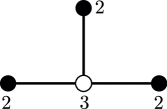
(b) $D_{5,2}$

(c) $D_{7,4}$

Figure 2: The generalized geometries considered in the text. Nodes denote two-cycles, a line connecting two nodes indicates that the cycles intersect each other transversely, and a number next to the node denotes (minus) its self-intersection.

Consider for instance the case in which the small resolution of $X_{\Gamma}$ has two curves $a_{1}$ and $a_{2}$, of self-intersection $-3$ and $-2$ respectively. The two curves intersect at a point. The resulting intersection diagram is shown in figure 2(a). This geometry is one of the “generalized $A$-type” configurations studied in Heckman:2013pva ; DelZotto:2015isa , to which we refer the reader interested in further details. The point of greatest interest to us is that $X_{\Gamma}$ can be understood as a desingularization of $\mathbb{C}^{2}/\Gamma$, with $\Gamma$ a $\mathbb{Z}_{5}$ subgroup of $U(2)$ acting as

$$(z_{1},z_{2})\to(\omega z_{1},\omega^{2}z_{2})\,,$$ (59)

with $\omega=\exp(2\pi i/5)$. The intersection matrix for this geometry, in the $a_{i}$ basis, is

$$q=\begin{pmatrix}-3&1\\ 1&-2\end{pmatrix}\,,$$ (60)

leading to the relations

$$3a_{1}^{*}=a_{2}^{*}\,,\qquad 2a_{2}^{*}=a_{1}^{*}\,.$$ (61)

From here we learn that $H_{1}(S^{3}/\Gamma)=\mathbb{Z}_{5}$, as expected. Given that $2^{-1}=3$ in $\mathbb{Z}_{5}$ we can take either $a_{1}^{*}$ or $a_{2}^{*}$ as generators, let us take $a_{1}^{*}$ for convenience. We have

$$\mathsf{L}_{\Gamma}(\partial a_{1}^{*},\partial a_{1}^{*})\equiv q^{-1}(a_{1}^{*},a_{1}^{*})\equiv\frac{3}{5}\pmod{1}\,.$$ (62)

Note that 3 is not a quadratic residue in $\mathbb{Z}_{5}$, so this linking form is inequivalent to the one with value $\frac{1}{5}$ for the linking number of the generator with itself.

As another illustration, consider the $d=6$, $\mathcal{N}=(1,0)$ compactifications classified in Heckman:2013pva ; Heckman:2015bfa ; Bhardwaj:2015xxa . The associated defect group was discussed in DelZotto:2015isa , where it was shown that for the “generalized $D$-type” singularities, obtained by taking the quotient $\mathbb{C}^{2}/D_{p+q,q}$, one has

$$H_{1}(S^{3}/D_{p+q,q})=\frac{\operatorname{Hom}(H_{2}(X_{D_{p+q,q}}),\mathbb{Z})}{Q(H_{2}(X_{D_{p+q,q}}))}=\mathbb{Z}_{2}\oplus\mathbb{Z}_{2p}\,,$$ (63)

whenever $q$ is even. Consider for example the case $p=3$. In this case $\mathbb{Z}_{2p}\cong\mathbb{Z}_{2}\oplus\mathbb{Z}_{3}$. Up to a sign that we specify below, there is a unique linking form for the $\mathbb{Z}_{3}$ factor, but for the remaining $\mathbb{Z}_{2}\oplus\mathbb{Z}_{2}$ factor we have two possibilities, given by $\mathsf{L}_{\text{even}}$ and $\mathsf{L}_{\text{odd}}$ in (55). And indeed both possibilities appear: a straightforward application of the techniques above shows that the $(p,q)=(3,2)$ case (in figure 2(b)) has intersection form $\mathsf{L}_{\text{even}}$, while the $(p,q)=(3,4)$ case (in figure 2(c)) has a linking form given by $\mathsf{L}_{\text{odd}}$.

Finally, let us consider the “generalized $D_{N}$” theory of type $D_{p+q,q}$ with $(p,q)=(2,7)$. It was shown in DelZotto:2015isa that the defect group in this case is $\mathbb{Z}_{8}$. A computation along the lines described above shows that the linking form is

$$\mathsf{L}_{\Gamma}(\ell,\ell)=\frac{5}{8}\mod 1$$ (64)

with $\ell$ the generator of $H_{1}(S^{3}/D_{9,7})$. Note that 5 is not a residue modulo 8, so this linking form is inequivalent to the naive pairing $\mathsf{L}(\ell,\ell)=\frac{1}{8}$ mod 1. Another inequivalent pairing

$$\mathsf{L}_{\Gamma}(\ell,\ell)=\frac{3}{8}\mod 1$$ (65)

is also realized, for instance by choosing $(p,q)=(2,9)$. More generally, one finds that $S^{3}/D_{p+q,q}$ for $(p,q)=(2,2k+1)$ has pairing

$$\mathsf{L}_{\Gamma}(\ell,\ell)=\frac{3q}{8}\mod 1$$ (66)

despite the defect group always being $\mathbb{Z}_{8}$, so all possible pairings are realized.

Other generalized $D_{N}$ theories can be analyzed similarly, we will briefly state the results without proof. For instance, consider the family of theories $D_{p+q,q}$ with $(p,q)=(3,3k+1)$. One finds that the defect group is $\mathbb{Z}_{3}\oplus\mathbb{Z}_{2}\oplus\mathbb{Z}_{2}$ for $q$ even (or equivalently, $k$ odd), and $\mathbb{Z}_{12}$ for $q$ odd DelZotto:2015isa . In this last case we find the linking form

$$\mathsf{L}_{\Gamma}(\ell,\ell)=-\frac{q}{12}+\frac{1}{2}\mod 1$$ (67)

with $\ell$ the generator of $\mathbb{Z}_{12}$. For $q$ even, we find instead

$$\mathsf{L}_{\Gamma}(\ell_{3},\ell_{3})=\frac{2}{3}\mod 1$$ (68)

with $\ell_{3}$ a generator of the $\mathbb{Z}_{3}$ factor, and

$$\mathsf{L}_{\Gamma}|_{\mathbb{Z}_{2}\oplus\mathbb{Z}_{2}}=\begin{cases}\mathsf{L}_{\text{odd}}&\text{when }q\in 4\mathbb{Z}\\ \mathsf{L}_{\text{even}}&\text{when }q\in 4\mathbb{Z}+2\end{cases}$$ (69)

for the restriction of the linking form to the $\mathbb{Z}_{2}\oplus\mathbb{Z}_{2}$ factor. One can also see that the $(p,q)=(3,3k-1)$ case leads to precisely the same results as the ones we have just given.

3 Comparison with known results in four and six dimensions

Let us summarize the story so far. Quantizing type IIB string theory on a non-compact manifold $\mathcal{M}_{6}\times\mathbb{C}^{2}/\Gamma$ requires a choice of flux boundary conditions on $\mathcal{N}_{9}=\mathcal{M}_{6}\times S^{3}/\Gamma$. Because electric and magnetic flux operators do not commute, there is no canonical “zero flux” boundary condition that we can choose. Instead, the possible boundary conditions for the RR fluxes are states in a Hilbert space acted on by the flux operators $\Phi_{x}$, $x\in\operatorname{Tor}K^{1}(\mathcal{N}_{9})$, with commutation relations

$$\Phi_{x}\Phi_{y}=s(x,y)\Phi_{y}\Phi_{x}\,,$$ (70)

where $s(x,y)$ is a perfect pairing. Maximal commuting subsets of the flux operators are in direct correspondence with maximal isotropic subspaces $L\subset\operatorname{Tor}K^{1}(\mathcal{N}_{9})$ with respect to the perfect pairing $s(x,y)$. Given maximal isotropic $L$, there is a basis of eigenstates $|f;L\rangle$ labeled by cosets $f\in F_{L}=\operatorname{Tor}K^{1}(\mathcal{N}_{9})/L$ with

$$\forall x\in L,\qquad\Phi_{x}|f;L\rangle=s(x,f)|f;L\rangle\,.$$ (71)

These states have boundary flux in a definite coset $f\in F_{L}$, the strongest condition that we can consistently impose. In particular, $f\cong 0$ (restricting the flux to lie along $L$) is the closest we can come to a “zero flux” boundary condition. The resulting quantization depends on the choice of maximal isotropic subspace $L\subset\operatorname{Tor}K^{1}(\mathcal{N}_{9})$.

Note that the flux operators $\Phi_{x}$ generate a Heisenberg group, summarized by the short exact sequence,

$$0\to U(1)\to\mathcal{W}\xrightarrow{\pi}\operatorname{Tor}K^{1}(\mathcal{N}_{9})\to 0\,,$$ (72)

where $\pi(\Phi_{x})=x$. The Hilbert space of flux boundary conditions discussed above is the unique irreducible representation of $\mathcal{W}$, and so the Heisenberg group $\mathcal{W}$ is a convenient avatar for the choice of boundary conditions.

For $\mathcal{N}_{9}=\mathcal{M}_{6}\times S^{3}/\Gamma$ with $\mathcal{M}_{6}$ torsion-free, $K^{1}(\mathcal{N}_{9})$ is the sum of cohomology groups of odd degree and the perfect pairing is

$$s(a_{1}\otimes\ell_{1},a_{2}\otimes\ell_{2})=\exp\biggl{(}2\pi i\,\mathsf{L}_{\Gamma}(\ell_{1},\ell_{2})\,\int_{\mathcal{M}_{6}}a_{1}\smile a_{2}\biggr{)}\,,$$ (73)

where $a_{i}\in H^{1,3,5}(\mathcal{M}_{6})$, $\ell_{i}\in H^{2}(S^{3}/\Gamma)=\Gamma^{\text{ab}}$, and $\mathsf{L}_{\Gamma}$ is the linking pairing for $S^{3}/\Gamma$, which can be computed using the methods described in the previous section. For instance, for $\Gamma\subset SU(2)$ — leading to the $(2,0)$ theories — we find (see also Hikami:2009ze )

$$\begin{array}[]{cccc}\Gamma&G_{\Gamma}&\Gamma^{\text{ab}}&\mathsf{L}_{\Gamma}\\ \hline\cr\mathbb{Z}_{N}&SU(N)&\mathbb{Z}_{N}&\frac{1}{N}\\ \mathrm{Dic}_{(4N-2)}&\mathrm{Spin}(8N)&\mathbb{Z}_{2}\oplus\mathbb{Z}_{2}&\mathsf{L}_{\text{even}}\\ \mathrm{Dic}_{(4N-1)}&\mathrm{Spin}(8N+2)&\mathbb{Z}_{4}&\frac{3}{4}\\ \mathrm{Dic}_{(4N)}&\mathrm{Spin}(8N+4)&\mathbb{Z}_{2}\oplus\mathbb{Z}_{2}&\mathsf{L}_{\text{odd}}\\ \mathrm{Dic}_{(4N+1)}&\mathrm{Spin}(8N+6)&\mathbb{Z}_{4}&\frac{1}{4}\\ 2T&E_{6}&\mathbb{Z}_{3}&\frac{2}{3}\\ 2O&E_{7}&\mathbb{Z}_{2}&\frac{1}{2}\\ 2I&E_{8}&0&0\end{array}$$ (74)

When the defect group $\Gamma^{\text{ab}}$ is cyclic, we list $\mathsf{L}_{\Gamma}(a,a)$ for the generator $a$, whereas for $\Gamma^{\text{ab}}=\mathbb{Z}_{2}\oplus\mathbb{Z}_{2}$, we refer to the two cases in (55).

We emphasize that the correct linking pairing is in general not determined by the defect group. For instance, the defect groups for $\mathrm{Spin}(8N)$ and $\mathrm{Spin}(8N+4)$ are both $\mathbb{Z}_{2}\oplus\mathbb{Z}_{2}$, but the linking pairings are distinct. This has physical consequences, e.g., for S-duality in 4d compactifications of these theories, and we will see that the linking pairings in (74) correctly reproduce known results from the literature. This is a sensitive test of our methods.

3.1 $(2,0)$ theories

This solves the problem of specifying the RR flux boundary conditions for type IIB string theory compactified on $\mathcal{M}_{6}\times\mathbb{C}^{2}/\Gamma$. We now compare our results with known results about the global structure of 6d $(2,0)$ theories with simple Lie algebras. To do so, we use the universal coefficient theorem, which is the short exact sequence (see theorem 2.33 in DavisKirk )

$$0\to H^{n}(X)\otimes A\to H^{n}(X;A)\to\operatorname{Tor}(H^{n+1}(X),A)\to 0\,.$$ (75)

Applying (22) along with the assumption that $\mathcal{M}_{6}$ is torsion-free, we find

$$\operatorname{Tor}K^{1}(\mathcal{M}_{6}\times S^{3}/\Gamma)=H^{1}(\mathcal{M}_{6};\Gamma^{\text{ab}})\oplus H^{3}(\mathcal{M}_{6};\Gamma^{\text{ab}})\oplus H^{5}(\mathcal{M}_{6};\Gamma^{\text{ab}})\,.$$ (76)

Thus, the Heisenberg group can be presented as

$$0\to U(1)\to\mathcal{W}\to H^{1}(\mathcal{M}_{6};\Gamma^{\text{ab}})\oplus H^{3}(\mathcal{M}_{6};\Gamma^{\text{ab}})\oplus H^{5}(\mathcal{M}_{6};\Gamma^{\text{ab}})\to 0\,,$$ (77)

as is typically done in the $(2,0)$ literature. Note, however, that the cohomology theory of $\mathcal{M}_{6}$ with coefficients in $\Gamma^{\text{ab}}$ does not in itself define the perfect pairing $s(x,y)$. Instead, this depends on the topology of $S^{3}/\Gamma$, as we have seen.

Since (73) involves the cup product on $\mathcal{M}_{6}$, the Heisenberg group splits naturally into a direct sum $\mathcal{W}=\mathcal{W}_{1,5}\oplus\mathcal{W}_{3}$, where

$$0\to U(1) \to\mathcal{W}_{1,5}\to H^{1}(\mathcal{M}_{6};\Gamma^{\text{ab}})\oplus H^{5}(\mathcal{M}_{6};\Gamma^{\text{ab}})\to 0\,,$$ (78)

$$0\to U(1) \to\mathcal{W}_{3}\to H^{3}(\mathcal{M}_{6};\Gamma^{\text{ab}})\to 0\,.$$ (79)

The $\mathcal{W}_{1,5}$ factor is associated with D1 and D5 branes wrapping torsional cycles in $S^{3}/\Gamma$, and stretching from infinity to the singularity, giving rise to point and codimension two operators in the six dimensional theory. We also expect to have operators related to these by $SL(2,\mathbb{Z})$ transformations of the IIB background, that is $(p,q)$ 5-branes and $(p,q)$ 1-branes. It would be interesting to understand these operators more fully from the field theoretic viewpoint, but we will not do so here, simply noting that a choice of maximal isotropic subspace within $H^{1}(\mathcal{M}_{6};\Gamma^{\text{ab}})\oplus H^{5}(\mathcal{M}_{6};\Gamma^{\text{ab}})$ can be done canonically, without reference to the details of $\mathcal{M}_{6}$. For example, we can choose $L=H^{1}(\mathcal{M}_{6};\Gamma^{\text{ab}})$, or with equal validity $L=H^{5}(\mathcal{M}_{6};\Gamma^{\text{ab}})$.

Likewise, $\mathcal{W}_{3}$ is associated with D3 branes wrapping torsion cycles in $S^{3}/\Gamma$, giving rise to 2-surface operators in the six dimensional theory. However, unlike before, there is no $\mathcal{M}_{6}$-independent choice of boundary conditions (except in some special cases, see (81) below). This differs from the situation at the classical level, where all background fluxes can be set to zero if desired. Due to the non-commutativity of fluxes in the presence of torsion, this canonical choice ceases to exist in the quantum theory: trying to set all fluxes to zero would be akin to trying to fix both the position and momentum of a particle in ordinary quantum mechanics.

These IIB results have clear implications for 6d $(2,0)$ theories. In order to fully specify the partition function of a six-dimensional $(2,0)$ theory on a manifold $\mathcal{M}_{6}$ we need to specify the background fields for the global 2-form symmetries of the theory. These background fields are inherited from the asymptotic boundary conditions for the $F_{5}$ flux — or somewhat more precisely, from the holonomies of $C_{4}$ on torsion cycles, see Freed:2006ya ; Freed:2006yc and the remarks at the beginning of §2.1. But we have just argued that completely fluxless boundary conditions for $F_{5}$ are impossible. Thus, the background fields for the 2-form symmetries of the $(2,0)$ theory cannot all be set to zero. Instead, only a subset can be fixed, the remainder being summed over. The choice of this subset is a choice of maximal abelian subgroup of the Heisenberg group $\mathcal{W}_{3}$ in (79), equivalently the choice of a maximal isotropic subspace of $H^{3}(\mathcal{M}_{6};\Gamma^{\text{ab}})$.

Indeed, precisely the same structure has been previously argued — by different means — to describe the global structure of $(2,0)$ Witten:1998wy ; Witten:2009at and $(1,0)$ DelZotto:2015isa theories. The IIB viewpoint that we have developed here encompasses all previously understood cases, and allows us to determine the precise commutation relations for the 2-form flux operators, as illustrated above for $\mathbb{C}^{2}/D_{2n}$ and $\mathbb{C}^{2}/D_{p+q,p}$. For instance, the distinction between $\mathsf{L}_{\text{even}}$ and $\mathsf{L}_{\text{odd}}$ for the case $p=3$ with $q$ even should lead to distinct S-duality patterns after compactification on $T^{2}$; to our knowledge this is not yet explored in the literature.

3.2 Theories and metatheories

As we have seen, the $(2,0)$ theories are generally “metatheories”: they have a partition vector — associated to a choice of maximal isotropic subspace $L\subset\Gamma^{\text{ab}}\otimes H^{3}(\mathcal{M}_{6})$ — rather than a partition function. If we can devise a prescription for choosing $L$, independent of the details of $\mathcal{M}_{6}$, then the partition vector becomes a partition function, and we obtain a “genuine” theory. In particular, this is true when

$$L=L_{0}\otimes H^{3}(\mathcal{M}_{6})\,,$$ (80)

where $L_{0}\subset H^{2}(S^{3}/\Gamma)=\Gamma^{\text{ab}}$ is “self-dual,” i.e., equal to its orthogonal complement $L_{0}=L_{0}^{\perp}$ with respect to the linking pairing $\mathsf{L}_{\Gamma}$.

Crucially, since the linking pairing $\mathsf{L}_{\Gamma}$ on $H^{2}(S^{3}/\Gamma)$ is symmetric (unlike the linking pairing $\mathsf{L}$ on $H^{5}(\mathcal{N}_{9})$, which is antisymmetric), self-dual $L_{0}$ need not exist. In particular, one can show that $|L||L^{\perp}|=|\Gamma^{\text{ab}}|$, and so the order of the defect group must be a perfect square. Examining (74), the possibilities corresponding to simple Lie algebras are easily classified:

$$\begin{array}[]{cccc}\mathfrak{g}&\Gamma^{\text{ab}}&L_{0}&G\\ \hline\cr A_{k^{2}-1}&\mathbb{Z}_{k^{2}}&k&SU(k^{2})/\mathbb{Z}_{k}\\ D_{k}&\mathbb{Z}_{2}\oplus\mathbb{Z}_{2}\text{\ or\ }\mathbb{Z}_{4}&(1,1)\text{\ or\ }2&SO(2k)\\ D_{4k}&\mathbb{Z}_{2}\oplus\mathbb{Z}_{2}&(1,0)&Ss(8k)\\ D_{4k}&\mathbb{Z}_{2}\oplus\mathbb{Z}_{2}&(0,1)&Sc(8k)\\ E_{8}&0&0&E_{8}\end{array}$$ (81)

where in each case $L_{0}$ is cyclic and we indicate its generator. Fixing these maximal isotropic subspaces, we obtain genuine $(2,0)$ theories (see, e.g., Tachikawa:2013hya ; Gaiotto:2014kfa ), where $G$ is the 5d gauge group that results from compactification on $S^{1}$ (see below) and $Ss(4k)=\mathrm{Spin}(4k)/\mathbb{Z}_{2}^{(L)}$ and $Sc(4k)=\mathrm{Spin}(4k)/\mathbb{Z}_{2}^{(R)}$ are the semispin groups. Notice in particular that the linking pairing $\mathsf{L}_{\text{even}}$ leads to additional genuine $(2,0)$ theories that are not present for $\mathsf{L}_{\text{odd}}$.

The distinction between metatheories and genuine theories is further illuminated by considering the behavior of extended operators. For instance, the $(2,0)$ theory with Lie algebra $D_{4k}$ contains three types of 2-surface operators, corresponding to the three non-zero elements of the defect group $\mathbb{Z}_{2}\oplus\mathbb{Z}_{2}$. These 2-surface operators are not “mutually local”, in that correlation functions containing multiple types of 2-surface operators will have branch cuts when one type circles another. We can solve this problem by declaring only one type of 2-surface operator to be “genuine” Witten:1998wy ; Kapustin:2014gua ; Gaiotto:2014kfa . The remaining “non-genuine” 2-surface operators are then interpreted as lying at the boundaries of 3-surface operators (the branch cuts), with the correlation functions only topologically dependent on the position of the 3-surfaces.

Indeed, depending on which 2-surface operator we designate as genuine, we obtain one of the genuine theories $SO(8k)$, $Ss(8k)$, or $Sc(8k)$ listed in the table above, where the generator of the maximal isotropic subspace $L_{0}$ corresponds to the genuine 2-surface operator. The other genuine theories also correspond to choosing genuine 2-surface operators in the same manner, but with the added complication that some 2-surface operators fail to be “self-local”, in that two operators of the same type can generate a branch cut upon circling each other.

To see how these properties follow from the string theory picture discussed previously, it is convenient to consider first the conceptually simpler 6d $(1,1)$ theories.

3.3 Wilson and ’t Hooft operators

To obtain 6d $\mathcal{N}=(1,1)$ Yang-Mills theories with simple ADE Lie algebra $\mathfrak{g}_{\Gamma}$, we replace type IIB string theory with type IIA string theory in our discussion above, with $\Gamma\subset SU(2)$. To define the partition function for this theory on a manifold $\mathcal{M}_{6}$ we again need to choose boundary conditions at infinity. The main difference with the IIB case is that in IIA the RR fluxes live in $K^{0}(X)$, instead of $K^{1}(X)$ Moore:1999gb . Repeating the analysis above, mutatis mutandis, we obtain

$$\operatorname{Tor}(K^{0}(\mathcal{M}_{6}\times S^{3}/\Gamma))=(H^{0}(\mathcal{M}_{6})\oplus H^{2}(\mathcal{M}_{6})\oplus H^{4}(\mathcal{M}_{6})\oplus H^{6}(\mathcal{M}_{6}))\otimes\Gamma^{\text{ab}}\,,$$ (82)

so that once more the Heisenberg group splits naturally into two components

$$0\to U(1) \to\mathcal{W}_{0,6}\to H^{0}(\mathcal{M}_{6};\Gamma^{\text{ab}})\oplus H^{6}(\mathcal{M}_{6};\Gamma^{\text{ab}})\to 0\,,$$ (83)

$$0\to U(1) \to\mathcal{W}_{2,4}\to H^{2}(\mathcal{M}_{6};\Gamma^{\text{ab}})\oplus H^{4}(\mathcal{M}_{6};\Gamma^{\text{ab}})\to 0\,,$$ (84)

both with the commutation relations coming from the torsion pairing in $S^{3}/\Gamma$ times the intersection number in $\mathcal{M}_{6}$. As we will see, the Heisenberg algebra $\mathcal{W}_{2,4}$ is associated to Wilson and ’t Hooft operators, and correspondingly the maximal isotropic subspaces of $H^{2}(\mathcal{M}_{6};\Gamma^{\text{ab}})\oplus H^{4}(\mathcal{M}_{6};\Gamma^{\text{ab}})$ are related to the global form of the gauge group. The significance of $\mathcal{W}_{0,6}$ is less clear, and we defer further consideration of it to a future work.

Wrapping a D2 brane on a torsion one-cycle $\sigma_{a}$ of $S^{3}/\Gamma$ and extending it from the singularity off to infinity, we obtain a Wilson line operator in the 6d gauge theory. To determine whether the Wilson line operator is genuine, we move it around a closed path in $\mathcal{M}_{6}$, tracing out a two-cycle $\Sigma_{2}$, and ask whether the correlation function has changed once it returns to its original position. If we initially deform the D2 brane only within a distance $r<r_{0}$ of the singularity, then the net result of the deformation is to add a D2 brane wrapped on $\sigma_{a}\times\Sigma_{2}$ at radius $r=r_{0}$. Extending the deformation outward ($r_{0}\to\infty$) corresponds to moving the wrapped D2 brane far away from the singularity. The Chern-Simons coupling $\oint_{\sigma_{a}\times\Sigma_{2}}C_{3}$ of the wrapped D2 brane contributes a phase to the path integral unless the holonomy of $C_{3}$ on $\sigma_{a}\times\Sigma_{2}$ vanishes. Explicitly, pulling back to $S^{3}/\Gamma\times\Sigma_{2}$, the phase is $\exp(2\pi i\mathsf{L}_{\Gamma}(\mathrm{PD}[\sigma_{a}],f))$ where $\mathrm{PD}$ denotes the Poincaré dual within $S^{3}/\Gamma$ and $f\in\operatorname{Tor}H^{4}(S^{3}/\Gamma\times\Sigma_{2})\cong H^{2}(S^{3}/\Gamma)\otimes H^{2}(\Sigma_{2})\cong H^{2}(S^{3}/\Gamma)$ is the torsion component of the $F_{4}$ flux along $S^{3}/\Gamma\times\Sigma_{2}$. Thus, the correlation function has a branch cut unless the linking pairing $L_{\Gamma}(\mathrm{PD}[\sigma_{a}],f)$ vanishes.

Likewise, a D4 brane wrapped on $\sigma_{b}$ and extended from the singularity to infinity yields a ’t Hooft 3-surface operator in the gauge theory. Consider the link $\Sigma_{2}$ of the 3-surface wrapped by the ’t Hooft operator within $\mathcal{M}_{6}$. The presence of the D4 brane generates torsional flux $f=\mathrm{PD}[\sigma_{b}]$ within $\operatorname{Tor}H^{4}(S^{3}/\Gamma\times\Sigma_{2})\cong H^{2}(S^{3}/\Gamma)$, and so deforming a Wilson line associated to the torsion cycle $\sigma_{a}$ along $\Sigma_{2}$ we pick up a phase $\exp(2\pi i\mathsf{L}_{\Gamma}(\sigma_{a},\sigma_{b}))$: the Wilson and ’t Hooft operators are not mutually local.

Suppose that we wish to designate all Wilson lines as genuine. Per the above discussion, this requires a boundary condition where the torsion component of $[F_{4}]$, classified by $\operatorname{Tor}H^{4}(S^{3}/\Gamma\times\mathcal{M}_{6})\cong\Gamma^{\text{ab}}\otimes H^{2}(\mathcal{M}_{6})$, vanishes. The corresponding maximal isotropic subspace is $L=\Gamma^{\text{ab}}\otimes H^{4}(\mathcal{M}_{6})$. As this choice is independent of the details of $\mathcal{M}_{6}$, it produces a genuine $(1,1)$ theory with Wilson lines classified by $\Gamma^{\text{ab}}=Z(G_{\Gamma})$. In a gauge theory with gauge group $G$, we expect a Wilson line operator for each element of $Z(G)$ (see, e.g., Aharony:2013hda ), so we interpret this theory as the 6d $(1,1)$ theory with simply connected gauge group $G_{\Gamma}$.

More generally, for any subgroup $L_{W}\subseteq\Gamma^{\text{ab}}$, we can choose the maximal isotropic subspace

$$L=[L_{W}\otimes H^{4}(\mathcal{M}_{6})]\oplus[L_{H}\otimes H^{2}(\mathcal{M}_{6})]\,,\qquad L_{H}=L_{W}^{\perp}\,,$$ (85)

for which the Wilson lines $L_{W}$ and ’t Hooft lines $L_{H}=L_{W}^{\perp}$ are genuine. By the same reasoning as above, this is a genuine $(1,1)$ theory with gauge group $G_{\Gamma}/L_{H}$. In this way, the $\mathcal{M}_{6}$-independent maximal isotropic subspaces reproduce the different global forms of the gauge group.

This result can also be understood from the viewpoint of generalized global symmetries Gaiotto:2014kfa . Consider, as an example, the six-dimensional $(1,1)$ theory with algebra $\mathfrak{su}(N)$. The choice of a global form of the gauge group can be understood as a choice of which higher-form symmetries are present in the theory. For instance, if we choose global form $SU(N)$ then there is a $\mathbb{Z}_{N}$ discrete 1-form symmetry counting Wilson lines (which are “genuine”, in this theory), while if we choose global form $SU(N)/\mathbb{Z}_{N}$ there is instead a $\mathbb{Z}_{N}$ 3-form symmetry counting ’t Hooft 3-surface operators. In the former case, we can couple the theory to a background 2-form $\mathbb{Z}_{N}$ gauge field, with the non-trivial gauge bundles classified by $H^{2}(\mathcal{M}_{6};\mathbb{Z}_{N})$. These gauge bundles for the background 2-form should correspond to the background flux $f\in F_{L}$, where $F_{L}$ is given by (11). Thus, the global form $SU(N)$ corresponds to the maximal isotropic subspace $L=H^{4}(\mathcal{M}_{6};\mathbb{Z}_{N})$ (for which $F_{L}\cong H^{2}(\mathcal{M}_{6};\mathbb{Z}_{N})$), in agreement with the above analysis. The case $SU(N)/\mathbb{Z}_{N}$ is analyzed similarly.

3.4 $\mathcal{N}=4$ theories of ADE type

The above discussion is readily generalized to the $(2,0)$ theories, with corresponding changes in the dimensions of branes/operators and the ranks of fluxes. However, as many $(2,0)$ theories do not admit an $\mathcal{M}_{6}$-independent maximal isotropic subspace, see §3.2, it is particularly interesting in this case to consider Lagrangian subspaces that depend on $\mathcal{M}_{6}$. The discussion of the previous section can be summarized as follows: switching to homology using Poincaré duality, the Lagrangian subspace $L\subset H_{1}(S^{3}/\Gamma)\otimes H_{3}(\mathcal{M}_{6})\cong H_{3}(\mathcal{M}_{6};\Gamma^{\text{ab}})$ is the space of cycles on which the holonomy of $C_{4}$ is asymptotically fixed to zero by the boundary conditions. As such, these are the cycles around which we can deform the 2-surface operators without encountering a branch cut. When $L$ is $\mathcal{M}_{6}$ dependent, this means that some but not all branch cuts are eliminated, and in general no 2-surface operators are genuine when deformed around an arbitrary three-cycle.

Having understood the behavior of 6d $(2,0)$ theories in terms of boundary conditions in type IIB string theory, we can apply the same ideas to compactifications of the $(2,0)$ theory. Our goal in the remainder of this section is to demonstrate that the classification of 4d $\mathcal{N}=4$ theories given by Aharony:2013hda (see also Gaiotto:2010be ) is reproduced in this framework. To do so, we consider $T^{2}\times\mathcal{M}_{4}$ compactifications of the $(2,0)$ theories, following a similar approach to Tachikawa Tachikawa:2013hya but using Heisenberg group commutators computed directly in the type IIB picture discussed above, rather than inferred from four dimensional reasoning Gaiotto:2010be ; Aharony:2013hda . The Lie algebras $D_{4k}$ and $D_{4k+2}$ (not analyzed in Tachikawa:2013hya ) provide a particular sensitive test of our reasoning, as the different linking pairings $\mathsf{L}_{\text{even}}$ and $\mathsf{L}_{\text{odd}}$ for these two cases lead to different patterns of 4d S-duality, in agreement with Aharony:2013hda .

First note that, in the absence of torsion on $\mathcal{M}_{4}$, we have by the Künneth formula

$$H^{3}(\mathcal{M}_{4}\times T^{2})=H^{3}(\mathcal{M}_{4})\oplus[H^{2}(\mathcal{M}_{4})\otimes H^{1}(T^{2})]\oplus H^{1}(\mathcal{M}_{4})\,.$$ (86)

Again for degree reasons we have a natural splitting of the associated Heisenberg group $\mathcal{W}_{3}=\mathcal{W}_{1,3}\oplus\mathcal{W}_{2}$, with

$$0\to U(1) \to\mathcal{W}_{1,3}\to H^{1}(\mathcal{M}_{4};\Gamma^{\text{ab}})\oplus H^{3}(\mathcal{M}_{4};\Gamma^{\text{ab}})\to 0\,,$$ (87)

$$0\to U(1) \to\mathcal{W}_{2}\to H^{2}(\mathcal{M}_{4})\otimes H^{1}(T^{2})\otimes\Gamma^{\text{ab}}\to 0\,.$$ (88)

The Heisenberg group $\mathcal{W}_{1,3}$ is associated to point and 2-surface operators in the 4d theory. Noting that, $\mathcal{M}_{4}$ and $T^{2}$-independent choices of maximal isotropic subspace are always possible within this factor, such as $L_{1,3}=H^{1}(\mathcal{M}_{4};\Gamma^{\text{ab}})$ or $L_{1,3}=H^{3}(\mathcal{M}_{4};\Gamma^{\text{ab}})$, we ignore it for the time being, instead focusing on the factor $\mathcal{W}_{2}$ describing line operators.

To obtain genuine 4d theories, we consider $\mathcal{M}_{4}$-independent maximal isotropic subspaces of $H^{2}(\mathcal{M}_{4})\otimes H^{1}(T^{2})\otimes\Gamma^{\text{ab}}$. These are of the form

$$L=H^{2}(\mathcal{M}_{4})\otimes L_{T^{2}}$$ (89)

where $L_{T^{2}}$ is a maximal isotropic subspace of $H^{1}(T^{2};\Gamma^{\text{ab}})$, corresponding to the Heisenberg algebra

$$0\to U(1)\to\mathcal{W}_{T^{2}}\to H^{1}(T^{2};\Gamma^{\text{ab}})\to 0\,.$$ (90)

Since a maximal isotropic subspace of $H^{1}(T^{2};\Gamma^{\text{ab}})$ always exists there are genuine theories corresponding to every Lie algebra, unlike in six dimensions. Instead, the absence of a genuine six dimensional theory causes a “modular anomaly”: tracing a closed path in the complex structure moduli space of the torus changes the partition function.

In particular, the partition function is generally not a modular-invariant function of the holomorphic gauge coupling $\tau$. From the 6d perspective, $\tau$ is the complex structure of the torus and modular transformations $\tau\to\frac{a\tau+b}{c\tau+d}$ are large diffeomorphisms in the background metric. Thus, the failure of modular invariance (in the absence of additional background fields along the torus) is the result of a 6d anomaly in large diffeomorphisms. Depending on the 6d anomaly, a characteristic pattern of S-dualities is generated, as in, e.g., Aharony:2013hda .

Note that if we view fixed $\tau$ as part of the defining data of the theory then we would not consider the non-invariance of the partition function under $SL(2,\mathbb{Z})$ transformations of $\tau$ to be a 4d anomaly, but rather a consequence of deforming along a fixed line from one theory to another. On the other hand, when considering four-dimensional backgrounds with varying $\tau$, the anomaly viewpoint becomes more natural. We revisit this point below in the context of theories with codimension-two duality defects.

Thus, for each maximal isotropic subspace of $L_{T^{2}}\subset H^{1}(T^{2};\Gamma^{\text{ab}})$ there is a genuine 4d $\mathcal{N}=4$ theory. Wrapping the 2-surface operators of the 6d $(2,0)$ theory on different cycles of the torus, we obtain different types of 4d line operators. For instance, reducing the $(2,0)$ theory first on the $A$ cycle of the torus, we obtain a five-dimensional gauge theory, with Wilson line and ’t Hooft 2-surface operators. Reducing again on the $B$ cycle, the ’t Hooft operators become lines. Thus, 2-surface operators wrapped around the $A$ and $B$ cycles are Wilson and ’t Hooft lines, respectively, whereas those wrapped around a combination of the two are dyonic lines.

We can identify the genuine theory in question by specifying which of these line operators are genuine. In particular, by the same reasoning as in the previous section, there is a one-to-one correspondence between the elements of the maximal isotropic subspace $L_{T^{2}}$ and the genuine line operators in the 4d theory, and so the result can be directly compared with Aharony:2013hda .

Consider for example the $\mathcal{N}=4$ theories with Lie algebra $\mathfrak{su}(N)$, corresponding to the $A_{N-1}$ $(2,0)$ theory on a torus. In general $H^{1}(T^{2};\Gamma^{\text{ab}})=H^{1}(T^{2})\otimes\Gamma^{\text{ab}}=\Gamma^{\text{ab}}\oplus\Gamma^{\text{ab}}$ with the perfect pairing $s(a,b)=\exp(2\pi i\mathsf{L}_{T^{2}}(a,b))$, where $\mathsf{L}_{T^{2}}$ is the linking pairing on $S^{3}/\Gamma\times T^{2}$

$$\mathsf{L}_{T^{2}}(a,b)=\mathsf{L}_{\Gamma}(\pi_{A}(a),\pi_{B}(b))-\mathsf{L}_{\Gamma}(\pi_{B}(a),\pi_{A}(b))\,\qquad a,b\in\Gamma^{\text{ab}}\oplus\Gamma^{\text{ab}}\,,$$ (91)

and $\pi_{A}:\Gamma^{\text{ab}}\oplus\Gamma^{\text{ab}}\to\Gamma^{\text{ab}}$ and $\pi_{B}:\Gamma^{\text{ab}}\oplus\Gamma^{\text{ab}}\to\Gamma^{\text{ab}}$ project onto the first and second summand, respectively. In the $\mathfrak{su}(N)$ case, $\Gamma^{\text{ab}}=\Gamma=\mathbb{Z}_{N}$, and we obtain the perfect pairing

$$s(e_{1}\mathbf{p}+m_{1}\mathbf{q},e_{2}\mathbf{p}+m_{2}\mathbf{q})=\exp\biggl{(}\frac{2\pi i}{N}(e_{1}m_{2}-e_{2}m_{1})\biggr{)}$$ (92)

from (74), where $\mathbf{p}$ and $\mathbf{q}$ denote the $A$ and $B$ cycles of the torus, respectively. Here $e_{i}$ and $m_{i}$ denote the Wilson and ’t Hooft charges of the associated line operators, respectively. For instance, $L=\{m\mathbf{q}|0\leq m<N\}$ is a maximal isotropic subspace whose elements correspond to ’t Hooft lines of every possible $\mathbb{Z}_{N}$ charge; the associated gauge theory is therefore $(SU(N)/\mathbb{Z}_{N})_{0}$ in the notation of Aharony:2013hda .

For any fixed $N$, it is a simple exercise to enumerate the maximal isotropic subspaces of $\mathbb{Z}_{N}\oplus\mathbb{Z}_{N}$ with respect to the perfect pairing (92). For instance, the case $N=3$ is shown in figure 3, with results that are easily seen to agree with Aharony:2013hda . More generally, flux operators $\Phi_{1}$ and $\Phi_{2}$ commute if

$$e_{1}m_{2}-e_{2}m_{1}\equiv 0\pmod{N}\,.$$ (93)

This is the same as the mutual locality constraint found in Aharony:2013hda , so the results will agree in general.

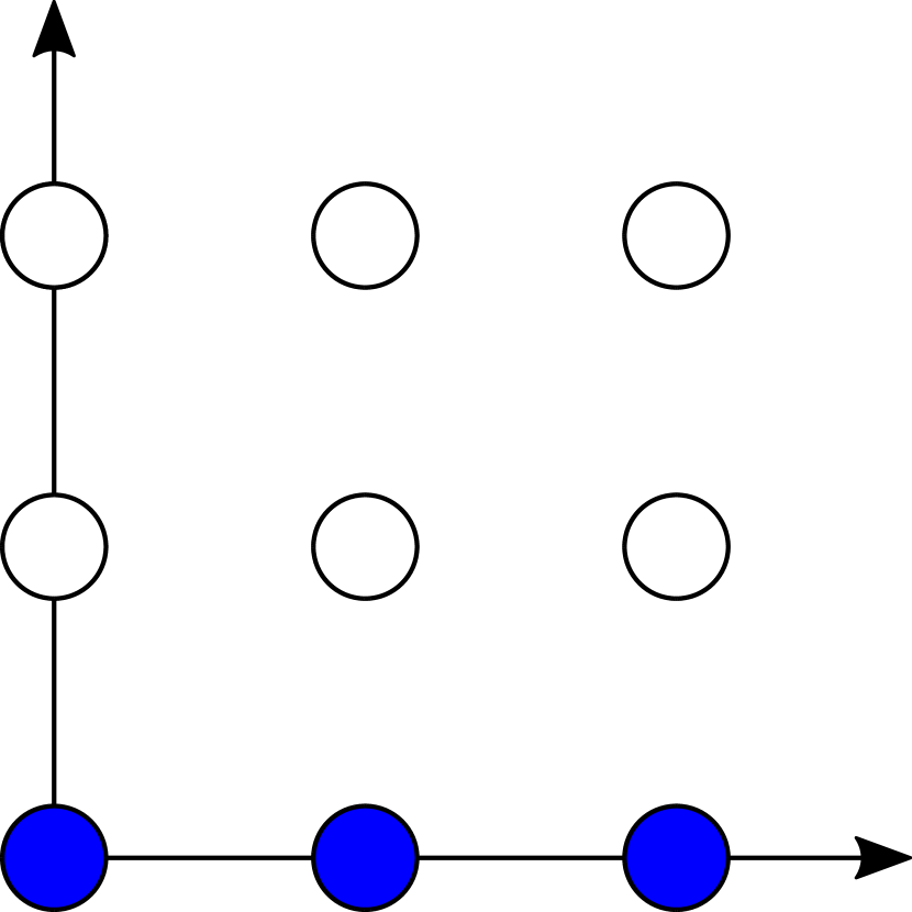
(a) $SU(3)$

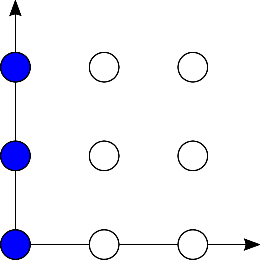
(b) $(SU(3)/\mathbb{Z}_{3})_{0}$

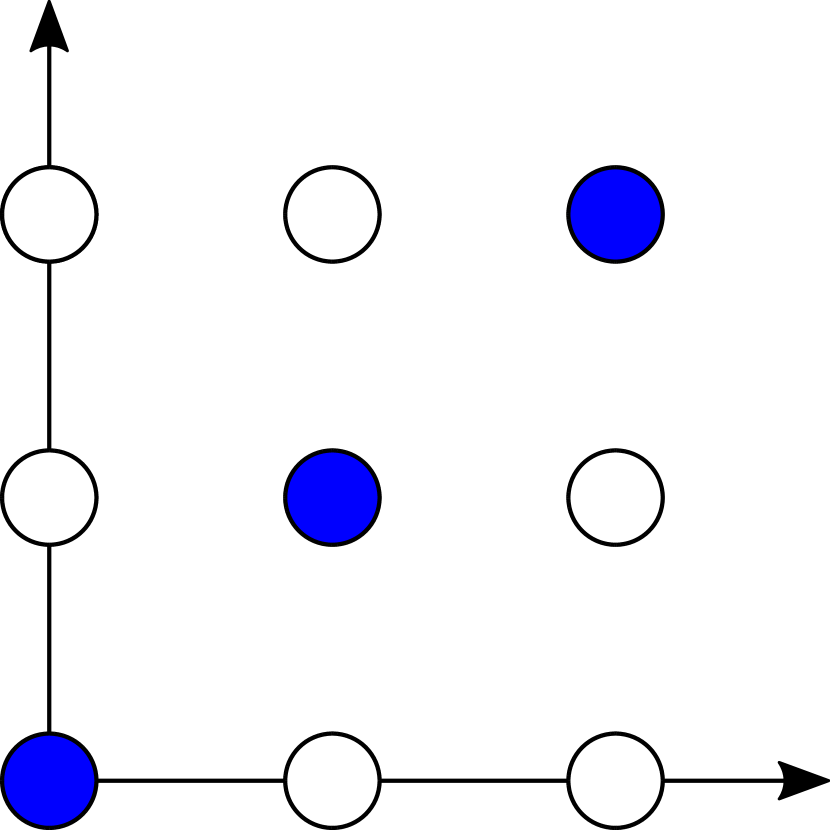
(c) $(SU(3)/\mathbb{Z}_{3})_{1}$

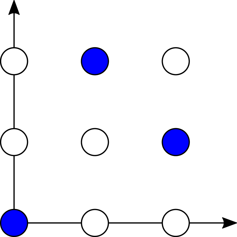
(d) $(SU(3)/\mathbb{Z}_{3})_{2}$

Figure 3: Maximal isotropic subspace of $H^{1}(T^{2};\mathbb{Z}_{3})=\mathbb{Z}_{3}\oplus\mathbb{Z}_{3}$ with respect to the perfect pairing (92). We have labelled the possibilities using the nomenclature of Aharony:2013hda . Each filled dot corresponds to a genuine line operator.

The $\mathfrak{so}(4k+2)$ and $E_{6,7,8}$ theories are handled similarly. However, the case $\mathfrak{so}(4k)$ deserves special attention, as the defect group $\Gamma^{\text{ab}}=\mathbb{Z}_{2}\oplus\mathbb{Z}_{2}$ is not cyclic, and there are multiple possible linking pairings, each with different consequences. For $\mathfrak{so}(8k)$, the linking pairing is $\mathsf{L}_{\Gamma}=\mathsf{L}_{\text{even}}$ per (74), so we obtain the perfect pairing

$$s(e_{1}\mathbf{p}+\tilde{e}_{1}\tilde{\mathbf{p}}+m_{1}\mathbf{q}+\tilde{m}_{1}\tilde{\mathbf{q}},e_{2}\mathbf{p}+\tilde{e}_{2}\tilde{\mathbf{p}}+m_{2}\mathbf{q}+\tilde{m}_{2}\tilde{\mathbf{q}})=(-1)^{e_{1}\tilde{m}_{2}+\tilde{e}_{1}m_{2}+e_{2}\tilde{m}_{1}+\tilde{e}_{2}m_{1}}$$ (94)

using (91), where $\mathbf{p}$ and $\tilde{\mathbf{p}}$ denote the $A$ cycle of the torus tensored with the two generators of $\mathbb{Z}_{2}\oplus\mathbb{Z}_{2}$ and likewise for $\mathbf{q}$ and $\tilde{\mathbf{q}}$. For $\mathfrak{so}(8k+4)$ the linking pairing is $\mathsf{L}_{\Gamma}=\mathsf{L}_{\text{odd}}$, so we obtain instead

$$s(e_{1}\mathbf{p}+\tilde{e}_{1}\tilde{\mathbf{p}}+m_{1}\mathbf{q}+\tilde{m}_{1}\tilde{\mathbf{q}},e_{2}\mathbf{p}+\tilde{e}_{2}\tilde{\mathbf{p}}+m_{2}\mathbf{q}+\tilde{m}_{2}\tilde{\mathbf{q}})=(-1)^{e_{1}m_{2}+\tilde{e}_{1}\tilde{m}_{2}+e_{2}m_{1}+\tilde{e}_{2}\tilde{m}_{1}}\,.$$ (95)

These agree with (5.4) of Aharony:2013hda , which is a sensitive check of our analysis.

The above analysis generalizes readily to compactifications of the $(2,0)$ theory on an arbitrary compact Riemann surface $\Sigma$; $\mathcal{M}_{4}$-independent maximal isotropic subspaces are now of the form $L=H^{2}(\mathcal{M}_{4})\otimes L_{\Sigma}$, associated to the Heisenberg group $0\to U(1)\to\mathcal{W}_{\Sigma}\to H^{1}(\Sigma)\otimes\Gamma^{\text{ab}}$, with the perfect pairing $s(c_{1}\otimes\ell_{1},c_{2}\otimes\ell_{2})=\exp\Bigl{(}2\pi i\,(c_{1}\circ c_{2})\,\mathsf{L}_{\Gamma}(\ell_{1},\ell_{2})\Bigr{)}$, where $\circ$ is the intersection form on $\Sigma$. It would be interesting to understand how adding punctures on $\Sigma$—as in class $\mathcal{S}$ constructions—changes this story.

3.5 Fractional instanton numbers and the linking form

Although this is somewhat outside the main line of development of our paper, we point out that in the $\mathcal{N}=4$ cases one can give a simple expression for the fractional instanton numbers for $G_{\Gamma}/\Gamma^{\text{ab}}$ bundles, as computed in Witten:2000nv (see also Aharony:2013hda ) in terms of the linking pairing discussed above. Let us assume that $\mathcal{M}_{4}$ has no torsion and also that it is a Spin manifold. Consider the class $w_{2}\in H^{2}(\mathcal{M}_{4};\Gamma^{\text{ab}})$ measuring the obstruction to lifting the given $G_{\Gamma}/Z(G_{\Gamma})=G_{\Gamma}/\Gamma^{\text{ab}}$ bundle to $G_{\Gamma}$. Since $\operatorname{Tor}H^{4}(\mathcal{M}_{4}\times S^{3}/\Gamma)\cong H^{2}(\mathcal{M}_{4};\Gamma^{\text{ab}})$ along the same lines as above, we can rewrite this as a class $\widehat{w}_{2}\in\operatorname{Tor}H^{4}(\mathcal{M}_{4}\times S^{3}/\Gamma)$. Denoting by $\hat{\mathsf{L}}$ the linking form in $\mathcal{M}_{4}\times S^{3}/\Gamma$, one can check that the fractional instanton number can be expressed as

$$n_{\text{inst}}\equiv\frac{1}{2}\hat{\mathsf{L}}(\widehat{w}_{2},\widehat{w}_{2})\pmod{1}\,,$$ (96)

in the conventions where the minimal local $G_{\Gamma}$-instanton on $\mathbb{R}^{4}$ has instanton number 1. This relation is less surprising if we recall the fact that the fractional instanton number $n_{\text{inst}}$ encodes the change in the partition function of $\mathcal{N}=4$ super-Yang-Mills under $\tau\to\tau+1$, up to a factor $c(\mathcal{M}_{4})$ that depends on the topology of $\mathcal{M}_{4}$ but not on $w_{2}$ Vafa:1994tf :

$$Z_{w_{2}}(\tau+1)=\exp\biggl{(}2\pi i(c(\mathcal{M}_{4})+n_{\text{inst}})\biggr{)}Z_{w_{2}}(\tau)\,.$$ (97)

From the type IIB string theory perspective this is a change in the phase of the partition function resulting from a large diffeomorphism of the $T^{2}$ factor in the $\mathcal{M}_{4}\times T^{2}\times\mathbb{C}^{2}/\Gamma$ geometry, in the presence of a RR 5-form flux given by $\widehat{w}_{2}\otimes x$, with $x$ a generator of $H^{1}(T^{2})$.

(a) Action of the large diff on IIB.

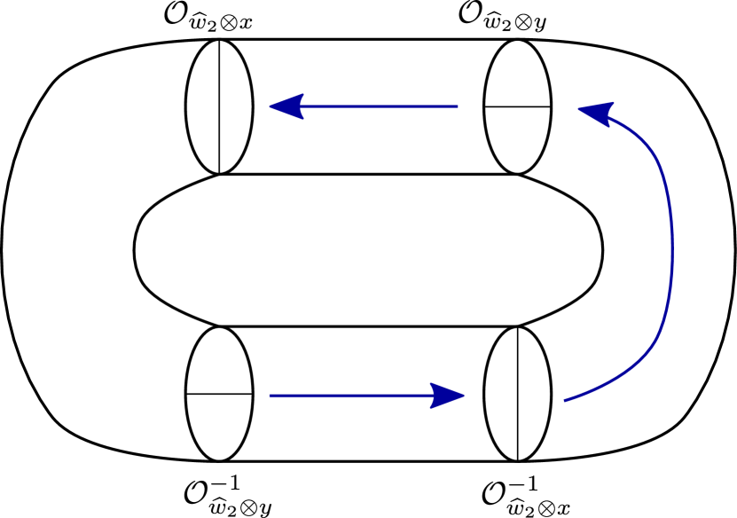
(b) Building the commutator.

Figure 4: 4(a) The fractional instanton number can be viewed as the anomaly coming from a large diffeomorphism in the presence background torsion flux. At the level of the fluxes, this can be implemented by the insertion of suitable operators in the anomaly theory. 4(b) Gluing two copies of the configuration giving the anomaly to two configurations without flux we obtain the anomaly theory with four operator insertions. Bringing the operators together we obtain the commutator, a c-number.

As such, a rough argument for (96) is as follows. Heuristically, we could express the path integral of IIB string theory on a manifold $X_{10}$ with background flux $F$ as the the partition function of the anomaly theory $\mathcal{A}$ on a manifold $Y_{11}$ with $\partial Y_{11}=X_{10}$, and an insertion in $Y_{11}$ of an appropriate flux operator $\Phi_{F}$ (see for instance Witten:1998wy for a similar construction in the context of AdS/CFT). In our situation, depicted in figure 4(a), we are interested in computing the partition function of $\mathcal{A}$ on a cylinder with flux $\widehat{w}_{2}\otimes x$ on one end, and (due to the large diff on the $T^{2}$ factor) a flux $\widehat{w}_{2}\otimes(x+y)$ on the other end. In order to create these fluxes, we introduce operators $\Phi_{\widehat{w}_{2}\otimes x}$ and $\Phi_{\widehat{w}_{2}\otimes y}$ into the bulk of the anomaly theory.

Now take two copies of the cylinder constructed above, and glue them together, along with two trivial cylinders, into a torus, as in figure 4(b). Bringing the four insertions together we obtain the commutator $s(\widehat{w}_{2}\otimes x,\widehat{w}_{2}\otimes y)$ which is a c-number, and can be taken out of the path integral. The $c(\mathcal{M}_{4})$ factor in (97) is associated to the change in the partition function with no flux, so it is natural to conjecture that it is associated with the value of the partition function in the absence of $\Phi_{F}$ insertions. Removing this overall factor, the construction implies that

$$s(\widehat{w}_{2}\otimes x,\widehat{w}_{2}\otimes y)=\biggl{[}\exp(2\pi i\,n_{\text{inst}})\biggr{]}^{2}\,.$$ (98)

Using the relations between $s$ and the linking form given above, this implies (96) up to a sign, which depends on choices of orientation that we have not been careful about.

The above argument is somewhat heuristic. It would be interesting to work it out in detail and determine its implications beyond the $\mathcal{N}=4$ case. It seems natural to conjecture, for instance, that (96) still holds if we consider $(1,0)$ theories compactified on $T^{2}$. Even though the resulting theory may be non-Lagrangian, (96) is a natural guess for the behavior of the partition function in the presence of backgrounds for the 1-form symmetries.

3.6 Product groups

Consider the case of the $E_{8}$ theory in six-dimensions, arising from IIB on $\mathbb{C}^{2}/E_{8}$. Since $H^{2}(S^{3}/E_{8})=0$ the $(2,0)$ theory of $\mathfrak{e}_{8}$ type is a genuine six-dimensional theory: no choice of IIB boundary conditions at infinity is needed in order to define the theory on any six-manifold. This implies, in particular, the well-known fact that the $\mathcal{N}=4$ theory with gauge group $E_{8}$ is invariant under $SL(2,\mathbb{Z})$ dualities. The group $E_{8}$ has a maximal subgroup $(E_{6}\times SU(3))/\mathbb{Z}_{3}$, and one can check that the $\mathcal{N}=4$ theory with this gauge group is also invariant under $SL(2,\mathbb{Z})$.

We can reproduce this result from our geometric perspective, by showing that there is a genuine six-dimensional theory of type $\mathfrak{e}_{6}\oplus\mathfrak{su}(3)$. Consider a local $\mathrm{K3}$ with singularities of type locally $\mathbb{C}^{2}/E_{6}$ and $\mathbb{C}^{2}/\mathbb{Z}_{3}$. We link the singularities by small rational homology spheres $S^{3}/E_{6}$ and $S^{3}/\mathbb{Z}_{3}$, with total manifold their disjoint union $S_{u}\coloneqq S^{3}/E_{6}\sqcup S^{3}/\mathbb{Z}_{3}$. From (74) we obtain

$$H^{2}(S_{u})=H^{2}(S^{3}/E_{6})\oplus H^{2}(S^{3}/\mathbb{Z}_{3})=\mathbb{Z}_{3}\oplus\mathbb{Z}_{3}$$ (99)

with linking form

$$\mathsf{L}_{u}=\mathsf{L}_{E_{6}}\oplus\mathsf{L}_{\mathbb{Z}_{3}}=\begin{pmatrix}\frac{2}{3}&0\\ 0&\frac{1}{3}\end{pmatrix}\,.$$ (100)

Let $a$ and $b$ be the generators of $H^{2}(S_{u})$ corresponding to the $H^{2}(S^{3}/E_{6})$ and $H^{2}(S^{3}/\mathbb{Z}_{3})$ factors, respectively. Because $\mathsf{L}_{u}(a+b,a+b)=0$, $H^{2}(S_{u})$ has a self-dual subspace generated by $a+b$ (as well as one generated by $a-b$). Associated to this, there is a maximal isotropic subspace of $H^{2}(S_{u})\otimes H^{3}(\mathcal{M}_{6})$ given by

$$L_{u}=\operatorname{Span}(a+b)\otimes H^{3}(\mathcal{M}_{6})\,.$$ (101)

Following the same reasoning as above, after reduction on $T^{2}$ we obtain a 4d theory with line operators that carry equal charge under the $\mathbb{Z}_{3}$ 1-form symmetries associated to $\mathfrak{e}_{6}$ and $\mathfrak{su}(3)$, hence the global form of the gauge group is indeed $(E_{6}\times SU(3))/\mathbb{Z}_{3}$.

We emphasize that in this last example it was essential that $\mathsf{L}_{E_{6}}=-\mathsf{L}_{\mathbb{Z}_{3}}$, so this is another sensitive check of our arguments. This condition can also be understood along the lines of the previous section: because of the change in sign of the linking form, the induced fractional instanton numbers associated to the two factors are equal and opposite, so that the $\tau\to\tau+1$ transformation becomes anomaly-free.

Similar checks can be performed for the rest of the maximal subgroups of $E_{8}$. For instance, $(Spin(10)\times SU(4))/\mathbb{Z}_{4}$ is another example where the precise signs in (74) are crucial to get the right results. An interesting case is $(SU(5)\times SU(5))/\mathbb{Z}_{5}$, for which $H^{2}(S^{3}/\mathbb{Z}_{5}\sqcup S^{3}/\mathbb{Z}_{5})=\mathbb{Z}_{5}\oplus\mathbb{Z}_{5}$ with linking pairing

$$\mathsf{L}=\begin{pmatrix}\frac{1}{5}&0\\ 0&\frac{1}{5}\end{pmatrix}\,.$$ (102)

Since $2^{2}\equiv-1$ mod 5 and $\gcd(2,5)=1$, we can perform an invertible change of basis $a^{\prime}=2a$ of the first $\mathbb{Z}_{5}$ factor so that the linking pairing becomes

$$\mathsf{L}=\begin{pmatrix}-\frac{1}{5}&0\\ 0&\frac{1}{5}\end{pmatrix}$$ (103)

and we can proceed as above.

As pointed out in Vafa:1994tf , there are self-dual $\mathcal{N}=4$ theories with gauge group $(SU(N)\times SU(N))/\mathbb{Z}_{N}$ for any $N$. At first, this poses a bit of a puzzle, since in general there is no $n$ such that $n^{2}\equiv-1$ mod $N$. For instance, for $N$ prime, the condition for such an $n$ to exist (i.e., for $-1$ to be a quadratic residue) is that $N\equiv 1$ mod 4. Choose $N=3$, for example. The linking pairing is

$$\mathsf{L}=\begin{pmatrix}\frac{1}{3}&0\\ 0&\frac{1}{3}\end{pmatrix}$$ (104)

and it is easy to see that $H^{2}(S_{u})$ has no self-dual subspaces.

The resolution of the puzzle is that the theories described in Vafa:1994tf are really of the form $(\overline{SU(N)}\times SU(N))/\mathbb{Z}_{N}$, meaning that in the IIB string theory realization the 16 supercharges preserved by the first factor are precisely the 16 supercharges broken by the second factor, as in brane-antibrane systems. In the deep infrared, the two $A_{N-1}$ theories decouple, and each is invariant under 16 supercharges. However, the preserved supercharges have opposite chiralities ($(2,0)$ versus $(0,2)$), and the full theory is non-supersymmetric at the massive level.

Geometrically, this is achieved by gluing ALE spaces with opposite orientation to each other. The change of orientation flips the overall sign of the intersection form on the ALE space, which likewise flips the sign of the linking pairing on $S_{3}/\mathbb{Z}_{N}$ by (50). The correct linking pairing on $H^{2}(S_{u})$ is therefore

$$\mathsf{L}=\begin{pmatrix}-\frac{1}{N}&0\\ 0&\frac{1}{N}\end{pmatrix}$$ (105)

which admits self-dual subspaces, such as $\operatorname{Span}(a+b)$.

4 Self-dual boundary conditions

In the previous sections we have discussed how a careful treatment of boundary conditions in IIB string theory in $\mathcal{M}_{6}\times\mathbb{C}^{2}/\Gamma$ allows us to reproduce the known global structure of $(2,0)$ theories of type $\mathfrak{g}_{\Gamma}$ on $\mathcal{M}_{6}$, giving in particular a systematic way of understanding the set of discrete 2-form symmetries of the $(2,0)$ theory and their commutation relations, as encoded in the Heisenberg group

$$0\to U(1)\to\mathcal{W}_{3}\to H^{3}(\mathcal{M}_{6},\Gamma^{\text{ab}})\to 0\,.$$ (106)

We have seen that $\mathcal{W}_{3}$ can be naturally understood as the group of asymptotic fluxes for the self-dual RR 5-form on $\mathcal{M}_{6}\times\mathbb{C}^{2}/\Gamma$. The known classification of $\mathcal{N}=4$ theories arises beautifully from this viewpoint.

Have understood these rather subtle properties of the 6d $(2,0)$ and 4d $\mathcal{N}=4$ theories from the IIB viewpoint, the following question naturally arises. Say that we choose $\mathcal{M}_{6}=\mathcal{M}_{4}\times\Sigma$, as above. In choosing boundary conditions for type IIB on $\mathcal{M}_{4}\times\Sigma\times\mathbb{C}^{2}/\Gamma$ we generally need to choose between breaking large diffeomorphisms on $\Sigma$ or on $\mathcal{M}_{4}$. What makes the IIB boundary conditions that are invariant under the large diffeomorphisms of $\mathcal{M}_{4}$ special from the IIB viewpoint? The answer, clearly, is that there is nothing special about them from the 10d perspective. As such, it is in principle an interesting question to choose different boundary conditions and examine their consequences. In fact, we will argue that in some contexts it is more natural to choose boundary conditions that are invariant under large diffeomorphisms of $\Sigma$. Perhaps surprisingly, we show that these alternate “self-dual” boundary conditions are possible whenever $\mathcal{M}_{4}$ satisfies a few basic assumptions, regardless of whether a genuine $(2,0)$ theory exists in six dimensions.

4.1 On the global structure of $\mathcal{N}=4$ theories with duality defects

As a warm-up, and to provide additional motivation, we first describe a situation where it becomes impossible to choose boundary conditions that are invariant under large diffeomorphisms of $\mathcal{M}_{4}$.

We consider the $(2,0)$ theory of type $\mathfrak{g}_{\Gamma}$ compactified on $\mathcal{M}_{6}=\mathrm{K3}\times\Sigma$, where $\Sigma$ is a Riemann surface and the $\mathrm{K3}$ is elliptically fibered. More concretely, we construct $\mathrm{K3}$ as a hypersurface $\{P=0\}$ of degree $(12,6)$ in a toric space $Y$ described by the gauged linear sigma model with charges

$$\begin{array}[]{c|ccccc}&u_{1}&u_{2}&x&y&z\\ \hline\cr\mathbb{C}^{*}_{1}&1&1&4&6&0\\ \mathbb{C}^{*}&0&0&2&3&1\end{array}$$ (107)

We can write the fibration in Weierstrass form

$$P=-y^{2}+x^{3}+f(u_{1},u_{2})xz^{4}+g(u_{1},u_{2})z^{6}$$ (108)

where $f$ and $g$ are sections of the line bundles $\mathcal{O}_{\mathbb{P}^{1}}(8)$ and $\mathcal{O}_{\mathbb{P}^{1}}(12)$, respectively. (That is, locally they are homogeneous functions of $s_{1},s_{2}$ of degrees 8 and 12, respectively.)

There is a fibration map $\pi\colon\mathrm{K3}\to\mathbb{P}^{1}$ induced by the ambient space fibration $\pi_{a}\colon Y\to\mathbb{P}^{1}$

$$\pi_{a}(u_{1},u_{2},x,y,z)=(u_{1},u_{2})\,.$$ (109)

The generic fiber $\pi^{-1}(u_{1},u_{2})$ is $T^{2}$. The Calabi-Yau space $\mathrm{K3}$ has a section, namely an embedding $\mathbb{P}^{1}\to X$ intersecting each fiber once, given by $\{z=0\}\cap\{P=0\}$.

There are two interesting limits to consider. When the volume of $\Sigma$ is very small, we recover a 4d $\mathcal{N}=4$ theory on $\mathrm{K3}$ along the same lines as we have already discussed. If instead the volume of the $T^{2}$ fiber of $\mathrm{K3}$ is very small, we expect an effective local description in terms of 4d $\mathcal{N}=4$ SYM on $\mathbb{P}^{1}\times\Sigma$ with algebra $\mathfrak{g}_{\Gamma}$. However, this description is qualitatively different from the previous case, due to the presence of duality defects. Recall that the complexified gauge coupling of the $\mathcal{N}=4$ theory is given by the complex structure of the $T^{2}$ fiber. As the fibration is non-trivial in this case, the gauge coupling varies across $\mathcal{M}_{4}=\mathbb{P}^{1}\times\Sigma$, and is now better viewed as a background field, rather than a “constant”. There are codimension two loci along the $\mathbb{P}^{1}\times\Sigma$ base—the duality defects—located at the vanishing points of the discriminant

$$\Delta(u_{1},u_{2})=4f(u_{1},u_{2})^{3}+27g(u_{1},u_{2})^{2}\,,$$ (110)

around which the complexified gauge coupling has $SL(2,\mathbb{Z})$ monodromies. Notice that $\Delta$ is a section of $\mathcal{O}_{\mathbb{P}^{1}}(24)$, so generically it vanishes at 24 points in the base $\mathbb{P}^{1}$.

For a generic fibration, it is easy to see that the monodromy group for loops beginning and ending at any fixed base point is the entire $SL(2,\mathbb{Z})$. As an explicit example, let us start with a class of $\mathrm{K3}$ manifolds introduced by Sen Sen:1996vd , where

$$f(s_{1},s_{2}) =\alpha Q(s_{i})^{2}\,, g(s_{1},s_{2}) =Q(s_{i})^{3}\,, Q(s_{i}) =\prod_{i=1}^{4}(s_{1}-a_{i}s_{2})\,,$$ (111)

with $\alpha$ and $a_{i}$ arbitrary complex constants and $a_{i}\neq a_{j}$ for $i\neq j$. The monodromy around each zero of $Q$ is given by

$$\mathsf{M}=\begin{pmatrix}-1&0\\ 0&-1\end{pmatrix}\,.$$ (112)

These $\mathrm{K3}$ manifolds have the peculiarity that the complex structure of the torus is constant. In fact they have a familiar interpretation in the context of F-theory Vafa:1996xn , where each defect corresponds to four D7 branes on top of an O7^- plane Sen:1996vd . In this configuration we have

$$\Delta=(4\alpha^{3}+27)Q(s_{i})^{6}\,.$$ (113)

That is, there are six zeroes of $\Delta$ coalescing on each zero of $Q(s_{i})$. We now study what happens around each zero of $Q(s_{i})$ when we perturb $f,g$ away from the special form (111). The answer is well known in the context of F-theory (and before that, from the analysis of the Seiberg-Witten solution of $\mathcal{N}=2$ $SU(2)$ with four flavours Seiberg:1994rs ; Seiberg:1994aj ): the six zeroes of $\Delta$ split into four mutually local degenerations (the D7 branes, in F-theory) and two mutually non-local degenerations (the O7^- plane).

To show explicitly that the monodromy group is the full $SL(2,\mathbb{Z})$, we choose an explicit basis for the geometry, following the conventions of Gaberdiel:1998mv ; DeWolfe:1998zf . The defect described above splits into four degenerations of type $\mathsf{A}$, one of type $\mathsf{B}$ and one of type $\mathsf{C}$. The $\mathsf{A}$ degenerations are associated with degenerations the $(1,0)$ cycle of the $T^{2}$, the $\mathsf{B}$ with degenerations of the $(1,-1)$ cycle, and $\mathsf{C}$ with degenerations of the $(1,1)$ cycle (all defined relative to a common canonical basepoint). The $SL(2,\mathbb{Z})$ monodromies associated to these degenerations are

$$\mathsf{M}_{\mathsf{A}}=\begin{pmatrix}1&-1\\ 0&1\end{pmatrix}\quad;\quad\mathsf{M}_{\mathsf{B}}=\begin{pmatrix}0&-1\\ 1&2\end{pmatrix}\quad;\quad\mathsf{M}_{\mathsf{C}}=\begin{pmatrix}2&-1\\ 1&0\end{pmatrix}\,.$$ (114)

One can obtain the two standard generators

$$T=\begin{pmatrix}1&1\\ 0&1\end{pmatrix}\qquad;\qquad S=\begin{pmatrix}0&-1\\ 1&0\end{pmatrix}$$ (115)

of $SL(2,\mathbb{Z})$ from here. Clearly $T=\mathsf{M}_{\mathsf{A}}^{-1}$, and one can also see easily that $S=\mathsf{M}_{\mathsf{C}}\mathsf{M}_{\mathsf{A}}^{2}$. This situation is depicted in figure 5.

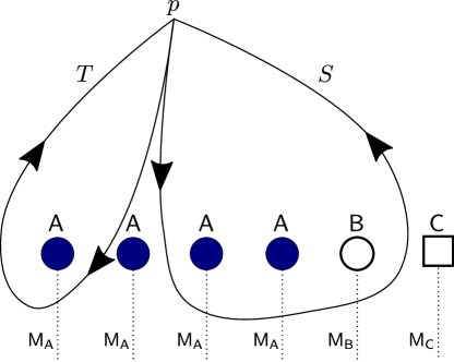
Figure 5: The paths that implement the monodromies $S$ and $T$ at the point $p$ in the presence of the degenerations of the elliptic fibration discussed in the text. The dotted lines indicate branch cuts. The monodromies indicated in the text are obtained by crossing the branch cut counterclockwise.

We now specialize to the $A_{2}$ theory, for concreteness, the generalization to other algebras being clear. Thus, we aim to describe an $\mathcal{N}=4$ theory with algebra $\mathfrak{su}(3)$ on $\mathbb{P}^{1}\times\Sigma$ in the presence of duality defects. What is the global form of the gauge group of this theory? Intriguingly, this question is not answerable, because none of the genuine $\mathfrak{su}(3)$ theories can be placed in a background with generic duality defects. This because these theories are not invariant under the $SL(2,\mathbb{Z})$ monodromy group of a generic collection of defects, see figure 6. More concretely, say that we declare that the gauge group on a $\mathbb{R}^{4}$ neighbourhood of the point $p$ in figure 5 is of the form $SU(3)$. By taking the path with monodromy $\tau\to-1/\tau$, we end up with $(SU(3)/\mathbb{Z}_{3})_{0}$ instead, in contradiction with our initial assertion.

Figure 6: $SL(2,\mathbb{Z})$ duality orbits for the $\mathcal{N}=4$ $\mathfrak{su}(3)$ theories, from Aharony:2013hda .

There are two kinds of solutions to this problem. More conservatively, we can restrict to some particular genuine theory, which will restrict to a particular class of duality defects leaving the choice of theory invariant. While this is well suited to certain problems, this restrictive viewpoint is not always satisfactory. For instance, the 6d viewpoint suggests the possibility of a 4d/4d correspondence between duality defects on $\mathbb{P}^{1}\times\Sigma$ and elliptically fibered $\mathrm{K3}$ with constant gauge coupling. However, if we fix a choice of genuine theory in the former case, then the boundary conditions will not be invariant under large diffeomorphisms of $\mathrm{K3}$ in the latter, whereas they will be invariant under large diffeomorphisms of $\Sigma$.

This suggests a second solution, which is to view the 4d theory with varying $\tau$ as a kind of metatheory, just like the $(2,0)$ theory. In classifying general boundary conditions, we are led back to the Heisenberg group

$$0\to U(1)\to\mathcal{W}_{3}\to H^{3}(\mathrm{K3}\times\Sigma;\mathbb{Z}_{3})\to 0\,,$$ (116)

arising from the 6d perspective. However, in some cases it is interesting to focus on more restricted choices other than those arising from genuine 4d theories. For instance, as we have seen above, it is particularly natural to consider choices that are invariant under large diffeomorphisms of $\Sigma$. We discuss a further motivation for $\Sigma$-independent boundary conditions in §4.3 below.

Does $\mathcal{W}_{3}$ contain a maximal isotropic subspace that is invariant under the large diffeomorphisms of $\Sigma$? It is a non-trivial result, shown below, that such a subspace does exist, not just for the $\mathfrak{su}(3)$ theory on $\mathrm{K3}$ but for any $(2,0)$ theory on any smooth, compact, Spin manifold $\mathcal{M}_{4}$ without torsion.

4.2 Self-dual subspaces for smooth Spin four-manifolds

If $\mathcal{M}_{4}$ has no torsion, then (cf. (86)):

$$H^{3}(\mathcal{M}_{4}\times\Sigma;\Gamma^{\text{ab}})=H^{3}(\mathcal{M}_{4};\Gamma^{\text{ab}})\oplus[H^{2}(\mathcal{M}_{4};\Gamma^{\text{ab}})\otimes H^{1}(\Sigma)]\oplus H^{1}(\mathcal{M}_{4};\Gamma^{\text{ab}})\,.$$ (117)

Thus, a $\Sigma$-independent maximal isotropic subspace of $H^{3}(\mathcal{M}_{4}\times\Sigma;\Gamma^{\text{ab}})$ should take the form

$$L=L^{3}\oplus(L^{2}\otimes H^{1}(\Sigma))\oplus L^{1}\,,\qquad L^{2}=(L^{2})^{\perp}\,,\qquad L^{3}=(L^{1})^{\perp}\,,$$ (118)

where $L^{i}\subseteq H^{i}(\mathcal{M}_{4};\Gamma^{\text{ab}})=H^{i}(\mathcal{M}_{4})\otimes H^{2}(S^{3}/\Gamma)$ and $(\ldots)^{\perp}$ denotes the orthogonal complement with respect to the linking pairing

$$\mathsf{L}_{\mathcal{M}_{4}}(a_{1}\otimes\ell_{1},a_{2}\otimes\ell_{2})=(a_{1}\circ a_{2})\mathsf{L}_{\Gamma}(\ell_{1},\ell_{2})\,,$$ (119)

with $a_{1}\circ a_{2}=\int_{\mathcal{M}_{4}}a_{1}\smile a_{2}$ the intersection form on $\mathcal{M}_{4}$.

Note that the linking pairing $\mathsf{L}_{\mathcal{M}_{4}}$ is symmetric. Following the nomenclature of §3.2, we call a subspace $L$ of the form $L=L^{\perp}$ “self-dual”, where in particular this differs from a maximal isotropic subspace (applicable to an antisymmetric linking pairing) in that a self-dual subspace is not guaranteed to exist. Because we can freely pick $L^{1}$, fixing $L^{3}=(L^{1})^{\perp}$ (or vice versa), the existence of a $\Sigma$-independent maximal isotropic subspace of $H^{3}(\mathcal{M}_{4}\times\Sigma;\Gamma^{\text{ab}})$ is equivalent to the existence of a self-dual subspace of $H^{2}(\mathcal{M}_{4};\Gamma^{\text{ab}})$. Below, we show that such a subspace exists for any smooth, compact Spin manifold $\mathcal{M}_{4}$ without torsion and for any $\Gamma$.

4.2.1 The $\mathfrak{su}(2)$ case

We begin with the $A_{1}$ case, deferring a general statement till later. As above, we assume that $\mathcal{M}_{4}$ is compact, Spin, and without torsion. Additionally, in order to be able to apply some general results of Donaldson, we require that $\mathcal{M}_{4}$ is smooth.

Since $\mathcal{M}_{4}$ is torsion-free, $H^{i}(\mathcal{M}_{4};\mathbb{Z}_{2})=H^{i}(\mathcal{M}_{4})\otimes\mathbb{Z}_{2}$. Denote by $\rho\colon H^{i}(\mathcal{M}_{4})\to H^{i}(\mathcal{M}_{4};\mathbb{Z}_{2})$ the associated mod-2 reduction of cohomology classes. Explicitly, $\rho$ is constructed from the short exact sequence

$$0\to\mathbb{Z}\xrightarrow{\times 2}\mathbb{Z}\xrightarrow{\text{mod}\ 2}\mathbb{Z}_{2}\to 0\,,$$ (120)

which induces the long exact sequence in cohomology

$$\ldots\to H^{2}(\mathcal{M}_{4})\xrightarrow{\psi}H^{2}(\mathcal{M}_{4})\xrightarrow{\rho}H^{2}(\mathcal{M}_{4};\mathbb{Z}_{2})\xrightarrow{\phi}H^{3}(\mathcal{M}_{4})\to\cdots$$ (121)

Since there is no torsion in $\mathcal{M}_{4}$ the map $\phi=0$ in (121) is necessarily vanishing, and then $H^{2}(\mathcal{M}_{4};\mathbb{Z}_{2})\cong\operatorname{coker}(\psi)$. Since $\psi$ is simply multiplication of elements in $H^{2}(\mathcal{M}_{4})$ by 2, we can write

$$H^{2}(\mathcal{M}_{4};\mathbb{Z}_{2})=\frac{H^{2}(\mathcal{M}_{4})}{2H^{2}(\mathcal{M}_{4})}\,,$$ (122)

and think of elements of $H^{2}(\mathcal{M}_{4};\mathbb{Z}_{2})$ as the reduction modulo 2 of elements in $H^{2}(\mathcal{M}_{4})$.

For any $x\in H^{2}(\mathcal{M}_{4})$ we have

$$x^{2}=\rho(x)^{2}=\mathrm{Sq}^{2}(x)=\nu_{2}\circ x\mod 2$$ (123)

where $\mathrm{Sq}^{2}(x)$ denotes the Steenrod square Hatcher:478079 and $\nu_{2}$ is the second Wu class spanier , which in terms of Stiefel-Whitney classes can be written as $\nu_{2}=w_{2}+w_{1}^{2}$. A Spin manifold has $w_{1}=w_{2}=0$, so we learn that the intersection form is even. A theorem of Donaldson donaldson1983 ; donaldson1987 then implies that the intersection form is necessarily of indefinite signature.

Likewise, the intersection form is unimodular when $\mathcal{M}_{4}$ is compact. The classification of even unimodular forms of indefinite signature is a classical result, known as the Hasse-Minkowski classification (see MilnorHusemoller ), implying that one can choose a basis for $H^{2}(\mathcal{M}_{4})$ such that the intersection form is given by a block diagonal matrix of the form

$$(-C(E_{8}))^{\oplus p}\oplus H^{\oplus q}\,.$$ (124)

Here $p\geq 0$ and $q>0$ are integers depending on $\mathcal{M}_{4}$, $H$ is the matrix

$$H=\begin{pmatrix}0&1\\ 1&0\end{pmatrix}\,,$$ (125)

and $-C(E_{8})$ is the negative of the Cartan matrix of $E_{8}$, which in our conventions will be written

$$C(E_{8})=\begin{pmatrix}2&0&-1&0&0&0&0&0\\ 0&2&0&-1&0&0&0&0\\ -1&0&2&-1&0&0&0&0\\ 0&-1&-1&2&-1&0&0&0\\ 0&0&0&-1&2&-1&0&0\\ 0&0&0&0&-1&2&-1&0\\ 0&0&0&0&0&-1&2&-1\\ 0&0&0&0&0&0&-1&2\end{pmatrix}\,.$$ (126)

We would like to construct a $\mathbb{Z}_{2}$-symplectic structure on $\mathcal{M}_{4}$, by which we mean a choice of basis for $H^{2}(\mathcal{M}_{4};\mathbb{Z}_{2})$ such that the $\mathbb{Z}_{2}$ valued intersection form in this basis has the form $H^{\oplus(4p+q)}$. Clearly, the problem reduces to finding a change of basis for each $C(E_{8})$ block. The $\mathbb{Z}_{2}$-valued intersection form on $H^{2}(\mathcal{M}_{4};\mathbb{Z}_{2})$ is defined in terms of that on $H^{2}(\mathcal{M}_{4})$ by

$$a\cdot b\equiv\hat{a}\circ\hat{b}\pmod{2}\,,$$ (127)

where for conciseness we have denoted $\hat{a}=\rho^{-1}(a)$ and $\hat{b}=\rho^{-1}(b)$ for the uplifts to $H^{2}(\mathcal{M}_{4})$. Likewise, there is a quadratic refinement $(\cdot)^{2}/2:H^{2}(\mathcal{M}_{4};\mathbb{Z}_{2})\to\mathbb{Z}_{2}$ (the Pontryagin square) given by

$$a^{2}/2\equiv(\hat{a}\circ\hat{a})/2\pmod{2}\,.$$ (128)

As discussed above, the intersection form is even, so $a^{2}/2\in\mathbb{Z}_{2}$ as required. While we are primarily interested in the intersection form, the Pontryagin square shows up in certain calculations (see (96) and Aharony:2013hda ), so we will keep track of it as well. In particular, the symplectic basis can be chosen so that $a^{2}/2=0$ for each basis element $a$.

We now explicitly construct a $\mathbb{Z}_{2}$-symplectic basis for the $C(E_{8})$ intersection form. Denote by $\hat{e}_{i}$ the generators of $H^{2}(\mathcal{M}_{4})$ with $\hat{e}_{i}\cdot\hat{e}_{j}=-C(E_{8})_{ij}$ as above. They define an associated basis $\{e_{i}\}$ of $H^{2}(\mathcal{M}_{4};\mathbb{Z}_{2})$, by taking $e_{i}=\rho(\hat{e}_{i})$. The desired symplectic basis is given by $s_{i}=S_{ij}e_{j}$ with

$$S=\begin{pmatrix}1&1&1&0&1&0&1&1\\ 0&1&1&0&1&0&1&1\\ 1&1&0&1&0&0&0&0\\ 1&0&0&1&0&0&0&0\\ 0&1&0&0&1&0&0&0\\ 0&1&0&0&1&1&0&0\\ 1&1&0&0&1&0&1&0\\ 1&0&0&0&0&0&0&1\end{pmatrix}\,.$$ (129)

Consider the lift $\hat{s}_{i}=S_{ij}\hat{e}_{j}$. We have

$$\hat{s}_{i}\cdot\hat{s}_{j}=-(SC(E_{8})S^{t})_{ij}=-\begin{pmatrix}8&7&0&-2&4&2&6&2\\ 7&8&-2&-4&4&2&4&0\\ 0&-2&4&3&0&0&2&2\\ -2&-4&3&4&-2&-2&0&2\\ 4&4&0&-2&4&3&4&0\\ 2&2&0&-2&3&4&2&0\\ 6&4&2&0&4&2&8&1\\ 2&0&2&2&0&0&1&4\end{pmatrix}_{ij}\,.$$ (130)

Reducing modulo 2, we conclude that

$$s_{i}\cdot s_{j}=(H^{\oplus 4})_{ij}\,.$$ (131)

Since the diagonal elements are likewise multiples of four, $s_{i}^{2}/2=0$, and we are done.

4.2.2 $SL(2,\mathbb{Z})$-invariant partition function on $\mathrm{K3}$

The symplectic basis we have just constructed yields a self-dual subspace $\mathcal{I}_{0}$ of $H^{2}(\mathcal{M}_{4};\mathbb{Z}_{2})$ in a rather trivial manner: divide the generators $s_{i}$ into pairs $(e_{i},\bar{e}_{i})$, with the property that $e_{i}\cdot e_{j}=\bar{e}_{i}\cdot\bar{e}_{j}=0$ and $e_{i}\cdot\bar{e}_{j}=\delta_{ij}$. Then $\mathcal{I}_{0}=\operatorname{Span}\{e_{1},\ldots,e_{n}\}$ is self-dual, where $n=4p+q$ and $|\mathcal{I}_{0}|=2^{n}$. There are many such subspaces because, e.g., we can exchange $e_{1}\leftrightarrow\bar{e}_{1}$, and likewise for the other pairs. Note that $\mathcal{I}_{0}$ is also “null”, which we define to mean $x^{2}/2=0$ for all $x\in\mathcal{I}_{0}$. Self-dual does not imply null, since, e.g., $\operatorname{Span}\{e_{1}+\bar{e}_{1},\ldots,e_{n}+\bar{e}_{n}\}$ is self-dual but not null. This distinction makes a difference for some calculations.

Letting $\mathcal{M}_{4}$ be simply connected for simplicity (so as to be able to ignore $L^{1,3}$ in (118)), corresponding to the self-dual subspace $\mathcal{I}_{0}$ there is a maximal isotropic subspace

$$L_{0}=\mathcal{I}_{0}\otimes H^{1}(\Sigma)\subset H^{3}(\mathcal{M}_{4}\times\Sigma)\,.$$ (132)

The associated choice of boundary conditions is invariant under large diffeomorphisms of $\Sigma$, as desired, but not under large diffeomorphisms of $\mathcal{M}_{4}$.

We now perform some checks on this construction. Consider type IIB string theory on $\mathcal{M}_{4}\times T^{2}\times\mathbb{C}^{2}/\mathbb{Z}_{2}$ with the boundary condition $\left|L_{0}\right\rangle$ associated to the maximal isotropic subspace $L_{0}$ in (132). Since $L_{0}$ is invariant under large diffeomorphisms of $T^{2}$, in the small $T^{2}$ limit we expect to obtain an effective 4d description on $\mathcal{M}_{4}$ that is $SL(2,\mathbb{Z})$ invariant. For concreteness, choose $\mathcal{M}_{4}=\mathrm{K3}$, which should give a four dimensional $\mathcal{N}=4$ theory with algebra $\mathfrak{su}(2)$ on $\mathrm{K3}$, with a peculiar choice of global structure that is not invariant under large diffeomorphisms of the $\mathrm{K3}$, but is invariant under the $SL(2,\mathbb{Z})$ duality group of $\mathcal{N}=4$ $\mathfrak{su}(2)$ theory. We will refer to this choice of global structure as $SO(3)_{0}$. We emphasize that in contrast to genuine 4d field theories, but reflecting its origin in the $(2,0)$ theory of type $A_{1}$ (equivalently from the IIB $\mathbb{C}^{2}/\mathbb{Z}_{2}$ orbifold), the construction of this “theory” makes explicit reference to the topology of $\mathcal{M}_{4}$ in the form of a particular choice of self-dual $\mathcal{I}$, which is not invariant under large diffeomorphisms of $\mathcal{M}_{4}$. Note that by the 4d/4d correspondence discussed above, this theory is related to one with 24 duality defects on $\mathbb{P}^{1}\times T^{2}$ where invariance under large diffeomorphisms has been imposed along the $T^{2}$. The existence of self-dual $\mathcal{I}$ is a non-trivial check (at the level of the partition function) that this is possible.

To proceed further, we write $\left|L_{0}\right\rangle$ in a particular basis, which will give an expansion of the partition function $Z(\tau)=\bigl{\langle}Z|L_{0}\bigr{\rangle}$ in terms of “conformal blocks.” A convenient choice is the one associated to the ordinary $SU(2)$ theory, with basis elements $\left|v\right\rangle$ for each $v\in H^{2}(\mathcal{M}_{4};\mathbb{Z}_{2})$, each associated to a background flux $v$ for the $\mathbb{Z}_{2}$ one-form symmetry of the theory. Equivalently, as in Vafa:1994tf , we can think of the basis elements $\left|v\right\rangle$ as representing classes of $SO(3)$ gauge bundles that are not $SU(2)$ gauge bundles. Referring to §2.1, §3.4 we see that

$$\Phi_{u\otimes a}\left|v\right\rangle=(-1)^{u\cdot v}\left|v\right\rangle\,,\qquad\Phi_{u\otimes b}\left|v\right\rangle=\left|u+v\right\rangle\,,$$ (133)

where $a,b$ denote the generators of the $A$ and $B$ cycles of $T^{2}$ and we fix the phases of the basis elements so that $\left|v\right\rangle=\Phi_{v\otimes b}\left|0\right\rangle$.

The associated conformal blocks $Z_{v}(\tau)=\bigl{\langle}Z|v\bigr{\rangle}$ were computed by Vafa and Witten Vafa:1994tf . We will not need the precise expressions, only their transformations under $SL(2,\mathbb{Z})$, which are given below. By linearity, given $Z_{v}(\tau)$ we can determine the partition function for the $SO(3)_{0}$ theory on $\mathrm{K3}$ once we decompose $\left|L_{0}\right\rangle$ in the $\{\left|v\right\rangle\}$ basis. To do so, recall that the defining property of $\left|L_{0}\right\rangle$ is that

$$\Phi_{x}\left|L_{0}\right\rangle=\left|L_{0}\right\rangle$$ (134)

for all $x\in L_{0}=\mathcal{I}_{0}\otimes H^{1}(T^{2})$. Since $\{\left|v\right\rangle\}$ is a basis, we can write

$$\left|L_{0}\right\rangle=\sum_{v}c_{v}\left|v\right\rangle$$ (135)

for some $c_{v}$ to be determined. We have $L_{0}=L_{0}^{(a)}\oplus L_{0}^{(b)}$ where $L_{0}^{(a)}\coloneqq\mathcal{I}_{0}\otimes a$ and $L_{0}^{(b)}\coloneqq\mathcal{I}_{0}\otimes b$ with $a,b$ the generators of $H^{1}(T^{2})$, so if (134) holds for $L_{0}^{(a)}$ and $L_{0}^{(b)}$ then it holds for all $L_{0}$. Thus, we require

$$\Phi_{a\otimes u}\left|L_{0}\right\rangle =\sum_{v}c_{v}(-1)^{u\cdot v}\left|v\right\rangle=\left|L_{0}\right\rangle, \Phi_{b\otimes u}\left|L_{0}\right\rangle =\sum_{v\in\mathcal{I}_{0}}c_{v}\left|u+v\right\rangle=\left|L_{0}\right\rangle,$$ (136)

for all $u\in\mathcal{I}_{0}$. The first condition implies that

$$c_{v}(-1)^{u\cdot v}=c_{v}\,,\qquad\forall u\in\mathcal{I}_{0}\,.$$ (137)

Since $\mathcal{I}_{0}$ is self-dual, this implies that $c_{v}=0$ for $v\notin\mathcal{I}_{0}$. The second condition then implies $c_{v}=c_{v}^{\prime}$ for $v,v^{\prime}\in\mathcal{I}_{0}$, so we conclude that

$$\left|L_{0}\right\rangle=\sum_{v\in\mathcal{I}_{0}}\left|v\right\rangle\,,$$ (138)

up to an overall normalization that we will not fix carefully. The partition function for $SO(3)_{0}$ is therefore

$$Z_{SO(3)_{0}}(\tau)=\sum_{v\in\mathcal{I}_{0}}Z_{v}(\tau)\,.$$ (139)

According to the results in Vafa:1994tf , under S-duality we have

$$Z_{v}(-1/\tau)=(-1)^{\frac{\chi(\mathrm{K3})+\sigma(\mathrm{K3})}{4}}2^{-n}\left(\frac{\tau}{i}\right)^{-\frac{\chi(\mathrm{K3})}{2}}\sum_{u\in H^{2}(\mathcal{M}_{4};\mathbb{Z}_{2})}(-1)^{u\cdot v}Z_{u}(\tau)\,,$$ (140)

with $\chi(\mathrm{K3})=24$ and $\sigma(\mathrm{K3})=-16$ the Euler characteristic and signature of $\mathrm{K3}$, and $n=11$ so that $\dim(H^{2}(\mathcal{M}_{4}))=2n$ as above. Likewise,

$$Z_{v}(\tau+1)=(-1)^{v^{2}/2}Z_{v}(\tau)\,,$$ (141)

in agreement with the general discussion in §3.5.

We now check how $Z_{0}(\tau)$ transforms under $SL(2,\mathbb{Z})$. Invariance under $T$ is immediate, since $\mathcal{I}_{0}$ is null. To derive the $S$-transformation, we use

$$\sum_{v\in\mathcal{I}_{0}}(-1)^{u\cdot v}=\begin{cases}2^{n}&\text{if }u\in\mathcal{I}_{0}\,,\\ 0&\text{if }u\notin\mathcal{I}_{0}\,.\end{cases}$$ (142)

The case $u\in\mathcal{I}_{0}$ is immediate. When $u\notin\mathcal{I}_{0}$, $\mathcal{I}_{0}$ can be divided into cosets $\mathcal{I}_{u}$ and $\mathcal{I}_{u}+v_{u}$, where $\mathcal{I}_{u}=\{v\in\mathcal{I}_{0}|u\cdot v=0\}$ and $v_{u}$ is any element of $\mathcal{I}_{0}-\mathcal{I}_{u}$ (so that $(-1)^{u\cdot v_{u}}=-1$). The cosets are of equal size $2^{n-1}$, so the positive and negative terms in the sum cancel. Using (140) and (142), we immediately conclude that

$$Z_{SO(3)_{0}}(-1/\tau)=\tau^{-12}Z_{SO(3)_{0}}(\tau)\,.$$ (143)

As explained in Vafa:1994tf , the fact that the partition function is a modular form of non-zero weight originates from omitting higher derivative couplings to the curvature. We obtain a fully modular invariant function by multiplying by, e.g., $\eta(\tau)^{24}$. Something similar should correspond to including the appropriate higher derivative terms in the calculation.

One can perform a similar analysis of the modular properties of the $\mathrm{K3}$ partition function for $\mathfrak{su}(N)$ theories. We leave the technical details to appendix B, but note that the results are in perfect agreement with the type IIB viewpoint developed above as well as with Aharony:2013hda . For the present, we confine ourselves to the question of the existence of self-dual $\mathcal{I}_{0}$ in the $\mathfrak{su}(N)$ case (and for other algebras), as discussed below.

4.2.3 $\mathfrak{su}(N)$ and other algebras

It is not difficult to extend the argument of §4.2.1 from $\mathfrak{su}(2)$ to $\mathfrak{su}(N)$ for small values of $N$ by brute force, but the computation quickly gets unwieldy. Luckily, the mathematical problem that we are studying has a well known general solution. Abstractly, what we are trying to show is that the Cartan matrix $C(E_{8})$ in (126) and $H^{\oplus 4}$ are equivalent as bilinear forms over $\mathbb{Z}_{N}$. This is certainly not true over $\mathbb{Z}$, as $C(E_{8})$ and $H^{\oplus 4}$ have different signatures, $(8,0)$ and $(4,4)$ respectively. However, the signature is not well-defined over $\mathbb{Z}_{N}$, and so with no obvious invariant to distinguish them, it perhaps unsurprising that $C(E_{8})$ and $H^{\oplus 4}$ become equivalent. In fact, we will see that any two even unimodular bilinear forms of the same dimension become equivalent over $\mathbb{Z}_{N}$.

To show this, note that by the Chinese remainder theorem

$$\mathbb{Z}_{N}=\mathbb{Z}_{p_{1}^{n_{1}}}\oplus\cdots\oplus\mathbb{Z}_{p_{k}^{n_{k}}}\,,$$ (144)

where $N=p_{1}^{n_{1}}\cdots p_{k}^{n_{k}}$ and the $p_{i}$ are distinct prime numbers. Given a change of basis from $C(E_{8})$ to $H^{\oplus 4}$ modulo $N_{i}=p_{i}^{n_{i}}$ for each factor, we can again use the Chinese remainder theorem to assemble them into a change of basis over $N$. Thus, we can set $N=p^{n}$ for the rest of the proof without loss of generality.

We first consider the case of $p\neq 2$. We introduce the Jacobi-Legendre symbol for $a\in\mathbb{Z}$ and prime $p$, defined as

$$\left(\frac{a}{p}\right)=\begin{cases}1&\text{if $a$ is a quadratic residue mod $p$ and $a\mathrel{\not\equiv}0\bmod p$},\\ -1&\text{if $a$ is not a quadratic residue mod $p$,}\\ 0&\text{otherwise.}\end{cases}$$ (145)

Then theorem 9 in section 15.7.2 of ConwaySloane implies that two quadratic forms $f$ and $g$ are equivalent over $\mathbb{Z}_{p^{n}}$ if and only if they have the same dimensions and

$$\left(\frac{\det f}{p}\right)=\left(\frac{\det g}{p}\right)\,.$$ (146)

Since we have that both $\det(H^{\oplus 4})=\det(C(E_{8}))=1$, it follows that these bilinear forms (or more generally, any two unimodular forms) are equivalent modulo $p^{n}$ for any $n>0$ and any prime $p>2$.

The case $p=2$ is addressed in theorem 10 in section 15.7.5 of ConwaySloane . This theorem implies that even bilinear forms are equivalent over $2^{n}$ iff the same conditions as above hold, namely that they have the same dimension and the same Jacobi-Legendre symbol

$$\left(\frac{\det f}{2}\right)=\left(\frac{\det g}{2}\right)\,.$$ (147)

As above, this is clearly satisfied for $C(E_{8})$ and $H^{\oplus 4}$, as they are both even unimodular.

Thus, $C(E_{8})$ and $H^{\oplus 4}$ are equivalent bilinear forms modulo $N$ for any integer $N$. Note, however, that per (96) the partition function depends not just on the intersection form but also on its quadratic refinement, the Pontryagin square. Fortunately, in the torsion-free case that we are studying the quadratic refinement over $\mathbb{Z}_{N}$ can be extracted from the intersection form over $\mathbb{Z}_{2N}$, and so the above argument implies that the quadratic refinements of $C(E_{8})$ and $H^{\oplus 4}$ are likewise equivalent over $\mathbb{Z}_{N}$ for any $N$. In particular, since the above argument does not depend on the details of $C(E_{8})$ and $H^{\oplus 4}$, any even unimodular bilinear form admits a basis of the form

$$e_{i}\cdot e_{j}=\bar{e}_{i}\cdot\bar{e}_{j}=0\,,\qquad e_{i}\cdot\bar{e}_{j}=\delta_{ij}\,,\qquad e_{i}^{2}/2=\bar{e}_{i}^{2}/2=0\,,$$ (148)

upon reduction modulo $N$. From this, we can construct a null, self-dual subspace for $\mathfrak{su}(N)$ compactified on any smooth, compact, Spin $\mathcal{M}_{4}$ without torsion,

$$\mathcal{I}_{0}=\operatorname{Span}\{e_{i}\}\,,$$ (149)

just as in the case $N=2$ discussed above.

We briefly comment on the $(2,0)$ theories of $D$ and $E$ type. In the cases $D_{2k+1}$ and $E_{k}$, the defect group is cyclic, and the above analysis remains valid. For the $D_{4k+2}$ theory, the basis (148) for $N=2$ leads to a larger basis

$$\alpha_{i}\cdot\bar{\alpha}_{j}=\delta_{ij},\qquad\beta_{i}\cdot\bar{\beta}_{j}=\delta_{ij}\,,\qquad\alpha_{i}^{2}/2=\bar{\alpha}_{i}^{2}/2=\beta_{i}^{2}/2=\bar{\beta}_{i}^{2}/2=0\,,$$ (150)

with $\alpha_{i}=e_{i}\otimes\alpha$, $\beta_{i}=e_{i}\otimes\beta$, etc., where $\alpha$ and $\beta$ are the generators of the $\mathbb{Z}_{2}\oplus\mathbb{Z}_{2}$ defect group. Likewise, for $D_{4k}$ we obtain

$$\alpha_{i}\cdot\bar{\beta}_{j}=\delta_{ij},\qquad\beta_{i}\cdot\bar{\alpha}_{j}=\delta_{ij}\,,\qquad\alpha_{i}^{2}/2=\bar{\alpha}_{i}^{2}/2=\beta_{i}^{2}/2=\bar{\beta}_{i}^{2}/2=0\,.$$ (151)

In either case, the expanded basis is still of the form (148) for $N=2$ (with twice as many generators), and so a null self-dual subspace exists as before.

While we expect that similar statements can be made for any defect group and linking pairing, we defer further consideration of this to a future work.

4.3 2d/4d correspondences and Hecke transforms

There is another application of the previous discussion that we will now briefly outline. Consider a compactification of the $(2,0)$ theory of type $\mathfrak{g}_{\Gamma}$ on $\mathcal{M}_{6}=\mathcal{M}_{4}\times\Sigma$. There are two natural limits to take: we can take the limit in which $\Sigma$ is small, obtaining an effective four-dimensional theory $\mathcal{T}_{\Sigma}$ on $\mathcal{M}_{4}$, or alternatively we can first make $\mathcal{M}_{4}$ small, obtaining a two-dimensional theory $\mathcal{T}_{\mathcal{M}_{4}}$ on $\Sigma$. There are deep relations between $\mathcal{T}_{\mathcal{M}_{4}}$ and $\mathcal{T}_{\Sigma}$, due to their common six-dimensional origin. It is expected that such a 2d/4d correspondence exists for any suitable $\mathcal{M}_{4}$/$\Sigma$ pair, as long as we can introduce appropriate supersymmetric twists.

A basic observable that we can compute in these theories is the partition function. The expectation is that

$$Z^{\Gamma}_{(2,0)}[\mathcal{M}_{4}\times\Sigma;L]=Z_{\mathcal{T}_{\Sigma}}[\mathcal{M}_{4}]=Z_{\mathcal{T}_{\mathcal{M}_{4}}}[\Sigma]$$ (152)

where the first term denotes the partition function of the six-dimensional $(2,0)$ theory of type $\Gamma$ on $\mathcal{M}_{4}\times\Sigma$, with a choice of maximal isotropic subspace $L\subset\mathcal{W}_{3}$. Although we have chosen not to display it to avoid cluttering the notation too much, $\mathcal{T}_{\mathcal{M}_{4}}$ and $\mathcal{T}_{\Sigma}$ will depend on the choice of $L$ and $\Gamma$.

An important subtlety now arises: to obtain a genuine 4d theory, we should choose $L$ to be independent of the details of $\mathcal{M}_{4}$. Likewise, to obtain a genuine (i.e., modular invariant) 2d theory, we should choose $L$ to be independent of the details of $\Sigma$. However, we have seen that in general $L$ cannot simultaneously be invariant under large diffeomorphisms of both $\mathcal{M}_{4}$ and $\Sigma$! In particular, this is only seems to be possible when the corresponding $(2,0)$ theory is genuine, see §3.2. Thus, to make (152) true we must either choose a genuine $(2,0)$ theory — and the associated $\Sigma$ and $\mathcal{M}_{4}$ reductions — or at least one of $\mathcal{T}_{\mathcal{M}_{4}}$ and $\mathcal{T}_{\Sigma}$ cannot be genuine.

In this section, we will explore the consequences of making the 2d theory $\mathcal{T}_{\mathcal{M}_{4}}$ genuine (modular invariant). To do so, we choose a maximal isotropic subspace of the form (118), just as above. In particular, fixing $\mathcal{M}_{4}=\mathrm{K3}$ and choosing a self-dual subspace $\mathcal{I}_{0}$ of the form (149) leads to a modular-invariant 2d CFT $\mathcal{K}_{\Gamma}$ on $\Sigma$. We have not identified this theory, but we will be able to prove some interesting facts about its elliptic genus (as defined by the Vafa-Witten partition function Minahan:1998vr ).

Choose, for concreteness, $\Gamma=\mathbb{Z}_{2}$. We denote by $\mathcal{K}_{2}\coloneqq\mathcal{K}_{\mathbb{Z}_{2}}$ the two-dimensional modular invariant theory that we are after. In this case (152) implies that

$$Z_{\mathcal{K}_{2}}[T^{2}]=Z_{SO(3)_{0}}[\mathrm{K3}]$$ (153)

see (139). It is interesting to compute this explicitly using the results of Vafa:1994tf . In particular, from a general partition vector

$$\left|L\right\rangle=\sum_{v}c_{v}\left|v\right\rangle$$ (154)

we obtain

$$Z[\mathrm{K3}]=c_{0}\hat{Z}(\tau)+c_{\text{even}}Z_{\text{even}}(\tau)+c_{\text{odd}}Z_{\text{odd}}(\tau)\,,\qquad c_{\text{even}}=\sum_{\begin{subarray}{c}v\neq 0\\ v^{2}/2=0\end{subarray}}c_{v}\,,\qquad c_{\text{odd}}=\sum_{v^{2}/2=1}c_{v}\,,$$ (155)

since the conformal blocks $Z_{v}=\{\hat{Z},Z_{\text{even}},Z_{\text{odd}}\}$ only depend on whether $v$ is zero, non-zero and even, or odd, with Vafa:1994tf

$$\hat{Z}(\tau) =\frac{1}{4}G(q^{2})+\frac{1}{2}\left[G(q^{1/2})+G(-q^{1/2})\right]\,,$$ (156a)

$$Z_{\text{even}}(\tau) =\frac{1}{2}\left[G(q^{1/2})+G(-q^{1/2})\right]\,,$$ (156b)

$$Z_{\text{odd}}(\tau) =\frac{1}{2}\left[G(q^{1/2})-G(-q^{1/2})\right]\,.$$ (156c)

where $q=\exp(2\pi i\tau)$ and

$$G(q)\coloneqq\frac{1}{\eta^{24}(q)}=\frac{1}{q\prod_{n=1}^{\infty}(1-q^{n})^{24}}\,.$$ (157)

Note that this is the elliptic genus for 24 left moving bosons, excluding their zero modes.

As a warmup, we describe the partition function for the genuine 4d $\mathfrak{su}(2)$ theories on $\mathrm{K3}$, following the nomenclature of Aharony:2013hda . For $SU(2)$, we have $c_{v}=(1/2)\delta_{v,0}$, where overall $1/2$ follows the conventions of Vafa:1994tf . By comparison, for $SO(3)_{+}$ theory, we have $c_{v}=1$, implying that $c_{\text{even}}=n_{\text{even}}$ and $c_{\text{odd}}=n_{\text{odd}}$ where $n_{\text{even}}=\frac{1}{2}(2^{22}+2^{11})-1$ and $n_{\text{odd}}=\frac{1}{2}(2^{22}-2^{11})$ count the number of non-trivial $SO(3)$ gauge bundles (see Vafa:1994tf ). Finally, for $SO(3)_{-}$ we have $c_{v}=(-1)^{v^{2}/2}$, which is the same as before except with $c_{\text{odd}}=-n_{\text{odd}}$.

We now consider the $SO(3)_{0}$ theory, as defined above. From (138), $c_{v}=\delta_{v\in\mathcal{I}_{0}}$. Since $\mathcal{I}_{0}$ is null and self-dual, this implies $c_{0}=1$, $c_{\text{even}}=2^{11}-1$, and $c_{\text{odd}}=0$, where we use $|\mathcal{I}_{0}|=2^{11}$. Thus, explicitly

$$Z_{\mathcal{K}_{2}}[T^{2}]=Z_{SO(3)_{0}}[\mathrm{K3}]=\frac{1}{4}G(q^{2})+2^{10}\left[G(q^{1/2})+G(-q^{1/2})\right]\,.$$ (158)

It is an easy exercise, using the well-known modular transformation properties of $\eta(q)$, to show that $Z_{\mathcal{K}_{2}}(\tau)$ transforms as a modular form of weight $-12$, the same as $G(q)$ itself. In fact, the two expressions are closely connected, as

$$Z_{\mathcal{K}_{2}}[T^{2}]=2^{11}(T_{2}[G])(\tau)$$ (159)

where $T_{m}$ is the Hecke operator (see SerreArithmetic ; 1-2-3-ModularForms for reviews, as well as §B.1) acting on modular forms of weight $k$ by

$$(T_{m}[f])(\tau)=m^{k-1}\sum_{\begin{subarray}{c}a,d>0\\ ad=m\end{subarray}}\frac{1}{d^{k}}\sum_{0\leq b<d}f\left(\frac{a\tau+b}{d}\right)\,.$$ (160)

In fact, the relation (159) holds more generally. Let $\mathcal{K}_{p}$ denote the theory $\mathcal{K}_{\mathbb{Z}_{p}}$ arising from the $A_{p-1}$ theory on $\mathrm{K3}$. In the case where $p$ is prime, the elliptic genus for $\mathcal{K}_{p}$ is computed in appendix B.2, with the result

$$Z_{\mathcal{K}_{p}}[T^{2}]=\frac{1}{p^{2}}G(p\tau)+p^{10}\sum_{j=0}^{p-1}G\left(\frac{\tau+j}{p}\right)\,,$$ (161)

which can be easily checked to satisfy

$$Z_{\mathcal{K}_{p}}[T^{2}]=p^{11}(T_{p}[G])(\tau)\,.$$ (162)

By a more involved calculation, this formula can also be shown to hold for composite $N$, see §B.5.

We see that, at least at the level of the elliptic genus, the set of theories $\mathcal{K}_{N}$ is in some sense generated from the theory of 24 left-moving bosons with elliptic genus $G(\tau)$. More precisely, there exists a family of modular-invariant two-dimensional conformal field theories $\mathcal{K}_{N}$, obtained by compactification of the six-dimensional $(2,0)$ theory of type $A_{N-1}$ on $\mathrm{K3}$, whose elliptic genera are

$$Z_{\mathcal{K}_{N}}[T^{2}](\tau)=f(\tau)(T_{N}[G])(\tau)\,,$$ (163)

where now we introduce a prefactor of $f(\tau)$ to account for possible (unknown) curvature corrections Vafa:1994tf . We expect these corrections to restore modular invariance, as we ultimately have a IIB compactification with boundary conditions invariant under large diffeomorphisms on $\Sigma$. Modular invariance constrains $f(\tau)$ to be a modular form of weight 12, but it is otherwise unknown. We will conjecture a specific form below.

Note that the situation is very similar to the original discussion in Minahan:1998vr , where it was show that there is a similar relation between the theory of $N$ M5 branes and the heterotic string. Namely, the partition function of $N$ M5 branes on $\mathrm{K3}\times T^{2}$ is the same as the $N$-th Hecke transform of the heterotic string partition function on $T^{2}$. While in the case of M5 branes it was natural to expect the existence of a modular invariant theory — as the $\mathcal{N}=4$ $U(N)$ theory is $SL(2,\mathbb{Z})$ invariant — the existence of the $\mathcal{K}_{N}$ theories is a bit more surprising, and crucially depends on the existence of the self-dual subspaces $\mathcal{I}_{0}$ constructed in §4.2.2. It would be very interesting to learn more about this class of theories (and their natural generalizations when we replace $\mathrm{K3}$ by other four-manifolds), particularly given their close connection to the six-dimensional $(2,0)$ theory.

A conjecture for $f(\tau)$

We now make a simple guess for $f(\tau)$, with interesting consequences. To motivate it, we make the following assumptions:

1. $f(\tau)$ is a modular form of weight 12.

2. $f(\tau)$, coming from curvature corrections, is independent of $N$.

3. The form (163) holds for $N=1$, where we expect to have a trivial theory.

These conditions, taken together, fix $f(\tau)=G^{-1}(\tau)=\eta^{24}(\tau)$, up to an overall constant which we take to be $N^{13}$ for convenience. That is, we conjecture that the full modular invariant elliptic genus is

$$Z_{\mathcal{K}_{N}}[T^{2}](\tau)=N^{13}\frac{T_{N}[G](\tau)}{G(\tau)}\,.$$ (164)

Assuming that this is indeed the case, one finds the result

$$Z_{\mathcal{K}_{2}}[T^{2}](\tau)=2^{13}\eta^{24}(\tau)(T_{2}[\eta^{-24}])(\tau)=J(\tau)-24\,,$$ (165)

where

$$J(\tau)=j(\tau)-744=\frac{1}{q}+196884q+21493760q^{2}+864299970q^{3}+\ldots$$ (166)

is Klein’s $j$-invariant without the constant term. Two dimensional theories with partition function equal to the $j$-invariant have a rich history, most notably the moonshine module constructed by Frenkel, Lepowsky and Meurman frenkel1989vertex , used by Borcherds to prove monstrous moonshine Borcherds1992 . It is quite enticing that the same function seems to appear (assuming that our guess for $f(\tau)$ is correct) in trying to understand the partition function of the $(2,0)$ $A_{1}$ theory on $\mathrm{K3}$.

From a purely mathematical point of view, we can understand the appearance of the $j$-function here from the fact that $Z_{\mathcal{K}_{N}}[T^{2}](\tau)$ is a modular function that is analytic in the upper half plane and meromorphic with a pole of order $N-1$ at $q=0$, so it can be expressed as an order $N-1$ polynomial in $J(\tau)$ for any $N$. The $N$ coefficients in the expression in terms of $J(\tau)$ can be determined by looking to the first $N$ terms in the Laurent expansion of $Z_{\mathcal{K}_{N}}[T^{2}](\tau)$ around $q=0$.

It is in fact possible to give concise expressions for the expansion of $Z_{\mathcal{K}_{N}}[T^{2}](\tau)$ in terms of $J(\tau)$ in the case that $N$ is prime, as a special case of the results in Carney2012 . Define

$$\mathcal{B}(x;q)\coloneqq\frac{E_{4}^{2}(q)E_{6}(q)}{q(j(q)-x)}\,,$$ (167)

where we have introduced the Eisenstein series $E_{4}(q)=1+240q+2160q^{2}+6720q^{3}+\ldots$ and $E_{6}(q)=1-504q-16632q^{2}-122976q^{3}+\ldots$. If we denote by $B(m;x)$ the coefficients in the $q$-expansion of $\mathcal{B}(x;q)$,

$$\mathcal{B}(x;q)\coloneqq\sum_{m=1}^{\infty}B(m;x)q^{m}\,,$$ (168)

we have that

$$Z_{\mathcal{K}_{N}}[T^{2}](\tau)=B(N-1;J(\tau)+744)\,.$$ (169)

For reference, we find the elliptic genera for the first few primes to be

$$Z_{\mathcal{K}_{2}}[T^{2}](\tau) =J(\tau)-24\,,$$

$$Z_{\mathcal{K}_{3}}[T^{2}](\tau) =J(\tau)^{2}-24J(\tau)-393516\,,$$

$$Z_{\mathcal{K}_{5}}[T^{2}](\tau) =J(\tau)^{4}-24J(\tau)^{3}-787284J(\tau)^{2}-71800864J(\tau)+75517745046\,.$$ (170)

We can also analyze directly the case of small composite $N$ by comparing coefficients in the Laurent expansion around $q=0$. In this way we find, for instance

$$Z_{\mathcal{K}_{4}}[T^{2}](\tau) =J(\tau)^{3}-24J(\tau)^{2}-590400J(\tau)-55032320\,,$$

$$Z_{\mathcal{K}_{6}}[T^{2}](\tau) =J(\tau)^{5}-24J(\tau)^{4}-984168J(\tau)^{3}-88569408J(\tau)^{2}+191409608916J(\tau)$$

$$\mathrel{\phantom{=}}\qquad+19264322219040\,.$$ (171)

Intriguingly, this agrees with (169), and it seems reasonable to conjecture that the formula is valid for all $N$.

It is also interesting to look directly to $q$ expansion in the small $N$ cases:

$$Z_{\mathcal{K}_{2}}[T^{2}](\tau) =\frac{1}{q}-24+\ldots\,,$$

$$Z_{\mathcal{K}_{3}}[T^{2}](\tau) =\frac{1}{q^{2}}-\frac{24}{q}+252+\ldots\,,$$

$$Z_{\mathcal{K}_{4}}[T^{2}](\tau) =\frac{1}{q^{3}}-\frac{24}{q^{2}}+\frac{252}{q}-1472+\ldots\,,$$

$$Z_{\mathcal{K}_{5}}[T^{2}](\tau) =\frac{1}{q^{4}}-\frac{24}{q^{3}}+\frac{252}{q^{2}}-\frac{1472}{q}+4830+\ldots\,.$$ (172)

$$\mathmakebox[\widthof{{}={}}][c]{\vdots}$$

These expressions have a remarkably simple structure, and the general result is easily guessed from here

$$Z_{\mathcal{K}_{N}}[T^{2}](\tau)=\frac{1}{q^{N}G(q)}+O(q)=\frac{1}{q^{N}}\sum_{n=1}^{\infty}q^{n}\uptau(n)+O(q)\,,$$ (173)

where $\uptau(n)$ is the Ramanujan tau function, not to be confused with the modular parameter $\tau$. Note that this form is somewhat reminiscent of extremal CFTs, see, e.g., Witten:2007kt , but with the vacuum character replaced by a different function.

In fact, (173) is easy to prove using the properties of the Hecke operator. From it, we obtain the exact expression,

$$Z_{\mathcal{K}_{N}}[T^{2}](\tau)=\sum_{n=1}^{N}\uptau(n)J_{N-n}(\tau)\,,$$ (174)

where $J_{n}(\tau)\coloneqq T_{n}[J](\tau)$ has the $q$ expansion $q^{-n}+196884q^{n}+\ldots$ for $n>0$, with $J_{0}(\tau)\coloneqq 1$.

5 Conclusions

In this paper we have shown how to understand from the IIB perspective the fact that the six-dimensional $(2,0)$ theories arising at $\mathbb{C}^{2}/\Gamma$ singularities typically do not have a partition function, but rather a vector of partition functions, in which the components mix under large diffeomorphisms. The basic observation is that non-commutativity of RR fluxes in type IIB string theory and non-commutativity of 2-form discrete flux operators in the $(2,0)$ theory are two sides of the same coin, and in fact they generate the same Heisenberg group. So the problem of choosing a specific direction in the Hilbert space of possible six-dimensional $(2,0)$ theories (that is, the space of “conformal blocks”) maps to the problem of choosing boundary conditions in the non-compact IIB space. More formally, we have shown how a theory with a non-invertible anomaly theory, the six-dimensional $(2,0)$ theory, can arise as a subsector of type IIB string theory, an anomaly-free theory.

One advantage of the IIB viewpoint is that it allows us to separate the problem of determining the behaviour of the discrete 2-form symmetries of the $(2,0)$ theory from the complicated local dynamics of the tensionless strings. Effectively, we have geometrized this sector of the problem into one involving free field theory for RR forms, solved in Freed:2006ya ; Freed:2006yc . This reformulation allows us to give simple derivations of some subtle facts in the six-dimensional theory, in particular the structure of the commutation relations for flux operators. While the answer for the $(2,0)$ theory was already known by compactification on $T^{2}$, our derivation has the virtue of easily generalizing to cases where the answer was not previously known, such as the $(1,0)$ theories.

The IIB perspective also provides a first principles approach to discussing the global structure of more exotic field theory setups, such as the theories with duality defects studied in §4, and naturally suggests a method to compute the anomalous phases of some strongly-coupled 4d theories under specific modular transformations, as conjectured in §3.5.

There are a number of interesting open questions that we have not addressed. For instance, we have assumed that $\mathcal{M}_{6}$ had no torsion. This was done only for mathematical simplicity, and it would be fact be physically quite interesting to drop this assumption. The fact that K-theory plays an important role in the IIB picture suggests that in the presence of torsion on $\mathcal{M}_{6}$ K-theory might play a role in the classification of field theories. It would be interesting to work this out in detail.

Along related lines, we have seen that in the absence of $\mathcal{M}_{6}$ torsion the IIB construction gives rise to all the global forms of the $(2,0)$ theories known from the holographic viewpoint Witten:1998wy . The presence of torsion in $\mathcal{M}_{6}$ introduces an interesting twist: the holographic classification of global forms for the $(2,0)$ theory is given in terms of cohomology in M-theory, while that for IIB is given in terms of K-theory. Comparing the results of both descriptions would be very interesting, and is potentially somewhat analogous to but different from Witten:1999vg ; Diaconescu:2000wy .

It would also be interesting to understand the results in this paper from the viewpoint of the 11d anomaly theory for IIB string theory Belov:2004ht ; Belov:2006jd ; Belov:2006xj ; Monnier:2011rk ; Monnier:2013kna . Our results suggest that in some sense non-invertible anomaly theories can be constructed by considering the behaviour of invertible anomaly theories in non-compact spaces; it would be interesting to make this statement precise. Such a reformulation would likely have useful applications in the study of duality anomalies for strongly coupled four dimensional theories, as we have sketched above.

Although we have focused mostly on $\mathrm{K3}\times\mathbb{C}^{2}/\Gamma\times T^{2}$, it is clear that the basic idea will generalize to more involved geometries. For instance, one can study the global structure in the case of Vafa-Witten topologically-twisted compactifications of $\mathcal{N}=4$ on other four-manifolds $\mathcal{M}_{4}$, such as $\mathbb{P}^{2}$, where we also know the answer for the partition function Vafa:1994tf ; Minahan:1998vr , by considering cases in which $\mathcal{M}_{4}$ appears as a submanifold of threefolds Minahan:1998vr or $G_{2}$ manifolds Bershadsky:1995qy . More generally, we might consider different theories in four dimensions, such as those coming from other choices for the 4d topological twist, or alternatively the $\Omega$-deformed backgrounds that lead to the 4d/2d correspondence found by Alday, Gaiotto and Tachikawa Alday:2009aq . (See Hellerman:2011mv ; Hellerman:2012zf for discussion on how to realize these backgrounds in string theory.)

Along similar lines, we could also consider compactifications on singular Calabi-Yau theefolds in the context of geometric engineering (starting with Klemm:1996bj ; Katz:1997eq ; Gukov:1999ya ; Shapere:1999xr , and more recently Cecotti:2010fi ; Cecotti:2011gu ; DelZotto:2011an ; DelZotto:2015rca ; Xie:2015rpa ; Chen:2016bzh ; Wang:2016yha ; Chen:2017wkw ). The global structure of any theory that can be engineered in terms of a singular threefold or fourfold with isolated singularities can in principle be obtained via an extension of the methods described here. It would be very interesting to do this in detail.

Another assumption that would be interesting to drop is that $\mathcal{M}_{6}$ is compact. We might, for instance, consider IIB on spacetimes of the form $\mathbb{C}^{2}/\Gamma_{1}\times\mathbb{C}^{2}/\Gamma_{2}\times T^{2}$. As argued in Dijkgraaf:2007sw , such a configuration leads to a chiral WZW model (with algebra determined by $\Gamma_{1}$ and $\Gamma_{2}$) living on $T^{2}$. It is natural to conjecture that a careful analysis of the boundary conditions of IIB in this background should reproduce the structure of conformal blocks of the chiral WZW model, and in particular give a geometric picture for the Verlinde formula for these theories Verlinde:1988sn ; Dijkgraaf:1988tf ; Witten:1988hf ; Moore:1988qv ; Blau:1993tv (and relatedly, a direct string theory interpretation of the work by Nakajima nakajima1994 ). Additionally, considering such non-compact geometries would be the starting point for understanding the behaviour of the global structure under gluing, along the lines of Gadde:2013sca ; Gukov:2018iiq .

The inclusion of non-simply laced algebras in lower dimensions is another important open problem. This would require the analysis of IIB backgrounds with orientifold actions, changing the type of K-theory that we need to consider.

Finally, we could also ask what happens if one replaces $\mathbb{C}^{2}/\Gamma$ by a multi-centered Taub-NUT space (for simplicity we refer to the $\Gamma=\mathbb{Z}_{N}$ case here). The local dynamics are unaffected, but there is an additional normalizable mode, corresponding to a centre of mass degree of freedom. In the six-dimensional $(2,0)$ theory this mode leads to a free tensor multiplet, which is expected to reduce in the $\mathcal{N}=4$ theory to the $U(1)$ factor of $U(N)$. In light of the results of this paper, it is natural to ask whether this is the only possibility, or one can obtain the other gauge groups with algebra $\mathfrak{u}(1)\oplus\mathfrak{su}(N)$ by choosing boundary conditions appropriately in the same IIB background. It would be interesting to work this out in detail; we expect the work of Belov and Moore Belov:2004ht ; Belov:2006jd ; Belov:2006xj to be relevant here.

Appendix A K-theory groups of $S^{3}/\Gamma$

In this appendix we compute the (complex) K-theory groups of $S^{3}/\Gamma$, with $\Gamma$ an arbitrary discrete subgroup of $U(2)$ acting freely on $S^{3}$. These spaces are orientable, with cohomology groups

$$H^{i}(S^{3}/\Gamma)=\begin{cases}\mathbb{Z}&\text{for }i\in\{0,3\}\\ \Gamma^{\text{ab}}&\text{for }i=2\\ 0&\text{for }i=1\end{cases}\,,$$ (176)

where $\Gamma^{\text{ab}}\coloneqq\Gamma/[\Gamma,\Gamma]$ denotes the abelianization of $\Gamma$, as given by the Hurewicz homomorphism. Note that $\Gamma^{\text{ab}}$ is pure torsion, since $\Gamma$ itself is.

The Atiyah-Hirzebruch spectral sequence

Say that we are interested in computing the (complex) K-theory groups $K^{p}(X)$ of some manifold $X$, where $p$ is the degree. Given that $K^{p}$ is a generalized cohomology theory (see for example §13.90 of Switzer for a description of the associated spectrum), we can compute the groups of interest using the Atiyah-Hirzebruch spectral sequence (we refer the reader to McCleary for background on the computation of spectral sequences)

$$E_{2}^{p,q}=H^{p}(X;K^{q}(\mathrm{pt}))\Rightarrow E_{\infty}^{p+q}(X)$$ (177)

associated to the fibration $0\to\mathrm{pt}\to X\to X\to 0$. Using $K^{*}(\mathrm{pt})=\mathbb{Z}[x,x^{-1}]$ and the cohomology groups (176) we can immediately write the $E_{2}$ terms in the Atiyah-Hirzebruch spectral sequence. We show the result in figure 7.

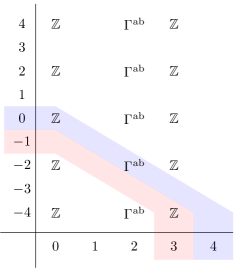
Figure 7: Contributions of the second page $E_{2}=E_{\infty}$ to $K^{0}(S^{3}/\Gamma)$ (blue, on top) and $K^{-1}(S^{3}/\Gamma)=K^{1}(S^{3}/\Gamma)$ (pink, below).

There are two small complications one encounters in going from $E_{2}$ to $K^{i}(S^{3}/\Gamma)$. First, there might be non-vanishing differentials acting on the modules in the spectral sequence. By dimensional reasons, the only potentially non-vanishing differential is

$$d_{3}\colon E_{2}^{0,p}\to E_{2}^{3,p-2}$$ (178)

for $p$ even. This differential necessarily vanishes, though, because otherwise we would find $K^{0}(S^{3}/\Gamma)=\Gamma^{\text{ab}}$, which is incompatible with the Chern homomorphism (16). The other issue to deal with is that of potential non-trivial extensions. Recall that we have

$$E_{\infty}^{p,q}=\frac{F^{p}K^{p+q}}{F^{p+1}K^{p+q}}$$ (179)

for the filtration

$$K^{n}(S^{3}/\Gamma)=F^{0}K^{n}\supset\ldots F^{i}K^{n}\supset F^{i+1}K^{n}\supset\ldots$$ (180)

The only potentially non-trivial step is

$$E_{\infty}^{0,0}=\mathbb{Z}=\frac{K^{n}(S^{3}/\Gamma)}{\Gamma^{\text{ab}}}\,,$$ (181)

or in other words that $0\to\Gamma^{\text{ab}}\to K^{n}(S^{3}/\Gamma)\to\mathbb{Z}\to 0$ is exact. But this sequence splits, since $\mathbb{Z}$ is free, and thus we find

$$K^{0}(S^{3}/\Gamma) =\mathbb{Z}\oplus\Gamma^{\text{ab}}\,, K^{1}(S^{3}/\Gamma) =\mathbb{Z}\,.$$ (182)

So in this case K-theory is completely determined by cohomology:

$$K^{i}(S^{3}/\Gamma)\cong\bigoplus_{n\equiv i\text{ mod }2}H^{n}(S^{3}/\Gamma,\mathbb{Z})\,.$$ (183)

Appendix B $\mathrm{K3}$ partition functions for $\mathcal{N}=4$ theories with algebra $\mathfrak{su}(N)$

In this appendix we perform two related calculations of the $\mathcal{N}=4$ Vafa-Witten partition function on $\mathrm{K3}$ Vafa:1994tf ; Minahan:1998vr for gauge algebra $\mathfrak{su}(N)$. Firstly, we compute the partition function for all the genuine theories classified by Aharony:2013hda , and verify that their duality relations are as expected. Secondly, we compute the elliptic genus of the modular-invariant $\mathcal{K}_{N}$ theory described in §4.3.

B.1 The Hecke operator

Before diving into the physics, we briefly review the Hecke operator and some associated identities.

Recall that a modular form $f$ of weight $w\in 2\mathbb{Z}$ is a holomorphic function satisfying

$$f\biggl{(}\frac{a\tau+b}{c\tau+d}\biggr{)}=(c\tau+d)^{w}f(\tau)$$ (184)

for any integers $a,b,c,d$ satisfying $ad-bc=1$. More generally, a non-holomorphic modular form of weight $(w,\tilde{w})$ satisfies

$$f\biggl{(}\frac{a\tau+b}{c\tau+d},\frac{a\bar{\tau}+b}{c\bar{\tau}+d}\biggr{)}=(c\tau+d)^{w}(c\bar{\tau}+d)^{\tilde{w}}f(\tau,\bar{\tau})\,.$$ (185)

where $w-\tilde{w}\in 2\mathbb{Z}$.

For any integer $m\geq 1$, we define the Hecke operator $T_{m}$ (see SerreArithmetic ; 1-2-3-ModularForms for reviews) by its action on a modular form of weight $w$

$$(T_{m}[f])(\tau)\coloneqq m^{w-1}\sum_{\begin{subarray}{c}a,d>0\\ ad=m\end{subarray}}\frac{1}{d^{w}}\sum_{0\leq b<d}f\biggl{(}\frac{a\tau+b}{d}\biggr{)}\,.$$ (186)

For a non-holomorphic modular form we replace $w\to w+\tilde{w}$.

We now show that $T_{m}[f]$ is itself a modular form of weight $w$. It is easy to see that $(T_{m}[f])(\tau+1)=(T_{m}[f])(\tau)$. To compute the $S$ transformation, we first derive a useful identity. Consider (184) with $c\neq 0$, and define $t\equiv c\tau+d$, so that $\tau=\frac{t-d}{c}$ and

$$f\biggl{(}-\frac{1}{ct}+\frac{a}{c}\biggr{)}=t^{w}f\biggl{(}\frac{t}{c}-\frac{d}{c}\biggr{)}\,.$$ (187)

Thus, for coprime $k,N$:

$$f\biggl{(}-\frac{1}{N\tau}+\frac{k}{N}\biggr{)}=\tau^{w}f\biggl{(}\frac{\tau}{N}+\frac{k^{\prime}}{N}\biggr{)}\,,$$ (188)

where $kk^{\prime}\equiv-1\pmod{N}$. More generally:

$$f\biggl{(}-\frac{1}{\tau}+\frac{k}{N}\biggr{)}=\biggl{(}\frac{\gcd(k,N)\tau}{N}\biggr{)}^{w}f\biggl{(}\frac{\gcd(k,N)^{2}}{N^{2}}\tau+\frac{k^{\prime}\gcd(k,N)}{N}\biggr{)}\,,$$ (189)

where $k^{\prime}$ is the solution to the equation:

$$kk^{\prime}\equiv-\gcd(k,N)\quad(\operatorname{mod}N)\,,$$ (190)

and we take the convention $\gcd(0,n)=n$ for $n>0$.

Thus,

$$(T_{m}[f])(-1/\tau) =m^{w-1}\sum_{\begin{subarray}{c}a,d>0\\ ad=m\end{subarray}}\frac{1}{d^{w}}\sum_{0\leq b<d}f\biggl{(}-\frac{a}{d\tau}+\frac{b}{d}\biggr{)}$$

$$=m^{w-1}\tau^{w}\sum_{\begin{subarray}{c}a,d>0\\ ad=m\end{subarray}}\sum_{0\leq b<d}\biggl{(}\frac{\gcd(b,d)}{m}\biggr{)}^{w}f\biggl{(}\frac{\gcd(b,d)^{2}}{m}\tau+\frac{b^{\prime}\gcd(b,d)}{d}\biggr{)}\,,$$ (191)

where $bb^{\prime}\equiv-\gcd(b,d)\pmod{d}$. Define $\tilde{a}\coloneqq\gcd(b,d)$, $\tilde{d}\coloneqq m/\gcd(b,d)$, and $\tilde{b}\coloneqq b^{\prime}a$, and note that there is a bijective relationship between $(a,d,b)$ and $(\tilde{a},\tilde{d},\tilde{b})$ (with $0\leq b<d$ and $0\leq\tilde{b}\leq\tilde{d}$); in particular $a=\gcd(\tilde{b},\tilde{d})$, $d=m/\gcd(\tilde{b},\tilde{d})$, and $b\tilde{b}\equiv-a\tilde{a}\pmod{m}$, so the map is its own inverse. Thus,

$$(T_{m}[f])(-1/\tau)=m^{w-1}\tau^{w}\sum_{\begin{subarray}{c}\tilde{a},\tilde{d}>0\\ \tilde{a}\tilde{d}=m\end{subarray}}\frac{1}{\tilde{d}^{w}}\sum_{0\leq\tilde{b}<\tilde{d}}f\biggl{(}\frac{\tilde{a}\tau+\tilde{b}}{\tilde{d}}\biggr{)}=\tau^{w}(T_{m}[f])(\tau)\,,$$ (192)

so $T_{m}[f]$ is indeed a modular form of weight $w$.

B.2 $\mathfrak{su}(p)$ with $p$ prime

As a warmup, we first consider the case where $N=p$ is prime, taking a somewhat ad hoc approach. Later, we return to the general $N$ case and proceed more systematically.

We start with the partition function of $SU(p)$ on $\mathrm{K3}$ for prime $p$ Vafa:1994tf ; Minahan:1998vr :

$$Z_{SU(p)}(\tau)=\frac{1}{p}\hat{Z}(\tau)\qquad,\qquad\hat{Z}(\tau)=\frac{1}{p^{2}}G(p\tau)+\frac{1}{p}\sum_{j=0}^{p-1}G\left(\frac{\tau+j}{p}\right)\,,$$ (193)

where $G(\tau)=1/\eta(\tau)^{24}$ is a modular form of weight $-12$, $\hat{Z}(\tau)$ is the conformal block associated to the trivial gauge bundle, and we follow the normalization conventions of Vafa:1994tf . Under $S$ ($\tau\to-1/\tau$) we obtain:

$$G(p\tau) \rightarrow G\left(-\frac{p}{\tau}\right)=(\tau/p)^{-12}G\left(\frac{\tau}{p}\right)\,,$$ (194a)

$$G\left(\frac{\tau}{p}\right) \rightarrow G\left(-\frac{1}{\tau p}\right)=(\tau p)^{-12}G(\tau p)\,,$$ (194b)

$$G\left(\frac{\tau+j}{p}\right) \rightarrow G\left(-\frac{1}{\tau p}+\frac{j}{p}\right)=\tau^{-12}G\left(\frac{\tau+j^{\prime}}{p}\right)\,,\qquad\left(jj^{\prime}\equiv-1\quad\operatorname{mod}p\right)\,,$$ (194c)

using (188). Therefore,

$$Z_{SU(p)}\biggl{(}-\frac{1}{\tau}\biggr{)}=\frac{1}{\tau^{12}}\Biggl{[}p^{9}G\biggl{(}\frac{\tau}{p}\biggr{)}+\frac{1}{p^{14}}G(p\tau)+\frac{1}{p^{2}}\sum_{j=1}^{p-1}G\biggl{(}\frac{\tau+j}{p}\biggr{)}\Biggr{]}=\frac{1}{(p\tau)^{12}}Z_{(SU(p)/\mathbb{Z}_{p})_{0}}(\tau)\,,$$ (195)

where we define:

$$Z_{(SU(p)/\mathbb{Z}_{p})_{0}}(\tau)\coloneqq\frac{1}{p^{2}}G(p\tau)+p^{21}G\left(\frac{\tau}{p}\right)+p^{10}\sum_{j=1}^{p-1}G\left(\frac{\tau+j}{p}\right)\,.$$ (196)

Applying $T^{k}$ ($\tau\to\tau+k$), we obtain:

$$Z_{(SU(p)/\mathbb{Z}_{p})_{k}}(\tau)\coloneqq Z_{(SU(p)/\mathbb{Z}_{p})_{0}}(\tau+k)=\frac{1}{p^{2}}G(p\tau)+p^{21}G\left(\frac{\tau+k}{p}\right)+p^{10}\sum_{0\leqslant j<p}^{j\neq k}G\left(\frac{\tau+j}{p}\right)\,.$$ (197)

Applying $S$ again, we find:

$$Z_{(SU(p)/\mathbb{Z}_{p})_{0}}\!\biggl{(}-\frac{1}{\tau}\biggr{)} =\frac{1}{\tau^{12}}\Biggl{[}p^{10}G\biggl{(}\frac{\tau}{p}\biggr{)}+p^{9}G(p\tau)+p^{10}\sum_{j=1}^{p-1}G\biggl{(}\frac{\tau+j}{p}\biggr{)}\Biggr{]}=\frac{p^{12}}{\tau^{12}}Z_{SU(p)}(\tau)\,,$$ (198a)

$$Z_{(SU(p)/\mathbb{Z}_{p})_{k}}\!\biggl{(}-\frac{1}{\tau}\biggr{)} =\frac{1}{\tau^{12}}\Biggl{[}p^{10}G\biggl{(}\frac{\tau}{p}\biggr{)}+p^{21}G\biggl{(}\frac{\tau+k^{\prime}}{p}\biggr{)}+\frac{1}{p^{2}}G(p\tau)+p^{10}\sum_{0<j<p}^{j\neq k}G\biggl{(}\frac{\tau+j^{\prime}}{p}\biggr{)}\Biggr{]}$$

$$=\frac{1}{\tau^{12}}Z_{(SU(p)/\mathbb{Z}_{p})_{k^{\prime}}}(\tau)\,.$$ (198b)

where $kk^{\prime}\equiv-1\pmod{p}$. We have deliberately chosen notation in (196) and (197) in line with Aharony:2013hda . Indeed, as we will show later, these are the partition functions for the $SU(p)/\mathbb{Z}_{p}$ theory with different discrete theta angles. As a simple check, note that $S\colon(SU(p)/\mathbb{Z}_{p})_{k}\leftrightarrow(SU(p)/\mathbb{Z}_{p})_{k^{\prime}}$ for $kk^{\prime}\equiv-1\pmod{p}$ is a special case of the rules given in Aharony:2013hda .

These partition functions can be decomposed into conformal blocks

$$Z_{(SU(p)/\mathbb{Z}_{p})_{k}}(\tau)=\hat{Z}(\tau)+\sum_{a=0}^{p-1}n_{a}\omega_{p}^{ka}Z^{(a)}(\tau)\,,$$ (199)

where $\hat{Z}(\tau)$ is the $v=0$ block, as above, and $Z^{(a)}(\tau)$ is the $v\neq 0$ block with $v^{2}/2\equiv a\pmod{p}$, and $n_{a}$ denotes the gauge bundle multiplicities within $H^{2}(\mathrm{K3};\mathbb{Z}_{p})$ in each category. We can determine these multiplicities by choosing a basis of the form (148), so that $v=v^{i}e_{i}+\bar{v}^{i}\bar{e}_{i}$ for $v^{i},\bar{v}^{i}=0,\ldots,(p-1)$, and

$$v^{2}/2\equiv\delta_{ij}v^{i}\bar{v}^{j}\pmod{p}\,.$$ (200)

For fixed $v^{2}/2\equiv a\pmod{p}$ with $a\neq 0$, this equation can be solved to eliminate one of the $\bar{v}^{i}$s provided that $v^{i}\neq 0$ for some $i$. Therefore,

$$n_{a} =(p^{11}-1)p^{10}=\frac{p^{22}-p^{11}}{p}\,,\qquad a\not\equiv 0\pmod{p}\,,$$ (201)

$$n_{0} =\frac{p^{22}-p^{11}}{p}+p^{11}-1\,,$$ (202)

where the remaining case $n_{0}$ ($v^{2}/2\equiv 0\pmod{p}$ with $v\neq 0$) is fixed by the requirement $p^{22}=1+\sum_{a}n_{a}$. Equivalently, the extra $p^{11}-1$ gauge bundles correspond to the non-zero elements of the self-dual subspace $\mathcal{I}_{0}$.

The conformal blocks $Z^{(a)}(\tau)$ remain to be determined. These are not given explicitly in Vafa:1994tf ; Minahan:1998vr , but fortunately we can reverse engineer them from the partition functions that we have derived using the modular properties of the $SU(p)$ and $SU(p)/\mathbb{Z}_{p}$ theories. We find

$$\frac{1}{p}\sum_{k=0}^{p-1}Z_{(SU(p)/\mathbb{Z}_{p})_{k}}(\tau) =\hat{Z}+n_{0}Z^{(0)}=\frac{1}{p^{2}}G(p\tau)+\frac{p^{22}+(p-1)p^{11}}{p}\cdot\frac{1}{p}\sum_{j=0}^{p-1}G\biggl{(}\frac{\tau+j}{p}\biggr{)}\,,$$

$$\frac{1}{p}\sum_{k=0}^{p-1}\omega_{p}^{-ak}Z_{(SU(p)/\mathbb{Z}_{p})_{k}}(\tau) =n_{a}Z^{(a)}=\frac{p^{22}-p^{11}}{p}\cdot\frac{1}{p}\sum_{j=0}^{p-1}\omega_{p}^{-aj}G\biggl{(}\frac{\tau+j}{p}\biggr{)}\,,\quad a\not\equiv 0\pmod{p}\,.$$ (203)

Comparing with (193), we obtain the simple result

$$Z^{(a)}(\tau)=\frac{1}{p}\sum_{j=0}^{p-1}\omega_{p}^{-aj}G\biggl{(}\frac{\tau+j}{p}\biggr{)}\,.$$ (204)

We verify that these are the correct conformal blocks by independent means below.

With the conformal blocks in hand, we can compute the partition function for the modular-invariant theory $\mathcal{K}_{p}$:

$$Z_{\mathcal{K}_{p}}(\tau)=\sum_{v\in\mathcal{I}_{0}}Z_{v}(\tau)=\hat{Z}(\tau)+\sum_{a}c_{a}Z^{(a)}(\tau)\,,$$ (205)

where $c_{0}=p^{11}-1$ and $c_{a}=0$ for $a\not\equiv 0\pmod{p}$ since $\mathcal{I}_{0}$ is null and $|\mathcal{I}_{0}|=p^{11}$. We obtain

$$Z_{\mathcal{K}_{p}}(\tau)\coloneqq\frac{1}{p^{2}}G(p\tau)+p^{10}\sum_{j=0}^{p-1}G\biggl{(}\frac{\tau+j}{p}\biggr{)}\,.$$ (206)

This is nothing but the Hecke transform of $G(\tau)$, up to normalization:

$$Z_{\mathcal{K}_{p}}(\tau)=p^{11}T_{p}[G](\tau)\,,$$ (207)

from which it is evident that $Z_{\mathcal{K}_{p}}(\tau)$ is a modular form of weight $-12$, in line with the expectation the $\mathcal{K}_{p}$ is a genuine 2d CFT. Below, we show that (207) generalizes to arbitrary square-free $N$, and to any composite $N$ once an ambiguity in the definition of the $\mathcal{K}_{N}$ theory is appropriately resolved.

B.3 Conformal blocks for general $\mathfrak{su}(N)$

We now consider $\mathfrak{su}(N)$ for general $N$. The $U(N)$ partition function was obtained by Minahan:1998vr :

$$Z_{U(N)}(\tau,\bar{\tau})=T_{N}[Z_{U(1)}](\tau,\bar{\tau})=\frac{1}{N^{2}}\sum_{\begin{subarray}{c}a,d>0\\ ad=m\end{subarray}}d\sum_{0\leq b<d}Z_{U(1)}\!\biggl{(}\frac{a\tau+b}{d},\frac{a\bar{\tau}+b}{d}\biggr{)}\,,$$ (208)

where

$$Z_{U(1)}(\tau,\bar{\tau})=G(\tau)\theta_{\Gamma^{19,3}}(\tau,\bar{\tau})\,,\qquad\theta_{\Gamma^{19,3}}(\tau,\bar{\tau})\coloneqq\sum_{V\in\Gamma^{19,3}}q^{\frac{1}{2}V_{L}^{2}}\bar{q}^{\frac{1}{2}V_{R}^{2}}\,.$$ (209)

Here $\Gamma^{19,3}$ is the even self-dual lattice of signature $(19,3)$, $\theta_{\Gamma^{19,3}}(\tau,\bar{\tau})$ is the associated theta function, and $Z_{U(N)}$ has weights $(-5/2,3/2)$, with $(-12,0)$ coming from $G(\tau)$ and $(19/2,3/2)$ coming from $\theta_{\Gamma^{19,3}}$. Note that, since $\mathrm{K3}$ has negative signature $\sigma=-16$, the geometric intersection form on $\mathrm{K3}$ is

$$U\circ V=U_{R}\cdot V_{R}-U_{L}\cdot V_{L}\,,\qquad\text{so that}\qquad\frac{1}{2}V^{2}=\frac{1}{2}V_{R}^{2}-\frac{1}{2}V_{L}^{2}\,.$$ (210)

This is the reverse of the usual worldsheet convention, but we will stick to it to maintain consistency with the rest of the paper.

The $U(N)$ partition function can be decomposed as

$$Z_{U(N)}(\tau,\bar{\tau})=\sum_{V\in\Gamma^{19,3}}(q^{1/N})^{\frac{1}{2}V_{L}^{2}}(\bar{q}^{1/N})^{\frac{1}{2}V_{R}^{2}}Z_{V}(\tau)\,,$$ (211)

where $q\coloneqq\mathrm{e}^{2\pi i\tau}$ and $Z_{V}(\tau)$ is holomorphic and satisfies the periodicity condition $Z_{V}(\tau)=Z_{V+NU}(\tau)$ for any $U\in\Gamma^{19,3}$. In particular, $Z_{v}(\tau)$ are the conformal blocks, indexed by gauge bundles $v$ valued in

$$H^{2}(\mathrm{K3};\mathbb{Z}_{N})\cong\frac{H^{2}(\mathrm{K3})}{N\cdot H^{2}(\mathrm{K3})}=\frac{\Gamma^{19,3}}{N\cdot\Gamma^{19,3}}\,,$$ (212)

since $\mathrm{K3}$ is torsionless.

Our goal is now to extract the conformal blocks $Z_{v}(\tau)$ from the $U(N)$ partition function $Z_{U(N)}(\tau,\bar{\tau})$. First, noting that there are not $N^{22}$ distinct conformal blocks but rather many of them equal due to the symmetries of $\mathrm{K3}$, we list the data on which $Z_{v}(\tau)$ can depend. Clearly, these include the order $k$ of $v$ within $\mathbb{Z}_{N}^{22}$, where $k$ divides $N$ by elementary group theory. Likewise, the blocks can depend on the Pontryagin square $v^{2}/2$, which is single-valued on $\mathbb{Z}_{N}^{22}$ modulo $N$ because

$$\frac{(v+Nu)^{2}}{2}=\frac{v^{2}}{2}+Nv\circ u+N^{2}\frac{u^{2}}{2}\,.$$ (213)

However, if $v$ has order $k<N$ then it lies within $\frac{N}{k}\Gamma^{19,3}$, and therefore $v\circ u$ is a multiple of $N/k$, implying that $\frac{1}{2}v^{2}$ is single-valued modulo $N^{2}/k$, or equivalently that the refined Pontryagin square $\frac{1}{2}(kv/N)^{2}$ is single-valued modulo $k$. This is naturally interpreted as the Pontryagin square on the subgroup $H^{2}(\mathrm{K3};\mathbb{Z}_{k})=\frac{N}{k}H^{2}(\mathrm{K3};\mathbb{Z}_{N})$ of $SU(N)/\mathbb{Z}_{k}$ gauge bundles modulo $SU(N)$ gauge bundles. Note that $\frac{1}{2}v^{2}\pmod{N}$ is fixed by $\frac{1}{2}(kv/N)^{2}\pmod{k}$, but the converse is not true when $\gcd(k,N/k)>1$, which holds for some $k$ whenever $N$ is divisible by a perfect square.

Thus, we can categorize the conformal blocks $Z_{v}(\tau)$ by the order $k$ of $v$, as well as $a\equiv\frac{1}{2}(kv/N)^{2}\pmod{k}$, or more physically as $SU(N)/\mathbb{Z}_{k}$ gauge bundles that do not lift to any covering group, where the associated Stiefel-Whitney class $v=w_{2}$ has Pontryagin square $a$ modulo $k$. In fact, this is all the data on which the conformal blocks can depend, because the $U(N)$ partition function only depends on $\frac{1}{2}V^{2}$, and we have extracted all data from this that is invariant under shifts $V\to V+NU$. Thus, we denote the $\mathfrak{su}(N)$ conformal blocks as $Z_{N;k}^{(a)}(\tau)$.

To compute these blocks, define the sublattice $\Gamma_{N;k}=\frac{N}{k}\Gamma^{19,3}$ for each $k|N$, let $\Gamma_{N;k}^{(a)}$ be the subset of $\Gamma_{N;k}$ with $\frac{(v/(N/k))^{2}}{2}\equiv a\pmod{k}$, and let $\hat{\Gamma}^{(a)}_{N;k}$ denote the subset of $\Gamma_{N;k}^{(a)}$ that is not in $\Gamma_{N;\tilde{k}}$ for any $\tilde{k}<k$. Correspondingly, we have theta functions

$$\theta_{N;k}\coloneqq \sum_{P\in\Gamma_{N;k}}(q^{1/N})^{\frac{1}{2}P_{L}^{2}}(\bar{q}^{1/N})^{\frac{1}{2}P_{R}^{2}}\,,$$ (214a)

$$\theta_{N;k}^{(a)}\coloneqq \sum_{P\in\Gamma_{N;k}^{(a)}}(q^{1/N})^{\frac{1}{2}P_{L}^{2}}(\bar{q}^{1/N})^{\frac{1}{2}P_{R}^{2}}\,,$$ (214b)

$$\hat{\theta}_{N;k}^{(a)}\coloneqq \sum_{P\in\hat{\Gamma}_{N;k}^{(a)}}(q^{1/N})^{\frac{1}{2}P_{L}^{2}}(\bar{q}^{1/N})^{\frac{1}{2}P_{R}^{2}}\,,$$ (214c)

so that (cf. Minahan:1998vr )

$$Z_{U(N)}=\sum_{k|N}\sum_{a=0}^{k-1}\hat{\theta}_{N;k}^{(a)}Z_{N;k}^{(a)}\,.$$ (215)

Explicitly, we find:

$$\theta_{N;k}(\tau) =\theta_{\Gamma^{19,3}}\!\biggl{(}\frac{N}{k^{2}}\tau\biggr{)}\,, \theta_{N;k}^{(a)}(\tau) =\frac{1}{k}\sum_{j=0}^{k-1}\omega_{k}^{aj}\theta_{\Gamma^{19,3}}\!\biggl{(}\frac{N}{k^{2}}\tau+\frac{j}{k}\biggr{)}\,,$$ (216)

where $\sum_{a=0}^{k-1}\theta_{N;k}^{(a)}=\theta_{N;k}$ as required. The functions $\hat{\theta}_{N;k}^{(a)}$ are determined implicitly by

$$\theta_{N;k}^{(a)}=\sum_{\ell|k}\sum_{\begin{subarray}{c}0\leqslant b<k/\ell\\ \ell^{2}b\equiv a\bmod k\end{subarray}}\hat{\theta}_{N;k/\ell}^{(b)}\,.$$ (217)

This can be inverted using the Möbius inversion formula, but this is unnecessary.

To extract the conformal blocks from $Z_{U(N)}$, we apply

$$\theta_{\Gamma^{19,3}}\!\biggl{(}\frac{N}{k^{2}}\tau+\frac{j}{k}\biggr{)}=\sum_{a=0}^{k-1}\omega_{k}^{-aj}\theta_{N;k}^{(a)}(\tau)=\sum_{\ell|k}\sum_{a=0}^{k/\ell-1}\omega_{k/\ell}^{-aj\ell}\hat{\theta}_{N;k/\ell}^{(a)}(\tau)\,,$$ (218)

to the Hecke transform formula (208) to obtain

$$Z_{U(N)}(\tau)=\sum_{k|N}\frac{k}{N^{2}}\sum_{j=0}^{k-1}G\left(\frac{N}{k^{2}}\tau+\frac{j}{k}\right)\sum_{\ell|k}\sum_{a=0}^{k/\ell-1}\omega_{k/\ell}^{-aj\ell}\hat{\theta}_{N;k/\ell}^{(a)}\,.$$ (219)

Resumming, we obtain:

$$Z_{U(N)}(\tau)=\sum_{k|N}\sum_{a=0}^{k-1}\hat{\theta}_{N;k}^{(a)}\sum_{\ell|\frac{N}{k}}\frac{k\ell}{N^{2}}\sum_{j=0}^{k\ell-1}\omega_{k}^{-aj\ell}G\biggl{(}\frac{N}{k^{2}\ell^{2}}\tau+\frac{j}{k\ell}\biggr{)}=\sum_{k|N}\sum_{a=0}^{k-1}\hat{\theta}_{N;k}^{(a)}Z_{N;k}^{(a)}\,,$$ (220)

from which we read off:

$$Z_{N;k}^{(a)}=\sum_{\ell|\frac{N}{k}}\frac{k\ell}{N^{2}}\sum_{j=0}^{k\ell-1}\omega_{k}^{-aj\ell}G\biggl{(}\frac{N}{k^{2}\ell^{2}}\tau+\frac{j}{k\ell}\biggr{)}\,,$$ (221)

since the $\hat{\theta}_{N;k}^{(a)}$ are linearly independent. This is nothing but a modified Hecke transform:

$$Z_{N;k}^{(\alpha)}=\frac{1}{N^{2}}\sum_{\begin{subarray}{c}a,d>0\\ ad=N\\ k|d\end{subarray}}d\sum_{0\leq b<d}\omega_{k}^{-\alpha bd/k}G\biggl{(}\frac{a\tau+b}{d}\biggr{)}\,,$$ (222)

with the added constraint that $d$ is a multiple of $k$ and a phase factor in the sum.

In the special case where $N$ is prime, we recover:

$$\hat{Z}=Z_{N;1}^{(0)} =\frac{1}{N^{2}}G(N\tau)+\frac{1}{N}\sum_{j=0}^{N-1}G\biggl{(}\frac{\tau+j}{N}\biggr{)}\,,$$ (223)

$$Z^{(a)}=Z_{N;N}^{(a)} =\frac{1}{N}\sum_{j=0}^{N-1}\omega_{N}^{-aj}G\biggl{(}\frac{\tau+j}{N}\biggr{)}\,,$$

which matches (193), (204).

B.4 Partition functions for genuine theories

The partition function for the $(SU(N)/\mathbb{Z}_{k})_{\ell}$ theory as defined by Aharony:2013hda is then

$$Z_{(SU(N)/\mathbb{Z}_{k})_{m}}=\frac{k}{N}\sum_{d|k}\sum_{a=0}^{d-1}\omega_{d}^{am(k/d)}\hat{n}_{N;d}^{(a)}Z_{N;d}^{(a)}$$ (224)

where we normalize using the conventions of Vafa:1994tf —$N/k$ being the volume of the $\mathbb{Z}_{N/k}$ center—and $\hat{n}_{N;d}^{(a)}$ is the number of gauge bundles in $H^{2}(\mathrm{K3};\mathbb{Z}_{N})$ of the indicated type.

The multiplicity factor $\hat{n}_{N;d}^{(a)}$ can be computed using the modular properties of the theta function $\theta_{\Gamma^{19,3}}$, as follow. Consider for instance,

$$n_{k}\coloneqq\lim_{q\rightarrow 1}\frac{\theta_{N;k}}{\theta_{N;1}}\,.$$ (225)

This counts the index of the sublattice $\Gamma_{N;1}\subseteq\Gamma_{N;k}$. Since $q\rightarrow 1$ corresponds to $\tau\rightarrow 0$, we can relate it to $q\rightarrow 0$ ($\tau\rightarrow i\infty$) by $\tau\rightarrow-1/\tau$. We have:

$$\theta_{\Gamma^{19,3}}(-1/\tau,-1/\bar{\tau})=\tau^{8}|\tau|^{3}\theta_{\Gamma^{19,3}}(\tau,\bar{\tau})\,,$$ (226)

since $\theta_{\Gamma^{19,3}}$ is modular form of weight $(19/2,3/2)$. Thus,

$$n_{k}=\lim_{\tau\rightarrow 0}\frac{\theta_{\Gamma^{19,3}}\left(\frac{N}{k^{2}}\tau\right)}{\theta_{\Gamma^{19,3}}(N\tau)}=\lim_{\tau\rightarrow i\infty}\frac{(k^{2}/N)^{11}}{(1/N)^{11}}\cdot\frac{\theta_{\Gamma^{19,3}}\left(\frac{k^{2}}{N}\tau\right)}{\theta_{\Gamma^{19,3}}\left(\frac{1}{N}\tau\right)}=k^{22}\,.$$ (227)

While this result is obvious, we can derive similar, less obvious results in the same way. In particular:

$$n_{k}^{(a)} \coloneqq\lim_{q\rightarrow 1}\frac{\theta_{N;k}^{(a)}}{\theta_{N;1}}=\frac{1}{k}\sum_{j=0}^{k-1}\omega_{k}^{aj}\lim_{\tau\rightarrow 0}\frac{\theta_{\Gamma^{19,3}}\Bigl{(}\frac{N}{k^{2}}\tau+\frac{j}{k}\Bigr{)}}{\theta_{\Gamma^{19,3}}(N\tau)}$$

$$=\frac{1}{k}\sum_{j=0}^{k-1}\omega_{k}^{aj}\lim_{\tau\rightarrow i\infty}\frac{\Bigl{(}\frac{k\gcd(j,k)}{N}\Bigr{)}^{11}\theta_{\Gamma^{19,3}}\Bigl{(}\frac{\gcd(j,k)^{2}}{N}\tau+\frac{j^{\prime}\gcd(j,k)}{k}\Bigr{)}}{(1/N)^{11}\theta_{\Gamma^{19,3}}\bigl{(}\frac{1}{N}\tau\bigr{)}}=k^{11}\cdot\frac{1}{k}\sum_{j=0}^{k-1}\omega_{k}^{aj}\gcd(j,k)^{11}$$ (228)

using (189), where $j^{\prime}$ is the solution to $j^{\prime}j\equiv-\gcd(j,k)\;\operatorname{mod}k$. Note that $n_{k}=\sum_{a=0}^{k-1}n_{k}^{(a)}$, as required. Now $\hat{n}^{(a)}_{k}=\lim_{q\rightarrow 1}\frac{\hat{\theta}_{N;k}^{(a)}}{\theta_{N;1}}$, is given implicitly by the formula:

$$n_{k}^{(a)}=\sum_{\ell|k}\sum_{b}^{\ell^{2}b\equiv a\;(\operatorname{mod}k)}\hat{n}_{k/\ell}^{(b)}\,.$$ (229)

As with (217), it is not necessary to solve this explicitly.

Use (228), we obtain

$$k^{11}\gcd(j,k)^{11}=\sum_{a=0}^{k-1}\omega_{k}^{-aj}n_{k}^{(a)}=\sum_{\ell|k}\sum_{a=0}^{k/\ell-1}\omega_{k/\ell}^{-aj\ell}\hat{n}_{k/\ell}^{(a)}\,.$$ (230)

Applying this to (224) gives:

$$\begin{aligned} Z_{(SU(N)/\mathbb{Z}_{k})_{m}}&=\sum_{\ell|N}\sum_{j=0}^{\ell-1}\frac{k\ell}{N^{3}}G\biggl{(}\frac{N}{\ell^{2}}\tau+\frac{j}{\ell}\biggr{)}\sum_{d|\gcd(k,\ell)}\sum_{a=0}^{d-1}\omega_{d}^{a\frac{mk-j\ell}{d}}\hat{n}_{d}^{(a)}\\ &=\sum_{\ell|N}\sum_{j=0}^{\ell-1}\frac{k\ell}{N^{3}}\gcd(k,\ell)^{11}\gcd\biggl{(}\frac{j\ell-mk}{\gcd(k,\ell)},\gcd(k,\ell)\biggr{)}^{11}G\biggl{(}\frac{N}{\ell^{2}}\tau+\frac{j}{\ell}\biggr{)}\,,\end{aligned}$$ (231)

which can be rewritten somewhat more concisely as:

$$Z_{(SU(N)/\mathbb{Z}_{k})_{m}}=\sum_{\ell|N}\frac{k\ell}{N^{3}}\sum_{j=0}^{\ell-1}\gcd[j\ell-mk,k^{2},\ell^{2}]^{11}G\biggl{(}\frac{N}{\ell^{2}}\tau+\frac{j}{\ell}\biggr{)}\,.$$ (232)

Thus, we get a Hecke transform modified by the weight $\gcd[\ldots]^{11}$.

We now verify that this has the modular properties predicted by Aharony:2013hda . Under $T:\tau\rightarrow\tau+1$, we find:

$$T:Z_{(SU(N)/\mathbb{Z}_{k})_{m}}\rightarrow Z_{(SU(N)/\mathbb{Z}_{k})_{m+N/k}}$$ (233)

in agreement with Aharony:2013hda . Under $S:\tau\rightarrow-1/\tau$, we find:

$$Z_{(SU(N)/\mathbb{Z}_{k})_{m}}(-1/\tau)=\sum_{\ell|N}\frac{k\ell}{N^{3}}\sum_{j=0}^{\ell-1}\gcd[j\ell-mk,k^{2},\ell^{2}]^{11}\left(\frac{\ell\gcd(j,\ell)}{N}\tau\right)^{-12}\\ \times G\Biggl{(}\frac{\gcd(j,\ell)^{2}}{N}\tau+\frac{\hat{j}^{\prime}\gcd(j,\ell)}{\ell}\Biggr{)}\,,\qquad\left(jj^{\prime}\equiv-\gcd(j,\ell)\;\operatorname{mod}\ell\right)\,.$$ (234)

We resum this in terms of the variables:

$$\tilde{\ell}=\frac{N}{\gcd(j,\ell)}\qquad,\qquad\tilde{j}=\frac{j^{\prime}N}{\ell}\,,$$ (235)

which are “dual” to the original variables $j,\ell$, in that there is bijective involution between them, i.e., $\gcd(j^{\prime},\ell^{\prime})=N/\ell$ and $j\tilde{j}\equiv-\frac{N^{2}}{\ell\tilde{\ell}}\pmod{N}$, just as discussed below (B.1).

Let $(\tilde{k},\tilde{m})$ be related to $(k,m)$ by the same bijective involution. Observe that:

$$\frac{\gcd[j\ell-mk,k^{2},\ell^{2}]}{k\ell}=\frac{\gcd[\tilde{j}\tilde{\ell}-\tilde{m}\tilde{k},\tilde{k}^{2},\tilde{\ell}^{2}]}{\tilde{k}\tilde{\ell}}\,.$$ (236)

Using this formula, we obtain:

$$Z_{(SU(N)/\mathbb{Z}_{k})_{m}}(-1/\tau)=(\tilde{k}\tau/k)^{-12}Z_{(SU(N)/\mathbb{Z}_{\tilde{k}})_{\tilde{m}}}(\tau)$$ (237)

which reproduces the predictions of Aharony:2013hda .

Proof of (236)

To prove (236), it is convenient to generalize it slightly to

$$\frac{\gcd[j\ell X-mkY,k^{2},\ell^{2}]}{k\ell}=\frac{\gcd[j^{\prime}\ell^{\prime}Y-m^{\prime}k^{\prime}X,k^{\prime 2},\ell^{\prime 2}]}{k^{\prime}\ell^{\prime}}$$ (238)

for any $X,Y\in\mathbb{Z}$ such that $\gcd(X,N)=\gcd(Y,N)=1$. We proceed inductively in the prime factors of $N$.

Consider first the case where $N=p^{n}$ is a prime power. We then have

$$k=p^{\kappa}\;,\;m=m_{0}p^{\mu}\;,\;\ell=p^{\lambda}\;,\;j=j_{0}p^{\theta}\,,\qquad\left(\gcd(k,m)=p^{\mu},\quad\gcd(\ell,j)=p^{\theta}\right)\,,$$ (239)

for integers $\kappa,\mu,\lambda,\theta,m_{0},j_{0}$ satisfying $0\leqslant\mu\leqslant\kappa\leqslant n$ and $0\leqslant\theta\leqslant\lambda\leqslant n$. We can chose $m$ in the range $0<m\leqslant k$ and $j$ in the range $0<j\leqslant\ell$, in which case $\gcd(m_{0},p)=\gcd(j_{0},p)=1$. Therefore:

$$k^{\prime}=p^{n-\mu}\;, \;m^{\prime}=m_{0}^{\prime}p^{n-\kappa}\,,\qquad\left(m_{0}m_{0}^{\prime}\equiv-1\;(\operatorname{mod}p^{\kappa-\mu})\right)\,,$$ (240a)

$$\ell^{\prime}=p^{n-\theta}\;, \;j^{\prime}=j_{0}^{\prime}p^{n-\lambda}\,,\qquad\left(j_{0}j_{0}^{\prime}\equiv-1\;(\operatorname{mod}p^{\lambda-\theta})\right)\,.$$ (240b)

We have

$$\frac{\gcd[j\ell X-mkY,k^{2},\ell^{2}]}{k\ell} =\frac{\gcd[j_{0}p^{\lambda+\theta}X-m_{0}p^{\kappa+\mu}Y,p^{2\lambda},p^{2\kappa}]}{p^{\kappa+\lambda}}\,,$$ (241a)

$$\frac{\gcd[j^{\prime}\ell^{\prime}Y-m^{\prime}k^{\prime}X,k^{\prime 2},\ell^{\prime 2}]}{k^{\prime}\ell^{\prime}} =\frac{\gcd[j_{0}^{\prime}p^{2n-\lambda-\theta}Y-m_{0}^{\prime}p^{2n-\kappa-\mu}X,p^{2n-2\mu},p^{2n-2\theta}]}{p^{2n-\mu-\theta}}\,.$$ (241b)

We can assume $\lambda+\theta\geqslant\kappa+\mu$ without loss of generality due to the symmetry of the identity to be proven under $(\ell,j,X)\leftrightarrow(k,m,Y)$. We then obtain:

$$\frac{\gcd[j\ell X-mkY,k^{2},\ell^{2}]}{k\ell} =p^{\mu-\lambda}\gcd[j_{0}p^{\lambda+\theta-\kappa-\mu}X-m_{0}Y,p^{2\lambda-\kappa-\mu},p^{\kappa-\mu}]\,,$$ (242a)

$$\frac{\gcd[j^{\prime}\ell^{\prime}Y-m^{\prime}k^{\prime}X,k^{\prime 2},\ell^{\prime 2}]}{k^{\prime}\ell^{\prime}} =p^{\mu-\lambda}\gcd[j_{0}^{\prime}Y-m_{0}^{\prime}p^{\lambda+\theta-\kappa-\mu}X,p^{\lambda+\theta-2\mu},p^{\lambda-\theta}]\,.$$ (242b)

If $\lambda+\theta-\kappa-\mu>0$, then the first term is not divisible by $p$ since $\gcd(m_{0}Y,p)=\gcd(j_{0}^{\prime}Y,p)=1$, so we obtain $p^{\mu-\lambda}$ in both cases. Conversely, if $\lambda+\theta=\kappa+\mu$, we find:

$$\frac{\gcd[j\ell X-mkY,k^{2},\ell^{2}]}{k\ell} =p^{\mu-\lambda}\gcd[j_{0}X-m_{0}Y,p^{\lambda-\theta},p^{\kappa-\mu}]\,,$$ (243a)

$$\frac{\gcd[j^{\prime}\ell^{\prime}Y-m^{\prime}k^{\prime}X,k^{\prime 2},\ell^{\prime 2}]}{k^{\prime}\ell^{\prime}} =p^{\mu-\lambda}\gcd[j_{0}^{\prime}Y-m_{0}^{\prime}X,p^{\kappa-\mu},p^{\lambda-\theta}]\,.$$ (243b)

We have:

$$m_{0}m_{0}^{\prime}=ap^{\kappa-\mu}-1\qquad,\qquad j_{0}j_{0}^{\prime}=bp^{\lambda-\theta}-1\,,$$ (244)

so that

$$(j_{0}X-m_{0}Y)j_{0}^{\prime}m_{0}^{\prime}=bXm_{0}^{\prime}p^{\lambda-\theta}-aYj_{0}^{\prime}p^{\kappa-\mu}+j_{0}^{\prime}Y-m_{0}^{\prime}X\,.$$ (245)

Let $r=\min(\lambda-\theta,\kappa-\mu)\geqslant 0$. We find:

$$\gcd[j_{0}X-m_{0}Y,p^{r}]=\gcd[(j_{0}X-m_{0}Y)j_{0}^{\prime}m_{0}^{\prime},p^{r}]=\gcd[j_{0}^{\prime}Y-m_{0}^{\prime}X,p^{r}]\,,$$ (246)

and the identity is proven for $N$ a prime power.

Next, consider the case where $N=N_{1}N_{2}$ with $\gcd(N_{1},N_{2})=1$. We can split $\ell=\ell_{1}\ell_{2}$ and $\ell^{\prime}=\ell_{1}^{\prime}\ell_{2}^{\prime}$ such that $\ell_{i}|N_{i}$ and $\ell_{i}^{\prime}|N_{i}$. Observe that $\gcd(\ell,j)=\gcd(\ell_{1},j)\gcd(\ell_{2},j)$, so that

$$\ell_{i}^{\prime}=\frac{N_{i}}{\gcd(\ell_{i},j)}\qquad,\qquad\ell_{i}=\frac{N_{i}}{\gcd(\ell_{i}^{\prime},j^{\prime})}\,,$$ (247)

We define $j_{i}\equiv j/\gcd(j,\ell_{i\pm 1})=j\ell_{i\pm 1}^{\prime}/N_{i\pm 1}$, and observe that $\gcd(\ell_{i},j)=\gcd(\ell_{i},j_{i})$, so that

$$\ell_{i}^{\prime}=\frac{N_{i}}{\gcd(\ell_{i},j_{i})}\qquad,\qquad\ell_{i}=\frac{N_{i}}{\gcd(\ell_{i}^{\prime},j_{i}^{\prime})}\,.$$ (248)

Moreover,

$$jj^{\prime}=aN_{1}N_{2}-\frac{N_{1}^{2}N_{2}^{2}}{\ell_{1}\ell^{\prime}_{1}\ell_{2}\ell_{2}^{\prime}}\,,$$ (249)

for some $a\in\mathbb{Z}$, which implies

$$j_{1}j_{1}^{\prime}=a\left(\frac{\ell_{2}\ell_{2}^{\prime}}{N_{2}}\right)N_{1}-\frac{N_{1}^{2}}{\ell_{1}\ell^{\prime}_{1}}\,.$$ (250)

Since $\ell_{2}\ell_{2}^{\prime}/N_{2}=\ell_{2}/\gcd(\ell_{2},j_{2})\in\mathbb{Z}$, we find

$$j_{1}j_{1}^{\prime}\equiv-\frac{N_{1}^{2}}{\ell_{1}\ell^{\prime}_{1}}\quad(\operatorname{mod}N_{1})\,,$$ (251)

and likewise for $j_{2}j_{2}^{\prime}$. Assuming that (238) is true for $N_{1}$, we obtain

$$\frac{\gcd[j\ell X-mkY,k_{1}^{2},\ell_{1}^{2}]}{k_{1}\ell_{1}} =\frac{\gcd\left[j_{1}\ell_{1}\left(\frac{\ell_{2}}{\ell_{2}^{\prime}}N_{2}\right)X-m_{1}k_{1}\left(\frac{k_{2}}{k_{2}^{\prime}}N_{2}\right)Y,k_{1}^{2},\ell_{1}^{2}\right]}{k_{1}\ell_{1}}$$

$$=\frac{\gcd\left[j_{1}^{\prime}\ell_{1}^{\prime}\left(\frac{k_{2}}{k_{2}^{\prime}}N_{2}\right)Y-m_{1}^{\prime}k_{1}^{\prime}\left(\frac{\ell_{2}}{\ell_{2}^{\prime}}N_{2}\right)X,(k^{\prime}_{1})^{2},(\ell^{\prime}_{1})^{2}\right]}{k_{1}^{\prime}\ell_{1}^{\prime}}$$

$$=\frac{\gcd\left[j_{1}^{\prime}\ell_{1}^{\prime}\left(\frac{\ell_{2}^{\prime}}{\ell_{2}}N_{2}\right)Y-m_{1}^{\prime}k_{1}^{\prime}\left(\frac{k_{2}^{\prime}}{k_{2}}N_{2}\right)X,(k^{\prime}_{1})^{2},(\ell^{\prime}_{1})^{2}\right]}{k_{1}^{\prime}\ell_{1}^{\prime}}$$

$$=\frac{\gcd[j^{\prime}\ell^{\prime}Y-m^{\prime}k^{\prime}X,(k^{\prime}_{1})^{2},(\ell^{\prime}_{1})^{2}]}{k_{1}^{\prime}\ell_{1}^{\prime}}\,,$$ (252)

where in the penultimate step we make use of our freedom to exchange $\gcd(x,y)\leftrightarrow\gcd(zx,y)$ provided that $\gcd(y,z)=1$. Thus, if (238) is also true for $N_{2}$, we find:

$$\frac{\gcd[j\ell X-mkY,k^{2},\ell^{2}]}{k\ell} =\frac{\gcd[j\ell X-mkY,k_{1}^{2},\ell_{1}^{2}]}{k_{1}\ell_{1}}\cdot\frac{\gcd[j\ell X-mkY,k_{2}^{2},\ell_{2}^{2}]}{k_{2}\ell_{2}}$$

$$=\frac{\gcd[j^{\prime}\ell^{\prime}Y-m^{\prime}k^{\prime}X,(k^{\prime}_{1})^{2},(\ell^{\prime}_{1})^{2}]}{k^{\prime}_{1}\ell^{\prime}_{1}}\cdot\frac{\gcd[j^{\prime}\ell^{\prime}Y-m^{\prime}k^{\prime}X,(k^{\prime}_{2})^{2},(\ell^{\prime}_{2})^{2}]}{k^{\prime}_{2}\ell^{\prime}_{2}}$$

$$=\frac{\gcd[j^{\prime}\ell^{\prime}Y-m^{\prime}k^{\prime}X,k^{\prime 2},\ell^{\prime 2}]}{k^{\prime}\ell^{\prime}}\,,$$ (253)

and the formula holds for $N=N_{1}N_{2}$. Thus, (238) is proven by induction, and (236) follows as a corollary.

B.5 The $\mathcal{K}_{N}$ partition function

We now consider the $\mathcal{K}_{N}$ theory.

$$Z_{\mathcal{K}_{N}}(\tau)=\sum_{v\in\mathcal{I}_{0}}Z_{v}(\tau)=\sum_{k|N}\sum_{a=0}^{k-1}\hat{C}_{k}^{(a)}[\mathcal{I}_{0}]Z_{N;k}^{(a)}(\tau)\,,$$ (254)

where $\hat{C}_{k}^{(a)}[\mathcal{I}_{0}]$ counts the multiplicity of the indicated type of gauge bundle on the null self-dual subspace $\mathcal{I}_{0}$.

Above, we have indicated the possibility that the multiplicities $\hat{C}_{k}^{(a)}[\mathcal{I}_{0}]$ depend on the choice of null self-dual subspace $\mathcal{I}_{0}$. In fact, unless $N$ is square-free, this is true. For instance, for $N=4$, the $\mathbb{Z}_{2}^{22}$ subspace of $H^{2}(\mathrm{K3},\mathbb{Z}_{4})=\mathbb{Z}_{4}^{22}$ is null self-dual, but there are also null self-dual $\mathbb{Z}_{4}^{11}$ subspaces of the form (149), where $\hat{C}_{4}^{(a)}=0$ for all $a$ in the former case but not in the latter.

However, there is a special type of null self-dual subspace that unique determines $\hat{C}_{k}^{(a)}$ for all $N$. We say that $\mathcal{I}_{0}$ is “completely null” if, for any $v\in\mathcal{I}_{0}$, $kv=0$ (modulo $N$) implies $\frac{1}{2}(kv/N)^{2}\equiv 0\pmod{k}$. In other words, for all $k|N$, the intersection of $\mathcal{I}_{0}$ with $H^{2}(\mathrm{K3};\mathbb{Z}_{k})=\frac{N}{k}H^{2}(\mathrm{K3};\mathbb{Z}_{N})$ is null with respect to the Pontryagin square on $H^{2}(\mathrm{K3};\mathbb{Z}_{k})$. Note that a completely null self-dual subspace $\mathcal{I}_{0}$ exists for any $N$, because we can apply the method of §4.2.3 first to $N^{\prime}=2N^{2}$ and then reduce by modular congruence to determine the Pontryagin square on each subgroup $H^{2}(\mathrm{K3};\mathbb{Z}_{k})$.

Because a null subspace of $H^{2}(\mathrm{K3};\mathbb{Z}_{k})$ can have at most $k^{11}$ elements (where the bound is saturated in the self-dual case), we conclude that completely null $\mathcal{I}_{0}$ has at most $k^{11}$ elements whose order divides $k$ for each $k|N$, that is $C_{k}\leq k^{11}$, where

$$C_{k}=\sum_{a=0}^{k-1}C_{k}^{(a)}\,,\qquad C_{k}^{(a)}=\sum_{\ell|k}\sum_{\begin{subarray}{c}b\\ \ell^{2}b\equiv a\bmod k\end{subarray}}\hat{C}_{k/\ell}^{(b)}\,,$$ (255)

are the inclusive counts. Suppose for instance that $N=p^{n}$ is a prime power. Then, as a finite abelian group, $\mathcal{I}_{0}$ can be decomposed into the direct sum of cyclic groups of prime power order:

$$\mathcal{I}_{0}=\mathbb{Z}_{p^{n_{1}}}\oplus\ldots\oplus\mathbb{Z}_{p^{n_{\ell}}}\,,\qquad n_{i}\leq n\,.$$ (256)

The number of elements with order dividing $p$ is then $p^{\ell}$, so $\ell\leq 11$ by the above argument. However, if $\mathcal{I}_{0}$ is self-dual, then $|\mathcal{I}_{0}|=N^{11}=p^{11n}$, so that

$$\sum_{i}n_{i}=11n\,.$$ (257)

Taken together, these constraints have only one solution, $\mathcal{I}_{0}=\mathbb{Z}_{N}^{11}$, so that the bound $C_{k}\leq k^{11}$ is saturated for all $k|N$. The same result generalizes to any $N$ using the Chinese remainder theorem. Thus, if $\mathcal{I}_{0}$ is self-dual and completely null, then its intersection with each subspace $H^{2}(\mathrm{K3};\mathbb{Z}_{k})$ is null self-dual.

In particular, this implies the counts

$$C_{k}^{(0)}=k^{11}=\sum_{\ell|k}\hat{C}_{k/\ell}^{(0)}\,,\qquad C_{k}^{(a)}=\hat{C}_{k}^{(a)}=0\,,\qquad(a\not\equiv 0\pmod{k})\,.$$ (258)

For general $N$, we define the IIB boundary conditions for the $\mathcal{K}_{N}$ theory by a choice of $\mathcal{I}_{0}$ that is self-dual and completely null. The partition function is then:

$$Z_{\mathcal{K}_{N}}(\tau) =\sum_{k|N}\hat{C}_{k}^{(0)}Z_{N;k}^{(0)}(\tau)=\sum_{k|N}\hat{C}_{k}^{(0)}\sum_{\ell|\frac{N}{k}}\frac{k\ell}{N^{2}}\sum_{j=0}^{k\ell-1}G\biggl{(}\frac{N}{k^{2}\ell^{2}}\tau+\frac{j}{k\ell}\biggr{)}$$

$$=\frac{1}{N^{2}}\sum_{d|N}d^{12}\sum_{j=0}^{d-1}G\biggl{(}\frac{N}{d^{2}}\tau+\frac{j}{d}\biggr{)}=N^{11}T_{N}[G](\tau)\,.$$ (259)

This remarkably simple result (generalizing (207)) makes it manifest that $Z_{\mathcal{K}_{N}}(\tau)$ is a modular form of weight $-12$.

References

- (1) J. McKay, Graphs, singularities, and finite groups, in Proceedings of Symposia in Pure Mathematics, vol. 37, pp. 183–186. American Mathematical Society, 1981.
- (2) E. Witten, Some comments on string dynamics, in Future perspectives in string theory. Proceedings, Conference, Strings’95, Los Angeles, USA, March 13-18, 1995, pp. 501–523, 1995. hep-th/9507121.
- (3) D. Gaiotto, A. Kapustin, N. Seiberg and B. Willett, Generalized Global Symmetries, JHEP 02 (2015) 172, [1412.5148].
- (4) G. ’t Hooft, On the phase transition towards permanent quark confinement, Nuclear Physics B 138 (1978) 1 – 25.
- (5) G. ’t Hooft, A property of electric and magnetic flux in non-abelian gauge theories, Nuclear Physics B 153 (1979) 141 – 160.
- (6) S. Monnier, A Modern Point of View on Anomalies, in Durham Symposium, Higher Structures in M-Theory Durham, UK, August 12-18, 2018, 2019. 1903.02828.
- (7) D. S. Freed, G. W. Moore and G. Segal, The Uncertainty of Fluxes, Commun. Math. Phys. 271 (2007) 247–274, [hep-th/0605198].
- (8) D. S. Freed, G. W. Moore and G. Segal, Heisenberg Groups and Noncommutative Fluxes, Annals Phys. 322 (2007) 236–285, [hep-th/0605200].
- (9) E. Witten, Five-brane effective action in M theory, J. Geom. Phys. 22 (1997) 103–133, [hep-th/9610234].
- (10) E. Witten, Duality relations among topological effects in string theory, JHEP 05 (2000) 031, [hep-th/9912086].
- (11) N. Seiberg and W. Taylor, Charge Lattices and Consistency of 6D Supergravity, JHEP 06 (2011) 001, [1103.0019].
- (12) D. S. Freed and C. Teleman, Relative quantum field theory, Commun. Math. Phys. 326 (2014) 459–476, [1212.1692].
- (13) S. Monnier, The global anomalies of (2,0) superconformal field theories in six dimensions, JHEP 09 (2014) 088, [1406.4540].
- (14) S. Monnier, Topological field theories on manifolds with Wu structures, Rev. Math. Phys. 29 (2017) 1750015, [1607.01396].
- (15) S. Monnier, The anomaly field theories of six-dimensional (2,0) superconformal theories, 1706.01903.
- (16) E. Witten, AdS / CFT correspondence and topological field theory, JHEP 12 (1998) 012, [hep-th/9812012].
- (17) M. Del Zotto, J. J. Heckman, D. S. Park and T. Rudelius, On the Defect Group of a 6D SCFT, Lett. Math. Phys. 106 (2016) 765–786, [1503.04806].
- (18) O. Aharony, N. Seiberg and Y. Tachikawa, Reading between the lines of four-dimensional gauge theories, JHEP 08 (2013) 115, [1305.0318].
- (19) J. A. Harvey and A. B. Royston, Localized modes at a D-brane-O-plane intersection and heterotic Alice atrings, JHEP 04 (2008) 018, [0709.1482].
- (20) M. Cvetič, I. García-Etxebarria and J. Halverson, Three Looks at Instantons in F-theory – New Insights from Anomaly Inflow, String Junctions and Heterotic Duality, JHEP 11 (2011) 101, [1107.2388].
- (21) L. Martucci, Topological duality twist and brane instantons in F-theory, JHEP 06 (2014) 180, [1403.2530].
- (22) A. Gadde, S. Gukov and P. Putrov, Duality Defects, 1404.2929.
- (23) B. Assel and S. Schäfer-Nameki, Six-dimensional origin of SYM with duality defects, JHEP 12 (2016) 058, [1610.03663].
- (24) J. Choi, J. J. Fernandez-Melgarejo and S. Sugimoto, Supersymmetric Gauge Theory with Space-time-Dependent Couplings, PTEP 2018 (2018) 013B01, [1710.09792].
- (25) C. Lawrie, D. Martelli and S. Schäfer-Nameki, Theories of Class F and Anomalies, JHEP 10 (2018) 090, [1806.06066].
- (26) C. Lawrie, S. Schafer-Nameki and T. Weigand, Chiral 2d theories from N = 4 SYM with varying coupling, JHEP 04 (2017) 111, [1612.05640].
- (27) C. Vafa and E. Witten, A Strong coupling test of S duality, Nucl. Phys. B431 (1994) 3–77, [hep-th/9408074].
- (28) S. Gukov, M. Rangamani and E. Witten, Dibaryons, strings and branes in AdS orbifold models, JHEP 12 (1998) 025, [hep-th/9811048].
- (29) G. W. Moore, Anomalies, Gauss laws, and Page charges in M-theory, Comptes Rendus Physique 6 (2005) 251–259, [hep-th/0409158].
- (30) D. Belov and G. W. Moore, Classification of Abelian spin Chern-Simons theories, hep-th/0505235.
- (31) D. Belov and G. W. Moore, Conformal blocks for AdS(5) singletons, hep-th/0412167.
- (32) B. A. Burrington, J. T. Liu and L. A. Pando Zayas, Finite Heisenberg groups in quiver gauge theories, Nucl. Phys. B747 (2006) 436–454, [hep-th/0602094].
- (33) B. A. Burrington, J. T. Liu and L. A. Pando Zayas, Central extensions of finite heisenberg groups in cascading quiver gauge theories, Nucl. Phys. B749 (2006) 245–265, [hep-th/0603114].
- (34) B. A. Burrington, J. T. Liu, M. Mahato and L. A. Pando Zayas, Finite Heisenbeg groups and Seiberg dualities in quiver gauge theories, Nucl. Phys. B757 (2006) 1–18, [hep-th/0604092].
- (35) M. J. Hopkins and I. M. Singer, Quadratic functions in geometry, topology, and M theory, J. Diff. Geom. 70 (2005) 329–452, [math/0211216].
- (36) D. S. Freed, Dirac charge quantization and generalized differential cohomology, in In *Cambridge 2000, Surveys in differential geometry* 129-194, pp. 129–194, 2000. hep-th/0011220.
- (37) G. W. Moore and E. Witten, Selfduality, Ramond-Ramond fields, and K theory, JHEP 05 (2000) 032, [hep-th/9912279].
- (38) T. Hartman, “Lectures on Quantum Gravity and Black Holes.” Available at http://www.hartmanhep.net/topics2015/.
- (39) D. Mumford, M. Nori and P. Norman, Tata Lectures on Theta III. Modern Birkhäuser Classics. Birkhäuser Boston, 2006.
- (40) Y. Tachikawa, On the 6d origin of discrete additional data of 4d gauge theories, JHEP 05 (2014) 020, [1309.0697].
- (41) M. Atiyah, Vector bundles and the Künneth formula, Topology 1 (1962) 245 – 248.
- (42) A. Hatcher, Algebraic topology. Cambridge Univ. Press, Cambridge, 2000.
- (43) B. S. Acharya, Confining strings from G(2) holonomy space-times, hep-th/0101206.
- (44) S. Gukov, D. Pei, P. Putrov and C. Vafa, 4-manifolds and topological modular forms, 1811.07884.
- (45) D. Bump, Lie Groups. Graduate Texts in Mathematics. Springer, 2004.
- (46) K. R. Klonoff, An index theorem in differential K-theory. PhD thesis, The University of Texas at Austin, 2008.
- (47) M. F. Atiyah, V. K. Patodi and I. M. Singer, Spectral asymmetry and Riemannian geometry. III, Mathematical Proceedings of the Cambridge Philosophical Society 79 (1976) 71–99.
- (48) A. Conway, S. Friedl and G. Herrmann, Linking forms revisited, arXiv e-prints (Aug, 2017) arXiv:1708.03754, [1708.03754].
- (49) J. Evslin, What does(n’t) K-theory classify?, hep-th/0610328.
- (50) J. J. Heckman, D. R. Morrison and C. Vafa, On the Classification of 6D SCFTs and Generalized ADE Orbifolds, JHEP 05 (2014) 028, [1312.5746].
- (51) J. J. Heckman, D. R. Morrison, T. Rudelius and C. Vafa, Atomic Classification of 6D SCFTs, Fortsch. Phys. 63 (2015) 468–530, [1502.05405].
- (52) L. Bhardwaj, Classification of 6d gauge theories, JHEP 11 (2015) 002, [1502.06594].
- (53) K. Hikami, Decomposition of Witten-Reshetikhin-Turaev invariant: Linking pairing and modular forms, AMS/IP Stud. Adv. Math. 50 (2011) 131–151.
- (54) J. Davis and P. Kirk, Lecture Notes in Algebraic Topology. Graduate studies in mathematics. American Mathematical Society, 2001.
- (55) E. Witten, Geometric Langlands From Six Dimensions, 0905.2720.
- (56) A. Kapustin and N. Seiberg, Coupling a QFT to a TQFT and Duality, JHEP 04 (2014) 001, [1401.0740].
- (57) J. H. Brodie, Fractional branes, confinement, and dynamically generated superpotentials, Nucl. Phys. B532 (1998) 137–152, [hep-th/9803140].
- (58) D. Gaiotto, G. W. Moore and A. Neitzke, Framed BPS States, Adv. Theor. Math. Phys. 17 (2013) 241–397, [1006.0146].
- (59) N. Seiberg, Y. Tachikawa and K. Yonekura, Anomalies of Duality Groups and Extended Conformal Manifolds, PTEP 2018 (2018) 073B04, [1803.07366].
- (60) C.-T. Hsieh, Y. Tachikawa and K. Yonekura, On the anomaly of the electromagnetic duality of the Maxwell theory, 1905.08943.
- (61) C. Córdova, D. S. Freed, H. T. Lam and N. Seiberg, Anomalies in the Space of Coupling Constants and Their Dynamical Applications I, 1905.09315.
- (62) C. Cordova, D. S. Freed, H. T. Lam and N. Seiberg, Anomalies in the Space of Coupling Constants and Their Dynamical Applications II, 1905.13361.
- (63) E. Witten, Supersymmetric index in four-dimensional gauge theories, Adv. Theor. Math. Phys. 5 (2002) 841–907, [hep-th/0006010].
- (64) D. Belov and G. W. Moore, Holographic Action for the Self-Dual Field, hep-th/0605038.
- (65) D. M. Belov and G. W. Moore, Type II Actions from 11-Dimensional Chern-Simons Theories, hep-th/0611020.
- (66) S. Monnier, The global gravitational anomaly of the self-dual field theory, Commun. Math. Phys. 325 (2014) 73–104, [1110.4639].
- (67) S. Monnier, The global anomaly of the self-dual field in general backgrounds, Annales Henri Poincare 17 (2016) 1003–1036, [1309.6642].
- (68) A. Sen, F theory and orientifolds, Nucl. Phys. B475 (1996) 562–578, [hep-th/9605150].
- (69) C. Vafa, Evidence for F theory, Nucl. Phys. B469 (1996) 403–418, [hep-th/9602022].
- (70) F. Denef, Les Houches Lectures on Constructing String Vacua, Les Houches 87 (2008) 483–610, [0803.1194].
- (71) T. Weigand, Lectures on F-theory compactifications and model building, Class. Quant. Grav. 27 (2010) 214004, [1009.3497].
- (72) A. Maharana and E. Palti, Models of Particle Physics from Type IIB String Theory and F-theory: A Review, Int. J. Mod. Phys. A28 (2013) 1330005, [1212.0555].
- (73) T. Weigand, F-theory, PoS TASI2017 (2018) 016, [1806.01854].
- (74) N. Seiberg and E. Witten, Electric - magnetic duality, monopole condensation, and confinement in N=2 supersymmetric Yang-Mills theory, Nucl. Phys. B426 (1994) 19–52, [hep-th/9407087].
- (75) N. Seiberg and E. Witten, Monopoles, duality and chiral symmetry breaking in N=2 supersymmetric QCD, Nucl. Phys. B431 (1994) 484–550, [hep-th/9408099].
- (76) M. R. Gaberdiel, T. Hauer and B. Zwiebach, Open string-string junction transitions, Nucl. Phys. B525 (1998) 117–145, [hep-th/9801205].
- (77) O. DeWolfe and B. Zwiebach, String junctions for arbitrary Lie algebra representations, Nucl. Phys. B541 (1999) 509–565, [hep-th/9804210].
- (78) E. Spanier, Algebraic topology. Mathematics subject classifications. Springer-Verlag, 1982.
- (79) S. K. Donaldson, An application of gauge theory to four-dimensional topology, J. Differential Geom. 18 (1983) 279–315.
- (80) S. K. Donaldson, The orientation of yang-mills moduli spaces and 4-manifold topology, J. Differential Geom. 26 (1987) 397–428.
- (81) J. W. Milnor and D. Husemoller, Symmetric bilinear forms. Springer-Verlag Berlin, New York, 1973.
- (82) P. C. Argyres and M. Martone, 4d =2 theories with disconnected gauge groups, JHEP 03 (2017) 145, [1611.08602].
- (83) J. Conway and N. Sloane, Sphere Packings, Lattices and Groups. Grundlehren der mathematischen Wissenschaften. Springer New York, 1998.
- (84) L. F. Alday, D. Gaiotto and Y. Tachikawa, Liouville Correlation Functions from Four-dimensional Gauge Theories, Lett. Math. Phys. 91 (2010) 167–197, [0906.3219].
- (85) Y. Tachikawa, A brief review of the 2d/4d correspondences, J. Phys. A50 (2017) 443012, [1608.02964].
- (86) C. Cordova and D. L. Jafferis, Toda Theory From Six Dimensions, JHEP 12 (2017) 106, [1605.03997].
- (87) A. Gadde, L. Rastelli, S. S. Razamat and W. Yan, The 4d Superconformal Index from q-deformed 2d Yang-Mills, Phys. Rev. Lett. 106 (2011) 241602, [1104.3850].
- (88) A. Bawane, G. Bonelli, M. Ronzani and A. Tanzini, supersymmetric gauge theories on and Liouville Gravity, JHEP 07 (2015) 054, [1411.2762].
- (89) J. A. Minahan, D. Nemeschansky, C. Vafa and N. P. Warner, E strings and topological Yang-Mills theories, Nucl. Phys. B527 (1998) 581–623, [hep-th/9802168].
- (90) J.-P. Serre, A Course in Arithmetic. Graduate Texts in Mathematics. Springer-Verlag New York, 1973.
- (91) J. H. Bruinier, G. van der Geer, G. Harder and D. Zagier, The 1-2-3 of Modular Forms. Springer-Verlag Berlin Heidelberg, 2008.
- (92) J. A. Harvey and Y. Wu, Hecke Relations in Rational Conformal Field Theory, JHEP 09 (2018) 032, [1804.06860].
- (93) V. Bouchard, T. Creutzig and A. Joshi, Hecke Operators on Vector-Valued Modular Forms, SIGMA 15 (2019) 041, [1807.07703].
- (94) A. Amariti, C. Klare, D. Orlando and S. Reffert, The M-theory origin of global properties of gauge theories, Nucl. Phys. B901 (2015) 318–337, [1507.04743].
- (95) A. Amariti, D. Orlando and S. Reffert, Line operators from M-branes on compact Riemann surfaces, Nucl. Phys. B913 (2016) 93–109, [1603.03044].
- (96) A. Amariti, D. Orlando and S. Reffert, Phases of N=2 Necklace Quivers, Nucl. Phys. B926 (2018) 279–294, [1604.08222].
- (97) I. Frenkel, J. Lepowsky and A. Meurman, Vertex operator algebras and the Monster, vol. 134. Academic press, 1989.
- (98) R. E. Borcherds, Monstrous moonshine and monstrous lie superalgebras, Inventiones mathematicae 109 (Dec, 1992) 405–444.
- (99) A. Carney, E. Anastassia and P. Sarah, Powers of the Eta-Function and Hecke Operators, International Journal of Number Theory. 08 (2012) 599–611.
- (100) E. Witten, Three-Dimensional Gravity Revisited, 0706.3359.
- (101) D.-E. Diaconescu, G. W. Moore and E. Witten, E(8) gauge theory, and a derivation of K theory from M theory, Adv. Theor. Math. Phys. 6 (2003) 1031–1134, [hep-th/0005090].
- (102) M. Bershadsky, C. Vafa and V. Sadov, D-branes and topological field theories, Nucl. Phys. B463 (1996) 420–434, [hep-th/9511222].
- (103) S. Hellerman, D. Orlando and S. Reffert, String theory of the Omega deformation, JHEP 01 (2012) 148, [1106.0279].
- (104) S. Hellerman, D. Orlando and S. Reffert, The Omega Deformation From String and M-Theory, JHEP 07 (2012) 061, [1204.4192].
- (105) A. Klemm, W. Lerche, P. Mayr, C. Vafa and N. P. Warner, Selfdual strings and N=2 supersymmetric field theory, Nucl. Phys. B477 (1996) 746–766, [hep-th/9604034].
- (106) S. Katz, P. Mayr and C. Vafa, Mirror symmetry and exact solution of 4-D N=2 gauge theories: 1., Adv. Theor. Math. Phys. 1 (1998) 53–114, [hep-th/9706110].
- (107) S. Gukov, C. Vafa and E. Witten, CFT’s from Calabi-Yau four folds, Nucl. Phys. B584 (2000) 69–108, [hep-th/9906070].
- (108) A. D. Shapere and C. Vafa, BPS structure of Argyres-Douglas superconformal theories, hep-th/9910182.
- (109) S. Cecotti, A. Neitzke and C. Vafa, R-Twisting and 4d/2d Correspondences, 1006.3435.
- (110) S. Cecotti and M. Del Zotto, On Arnold’s 14 ‘exceptional’ N=2 superconformal gauge theories, JHEP 10 (2011) 099, [1107.5747].
- (111) M. Del Zotto, More Arnold’s N = 2 superconformal gauge theories, JHEP 11 (2011) 115, [1110.3826].
- (112) M. Del Zotto, C. Vafa and D. Xie, Geometric engineering, mirror symmetry and , JHEP 11 (2015) 123, [1504.08348].
- (113) D. Xie and S.-T. Yau, 4d N=2 SCFT and singularity theory Part I: Classification, 1510.01324.
- (114) B. Chen, D. Xie, S.-T. Yau, S. S. T. Yau and H. Zuo, 4D SCFT and singularity theory. Part II: complete intersection, Adv. Theor. Math. Phys. 21 (2017) 121–145, [1604.07843].
- (115) Y. Wang, D. Xie, S. S. T. Yau and S.-T. Yau, SCFT from complete intersection singularity, Adv. Theor. Math. Phys. 21 (2017) 801–855, [1606.06306].
- (116) B. Chen, D. Xie, S. S. T. Yau, S.-T. Yau and H. Zuo, 4d N=2 SCFT and singularity theory Part III: Rigid singularity, 1712.00464.
- (117) R. Dijkgraaf, L. Hollands, P. Sulkowski and C. Vafa, Supersymmetric gauge theories, intersecting branes and free fermions, JHEP 02 (2008) 106, [0709.4446].
- (118) E. P. Verlinde, Fusion Rules and Modular Transformations in 2D Conformal Field Theory, Nucl. Phys. B300 (1988) 360–376.
- (119) R. Dijkgraaf and E. P. Verlinde, Modular Invariance and the Fusion Algebra, Nucl. Phys. Proc. Suppl. 5 (1988) 87–97.
- (120) E. Witten, Quantum Field Theory and the Jones Polynomial, Commun. Math. Phys. 121 (1989) 351–399.
- (121) G. W. Moore and N. Seiberg, Classical and Quantum Conformal Field Theory, Commun. Math. Phys. 123 (1989) 177.
- (122) M. Blau and G. Thompson, Derivation of the Verlinde formula from Chern-Simons theory and the G/G model, Nucl. Phys. B408 (1993) 345–390, [hep-th/9305010].
- (123) H. Nakajima, Instantons on ale spaces, quiver varieties, and kac-moody algebras, Duke Math. J. 76 (11, 1994) 365–416.
- (124) A. Gadde, S. Gukov and P. Putrov, Fivebranes and 4-manifolds, 1306.4320.
- (125) R. Switzer, Algebraic Topology: Homotopy and Homology. Classics in Mathematics. Springer, 2002.
- (126) J. McCleary, A User’s Guide to Spectral Sequences. Cambridge Studies in Advanced Mathematics. Cambridge University Press, 2 ed., 2000. 10.1017/CBO9780511626289.