Deterministic Epidemic Models For Ebola Infection With Time-dependent Controls.

Abstract

In this paper, we have studied epidemiological models for Ebola infection using nonlinear ordinary differential equations and optimal control theory. We considered optimal control analysis of SIR and SEIR models for the deadly Ebola infection using vaccination, treatment and educational campaign as time-dependent controls functions. We have applied indirect methods to study existing deterministic optimal control epidemic models for Ebola virus disease. These methods in optimal control are based on Hamiltonian function and the Pontryagin’s maximum principle to construct adjoint equations and optimality systems. The forward-backward sweep numerical scheme with fourth-order Runge-Kutta method is used to solve the optimality system for the various control strategies. From our numerical illustrations, we can conclude that, effective educational campaigns and vaccination of susceptible individuals as were as effective treatments of infected individuals can help reduce the disease transmission.

1 Introduction

The re-emergence of the Ebola virus disease in $2014-2016$ in West Africa has been classified as the largest outbreak since the disease was first discovered in DRC in 1976 (WHO, 2019). This highly infectious and deadly disease has claimed many lives and caused huge economic burden in the affected West Africa Countries. The recent $2018-2019$ outbreak in eastern DRC is a very complex situation due to insecurities which is seriously affecting public health workers response activities (WHO, 2019).

Mathematical modelling of epidemics has contributed significantly in understanding the dynamical behaviour and control of infectious diseases (Hethcote, 2000). The complex dynamics of Ebola virus disease has attracted the attention of many researchers who are interested in epidemiological modeling [see, e.g, Tulu et al. (2017), Dong et al. (2015), Althaus (2014), Chowell and Nishiura (2014), Ngwa and Teboh-Ewungkem (2016), Weitz and Dushoff (2015), Ndanguza et al. (2017), Diaz et al. (2018), Atangana and Goufo (2014), Jiang et al. (2017), Berge et al. (2017), Xia et al. (2015), Khan et al. (2015), Chowell et al. (2004), Goufo et al. (2016), Agusto et al. (2015), Luo et al. (2019), Dénes and Gumel (2019)].

System of nonlinear equations that incorporates optimal control dynamics are key mathematical tools that are used in compartmental modelling to understand the spread of infectious diseases. In Sharomi and Malik (2017), they conducted a comprehensive survey on optimal control modeling of several infectious diseases. Zakary et al. (2017) formulated epidemic model for controlling Ebola outbreak. A mathematical model for Ebola disease with time-dependent controls is proposed and numerically analyzed in (Bonyah et al., 2016). The authors in (Ahmad et al., 2016) proposed and studied optimal control epidemic model for Ebola virus infection. Area et al. (2018) introduced and studied deterministic epidemic model for Ebola disease that incorporates optimal control dynamics with vaccination control. The authors in (Grigorieva et al., 2017) developed and analyzed controlled dynamical model for Ebola virus infection.

Our present work is motivated by indirect methods in optimal control theory. These methods are based on the Pontryagin’s maximum principle and Hamiltonian function to construct adjoint equations and optimality systems for optimal control problems. Indirect methods have widely been applied by several authors, see the detailed survey on optimal modeling of infectious diseases by the authors in (Sharomi and Malik, 2017) and references therein. Recently, indirect methods in optimal control have also been used to study the dynamical behaviour and control of Zika virus disease [see, e.g, Bonyah et al. (2017), Khan et al. (2019), Miyaoka et al. (2019), Bonyah et al. (2019)]. We are also inspired by the forward-backward numerical scheme with fourth order Runge-Kutta method for optimal control problems described in (Lenhart and Workman, 2007).

In the works by the authors in (Rachah and Torres, 2015, 2016), they formulated and analyzed SIR and SEIR optimal control models for Ebola infection using direct methods. In both papers, they formulated objective functionals with dynamical state constrained equations. In (Rachah and Torres, 2015), they proposed one optimal control strategy for the SIR model and the same authors in (Rachah and Torres, 2016) proposed three different optimal control strategies for the SEIR model. After their models formulations, they applied the ACADO solver which is an automatic control and dynamic optimization tool to perform their numerical simulations. In our present work, will apply indirect methods to study the mathematical models proposed in (Rachah and Torres, 2015, 2016). In this study, we will also propose one additional optimal control strategy for the SIR model. We will analytically construct Hamiltonian function and optimality system for the various optimal control strategies. We will then apply the forward-backward sweep method with fourth-order Runge-Kutta method to perform numerical simulations in Matlab.

The rest of the paper is organized as follows. In section 2, we will introduce the classic SIR epidemic model to describe the dynamical behaviour of Ebola infection. We will then consider optimal control problems for the SIR model with two control strategies. In section 3, we will present the basic SEIR epidemic model to describe the transmission dynamics of Ebola virus disease. We will further consider SEIR optimal control problems for this infectious disease with three different control strategies. In all these sections, we will formulate Hamiltonian functions and then apply the Pontryagin’s maximum principle to construct adjoint equations and optimality system for the various optimal control strategies. We will also perform numerical simulations for the optimality systems. Finally, we will conclude the paper in section 4.

2 SIR Model

In this section, we introduce the classic SIR epidemic model to describe the dynamical behaviour of Ebola infection. The model assumes constant population size with no vital dynamics (Hethcote, 2000). The population is divided into three different classes with $S(t),\ I(t)$ and $R(t)$ representing Susceptible, Infected and Recovered individuals respectively. As in (Rachah and Torres, 2015), the nonlinear dynamical system describing Ebola infection is given by

$$\begin{cases}\frac{dS(t)}{dt}={-\frac{\nu S(t)I(t)}{N}},\ \ \qquad\qquad S(0)=S_{0}\geq 0,&\\ \\ \frac{dI(t)}{dt}={\frac{\nu S(t)I(t)}{N}}-{\delta}{I(t)},\qquad I(0)=I_{0}\geq 0,\\ \\ \frac{dR(t)}{dt}={\delta I(t)},\ \qquad\qquad\qquad R(0)=R_{0}\geq 0.\end{cases}$$ (1)

with $S(t)+I(t)+R(t)=N,$

where $\nu$ is the infection rate and $\delta$ is the recovery rate.

In this study, we will work with proportional quantities instead of the actual populations by scaling each state variable ($S,\ I,\ R$) by the total population. For this purpose, we introduce new state variables ($s,\ i,\ r$) which are expressed in terms of the original state variables and the total population given as follows;

$$\begin{cases}s(t)=\frac{S(t)}{N},\\ \\ i(t)=\frac{I(t)}{N},\\ \\ r(t)=\frac{R(t)}{N}.\end{cases}$$ (2)

Differentiating the scaling equation (2) with respect to time $t$ and using the unscaled model problem (1), we obtain the scaled SIR model describing the transmission dynamics of Ebola is as follows

$$\begin{cases}\frac{ds(t)}{dt}={-\nu s(t)i(t)},\qquad\qquad s(0)=s_{0}\geq 0,&\\ \\ \frac{di(t)}{dt}={\nu s(t)i(t)}-{\delta i(t)},\qquad i(0)=i_{0}\geq 0,\\ \\ \frac{dr(t)}{dt}={\delta i(t)},\ \ \qquad\qquad\qquad r(0)=r_{0}\geq 0.\end{cases}$$ (3)

with $s(t)+i(t)+r(t)=1$,

where the new state variables $s(t),\ i(t)$ and $r(t)$ represent proportions of Susceptible, Infected and Recovered individuals respectively.

As in (Rachah and Torres, 2015), we will use this scaled SIR model (3) in subsections 2.1 and 2.2 to formulate optimal control models for Ebola infection with two different optimal control strategies.

2.1 SIR Model with Optimal Control Strategy 1

In this subsection, we consider a controlled dynamical system for the scaled SIR model (3), using vaccination as time dependent control function, $\eta(t)$. For this optimal control problem, we want to reduce the number of infected individuals and the cost of vaccination. Therefore, in this control strategy, we minimize the objective functional $J(\eta)$ given by

$$J(\eta)=\int^{t_{f}}_{0}\left[i(t)+\dfrac{B}{2}\eta^{2}(t)\right]dt$$ (4)

subject to:

$$\begin{cases}\frac{ds(t)}{dt}={-\nu s(t)i(t)-\eta(t)s(t)},\ \qquad s(0)=s_{0}\geq 0,\\ \\ \frac{di(t)}{dt}={\nu s(t)s(t)-\delta i(t)},\ \qquad\qquad i(0)=i_{0}\geq 0,\\ \\ \frac{dr(t)}{dt}={\delta i(t)+\eta(t)s(t)},\ \ \qquad\qquad r(0)=r_{0}\geq 0.\end{cases}$$ (5)

where the control set is given as:

$${\mathcal{G}}_{1}=\{\eta\mathrel{\mathop{\mathchar 58\relax}}\eta(t)\ \textrm{is lebesgue measurable},\ 0\leq\eta(t)\leq 1,\ t\in[0,t_{f}]\}$$

and the positive parameter $A$ is the weight on cost of vaccination.

The Hamiltonian function corresponding to the objective functional (4) and the dynamic constrained state system (5) is given by

$$\begin{split}H&=i(t)+\dfrac{B}{2}\eta^{2}(t)\\ \\ &+\varphi_{1}\left[-\nu s(t)i(t)-\eta(t)s(t)\right]\\ \\ &+\varphi_{2}\left[\nu s(t)i(t)-\delta i(t)\right]\\ \\ &+\varphi_{3}\left[\delta i(t)+\eta(t)s(t)\right]\end{split}$$ (6)

We then apply the Maximum Principle proposed by authors in (Pontryagin et al., 1962) to determine an optimal solution as follows:

Suppose that $(w,\eta)$ is an optimal solution for a controlled dynamical system, then there exist adjoint vector function $\varphi=(\varphi_{1},\ \varphi_{2},\ \cdots\varphi_{n})$ which satisfy the system below;

$$\begin{cases}\frac{dw}{dt}={\frac{\partial H(t,w,\eta,\varphi)}{\partial\varphi}},\\ \\ 0={\frac{\partial H(t,w,\eta,\varphi)}{\partial\eta}},\\ \\ \frac{d\varphi}{dt}=-{\frac{\partial H(t,w,\eta,\varphi)}{\partial w}}.\end{cases}$$ (7)

Following the constructed Hamiltonian function (6) and equation (7), we present the adjoint equations and the control characterisation as follows

Theorem 1

Let ${\eta}^{*}$ be an optimal control and optimal state solutions $s^{*},\ i^{*},\ r^{*}$ of the corresponding controlled dynamical system (4)-(5) that minimize $J(\eta)$ over ${\mathcal{G}}_{1}$. Then there exist adjoint variables $\varphi_{i}$  for $i=1,\ 2,3$ which satisfy the system below

$$\begin{cases}\displaystyle\frac{d\varphi_{1}}{dt}=\displaystyle{\nu i^{*}(t)(\varphi_{1}-\varphi_{2})+\eta^{*}(t)(\varphi_{1}-\varphi_{3})},\qquad\\ \\ \displaystyle\frac{d\varphi_{2}}{dt}=\displaystyle{-1+\nu s^{*}(t)(\varphi_{1}-\varphi_{2})+\delta(\varphi_{2}-\varphi_{3})},\qquad\\ \\ \displaystyle\frac{d\varphi_{3}}{dt}=\displaystyle{0}.\end{cases}$$ (8)

with transversality conditions $\varphi_{1}(t_{f})=0,\ \varphi_{2}(t_{f})=0,\ \varphi_{3}(t_{f})=0$

and the control ${\eta}^{*}$ satisfies the optimality condition.

$${\eta}^{*}(t)=min\left\{max\left\{0,\dfrac{s^{*}(t)}{B}(\varphi_{1}-\varphi_{3})\right\},1\right\}$$ (9)

Proof. To derive the system of equations describing the adjoint variables and transversality conditions, we apply the Pontryagin’s Maximum Principle and the Hamiltonian function (6) as follows

$$\begin{cases}\frac{d\varphi_{1}}{dt}=-\frac{\partial H}{\partial s},\\ \\ \frac{d\varphi_{2}}{dt}=-\frac{\partial H}{\partial i},\\ \\ \frac{d\varphi_{3}}{dt}=-\frac{\partial H}{\partial r}.\end{cases}$$ (10)

with

$$\varphi_{i}(t_{f})=0,\ \ i=1,\ 2,\ 3.$$ (11)

By using the property of the control space ${\mathcal{G}}_{1}$ and solving the differential equation given by

$$\frac{\partial H}{\partial\eta}=0$$ (12)

on the interior of the control set, the characterization of the optimal control is obtained as given by equation (9).   

2.2 SIR Model with Optimal Control Strategy 2

In this subsection, we present a controlled dynamical system by incorporating treatment control, $\eta_{1}(t)$ and educational campaign control, $\eta_{2}(t)$ into the scaled SIR model (3). For this optimal control problem, we want to reduce the number of infected individuals, the cost of educational campaign and cost of treatment. Therefore, in this control strategy, we minimise the objective functional given as

$$J(\eta_{1},\eta_{2})=\int^{t_{f}}_{0}\left[C_{1}i(t)+\dfrac{C_{2}}{2}\eta^{2}_{1}(t)+\dfrac{C_{3}}{2}\eta^{2}_{2}(t)\right]dt$$ (13)

subject to

$$\begin{cases}\frac{ds(t)}{dt}={-\nu s(t)i(t)-\eta_{2}(t)s(t)},\qquad\qquad\qquad s(0)=s_{0}\geq 0,&\\ \\ \frac{di(t)}{dt}={\nu s(t)i(t)}-{\delta i(t)-\eta_{1}(t)i(t)},\qquad\qquad i(0)=i_{0}\geq 0,\\ \\ \frac{dr(t)}{dt}={\delta i(t)+\eta_{1}(t)i(t)+\eta_{2}(t)s(t)}\qquad\qquad r(0)=r_{0}\geq 0.\end{cases}$$ (14)

where the control set is given by

$${\mathcal{G}}_{2}=\{(\eta_{1},\eta_{2})\mathrel{\mathop{\mathchar 58\relax}}\eta_{i}(t)\ \textrm{is lebesgue measurable},\ 0\leq\eta_{i}(t)\leq 1,\ t\in[0,t_{f}],\ \textrm{for}\ i=1,2\}$$

and $C_{1}$ is a positive constant to keep a balance in the size of $i(t)$. The positive parameters $C_{2}$ and $C_{3}$ are the weight on cost for treatments and educational campaigns.

The Hamiltonian function corresponding to equations (13) and (14) is given as

$$\begin{split}H&=C_{1}i(t)+\dfrac{C_{2}}{2}\eta^{2}_{1}(t)+\dfrac{C_{3}}{2}\eta^{2}_{2}(t)\\ \\ &+\varphi_{1}\left[-\nu s(t)i(t)-\eta_{2}(t)s(t)\right]\\ \\ &+\varphi_{2}\left[\nu s(t)i(t)-\delta i(t)-\eta_{1}(t)i(t)\right]\\ \\ &+\varphi_{3}\left[\delta i(t)+\eta_{1}(t)i(t)+\eta_{2}(t)s(t)\right]\end{split}$$ (15)

We then apply the Maximum Principle proposed by authors in (Pontryagin et al., 1962) to determine an optimal solution as

Assume that $(w,\eta)$ is an optimal solution for a controlled dynamical system, then there exist adjoint vector function $\varphi=(\varphi_{1},\ \varphi_{2},\ \cdots\varphi_{n})$ which satisfy the following equations

$$\begin{cases}\frac{dw}{dt}={\frac{\partial H(t,w,\eta,\varphi)}{\partial\varphi}},\\ \\ 0={\frac{\partial H(t,w,\eta,\varphi)}{\partial\eta}},\\ \\ \frac{d\varphi}{dt}=-{\frac{\partial H(t,w,\eta,\varphi)}{\partial w}}.\end{cases}$$ (16)

Using the formulated Hamiltonian function (6) and equation (16), the adjoint equations and the control characterisation are presented in the following Theorem.

Theorem 2

Let $\eta^{*}_{1}$ and $\eta^{*}_{2}$ be optimal control pair and optimal state solutions $s^{*},\ i^{*},\ r^{*}$ of the corresponding controlled dynamical system (13)-(14) that minimize $J(\eta_{1},\eta_{2})$ over ${\mathcal{G}}_{2}$. Then there exist adjoint variables $\varphi_{i}$  for $i=1,\ 2,3$ satisfying

$$\begin{cases}\displaystyle\frac{d\varphi_{1}}{dt}=\displaystyle{\nu i^{*}(t)(\varphi_{1}-\varphi_{2})+\eta^{*}_{2}(t)(\varphi_{1}-\varphi_{3})},\qquad\\ \\ \displaystyle\frac{d\varphi_{2}}{dt}=\displaystyle{-C_{1}+\nu s^{*}(t)(\varphi_{1}-\varphi_{2})+\delta(\varphi_{2}-\varphi_{3})+\eta^{*}_{1}(t)(\varphi_{2}-\varphi_{3})},\qquad\\ \\ \displaystyle\frac{d\varphi_{3}}{dt}=\displaystyle{0}.\end{cases}$$ (17)

with transversality conditions $\varphi_{1}(t_{f})=0,\ \varphi_{2}(t_{f})=0,\ \varphi_{3}(t_{f})=0$

and the control pair $\eta^{*}_{1}$ and $\eta^{*}_{2}$ satisfies the optimality conditions

$$\begin{cases}\displaystyle\eta^{*}_{1}(t)=min\left\{max\left\{0,\dfrac{i^{*}(t)}{C_{2}}(\varphi_{2}-\varphi_{3})\right\},1\right\}\\ \\ \displaystyle\eta^{*}_{2}(t)=min\left\{max\left\{0,\dfrac{s^{*}(t)}{C_{3}}(\varphi_{1}-\varphi_{3})\right\},1\right\}\end{cases}$$ (18)

Remark 1

We remark that, the proof of Theorem 2 and subsequent Theorems in the next section of this study are similar to that of Theorem 1 and we therefore omit their proofs.

2.3 Numerical Simulations and Discussions

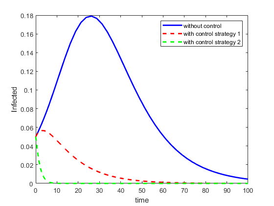
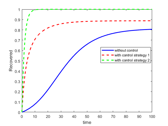
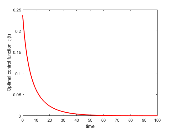
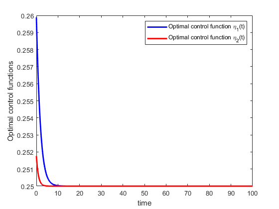
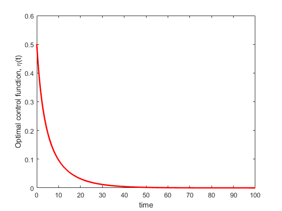
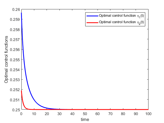
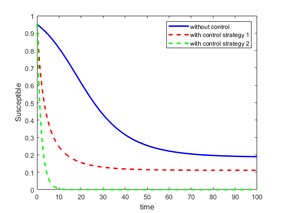
This subsection deals with numerical solutions of optimal control problems formulated in subsections 2.1 and 2.2. Analytical solution of nonlinear system of differential equations with optimal control is a very hard task in mathematical modelling. Therefore, in this study, we apply the efficient forward-backward sweep numerical scheme with fourth-order Runge-Kutta method to solve the optimality systems formulated for the two optimal control strategies. This numerical scheme has extensively been described by the authors in (Lenhart and Workman, 2007) in their mathematical modelling textbook which is concern with the applications of differential equations and optimal control theory. For our numerical simulations, we have adapted the same model parameter values ($\nu=0.2,\ \delta=0.1$) as in the work by the authors in (Rachah and Torres, 2015) and initial conditions: $s_{0}=0.95,\ i_{0}=0.05,\ r_{0}=0$. For the positive parameters in the objectives functionals, we have assumed that $D=1,\ C_{1}=1,\ C_{2}=5$ and $C_{3}=5.$ In Fig. 1, it is clear that, there is a significant decrease in the number of susceptible individuals with control strategies 1, 2 than without control. Figure 2 shows solution paths for infected individuals with control strategies 1, 2 and without control. This plot shows significant decrease in the infected individuals with control strategies 1, 2 than without control. In Fig 3, there is a rapid increase in recovered individuals with control strategies 1, 2 than without control. Figures 4 and 5 represents control functions for optimal control strategies 1 and 2 respectively.

Figure 1: Solution paths for susceptible individuals with two control strategies and without control, $\nu=0.2$,  $\delta=0.1$

Figure 2: Solution paths for Infected individuals with two control strategies and without control, $\nu=0.2$,  $\delta=0.1$

Figure 3: Solution paths for Recovered individuals with two control strategies and without control, $\nu=0.2$,  $\delta=0.1$

Figure 4: Optimal control function $\eta(t)$ for strategy 1

Figure 5: Optimal control functions $\eta_{1}(t)$ and $\eta_{2}(t)$ for strategy 2

3 SEIR Model

In this section, we introduce the basic SEIR mathematical model to describe the transmission dynamics of Ebola infection. This model also assumes constant population size with no vital dynamics(birth and death rates). The total population is divided into four different classes with $S(t),\ E(t),\ E(t)$ and $R(t)$ representing Susceptible, Exposed, Infectious and Recovered individuals respectively. Following the compartmental modeling concepts in (Hethcote, 2000), the nonlinear dynamical system describing Ebola virus disease is given by

$$\begin{cases}\displaystyle\frac{dS(t)}{dt}=\displaystyle{-\frac{\nu S(t)I(t)}{N}},\ \ \ \qquad\qquad\qquad S(0)=S_{0}\geq 0,\\ \\ \displaystyle\frac{dE(t)}{dt}=\displaystyle{\frac{\nu S(t)I(t)}{N}}-{\rho}{E(t)},\ \ \ \ \ \qquad E(0)=E_{0}\geq 0,\\ \\ \displaystyle\frac{dI(t}{dt}=\displaystyle{\rho E(t)}-{\delta}{I(t)},\ \ \qquad\qquad\qquad I(0)=I_{0}\geq 0,\\ \\ \displaystyle\frac{dR(t)}{dt}=\displaystyle{\delta I(t)},\qquad\qquad\qquad\qquad\qquad R(0)=R_{0}\geq 0.\end{cases}$$ (19)

with $S(t)+E(t)+I(t)+R(t)=N,$

where $\nu$ is the transmission rate, $\rho$ represent the infectious rate and $\delta$ is the recovery rate.

As we did in section 2, we will work with proportional quantities instead of the actual populations by scaling each state variable ($S(t),\ E(t),\ I(t),\ R(t)$) by the total population. We therefore introduce new state variables ($s(t),\ e(t),\ i(t),\ r(t)$) which are expressed in terms of the original state variables and the total population is given by

$$\begin{cases}s(t)=\frac{S(t)}{N},\\ \\ e(t)=\frac{E(t)}{N},\\ \\ i(t)=\frac{I(t)}{N},\\ \\ r(t)=\frac{R(t)}{N}.\end{cases}$$ (20)

By differentiating the scaling equation (20) with respect to time $t$ and using the unscaled model problem (19), we obtain the scaled SEIR model as follows

$$\begin{cases}\displaystyle\frac{ds(t)}{dt}=\displaystyle{-\nu s(t)i(t)},\ \qquad\qquad\qquad s(0)=s_{0}\geq 0,\\ \\ \displaystyle\frac{de(t)}{dt}=\displaystyle{\nu s(t)i(t)}-{\rho}{e(t)},\qquad\qquad e(0)=e_{0}\geq 0,\\ \\ \displaystyle\frac{di(t)}{dt}=\displaystyle{\rho e(t)}-{\delta}{i(t)},\qquad\qquad\qquad i(0)=i_{0}\geq 0,\\ \\ \displaystyle\frac{dr(r)}{dt}=\displaystyle{\delta i(t)},\ \ \ \qquad\qquad\qquad\qquad r(0)=r_{0}\geq 0.\end{cases}$$ (21)

with $s(t)+e(t)+i(t)+r(t)=1,$

where the new state variables $s(t)\,e(t),\ i(t)$ and $r(t)$ represent proportions of Susceptible, Infected and Recovered individuals respectively.

As in (Rachah and Torres, 2016), we will use this scaled SEIR model problem (21) in subsections 3.1,  3.2 and 3.3 to construct optimal control models for Ebola infection with three different control strategies.

3.1 SEIR Model with Optimal Control Strategy 1

In this subsection, we consider a controlled dynamical system for the scaled SEIR model (21), using vaccination as time dependent control function, $\eta(t)$. As we did in subsection 2.1, our main objective for this optimal control problem is that, we want to reduce the number of infected individuals and the cost of vaccination. Therefore in this control strategy, we minimize the objective functional $J(\eta)$ given by

$$J(\eta)=\int^{t_{f}}_{0}\left[i(t)+\dfrac{D}{2}\eta^{2}(t)\right]dt$$ (22)

subject to:

$$\begin{cases}\displaystyle\frac{ds(t)}{dt}=\displaystyle{-\nu s(t)i(t)-\eta(t)s(t)},\ \qquad\qquad s(0)=s_{0}\geq 0,\\ \\ \displaystyle\frac{de(t)}{dt}=\displaystyle{\nu s(t)i(t)}-{\rho}{e(t)},\qquad\qquad\qquad e(0)=e_{0}\geq 0,\\ \\ \displaystyle\frac{di(t)}{dt}=\displaystyle{\rho e(t)}-{\delta}{i(t)},\qquad\qquad\qquad\qquad i(0)=i_{0}\geq 0,\\ \\ \displaystyle\frac{dr(t)}{dt}=\displaystyle{\delta i(t)+\eta(t)s(t)},\ \ \qquad\qquad\qquad r(0)=r_{0}\geq 0.\end{cases}$$ (23)

where the control set is given by

$${\mathcal{G}}_{3}=\{\eta\mathrel{\mathop{\mathchar 58\relax}}\eta(t)\ \textrm{is lebesgue measurable},\ 0\leq\eta(t)\leq 1,\ t\in[0,t_{f}]\}$$

and the positive constant $D$ is the weight on the cost of vaccination.

The Hamiltonian function $H$ is then given as:

$$\begin{split}H&=i(t)+\dfrac{D}{2}\eta^{2}(t)\\ \\ &+\varphi_{1}\left[-\nu s(t)i(t)-\eta(t)s(t)\right]\\ \\ &+\varphi_{2}\left[\nu s(t)i(t)-\rho e(t)\right]\\ \\ &+\varphi_{3}\left[\rho e(t)-\delta i(t)\right]\\ \\ &+\varphi_{4}\left[\delta i(t)+\eta(t)s(t)\right]\end{split}$$ (24)

We then apply the Maximum Principle proposed by authors in (Pontryagin et al., 1962) to determine an optimal solution as

Given that $(w,\eta)$ is an optimal solution for a controlled dynamical system, then there exist adjoint vector function $\varphi=(\varphi_{1},\ \varphi_{2},\ \cdots\varphi_{n})$ which satisfy the following equations

$$\begin{cases}\frac{dw}{dt}={\frac{\partial H(t,w,\eta,\varphi)}{\partial\varphi}},\\ \\ 0={\frac{\partial H(t,w,\eta,\varphi)}{\partial\eta}},\\ \\ \frac{d\varphi}{dt}=-{\frac{\partial H(t,w,\eta,\varphi)}{\partial w}}.\end{cases}$$ (25)

Using the formulated Hamiltonian function (24) and equation (25), the adjoint equations and the control characterisation are presented in the following Theorem.

Theorem 3

Let ${\eta}^{*}$ be an optimal control and optimal state solutions $s^{*},e^{*},i^{*},r^{*}$ of the corresponding controlled dynamical system (22)-(23) that minimize $J(\eta)$ over ${\mathcal{G}}_{3}$. Then there exist adjoint variables $\varphi_{i}$  for $i=1,2,3,4$ satisfying

$$\begin{cases}\displaystyle\frac{d\varphi_{1}}{dt}=\displaystyle{\nu i^{*}(t)(\varphi_{1}-\varphi{2})+\eta^{*}(t)(\varphi_{1}-\varphi_{4})},\qquad\\ \\ \displaystyle\frac{d\varphi_{2}}{dt}=\displaystyle{\rho(\varphi_{2}-\varphi_{3})},\qquad\\ \\ \displaystyle\frac{d\varphi_{3}}{dt}=\displaystyle{-1+\nu s^{*}(t)(\varphi_{1}-\varphi_{2})+\delta(\varphi_{3}-\varphi_{4})},\qquad\\ \\ \displaystyle\frac{d\varphi_{4}}{dt}=\displaystyle{0}.\qquad\end{cases}$$ (26)

with transversality conditions $\varphi_{1}(t_{f})=0,\ \varphi_{2}(t_{f})=0,\ \varphi_{3}(t_{f})=0,\ \varphi_{4}(t_{f})=0$ and the control $\eta^{*}(t)$ satisfies the optimality condition.

$$\eta^{*}(t)=min\left\{max\left\{0,\dfrac{s^{*}}{D}(\varphi_{1}-\varphi_{4})\right\},1\right\}$$ (27)

3.2 SEIR Model with Optimal Control Strategy 2

In this subsection, we present a controlled dynamical system for the scaled SEIR model (21), using vaccination as time dependent control function, $\eta(t)$. Our main objective for this strategy is to reduce number of infected and exposed individuals as were as the cost of vaccination. Therefore in this control strategy, we minimize the objective functional $J(\eta)$ given by

$$J(\eta)=\int^{t_{f}}_{0}\left[K_{1}e(t)+K_{2}i(t)+\dfrac{K_{3}}{2}\eta^{2}(t)\right]dt$$ (28)

subject to:

$$\begin{cases}\displaystyle\frac{ds(t)}{dt}=\displaystyle{-\nu s(t)i(t)-\eta(t)s(t)},\ \qquad\qquad s(0)=s_{0}\geq 0,\\ \\ \displaystyle\frac{de(t)}{dt}=\displaystyle{\nu s(t)i(t)}-{\rho}{e(t)},\ \ \ \ \ \ \qquad\qquad e(0)=e_{0}\geq 0,\\ \\ \displaystyle\frac{di(t)}{dt}=\displaystyle{\rho e(t)}-{\delta}{i(t)},\qquad\qquad\qquad\qquad i(0)=i_{0}\geq 0,\\ \\ \displaystyle\frac{dr(t)}{dt}=\displaystyle{\delta i(t)+\eta(t)s(t)},\ \ \qquad\qquad\qquad r(0)=r_{0}\geq 0.\end{cases}$$ (29)

where the control set is given as:

$${\mathcal{G}}_{4}=\{\eta\mathrel{\mathop{\mathchar 58\relax}}\eta(t)\ \textrm{is lebesgue measurable},\ 0\leq\eta(t)\leq 1,\ t\in[0,t_{f}]\}$$

and the parameters $K_{1}$ and $K_{2}$ are positive constants associated with exposed individuals and infected individuals and $K_{3}$ is a positive weight constant for control function $\eta(t)$.

The Hamiltonian $H$ is given by

$$\begin{split}H&=K_{1}e(t)+K_{2}i(t)+\dfrac{K_{3}}{2}\eta^{2}(t)\\ \\ &+\varphi_{1}\left[-\nu s(t)i(t)-\eta(t)s(t)\right]\\ \\ &+\varphi_{2}\left[\nu s(t)i(t)-\rho e(t)\right]\\ \\ &+\varphi_{3}\left[\rho e(t)-\delta i(t)\right]\\ \\ &+\varphi_{4}\left[\delta i+\eta(t)s(t)\right]\end{split}$$ (30)

We then apply the Maximum Principle proposed by authors in (Pontryagin et al., 1962) to determine an optimal solution as

Assume that $(w,\eta)$ is an optimal solution for a controlled dynamical system, then there exist adjoint vector function $\varphi=(\varphi_{1},\ \varphi_{2},\ \cdots\varphi_{n})$ which satisfy the following equations

$$\begin{cases}\frac{dw}{dt}={\frac{\partial H(t,w,\eta,\varphi)}{\partial\varphi}},\\ \\ 0={\frac{\partial H(t,x,\eta,\varphi)}{\partial\eta}},\\ \\ \frac{d\varphi}{dt}=-{\frac{\partial H(t,w,\eta,\varphi)}{\partial w}}.\end{cases}$$ (31)

Using the formulated Hamiltonian function (30) and equation (31), the adjoint equations and the control characterisation are given in the following Theorem as

Theorem 4

Let ${\eta}^{*}$ be an optimal control and optimal state solutions $s^{*},e^{*},i^{*},r^{*}$ of the corresponding controlled dynamical system (28)-(29) that minimize $J(\eta)$ over ${\mathcal{G}}_{3}$. Then there exist adjoint variables $\varphi_{i}$  for $i=1,2,3,4$ satisfying

$$\begin{cases}\displaystyle\frac{d\varphi_{1}}{dt}=\displaystyle{\nu i^{*}(t)(\varphi_{1}-\varphi{2})+\eta^{*}(t)(\varphi_{1}-\varphi_{4})},\qquad\\ \\ \displaystyle\frac{d\varphi_{2}}{dt}=\displaystyle{-K_{1}+\rho(\varphi_{2}-\varphi_{3})},\qquad\\ \\ \displaystyle\frac{d\varphi_{3}}{dt}=\displaystyle{-K_{2}+\nu s^{*}(t)(\varphi_{1}-\varphi_{2})+\delta(\varphi_{3}-\varphi_{4})},\qquad\\ \\ \displaystyle\frac{d\varphi_{4}}{dt}=\displaystyle{0}.\end{cases}$$ (32)

with transversality conditions $\varphi_{1}(t_{f})=0,\ \varphi_{2}(t_{f})=0,\ \varphi_{3}(t_{f})=0,\ \varphi_{4}(t_{f})=0$ and the control function $\eta^{*}$ is given by

$$\eta^{*}(t)=min\left\{max\left\{0,\dfrac{s^{*}(t)}{K_{3}}(\varphi_{1}-\varphi_{4})\right\},1\right\}$$ (33)

3.3 SEIR Model with Optimal Control Strategy 3

In this subsection, we present a controlled dynamical problem by incorporating treatment control, $\eta_{1}(t)$ and educational campaign control, $\eta_{2}(t)$ into the SEIR model (3). As we presented in subsection 2.2, our main aim for this controlled problem is to minimize the number of infected individuals, the cost of educational campaigns and treatment. Therefore in this control strategy, we minimise the objective functional given by

$$J(\eta_{1},\eta_{2})=\int^{t_{f}}_{0}\left[D_{1}i(t)]+\dfrac{D_{2}}{2}\eta^{2}_{1}(t)+\dfrac{D_{3}}{2}\eta^{2}_{2}(t)\right]dt$$ (34)

Subject to:

$$\begin{cases}\displaystyle\frac{ds(t)}{dt}=\displaystyle{-\nu s(t)i(t)-\eta_{2}(t)s(t)},\ \ \ \ \qquad\qquad\qquad s(0)=s_{0}\geq 0,\\ \\ \displaystyle\frac{de(t)}{dt}=\displaystyle{\nu s(t)i(t)}-{\rho}{e(t)},\ \ \ \ \ \ \qquad\qquad\qquad\qquad e(0)=e_{0}\geq 0,\\ \\ \displaystyle\frac{di(t)}{dt}=\displaystyle{\rho e(t)}-{\delta}{i(t)}-\eta_{1}(t)i(t),\ \ \qquad\qquad\qquad i(0)=i_{0}\geq 0,\\ \\ \displaystyle\frac{dr(t)}{dt}=\displaystyle{\delta i(t)+\eta_{1}(t)i(t)+\eta_{2}(t)s(t)},\ \ \ \ \qquad\qquad r(0)=r_{0}\geq 0.\end{cases}$$ (35)

where the control set is given as:

$${\mathcal{G}}_{5}=\{(\eta_{1},\eta_{2})\mathrel{\mathop{\mathchar 58\relax}}\eta_{i}(t)\ \textrm{is lebesgue measurable},\ 0\leq\eta_{i}(t)\leq 1,\ t\in[0,t_{f}]\ \textrm{for}\ i=1,2\}$$

where $D_{1}$ is the weight constant on infected individuals and $D_{2}$ and $D_{3}$ are also positive weight parameters associated with controls $\eta_{1}(t)$ and $\eta_{2}(t)$ respectively.

The Hamiltonian function $H$ is given as

$$\begin{split}H&=D_{1}i(t)]+\dfrac{D_{2}}{2}\eta^{2}_{1}(t)+\dfrac{D_{3}}{2}\eta^{2}_{2}(t)\\ \\ &+\varphi_{1}\left[-\nu s(t)i(t)-\eta_{2}(t)s(t)\right]\\ \\ &+\varphi_{2}\left[\nu s(t)i(t)-\rho e(t)\right]\\ \\ &+\varphi_{3}\left[\rho e(t)-\delta i(t)-\eta_{1}(t)i(t)\right]\\ \\ &+\varphi_{4}\left[\delta i(t)+\eta_{1}(t)i(t)+\eta_{2}(t)s(t)\right]\end{split}$$ (36)

We then apply the Maximum Principle proposed by authors in (Pontryagin et al., 1962) to determine an optimal solution as

Assume that $(w,\eta)$ is an optimal solution for a controlled dynamical system, then there exist adjoint vector function $\varphi=(\varphi_{1},\ \varphi_{2},\ \cdots\varphi_{n})$ which satisfy the following equations

$$\begin{cases}\frac{dw}{dt}={\frac{\partial H(t,w,\eta,\varphi)}{\partial\varphi}},\\ \\ 0={\frac{\partial H(t,w,\eta,\varphi)}{\partial\eta}},\\ \\ \frac{d\varphi}{dt}=-{\frac{\partial H(t,w,\eta,\varphi)}{\partial w}}.\end{cases}$$ (37)

Using the formulated Hamiltonian function (36) and equation (37), the adjoint equations and the control characterisation are presented in the following Theorem.

Theorem 5

Let $\eta^{*}_{1}$ and $\eta^{*}_{2}$ be optimal control pair and optimal state solutions $s^{*},e^{*},i^{*},r^{*}$ of the corresponding controlled dynamical system (34)-(35) that minimize $J(\eta_{1},\eta_{2})$ over ${\mathcal{G}}_{5}$. Then there exist adjoint variables $\varphi_{i}$  for $i=1,2,3,4$ satisfying

$$\begin{cases}\displaystyle\frac{d\varphi_{1}}{dt}=\displaystyle{\nu i^{*}(t)(\varphi_{1}-\varphi_{2})+\eta^{*}_{2}(t)(\varphi_{1}-\varphi_{4})},\qquad\\ \\ \displaystyle\frac{d\varphi_{2}}{dt}=\displaystyle{\rho(\varphi_{2}-\varphi_{3})},\qquad\\ \\ \displaystyle\frac{d\varphi_{3}}{dt}=\displaystyle{-D_{1}+\nu s^{*}(t)(\varphi_{1}-\varphi_{2})+\delta(\varphi_{3}-\varphi_{4})+\eta^{*}_{1}(t)(\varphi_{3}-\varphi_{4})},\qquad\\ \\ \displaystyle\frac{d\varphi_{4}}{dt}=\displaystyle{0}.\qquad\end{cases}$$ (38)

with transversality conditions $\varphi_{1}(t_{f})=0,\ \varphi_{2}(t_{f})=0,\ \varphi_{3}(t_{f})=0,\ \varphi_{4}(t_{f})=0$

and the control pair $\eta^{*}_{1}$ and $\eta^{*}_{2}$ satisfies the optimality condition.

$$\begin{cases}\displaystyle\eta^{*}_{1}(t)=min\left\{max\left\{0,\dfrac{i^{*}(t)}{D_{2}}(\varphi_{3}-\varphi_{4})\right\},1\right\}\\ \\ \displaystyle\eta^{*}_{2}(t)=min\left\{max\left\{0,\dfrac{s^{*}(t)}{D_{3}}(\varphi_{1}-\varphi_{4})\right\},1\right\}\end{cases}$$ (39)

3.4 Numerical Simulations and Discussions

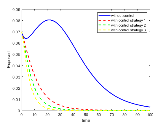
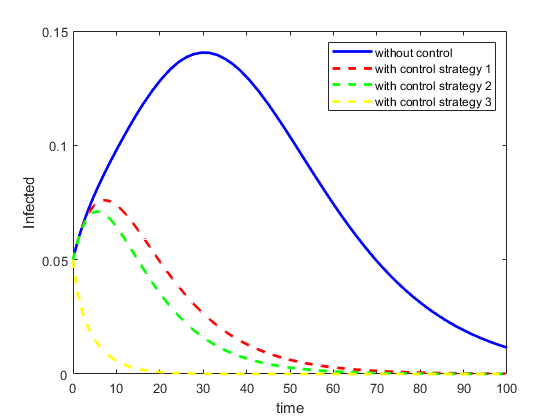
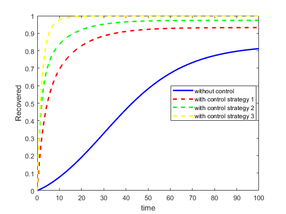
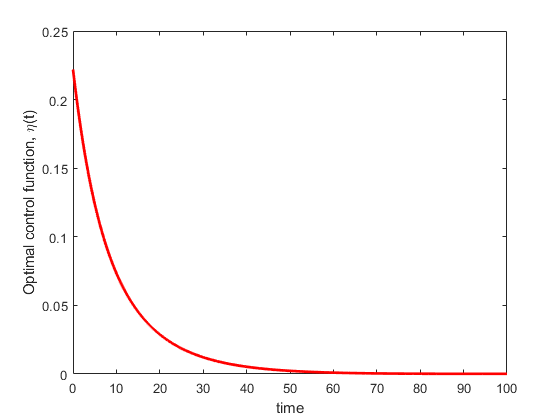
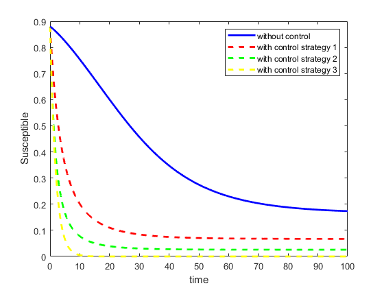
As we did in subsection 2.3, we have used the forward-backward sweep numerical scheme with fourth order Runge-Kutta method to solve the optimality systems formulated for the three optimal control strategies. For our numerical simulations, we have adapted the same model parameter values ($\nu=0.2,\ \delta=0.1,\ \rho=0.1887$) as in the work by the authors in (Rachah and Torres, 2016) with initial conditions: $s_{0}=0.88,\ e_{0}=0.07,\ i_{0}=0.05,\ r_{0}=0$. We have assumed $D=5,\ K_{1}=1,\ K_{2}=5,\ K_{3}=5,\ D_{1}=1,\ D_{2}=5$ and $D_{3}=5$. Figure 6 shows solution paths for susceptible individuals with control strategies $1,2,3$ and without control. It is clear from the plot that, there is a significant decrease in the number of susceptible individuals with control strategies than without control. In Fig. 7, there is a rapid decrease in exposed individuals with control strategies $1,2,3$ than without control. A similar effect can be observed in Fig. 8 for the infected individuals. In Fig. 9, there is a rapid increase in recovered individuals with control strategies $1,2,3$ than without control. Figures 10,  11, and 12 represents optimal control functions for strategies 1, 2 and 3 respectively.

Figure 6: Solution path for Susceptible individuals with three control strategies and without control, $\nu=0.2$, $\rho=0.1887$,  $\delta=0.1$

Figure 7: Solution paths for Exposed individuals with three control strategies and without control, $\nu=0.2$, $\rho=0.1887$,  $\delta=0.1$

Figure 8: Solution paths for Infected individuals with three control strategies and without control, $\nu=0.2$, $\rho=0.1887$,  $\delta=0.1$

Figure 9: Solution paths for Recovered individuals with three control strategies and without control, $\nu=0.2$, $\rho=0.1887$,  $\delta=0.1$

Figure 10: Optimal control function $\eta(t)$ for strategy 1

Figure 11: Optimal control functions $\eta(t)$ for strategy 2

Figure 12: Optimal control functions $\eta_{1}(t)$ and $\eta_{2}(t)$ for strategy 3

4 Conclusion

In this paper, we have studied epidemiological models for Ebola virus disease using nonlinear system of ordinary differential equation and optimal control theory. We have used indirect methods in optimal control to study existing mathematical models proposed by the authors in (Rachah and Torres, 2015, 2016). Using the Pontryagin’s maximum principle and Hamiltonian function, we have derived adjoint equations and optimality system for the various optimal control strategies. From the simulations results, we observed that, SIR model with optimal control strategies shows significant decrease in the proportions of infected and susceptible individuals and a rapid increase in the recovered individuals compared to SIR model without control. A similar effect was observed in the SEIR model with control strategies where there was a significant decrease in Susceptible, Exposed and Infected individuals and a rapid increase in the Recovered individuals. Our numerical results are similar to the once generated by the authors in (Rachah and Torres, 2015, 2016) who applied direct methods in optimal control for their mathematical models. Therefore, following the numerical results, we can conclude that, effective educational campaigns and vaccination of susceptible individuals as were as effective treatments of infected individuals can help reduced the disease transmission. In this work, we have also analytically and numerical studied one additional optimal control strategy for the SIR epidemic model.

References

• Agusto et al. (2015) F. B . Agusto, M. I. Teboh-Ewungkem, and A. B Gumel. Mathematical assessment of the effect of traditional beliefs and customs on the transmission dynamics of the 2014 ebola outbreaks. BMC medicine, 13(1):96, 2015.
• Ahmad et al. (2016) M. D. Ahmad, M. Usman, A. Khan, and M. Imran. Optimal control analysis of ebola disease with control strategies of quarantine and vaccination. Infectious diseases of poverty, 5(1):72, 2016.
• Althaus (2014) C. L. Althaus. Estimating the reproduction number of ebola virus (ebov) during the 2014 outbreak in west africa. PLoS currents, 6, 2014.
• Area et al. (2018) I. Area, F. Ndaïrou, J. J Nieto, C. J. Silva, and D. F. M. Torres. Ebola model and optimal control with vaccination constraints. Journal of Industrial and Management Optimization, 14(2):427–466, 2018.
• Atangana and Goufo (2014) A. Atangana and E. F. D. Goufo. On the mathematical analysis of ebola hemorrhagic fever: deathly infection disease in west african countries. BioMed research international, 2014, Article ID 261383:7 pages, 2014.
• Berge et al. (2017) T. Berge, J. M-S. Lubuma, G. M Moremedi, N. Morris, and R. Kondera-Shava. A simple mathematical model for ebola in africa. Journal of biological dynamics, 11(1):42–74, 2017.
• Bonyah et al. (2016) E. Bonyah, K. Badu, and S. K. Asiedu-Addo. Optimal control application to an ebola model. Asian Pacific Journal of Tropical Biomedicine, 6(4):283–289, 2016.
• Bonyah et al. (2017) E. Bonyah, M. A. Khan, K. O. Okosun, and S. Islam. A theoretical model for zika virus transmission. PloS one, 12(10):e0185540, 2017.
• Bonyah et al. (2019) E. Bonyah, M. A. Khan, K. O. Okosun, and J. F. Gómez-Aguilar. On the co‐infection of dengue fever and zika virus. Optim Control Appl Meth, pages 1–28, 2019.
• Chowell and Nishiura (2014) G. Chowell and H. Nishiura. Transmission dynamics and control of ebola virus disease (evd): a review. BMC medicine, 12(1):196, 2014.
• Chowell et al. (2004) G. Chowell, N. W. Hengartner, C. Castillo-Chavez, P. W. Fenimore, and J. M. Hyman. The basic reproductive number of ebola and the effects of public health measures: the cases of congo and uganda. Journal of theoretical biology, 229(1):119–126, 2004.
• Dénes and Gumel (2019) A. Dénes and A. B. Gumel. Modeling the impact of quarantine during an outbreak of ebola virus disease. Infectious Disease Modelling, 4:12–27, 2019.
• Diaz et al. (2018) P. Diaz, P. Constantine, K. Kalmbach, E. Jones, and S. Pankavich. A modified seir model for the spread of ebola in western africa and metrics for resource allocation. Applied Mathematics and Computation, 324:141–155, 2018.
• Dong et al. (2015) F. Dong, D. Xu, Z. Wang, and M. Dong. Evaluation of ebola spreading in west africa and decision of optimal medicine delivery strategies based on mathematical models. Infection, Genetics and Evolution, 36:35–40, 2015.
• Goufo et al. (2016) E. F. D. Goufo, M. K. Pene, and S. Mugisha. Stability analysis of epidemic models of ebola hemorrhagic fever with non-linear transmission. Journal of Nonlinear Sciences & Applications (JNSA), 9(6), 2016.
• Grigorieva et al. (2017) E. V. Grigorieva, P. B. Deignan, and E. N Khailov. Optimal control problem for a seir type model of ebola epidemics. Revista de Matemática: Teoría y Aplicaciones, 24(1):79–96, 2017.
• Hethcote (2000) H. W. Hethcote. The mathematics of infectious diseases. SIAM review, 42(4):599–653, 2000.
• Jiang et al. (2017) S. Jiang, K. Wang, C. Li, G. Hong, X. Zhang, M. Shan, H. Li, and J. Wang. Mathematical models for devising the optimal ebola virus disease eradication. Journal of translational medicine, 15(1):124, 2017.
• Khan et al. (2015) A. Khan, M. Naveed, M. Dur-e-Ahmad, and M. Imran. Estimating the basic reproductive ratio for the ebola outbreak in liberia and sierra leone. Infectious diseases of poverty, 4(1):13, 2015.
• Khan et al. (2019) M. A. Khan, S. W. Shah, S. Ullah, and J. F. Gómez-Aguilar. A dynamical model of asymptomatic carrier zika virus with optimal control strategies. Nonlinear Analysis: Real World Applications, 50:144–170, 2019.
• Lenhart and Workman (2007) S. Lenhart and J. T. Workman. Optimal control applied to biological models. Chapman and Hall/CRC, 2007.
• Luo et al. (2019) D. Luo, R. Zheng, D. Wang, X. Zhang, Y. Yin, K. Wang, and W. Wang. Effect of sexual transmission on the west africa ebola outbreak in 2014: a mathematical modelling study. Scientific reports, 9, 2019.
• Miyaoka et al. (2019) T. Y. Miyaoka, S. Lenhart, and J. C. A. Meyer. Optimal control of vaccination ina vector-borne reaction-diffusion model applied to zika virus. Journal of Mathematical Biology, pages 1–28, 2019.
• Ndanguza et al. (2017) D. Ndanguza, I. S. Mbalawata, H. Haario, and J. M. Tchuenche. Analysis of bias in an ebola epidemic model by extended kalman filter approach. Mathematics and Computers in Simulation, 142:113–129, 2017.
• Ngwa and Teboh-Ewungkem (2016) G. A. Ngwa and M. I. Teboh-Ewungkem. A mathematical model with quarantine states for the dynamics of ebola virus disease in human populations. Computational and mathematical methods in medicine, vol. 2016, Article ID 9352725:29 pages, 2016.
• Pontryagin et al. (1962) L. S. Pontryagin, V.G. Boltyanskii, R. V. Gamkrelidze, and E. F. Mishchenko. The mathematical theory of optimal processes. New York, John Wiley & Sons, 1962.
• Rachah and Torres (2015) A. Rachah and D. F. M. Torres. Mathematical modelling, simulation, and optimal control of the 2014 ebola outbreak in west africa. Discrete Dynamics in Nature and Society, vol. 2015, Article ID 842792:9 pages, 2015.
• Rachah and Torres (2016) A. Rachah and D. F. M. Torres. Dynamics and optimal control of ebola transmission. Mathematics in Computer Science, 10(3):331–342, 2016.
• Sharomi and Malik (2017) O. Sharomi and T. Malik. Optimal control in epidemiology. Annals of Operations Research, 251(1-2):55–71, 2017.
• Tulu et al. (2017) T. W. Tulu, B. Tian, and Z. Wu. Mathematical modeling, analysis and markov chain monte carlo simulation of ebola epidemics. Results in physics, 7:962–968, 2017.
• Weitz and Dushoff (2015) J. S. Weitz and J. Dushoff. Modeling post-death transmission of ebola: challenges for inference and opportunities for control. Scientific reports, 5:8751, 2015.
• WHO (2019) WHO. Ebola virus disease, https://www.who.int/news-room/fact-sheets/detail/ebola-virus-disease, 2019.
• Xia et al. (2015) Zhi-Qiang Xia, Shi-Fu Wang, Shen-Long Li, Liu-Yu Huang, Wen-Yi Zhang, Gui-Quan Sun, Zhong-Tao Gai, and Zhen Jin. Modeling the transmission dynamics of ebola virus disease in liberia. Scientific reports, 5:13857, 2015.
• Zakary et al. (2017) O. Zakary, M. Rachik, and I. Elmouki. A multi-regional epidemic model for controlling the spread of ebola: awareness, treatment, and travel-blocking optimal control approaches. Mathematical Methods in the Applied Sciences, 40(4):1265–1279, 2017.