Steady state cyclic behaviour of a half-plane contact in partial slip subject to varying normal load, moment, shear load, and moderate differential bulk tension

Abstract

A new solution for a general half-plane contact in the steady state is presented. The contacting bodies are subject to a set of constant loads - normal force, shear force and bulk tension parallel with the interface - together with an oscillatory set of the same quantities. Partial slip conditions are expected to ensue for a range of these quantities. In addition, the line of action of the normal load component does not necessarily need to pass the centre-line of the contact, thereby introducing a moment and asymmetry in the contact extent. This advancement enables a mapping to be formalised between the normal and tangential problem. An exact and easy to apply recipe is defined.

Keywords: Contact mechanics; Half-plane theory; Partial slip; Varying normal and shear loads; Moment; Moderate bulk tension, Mapping

1 Introduction

We have recently published a partial-slip contact solution [1] for the half-plane problem in which a contact is formed by the application of a normal load $P$, and a shear force $Q$ is also gradually exerted while differential tensions $\sigma$ arise in the surfaces of the contacting bodies. These quantities then vary periodically with time and in phase with each other, so that the trajectory in ($P$, $Q$, $\sigma$) space consists of a line from the origin to some point in the steady state followed by reciprocating behaviour along a straight line between two points whose separation from the mid-point ($P_{0}$, $Q_{0}$, $\sigma_{0}$) is ($\pm\Delta P/2$, $\Delta Q/2$, $\Delta\sigma/2$). This procedure is very useful for analysing a range of practical problems, such as the gas turbine fan-blade dovetail root contact, and is straightforward to implement, but it lacks one feature present in the prototype. In the dovetail problem, as in other contact problems of this class, the line of action of the normal load does not necessarily pass through the centre-line of the contact, and it generally varies with time. Thus, a moment, $M$, develops and the contact extent becomes asymmetric.

The purpose of this sequel is to remedy that deficiency, though at the expense of greater algebraic effort. Following the same pattern of representation as used before, the mean moment developed will be denoted by $M_{0}$ and its range by $\Delta M$. The oscillatory behaviour is in phase with the other changes experienced by the contact and, as before, we neglect the transient problem and argue that, because the prototype experiences many tens of thousands of oscillatory cycles for each major change of load, it is the steady state behaviour which is of most practical importance. We further argue that, when once the permanent stick zone is known, together with the evolution of the contact patch, the most important information needed for a fretting-fatigue analysis is effectively established. We then know the maximum extents of slip, attained just before the points of load reversal are reached, and other things such as the slip displacement can be evaluated afterwards.

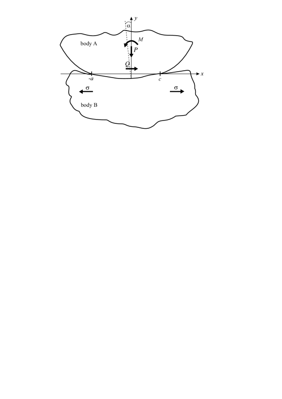
Figure 1: Generic half-plane contact subject to normal load, moment, shear load and bulk tension.

Figure 1 shows a generic half-plane contact, subject to normal load, moment, shear load, and bulk tension loading, for reference. Note, in particular, the sense of a positive applied moment which will be needed in some of the results to be found.

The majority of partial slip solutions known in the literature employ a method in which the shear traction distribution is viewed as the sum of that due to sliding, superimposed with a corrective term. Hertz was the first to find the solution to the normal contact problem where the contacting bodies have second order (strictly parabolic but usually interpreted as circular arc) profiles [2], so it is natural that the first partial slip contact solutions were all associated with the same type of geometry. The first solution, for a subsequently monotonically increasing shear force, was found by Cattaneo [3], and, apparently unaware of this solution, Mindlin [4] developed the same solution and went on to look at unloading and reloading problems [5], [6]. These were the only significant solutions for some time, and then Nowell and Hills [7] looked at what happened when a bulk tension was simultaneously exerted in one body as the shear force was gradually increased. The next breakthrough came with the near simultaneous discovery by Jäger [8] and Ciavarella [9] that, just as the ‘corrective’ shear traction was a scaled form of the sliding shear traction for the Hertz case, the same geometric similarity applies whatever the form of the contact. Major progress in solving problems involving a varying normal and shear load, and where the intention was to track out the full behaviour as a function of time, was made in [10]. But this calculation was restricted to $P$-$Q$ problems.

In the analysis which follows it is assumed that the bodies are made from the same material (or more precisely that Dundurs’ second constant vanishes) [11]. The only restriction on the profile geometry is that it should define an incomplete contact capable of supporting a moment, regardless of whether the geometry itself is unsymmetrical or symmetrical. When an external moment is applied, even a symmetrical ‘indenter’ gives rise to an unsymmetrical contact, and this an important extra feature of the solution absent from this paper’s precursor.

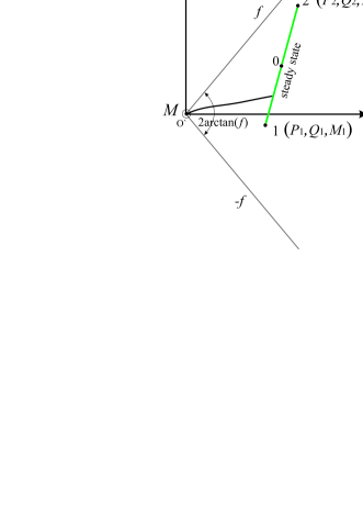
Figure 2: Two (a) and three-dimensional (b) illustration of a load space for a $P$-$Q$-$M$ problem.

It is difficult to visualise the problem in an abstract four-dimensional space. Therefore, it is valuable, first, to visualise the history of loading in the two-dimensional load space depicted in Figure 2 (a), ignoring the bulk tension. The initial loading takes us to a point coinciding with the steady state trajectory and the steady-state fluctuations are of range ($\Delta P$, $\Delta Q$, $\Delta M$) so that the loading trajectory moves between points ($P_{1}$, $Q_{1}$, $M_{1}$) and ($P_{2}$, $Q_{2}$, $M_{2}$) passing the mid-point ($P_{0}$, $Q_{0}$, $M_{0}$) every half-cycle. The most likely points to slip are the contact edges, and the contact advances at both edges while going from load point 1 to load point 2.

Note that, while both normal load and moment ($P$, $M$) affect the contact size, and all four quantities ($P$, $Q$, $M$, $\sigma$) affect the propensity of the contact to slip, only ($P$, $Q$) affect its tendency to slide. In Figure 2 (b) we sketch the loading trajectory in a three-dimensional load space from a rotated perspective, and note that the planes implying sliding have a gradient $\pm f$, where $f$ is the coefficient of friction, with respect to the $P$-axis. We will assume that the mean and oscillatory load components are such that the loading trajectory remains, at all times, within the partial slip ‘wedge’ and note that the solution potentially depends on eight quantities ($P_{0}$, $Q_{0}$, $M_{0}$, $\sigma_{0}$, $\Delta P$, $\Delta Q$, $\Delta M$, $\Delta\sigma$), together, of course, with the contact profile, material, and the coefficient of friction.

1.1 No slip condition

Before proceeding to the partial slip solution, we start by establishing the condition for permanent stick, so that no points on the contact suffer slip at any time. The sign convention shown in Figure 1 is important in what follows. Suppose that we have a contact whose instantaneous half-width is $d$, and we make a small change, $\Delta P$, in normal load together with a small change in moment, $\Delta M$. The corresponding change in contact pressure is given by [12]

$$\Delta p(x)=\frac{\Delta P}{\pi\sqrt{d^{2}-x^{2}}}+\frac{2\Delta Mx}{\pi d^{2}\sqrt{d^{2}-x^{2}}}.$$ (1)

If at the same time there are small changes in shear force, $\Delta Q,$ and differential bulk tension, $\Delta\sigma_{0},$ where the latter is, here, exerted only in body B, Figure 1, the change in shear traction, $\Delta q(x),$ generated is given by

$$\Delta q(x)=\frac{\Delta Q}{\pi\sqrt{d^{2}-x^{2}}}+\frac{\Delta\sigma x}{4\sqrt{d^{2}-x^{2}}}.$$ (2)

So, as the most likely points to slip are the contact edges the condition for no slip if $\Delta P>0$ is

$$\left(\frac{\Delta Q}{\Delta P}\pm\frac{\pi}{4}\frac{d\Delta\sigma}{\Delta P}\right)\left/\left(1\mp\frac{2\Delta M}{d\Delta P}\right)\right.<f,$$ (3)

where we choose the upper sign when considering the left hand side (LHS) of the contact and the lower sign when considering the right hand side (RHS) of the contact. The necessary condition for no slip is that the inequality holds at both sides of the contact. If this is the case it follows immediately that, when the loads are reversed and we are re-tracing our steps on the loading trajectory, full stick will continue to be maintained, that is the contact will never slip, at any point. Conversely, if the unloading trajectory deviates from loading one, there will be some slip.

2 Steady state slip behaviour

In this sequel [1] we shall continue to assume that the amount of bulk tension arising is small so that it is insufficient to reverse the direction of slip at either end of the contact.

The slip direction is reversed at each edge when going from point 1 to point 2 of the loading cycle compared with going from 2 to 1, and the slip zones attain their maximum extent just before the end points of the loading trajectory are reached.

2.1 Normal loading

Consider, first, the normal loading problem. At any given point in the loading cycle, the relative slope of the half-plane surfaces, $\mathrm{d}v/\mathrm{d}x$, is given by

$$\frac{\mathrm{d}v}{\mathrm{d}x}=-\frac{A}{\pi}\int_{-a}^{c}\frac{p(\xi)\,\mathrm{d}\xi}{\xi-x},$$ (4)

where the contact region is defined as $-a<x<c$ as shown in Figure 1, and the solution to be developed is mathematically exact only if the materials considered are elastically similar, having the property $E_{A},\nu_{A}=E_{B},\nu_{B}$, where

$$A=4\left(\frac{(1-\nu^{2})}{E}\right)$$

is the material compliance, $E$ being the Young’s modulus and $\nu$ Poisson’s ratio of the bodies (A, B), and plane-strain obtains. If the contacting bodies have a relative surface normal profile, $g(x)$, and one of the bodies is tilted through some small angle, $\alpha$, which varies with the applied moment, the integral equation relating the pressure to the profile is

$$\frac{\mathrm{d}g}{\mathrm{d}x}+\alpha=\frac{\mathrm{d}v}{\mathrm{d}x}=-\frac{A}{\pi}\int_{-a}^{c}\frac{p(\xi)\,\mathrm{d}\xi}{\xi-x},\text{ }-a<x<c.$$ (5)

Normal and rotational equilibrium are imposed by setting

$$P =\int_{-a}^{c}p(x)\,\mathrm{d}x,$$ (6)

$$M =\int_{-a}^{c}p(x)\,x\,\mathrm{d}x.$$ (7)

In the physical problem, the inputs are the profile, $\mathrm{d}g/\mathrm{d}x$, together with the loads $P$, $M$, and the outputs are the contact coordinates, $\left[-a,\quad c\right]$, and the angle of tilt, $\alpha$.

2.1.1 Solution

The solution of equation (5) is

$$p(x)=\frac{w(x,a,c)}{\pi A}\int_{-a}^{c}\frac{\left(g^{\prime}(\xi)+\alpha\right)\mathrm{d}\xi}{w(\xi,a,c)(\xi-x)}\;,\text{ }-a\leq x\leq c$$ (8)

[11], where $w(x,a,c)=\sqrt{(x+a)(c-x)}$. Equation (8) is subject to the consistency condition

$$\int_{-a}^{c}\frac{\left(g^{\prime}(\xi)+\alpha\right)\mathrm{d}\xi}{w(\xi,a,c)}=0\;,$$ (9)

and using the identity $\int_{-a}^{c}\frac{\mathrm{d}\xi}{w(\xi,a,c)}=\pi$, we conclude that

$$\int_{-a}^{c}\frac{g^{\prime}(\xi)}{w(\xi,a,c)}\mathrm{d}\xi=-\pi\alpha\;.$$ (10)

Further, the identity

$$\int_{-a}^{c}\frac{\mathrm{d}\xi}{w(\xi,a,c)(\xi-x)}=0,\text{ }-a\leq x\leq c$$ (11)

shows that the angle of tilt, $\alpha$, does not explicitly affect the general form of the inverted integral equation which is given by

$$p(x)=\frac{w(x,a,c)}{\pi A}\int_{-a}^{c}\frac{g^{\prime}(\xi)\mathrm{d}\xi}{w(\xi,a,c)(\xi-x)}\;,\text{ }-a\leq x\leq c\;,$$ (12)

but merely has an influence on the integration limits, [$-a,\quad c$].

2.2 Tangential loading

We turn now to tangential loading in the steady periodic state. During each half-cycle, the contact starts in a state of complete stick and slip zones grow on each side. We restrict attention to cases in which the direction of slip is the same at either end of the contact during each half-cycle, as shown in Figure 3, which represents the extent of the stick and slip zones just before each load reversal. The stick zone reaches its minimum extent at these points, and this defines the permanent stick zone $\left[-m,\quad n\right]$. Note that $-a_{1}<-m$ and $n<c_{1}$, where $a_{1}$ and $c_{1}$ are the contact coordinates at the point of the loading cycle at which the normal load $P$ is a minimum. Notice also that the stick zones just before each load reversal must be of the same extent, in order for there to be continuity of material over several cycles – it would not be possible for material to slip out but not to slip back, in the steady state, over any part of the contact.

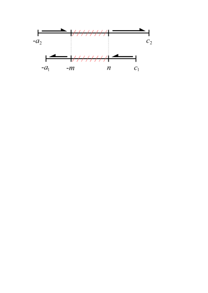
Figure 3: Contact as the ends of loading cycle are approached, including a permanent stick zone.

For load point 1 $(P_{1},Q_{1},M_{1},\sigma_{1})$ we write the relative surface strain parallel with the surface, $\Delta\varepsilon_{xx,1}$, as the sum of the effect of the sliding shear traction $-fp_{1}(x)$ over the whole contact $\left[-a_{1},\quad c_{1}\right]$ and a corrective term $q_{1}^{*}(x)$, at present unknown, over the stick region $\left[-m,\quad n\right]$. Thus,

$$\Delta\varepsilon_{xx,1}=-\frac{A}{\pi}\int_{-a_{1}}^{c_{1}}\frac{fp_{1}(\xi)\mathrm{d}\xi}{\xi-x}+\frac{A}{\pi}\int_{-m}^{n}\frac{q_{1}^{\ast}(\xi)\mathrm{d}\xi}{\xi-x}+\frac{A}{4}\sigma_{1}\;.$$ (13)

A similar expression can be written for load point 2 $(P_{2},Q_{2},M_{2},\sigma_{2})$, except that the sign of the sliding shear traction is reversed, so as to give the correct sign of shear traction in the end slip regions. We obtain

$$\Delta\varepsilon_{xx,2}=\frac{A}{\pi}\int_{-a_{2}}^{c_{2}}\frac{fp_{2}(\xi)\mathrm{d}\xi}{\xi-x}+\frac{A}{\pi}\int_{-m}^{n}\frac{q_{2}^{\ast}(\xi)\mathrm{d}\xi}{\xi-x}+\frac{A}{4}\sigma_{2}\;.$$ (14)

In the permanent stick region, the locked in difference between the surface strains must remain unchanged, i.e.

$$\Delta\varepsilon_{xx,1}=\Delta\varepsilon_{xx,2}\,\,,\text{ }-m<x<n$$ (15)

and hence, using equations (13) and (14),

$$-\frac{A}{\pi}\int_{-a_{1}}^{c_{1}}\frac{fp_{1}(\xi)\mathrm{d}\xi}{\xi-x}-\frac{A}{\pi}\int_{-a_{2}}^{c_{2}}\frac{fp_{2}(\xi)\mathrm{d}\xi}{\xi-x}-\frac{A}{4}(\sigma_{2}-\sigma_{1})=\frac{A}{\pi}\int_{-m}^{n}\frac{\left[q_{2}^{\ast}-q_{1}^{\ast}\right]\mathrm{d}\xi}{\xi-x}\;,\text{ }-m<x<n\;.$$ (16)

Since $-a_{2}<-a_{1}<-m<x<n<c_{1}<c_{2},$ we may make use of the relations from the normal contact solution, equation (5), to rewrite this equation in the form

$$\frac{2f}{A}\frac{\mathrm{d}g}{\mathrm{d}x}+\frac{2f}{A}\alpha_{0}-\frac{\Delta\sigma}{4}=\frac{1}{\pi}\int_{-m}^{n}\frac{\left[q_{2}^{\ast}-q_{1}^{\ast}\right](\xi)\mathrm{d}\xi}{\xi-x},\text{ }-m<x<n,$$ (17)

where

$$\alpha_{0}=\frac{\alpha_{1}+\alpha_{2}}{2}\rule{14.22636pt}{0.0pt}\mbox{and}\rule{14.22636pt}{0.0pt}\Delta\sigma=\sigma_{1}-\sigma_{2}$$

are respectively the average angle of tilt and the range of differential bulk tension between the two load points. It is worth noting that the LHS of equation (17) has just two terms; one is defined by the profile of the contacting bodies (as appears in the normal load problem), and the other is a constant.

2.2.1 Tangential equilibrium

We denote the resultant corrective shear forces by

$$Q_{i}^{\ast}=\int q_{i}^{\ast}(x)\mathrm{d}x\;;\;\;\;i=1,2\;,$$ (18)

so that we may now impose tangential equilibrium by setting

$$Q_{1}=-fP_{1}+Q_{1}^{\ast}\;;\;\;\;Q_{2}=fP_{2}+Q_{2}^{\ast}\;.$$ (19)

The range of shear force, $\Delta Q$, is given by

$$\Delta Q=Q_{2}-Q_{1}=2fP_{0}+\Delta Q^{\ast},$$ (20)

where

$$P_{0}=\frac{P_{1}+P_{2}}{2}$$

is the mean normal load and

$$\Delta Q^{\ast}=\int_{-m}^{n}[q_{2}^{\ast}-q_{1}^{\ast}](x)\mathrm{d}x\;.$$ (21)

2.2.2 Solution

The solution of the tangential problem can be facilitated by exploiting significant parallels with the normal contact problem of Section 2.1. For example, the inversion of equation (17), bounded at both ends, is given by

$$[q_{2}^{\ast}-q_{1}^{\ast}](x)=-\frac{w(x,m,n)}{\pi}\int_{-m}^{n}\left(\frac{2f}{A}g^{\prime}(\xi)+\frac{2f}{A}\alpha_{0}-\frac{\Delta\sigma}{4}\right)\frac{\mathrm{d}\xi}{w(\xi,m,n)(\xi-x)}$$ (22)

[11], and arguments exactly parallel to those in Section 2.1.1 lead to the results

$$\int_{-m}^{n}\frac{g^{\prime}(\xi)\mathrm{d}\xi}{w(\xi,m,n)}=-\pi\alpha_{0}+\frac{A\pi\Delta\sigma}{8f}\;,$$ (23)

and

$$[q_{2}^{\ast}-q_{1}^{\ast}](x)=-\frac{2fw(x,m,n)}{\pi A}\int_{-m}^{n}\frac{g^{\prime}(\xi)\mathrm{d}\xi}{w(\xi,m,n)(\xi-x)}\;,\text{ }-m\leq x\leq n\;.$$ (24)

This shows that the corrective shear traction is geometrically of the same form as the contact pressure distribution, but associated with a particular normal load and moment which will not be the same as those actually present on the contact.

2.3 Mapping between the normal and tangential problems

The parallels between the normal and tangential problems identified in Section 2.2.2 can be formalized by defining the mapping

$$[-a,c] \rightarrow [-m,n]$$

$$p(x) \rightarrow -\frac{1}{2f}\,[q_{2}^{*}-q_{1}^{*}](x)$$

$$P \rightarrow P_{0}-\frac{\Delta Q}{2f}$$ (25)

$$\alpha \rightarrow \alpha_{0}-\frac{A\Delta\sigma}{8f}$$

If the normal contact problem for an indenter of given profile $g^{\prime}(x)$ can be solved, meaning that we can determine closed form expressions for the contact coordinates $[-a,c]$ and the pressure distribution $p(x)$ for arbitrary values of $P$ and $\alpha$, the solution to the steady-state tangential problem can then be found readily mutatis mutandis, using the above mapping. In many cases, the normal problem will be defined in terms of the forces $P_{i}$ and the moments $M_{i}$, $i=1,2$, in which case a preliminary stage will involve the determination of the corresponding tilt angles $\alpha_{i}$. The procedure is best illustrated by way of a simple example problem, which we present in the next section.

2.4 Example: the tilted wedge

Figure 4 shows a shallow wedge of apex angle $(\pi-2\phi)$, $\phi\ll 1$, pressed into an elastic half plane by a force $P$ acting through the vertex, and also subject to a moment $M$. The moment causes the wedge to tilt through an angle $\alpha$ as shown. The normal contact problem was solved by Sackfield et al. [13], who showed that the pressure distribution is

$$p(x)=\frac{2\phi}{\pi A}\ln\left|\frac{1-\sqrt{(1-x/c)/(1+x/a)}}{1+\sqrt{(1-x/c)/(1+x/a)}}\right|\;.$$ (26)

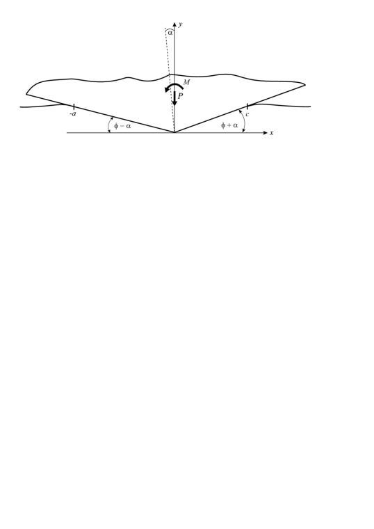
Figure 4: Tilted wedge subject to a normal load and a moment.

The contact coordinates are determined from the equilibrium equation

$$P=\int_{-a}^{c}p(x)\,\mathrm{d}x=\frac{2\phi}{A}\sqrt{ac}\;,$$ (27)

and the consistency condition (9), which here yields

$$\int_{-a}^{c}\frac{g^{\prime}(\xi)\mathrm{d}\xi}{w(\xi,a,c)}=-\pi\alpha=2\phi\,\arcsin\left(\frac{c-a}{a+c}\right)$$ (28)

[13]. These equations can be solved to give

$$a=\frac{AP}{2\phi}\sqrt{\frac{1+s}{1-s}}\;;\;\;\;c=\frac{AP}{2\phi}\sqrt{\frac{1-s}{1+s}}\rule{14.22636pt}{0.0pt}\mbox{where}\rule{14.22636pt}{0.0pt}s=\sin\left(\frac{\pi\alpha}{2\phi}\right)\;.$$ (29)

For completeness, we also give the expression for the moment $M$ which is

$$M=\int_{-a}^{c}p(x)x\,\mathrm{d}x=\frac{\phi}{A}\left(\frac{a+c}{2}\right)^{2}\left(\frac{c-a}{a+c}\sqrt{1-\left(\frac{c-a}{a+c}\right)^{2}}+\arcsin{\left(\frac{c-a}{a+c}\right)}\right)\;.$$ (30)

The coordinates $[-m,n]$ defining the permanent stick zone are then immediately determined by substituting the mapping (25) into (29), giving

$$m=\frac{A}{2\phi}\left(P_{0}-\frac{\Delta Q}{2f}\right)\sqrt{\frac{1+t}{1-t}}\;;\;\;\;n=\frac{A}{2\phi}\left(P_{0}-\frac{\Delta Q}{2f}\right)\sqrt{\frac{1-t}{1+t}}\;,$$ (31)

where

$$t=\sin\left(\frac{\pi\alpha_{0}}{2\phi}-\frac{\pi A\Delta\sigma}{16f\phi}\right)\;.$$ (32)

We can also determine the change in the corrective tractions in the permanent stick zone as

$$[q_{2}^{\ast}-q_{1}^{\ast}](x)=-\frac{4f\phi}{\pi A}\ln\left|\frac{1-\sqrt{(1-x/n)/(1+x/m)}}{1+\sqrt{(1-x/n)/(1+x/m)}}\right|\;,$$ (33)

from (26, 25).

2.5 Display of example problem results

There is a multitude of possibilities to illustrate the results of the mapping procedure. The most sensible way seems to be to present, first, different steady state solutions for a varying bulk stress, $\Delta\sigma$. Consider Figure 5 (a), note that each value of $\Delta\sigma a/\Delta Q$ represents a stand-alone steady state solution subject to a constant normal load, $P_{0}$, giving the mean contact size spanning $[-a_{0},\quad c_{0}]$ and subject to a constant shear load fluctuation, $\Delta Q$, giving the permanent stick zone spanning $[-m,\quad n]$. In this first example the wedge is indented symmetrically, i.e. $\alpha_{0}$ is kept zero and the contact extent and position are unaffected by the change in bulk stress, ($a=c=$ const.). We see that, as the change in bulk stress is increased, the permanent stick zone shifts towards the LHS contact edge. Note however, the extent of the permanent stick zone increases slightly with a bigger $\Delta\sigma$, albeit almost not visible in this example. The solution finds its limit when the boundary of the permanent stick zone and a contact edge coincide, e.g. $a=m$ or $n=c$. If the change in bulk stress is increased further from that point onwards, the contact will experience reversed slip.

Figure 5: Steady state solutions of (a) slip and stick zone extents and (b) shear tractions for different values of a change in bulk stress, $\Delta\sigma$.

In Figure 5 (b), the shear traction distribution is depicted for three particular values of $\Delta\sigma a/\Delta Q$ as the slip zones reach their maximum extent in the steady state cycle and stick is only maintained in the permanent stick zone. Note that the area underneath each shear traction distribution remains constant, i.e. $\int_{-a}^{c}q(x)\,\mathrm{d}x=$ const., and it is merely the form and slip-stick boundary that change with the steady state change in bulk stress.

We now turn to the effects of the average angles of tilt, $\alpha_{0}$. Figure 6 (a) is similar to Figure 5 (a), each value of $\alpha_{0}$ represents a stand-alone steady state solution subject to a constant normal load, $P_{0}$, giving the mean contact size spanning $[-a_{0},\quad c_{0}]$ and subject to a constant shear load fluctuation, $\Delta Q$, giving the permanent stick zone spanning $[-m,\quad n]$. Here, the fluctuation in bulk stress, $\Delta\sigma$, is kept zero as the intention is to demonstrate the effects of tilt exclusively.

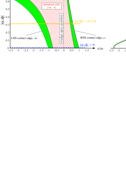
Figure 6: Steady state solutions of (a) slip and stick zone extents and (b) shear tractions for different values of a change in average angle of tilt, $\alpha_{0}$.

From Figure 6 (a) it is apparent that the normal load solution dictates the qualitative behaviour of the tangential solution. Increasing the average angle of tilt influences not only the extent and position of the contact, but also the extent and position of the permanent stick zone within the contact. In Figure 6 (b), the shear traction distribution is depicted for three particular values of $\alpha_{0}/\phi$ as the slip zones reach their maximum extent in the steady state cycle and stick is only maintained in the permanent stick zone. Note that, as in Figure 5 (b), the area underneath each shear traction distribution remains constant, i.e. $\int_{-a}^{c}q(x)\,\mathrm{d}x=$ const., and it is merely the extent, form, and slip-stick boundary that change with the average angle of tilt in the steady state.

In summary, the two above figures reflect the solution behaviour indicated by equations (31) and (32). We note that it is the mean normal load, $P_{0}$, and the average angle of tilt, $\alpha_{0}$, which affect the tangential solution, together with the tangential load inputs, $\Delta\sigma$ and $\Delta Q$.

3 Conclusions

The paper provides a comprehensive but manageable method for finding the size of the permanent stick zone for the problem of a general half plane contact subject to a constant set of loads ($P,Q,M,\sigma$) together with periodic changes in these same quantities.

The solution is appropriate when the bulk stress is never high enough to reverse the sense of slip at a contact edge, and applies in the steady state. We found that the permanent stick zone is independent of the mean loads of shear $Q_{0}$ and bulk tension $\sigma_{0}$, but rather depends on $P_{0}$, $\Delta Q$, $\Delta\sigma$, and the average angle of tilt, $\alpha_{0}$. A straightforward way of using the full solution for normal load to find the size of the permanent stick zone is developed which requires no further work or algebra to be carried out. The method is applied explicitly to the problem of a wedge as this permits all the algebraic steps needed to be displayed. Its application to the more frequent practically occurring ‘flat and rounded’ contact case is straightforward, if algebraically more taxing.

As we are interested in the maximum extent of the slip zones during the steady state, ($a_{i}-m$) and ($c_{i}-n$), we need $\Delta P$ and $\Delta M$ as additional inputs for the normal load problem in order to obtain the contact coordinates at load points 1 and 2, $[-a_{i},\quad c_{i}]$, for $i=1,2$. However, these additional inputs and outputs are not required for carrying out the mapping procedure and finding the permanent stick zone.

References

- [1] H. Andresen, D. Hills, J. Barber, J. Vázquez, Frictional half-plane contact problems subject to alternating normal and shear loads and tension in the steady state, Int. Jnl. Solids Struct. (in press, DOI: j.ijsolstr.2019.03.025) (2019).
- [2] H. Hertz, über die berührung fester elastischer körper, Journal für die reine und angewandte Mathematik 92 (1881) 156–171 (1881).
- [3] C. Cattaneo, Sul contato di due corpo elastici, Atti Accad. Naz. Lincei, Cl. Sci. Fis., Mat. Nat., Rend. 27 (1938) 342–348, 434–436, 474–478 (1938).
- [4] R. Mindlin, Compliance of elastic bodies in contact, AASME Trans. Jnl. Appl. Mech. 16 (1949) 259–268 (1949).
- [5] R. Mindlin, W. Mason, T. Osmer, H. Dereiewicz, Effect of an oscillating tangential force on the contact surfaces of elastic spheres, Proc. First Nat. Congress of Applied Mechanics (1951) 203–208 (1951).
- [6] R. Mindlin, H. Dereiewicz, Elastic spheres in contact under varying oblique forces, J. of Applied Mechanics 20 (1953) 327–344 (1953).
- [7] D. Hills, D. Nowell, Mechanics of fretting fatigue tests, Int. Jnl. Mech. Sci. 29 (1987) 355–365 (1987).
- [8] J. Jäger, A new principle in contact mechanics, Jnl. Tribology 120 (1998) 677–684 (1998).
- [9] M. Ciavarella, The generalised cattaneo partial slip plane contact problem, part i theory, part ii examples, Int. Jnl. Solids Struct. 35 (1998) 2349–2378 (1998).
- [10] J. Barber, M. Davies, D. Hills, Frictional elastic contact with periodic loading, Int. Jnl. Solids Struct. 48 (2011) 2041–2047 (2011).
- [11] D. Hills, D. Nowell, A. Sackfield, Mechanics of Elastic Contacts, Butterworth-Heinemann, 1993 (1993).
- [12] A. Sackfield, C. Truman, D. Hills, The tilted punch under normal and shear load (with application to fretting tests), Int. Jnl. Mech. Sci. 43 (2001) 1881–1892 (2001).
- [13] A. Sackfield, D. Dini, D. Hills, The tilted shallow wedge problem, European Journal of Mechanics A/Solids 24 (2005) 919–928 (2005).