A Full Quantum Eigensolver for Quantum Chemistry Simulations

Quantum simulation of quantum chemistry is one of the most compelling applications of quantum computing. It is of particular importance in areas ranging from materials science, biochemistry and condensed matter physics. Here, we propose a full quantum eigensolver (FQE) algorithm to calculate the molecular ground energies and electronic structures using quantum gradient descent. Compared to existing classical-quantum hybrid methods such as variational quantum eigensolver (VQE), our method removes the classical optimizer and performs all the calculations on a quantum computer with faster convergence. The gradient descent iteration depth has a favorable complexity that is logarithmically dependent on the system size and inverse of the precision. Moreover, the FQE can be further simplified by exploiting perturbation theory for the calculations of intermediate matrix elements, and obtain results with a precision that satisfies the requirement of chemistry application. The full quantum eigensolver can be implemented on a near-term quantum computer. With the rapid development of quantum computing hardware, FQE provides an efficient and powerful tool to solve quantum chemistry problems.

I introduction

Quantum chemistry studies chemical systems using quantum mechanics. One primary focus of quantum chemistry is the calculation of molecular energies and electronic structures of a chemical system which determine its chemical properties. Molecular energies and electronic structures are calculated by solving the Schrödinger equation within chemical precision. However, the computational resources needed scale exponentially with the system size on a classical computer, making the calculations in quantum chemistry intractable in high-dimension.

Quantum computers, originally envisioned by Benioff, Manin and Feynman benioff1980computer ; manin1980vychislimoe ; feynman1982simulating , have emerged as promising tools for tackling this challenge with polynomial overhead of computational resources. Efficient quantum simulations of chemistry systems promise breakthroughs in our knowledge for basic chemistry and revolutionize research in new materials, pharmaceuticals, and industrial catalysts.

The universal quantum simulation method lloyd1996universal and the first quantum algorithm for simulating fermions abrams1997simulation have laid down the fundamental block of quantum chemistry simulation. Based on these techniques and quantum phase estimation algorithm kitaev1995quantum , Aspuru-Guzik et al presented a quantum algorithm for preparing ground states undergoing an adiabatic evolution aspuru2005simulated , and many theoretical and experimental works babbush2014adiabatic ; feng2013experimental ; lu2015experimental ; babbush2015chemical ; wei2016dualityopen ; babbush2016exponentially ; babbush2017exponentially ; kassal2008polynomial ; kivlichan2017bounding ; toloui2013quantum ; peruzzo2014variational ; mcclean2016theory ; mcclean2014exploiting ; whitfield2011simulation ; wecker2015progress ; hastings2014improving ; kyriienko2019quantum have been developed since then. In 2002, Somma et al. proposed a scalable quantum algorithm for the simulation of molecular electron dynamics via Jordan-Wigner transformation jordan1928pauli . The Jordan-Wigner transformation directly maps the fermionic occupation state of a particular atomic orbital to a state of qubits, which enables the quantum simulation of chemical systems on a quantum computer. Then, the Bravyi-Kitaev transformation bravyi2002fermionic ; seeley2012bravyi ; tranter2015b ; bravyi2017tapering ; babbush2018low encodes both locality of occupation and parity information onto the qubits, which is more efficient in operation complexity. In 2014, Peruzzo et al developed the variational quantum eigensolver (VQE) peruzzo2014variational ; yung2014transistor , which finds a good variational approximation to the ground state of a given Hamiltonian for a particular choice of ansatz. Compared to quantum phase estimation and trotterization of the molecular Hamiltonian, VQE requires a lower number of controlled operations and shorter coherence time. However, VQE is a classical and quantum hybrid algorithm, the optimizer is performed on a classical machine.

Meanwhile, implementations of quantum chemistry simulation have been developing steadily. Studies in present-day quantum computing hardware have been carried out, such as nuclear magnetic resonance system du2010nmr ; li2019quantum , photonic system roushan2017chiral ; lanyon2010towards ; paesani2017experimental , nitrogen-vacancy center system wang2015quantum , trapped ion shen2017quantum ; hempel2018quantum and superconducting system o2016scalable ; kandala2017hardware ; ganzhorn2019gate . Rapid development in quantum computer hardware with even the claims of quantum supremacy, greatly stimulates the expectation of its real applications. Quantum chemistry simualtion is considered as a real application in Noisy Intermediate-Scale Quantum (NISQ) computers mohseni2017commercialize ; wecker2015progress ; mueck2015quantum . The FQE is an effort on this background. In FQE, not only calculation of Hamiltonian matrix part is done on quantum computer, but also the optimization by gradient descent is performed on quantum computer. FQE can be used in near-term NISQ computers, and in future fault-tolerant large quantum computers.

II method

II.1 Preparing the Hamiltonian for Quantum Chemistry Simulation

A molecular system, contains a collection of nuclear charges $Z_{i}$ and electrons. The fundamental task of quantum chemistry is to solve the eigenvalue problem of the molecular Hamiltonian. The eigenstates of the many-body Hamiltonian determine the dynamics of the electrons as well as the properties of the molecule. The corresponding Hamiltonian of the system includes kinetic energies of nuclei and electrons, the Coulomb potentials of nuclei-electron, nuclei-nuclei, electron-electron and it can be expressed in first quantization as

$$H_{o} =-\sum_{i}\frac{\nabla_{R_{i}}^{2}}{2M_{i}}-\sum_{i}\frac{\nabla_{r_{i}}^{2}}{2}-\sum_{i,j}\frac{Z_{i}}{|R_{i}-r_{j}|}$$ (1)

$$+\sum_{i,j>i}\frac{Z_{i}Z_{j}}{|R_{i}-R_{j}|}+\sum_{i,j>i}\frac{1}{|r_{i}-r_{j}|},$$

in atomic units $(\hbar=1)$, where $R_{i},Z_{i},M_{i}$ and $r_{i}$ are the positions, charges, masses of the nuclei and the positions of the electrons respectively. Under the Born-Oppenheimer approximation which assumes the nuclei as a fixed classical point, this Hamiltonian is usually rewritten in the particle number representation in a chosen basis

$$H=\sum_{ij}h_{ij}a^{\dagger}_{i}a_{j}+\frac{1}{2}\sum_{ijkl}h_{ijkl}a^{\dagger}_{i}a^{\dagger}_{j}a_{k}a_{l}+\dots,$$ (2)

where $\cdots$ denotes higher order interactions and $a_{i}^{\dagger}$ and $a_{j}$ are the creation and annihilation operator of particle in orbital $i$ and $j$ respectively. The parameters $h_{ij}$ and $h_{ijkl}$ are the one-body and two-body integrations in the chosen basis functions $\{\psi_{i}\}$. In Galerkin formulation, the scalar coefficients in Eq. (2) can be calculated by

$$h_{ij} =\langle\psi_{i}|\left(-\frac{\nabla_{i}^{2}}{2}-\sum_{A}\frac{Z_{A}}{\left|r_{i}-R_{A}\right|}\right)|\psi_{j}\rangle$$ (3)

$$h_{ijkl} =\langle\psi_{i}\psi_{j}|\frac{1}{\left|r_{i}-r_{j}\right|}|\psi_{k}\psi_{l}\rangle$$

In order to perform calculations on a quantum computer, we need to map fermionic operators to qubit operators. We choose Jordan-Wigner transformation to achieve this task due to its straightforward expression.

The Jordan-Wigner transformation maps Eq. (2) into a qubit Hamiltonian form

$$H= \sum_{i,\alpha}h_{\alpha}^{i}\sigma_{\alpha}^{i}+\sum_{i,j,\alpha,\beta}h_{\alpha\beta}^{ij}\sigma_{\alpha}^{i}\sigma_{\beta}^{j}+\dots,$$ (4)

where Roman indices $i,j$ denote the qubit on which the operator acts, and Greek indices $\alpha,\beta$ refer to the type of Pauli operators, i.e., $\sigma^{i}_{x}$ means Pauli matrix $\sigma_{x}$ acting on a qubit at site $i$. Apparently, $H$ in Eq. (2) is a linear combination of unitary Pauli matrices. The methods used in this paper finding the molecular ground-state and its energy are all based on it.

In this work, we present the FQE to find the molecular ground-state energy by gradient descent iterations. Gradient descent is one of the most fundamental ways for optimization, that looks for the target energy value along the direction of the steepest descent. Here it is performed in a quantum computer with the help of linear combination of unitary operators. We analyse the relationships between the gradient descent iteration depth and the precision of the ground-state energy. The explicit quantum circuit to implement the algorithm is constructed. As illustrative examples, the ground-state energies and electronic structures of four molecules, H₂, LiH, H₂O and NH₃ are presented. Taking H₂O and NH₃ as examples, a comparison between the FQE and VQE, a representative hybrid method, is given. FQE can be accelerated further by harnessing perturbation theory in chemical precision. Finally, we analyse the computation complexity of FQE and summarize the results.

II.2 Quantum Gradient Descent Iteration

The classical gradient descent algorithm is usually employed to obtain the minimum of an target function $f(\mathbf{X})$. One starts from an initial point $\mathbf{X}^{(0)}={x_{1}^{0},x_{2}^{0},\dots,x_{N}^{0}}\in\mathbb{R}^{N}$, then moves to the next point along the direction of the gradient of the target function, namely

$$\mathbf{X}^{(t+1)}=\mathbf{X}^{(t)}-\gamma_{0}\nabla f(\mathbf{X}^{(t)}),$$ (5)

where $\gamma_{0}$ is a positive learning rate that determines the step size of the iteration. In searching the minimum energy of a Hamiltonian, the target function can be expressed as a quadratic optimization problem in the form, $f(\mathbf{X})=\mathbf{X}^{T}\mathbf{H}\mathbf{X}$. At point $\mathbf{X}$, the gradient operator of the objective function can be expressed as

$$\nabla f(\mathbf{X})=2\mathbf{H}\mathbf{X}.$$ (6)

Then, the gradient descent iteration can be regarded as an evolution of $\mathbf{X}$ under operator $\mathbf{H}$,

$$|\mathbf{X}^{(t+1)}\rangle=\left(|\mathbf{X}^{(t)}\rangle-\gamma\mathbf{H}|\mathbf{X}^{(t)}\rangle\right),$$ (7)

where $\gamma_{0}$ is redefined as $\gamma=2\gamma_{0}$. In quantum gradient descent, vector $\mathbf{X}$ is replaced by quantum state $|\mathbf{X}\rangle=\sum_{j}x_{j}|j\rangle/\|\mathbf{X}\|$, where $x_{j}$ is the $j$-th elements of the vector, $|j\rangle$ is the $N$-dimensional computational basis, and $\|\mathbf{X}\|$ is the modulus of vector $\mathbf{X}$. Denoting $\mathbf{H}^{g}=\mathbf{I}-\gamma\mathbf{H}$ and it can be expressed as

$$\mathbf{H}^{g}=\sum_{i=1}^{M}\beta_{i}\mathbf{H}^{g}_{i},$$ (8)

where $M$ is the number of Pauli product terms in $\mathbf{H}^{g}$. Then the gradient descent process can be rewritten as

$$|\mathbf{X}^{(t+1)}\rangle=\mathbf{H}^{g}|\mathbf{X}^{(t)}\rangle=\sum_{i=1}^{M}\beta_{i}\mathbf{H}^{g}_{i}|\mathbf{X}^{(t)}\rangle,$$ (9)

where $\mathbf{H}^{g}$ is a linear combination of unitary operators(LCU) which was proposed in gui2006general in designing quantum algorithms and studied extensively gudder2007mathematical ; gui2008duality ; gui2009allowable ; long2011duality ; childs2012hamiltonian ; berry2015simulating ; wei2016duality . This non-unitary evolution can be implemented in a unitary quantum circuit by adding ancillary qubits that transform it into unitary evolution in a larger space cao2010restricted . The realization of LCU can be viewed as a quantum computer wavefunction passing through M-slits, and operated by a unitary operation in each slit, and then the wavefunctions are combined and the result of the calculation is readout by a measurement long2011duality . We perform the evolution described by Eq. (9) with the following four steps.

Wave division: The register is a composite system which contains a work system and an ancillary register. Firstly, the initial point $\mathbf{X}=(x_{1},\dots,x_{N})^{T}$ is efficiently mapped as an initial state $|\mathbf{x}^{(t)}\rangle$ of the work system. In quantum chemistry, Hartree-Fock (HF) product state is usually used as an initial state. And the ancillary register is initialized from $|0\rangle^{m}$, where $m=\text{log}_{2}M$, to a specific superposition state $|\psi_{s}\rangle$,

$$|\psi_{s}\rangle=\frac{1}{\mathbb{C}}\sum_{i=0}^{M-1}\beta_{i}|i\rangle$$ (10)

where $\mathbb{C}=\sqrt{\sum_{i=0}^{M-1}\beta_{i}^{2}}$ is a normalization constant and $|i\rangle$ is the computational basis. This is equivalent to let the state $|\mathbf{x}^{(t)}\rangle$ pass through M-slits. $\beta_{i}$ is a factor describing the properties of the slit, which is determined by the forms of the Hamiltonian in Eq. (8). This can be done by the initialization algorithm in long2001efficient . Moreover, the quantum random access memory (qRAM) approach can be used to prepare $|\mathbf{x}^{(t)}\rangle$ and $|\psi_{s}\rangle$, which consume $O(\log N)$ and $O(\log M)$ basic steps or gates respectively after qRAM cell is established. We denote the whole state of the composite system as $|\Phi\rangle=|\psi_{s}\rangle|\mathbf{x}^{(t)}\rangle$.

Entanglement: Then, a series of ancillary system controlled operations $\sum_{i=0}^{M-1}|i\rangle\langle i|\otimes H^{g}_{i}$ are implemented on the work qubits. The work qubits and the ancilla register are now entangled , and the state is transformed into

$$|\Phi\rangle\rightarrow\frac{1}{\mathbb{C}}\big{(}\sum_{i=0}^{M-1}\beta_{i}|i\rangle H^{g}_{i}|\mathbf{x}^{(t)}\rangle\big{)}.$$ (11)

The corresponding physical picture is that different unitary operations are implemented simultaneously in different subspaces, corresponding to different slits.

Wave combination : We perform $m$ Hadamad gates on ancillary register to combine all the wavefunctions from the $M$ different subspaces. We merely focus on the component in a subspace where the ancillary system is in state $|0\rangle$. The state of the whole system in this subspace is

$$|\Phi_{0}\rangle=\frac{1}{\mathbb{C}\sqrt{2^{m}}}\big{(}|0\rangle\sum_{i=0}^{M-1}\beta_{i}H^{g}_{i}|\mathbf{x}^{(t)}\rangle\big{)}.$$ (12)

Measurement: Then, we measure the ancillary register. If we obtain $|0\rangle$, our algorithm succeeds and we obtain the state $\frac{1}{\mathbb{C}\sqrt{2^{m}}}\big{(}|0\rangle\sum_{i=0}^{M-1}\beta_{i}H^{g}_{i}|\mathbf{x}^{(t)}\rangle\big{)}$, where the work system is in $|\mathbf{x}^{(t+1)}\rangle=\mathbf{H}^{g}|\mathbf{x}^{(t)}\rangle$. And then this will be used as input for the next iteration in the quantum gradient descent process. The probability of obtaining $|0\rangle$ for the state is

$$P_{s}=\parallel\mathbf{H}^{g}|\mathbf{x}^{(t)}\rangle\parallel^{2}/{\mathbb{C}^{2}M}.$$

The successful probability after $n$ measurements is $1-(1-\frac{\parallel\mathbf{H}^{g}|\mathbf{x}^{(t)}\rangle\parallel^{2}}{\mathbb{C}^{2}M})^{n}$, which is an exponential function of $n$. The number of measurements is ${\mathbb{C}^{2}M}/\parallel\mathbf{H}^{g}|\mathbf{x}^{(t)}\rangle\parallel^{2}$. The measurement complexity will grow exponentially with respect to the number of iteration steps rebentrost2019quantum . Alternatively, one can use the oblivious amplitude amplification berry2015simulating to amplify the amplitude of the desired term (ancillary qubits in state $|0\rangle$) up to a deterministic order with $O(\sqrt{M})$ repetitions before the measurement. Then, the measurement complexity will be the product of iteration depth $k$ and $O(\sqrt{M})$, linearly dependent on the number of iteration steps. After obtaining $|0\rangle$, we can continue the gradient descent process by repeating the above four steps, with $|\mathbf{x}^{(t)}\rangle$ repalced by $|\mathbf{x}^{(t+1)}\rangle$ in Wave-division step. We can pre-set a threshold defined as $\varepsilon=|\langle\mathbf{x}_{t}|H|\mathbf{x}_{t}\rangle-\langle\mathbf{x}_{t+1}|H|\mathbf{x}_{t+1}\rangle|/\langle\mathbf{x}_{t}|H|\mathbf{x}_{t}\rangle$ as criterion for stopping the iteration. Thus, we judge if the iterated state satisfies criterion by measuring the expectation value of Hamiltonian around the expected number of iteration, which is easier than constructing the tomography. If the next iterative state $|\mathbf{x}^{(t+1)}\rangle$ does not hit our pre-set threshold, this output $|\mathbf{x}^{(t+1)}\rangle$ will be regarded as the new input state $|\mathbf{x}^{(t)}\rangle$ and run the next iteration. Otherwise, the iteration can be terminated and the state $|\mathbf{x}^{(t+1)}\rangle$ is the final result $|\mathbf{x}_{f}\rangle$, as one good approximation of the ground state. The ground state energy can be calculated by $\langle\mathbf{x}_{f}|H|\mathbf{x}_{f}\rangle$.

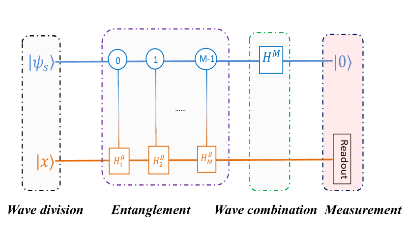
Figure 1: Quantum circuit for gradient descent. $|\mathbf{x}\rangle$ and $|\psi_{s}\rangle$ denote the initial state of the work system and ancilla syetem respectively. The controlled operations acted on work system are $\sum_{i=0}^{M-1}|i\rangle\langle i|\otimes H^{g}_{i}$. $H^{M}$ denotes $m=\text{log}_{2}M$ number Hadamard gates.At the end of the circuit, we measure the final state of the ancilla registers. If all ancilla qubits are $|0\rangle$, the work systerm collapses into state $|\mathbf{x}^{(t+1)}\rangle$.

Measuring the expectation values during the iteration procedure will destroy the state of the work system, stopping the quantum gradient descent process. So, determing the iteration depth $k$ in advance is essential. After $k$ times iterations, the approximation error is limited to (ignoring constants)

$$\epsilon\leq O\left((\frac{1-\gamma\lambda_{2}}{1-\gamma\lambda_{1}})^{k}N\right),$$

where $\lambda_{1}$ and $\lambda_{2}$ are the two largest absolute values of the eigenvalues of Hamiltonian $\mathbf{H}$ (see Supplemental Material for proof). The iteration depth

$$k=O(\log\frac{N}{\epsilon})$$ (13)

is logarithmically dependent on the system size and the inverse of precision. The algorithm may be terminated at a point with a pre-set precision $\epsilon$. It can be seen that the choise of $\gamma$ has little impact on converge rate when $\gamma$ is large. This makes this algorithm very robust to this parameter. The rate of convergence primarily depends upon the ratio of $\lambda_{1}$ and $\lambda_{2}$. The gap between the iterative result and the ground state depends on the choice of initial point. If we choose an ansatz state with a large overlap with the exact ground state, the iterative process will converge to the the ground state in fewer iterations. Usually, the mean-field state which represents a good classical approximation to the ground state of Hamiltonian H, such as a Hartree-Fock (HF) product state, is chosen as an initial state. Compared to VQE, FQE does not need to make measurements of the expectation values of Hamiltonian during each iteration procedure and this substantially reduces the computation resources.

II.3 Perturbation Theory

The FQE involves multi-time iterations to obtain an accurate result, which is difficult to implement in the present-day quantum computer hardware. Here, we present an approximate method to find the ground state and its energy by using the gradient descent algorithm and perturbation theory. Perturbation theory is widely used and plays an important role in describing real quantum systems, because it is impossible to find exact solutions to the Schrödinger equation for Hamiltonians even with moderate complexity. The Hamiltonian described by Eq. (4) can be divided into two classes, $\mathbf{H}_{0}$ and $\mathbf{H}^{\prime}$. $\mathbf{H}_{0}$ consists of a set of Pauli terms containing only $\sigma^{i}_{\alpha=z}$ and the identity matrices, and Pauli terms $\sigma^{i}_{\alpha=x,y}$ belong to $\mathbf{H}^{\prime}$. $\mathbf{H}_{0}$ is a diagonal matrix with exact solutions, that can be regarded as a simple system. $\mathbf{H}^{\prime}$ usually is smaller compared to $\mathbf{H}_{0}$, and is treated as a “perturbing” Hamiltonian. The energy levels and eigenstates associated with the perturbed system can be expressed as “corrections” to those of the unperturbed system. We begin with the time-independent Schrödinger equation:

$$\mathbf{H}|\psi_{n}\rangle=(\mathbf{H}_{0}+\mathbf{H}^{\prime})|{\psi}_{n}\rangle=E_{n}|{\psi}_{n}\rangle,$$ (14)

where $E_{n}$ and $|\psi_{n}\rangle$ are the n-th energy and eigenstate respectively. Unperturbed Hamiltonian $\mathbf{H}_{0}$, satisfies the time-independent Schrödinger equation: $\mathbf{H}_{0}|n\rangle=E_{n}^{(0)}|n\rangle$. Our goal is to express $E_{n}$ and $|\psi_{n}\rangle$ in terms of $E_{n}^{0}$ and $|n\rangle$. Denote the expectation value of $\mathbf{H}^{\prime}$ as $\mathbf{H}^{\prime}_{nn}=\langle{n}|\mathbf{H}^{\prime}|{n}\rangle$, and it is easily to see that $\langle{n}|\mathbf{H}^{\prime}|{n}\rangle$ is zero because $\mathbf{H}^{\prime}$ only contains Pauli terms $\sigma^{i}_{\alpha=x,y}$. In the first order approximation, the energies and eigenstates are expressed as

$$E_{n} =E_{n}^{(0)},$$ (15)

$$|\psi_{n}\rangle =|{n}\rangle-\sum_{m\neq n}\frac{\mathbf{H}^{\prime}_{mn}}{E_{m}^{(0)}-E_{n}^{(0)}}|m\rangle.$$ (16)

To second-order approximation, they are

$$E_{n} =E_{n}^{(0)}+\sum_{m\neq n}\frac{|\mathbf{H}^{\prime}_{mn}|^{2}}{E_{m}^{(0)}-E_{n}^{(0)}},$$ (17)

$$|\psi_{n}\rangle =|{n}\rangle-\sum_{m\neq n}\frac{\mathbf{H}^{\prime}_{mn}}{E_{m}^{(0)}-E_{n}^{(0)}}|m\rangle-\frac{1}{2}\sum_{m\neq n}\frac{|\mathbf{H}^{\prime}_{mn}|^{2}}{(E_{m}^{(0)}-E_{n}^{(0)})^{2}}|n\rangle,$$ (18)

$$+\sum_{m\neq n}\left[\sum_{k\neq n}\frac{\mathbf{H}^{\prime}_{mn}\mathbf{H}^{\prime}_{kn}}{(E_{m}^{(0)}-E_{n}^{(0)})(E_{k}^{(0)}-E_{n}^{(0)})}\right]|m\rangle.$$

The matrix elements in the first and second-order approximations can be obtained by one iteration of the quantum circuit in Fig.1. Here, we let $\mathbf{H}^{\prime}$ be equal to $\mathbf{H}^{g}$. Explicitly, the first order approximation only involves $\mathbf{H}^{\prime}_{mn}$, a series of transition probabilities of the state after $\mathbf{H}^{\prime}$ implemented on state $|{n}\rangle$, and they can be obtained by performing the quantum circuit of Fig.1 directly. For the second order approximation, matrix elements such as value $|\mathbf{H}^{\prime}_{mn}|^{2}$ and $\mathbf{H}^{\prime}_{mn}\mathbf{H}^{\prime}_{kn}$, can be calculated by $\mathbf{H}^{\prime}_{mn}$. Then, the approximate ground energy and ground state up to second-order are obtained. We will show the performance of FQE and perturbation theory in next section.

III results

III.1 Calculations of Four Molecules

To demonstrate the feasibility of this FQE with gradient descent iteration, we carried out calculations on the ground state energy of H₂, LiH diatomic molecules, and two relatively complex molecules H₂O and NH₃. We used a common molecular basis set, the minimal STO-3G basis. Via Jordan-Wigner transformation, the qubit-Hamiltonians of these molecules are obtained. The Hamiltonians of H₂, LiH, H₂O and NH₃ contain 15 , 118, 252, and 3382 Pauli matrix product terms respectively. The dimensions of the Hamiltonians of H₂, LiH, H₂O and NH₃ are 16 , 64, 4096, and 16384 respectively, which corresponds 4, 6, 12, 14 number of qubits respectively. In all four simulations, the work system was initialized to the HF state $|\mathbf{x}_{h}\rangle$ and the learning rate is chosen as $\gamma=1$. As shown in Fig.2, after about 120 iterations, the molecular energy of H₂O converges to -74.94 a.u, only $0.0013346\%$ discrepancy with respect to the exact value of -74.93 a.u. obtained via Hamiltonian diagonalization. The NH₃ calculation yields (-55.525 a.u.) after 80 iterations, matched very well with the diagonalization (-55.526 a.u.). For the study of atomic molecular structures and chemical reactions, these results are sufficiently accurate. For more complex basis set STO-6G, the results are about the same, and the details are given in Supplemental Material. The converge rates of the four molecules depend on the system size and the ratio of the two largest absolute eigenvalues of the Hamiltonian $\mathbf{H}$, which are consistent with the theoretical analysis above.

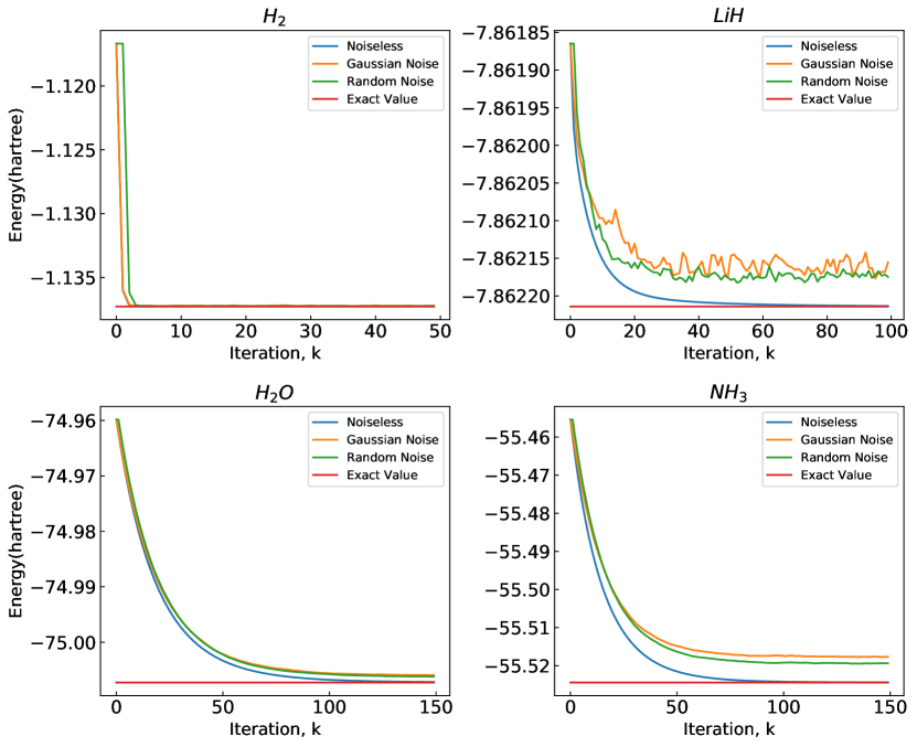
Figure 2: (a), (b), (c) and (d) show the convergence to ground state energies by FQE for H₂, LiH, H₂O and NH₃ molecules respectively. The numerical simulations are carried out with fixed interatomic distance. The exact value corresponding to Hamiltonian diagonalization energy (red line). The initial state is chosen as Hartree-Fock product state in all four cases. The final values of the lines for exact ground state energy (red line) and for the three iteration results, noiseless case (blue line), random noisy case (green line) and Gaussian noisy case (orange line).

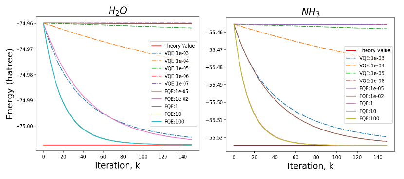
Figure 3: The exact comparison of FQE and VQE for searching ground state energy of H₂O and NH₃ molecules respectively. The red color lines labled as ’Theory Value’ are the exact values of ground state energy. The labels of the right symbols denote different learning rates.

We also studied the infulence of noises which is also shown in the Fig.2. The noise term is chosen the form of $\sum_{i=1}^{N}\delta\alpha_{i}\sigma_{z}$ , added to the Hamiltonian to simulate decoherence. Then we add a term $|\delta\vec{x}\rangle$ on the iterative state $|\mathbf{x}^{k}\rangle$ to simulate measurement error and renormalize the iterative state as $|\mathbf{x}^{(k)}\rangle\rightarrow(|\mathbf{x}^{(k)}\rangle+|\delta\vec{x}\rangle)/\parallel|\mathbf{x}^{(k)}\rangle+|\delta\vec{x}\rangle\parallel$. We set a random noise ( amplitude $0.01$) and a Gaussian noise ($\mu=0,\sigma=0.01/3$) for H₂ and LiH. For H₂O and NH₃, we choose a random noise (amplitude $0.02$) and a Gaussian noise ($\mu=0,\sigma=0.02/3$). The results still converge to the exact values in chemical precision ($1.6\times 10^{-3}$ a.u). This indicates that our method is robust to certain type of noise, which is important in the implementation of quantum simulation on near term quantum devices. For more noisy situations, see Supplemental Material for details, where the parameters of noise are 10 times of the above values. The convergence deteriorates and some oscillations accur as the number of iterations increases.

In Fig.3, a comparison with VQE is shown for H₂O and NH₃. In VQE calculation, the initial state $|\mathbf{x}_{0}\rangle$ is mapped to an ansatz state by a parameterized unitary operation $|\mathbf{x}({\vec{\theta}})\rangle=U(\vec{\theta})|\mathbf{x}_{0}\rangle$. VQE solves for the parameter vector $\vec{\theta}$ with a classical optimization routine. Here we adopt the standard gradient descent method as the classical optimizer in VQE. The parameter is updated by $\vec{\theta}\rightarrow\vec{\theta}-\gamma\frac{f(\vec{\theta}+\Delta\vec{\theta})-f(\vec{\theta})}{\Delta\vec{\theta}}$. We performed numerical simulations of VQE for the two molecules. When the learning rate $\gamma\geq 10^{-3}$, VQE does not converge to the ground state. So, in order to compare with each other, we choose the proper learning rates in two methods seperately. In both cases, the initial ansatz state is prepared as the HF product state. In H₂O and NH₃, VQE converges most fast with the learning rate $\gamma=10^{-3}$. FQE converges more and more fast with larger and larger learning rate until a fixed speed is reached . As shown in Fig.3, FQE generally converges faster than VQE and the advantage will be more obvious in complex molecules.

The above examples are calculated in fixed interatomic distance of the molecules. If we want to calculate the interatomic distance corresponding to the most stable structure, the variation of interatomic distances is necessary. In Fig.4, four examples are given to illustrate the performance of perturbation theory. To obtain the potential-energy surfaces for H₂, LiH, H₂O and NH₃ molecules, we studied the dependence of ground-state energy of their molecules on the variating interatomic distances, between the two atoms in H₂, LiH, and the distance between the oxygen atom and one hydrogen atom (the two hydrogen atoms are symmetric with respect to the oxygen atom) in H₂O, and the distance between the nitrogen atom and the plane formed by the three hydrogen atoms in NH₃. The lowest energy in potential-energy surfaces corresponds to the most stable structure of the molecules. As shown in the picture, the ground-state energy of each molecule calculated under the second order approximation are already quite close to their exact values, which is obtained from Hamiltonian diagonalizations. The energy values up to second-order correction are compared with their exact values at the most stable interatomic distance corresponding to the lowest energy in Table.1. It can be seen that the second order approximation has already given results in chemical precision.

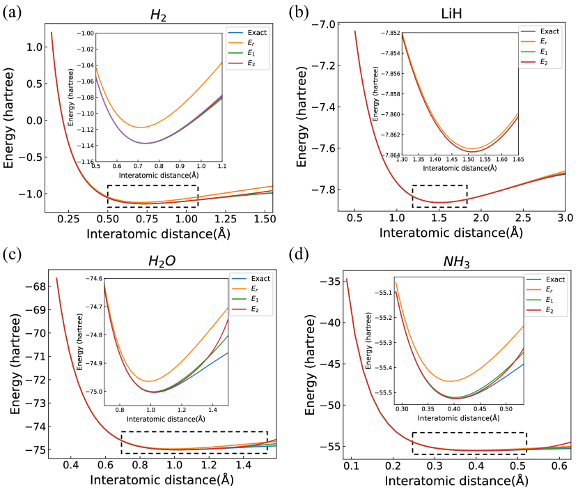
Figure 4: Theory results (blue lines), zero-order (orange lines), first-order (green lines) and second-order (red lines) energy plots of outcomes from numerical simulations, for several interatomic distances for H₂, LiH, H₂O (between the oxygen atom and one hydrogen atom) and NH₃ (between the nitrogen atom and the plane formed by the three hydrogen atoms).

	exact value	zero-order value	first-order value	second-order value
H2(0.7314)	-1.1373	-1.1171	-1.1372	-1.1372
LiH(1.5065)	-7.8637	-7.8634	-7.8637	-7.8637
H2O(1.0812)	-75.0038	-74.9622	75.0013	75.0032
NH3(0.4033)	-55.5247	-55.4530	-55.5193	-55.5237

Table 1: Energy values calculated by perturbation method and the exact values in the most stable distance corresponding to the lowest ground energy.

III.2 Analysis of Computational Complexity

Here we analyze the complexity of our algorithm. Usually, a quantum algorithm complexity involves two aspects: qubit resources and gate complexity. For qubit resources, the number of ancilla qubits is $\text{log}M$, where $M$ is the number of Pauli terms in qubit form Hamiltonian. For gate complexity, the “Wave division” part needs $\mathcal{O}(\text{log}N+\text{log}M)$ basic steps for state preparation. The dominate factor is the number of controlled operations in “Entanglement” part in Fig. 1. Controlled $\mathbf{H}^{g}_{i}$ can be decomposed into $\mathcal{O}(M\text{log}M\text{log}N)$ basic gates xin2017quantum ; wei2018efficient . The “Wave combination ” part just comprises $\text{log}M$ Hadamard gates. Totally, FQE requires in each iteration about $\mathcal{O}(M\text{log}M\text{log}N)$ basic gates for implementation. If the wavefunction is expressed by $O(N)$ Gaussian orbitals, fermion Hamiltonians contain $O(N^{4})$ second-quantized terms, consequently the qubit Hamiltonians have $M=O(N^{4})$ Pauli terms. The qubit resource and gate complexity can be reduced to $O(N)$ and $O(N^{4})$ respectively. In some applications, the perturbation theory only requires one iteration, and an approximate result in chemical precision can be obtained.

IV Summary

An efficient quantum algorithm, Full Quantum Eigensolver (FQE), for calculating the ground state wavefunction and the ground energy using gradient descent (FQE) was proposed, and numerical simulations are performed for four molecules. In FQE, the complexity of basic gates operations is polylogarithmical to the number of single-electron atomic orbitals. It achieves an exponential speedup compared with its classical counterparts. It has been shown that FQE is robust against noises of reasonable strengths. For very noisy situations that do not allow many iterations, FQE can be combined with perturbation theory that give the ground state and its energy in chemical precision with one time iteration. FQE is exceptionally useful in quantum chemistry simulation, especially for the near-term NISQ applications. FQE is a full quantum algorithm, not only applicable for NISQ computers, but directly applicable for future large-scale fault-tolerant quantum computers.

Acknowledgements
This research was supported by National Basic Research Program of China. We gratefully acknowledges support from the National Natural Science Foundation of China under Grants No. 11974205, and No. 11774197. The National Key Research and Development Program of China (2017YFA0303700); The Key Research and Development Program of Guangdong province (2018B030325002); Beijing Advanced Innovation Center for Future Chip (ICFC).
Author contributions
S.J.W conceived the algorithm. H.L performed classical simulations. G.L.L initialized LCU scheme. All authors contributed to the discussion of results and writing of the manuscript.
Competing interests
The authors declare no competing interests.
Data availability
The data that support the findings of this study are available from the corresponding authors on reasonable request.

V Supplemental Material

V.1 Error estimation and iteration complexity

We analyse FQE’s convergence and estimate the approximation error and iteration complexity panju2011iterative . Define $|\psi_{i}\rangle$ as an normalized eigenvector for $\mathbf{H}\in\mathbb{R}^{n\times n}$ with eigenvalue $\lambda_{i}$, $\mathbf{H}|\psi_{i}\rangle=\lambda_{i}|\psi_{i}\rangle$. Suppose that $\mathbf{H}$ has real and distinct eigenvalues set $\{\lambda_{i}\}$ such that $\left|\lambda_{1}\right|>\left|\lambda_{2}\right|>\ldots>\left|\lambda_{n}\right|$. We can express an arbitrary state $|\psi\rangle$ as a linear combination of the eigenvectors of $H$:

$$|\psi\rangle=a_{1}|\psi_{1}\rangle+\ldots+a_{n}|\psi_{n}\rangle.$$

Define matrix $\mathbf{H}^{g}=\mathbf{I}-\gamma\mathbf{H}$ and perform it on $|\psi\rangle$, we have

$$\mathbf{H}^{g}|\psi\rangle=a_{1}(1-\lambda_{1})|\psi_{1}\rangle+a_{2}(1-\lambda_{2})|\psi_{2}\rangle+\ldots+a_{n}(1-\lambda_{n})|\psi_{n}\rangle$$

and so

$$(\mathbf{H}^{g})^{k}|\psi\rangle = a_{1}(1-\gamma\lambda_{1})^{k}|\psi_{1}\rangle+c_{2}(1-\gamma\lambda_{2})^{k}|\psi_{2}\rangle$$

$$+ \ldots+c_{n}(1-\gamma\lambda_{n})^{k}|\psi_{n}\rangle$$

$$= (1-\gamma\lambda_{1})^{k}\left(a_{1}|\psi_{1}\rangle+a_{2}\left(\frac{(1-\gamma\lambda_{2})}{(1-\gamma\lambda_{1})}\right)^{k}|\psi_{2}\rangle\right.$$

$$+ \left.\ldots+a_{n}\left(\frac{(1-\gamma\lambda_{n})}{(1-\gamma\lambda_{1})}\right)^{k}|\psi_{n}\rangle\right)$$

Since the eigenvalues are assumed to be real, distinct, and ordered by decreasing magnitude, it follows that for all $i=2,\ldots,n$,

$$\lim_{k\rightarrow\infty}\left(\frac{(1-\gamma\lambda_{i})}{(1-\gamma\lambda_{1})}\right)^{k}=0.$$

In the case of molecule Hamiltonian $H$, all of the eigenvalues are less than $0$. Note that $|\psi_{1}\rangle$ is the ground state with ground energy $\lambda_{1}$. As $k$ increases, $(H^{g})^{k}|\psi\rangle$ approaches the state $a_{1}(1-\lambda_{1})^{k}|\psi_{1}\rangle$, and thus for large value of $k$,

$$|\psi_{1}\rangle\approx\frac{(H^{g})^{k}|\psi\rangle}{\sqrt{\langle\psi|(H^{g})^{2k}|\psi\rangle}}.$$

The approximation error

$$\epsilon = \frac{\langle\psi|(H^{g})^{k}H(H^{g})^{k}|\psi\rangle}{\langle\psi|(H^{g})^{k}(H^{g})^{k}|\psi\rangle}-\lambda_{1}$$

$$= \frac{\sum_{i=2}^{n}a_{i}\lambda_{i}\left(\frac{(1-\gamma\lambda_{i})}{(1-\gamma\lambda_{1})}\right)^{k}}{\sum_{i=1}^{n}a_{i}\left(\frac{(1-\gamma\lambda_{i})}{(1-\gamma\lambda_{1})}\right)^{k}}$$

$$\leq \left(\frac{1-\gamma\lambda_{2}}{1-\gamma\lambda_{1}}\right)^{k}\frac{(n-1)a_{2}\lambda_{2}}{a_{1}},$$

which decreases exponentially in the iteration depth $k$. If a good initial state is chosen so that $a_{1}$ is large, for instance HF state, $\epsilon$ will be small in early iterations. With iteration increasing, the state gets closer and closer to the ground $|\psi_{1}\rangle$. The algorithm may be terminated at any point with a reasonable accuracy $\epsilon$ to the ground state.

The rate of convergence primarily depends upon the ratio of the two eigenvalues of largest absolute value. In the circumstance that the two largest eigenvalues have similar sizes, the convergence will be slow in early stage. That case needs special attention, and will not be discussed here.

V.2 FQE with STO-6G basis as input

To make our method more plausible, we adopt STO-6G basis sets to generate the qubit Hamiltonians of the four molecules. The noise parameters are as same as the parameters in the maintext. The performance of our method is as same as in STO-3G basis, shown in Fig.5.

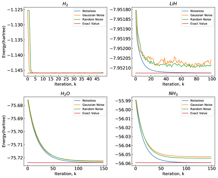
Figure 5: (a), (b), (c) and (d) show the gradient descent iteration process for convergence of ground state energy of H₂, LiH, H₂O and NH₃ respectively. The qubit Hamiltonians of the four molecules are obtained by STO-6G basis, which is more accurate than STO-3G basis.

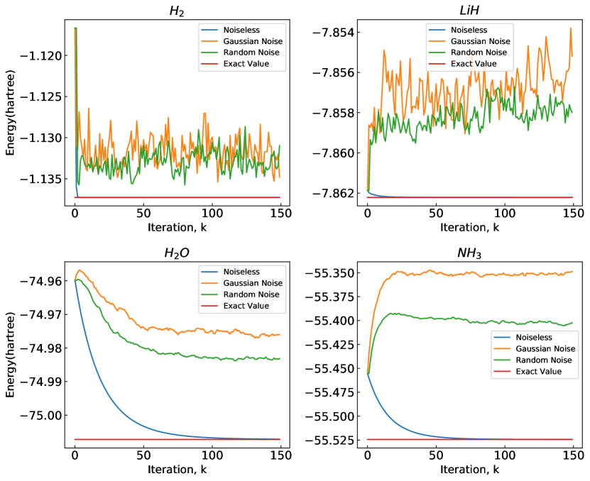
Figure 6: Infulence of large noise on FQE in (a) H₂, (b) LiH, (c) H₂O and (d) NH₃ molecules respectively. The amplitude of the random noise is 0.1 and the Gaussian noise parameters are $\mu=0,\sigma=0.1/3$.

V.3 Performance of FQE with large noise

We show the performance of FQE in large noise situations. As shown in Fig.6, when random noise becomes large, FQE will not converge to the ground state. Sometimes, it converges to exited energy-levels, such as in H₂O and NH₃. In some other situations, FQE behaves in a oscillation manner, such as in H₂ and LiH.

References

- (1) Paul Benioff. The computer as a physical system: A microscopic quantum mechanical hamiltonian model of computers as represented by turing machines. Journal of Statistical Physics, 22(5):563–591, 1980.
- (2) Ivanovich Manin. Vychislimoe i nevychislimoe. Sov. Radio, 1980.
- (3) Richard P Feynman. Simulating physics with computers. International Journal of Theoretical Physics, 21(6):467–488, 1982.
- (4) Seth Lloyd. Universal quantum simulators. Science, 273(5278):1073–1078, 1996.
- (5) Daniel S Abrams and Seth Lloyd. Simulation of many-body fermi systems on a universal quantum computer. Physical Review Letters, 79(13):2586, 1997.
- (6) A Yu Kitaev. Quantum measurements and the abelian stabilizer problem. arXiv preprint quant-ph/9511026, 1995.
- (7) Alán Aspuru-Guzik, Anthony D Dutoi, Peter J Love, and Martin Head-Gordon. Simulated quantum computation of molecular energies. Science, 309(5741):1704–1707, 2005.
- (8) Ryan Babbush, Peter J Love, and Alán Aspuru-Guzik. Adiabatic quantum simulation of quantum chemistry. Scientific Reports, 4:6603, 2014.
- (9) Guan-Ru Feng, Yao Lu, Liang Hao, Fei-Hao Zhang, and Gui-Lu Long. Experimental simulation of quantum tunneling in small systems. Scientific Reports, 3:2232, 2013.
- (10) Yao Lu, Guan-Ru Feng, Yan-Song Li, and Gui-Lu Long. Experimental digital quantum simulation of temporal–spatial dynamics of interacting fermion system. Science Bulletin, 60(2):241–248, 2015.
- (11) Ryan Babbush, Jarrod McClean, Dave Wecker, Alán Aspuru-Guzik, and Nathan Wiebe. Chemical basis of trotter-suzuki errors in quantum chemistry simulation. Physical Review A, 91(2):022311, 2015.
- (12) Shi-Jie Wei, Dong Ruan, and Gui-Lu Long. Duality quantum algorithm efficiently simulates open quantum systems. Scientific Reports, 6:30727, 2016.
- (13) Ryan Babbush, Dominic W Berry, Ian D Kivlichan, Annie Y Wei, Peter J Love, and Alán Aspuru-Guzik. Exponentially more precise quantum simulation of fermions in second quantization. New Journal of Physics, 18(3):033032, 2016.
- (14) Ryan Babbush, Dominic W Berry, Yuval R Sanders, Ian D Kivlichan, Artur Scherer, Annie Y Wei, Peter J Love, and Alán Aspuru-Guzik. Exponentially more precise quantum simulation of fermions in the configuration interaction representation. Quantum Science and Technology, 3(1):015006, 2017.
- (15) Ivan Kassal, Stephen P Jordan, Peter J Love, Masoud Mohseni, and Alán Aspuru-Guzik. Polynomial-time quantum algorithm for the simulation of chemical dynamics. Proceedings of the National Academy of Sciences, 105(48):18681–18686, 2008.
- (16) Ian D Kivlichan, Nathan Wiebe, Ryan Babbush, and Alán Aspuru-Guzik. Bounding the costs of quantum simulation of many-body physics in real space. Journal of Physics A: Mathematical and Theoretical, 50(30):305301, 2017.
- (17) Borzu Toloui and Peter J Love. Quantum algorithms for quantum chemistry based on the sparsity of the ci-matrix. arXiv preprint arXiv:1312.2579, 2013.
- (18) Alberto Peruzzo, Jarrod McClean, Peter Shadbolt, Man-Hong Yung, Xiao-Qi Zhou, Peter J Love, Alán Aspuru-Guzik, and Jeremy L O’brien. A variational eigenvalue solver on a photonic quantum processor. Nature Communications, 5:4213, 2014.
- (19) Jarrod R McClean, Jonathan Romero, Ryan Babbush, and Alán Aspuru-Guzik. The theory of variational hybrid quantum-classical algorithms. New Journal of Physics, 18(2):023023, 2016.
- (20) Jarrod R McClean, Ryan Babbush, Peter J Love, and Alán Aspuru-Guzik. Exploiting locality in quantum computation for quantum chemistry. The journal of Physical Chemistry Letters, 5(24):4368–4380, 2014.
- (21) James D Whitfield, Jacob Biamonte, and Alán Aspuru-Guzik. Simulation of electronic structure hamiltonians using quantum computers. Molecular Physics, 109(5):735–750, 2011.
- (22) Dave Wecker, Matthew B Hastings, and Matthias Troyer. Progress towards practical quantum variational algorithms. Physical Review A, 92(4):042303, 2015.
- (23) Matthew B Hastings, Dave Wecker, Bela Bauer, and Matthias Troyer. Improving quantum algorithms for quantum chemistry. Quantum Information & Computation, 15(1-2):1–21, 2015.
- (24) Oleksandr Kyriienko. Quantum inverse iteration algorithm for near-term quantum devices. arXiv preprint arXiv:1901.09988, 2019.
- (25) Pascual Jordan and Eugene P Wigner. About the pauli exclusion principle. Z. Phys., 47:631–651, 1928.
- (26) Sergey B Bravyi and Alexei Yu Kitaev. Fermionic quantum computation. Annals of Physics, 298(1):210–226, 2002.
- (27) Jacob T Seeley, Martin J Richard, and Peter J Love. The bravyi-kitaev transformation for quantum computation of electronic structure. The Journal of Chemical Physics, 137(22):224109, 2012.
- (28) Andrew Tranter, Sarah Sofia, Jake Seeley, Michael Kaicher, Jarrod McClean, Ryan Babbush, Peter V Coveney, Florian Mintert, Frank Wilhelm, and Peter J Love. The bravyi-kitaev transformation: Properties and applications. International Journal of Quantum Chemistry, 115(19):1431–1441, 2015.
- (29) Sergey Bravyi, Jay M Gambetta, Antonio Mezzacapo, and Kristan Temme. Tapering off qubits to simulate fermionic hamiltonians. arXiv preprint arXiv:1701.08213, 2017.
- (30) Ryan Babbush, Nathan Wiebe, Jarrod McClean, James McClain, Hartmut Neven, and Garnet Kin-Lic Chan. Low-depth quantum simulation of materials. Physical Review X, 8(1):011044, 2018.
- (31) M-H Yung, Jorge Casanova, Antonio Mezzacapo, Jarrod Mcclean, Lucas Lamata, Alan Aspuru-Guzik, and Enrique Solano. From transistor to trapped-ion computers for quantum chemistry. Scientific Reports, 4:3589, 2014.
- (32) Jiangfeng Du, Nanyang Xu, Xinhua Peng, Pengfei Wang, Sanfeng Wu, and Dawei Lu. Nmr implementation of a molecular hydrogen quantum simulation with adiabatic state preparation. Physical Review Letters, 104(3):030502, 2010.
- (33) Zhaokai Li, Xiaomei Liu, Hefeng Wang, Sahel Ashhab, Jiangyu Cui, Hongwei Chen, Xinhua Peng, and Jiangfeng Du. Quantum simulation of resonant transitions for solving the eigenproblem of an effective water hamiltonian. Physical Review Letters, 122(9):090504, 2019.
- (34) Pedram Roushan, Charles Neill, Anthony Megrant, Yu Chen, Ryan Babbush, Rami Barends, Brooks Campbell, Zijun Chen, Ben Chiaro, Andrew Dunsworth, et al. Chiral ground-state currents of interacting photons in a synthetic magnetic field. Nature Physics, 13(2):146, 2017.
- (35) Benjamin P Lanyon, James D Whitfield, Geoff G Gillett, Michael E Goggin, Marcelo P Almeida, Ivan Kassal, Jacob D Biamonte, Masoud Mohseni, Ben J Powell, Marco Barbieri, et al. Towards quantum chemistry on a quantum computer. Nature Chemistry, 2(2):106, 2010.
- (36) Stefano Paesani, Andreas A Gentile, Raffaele Santagati, Jianwei Wang, Nathan Wiebe, David P Tew, Jeremy L O’Brien, and Mark G Thompson. Experimental bayesian quantum phase estimation on a silicon photonic chip. Physical Review Letters, 118(10):100503, 2017.
- (37) Ya Wang, Florian Dolde, Jacob Biamonte, Ryan Babbush, Ville Bergholm, Sen Yang, Ingmar Jakobi, Philipp Neumann, Alán Aspuru-Guzik, James D Whitfield, et al. Quantum simulation of helium hydride cation in a solid-state spin register. ACS nano, 9(8):7769–7774, 2015.
- (38) Yangchao Shen, Xiang Zhang, Shuaining Zhang, Jing-Ning Zhang, Man-Hong Yung, and Kihwan Kim. Quantum implementation of the unitary coupled cluster for simulating molecular electronic structure. Physical Review A, 95(2):020501, 2017.
- (39) Cornelius Hempel, Christine Maier, Jonathan Romero, Jarrod McClean, Thomas Monz, Heng Shen, Petar Jurcevic, Ben P Lanyon, Peter Love, Ryan Babbush, et al. Quantum chemistry calculations on a trapped-ion quantum simulator. Physical Review X, 8(3):031022, 2018.
- (40) Peter JJ O’Malley, Ryan Babbush, Ian D Kivlichan, Jonathan Romero, Jarrod R McClean, Rami Barends, Julian Kelly, Pedram Roushan, Andrew Tranter, Nan Ding, et al. Scalable quantum simulation of molecular energies. Physical Review X, 6(3):031007, 2016.
- (41) Abhinav Kandala, Antonio Mezzacapo, Kristan Temme, Maika Takita, Markus Brink, Jerry M Chow, and Jay M Gambetta. Hardware-efficient variational quantum eigensolver for small molecules and quantum magnets. Nature, 549(7671):242, 2017.
- (42) Marc Ganzhorn, Daniel J Egger, P Barkoutsos, Pauline Ollitrault, Gian Salis, Nikolaj Moll, M Roth, A Fuhrer, P Mueller, S Woerner, et al. Gate-efficient simulation of molecular eigenstates on a quantum computer. Physical Review Applied, 11(4):044092, 2019.
- (43) Masoud Mohseni, Peter Read, Hartmut Neven, Sergio Boixo, Vasil Denchev, Ryan Babbush, Austin Fowler, Vadim Smelyanskiy, and John Martinis. Commercialize quantum technologies in five years. Nature News, 543(7644):171, 2017.
- (44) Leonie Mueck. Quantum reform. Nature Chemistry, 7(5):361, 2015.
- (45) Long Gui-Lu. General quantum interference principle and duality computer. Communications in Theoretical Physics, 45(5):825, 2006.
- (46) Stan Gudder. Mathematical theory of duality quantum computers. Quantum Information Processing, 6(1):37–48, 2007.
- (47) LONG Gui-Lu and Liu Yang. Duality computing in quantum computers. Communications in Theoretical Physics, 50(6):1303, 2008.
- (48) Long Gui-Lu, Liu Yang, and Wang Chuan. Allowable generalized quantum gates. Communications in Theoretical Physics, 51(1):65, 2009.
- (49) Gui Lu Long. Duality quantum computing and duality quantum information processing. International Journal of Theoretical Physics, 50(4):1305–1318, 2011.
- (50) Andrew M Childs and Nathan Wiebe. Hamiltonian simulation using linear combinations of unitary operations. arXiv preprint arXiv:1202.5822, 2012.
- (51) Dominic W Berry, Andrew M Childs, Richard Cleve, Robin Kothari, and Rolando D Somma. Simulating hamiltonian dynamics with a truncated taylor series. Physical Review Letters, 114(9):090502, 2015.
- (52) Shi-Jie Wei and Gui-Lu Long. Duality quantum computer and the efficient quantum simulations. Quantum Information Processing, 15(3):1189–1212, 2016.
- (53) HuaiXin Cao, Li Li, ZhengLi Chen, Ye Zhang, and ZhiHua Guo. Restricted allowable generalized quantum gates. Chinese Science Bulletin, 55(20):2122–2125, 2010.
- (54) Gui-Lu Long and Yang Sun. Efficient scheme for initializing a quantum register with an arbitrary superposed state. Physical Review A, 64(1):014303, 2001.
- (55) Patrick Rebentrost, Maria Schuld, Leonard Wossnig, Francesco Petruccione, and Seth Lloyd. Quantum gradient descent and newton’s method for constrained polynomial optimization. New Journal of Physics, 21(7):073023, 2019.
- (56) Tao Xin, Shi-Jie Wei, Julen S Pedernales, Enrique Solano, and Gui-Lu Long. Quantum simulation of quantum channels in nuclear magnetic resonance. Physical Review A, 96(6):062303, 2017.
- (57) Shi-Jie Wei, Tao Xin, and Gui-Lu Long. Efficient universal quantum channel simulation in ibm’s cloud quantum computer. SCIENCE CHINA Physics, Mechanics & Astronomy, 61(7):70311, 2018.
- (58) Maysum Panju. Iterative methods for computing eigenvalues and eigenvectors. arXiv preprint arXiv:1105.1185, 2011.