The ${\gamma^{*}\gamma^{*}\to\eta_{c}(1S,2S)}$ transition form factors for spacelike photons

Abstract

We derive the light-front wave function (LFWF) representation of the $\gamma^{*}\gamma^{*}\to\eta_{c}(1S)\,,\eta_{c}(2S)$ transition form factor $F(Q_{1}^{2},Q_{2}^{2})$ for two virtual photons in the initial state. For the LFWF, we use different models obtained from the solution of the Schrödinger equation for a variety of $c\bar{c}$ potentials. We compare our results to the BaBar experimental data for the $\eta_{c}(1S)$ transition form factor, for one real and one virtual photon. We observe that the onset of the asymptotic behaviour is strongly delayed and discuss applicability of the collinear and/or massless limit. We present some examples of two-dimensional distributions for $F(Q_{1}^{2},Q_{2}^{2})$. A factorization breaking measure is proposed and factorization breaking effects are quantified and shown to be almost model independent. Factorization is shown to be strongly broken, and a scaling of the form factor as a function of $\bar{Q}^{2}=(Q_{1}^{2}+Q_{2}^{2})/2$ is obtained.

I Introduction

The description of the hadronic structure in terms of the quark and gluon degrees of freedom is one of the main goals of the Quantum Chromodynamics (QCD). During the last years, our understanding about the partonic distributions has been substantially improved by the experimental data obtained in $ep$ and $pp$ colliders. Complementary information about the internal structure of mesons can be accessed by the study of the electromagnetic form factors and the meson - photon transition form factors. There has been a lot of interest recently in the exclusive production of mesons via photon fusion processes studied mainly at the $e^{+}e^{-}$ colliders Chernyak:2014wra . Such studies are strongly motivated by the expectation that at large photon virtualities the measurements of the cross sections will provide strong constrains in the probability amplitude for finding partons in the mesons Radyushkin:1977gp ; Lepage:1979zb ; Chernyak:1983ej . The meson - photon transition form factors are also of interest because of the role they play in the hadronic light-by-light contribution to the muon anomalous magnetic moment Jegerlehner:2017gek .

During the last years, a lot of attention has been paid to the case of pseudoscalar light meson - photon transition form factors Kroll:2010bf ; Stefanis:2014yha , mainly motivated by the experimental data from the CLEO, BaBar, Belle and L3 Collaborations for the $\pi^{0}$, $\eta$ and $\eta^{\prime}$ production in $e^{+}e^{-}$ collisions. These collaborations have extracted the transition form factor from single - tag events where only one of the leptons in the final state is measured. In this case, one of the photons is far off the mass shell, while the other is almost real. Such data have allowed to test the collinear factorization approach and the onset of the asymptotic regime, as well motivated the improvement of the theoretical approaches. Similar results have been obtained for the $\eta_{c}$ production. In this case, the $\eta_{c}$ mass provides a hard scale that justifies to use a perturbative approach even for zero virtualities. In the past this transition form factor has been studied in different approaches, (although often only for one virtual photon), such as: perturbative QCD Feldmann:1997te ; Cao:1997hw , lattice QCD DE2006 ; CLQCD , non-relativistic QCD FJS2015 ; WWSB2018 , QCD sum rules LM2012 , as well as from Dyson-Schwinger and Bethe-Salpeter equations CDCL2017 . In the light-front quark model (LFQM) the case of one virtual and one real photon has been studied in GL2013 ; Ryu:2018egt .

In the present paper we will treat the heavy meson - photon transition form factor, focusing our analysis on the pseudoscalar charmonium state $\eta_{c}(1S)$ and its radial excitation $\eta_{c}(2S)$. Here we will focus on calculating transition form factor for both virtual photons, which was not studied so far in the light-front approach. These double virtual transition form factors can be measured in $e^{+}e^{-}$ collisions in the double - tag mode, where both electron and positron are detected in the final state. Recent results for the $\eta^{\prime}$ production by the BaBar Collaboration BaBar:2018zpn have demonstrated that this study is feasible. Our study is motivated by the possibility of an accurate measurement of the double virtual transition form factors considering the high luminosity expected at Belle2. This may open new possibilities, the issue of factorization breaking of the transition form factors, which will be addressed in this paper. Regarding the wave functions of the quarkonia, we wish to use also $c\bar{c}$ wave functions obtained from realistic potential models. Here we will make use of the solutions obtained in CNKP2019 . We shall investigate how well they can describe the recent BaBar data Lees:2010de for $\gamma\gamma^{*}\to\eta_{c}(1S)$. We shall also calculate transition form factors for $\gamma\gamma^{*}\to\eta_{c}(2S)$, not yet measured, but could be considered for Belle 2 program.

The paper is organized as follows. In Section II, we present the light-front formalism that is used for computations of the $\gamma^{*}\gamma^{*}\to\eta_{c}$ form factor. Here, we provide the details of the light front $\eta_{c}(1S,2S)$ wave function calculations in the framework of the Schrödinger equation with a chosen set of $c\bar{c}$ interaction potentials, as well as derive the basic relations for the corresponding amplitude and the transition form factor. In Section III, we discuss the most relevant numerical results on the $\eta_{c}$ wave functions and the transition form factors for different $c\bar{c}$ potentials, which are also compared to the existing BaBar data for the $\eta_{c}(1S)$ state. Section IV summarizes the most important results of our analysis.

II The light-front formalism for the $\gamma^{*}\gamma^{*}\to\eta_{c}$ form factor

Our goal in this Section is to describe the $\gamma^{*}\gamma^{*}\rightarrow\eta_{c}$ form factor, which can be measured in $e^{+}e^{-}$ collisions using two - photon events in which both photons are far off the mass shell. The typical diagram is represented in Fig. 1. We will consider the light - front formalism, which allows to describe the meson in terms of the quark degrees of freedom. Let us first start from general kinematical considerations.

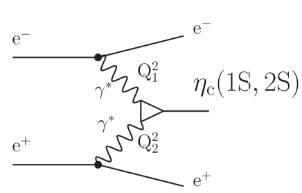
Figure 1: The $\eta_{c}$ production by the interaction of two virtual photons in $e^{+}e^{-}$ collisions.

The amplitude for the photon fusion $\gamma^{*}\gamma^{*}\to\eta_{c}$ has the general form dictated by the $J^{PC}=0^{-+}$ quantum numbers of the $\eta_{c}$:

$${\cal M}_{\mu\nu}(\gamma^{*}(q_{1})\gamma^{*}(q_{2})\to\eta_{c})=4\pi\alpha_{\rm em}\,(-i)\varepsilon_{\mu\nu\alpha\beta}q_{1}^{\alpha}q_{2}^{\beta}\,F(Q_{1}^{2},Q_{2}^{2})\,.$$ (1)

Here $Q_{i}^{2}=-q_{i}^{2}\geq 0,i=1,2$ are the virtualities of photons, which we take both to be space-like. The form factor $F(Q_{1}^{2},Q_{2}^{2})$ above is the object of interest in this paper. It is normalized such that the two-photon decay-width of the meson is obtained from

$$\Gamma(\eta_{c}\to\gamma\gamma)={\pi\over 4}\alpha^{2}_{\rm em}M_{\eta_{c}}^{3}\,|F(0,0)|^{2}\,.$$ (2)

For further calculation it is useful to choose a frame in which incoming photon four-momenta have the form

$$q_{1} = q_{1}^{+}n^{+}+q_{1\perp}\,,q_{2}=q_{2}^{-}n^{-}+q_{2\perp}\,.$$ (3)

Here

$$n^{\pm}={1\over\sqrt{2}}\,(1,0,0,\pm 1)\,,$$ (4)

and we will denote the transverse vectors by boldface vectors, e.g.

$$q_{i\perp}=(0,\mbox{\boldmath$q$}_{i},0)\,,\quad q_{i\perp}^{2}=-\mbox{\boldmath$q$}_{i}^{2}\,.$$ (5)

As the polarization vectors of off-shell photons we will choose $n^{+}$ and $n^{-}$ for the first and second photon, respectively. The four-momenta of photons satisfy $n^{+}\cdot q_{1}=n^{-}\cdot q_{2}=0$ We finally note that the transverse momentum of the meson is $\mbox{\boldmath$P$}=\mbox{\boldmath$q$}_{1}+\mbox{\boldmath$q$}_{2}$, and the photon light-front momenta fulfill

$$2q_{1}^{+}q_{2}^{-}=M_{\eta_{c}}^{2}+\mbox{\boldmath$P$}^{2}\,.$$ (6)

Projected onto the photon polarizations, the amplitude takes the simple form

$$n^{+\mu}n^{-\nu}{\cal M}_{\mu\nu}(\gamma^{*}(q_{1})\gamma^{*}(q_{2})\to\eta_{c})=4\pi\alpha_{\rm em}\,(-i)[\mbox{\boldmath$q$}_{1},\mbox{\boldmath$q$}_{2}]\,F(Q_{1}^{2},Q_{2}^{2})\,,$$ (7)

where $[\mbox{\boldmath$q$}_{1},\mbox{\boldmath$q$}_{2}]=q_{1}^{x}q_{2}^{y}-q_{1}^{y}q_{2}^{x}$.

II.1 Light front wave function of $\eta_{c}$

We treat the $\eta_{c}$ as a bound state of a charm quark and antiquark, thus assuming that the dominant contribution comes from the $c\bar{c}$ component in the Fock-state expansion:

$$|{\eta_{c};P_{+},\mbox{\boldmath$P$}}\rangle=\sum_{i,j,\lambda,\bar{\lambda}}{\delta^{i}_{j}\over\sqrt{N_{c}}}\,\int{dzd^{2}\mbox{\boldmath$k$}\over z(1-z)16\pi^{3}}\Psi_{\lambda\bar{\lambda}}(z,\mbox{\boldmath$k$})|{c_{i\lambda}(zP_{+},\mbox{\boldmath$p$}_{c})\bar{c}^{j}_{\bar{\lambda}}((1-z)P_{+},\mbox{\boldmath$p$}_{\bar{c}})}\rangle+\dots$$

Here the $c$-quark and $\bar{c}$-antiquark carry a fraction $z$ and $1-z$ respectively of the $\eta_{c}$’s plus-momentum. The light-front helicites of quark and antiquark are denoted by $\lambda,\bar{\lambda}$, and take values $\pm 1$. The transverse momenta of quark and antiquark are

$$\mbox{\boldmath$p$}_{c}=\mbox{\boldmath$k$}+z\mbox{\boldmath$P$}\,,\quad\mbox{\boldmath$p$}_{\bar{c}}=-\mbox{\boldmath$k$}+(1-z)\mbox{\boldmath$P$}\,.$$ (9)

The contribution of higher Fock states is expected to be suppressed at large $Q^{2}$. Moreover, the fact that non - relativistic potential models are able to describe the quarkonia properties implies that the valence $c\bar{c}$ Fock state probability of $\eta_{c}$ is almost 1 (see e.g. Feldmann:1997te , Feldmann:1998sh ). In Ref. GL2013 , the authors have assumed the $\eta_{c}$ wave function is a combination of the $u\bar{u}$, $d\bar{d}$, $s\bar{s}$ and $c\bar{c}$ Fock states. The resulting predictions for the $\eta_{c}$ form factor become dependent on the assumptions for the mixing angles, but are similar to those obtained assuming that the $\eta_{c}$ is a pure $c\bar{c}$ state. Therefore, our assumption for the $\eta_{c}$ wave function as a pure $c\bar{c}$ state is a very good approximation. The light-front wave function encodes all the necessary information on the bound state. Recently there has been a lot of interest in calculating light-front wave functions of heavy quarkonia, see for example Glazek:2006cu ; Gutsche:2014oua ; Li:2017mlw . Here we follow a different approach which relies on a prescription due to Terentev Terentev:1976jk , valid for weakly bound non-relativistic systems, which expresses the light-front wave function in terms of the rest-frame Schrödinger wave function.

In the ${}^{2S+1}L_{J}=^{1}S_{0}$ state the wave function of the two-body system for canonical spin-projections $\sigma\bar{\sigma}$ of quark and antiquark has the form

$$\Psi_{\sigma\bar{\sigma}}({\vec{p}})={1\over\sqrt{2}}\chi^{\dagger}_{\sigma}i\sigma_{2}\chi_{\bar{\sigma}}\,\,\phi(p)\,Y_{00}\Big{(}{\vec{p}\over p}\Big{)}\,={1\over\sqrt{2}}\chi^{\dagger}_{\sigma}i\sigma_{2}\chi_{\bar{\sigma}}\,\,{u(p)\over p}\,{1\over\sqrt{4\pi}}\,.$$ (10)

Here $\chi^{\dagger},\chi$ are the Pauli spinors, and $p=|\vec{p}|$. The normalization condition reads

$$\int d^{3}\vec{p}\sum_{\sigma\bar{\sigma}}|\Psi_{\sigma\bar{\sigma}}({\vec{p}})|^{2}=1\,,\,\int_{0}^{\infty}dp\,u^{2}(p)=1\,.$$ (11)

In order to apply Terentev’s transformation, we first introduce the relative momentum $\vec{p}$ of quark and antiquark in the center - of - mass frame at fixed invariant mass $M_{c\bar{c}}$,

$$\mbox{\boldmath$p$}=\mbox{\boldmath$k$},\quad p_{z}=(z-{1\over 2})M_{c\bar{c}}\,,$$ (12)

so that

$$\vec{p}^{2}={1\over 4}(M^{2}_{c\bar{c}}-4m_{c}^{2})={1\over 4}\Big{(}{\mbox{\boldmath$k$}^{2}+m_{c}^{2}\over z(1-z)}-4m_{c}^{2}\Big{)}\,.$$ (13)

We then decompose the helicity dependent light-front wave function (LFWF) into a spin/momentum and radial part as

$$\Psi_{\lambda\bar{\lambda}}(z,\mbox{\boldmath$k$})={\Gamma_{\lambda\bar{\lambda}}(z,\mbox{\boldmath$k$})\over{\cal N}(z,\mbox{\boldmath$k$})}\,\phi(z,\mbox{\boldmath$k$})\,.$$ (14)

To obtain the helicity dependent part of the LFWF one needs to transform the rest-frame spinors to the light-front spinors, which is effected by means of a Melosh transform Melosh:1974cu . This has been done e.g. in Ref. Jaus:1989au , and the the helicity-dependent vertex reads

$$\Gamma_{\lambda\bar{\lambda}}(z,\mbox{\boldmath$k$}) = \bar{u}_{\lambda}(zP_{+},\mbox{\boldmath$k$})\gamma_{5}v_{\bar{\lambda}}((1-z)P_{+},-\mbox{\boldmath$k$})$$ (15)

$$= {1\over\sqrt{z(1-z)}}\,\Big{\{}\lambda m_{c}\delta_{\lambda-\bar{\lambda}}-\lambda\sqrt{2}\mbox{\boldmath$k$}\cdot\mbox{\boldmath$e$}(-\lambda)\delta_{\lambda\bar{\lambda}}\Big{\}}\,,$$

where $\mbox{\boldmath$e$}(\lambda)=-(\lambda\mbox{\boldmath$e$}_{x}+i\mbox{\boldmath$e$}_{y})/\sqrt{2}$. The normalizing function ${\cal N}$ is

$${\cal N}(z,\mbox{\boldmath$k$})=\Big{(}\sum_{\lambda\bar{\lambda}}\Gamma_{\lambda\bar{\lambda}}(z,\mbox{\boldmath$k$})\Gamma^{*}_{\lambda\bar{\lambda}}(z,\mbox{\boldmath$k$})\Big{)}^{1/2}=\sqrt{2}\,\sqrt{{\mbox{\boldmath$k$}^{2}+m_{c}^{2}\over z(1-z)}}=\sqrt{2}M_{c\bar{c}}.$$ (16)

Then, if we take the meson state to obey the canonical relativistic normalization

$$\langle{\eta_{c};P_{+}^{\prime},\mbox{\boldmath$P$}^{\prime}}|{\eta_{c};P_{+},\mbox{\boldmath$P$}}\rangle=2P_{+}(2\pi)^{3}\delta(P_{+}^{\prime}-P_{+})\delta^{(2)}(\mbox{\boldmath$P$}^{\prime}-\mbox{\boldmath$P$}),$$ (17)

the radial light-front wave function $\phi(z,\mbox{\boldmath$k$})$ will be normalized as

$$\int_{0}^{1}{dz\over z(1-z)}\int{d^{2}\mbox{\boldmath$k$}\over 16\pi^{3}}\,|\phi(z,\mbox{\boldmath$k$})|^{2}=N_{c\bar{c}}=1\,.$$ (18)

To relate the radial LFWF to the rest-frame wave function, we should still take into account a jacobian from changing the integration measure

$${dzd^{2}\mbox{\boldmath$k$}\over z(1-z)}=4{d^{3}\vec{p}\over M_{c\bar{c}}}\,,$$ (19)

so that we obtain the identification

$$\phi(z,\mbox{\boldmath$k$})=\pi\sqrt{M_{c\bar{c}}}\,{u(p)\over p}\,.$$ (20)

To lighten up the notation of the amplitude, we also use

$$\psi(z,\mbox{\boldmath$k$})={\phi(z,\mbox{\boldmath$k$})\over{\cal N}(z,\mbox{\boldmath$k$})}={\pi\over\sqrt{2M_{c\bar{c}}}}{u(p)\over p}\,,$$ (21)

which we also refer to as the radial wave function.

Let us now present the details of computation of the radial wave function by means of the Schödinger equation with a set of chosen $c\bar{c}$ interaction potentials. For reviews on these topics, see e.g. Refs. Eichten:2007qx ; Voloshin:2007dx .

II.2 Schrödinger equation and $c\bar{c}$ interaction potentials

The charmonium wave function is found in the quark-antiquark rest frame by solving the Schrödinger equation which for the radial wave function $\psi(r)$ can be written as (for more details see Appendix in Ref. CNKP2019 )

$$\frac{\partial^{2}u(r)}{\partial r^{2}}=(V_{\rm eff}(r)-\epsilon)u(r)\,,\qquad u(r)=\sqrt{4\pi}\,r\psi(r)\,,\qquad\int\limits_{0}^{\infty}|u(r)|^{2}dr=1\,,$$ (22)

where

$$V_{\rm eff}(r)=m_{c}V(r)+\frac{l(l+1)}{r^{2}}\,,\qquad\epsilon=m_{c}\,E\,,$$ (23)

in terms of the interaction $c\bar{c}$ potential, $V(r)$. Here, we briefly describe several models for $V(r)$ chosen for our analysis.

• Harmonic oscillator:

  $$V(r)=\frac{1}{2}\,m_{c}\,\omega^{2}\,r^{2}\,,$$ (24)

  where for charmonia we adopt

  $$\omega=\frac{1}{2}(M_{2S}-M_{1S})\simeq 0.3\,{\rm GeV}\,,\qquad m_{c}=1.4\,{\rm GeV}\,.$$ (25)

  For such a simple choice of the interaction potential one finds an analytic solution of the Schrödinger equation (22)

  $$u(r)=\exp\biggl{[}-\frac{1}{4}\,m_{c}\,\omega\,r^{2}\biggr{]}\,,$$ (26)

  yielding a Gaussian shape of the wave function.

• Cornell potential Eichten:1978tg ; Eichten:1979ms :

  $$V(r)=-\frac{k}{r}+\frac{r}{a^{2}}\,,\quad k=0.52\,,\quad a=2.34\,\mathrm{GeV}^{-1}\,,$$ (27)

  and the charm quark mass is fixed to $m_{c}=1.84$ GeV.

• Logarithmic potential Quigg:1977dd :

  $$V(r)=-0.6635\,{\rm GeV}+(0.733\,{\rm GeV})\,\log(r\cdot 1\,{\rm GeV})\,,$$ (28)

  with $m_{c}=1.5$ GeV.

• Effective power-law potential Martin:1980jx ; Martin:1980xh :

  $$V(r)=-6.41\,{\rm GeV}+(6.08\,{\rm GeV})\,(r\cdot 1\,{\rm GeV})^{0.106}\,,$$ (29)

  assumes $m_{c}=1.334$ GeV Barik:1980ai .

• Buchmüller-Tye (BT) potential Buchmuller:1980su :

  $$V(r)=\begin{cases}\frac{k}{r}-\frac{8\pi}{27}\frac{v(\lambda r)}{r}\,,&r\geq 0.01\,{\rm fm}\\ -\frac{16\pi}{25}\frac{1}{r\,\ln w(r)}\Big{(}1+2\Big{(}\gamma_{E}+\frac{53}{75}\Big{)}\frac{1}{\ln w(r)}-\frac{462}{625}\,\,\frac{\ln\ln w(r)}{\ln w(r)}\Big{)}\,,&r<0.01\,{\rm fm}\,,\end{cases}$$ (30)

  where $\gamma_{E}=0.5772$ is the Euler constant, and the function $v(x)$ is known numerically from Ref. Buchmuller:1980su , and

  $$w(r)=\frac{1}{\lambda^{2}_{\rm MS}\,r^{2}}\,,\quad\lambda_{\rm MS}=0.509\,{\rm GeV}\,,\quad k=0.153\,{\rm GeV}^{2}\,,\quad\lambda=0.406\,{\rm GeV}\,.$$ (31)

  Here, the charm quark mass is taken to be $m_{c}=1.48\,{\rm GeV}$. One notices that the BT potential at small $r$ has a Coulomb-like behaviour, while at large $r$ – a string-like behaviour such that its difference from the Cornell potential is mainly at small $r$.

II.3 Light-front representation of the amplitude and transition form factor

Our calculation follows the standard procedure of perturbative QCD for exclusive processes. We regard the $\gamma^{*}\gamma^{*}\to c\bar{c}$ transition as a hard, perturbatively calculable process and convolute the amplitude with the bound state wave-function. We will assume later, that the charm quark mass $m_{c}$ by itself is large enough to justify perturbation theory and apply our results even in the limit of vanishing photon virtualities. Following Lepage:1980fj (see Eq. (A7) therein), the photon fusion amplitude can be expressed as

$${\cal M}_{\mu\nu}(\gamma^{*}(q_{1})\gamma^{*}(q_{2})\to\eta_{c}) = {{\rm Tr}\,\openone_{\rm color}\over\sqrt{N_{c}}}\int{dzd^{2}\mbox{\boldmath$k$}\over z(1-z)16\pi^{3}}$$

$$\times \sum_{\lambda\bar{\lambda}}\Psi^{*}_{\lambda\bar{\lambda}}(z,\mbox{\boldmath$k$}){\cal M}_{\mu\nu}(\gamma^{*}(q_{1})\gamma^{*}(q_{2})\to c_{\lambda}(z,\mbox{\boldmath$p$}_{c})\bar{c}_{\bar{\lambda}}(1-z,\mbox{\boldmath$p$}_{\bar{c}}))\,.$$

Here

$${\cal M}_{\mu\nu}(\gamma^{*}(q_{1})\gamma^{*}(q_{2})\to c_{\lambda}(z,\mbox{\boldmath$p$}_{c})\bar{c}_{\bar{\lambda}}(1-z,\mbox{\boldmath$p$}_{\bar{c}}))=4\pi\alpha_{\rm em}$$

$$\bar{u}_{\lambda}(zP_{+},\mbox{\boldmath$p$}_{c})\Big{(}\gamma_{\mu}{\hat{p}_{c}-\hat{q}_{1}-m_{c}\over t-m_{c}^{2}}\gamma_{\nu}+\gamma_{\nu}{\hat{p}_{c}-\hat{q}_{2}-m_{c}\over u-m_{c}^{2}}\gamma_{\mu}\Big{)}v_{\bar{\lambda}}((1-z)P_{+},\mbox{\boldmath$p$}_{\bar{c}}),$$ (33)

with $\hat{p}\equiv p^{\mu}\gamma_{\mu}$, is the standard Feynman amplitude including the $t$-channel and $u$-channel exchange of a quark. We can express the denominators of the propagators though LF-variables:

$$u-m_{c}^{2} = -{1\over 1-z}[\mbox{\boldmath$l$}_{A}^{2}+\mu^{2}]$$

$$t-m_{c}^{2} = -{1\over z}[\mbox{\boldmath$l$}_{B}^{2}+\mu^{2}].$$ (34)

Here we introduced the notation

$$\mbox{\boldmath$l$}_{A} = \mbox{\boldmath$p$}_{\bar{c}}-(1-z)\mbox{\boldmath$q$}_{1}=-\mbox{\boldmath$k$}+(1-z)\mbox{\boldmath$q$}_{2},$$

$$\mbox{\boldmath$l$}_{B} = \mbox{\boldmath$p$}_{c}-z\mbox{\boldmath$q$}_{1}=\mbox{\boldmath$k$}+z\mbox{\boldmath$q$}_{2},$$ (35)

and

$$\mu^{2}=z(1-z)\mbox{\boldmath$q$}_{1}^{2}+m_{c}^{2}\,.$$ (36)

Contracting the Feynman amplitude with $n_{\mu}^{+}n_{\nu}^{-}$ allows us to reduce the amplitude to a form where only simple spinor products of the form $\bar{u}\hat{n}^{+}v,\bar{u}\hat{n}^{-}u,\bar{v}\hat{n}^{-}v$ need to be performed. Using the spinors from Ref. Lepage:1980fj , we obtain then

$$n^{+\mu}n^{-\nu}{\cal M}_{\mu\nu}(\gamma^{*}(q_{1})\gamma^{*}(q_{2})\to\eta_{c})=4\pi\alpha_{\rm em}{{\rm Tr}\,\openone_{\rm color}\over\sqrt{N_{c}}}(-2)\int{dzd^{2}\mbox{\boldmath$k$}\over\sqrt{z(1-z)}16\pi^{3}}$$

$$\Big{\{}\Big{[}{1\over\mbox{\boldmath$l$}_{A}^{2}+\mu^{2}}-{1\over\mbox{\boldmath$l$}_{B}^{2}+\mu^{2}}\Big{]}\Big{[}i[\mbox{\boldmath$k$},\mbox{\boldmath$q$}_{1}]\Big{(}\Psi^{*}_{+-}(z,\mbox{\boldmath$k$})-\Psi^{*}_{-+}(z,\mbox{\boldmath$k$})\Big{)}$$

$$-\sqrt{2}m\Big{(}(\mbox{\boldmath$e$}(-)\mbox{\boldmath$q$}_{1})\Psi_{++}^{*}(z,\mbox{\boldmath$k$})+(\mbox{\boldmath$e$}(+)\mbox{\boldmath$q$}_{1})\Psi_{--}^{*}(z,\mbox{\boldmath$k$})\Big{)}\Big{]}$$

$$+\Big{[}{1-z\over\mbox{\boldmath$l$}_{A}^{2}+\mu^{2}}+{z\over\mbox{\boldmath$l$}_{B}^{2}+\mu^{2}}\Big{]}i[\mbox{\boldmath$q$}_{1},\mbox{\boldmath$q$}_{2}]\Big{(}\Psi^{*}_{+-}(z,\mbox{\boldmath$k$})-\Psi^{*}_{-+}(z,\mbox{\boldmath$k$})\Big{)}\Big{\}}\,.$$

Here, subscripts $\pm$ of the wave functions stand for helicities $\pm{1\over 2}$ of (anti-)quarks. Inserting the explicit expressions for the helicity dependent wave functions given in Eq. (15), we observe that there is a large cancellation between the parallel and antiparallel helicity configurations, and only the last term $\propto[\mbox{\boldmath$q$}_{1},\mbox{\boldmath$q$}_{2}]$ survives. It is then straightforward to read off our result for the $\gamma^{*}\gamma^{*}\to\eta_{c}$ form factor by comparing to Eq. (7):

$$F(Q_{1}^{2},Q_{2}^{2})=e_{c}^{2}\sqrt{N_{c}}\,4m_{c} \cdot \int{dzd^{2}\mbox{\boldmath$k$}\over z(1-z)16\pi^{3}}\psi(z,\mbox{\boldmath$k$})\Big{\{}{1-z\over(\mbox{\boldmath$k$}-(1-z)\mbox{\boldmath$q$}_{2})^{2}+z(1-z)\mbox{\boldmath$q$}_{1}^{2}+m_{c}^{2}}$$ (38)

$$+ {z\over(\mbox{\boldmath$k$}+z\mbox{\boldmath$q$}_{2})^{2}+z(1-z)\mbox{\boldmath$q$}_{1}^{2}+m_{c}^{2}}\Big{\}}\,.$$

and then to perform the integration over the azimuthal angle of $k$. Using

$$\int_{0}^{2\pi}{d\phi\over 2\pi}{1\over A+B\cos\phi}={1\over\sqrt{A^{2}-B^{2}}},$$ (39)

we can obtain

$$F(Q_{1}^{2},Q_{2}^{2})=e_{c}^{2}\sqrt{N_{c}}\,4m_{c} \cdot \int{dzkdk\over z(1-z)8\pi^{2}}\psi(z,\mbox{\boldmath$k$})$$

$$\Big{\{}{1-z\over\sqrt{(\mbox{\boldmath$k$}^{2}-m_{c}^{2}-z(1-z)\mbox{\boldmath$q$}_{1}^{2}-(1-z)^{2}\mbox{\boldmath$q$}_{2}^{2})^{2}+4\mbox{\boldmath$k$}^{2}(m_{c}^{2}+z(1-z)\mbox{\boldmath$q$}_{1}^{2})}}$$

$$+{z\over\sqrt{(\mbox{\boldmath$k$}^{2}-m_{c}^{2}-z(1-z)\mbox{\boldmath$q$}_{1}^{2}-z^{2}\mbox{\boldmath$q$}_{2}^{2})^{2}+4\mbox{\boldmath$k$}^{2}(m_{c}^{2}+z(1-z)\mbox{\boldmath$q$}_{1}^{2})}}\Big{\}}.$$

This form puts into evidence, that the invariant form factor $F(Q_{1}^{2},Q_{2}^{2})$ is a function of $Q_{1}^{2}=\mbox{\boldmath$q$}_{1}^{2}$ and $Q_{2}^{2}=\mbox{\boldmath$q$}_{2}^{2}$ only. Notice that by the Bose-symmetry, the form factor must be a symmetric function of $Q_{1}^{2},Q_{2}^{2}$. This is evidently not obvious from the representations Eq. (38) or Eq. (LABEL:eq:FF2), as the integrand is manifestly asymmetric in $\mbox{\boldmath$q$}_{1},\mbox{\boldmath$q$}_{2}$. However, as will be demonstrated below by the numerical results, our representation has the required symmetry. In particular, in the limit of one on-shell photon, one must have, that $F(Q^{2})\equiv F(Q^{2},0)=F(0,Q^{2})$, and the two different integral representations for $F(Q^{2})$ which follow from Eq. (38) coincide with the ones found in Ref. Ryu:2018egt , where their equivalence was also demonstrated numerically.

A number of limits of Eq. (38) are interesting. Firstly, the value $F(0,0)$ for two on-shell photons is related to the two-photon decay width by Eq. (2). First note, that

$$F(0,0)=e_{c}^{2}\sqrt{N_{c}}\,4m_{c}\cdot\int{dzd^{2}\mbox{\boldmath$k$}\over z(1-z)16\pi^{3}}{\psi(z,\mbox{\boldmath$k$})\over\mbox{\boldmath$k$}^{2}+m_{c}^{2}}\,.$$ (41)

Let us write this result as an integral over the three-momentum $\vec{p}$ and the radial wave function $u(p)$.

$$F(0,0) = e_{c}^{2}\sqrt{N_{c}}4m_{c}\int{4d^{3}\vec{p}\over{M_{c\bar{c}}}16\pi^{3}}\,{\psi(z,\mbox{\boldmath$k$})\over\mbox{\boldmath$k$}^{2}+m_{c}^{2}}$$ (42)

$$= e_{c}^{2}\sqrt{2N_{c}}{m_{c}\over\pi}\int_{0}^{\infty}{dp\,p\,u(p)\over\sqrt{M_{c\bar{c}}^{3}}(p^{2}+m_{c}^{2})}\int_{-1}^{1}{d\cos\theta\over 1-\beta^{2}\cos^{2}\theta}$$

$$= e_{c}^{2}\sqrt{2N_{c}}\,{2m_{c}\over\pi}\,\int_{0}^{\infty}{dp\,p\,u(p)\over\sqrt{M_{c\bar{c}}^{3}}(p^{2}+m_{c}^{2})}\,{1\over 2\beta}\log\left({1+\beta\over 1-\beta}\right)\,,$$

Here we used, that in polar coordinates $\mbox{\boldmath$k$}^{2}=p^{2}\sin^{2}\theta$, hence $\mbox{\boldmath$k$}^{2}+m_{c}^{2}=(p^{2}+m_{c}^{2})(1-\beta^{2}\cos^{2}\theta)$, where we introduced

$$\beta={p\over\sqrt{p^{2}+m_{c}^{2}}}\quad,$$ (43)

the velocity $v/c$ of the quark in the $c\bar{c}$ cms-frame. Similar results for the relativistic corrections to the decay width exist in the literature, see e.g. Ref. Ebert:2003mu and references therein. Notice that in these approaches typically the running of the mass $M_{c\bar{c}}$ with $p$ is neglected.

In the non-relativistic (NR) limit, where $p^{2}/m_{c}^{2}\ll 1,\beta\ll 1$, the invariant mass $M_{c\bar{c}}$ approaches $M_{c\bar{c}}=2m_{c}$. If we neglect the binding energy, and identify $2m_{c}=M_{\eta_{c}}$, we obtain

$$F(0,0) = e_{c}^{2}\sqrt{N_{c}}\sqrt{2}{4\over\pi\sqrt{M_{\eta_{c}}^{5}}}\int_{0}^{\infty}dp\,p\,u(p)=e_{c}^{2}\sqrt{N_{c}}{4\,R(0)\over\sqrt{\pi M_{\eta_{c}}^{5}}}\,\,.$$ (44)

Here $R(0)$ is the value of the radial wave function $R(r)=u(r)/r$ at the origin. This yields the well known result for the $\gamma\gamma$-width (see e.g. Table 2.2 in Ref. Novikov:1977dq )

$$\Gamma(\eta_{c}\to\gamma\gamma) = {4\alpha_{\rm em}^{2}e_{c}^{4}N_{c}\over M_{\eta_{c}}^{2}}|R(0)|^{2}\,,$$ (45)

which serves as a check on our normalization. In the same limit, which amounts to an expansion around $\mbox{\boldmath$k$}=0$ and $z=1/2$ in Eq. (38), we can derive the transition form factor in the NRQCD-limit,

$$F(Q_{1}^{2},Q_{2}^{2})=e_{c}^{2}\sqrt{N_{c}}{4\over\sqrt{\pi M_{\eta_{c}}}}{1\over Q_{1}^{2}+Q_{2}^{2}+M_{\eta_{c}}^{2}}\,R(0)\,.$$ (46)

Still another interesting limit exists, namely at very large $Q_{i}^{2}$, the $k$-smearing becomes unimportant, and one can neglect $k$ in the hard matrix element of Eq. (38). Then only the LFWF appears under the $k$ integral, and the hard scattering factorization in terms of the distribution amplitude emerges. We introduce the distribution amplitude (DA) at a scale $\mu_{0}^{2}$ as

$$f_{\eta_{c}}\,\varphi(z,\mu_{0}^{2}) = {1\over z(1-z)}{\sqrt{N_{c}}\,4m_{c}\over 16\pi^{3}}\int d^{2}\mbox{\boldmath$k$}\,\theta(\mu_{0}^{2}-\mbox{\boldmath$k$}^{2})\,\psi(z,\mbox{\boldmath$k$})\,.$$ (47)

The DA is conveniently normalized as

$$\int_{0}^{1}dz\,\varphi(z,\mu_{0}^{2})=1,$$ (48)

so that we can extract the so-called decay constant $f_{\eta_{c}}$ from the integral over $z$ in Eq. (47). The transition form factor simplifies to

$$F(Q_{1}^{2},Q_{2}^{2})=e_{c}^{2}\,f_{\eta_{c}}\, \cdot \int_{0}^{1}dz\Big{\{}{(1-z)\,\varphi(z,\mu_{0}^{2})\over(1-z)^{2}Q_{1}^{2}+z(1-z)Q_{2}^{2}+m_{c}^{2}}$$ (49)

$$+ {z\,\varphi(z,\mu_{0}^{2})\over z^{2}Q_{1}^{2}+z(1-z)Q_{2}^{2}+m_{c}^{2}}\,\Big{\}}\,.$$

This representation is valid in the limit of large photon virtualities $Q_{1}^{2},Q_{2}^{2}$.

III Numerical results

In this Section we will present our results for the doubly virtual transition form factor, which will be calculated for the different models for the meson wave function. A comparison with the current experimental data will be presented and the onset of the asymptotic regime will be discussed. Moreover, in order to estimate the factorization breaking in the transition form factor we will also estimate the normalized form factor, defined by:

$${\tilde{F}}(Q_{1}^{2},Q_{2}^{2})=\frac{F(Q_{1}^{2},Q_{2}^{2})}{F(0,0)}\;,$$ (50)

which nicely quantifies the deviation from point-like coupling. A popular model for the transition form factor is based on the vector meson dominance approach (see e.g. Ref. Lees:2010de ), and reads

$${\tilde{F}}(Q_{1}^{2},Q_{2}^{2})=\frac{M_{J/\Psi}^{2}}{Q_{1}^{2}+M_{J/\Psi}^{2}}\cdot\frac{M_{J/\Psi}^{2}}{Q_{2}^{2}+M_{J/\Psi}^{2}}\;.$$ (51)

It features a factorized dependence on the photon virtualities, which we expect to be broken. In our analysis, we will quantify the factorization breaking of the transition form factor by estimating the quantity defined by:

$$R(Q_{1}^{2},Q_{2}^{2})=\frac{{\tilde{F}}(Q_{1}^{2},Q_{2}^{2})}{{\tilde{F}}(Q_{1}^{2},0){\tilde{F}}(0,Q_{2}^{2})}\;.$$ (52)

III.1 $c\bar{c}$ wave functions of $\eta_{c}(1S)$ and $\eta_{c}(2S)$

Our wave functions $u(p)$ were obtained by Fourier transform from the $r$-dependent $c\bar{c}$ wave functions obtained as a solution of the Schrödinger equation with different, realistic, potentials from the literature as described in the previous Section. In Fig. 2 we show the wave function $u(p)$ for different potentials for the $1S$ state (left panel) and for the $2S$ radial excitation (right panel). We have that the different models predict similar shapes for the wave functions, but differ in its predictions for the position of the peaks and the approach to the large momentum limit.

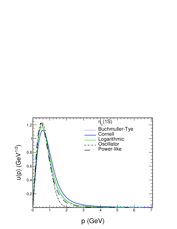
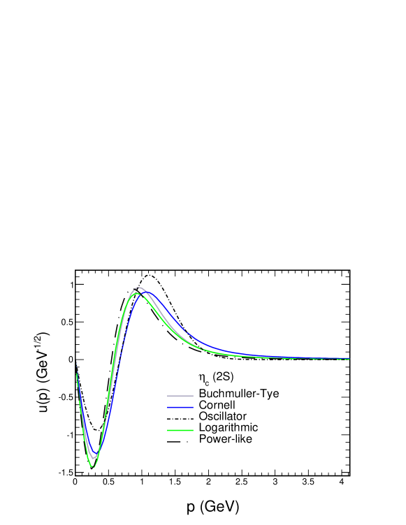
Figure 2: Momentum space wave function $u(p)$ for $\eta_{c}(1S)$ (upper panel) and $\eta_{c}(2S)$ (lower panel) for different potentials.

Using the Terentev prescription (see Eq. (12)) we obtain wave functions in the light-front variables $z$ and $k_{T}=|\mbox{\boldmath$k$}|$. In Fig. 3 we show as an example the light-front wave function of Eq. (21) in the $(z,k_{T})$-space for the Buchmüller-Tye potential. As expected, the wave function is strongly peaked at $z\approx 1/2$ and is strongly suppressed in the endpoints. These properties are shared by all wave functions for the potentials used by us. The Cornell potential wave function somewhat stands out as it has the hardest tail at large momenta.

III.2 $\gamma^{*}\gamma^{*}$ transition form factor

We start the presentation of our results from the value of $F(0,0)$ for $\eta_{c}(1S)$ and $\eta_{c}(2S)$ obtained from the different potential model wave functions. The obtained results for $F(0,0)$, together with the resulting decay width into photons, $\Gamma_{\gamma\gamma}$ are collected in Table 1 for the $\eta_{c}(1S)$ and Table 2 for the $\eta_{c}(2S)$, respectively. Rather different results are obtained for different potentials, and they are not always consistent with the one obtained from radiative decay width $\Gamma_{\gamma\gamma}$, rather well known from recent experiments Tanabashi:2018oca . It is interesting to compare these –fully relativistic– results to the ones obtained from the wave function at the origin collected in Table 3 and Table 4 respectively for $\eta_{c}$ (1S) and $\eta_{c}$ (2S). We observe that the relativistic corrections are fairly strong, especially for the Cornell-potential.

Also shown in Tables 1 and 2 are the values for the so-called decay constant $f_{\eta_{c}}$. In the case of the $1S$ state, the agreement with a value extracted by the CLEO collaboration Edwards:2000bb is generally quite good. We wish to point out that the decay constant $f_{\eta_{c}}$ is not directly related to the two-photon decay width $\Gamma_{\gamma\gamma}$. Such a relation only exists in the non - relativistic limit, where both quantities are expressed in terms of the wave function at the origin.

In the upper panel of Fig. 4 we show our results for the normalized $\gamma^{*}\gamma\to\eta_{c}$ transition form factor ${\tilde{F}}(Q^{2},0)$ as a function of photon virtuality ($Q^{2}$) for different potential models. Below we will also use the notation $F(Q^{2})=F(Q^{2},0)=F(0,Q^{2})$, when one of the photons is on-shell. For reference we also show the BaBar experimental data Lees:2010de . The oscillator and power-law potentials give the best description of the BaBar data. This appears to be related to the lower value of $m_{c}$ used with these potentials. A modification of the quark mass to $m_{c}=1.3\,\textrm{GeV}$ in the hard matrix element in fact leads to a much better agreement with the BaBar data.

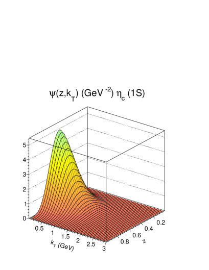
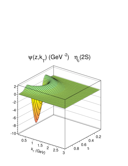
Figure 3: The light-front radial wave function $\psi(z,\mbox{\boldmath$k$})$ of Eq. (21) in the ($z,k_{T}$) space for Buchmüller-Tye potential for $\eta_{c}$(1S) and $\eta_{c}$(2S), respectively. Here $k_{T}=|\mbox{\boldmath$k$}|$.

Table 1: Transition form factor $|F(0,0)|$ for $\eta_{c}(1S)$ at $Q_{1}^{2}=Q_{2}^{2}=$0.

potential type	$m_{c}\,[\rm{GeV}$]	$|F(0,0)|\,[\rm{GeV}^{-1}]$	$\Gamma_{\gamma\gamma}$ [$\rm{keV}$]	$f_{\eta_{c}}[\textrm{GeV}]$
harmonic oscillator	1.4	0.051	2.89	0.2757
logarithmic	1.5	0.052	2.95	0.3373
power-like	1.334	0.059	3.87	0.3074
Cornell	1.84	0.039	1.69	0.3726
Buchmüller-Tye	1.48	0.052	2.95	0.3276
experiment	-	0.067 $\pm$ 0.003 Tanabashi:2018oca	5.1 $\pm$ 0.4 Tanabashi:2018oca	0.335 $\pm$ 0.075 Edwards:2000bb

Table 2: Transition form factor $|F(0,0)|$ for $\eta_{c}(2S)$ at $Q_{1}^{2}=Q_{2}^{2}=$0.

potential type	$m_{c}\,[\rm{GeV}$]	$|F(0,0)|\,[\rm{GeV}^{-1}]$	$\Gamma_{\gamma\gamma}$ [$\rm{keV}$]	$f_{\eta_{c}}[\textrm{GeV}]$
harmonic oscillator	1.4	0.03492	2.454	0.2530
logarithmic	1.5	0.02403	1.162	0.1970
power-like	1.334	0.02775	1.549	0.1851
Cornell	1.84	0.02159	0.938	0.2490
Buchmüller-Tye	1.48	0.02687	1.453	0.2149
experiment Tanabashi:2018oca	-	0.03266 $\pm$ 0.01209	2.147 $\pm$ 1.589

Table 3: R(0) and $\gamma\gamma$-width for $\eta_{c}$(1S) derived in the non-relativistic limit.

potential type	R(0)$[\textrm{GeV}^{3/2}]$	$\Gamma_{\gamma\gamma}$ [$\rm{keV}$] $\rm{M}=\rm{M}_{\eta_{c}}$	$\Gamma_{\gamma\gamma}$ [$\rm{keV}$] $\rm{M}=2m_{c}$
harmonic oscillator	0.6044	5.1848	5.8815
logarithmic	0.8919	11.290	11.157
power-like	0.7620	8.2412	10.297
Cornell	1.2065	20.660	13.568
Buchmüller-Tye	0.8899	11.240	11.409

Table 4: R(0) and $\gamma\gamma$-width for $\eta_{c}$(2S) derived in the non-relativistic limit.

potential type	R(0) $[\textrm{GeV}^{3/2}]$	$\Gamma_{\gamma\gamma}$ [$\rm{keV}$] $\rm{M}=\rm{M}_{\eta_{c}}$	$\Gamma_{\gamma\gamma}$ [$\rm{keV}$] $\rm{M}=2m_{c}$
harmonic oscillator	0.7402	5.2284	8.8214
logarithmic	0.6372	3.8745	5.6946
power-like	0.5699	3.0993	5.7594
Cornell	0.9633	8.8550	8.6493
Buchmüller-Tye	0.7185	4.9263	7.4374

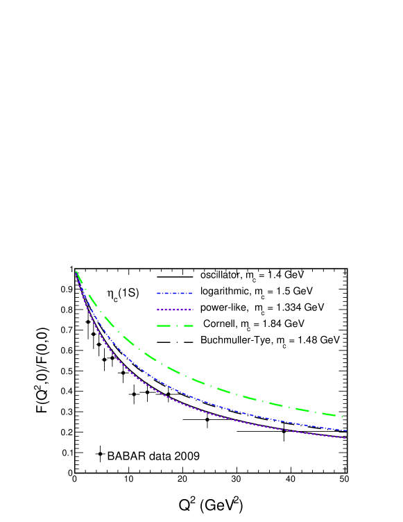
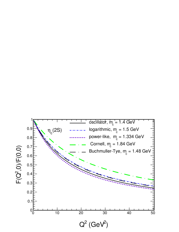
Figure 4: The dependence of the normalized transition form factor $\tilde{F}(Q^{2},0)$ on space-like photon virtuality for $\eta_{c}(1S)$ and $\eta_{c}(2S)$. For the case of the $\eta_{c}(1S)$, the BaBar experimental data Lees:2010de are shown for comparison.

The $\gamma^{*}\gamma$ transition form factor for the $\eta_{c}(2S)$ is shown in the lower panel of Fig. 4 . In this case the ${\tilde{F}}(Q^{2},0)={\tilde{F}}(0,Q^{2})$ has a somewhat harder tail as a function of $Q^{2}$ than for the $\eta_{c}(1S)$.

In Fig.5 we show the rate of approaching of $Q^{2}F(Q^{2})$ to its asymptotic value predicted by Brodsky and Lepage Lepage:1980fj . For the asymptotic distribution amplitude $\varphi(z,\mu^{2})=6z(1-z)$, one would obtain $Q^{2}F(Q^{2})=\frac{8}{3}f_{\eta_{c}}$. Therefore the horizontal lines $\frac{8}{3}f_{\eta_{c}}$ are shown for reference (upper panel - $\eta_{c}$(1S), lower panel - $\eta_{c}$(2S)), considering the values for $f_{\eta_{c}}$ presented in Tables 1 and 2. We do not observe approaching towards BL asymptotic value for $Q^{2}\leq 50$ GeV². While our results flatten out at large $Q^{2}$, their asymptotic value is much smaller then the one predicted within the hard scattering formalism.

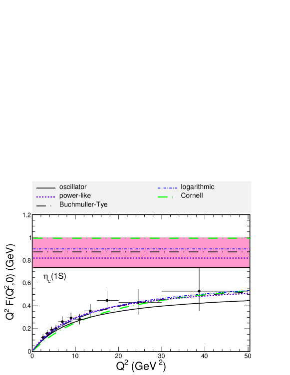
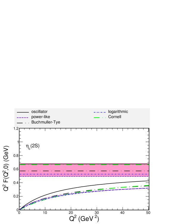
Figure 5: $Q^{2}F(Q^{2})$ as a function of photon virtuality for $\eta_{c}$(1S) (upper panel), $\eta_{c}(2S)$ (lower panel) for different potentials used in the present paper.

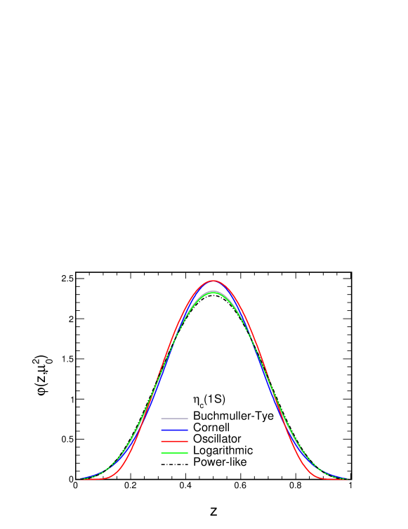
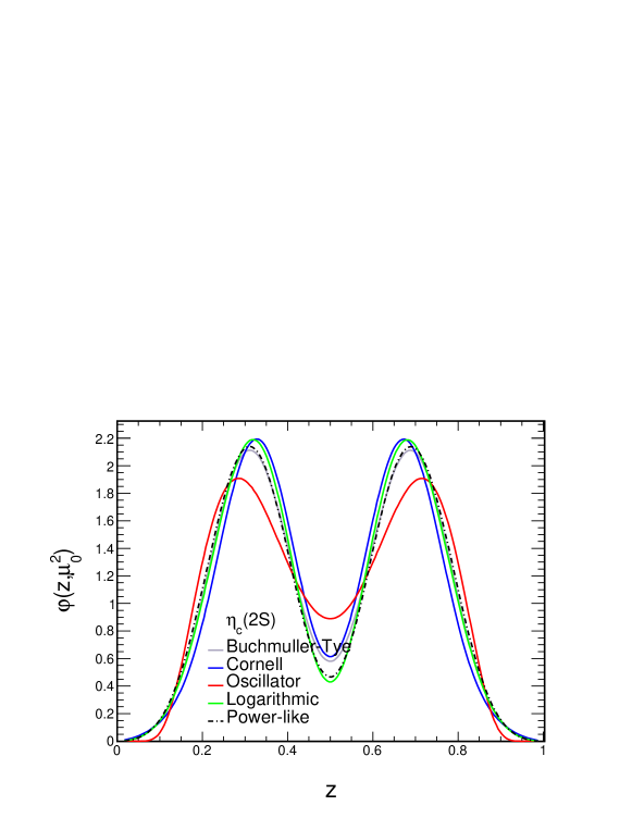
Figure 6: Distribution amplitudes for different wave functions for $\eta_{c}$ (1S) (upper panel) and for $\eta_{c}$ (2S) (lower panel).

In order to understand the results for $Q^{2}F(Q^{2})$ shown above, let us discuss the applicability of collinear approach, commonly used for light pseudoscalar mesons, for the $\eta_{c}$ case. From Eq. (49), one has that the collinear formula with the correct asymptotics reads:

$$F(Q^{2},0)=F(0,Q^{2})=e_{c}^{2}f_{\eta_{c}}\int_{0}^{1}dz\,\Big{\{}{z\,\varphi(z,\mu^{2})\over z^{2}Q^{2}+m_{c}^{2}}+{(1-z)\varphi(z,\mu^{2})\over(1-z)^{2}Q^{2}+m_{c}^{2}}\Big{\}}\;.$$ (53)

The evolution with the factorization scale is easily implemented in the formalism of distribution amplitudes. This is routinely done for light pseudoscalar mesons ($\pi^{0}\,,\eta\,,\eta^{\prime}$) see e.g. a recent NLO analysis KPK2019 . For $c\bar{c}$ (or $b\bar{b}$) quarkonia the situation is much more complicated and quark mass effects and/or higher twists must be included. In Fig. 6 we show the distribution amplitude at a factorization scale $\mu=3\,\rm{GeV}$ calculated from our wave functions for both $\eta_{c}$ (1S) and $\eta_{c}$ (2S). To perform the evolution with the hard scale, the distribution amplitude is expanded with the help of the Gegenbauer $C^{3/2}_{n}$ polynomials:

$$\varphi(z,\mu^{2})=6z(1-z)\left(1+a_{2}(\mu^{2})C_{2}^{3/2}(2z-1)+...\right)\;.$$ (54)

We extract the Gegenbauer coefficients by means of

$$a_{n}(\mu_{0})=\frac{2(2n+3)}{3(n+1)(n+2)}\cdot\int_{0}^{1}{dz\varphi(z,\mu_{0})C_{n}^{3/2}(2z-1)}\,.$$ (55)

They evolve according to

$$a_{n}(\mu) =a_{n}(\mu_{0})\cdot\left[\frac{\alpha_{s}(\mu)}{\alpha_{s}(\mu_{0})}\right]^{\gamma_{n}/\beta_{0}}\,,$$ (56)

with the the anomalous dimensions $\gamma_{n}$, which can be found for example in Ref. Lepage:1980fj .

For $\eta_{c}(1S)$, the $a_{2}$ coefficient dominates and is typically -0.3 at the initial evolution scale. For the $\eta_{c}(2S)$ the $n=4,6$ coefficients dominate. We show the Gegenbauer coefficients at the scale $\mu_{0}=3\,\rm GeV$ for both $\eta_{c}(1S)$ and $\eta_{c}(2S)$ in Table 5.

Table 5: Extracted coefficients $a_{n}(\mu_{0})$, for the Buchmüller-Tye potential

n	$a_{n}(\mu_{0})\;\eta_{c}(1S)$	$a_{n}(\mu_{0})\;\eta_{c}(2S)$
2	-0.284	-0.0765
4	0.0635	-0.1627
6	-0.008157	0.128
8	-0.000619	-0.049
10	0.000216	0.0088

In Fig. 7 we illustrate the effect of evolution on $Q^{2}F(Q^{2})$. We compare the result obtained with our original formula, given by Eq. (38). In addition, we show results obtained with the collinear formula (53) using distribution amplitudes obtained from our light-front wave functions (see Fig.6). There is only some difference at low $Q^{2}$. Finally we show also result obtained within collinear approach with QCD evolution of distribution amplitudes built in, starting from $\mu_{0}=3\,\rm GeV$. The effect of evolution is very weak. The reader is asked to notice much broader range of $Q^{2}$ in the figure compared to that in previous figures. Summarizing the effect of evolution can be safely neglected for $Q^{2}<$ 100 $GeV^{2}$, i.e. in the range of our interest, i.e. where $F(Q^{2})$ can be measured.

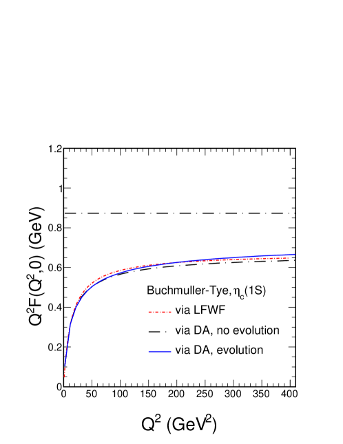
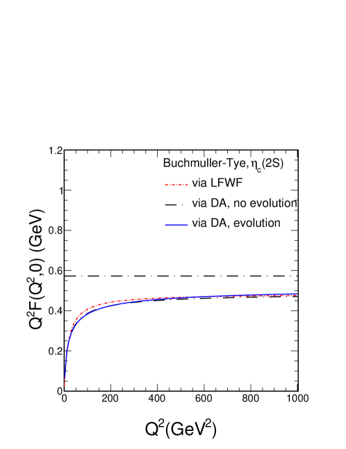
Figure 7: $Q^{2}F(Q^{2})$ for $\eta_{c}$ (1S)(upper panel) and $\eta_{c}$ (2S) (lower panel) as a function of photon virtuality. The horizontal line is the limit for $Q^{2}\rightarrow\infty$, calculated for the Buchmüller-Tye potential. The red dashed line (via LFWF) was obtained according to Eq. (38). The black dashed-dotted curve (via DA) and the blue solid curve (via DA, evolution) were calculated with Eq. (53) respectively with and without evolution of Gegenbauer coefficients $a_{n}$.

Now we wish to present also two-dimensional distributions for the $\gamma^{*}\gamma^{*}$ transition form factor as a function of the photon virtualities $Q_{1}^{2}$ and $Q_{2}^{2}$. As an example in Fig.8 we again show our results for the Buchmüller-Tye potential. To investigate the scaling properties, we show the transition form factor as a function of the variables

$$\omega=\frac{Q_{1}^{2}-Q_{2}^{2}}{Q_{1}^{2}+Q_{2}^{2}}\,\,\,\,\mbox{and}\,\,\,\bar{Q}^{2}=\frac{Q_{1}^{2}+Q_{2}^{2}}{2}\,.$$ (57)

One can see that $F$ (and $\widetilde{F}$) is almost independent of the asymmetry parameter $\omega$. For comparison $\gamma^{*}\gamma^{*}\to\pi^{0}$ transition the dependence on $\omega$ is somewhat stronger DKV2001 . Note that for the VDM model (51) some dependence on $\omega$ would be obtained. Future investigation of the slow $\omega$ dependence would be in our opinion an interesting task for Belle 2.

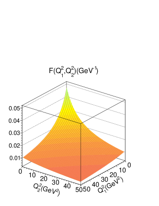
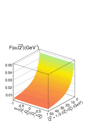
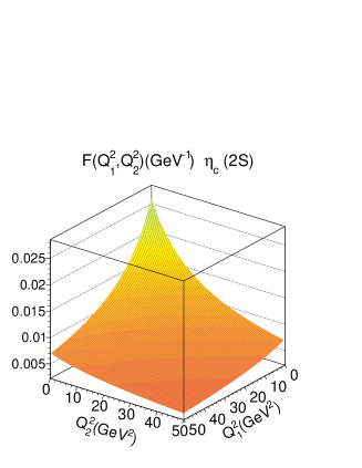
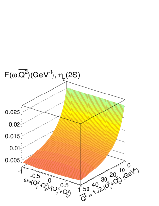
Figure 8: The $\gamma^{*}\gamma^{*}\rightarrow\eta_{c}$ (1S) (top panels) and $\gamma^{*}\gamma^{*}\rightarrow\eta_{c}$ (2S) (bottom panels) form factor as a function of ($Q_{1}^{2},Q_{2}^{2}$) and ($\omega,\bar{Q^{2}}$) for the Buchmüller-Tye potential for illustration, other potentials discussed in the present paper behave similarly.

In Fig. 9 we show deviations from the factorization breaking (see Eq. (52)), for the Buchmüller-Tye potential. We observe that $R(0,Q_{2}^{2})=R(Q_{1}^{2},0)=1$. The factorization breaking pattern looks very similar for different potentials (not shown explicitly here).

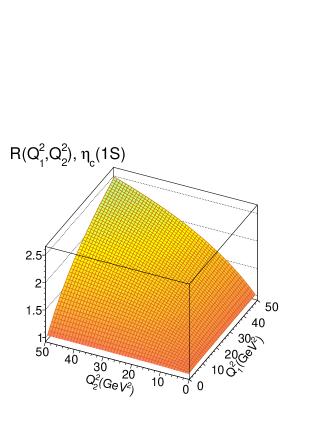
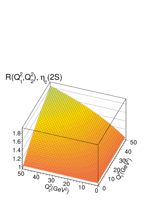
Figure 9: The deviations from the factorization breaking ($R$) as a function of ($Q_{1}^{2},Q_{2}^{2}$) for Buchmüller-Tye potential; left panel - $\eta_{c}$(1S), right panel - $\eta_{c}$(2S)).

IV Conclusions

The description of transition form factors is directly related to our understanding of the structure of bound states in QCD. In the present paper we have studied the transition form factors for $\gamma^{*}\gamma^{*}\to\eta_{c}$ (1S,2S) for two space-like virtual photons, which can be accessed experimentally in future measurements of the cross section for the $e^{+}e^{-}\rightarrow e^{+}e^{-}\eta_{c}$ process in the double - tag mode. The light-front wave function representation of these observables has been derived and discussed.

We have calculated the transition form factor for different wave functions obtained as a solution of the Schrödinger equation for the $c\bar{c}$ system for different phenomenological $c\bar{c}$ potentials from the literature. The rest-frame momentum space wave functions have been transformed to the light-front representation using the Terentev prescription. Firstly we have presented the transition form factor for only one off-shell photon as a function of its virtuality and compared to the BaBar data for the $\eta_{c}(1S)$ case. We have also presented the delayed convergence of the form factor to its asymptotic value $\frac{8}{3}f_{\eta_{c}}$ as predicted by the standard hard scattering formalism. Our results for $Q^{2}F(Q^{2})$ approach to a lower asymptotic value. The Brodsky-Lepage limit can only be obtained after including QCD evolution of the distribution amplitudes for massless quarks, but appears irrelevant in the accessible kinematic domain. We conclude that it is not necessary to include the QCD evolution for $Q^{2}<$ 100 GeV². This justifies, a posteriori, our results obtained within the approach using $c\bar{c}$ wave functions. Furthermore, we have presented two-dimensional distributions in the virtualities of photons of the $\gamma^{*}\gamma^{*}\eta_{c}$ transition form factor for $\eta_{c}(1S)$ and $\eta_{c}(2S)$. We have predicted a very slow dependence on the asymmetry parameter $\omega$, which could be verified experimentally at Belle 2. We have also defined a measure of factorization breaking and have calculated it for different potentials as a function of $(Q_{1}^{2},Q_{2}^{2})$. The results on the $Q_{1}^{2},Q_{2}^{2}$ dependence are almost model independent.

Finally, it is important to emphasize that the $\eta_{c}$ production in hadronic collisions is dominated, at lowest order, by the $g^{*}g^{*}\rightarrow\eta_{c}$ subprocess, which is identical (up to global color factors) to the $\gamma^{*}\gamma^{*}\rightarrow\eta_{c}$ amplitude derived in this paper. Consequently, our results can also be useful to estimate the $\eta_{c}$ production at the LHC, which is currently a theme of intense debate (see e.g. Refs. kniel_prl15 ; han_prl15 ; zhang_prl15 ).

V Acknowledgments

V.P.G. was partially financed by the Brazilian funding agencies CNPq, FAPERGS and INCT-FNA (project number 464898/2014-5). R.P. is supported in part by the Swedish Research Council grants, contract numbers 621-2013-4287 and 2016-05996, by CONICYT grant MEC80170112, as well as by the European Research Council (ERC) under the European Union’s Horizon 2020 research and innovation programme (grant agreement No 668679). This work was also supported in part by the Ministry of Education, Youth and Sports of the Czech Republic, project LT17018. The work has been performed in the framework of COST Action CA15213 “Theory of hot matter and relativistic heavy-ion collisions” (THOR).

References

- (1) V. L. Chernyak and S. I. Eidelman, Prog. Part. Nucl. Phys. 80, 1 (2014) [arXiv:1409.3348 [hep-ph]].
- (2) A. V. Radyushkin, JINR-P2-10717 (Dubna, 1977), [hep-ph/0410276]; A. V. Efremov and A. V. Radyushkin, Theor. Math. Phys. 42, 97 (1980) [Teor. Mat. Fiz. 42, 147 (1980)]; Phys. Lett. 94B, 245 (1980).
- (3) G. P. Lepage and S. J. Brodsky, Phys. Lett. 87B, 359 (1979).
- (4) V. L. Chernyak and A. R. Zhitnitsky, Phys. Rept. 112, 173 (1984).
- (5) F. Jegerlehner, Springer Tracts Mod. Phys. 274, pp.1 (2017).
- (6) P. Kroll, Eur. Phys. J. C 71, 1623 (2011) [arXiv:1012.3542 [hep-ph]].
- (7) N. G. Stefanis, S. V. Mikhailov and A. V. Pimikov, Few Body Syst. 56, no.6-9, 295 (2015). [arXiv:1411.0528 [hep-ph]].
- (8) T. Feldmann and P. Kroll, Phys. Lett. B 413, 410 (1997) [hep-ph/9709203].
- (9) T. Feldmann, P. Kroll and B. Stech, Phys. Lett. B 449, 339 (1999) doi:10.1016/S0370-2693(99)00085-4 [hep-ph/9812269].
- (10) F. g. Cao and T. Huang, Phys. Rev. D 59, 093004 (1999) [hep-ph/9711284].
- (11) J.J. Dudek and R.G. Edwards, Phys. Rev. Lett. 97, 172001 (2006).
- (12) T. Chen et al. (CLQCD collaboration), Eur. Phys. J. C 76, 358 (2016).
- (13) F. Feng, Y. Jia and W.-L. Sang, Phys. Rev. Lett. 115, 222001 (2015).
- (14) S.Q. Wang, X.G. Wu, W.-L. Sang and S.J. Brodsky, Phys. Rev. D97, 0094034 (2018).
- (15) W. Lucha and D. Melikhov, Phys. Rev. D86, 016001 (2012).
- (16) J. Chen, M. Ding, L. Chang and Y.-X. Liu, Phys. Rev. D 95. 016010 (2017).
- (17) C.Q. Geng and C.C. Lih, Eur. Phys. J C73, 2505 (2013).
- (18) H. Y. Ryu, H. M. Choi and C. R. Ji, Phys. Rev. D 98, no.3, 034018 (2018) [arXiv:1804.08287 [hep-ph]].
- (19) J. P. Lees et al. [BaBar Collaboration], Phys. Rev. D 98, no.11, 112002 (2018).
- (20) J. Cepila, J. Nemchik, M. Krelina and R. Pasechnik, arXiv:1901.02664 [hep-ph].
- (21) J. P. Lees et al. [BaBar Collaboration], Phys. Rev. D 81, 052010 (2010) [arXiv:1002.3000 [hep-ex]].
- (22) V. N. Gribov, Y. L. Dokshitzer and J. Nyiri, Camb. Monogr. Part. Phys. Nucl. Phys. Cosmol. 27 (2012).
- (23) S. D. Glazek and J. Mlynik, Phys. Rev. D 74, 105015 (2006) [hep-th/0606235].
- (24) T. Gutsche, V. E. Lyubovitskij, I. Schmidt and A. Vega, Phys. Rev. D 90, no.9, 096007 (2014) [arXiv:1410.3738 [hep-ph]].
- (25) Y. Li, P. Maris and J. P. Vary, Phys. Rev. D 96, no.1, 016022 (2017) [arXiv:1704.06968 [hep-ph]].
- (26) M. V. Terentev, Sov. J. Nucl. Phys. 24, 106 (1976) [Yad. Fiz. 24, 207 (1976)].
- (27) H.J. Melosh, Phys. Rev. D9, 1095 (1974).
- (28) W. Jaus, Phys. Rev. D 41, 3394 (1990).
- (29) E. Eichten, S. Godfrey, H. Mahlke and J. L. Rosner, Rev. Mod. Phys. 80, 1161 (2008) [hep-ph/0701208].
- (30) M. B. Voloshin, Prog. Part. Nucl. Phys. 61, 455 (2008) [arXiv:0711.4556 [hep-ph]].
- (31) E. Eichten, K. Gottfried, T. Kinoshita, K.D. Lane and T.M. Yan, Phys. Rev. D 21, 203 (1980).
- (32) E. Eichten, K. Gottfried, T. Kinoshita, K.D. Lane and T.M. Yan, Phys. Rev. D 17, 3090 (1978); Erratum: [Phys. Rev. D 21, 313 (1980)].
- (33) C. Quigg and J.L. Rosner, Phys. Lett. B 71, 153 (1977).
- (34) A. Martin, Phys. Lett. B 93, 338 (1980).
- (35) A. Martin, CERN-TH-2876, C80-03-09-25.
- (36) N. Barik and S.N. Jena, Phys. Lett. B 97, 265 (1980).
- (37) W. Buchmüller and S.H.H. Tye, Phys. Rev. D 24, 132 (1981).
- (38) G. P. Lepage and S. J. Brodsky, Phys. Rev. D 22, 2157 (1980).
- (39) D. Ebert, R. N. Faustov and V. O. Galkin, Mod. Phys. Lett. A 18, 601 (2003) [hep-ph/0302044].
- (40) V. A. Novikov, L. B. Okun, M. A. Shifman, A. I. Vainshtein, M. B. Voloshin and V. I. Zakharov, Phys. Rept. 41, 1 (1978).
- (41) M. Tanabashi et al. [Particle Data Group], Phys. Rev. D 98, no.3, 030001 (2018).
- (42) K. W. Edwards et al. [CLEO Collaboration], Phys. Rev. Lett. 86, 30 (2001) [hep-ex/0007012].
- (43) S. Ong, Phys. Rev. D 52, 3111 (1995).
- (44) M. Diehl, P. Kroll and C. Vogt, Eur. Phys. J. C 22, 430 (2001).
- (45) P. Kroll and K. Passek-Kumericki, Phys. Lett. B 793, 195 (2019) [arXiv:1903.06650 [hep-ph]].
- (46) M. Butenschoen, Z. G. He and B. A. Kniehl, Phys. Rev. Lett. 114, no. 9, 092004 (2015)
- (47) H. Han, Y. Q. Ma, C. Meng, H. S. Shao and K. T. Chao, Phys. Rev. Lett. 114, no.9, 092005 (2015)
- (48) H. F. Zhang, Z. Sun, W. L. Sang and R. Li, Phys. Rev. Lett. 114, no. 9, 092006 (2015)