The Physical Origin of the Venus Low Atmosphere Chemical Gradient

Abstract

Venus shares many similarities with the Earth, but concomitantly, some of its features are extremely original. This is especially true for its atmosphere, where high pressures and temperatures are found at the ground level. In these conditions, carbon dioxide, the main component of Venus’ atmosphere, is a supercritical fluid. The analysis of VeGa-2 probe data has revealed the high instability of the region located in the last few kilometers above the ground level. Recent works have suggested an explanation based on the existence of a vertical gradient of molecular nitrogen abundances, around $5$ ppm per meter. Our goal was then to identify which physical processes could lead to the establishment of this intriguing nitrogen gradient, in the deep atmosphere of Venus. Using an appropriate equation of state for the binary mixture CO₂–N₂ under supercritical conditions, and also molecular dynamics simulations, we have investigated the separation processes of N₂ and CO₂ in the Venusian context. Our results show that molecular diffusion is strongly inefficient, and potential phase separation is an unlikely mechanism. We have compared the quantity of CO₂ required to form the proposed gradient with what could be released by a diffuse degassing from a low volcanic activity. The needed fluxes of CO₂ are not so different from what can be measured over some terrestrial volcanic systems, suggesting a similar effect at work on Venus.

1. Introduction

Venus, sometimes considered as the “sister planet” of Earth, is actually very different than what titles implies. Essentially, Venus and the Earth share similar masses, densities, and heliocentric distances (Malcuit, 2015); other features differ significantly, and this is particularly the case for their atmospheres. For instance, at the ground level, the air of Venus is hellish: the temperature is close to $740$ K and the pressure is in the vicinity of $90$ bars. Because carbon dioxide dominates the atmospheric composition, with a mole fraction around $97$%, at low altitude, the Venusian air is a supercritical fluid. The second most abundant atmospheric compound is molecular nitrogen, with a mole fraction of about $3$%. Therefore, nitrogen is also in a supercritical state. In the phase diagram displayed in Fig. 1 we have plotted carbon dioxide and nitrogen’s critical points as well as the pressure ($P$)–temperature ($T$) atmospheric profile measured during the descent of the VeGa-2 probe (Lorenz et al., 2018). Venus is not the only celestial body harboring supercritical fluids. Giant planets Jupiter and Saturn, together with brown dwarfs and some exoplanets, have regions where molecular hydrogen is in the supercritical domain (Trachenko et al., 2014). In the case of terrestrial planets, supercritical fluids could be present, but less abundant. For example, on the Earth, supercritical water has been found in some hydrothermal vents (Koschinsky et al., 2008), and its presence was also known for a long time in geothermal reservoirs (Agostinetti et al., 2017). Additionally, high density and high temperature lead to efficient dissolving and extracting abilities of supercritical fluids, allowing many industrial applications (Bolmatov et al., 2013).
Recently, the existence of a gradient of chemical composition in the Venus deep atmosphere, i.e. for layers below the altitude of $\sim 7000$ m, has been suggested (Lebonnois & Schubert, 2017). The abundance of nitrogen seems to decrease from $\sim 3.5$% at $7000$m̃, to zero at ground level, yielding an average gradient of about $5$ ppm m^-1. If accepted as real, the proposed gradient may have two origins: (1) a N₂–CO₂ separation due to specific fluid features (to be identified, these can be categorized as “intrinsic” origins) and (2) phenomena related to Venus surface properties, such as the continuous release of some amount of carbon dioxide from the Venusian crust or molecular nitrogen entrapping, which can be referred as “extrinsic origins.” As a very first attempt, we have checked that the apparent composition gradient could not simply be an effect of the compressibility of the CO₂–N₂ mixture. For this purpose, we have employed an equation of state (EoS; Duan et al., 1996) specifically developed for mixtures like CO₂–N₂, under supercritical conditions. The compressibility factor (see for instance Zucker & Biblarz, 2002) $Z$ measures the deviation of real gas compressibility from an ideal behavior, and a value around unity shows a compressibility similar to that of an ideal gas. We found that the compressibility factor $Z$ stays around $1$ in the deep atmosphere of Venus. This result, also supported by laboratory measurements (Mohagheghian et al., 2015), has already been found by Lebonnois & Schubert (2017), and we confirm it.
Although the fluid under consideration here seems to exhibit typical compressibility properties, in Sec. 2 we discuss the possibility of a separation of N₂ and CO₂, induced by gravity, and facilitated by some potential properties of our supercritical mixture. In Sec. 3 we discuss the role of “extrinsic effects” like crust release of carbon dioxide, before concluding on a plausible scenario.

2. The Possible Separation of N₂ and CO₂ under Supercritical Conditions

2.1. The Effect of Molecular Diffusion

For almost a century, chemical composition variations have been known among terrestrial reservoirs of hydrocarbons, i.e., containing gases or petroleum (Sage & Lacey, 1939), or both. These variations are horizontal, i.e., the composition of the mixture changes from one well to another, but also vertical. In the latter case, for a given well, the abundances of species evolve with depth. The emergence of such a gradient of composition is due to the effect of gravity and to thermodiffusion. In this context, the convection is not very efficient because the fluid is trapped in a porous medium. A vast collection of literature is dedicated to this topic, and informative albeit not exhaustive reviews may be found elsewhere (Thomas, 2007; Obidi, 2014). Here, we focus our attention on the physics, based on molecular diffusion, of the vertical compositional grading. Our goal is to evaluate the efficiency of molecular diffusion under supercritical conditions. If the air mixing, due to atmospheric circulation, is slow or inefficient enough, the deep atmosphere of Venus could be the subject of analogous physical processes, leading to a gradient of nitrogen concentration. This assumption may also be regarded as an ideal or limiting case.
In a fluid medium undergoing a gradient of composition, temperature, or pressure, fluxes of matter appear. These transport mechanisms are ruled by the physics of irreversible physical processes. The best-known laws in this field are certainly the Fick’s law of molecular diffusion and its Fourier counterpart for thermal conduction.

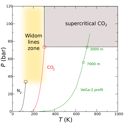
Figure 1.— Simplified phase diagram of CO₂: the position of the critical point of pure CO₂ has been plotted (red circle), together with the liquid-vapor equilibrium line (red line); the supercritical CO₂ regions are shaded gray. The pressure (in bars) is denoted $P$, while $T$ represents the temperature (in kelvins) of the system. Similarly, the N₂ critical point and liquid-vapor equilibrium line are shown in black. When some amount of molecular nitrogen is added to pure CO₂, the critical point of the mixture is shifted, leading to a position within the yellow-shaded zone (van Konynenburgand & Scott, 1980; Goos et al., 2011). For small fractions of N₂, the position of the critical point is shifted by a few bars and a few Kelvin (Goos et al., 2011). The green line refers to the pressure–temperature profile of Venus atmosphere derived from measurements performed by the VeGa-2 probe (Lorenz et al., 2018).

In the general case, the total diffusion mass flux $\overrightarrow{\jmath_{1}}$ (kg m^-2 s^-1) of one of the two components making a binary mixture may be written as (Bird et al., 1960; Ghorayeb & Firoozabadi, 2000)

$$\begin{split}\overrightarrow{\jmath_{1}}=-\rho&D_{12}\frac{M_{1}M_{2}}{\bar{M}^{2}}\,\left\{\left.\frac{\partial\mathrm{ln}\,f_{1}}{\partial\mathrm{ln}\,x_{1}}\right|_{P,T}\overrightarrow{\nabla}x_{1}\right.\\ &\left.+\frac{x_{1}}{RT}\left(\bar{V}_{1}-\frac{M_{1}}{\rho}\right)\overrightarrow{\nabla}P+\frac{k_{T\,1,2}}{T}\,\overrightarrow{\nabla}T\right\}\end{split}$$ (1)

with $\rho$ being the density (kg m^-3) of the mixture, $D_{12}$ being the Fickean diffusion coefficient (m² s^-1) of species ($1$) in ($2$), $M_{1}$ and $M_{2}$ are the respective molecular weights (kg mol^-1) of the involved species, and $\bar{M}$ is the average molecular weight of the system: $\bar{M}=x_{1}M_{1}+(1-x_{1})M_{2}$. The fugacity, which measures non-ideal effects for a real gas, is represented by $f_{1}$ for compound ($1$). Adopting a typical notation, $x_{1}$ and $\bar{V}_{1}$ are the mole fraction of species ($1$) and its molar volume (m³ mol^-1), and $P$ and $T$ are respectively the local pressure (Pa) and temperature (K). In the last term of Eq. (1), the thermal diffusion ratio $k_{T\,1,2}$ (dimensionless) is a function of $\alpha_{T\,1,2}$, the thermal diffusion coefficient (dimensionless), according to the formula $k_{T\,1,2}=\alpha_{T\,1,2}x_{1}(1-x_{1})$.
In the phenomenological Eq. (1), we recognize three terms that correspond to three different processes. The first term represents the well known molecular Fickean diffusion. The second term is for pressure diffusion, which may lead to gravity segregation. The last term represents thermal diffusion (called the Soret effect for liquids), which is the tendency for species of a convection-free mixture to separate under temperature gradient.

Using the pressure and temperature gradients, provided by the VeGa-2 probe (Lorenz et al., 2018) under steady-state conditions (i.e. $j_{1}=0$) to solve Eq. (1) allows the derivation of the chemical composition as a function of altitude $z$. In a first approach, if we assume the Venus deep atmosphere fluid acts like an ideal gas, the equation to be integrated is simply

$$\begin{split}\frac{\partial x_{1}}{\partial z}=-\frac{x_{1}}{P}&\left(1-\frac{M_{1}}{\bar{M}}\right)\left.\frac{\partial P}{\partial z}\right|_{\rm\tiny VeGa2}\\ &-\frac{\alpha_{T\,1,2}}{T}\,x_{1}(1-x_{1})\,\left.\frac{\partial T}{\partial z}\right|_{\rm\tiny VeGa2}\end{split}$$ (2)

In our approach, nitrogen is our chosen compound ($1$). We recall that, for a mixture of ideal gases, the fugacity is simply $f_{1}=x_{1}P$, leading to $(\partial\,\mathrm{ln}\,f_{1}/\partial\,\mathrm{ln}\,x_{1})=1$. The partial molar volume is, for all involved species, $RT/P$; and the density can be written as $\rho=P\bar{M}/RT$. Thanks to the kinetic theory of gases (Chapman & Cowling, 1970), the thermal diffusion coefficient $\alpha_{T\,1,2}$ may be estimated for the system N₂–CO₂. In the general case, $\alpha_{T\,1,2}$ may be positive or negative, depending on the respective masses of compounds of interest. For N₂–CO₂, using Chapman & Cowling’s approach, we found this coefficient to be negative. As a consequence, heavier molecules, i.e. CO₂, should gather in the coldest regions at high altitude. At the same time, the pressure term plays the opposite role, by enriching the highest layers in N₂. However, our numerical simulations show that thermal diffusion remains notably smaller than pressure diffusion, with thermal flux around $30$% of pressure flux.
By integrating Eq. (2) from the top of the Venus deep atmosphere, i.e. from an altitude of $7000$ m, down to the surface, we obtained a nitrogen mole fraction gradient of $\sim 0.6$ ppm m^-1. This value is roughly one order of magnitude lower than the expected gradient (Lebonnois & Schubert, 2017) of $\sim 5$ ppm m^-1.

Now we can turn to a more realistic model; taking into account non-ideal effects, the relevant equation is then (Ghorayeb & Firoozabadi, 2000)

$$\begin{split}\left.\frac{\partial\,\mathrm{ln}\,f_{1}}{\partial\,\mathrm{ln}\,x_{1}}\right|_{P,T}\frac{\partial x_{1}}{\partial z}&+\frac{x_{1}}{RT}\left(\bar{V}_{1}-\frac{M_{1}}{\rho}\right)\left.\frac{\partial P}{\partial z}\right|_{\rm\tiny VeGa2}\\ &+\frac{\alpha_{T\,1,2}}{T}\,x_{1}(1-x_{1})\,\left.\frac{\partial T}{\partial z}\right|_{\rm\tiny VeGa2}=0\end{split}$$ (3)

The pressure gradient can then be expressed as a function of density and Venus’ gravity $g_{V}$; we then get

$$\begin{split}\left.\frac{\partial\,\mathrm{ln}\,f_{1}}{\partial\,\mathrm{ln}\,x_{1}}\right|_{P,T}\frac{\partial x_{1}}{\partial z}=\frac{x_{1}}{RT}&\left(\bar{V}_{1}-\frac{M_{1}}{\rho}\right)\rho\,g_{V}\\ &-\frac{k_{T,12}}{T}\frac{\partial T}{\partial z}\end{split}$$ (4)

With this new equation, we can expect the enhanced composition gradient $\partial x_{1}/\partial z$. Indeed, one of the criteria (Myerson & Senol, 1984) used to determine the critical point position is $\partial\mu_{1}/\partial x_{1}=0$. This latter condition is essentially equivalent (Taylor & Krisna, 1993) to $\partial\mathrm{ln}f_{1}/\partial\mathrm{ln}\,x_{1}=0$. Then, in the supercritical region, when the representative point of the system approaches the critical point, this derivative tends to zero. At the same time, the quantity $\bar{V}_{1}-M_{1}/\rho$ generally has a non-zero finite value. As a consequence, the gradient $\partial x_{1}/\partial z$ could take very large values when the system is in the vicinity of the critical point. Of course, this property is unchanged if the thermodiffusion term is taken into account. In order to derive quantitative estimations we have employed the EoS (Duan et al., 1996) developed for the system CO₂–N₂ under supercritical conditions, and already used for our computations of the compressibility factor $Z$. The fugacity of nitrogen $f_{1}$, and its derivative, are obtained from the fugacity coefficient $\Phi_{1}=f_{1}/P_{1}$ provided by the EoS. Here, the quantity $P_{1}$ denotes the partial pressure of nitrogen: $P_{1}=x_{1}P$. The partial molar volume of N₂ comes from the equation (see the Appendix A. for derivation)

$$\bar{V}_{1}=\frac{RT}{P}\,\left(1+P\,\left.\frac{\partial\mathrm{ln}\Phi_{1}}{\partial P}\right|_{T,x_{1},x_{2}}\right)$$ (5)

We made comparisons, using the pressure–temperature profile acquired by VeGa-2, between quantities evaluated from the ideal gas EoS and those calculated with the help of the more advanced Duan’s EoS. Not surprisingly, we found negligible differences remaining below a few percent. Concerning the derivative of the fugacity, we consistently obtained values around unity. Our simulations have shown that $\partial\mathrm{ln}f_{1}/\partial\mathrm{ln}x_{1}$ tends to zero only in the close neighborhood of the binary mixture critical point. The Venusian atmosphere seems too far from this critical point to account for the effect expected for tiny values of $\partial\mathrm{ln}f_{1}/\partial\mathrm{ln}x_{1}$, i.e. a very large gradient of chemical composition. In summary, our equilibrium model, taking into account non-ideal effects, leads to a gradient similar to the value already obtained for an ideal gas, one order of magnitude lower than what it is needed to explain the observations.

Up to this point, we have left out the question of timescales. The equilibrium states described above need a certain amount of time to be reached by the system. Since the transport processes considered in our model rely mainly on molecular diffusion, it is quite easy to make a rough estimation of the associated timescale. If $H$ is the typical size of a system containing a fluid, the order of magnitude of the timescale $\tau_{\rm diff}$ associated to diffusion processes is given by $\tau_{\rm diff}\sim H^{2}/D$ where $D$ is the molecular diffusion coefficient. For the behavior of a solute, here nitrogen, dispersed in a volume of supercritical carbon dioxide, the value $D_{\rm N_{2}-CO_{2}}$ (m² s^-1) of this coefficient may be evaluated with the help of the Wilke–Chang equation (Wilke & Chang, 1955; Sassiat et al., 1987) which is essentially an empirical modification of the Stokes–Einstein relation

$$D_{\rm N_{2}-CO_{2}}\simeq 7.4\times 10^{-15}\frac{TM_{\rm CO_{2}}^{1/2}}{\eta_{\rm CO_{2}}V_{\rm N_{2},b}^{0.6}}$$ (6)

where $T$ is the temperature, the molecular weight of CO₂ is $M_{s}$ (44 g mol^-1), the viscosity of supercritical carbon dioxide is denoted $\eta_{\rm CO_{2}}$ (Pa s), while the molar volume of nitrogen at its boiling temperature, under atmospheric pressure, is represented by $V_{\rm N_{2},b}$. Here, we have $V_{\rm N_{2},b}\simeq 35$ cm³ mol^-1. The supercritical carbon dioxide viscosity $\eta_{\rm CO_{2}}$ may be estimated with the help of the Heidaryan et al.’s correlation (Heidaryan et al., 2011); for $T=700$ K and $P=100$ bar, we got $\eta_{\rm CO_{2}}\sim 3\times 10^{-5}$ Pa s. All in all, we obtained $D_{\rm N_{2}-CO_{2}}\sim 10^{-7}$ m² s^-1, a value that is roughly consistent with measurements for other simple molecules, like acetone or benzene, spread in supercritical CO₂ (Sassiat et al., 1987), for which the diffusion coefficients show values slightly above $10^{-8}$ m² s^-1.
In order to go beyond this first estimation, we have performed molecular dynamics (MD) simulations of CO₂–N₂ mixtures, employing the open-source package GROMACS^, version 2018.2 (Abraham et al., 2015). The MD simulations have been carried out in the $NVT$ ensemble (i.e. the canonical statistical ensemble) where the number of molecules $N$, the volume $V$ (or equivalently the density $\rho$), and the temperature $T$ of the system are constant. This ensemble has been selected for two main reasons: (i) the density of supercritical carbon dioxide, which should not significantly depart from that of the supercritical CO₂(97%)–N₂(3%) mixture, is tabulated in the NIST database at the pressures and temperatures representative of the Venusian atmosphere, unlike the isothermal compressibility that would be needed for performing MD simulations at constant pressure ($NPT$ ensemble) ; (ii) diffusion coefficients are well defined in the $NVT$ ensemble because the simulation box volume is not prone to fluctuations, and equilibrations in this thermodynamic ensemble are also less subject to numerical instabilities. The model system used for MD simulations in the $NVT$ ensemble includes a total of $5000$ molecules: $4850$ CO₂ molecules together with $150$ N₂ molecules (see Fig. 2), then respecting the molecular abundances of the deep Venus atmosphere. In particular, the conditions relevant for two altitudes have been taken into account: $740$ K (density: $64$ kg m^-3) and $673$ K (density: $44$ kg m^-3), corresponding respectively to the ground level and an altitude of $\sim 7000$ m. Molecular dynamics uses the principles of classical mechanics to predict not only the positions and velocities of molecules as a function of time, but also transport properties (e.g., diffusion coefficients and viscosities), structural arrangements of molecules through the computation of radial distribution functions $g(r)$, free energies, and more generally any thermodynamic or dynamic quantity available from simulations at the microscopic scale. A broad variety of MD methods exist, but in the context of the Venusian atmosphere, we focused on force-fields methods where the potential energy of the system is a sum of intramolecular interactions (C–O and N–N bonds, O–C–O angles) and intermolecular, that is non-bonding, interactions (Coulomb interactions and van der Waals interactions described by Lennard–Jones potentials). The carbon dioxide intermolecular parameters (i.e. the C–C well depth $\epsilon_{\rm CC}$, the O–O well depth $\epsilon_{\rm OO}$, the C–C diameter $\sigma_{\rm CC}$, the O–O diameter $\sigma_{\rm OO}$, and the partial charges $q_{\rm C}$ and $q_{\rm O}$ on carbon and oxygen atoms), the C–O bond length ($r_{\rm CO}^{0}$), and the O–C–O angle ($\theta_{\rm OCO}^{0}$), have been taken from the TraPPE force field (Potoff & Siepmann, 2001). The CO₂ intramolecular force constants ($k_{\rm CO}^{b}$ for the C–O bond and $k_{\rm OCO}^{\theta}$ for the O–C–O angle) have been provided by the CHARMM27 force field (Bjelkmar et al., 2010).

Figure 2.— Supercritical fluid representing Venus atmosphere (97% CO₂/3% N₂) at $T=740$ K with $\rho=64$ kg/m³. The simulation box is composed of $4850$ CO₂ molecules (carbon atoms in cyan and oxygen atoms in red) and $150$ N₂ molecules (nitrogen atoms in blue).

For molecular nitrogen, the intermolecular parameters (i.e. the N–N well depth $\epsilon_{\rm NN}$ and the N–N diameter $\sigma_{\rm NN}$) have also been taken from the TraPPE force field but the N-N bond length ($r_{\rm NN}^{0}$) and force constant ($k_{\rm NN}^{b}$) have been derived from the accurate analytic potential-energy curve proposed by Le Roy et al. (2006) for the ground electronic state of N₂. The partial charge $q_{N}$ has been taken equal to zero since N₂ is homonuclear. The van der Waals interactions between different atoms $i$ and $j$ (e.g., $\epsilon_{\rm CN}$ and $\sigma_{\rm CN}$ for Lennard–Jones interactions between one carbon atom of CO₂ and one nitrogen atom of N₂) are built from the Lorentz–Berthelot mixing rules: $\sigma_{ij}=(\sigma_{ii}+\sigma_{jj})/2$ and $\epsilon_{ij}=\sqrt{\epsilon_{i}\epsilon_{j}}$. All the force-fields parameters used in this work are gathered in Table 1. The “cutoff distance” for intermolecular interactions has been set to $4.5$ nm, a distance $3-4$ times larger than the typical $1-1.5$ nm used in conventional chemical applications, to ensure that atomic correlations that may extend to $\sim 1$ nm are not influenced by the cutoff definition. Prior to starting MD simulations, the $5000$ molecules ($4850$ CO₂ and $150$ N₂) are randomly placed in a cubic box (edge length: $a=17.8\rm\,nm$ at $T=740\rm\,K$ and $a=20.2\rm\,nm$ at $T=673\rm\,K$) with boundary conditions to model an infinite-sized fluid. At this stage the configuration of the system is not physical due to the random atomic positions; an optimization of these positions is performed to locate the system in the vicinity of a local potential-energy minimum, with this new configuration serving as the input configuration for the subsequent $NVT$ simulations. The equilibrium state is roughly reached after $50$ nanoseconds by using a time step of $1$ femtosecond. However, equilibration is carried on during $100$ additional nanoseconds for the sake of checks. The diffusion coefficients are derived from the MD simulations by computing the mean-squared displacements of molecules over a $1$ nanosecond production run, printing meaningful data every $1$ picosecond.
Following this approach, the carbon dioxide and molecular nitrogen diffusion coefficients we obtained are respectively for ground conditions

$$D_{\rm\scriptscriptstyle CO_{2}}^{\rm\scriptscriptstyle MD}(z=0)=7.08\pm 0.14\times 10^{-7}\;\;\mathrm{m^{2}\,s^{-1}}$$ (7)

$$D_{\rm\scriptscriptstyle N_{2}}^{\rm\scriptscriptstyle MD}(z=0)=8.97\pm 0.64\times 10^{-7}\;\;\mathrm{m^{2}\,s^{-1}}$$ (8)

while at an altitude of $\sim 7000$ m

$$D_{\rm\scriptscriptstyle CO_{2}}^{\rm\scriptscriptstyle MD}(z=7000)=10.07\pm 0.02\times 10^{-7}\;\;\mathrm{m^{2}\,s^{-1}}$$ (9)

$$D_{\rm\scriptscriptstyle N_{2}}^{\rm\scriptscriptstyle MD}(z=7000)=12.20\pm 0.29\times 10^{-7}\;\;\mathrm{m^{2}\,s^{-1}}$$ (10)

The indicated errors are the internal statistical uncertainties of our computations.

Table 1Our Molecular Dynamics Simulations parameters.

CO2	TraPPE
$\epsilon_{\rm\scriptstyle CC}$ (kJ mol-1)	0.22449
$\epsilon_{\rm\scriptstyle OO}$ (kJ mol-1)	0.65684
$\sigma_{\rm\scriptstyle CC}$ (nm)	0.280
$\sigma_{\rm\scriptstyle OO}$ (nm)	0.305
$q_{\rm\scriptstyle C}$	0.70
$q_{\rm\scriptstyle O}$	-0.35
$r_{\rm\scriptstyle CO}^{0}$ (nm)	0.116
$\theta_{\rm\scriptstyle OCO}^{0}$ ($\deg$)	180
	CHARMM 27
$k_{\rm\scriptstyle CO}^{b}\,(\rm kJ\,mol^{-1}\,nm^{-2})$	784884.928
$k_{\rm\scriptstyle OCO}^{\theta}\,(\rm kJ\,mol^{-1})$	25104
N2	TraPPE
$\epsilon_{\rm\scriptstyle NN}$ (kJ mol-1)	0.29932
$\sigma_{\rm\scriptstyle NN}$ (nm)	0.331
	Additional N2 parameters
$q_{\rm\scriptstyle N}$	0
$r_{\rm\scriptstyle NN}^{0}$ (nm)	0.1097679
$k_{\rm\scriptstyle NN}^{b}$ ($\rm kJ\,mol^{-1}\,nm^{-2})$	1388996.32

Essentially, our MD simulations lead to molecular diffusion coefficients around $10^{-6}$ m² s^-1, roughly one order of magnitude larger than those found with our previous crude estimation based on Eq. (6). These results seem to exclude any extraordinary and unexpected behavior where the diffusion coefficient of nitrogen would have been extremely high.
Then, adopting the range $10^{-7}-10^{-6}$ m² s^-1 and taking $H\sim 7\times 10^{3}$ m, for the deep Venusian atmosphere the derived timescales are $\tau_{\rm diff}\sim 10^{13}--10^{14}$ s, corresponding to $1.6$–$16$ Myr. The Global Circulation Model of the atmosphere of Venus (Lebonnois & Schubert, 2017) shows a dynamical time of homogenization $\tau_{\rm dyn}$, of deep atmosphere layers, of about $20$ Venus days, i.e. $\tau_{\rm dyn}\sim 2\times 10^{8}$ s. The duration of the possible separation process of CO₂ and N₂ has to be much shorter than $\tau_{\rm dyn}$. Clearly, in our case, even under supercritical conditions, the diffusion of molecular nitrogen would require too much time to form a noticeable compositional gradient. In addition, we have previously shown that the gradient obtained at equilibrium cannot account for the $5$ ppm m^-1 suggested in previous works (Lebonnois & Schubert, 2017). Finally, we would like to emphasize that the actual molecular diffusion coefficient $D_{\rm 12,act}$, of a species (1) in a real fluid is the product of $D_{12}$ (see also Eq. 1), the molecular diffusion coefficient in the corresponding ideal gas, by the derivative of the fugacity $\partial\mathrm{ln}f_{1}/\partial\mathrm{ln}x_{1}$. Of course, if the latter tends to zero, then $D_{\rm 12,act}$ has the same behavior. As a consequence, the time required to get the equilibrium becomes infinite. As we can see, one more time, we have an argument against a N₂–CO₂ separation, based on molecular diffusion.

2.2. Macroscopic separation mechanism of CO₂ and N₂

Facing the question of Venus’ atmosphere chemical gradient, an alternative scenario could be the formation of CO₂-enriched droplets at some altitude, prior to their fall to the ground. Such a mechanism could easily impoverish high altitude layers in CO₂, whereas layers close to the surface could be enriched in the same compound. This possibility requires a kind of “phase transition” that could form sufficiently large droplets. This issue will be discussed momentarily, but we would like to examine first whether the timescales related to this scenario could be compatible with dynamical timescales. On the Earth, the raindrops have a typical size around $1$ mm (Vollmer & Möllmann, 2013). For such particles of fluid, falling under gravity, the sedimenting velocity (Pruppacher & Klett, 2010) $V_{\rm s}$ is given, if we neglect the small slip-correction, by the Stokes’ law

$$V_{\rm s}=\frac{D_{1}^{2}g(\rho_{1}-\rho_{2})}{18\eta_{2}}$$ (11)

with being $D_{1}$ the diameter (m) of the particle, $g$ being the gravity, $\rho_{1}$ and $\rho_{2}$ being respectively the density (kg m^-3) of the droplet and that of the “ambient medium,” whose viscosity (Pa s) is called $\eta_{2}$. If we imagine a physical mechanism, more or less similar to a phase transition, that would separate CO₂ and N₂, we can estimate the velocity of a droplet of pure supercritical CO₂ falling through a mixture of carbon dioxide and molecular nitrogen with typical Venusian mixing ratios, i.e., containing $\sim 3.5$% of N₂. In this situation, using our dedicated equation of state (Duan et al., 1996), under typical venusian thermodynamic conditions, i.e., $P=100$ bar and $T=700$ K, we found a density of $76.1$ kg m^-3 for pure supercritical CO₂, and $74.9$ kg m^-3 if $3.5$% of nitrogen is added to the mixture. Concerning the viscosity, we simply took the aforementioned computed value, i.e., $3\times 10^{-5}$ Pa s (see Sect. 2.1). Then, adopting a particle diameter of $D_{1}\sim 1$ mm, and considering a value of $8.87$ m s^-2 for the surface gravity of Venus, we found a velocity $V_{\rm s}\simeq 7.4\times 10^{-2}$ m s^-1. This value enables us to estimate the timescale $\tau_{\rm CO_{2},set}$ of pure supercritical CO₂ settling. Fixing, as previously, the size of the deep atmosphere to $H\sim 7\times 10^{3}$ m, we derived $\tau_{\rm CO_{2},set}\sim 10^{5}$ s, corresponding to $\sim 26$ hr. The timescale $\tau_{\rm CO_{2},set}$ is smaller than $\tau_{\rm dyn}\sim 2\times 10^{8}$ s by several orders of magnitude. Even if the result depends on the droplet sizes, it is clearly seen that the timescale characteristic of “CO₂-enriched rains” may be compatible with the timescales imposed by CO₂/N₂ dynamical mixing. We now focus our attention on the physical mechanisms that could produce CO₂-enriched droplets.

Figure 3.— Radial distribution functions between CO₂ center of masses at $T=740\rm\,K$ with $\rho=64\rm\,kg/m^{3}$. A gas-like behavior is observed: no oscillations of $g(r)$ about $1$ are apparent.

Though much research is still needed in the field of supercritical fluids, stimulated by countless industrial applications and the issue of CO₂ capture and long-term storage, a substantial assemblage of literature dealing with supercritical carbon dioxide is available. On the experimental side, Hendry et al. (2013) and Espanani et al. (2016) described laboratory experiments involving CO₂–N₂ binary mixtures under supercritical conditions. In these experiments, the fluids are introduced in a cylindrical cell with an inner height of $18$ cm, the pressure is chosen between $100$ and $290$ bar, and the entire system is roughly at ambient temperature (Hendry et al., 2013). Starting with a bulk chemical composition of $50$% CO₂–$50$% N₂, after a transitional regime of around $60$ s, the authors claim that a strong compositional gradient appears with a typical value, in mole fraction, around $400$% m^-1. Although the mentioned laboratory conditions differ significantly from those found in the deep Venusian atmosphere, this result may suggest the existence of a fast and efficient separation process on Venus.

Unfortunately, there are several arguments questioning the reality of such a separation under the reported experimental conditions. First, we have some doubts about the way the authors stirred the mixture inside the equilibrium cell: did they use a stirring device or simply rock the cell for a time until reaching equilibrium? These procedure details are not specified in Hendry et al. (2013). Some aspects of the described experiments are clearly questionable. For instance, for a mixture with overall composition of $0.75$ N₂ and $0.25$ CO₂ in mole fraction, the authors report an equilibrium persistence after $140$ hr (see their Fig. 8), indicating that the CO₂–N₂ nonhomogeneous supercritical fluid was not returning to a homogeneous state at $238^{\rm o}$C and $31$ MPa. In fact, to our knowledge, such a phenomenon has never been found in vapor-liquid equilibrium (VLE) experiments for N${}_{2}+$alkane at high pressures and temperatures (García-Sánchez et al., 2007). Even more intriguing, Westman et al. (2006) and Macias Pérez (2010), who performed experiments on the N₂+CO₂ system, under conditions comparable to those described by Hendry et al. (2013), observed only one single homogeneous fluid. Finally, Lebonnois et al. (2019), who tried to reproduce Hendry et al. (2013) and Espanani et al. (2016)’s measurements, do not confirm the observations of these authors.
On the theoretical side, past works have provided evidence for the possible existence of phase separations for binary systems such as the system CO₂–N₂; nevertheless, if they exist, they must occur at high pressure (i.e. above $8\times 10^{5}$ bar) and high temperature (above $2000$ K) (Ree, 1986). Recently, with modern molecular dynamics simulations, the concept of the “Frenkel line” has emerged for pure systems (Bolmatov et al., 2013; Brazhkin et al., 2013; Bolmatov et al., 2014). This line marks, within the classical “supercritical domain,” the boundary between two distinct regimes: at low-temperature, a “rigid” fluid following a liquid-like regime; and, at high-temperature, a non-rigid gas-like regime (Bolmatov et al., 2013). These new findings suggest the existence of a kind of “phase transition” when the system crosses the abovementioned “Frenkel line” (Bryk et al., 2017). Because in these works the range of pressure for the “Frenkel line” concerning the system CO₂ was not explicitly mentioned, and given that we needed computation for CO₂+N₂, we analyzed our own MD simulations, already described for the evaluation of the molecular diffusion coefficient of N₂ molecules (see Sect. 2.1). In Fig. 3, we have plotted the radial distribution function $g(r)$ between the CO₂ center of masses for a representative numerical simulation at $T=740$K̃. Denoting $A$ and $B$ two CO₂ center of masses, $\langle\rho_{B}(r)\rangle$, the particle density of type $B$ particles at a distance $r$ around particles $A$, and $\langle\rho_{B}\rangle_{\rm local}$ the particle density of type $B$ particles averaged over all the spheres of radius $a/2$ ($a$: length of the simulation box edge) around particles $A$, the radial distribution function $g_{AB}(r)$ (abbreviated to $g(r)$) writes

$$\begin{split}g_{AB}(r)&=\frac{\langle\rho_{B}(r)\rangle}{\langle\rho_{B}\rangle_{\rm local}}\\ &=\frac{1}{\langle\rho_{B}\rangle_{\rm local}}\frac{1}{N_{A}}\sum_{i=1}^{N_{A}}\sum_{j=1}^{N_{B}}\frac{\delta(r_{ij}-r)}{4\pi r^{2}}.\end{split}$$ (12)

It is a quantity aimed at evaluating the position of selected particles B with respect to a tagged particle A (CO₂ center of masses in both cases here), as well as identification of the shell structure of solids (series of well-defined peaks) as gas-like behaviors ($g(r)=1$). The shape of the curve observed in Fig. 3 is characteristic of gases. We did not find any clues about the formation of CO₂ clusters, which could lead to the appearance of CO₂-enriched droplets. The simulation box view shown by Fig. 2 confirms the absence of clusters. This is in agreement with our discussion of laboratory results.
Even though the field is relatively pristine, some studies investigating the properties of binary mixtures under supercritical conditions are available in the literature (Simeoni et al., 2010; Raju et al., 2017). Another demarcation within the supercritical domain is introduced, the “Widom lines,” which may be multiple and delimit areas of the phase diagram where physical properties and chemical composition differ from one area to another. In Fig. 1, we have indicated the phase diagram regions where the location of “Widom lines” are expected; we can see that the Vega-2 ($P$,$T$)-profile is located well outside this region.

3. Discussion and Conclusion

Given the limited likelihood for the formation of N₂ gradients due to some intrinsic properties of the N₂–CO₂ supercritical mixture, we have to turn our attention to scenarios based on extrinsic processes.

As observed by the Magellan mission, at the Venusian surface, volcanic features are ubiquitous (Grinspoon, 2013). Although space missions did not prove the existence of an active, global volcanic cycle on Venus, another type of phenomenon may have persisted at the surface. This activity could have various indirect manifestations, among them chemical interactions between the Venusian crust and the atmosphere.

For example, nitrogen could be trapped at the surface by a geochemical process. On Earth and Mars nitrogen can be fixed via volcanism, lightning, or volcanic lightning (Segura & Navarro-Gonzalez, 2005; Stern et al., 2015). The fixed nitrogen can then be trapped and accumulate on the surface under the form of nitrates or nitrites (Mancinelli, 1996; Stern et al., 2015), though the stability of nitrates and nitrites on Venus remains unknown. Previous experimental studies have shown that CO₂ reacts with N₂ in the presence of electrical arcs. Thus, such a mechanism could be responsible for N₂ depletion close to the surface if lightning is significant on Venus (Tartar & Hoard, 1930). There may even be a mineral on Venus that could trap or incorporate N₂ into its crystal structure, a situation sometimes seen in phyllosilicates on Earth (Mancinelli, 1996; Papineau et al., 2005). The abundance of nitrogen in the surface rock is necessary to determine if one of the discussed processes could explain the absence of N₂ in the near surface atmosphere.

Under an alternative scenario, carbon dioxide could be released from the crust. As a basic assumption, we will ignore the problem of gas mixing in the atmosphere, and we assess the geological flux $F_{\rm CO_{2},min}$, of CO₂, that is required to get the gradient proposed by Lebonnois & Schubert (2017). The overall picture is a certain amount of carbon dioxide substituting, molecule-by-molecule, the initial quantity of nitrogen. The latter is assumed to follow a constant profile ($x_{\rm N_{2}}\sim 0.035$) from the ground to $\sim 7000$ m. According to this approach, we found $\sim 1.6\times 10^{5}$ mol m^-2 of N₂ to be replaced, leading to an average flux $F_{\rm CO_{2},min}\sim 8\times 10^{-4}$ mol m^-2 s^-1, when adopting $\tau_{\rm dyn}\sim 2\times 10^{8}$ s as the relevant timescale.
On the Earth, the main sources of natural carbon are volcanic. These sources can be classified into two types: direct degassing from eruptive volcanoes, and diffuse degassing from inactive volcanoes or crustal metamorphism processes regions (Burton et al., 2013). Measuring CO₂ emission with these geophysical structures, is rather challenging; accessibility and/or detectability of vents are often difficult. In addition, mixing in the atmosphere or dissolution in aquatic formations greatly complicates the task. Nonetheless, over the past few decades, the issue of climate change has motivated advances in this field. As an example, Werner & Brantley (2003) determined the CO₂ diffuse emission from the Yellowstone volcanic system: they found an average of $10^{8}$ mol km^-2 yr^-1 ($3\times 10^{-6}$ mol m^-2 s^-1). However, this value may hide significant local variations. For instance, in the Roaring Mountain zone (see Fig. 6 in Werner & Brantley, 2003), the authors found a median around $10^{3}$ g m^-2 s^-1 ($2.7\times 10^{-4}$ mol m^-2 s^-1), a value comparable to what is needed on Venus. Another case of diffuse source is Katla, a large subglacial volcano located in Iceland (Ilyinskaya et al., 2018). While Yellowstone measurements have been performed with the accumulation chamber method, Ilyinskaya et al. (2018) employed a high-precision airborne technique, together with an atmospheric dispersion modeling. These investigations lead to a range of $12-24$ kilotons of CO₂ released per day. If brought to the surface of the glacier covering Katla, this flux corresponds to escape rates between $5.3\times 10^{-6}$ and $1.1\times 10^{-5}$ mol m^-2 s^-1, values roughly one order of magnitude below what is required to sustain the Venusian atmospheric gradient. However, the total emission of CO₂ by Katla could be larger because aerial measurements may have not detected all the sources of emission, as carbon dioxide has also been found near outlet rivers by ground-based gas sensors. Finally, an overall look at known cases of volcanic systems diffusing CO₂ (Burton et al., 2013) indicates the estimations discussed in this paragraph should be representative of the Earth’s context.

Crater counting has revealed a globally youthful age for Venus’ surface (Fassett, 2016). The $900--1000$ craters detected imply an average age between $0.2$ and $1$ Gyr (Korycansky & Zahnle, 2005). In terms of geologic history, interpreting Venus’ cratering and volcanic features is not straightforward (Fassett, 2016). Two alternative scenarios can be found in the literature: (1) a catastrophic resurfacing, followed by a weak activity (Schaber et al., 1992; Strom et al., 1994); and (2) a surface evolution based on a steady resurfacing, leading to a kind of equilibrium between cratering and resurfacing (Phillips et al., 1992; Bjonnes et al., 2012; Romeo, 2013).
In the light of the aforementioned arguments, the chemical gradient proposed by Lebonnois & Schubert (2017) could be due to a global diffuse release of CO₂ from the crust. The flux value differences between the Earth and Venus could be explained by the different geological evolution of these planets. This argument is reinforced by the secular variability of Earth’s volcanic activity over the past $\sim 700$ million years (McKenzie et al., 2016), which suggests present-day Earth entered a regime of minimum CO₂ emission. Remarkably, the suggested mechanism is compatible with both resurfacing scenarios. Together with potential thermal anomalies (Bondarenko et al., 2010; Smrekar et al., 2010; Shalygin et al., 2015), the deep atmosphere chemical gradient could be the mark of some remnant volcanic activity. The crustal average flux of CO₂ may be literally the “smoking gun” of this activity.
The problem of the mixing of the CO₂, released by the crust with ambient air remains an open question. In the considered scenario, the turbulence plays certainly a prominent role. The turbulent mixing either in the first atmospheric layers (Monin & Obukhov, 1954) or in the ocean (Burchard, 2002) has itself been studied for decades. Comprehensive modelling of these processes in the context of the deep Venusian atmosphere is well beyond the scope of this paper. Dedicated studies of the multi-species mixing, based on laboratory experiments, have already been initiated (Bellan, 2017). However, numerous works concerning mixing in turbulent jets (Dowling & Dimotakis, 1990) or turbulent plumes in natural contexts (Woods, 2010) are available in the literature. If a certain amount of CO₂ is locally injected into the atmosphere with a non-negligible thrust, according to the similarity found for the concentration field of gaseous turbulent jets (Dowling & Dimotakis, 1990), the abundances of “fresh CO₂” should firmly decrease with altitude, possibly yielding to the proposed gradient. In all cases, the fate of this CO₂ needs further investigation because an average outgassing rate around $10^{-3}$ mol m^-2 s^-1 would lead to the doubling of the mass of the Venus atmosphere in less than $10,000$ Earth years (Lebonnois et al., 2019), and neither atmospheric escape (Persson et al., 2018) nor atmospheric chemistry (Krasnopolsky, 2013) seems to be able to compensate for such a flux.

For the pleasure of the mind, and also because the history of science is full of surprises, we cannot exclude a priori a nitrogen destruction (or carbon dioxide production?) due to some very exotic “biological” activity; several authors have already explored such a scenario (Morowitz & Sagan, 1967; Sagan, 1967; Grinspoon, 1997; Schulze-Makuch et al., 2004; Limaye et al., 2018). However, most of these works investigate hypotheses in which “life” develops in clouds, at relatively high altitude.

In the future, spaceprobes like the pre-selected M5-mission concept EnVision (Ghail et al., 2012, 2017), will provide crucial data concerning the Venusian geological activity, for both the surface and the near-subsurface. Indeed, EnVision has a proposed subsurface radar sounder (SRS) that could operate to a maximum penetration depth between $250$ and $1500$ m under the surface of the crust (Ghail et al., 2017). This instrument appears particularly relevant for the scientific question discussed in this article.

Appendix A Derivation of the Partial Molar Volume Equation

The partial molar volume $V_{i}$ (m³ mol^-1) of species $i$ is given by (see Ghorayeb & Firoozabadi, 2000, Eq. 15 page 885)

$$\bar{V}_{i}=\left(\frac{\partial\mu_{i}}{\partial P}\right)_{T,\{n_{i}\}}$$ (A1)

where $\mu_{i}$ is the chemical potential of species $i$, $P$ is the pressure, $T$ is the temperature and $\{n_{i}\}$ are the numbers of moles of the species $i\neq j$. The chemical potential for real gas mixtures may be written as

$$\mu_{i}=\mu_{i}^{0}(g)+RT\mathrm{ln}\,\frac{f_{i}}{P_{0}}$$ (A2)

with $\mu_{i}^{0}(g)$ being the chemical potential of $i$ in standard state, $f_{i}$ the fugacity of $i$, and $P_{0}$ being the reference pressure. Then the derivative is

$$\left.\frac{\partial\mu_{i}}{\partial P}\right|_{T,\{n_{i}\}}=RT\frac{\partial}{\partial P}\left\{\mathrm{ln}\,f_{i}-\mathrm{ln}\,P_{0}\right\}=RT\,\left.\frac{\partial\mathrm{ln}\,f_{i}}{\partial P}\right|_{T,\{n_{i}\}}$$ (A3)

By definition of the fugacity coefficient $\Phi_{i}$ we have

$$f_{i}=\Phi_{i}P_{i}$$ (A4)

where $P_{i}$ is the partial pressure provided by

$$P_{i}=x_{i}P$$ (A5)

with $x_{i}$ as the mole fraction of $i$ and $P$ as the total pressure. Straightforwardly,

$$\left.\frac{\partial\mathrm{ln}\,f_{i}}{\partial P}\right|_{T,\{n_{i}\}}=\left.\frac{\partial\mathrm{ln}\,\Phi_{i}}{\partial P}\right|_{T,\{n_{i}\}}+\frac{1}{P}$$ (A6)

leading to the desired equation

$$\bar{V}_{i}=\frac{RT}{P}\left\{1+P\,\left.\frac{\partial\mathrm{ln}\,\Phi_{i}}{\partial P}\right|_{T,\{n_{i}\}}\right\}$$ (A7)

References

- Abraham et al. (2015) Abraham, M. J., Murtola, T., Schulz, R., et al. 2015, SoftwareX, 1-2, 19
- Agostinetti et al. (2017) Agostinetti, N. P., Licciardi, A., Piccinini, D., et al. 2017, Sci. Rep., 7, doi:10.1038/s41598-017-15118-w
- Bellan (2017) Bellan, J. 2017, in LPI Contributions, Vol. 2061, 15th Meeting of the Venus Exploration and Analysis Group (VEXAG), 8005
- Bird et al. (1960) Bird, R. B., Stewart, W. E., & Lightfoot, E. N., eds. 1960, Transport Phenomena (John Wiley and Sons, New York)
- Bjelkmar et al. (2010) Bjelkmar, P., Larsson, P., Cuendet, M. A., Bess, B., & Lindahl, E. 2010, J. Chem. Theory Comput., 6, doi:10.1021/ct900549r
- Bjonnes et al. (2012) Bjonnes, E. E., Hansen, V. L., James, B., & Swenson, J. B. 2012, Icarus, 217, 451
- Bolmatov et al. (2013) Bolmatov, D., Brazhkin, V. V., & Trachenko, K. 2013, Nat. Commun., 4, doi:10.1038/ncomms3331
- Bolmatov et al. (2014) Bolmatov, D., Zav’yalov, D., & Zhernenkov, M. 2014, J. Phys. Chem. Lett., 5, 2785
- Bondarenko et al. (2010) Bondarenko, N. V., Head, J. W., & Ivanov, M. A. 2010, Geophys. Res. Lett., 37, L23202
- Brazhkin et al. (2013) Brazhkin, V. V., Fomin, Y. D. Lyapin, A. G., Ryzhov, V. N., Tsiok, E. N., & Trachenko, K. 2013, Phys. Rev. Lett., 111, doi:10.1103/PhysRevLett.111.145901
- Bryk et al. (2017) Bryk, T., Gorelli, F. A. Mryglod, I., Ruocco, G., Santoro, M., & Scopigno, T. 2017, J. Phys. Chem. Lett., 8, 4995
- Burchard (2002) Burchard, H. 2002, Applied Turbulence Modelling in Marine Waters, 1st edn. (Berlin, Heidelberg: Springer-Verlag)
- Burton et al. (2013) Burton, M. R., Sawyer, G. M., & Granieri, D. 2013, 454, 323
- Chapman & Cowling (1970) Chapman, S., & Cowling, T. G. 1970, The Mathematetical Theory of Non-Uniform Gases (Cambridge University Press, Cambridge)
- Dowling & Dimotakis (1990) Dowling, D. R., & Dimotakis, P. E. 1990, J. Fluid Mech., 218, 109
- Duan et al. (1996) Duan, Z., Møller, N., & Weare, J. H. 1996, Geochim. Cosmochim. Ac., 60, 1209
- Espanani et al. (2016) Espanani, R., Miller, A., Busick, A., Hendry, D., & Jacoby, W. 2016, J. CO2 Util., 14, 67
- Fassett (2016) Fassett, C. I. 2016, Journal of Geophysical Research (Planets), 121, 1900
- García-Sánchez et al. (2007) García-Sánchez, F., Eliosa-Jiménez, G., Silva-Oliver, G., & Godínez-Silva, A. 2007, J. Chem. Thermodynamics, 39, 893
- Ghail et al. (2017) Ghail, R., Wilson, C., Widemann, T., et al. 2017, arXiv e-prints, arXiv:1703.09010
- Ghail et al. (2012) Ghail, R. C., Wilson, C., Galand, M., et al. 2012, Exp. Astron., 33, 337
- Ghorayeb & Firoozabadi (2000) Ghorayeb, K., & Firoozabadi, A. 2000, AlChE J., 46, 883
- Goos et al. (2011) Goos, E., Riedel, U., Zhao, L., & Blum, L. 2011, Energy Procedia, 4, 3778
- Grinspoon (2013) Grinspoon, D. 2013, in Towards Understanding the Climate of Venus — Applications of Terrestrial Models to Our Sister Planet, ed. L. Bengtsson, R.-M. Bonnet, D. Grinspoon, S. Koumoutsaris, S. Lebonnois, & D. Titov, Vol. 11 (New-York: Springer), 266–290
- Grinspoon (1997) Grinspoon, D. H. 1997, Venus Revealed: A New Look Below the Clouds of Our Mysterious Twin Planet, 1st edn. (Addison Wesley)
- Heidaryan et al. (2011) Heidaryan, E., Hatami, T., Rahimi, M., & Moghadasi, J. 2011, J. Supercrit. Fluids, 56, 144
- Hendry et al. (2013) Hendry, D., Miller, A, W. N., , Wickramathilaka, M., Espanani, R., & Jacoby, W. 2013, J. CO2 Util., 3-4, 37
- Ilyinskaya et al. (2018) Ilyinskaya, E., Mobbs, S., Burton, R., et al. 2018, Geophys. Res. Lett., 45, 10,332
- Korycansky & Zahnle (2005) Korycansky, D. G., & Zahnle, K. J. 2005, Planet. Space Sci., 53, 695
- Koschinsky et al. (2008) Koschinsky, A., Garbe-Schönberg, D., Sander, S., et al. 2008, Geology, 36, 615
- Krasnopolsky (2013) Krasnopolsky, V. A. 2013, Icarus, 225, 570
- Le Roy et al. (2006) Le Roy, R. J., Huang, Y., & Jary, C. 2006, J. Chem. Phys., 125, doi:10.1063/1.2354502
- Lebonnois & Schubert (2017) Lebonnois, S., & Schubert, G. 2017, Nat. Geosci., 10, 473
- Lebonnois et al. (2019) Lebonnois, S., Schubert, G., Kremic, T., et al. 2019, Icarus, submitted
- Limaye et al. (2018) Limaye, S. S., Mogul, R., Smith, D. J., et al. 2018, Astrobiology, 18, 1181
- Lorenz et al. (2018) Lorenz, R. D., Crisp, D., & Huber, L. 2018, Icarus, 305, 277
- Macias Pérez (2010) Macias Pérez, J. R. 2010, Master’s thesis, Instituto Politécnico Nacional – Escuala Superior de Indeniería Química e Industrias Extractivas, México
- Malcuit (2015) Malcuit, R. J. 2015, The Twin Sister Planets Venus and Earth: Why are they so different?, 1st edn. (Springer International Publishing), doi:10.1007/978-3-319-11388-3
- Mancinelli (1996) Mancinelli, R. L. 1996, Adv. Space Res., 18, 241
- McKenzie et al. (2016) McKenzie, F. C., Horton, B. K., Loomis, S. E., et al. 2016, Science, 352, 444
- Mohagheghian et al. (2015) Mohagheghian, E., Bahadori, A., & James, L. A. 2015, J. Supercrit. Fluids, 101, 140
- Monin & Obukhov (1954) Monin, A. S., & Obukhov, A. M. 1954, Tr. Akad. Nauk. SSSR Geophiz. Inst., 24(151)
- Morowitz & Sagan (1967) Morowitz, H. A., & Sagan, C. 1967, Nature, 215, 1259
- Myerson & Senol (1984) Myerson, A. S., & Senol, D. 1984, AlChE J., 30, 1004
- Obidi (2014) Obidi, O. C. 2014, PhD thesis, Imperial College London
- Papineau et al. (2005) Papineau, E. R., Mojzsis, S. J., & Marty, B. 2005, Chem Geol., 216, doi:10.1016/j.chemgeo.2004.10.009
- Persson et al. (2018) Persson, M., Futaana, Y., Fedorov, A., et al. 2018, Geophys. Res. Lett., 45, 10
- Phillips et al. (1992) Phillips, R. J., Raubertas, R. F., Arvidson, R. E., et al. 1992, J. Geophys. Res., 97, 15
- Potoff & Siepmann (2001) Potoff, J. J., & Siepmann, J. I. 2001, AlChE J., 47, 1676
- Pruppacher & Klett (2010) Pruppacher, H. R., & Klett, J. D., eds. 2010, Microphysics of Clouds and Precipitation (Springer Netherlands), doi:10.1007/978-0-306-48100-0
- Raju et al. (2017) Raju, M., Banuti, D. T., Ma, P. C., & Ihme, M. 2017, Sci. Rep., 7, doi:10.1038/s41598-017-03334-3
- Ree (1986) Ree, F. H. 1986, J. Chem. Phys., 84, doi:10.1063/1.449895
- Romeo (2013) Romeo, I. 2013, Planet. Space Sci., 87, 157
- Sagan (1967) Sagan, C. 1967, Nature, 216, 1198
- Sage & Lacey (1939) Sage, B. H., & Lacey, W. N. 1939, Trans. of the AIME, 132, 143
- Sassiat et al. (1987) Sassiat, P. R., Mourier, P., Gaude, M. H., & Rosset, R. H. 1987, Anal. Chem., 59, 1164
- Schaber et al. (1992) Schaber, G. G., Strom, R. G., Moore, H. J., et al. 1992, J. Geophys. Res., 97, 13
- Schulze-Makuch et al. (2004) Schulze-Makuch, D., Grinspoon, D. H., Abbas, O., Irwin, L., & Bullock, M. A. 2004, Astrobiology, 4, 11
- Segura & Navarro-Gonzalez (2005) Segura, A., & Navarro-Gonzalez, R. 2005, Geophys. Res. Lett., 32, 1
- Shalygin et al. (2015) Shalygin, E. V., Markiewicz, W. J., Basilevsky, A. T., et al. 2015, Geophys. Res. Lett., 42, 4762
- Simeoni et al. (2010) Simeoni, G. G., Bryk, T., Gorelli, F. A., et al. 2010, Nat. Phys., 6, 503
- Smrekar et al. (2010) Smrekar, S. E., Stofan, E. R., Mueller, N., et al. 2010, Science, 328, 605
- Stern et al. (2015) Stern, J. C., Sutter, B., Freissinet, C., et al. 2015, PNAS, 112, 4245
- Strom et al. (1994) Strom, R. G., Schaber, G. G., & Dawsow, D. D. 1994, J. Geophys. Res., 99, 10
- Tartar & Hoard (1930) Tartar, H. V., & Hoard, J. L. 1930, J. Am. Chem. Soc., 52
- Taylor & Krisna (1993) Taylor, R., & Krisna, R. 1993, Multicomponent Mass Transfer, Wiley Series in Chemical Engineering (Wiley)
- Thomas (2007) Thomas, O. 2007, PhD thesis, Standford University
- Trachenko et al. (2014) Trachenko, K., Brazhkin, V. V., & Bolmatov, D. 2014, Phys. Rev. E., 89, 032126
- van Konynenburgand & Scott (1980) van Konynenburgand, P. H., & Scott, R. L. 1980, Philos. Trans. Royal Soc. A, 298, 495
- Vollmer & Möllmann (2013) Vollmer, M., & Möllmann, K.-P. 2013, Phys. Teach., 51, 400
- Werner & Brantley (2003) Werner, C., & Brantley, S. 2003, Icarus, 4, 1061
- Westman et al. (2006) Westman, S. F., Jacob Stang, H. G., Løvseth, S. W., et al. 2006, Fluid Phase Equilib., 409, 207
- Wilke & Chang (1955) Wilke, C. R., & Chang, P. 1955, AlChE J., 1, 264
- Woods (2010) Woods, A. W. 2010, Annu. Rev. Fluid Mech., 42, 391
- Zucker & Biblarz (2002) Zucker, R. G., & Biblarz, O. 2002, Fundamentals of gas dynamics (Wiley & Sons)