Mobility in the Sky: Performance and Mobility Analysis for Cellular-Connected UAVs

Abstract

Providing connectivity to unmanned aerial vehicle-user equipments (UAV-UEs), such as drones or flying taxis, is a major challenge for tomorrow’s cellular systems. In this paper, the use of coordinated multi-point (CoMP) transmission for providing seamless connectivity to UAV-UEs is investigated. In particular, a network of clustered ground base stations (BSs) that cooperatively serve a number of UAV-UEs is considered. Two scenarios are studied: scenarios with static, hovering UAV-UEs and scenarios with mobile UAV-UEs. Under a maximum ratio transmission, a novel framework is developed and leveraged to derive upper and lower bounds on the UAV-UE coverage probability for both scenarios. Using the derived results, the effects of various system parameters such as collaboration distance, UAV-UE altitude, and UAV-UE velocity on the achievable performance are studied. Results reveal that, for both static and mobile UAV-UEs, when the BS antennas are tilted downwards, the coverage probability of a high-altitude UAV-UE is upper bounded by that of ground users regardless of the transmission scheme. Moreover, for low signal-to-interference-ratio thresholds, it is shown that CoMP transmission can improve the coverage probability of UAV-UEs, e.g., from $28\%$ under the nearest association scheme to $60\%$ for a collaboration distance of $200\text{\,}\mathrm{m}$. Meanwhile, key results on mobile UAV-UEs unveil that not only the spatial displacements of UAV-UEs but also their vertical motions affect their handover rate and coverage probability. In particular, UAV-UEs that have frequent vertical movements and high direction switch rates are expected to have low handover probability and handover rate. Finally, the effect of the UAV-UE vertical movements on its coverage probability is marginal if the UAV-UE retains the same mean altitude.

I Introduction

The past few years have witnessed a tremendous increase in the use of unmanned aerial vehicles (UAVs), popularly called drones, in many applications, such as aerial surveillance, package delivery, and even flying taxis [2, 3, 4, 5, 6]. Enabling such UAV-centric applications requires ubiquitous wireless connectivity that can be potentially provided by the pervasive wireless cellular network [7] and [8]. However, in order to operate cellular-connected UAVs using existing wireless systems, one must address a broad range of challenges that include interference mitigation, reliable communications, resource allocation, and mobility support [9]. Next, we review some of the works relevant to the cellular-connected UAV-enabled networks.

I-A State of the Art and Prior Works

Recently, cellular-connected UAVs have received significant attention, whereby UAVs as new UEs are integrated into the cellular network in order to ensure reliable and secure connectivity for the operations of UAV systems. However, it has been established that the dominance of line-of-sight (LoS) links makes inter-cell interference a critical issue for cellular systems with hybrid terrestrial and aerial UEs. In this regard, extensive real-world simulations and fields trials in [9, 10, 11, 12] have shown that a UAV-UE, in general, has poorer performance than a ground user equipment (GUE). Due to the down-tilted base station (BS) antennas, it is found that UAVs at $40\text{\,}\mathrm{m}$ and higher, will be eventually served by the side-lobes of the BS antennas, which have reduced antenna gain compared to the corresponding main-lobes. However, UAV-UEs at $40\text{\,}\mathrm{m}$ and above experience favorable free-space propagation conditions. Interestingly, the work in [11] showed that the free-space propagation can make up for the BS antenna side-lobe gain reduction. However, this merit of such a favorable LoS channel that UAV-UEs enjoy vanishes at high altitudes and turns to be one of their key limiting factors. This is because the free-space propagation also leads to stronger LoS interfering signals. Eventually, UAV-UEs at high altitudes potentially exhibit poorer communication and coverage compared to GUEs [9, 10, 11, 12, 13].

While the works in [9, 10, 11, 12, 13] explored the feasibility of providing cellular connectivity for UAVs, they did not envision new techniques to improve their performance. In particular, UAVs, at high altitudes, have limited coverage and connectivity due to the encountered LoS interference and reduced antenna gains. Moreover, their cell association will be essentially driven by the side-lobes of BS antennas, which will lead to more handovers and handover failures for mobile UAV-UEs [11]. This necessitates the need to have sky-aware cellular networks that can seamlessly cover high altitudes UAV-UEs and support their inevitable mobility. Next, we review some recently-adopted techniques that aimed to provide reliable connectivity to the UAV-UEs.

Recently, various approaches have been proposed in [14, 15, 16, 17, 18] in order to improve the cellular connectivity for UAVs using, e.g., massive multiple-input multiple-output (MIMO), millimeter wave (mmWave), and beamforming. For instance, in [14], we proposed a MIMO conjugate beamforming scheme that can improve the cellular connectivity for UAV-UEs and enhance the system spectral efficiency. Moreover, the authors in [17] incorporated directional beamforming at aerial BSs to alleviate the strong LoS interference seen by their served UAV-UEs. However, while interesting, the works in [14, 15, 16, 17, 18] only considered scenarios of static UAV-UEs. Moreover, they did not consider the use of coordinated multi-point (CoMP) transmission for UAV-UEs, which is a prominent interference mitigation tool that can diminish the effect of LoS interference.

Unlike the static UAV assumptions in [13, 14, 15, 16, 17, 18], the study of mobile UAVs has been conducted in [19, 20, 21, 22, 23, 24, 25, 26, 27]. Prior works in the literature followed two main directions pertaining to trajectory design for mobile UAVs. The first line of work focuses on deterministic trajectories, whereby a UAV is assumed to travel between two deterministic, possibly known, locations [19, 20, 21]. This type of trajectories can be used for path planning and mission-related metrics’ optimization, e.g., mission time and achievable rates. For instance, the authors in [19] studied the problem of trajectory optimization for a cellular-connected UAV flying from an initial location to a final destination. Moreover, the work in [21] proposed an interference-aware path planning scheme for a network of cellular-connected UAVs based on deep reinforcement learning.

The second line of work in [22, 23, 24] considers stochastic trajectories in which the movements of UAVs are characterized by means of stochastic processes. This type of trajectories is usually adopted in the study of communication and mobility-related metrics such as coverage probability and handover rate. For example, in [22], the authors proposed a mixed random mobility model that characterizes the movement process of UAVs in a finite three-dimensions (3D) cylindrical region. The authors characterized the GUE coverage probability in a network of one static serving aerial BS and multiple mobile interfering aerial BSs. The authors extended their work in [23] such that both serving and interfering aerial BSs are mobile. Meanwhile, the authors in [24] showed that an acceptable GUE coverage can be sustained if the aerial BSs move according to certain stochastic trajectory processes. However, while interesting, these mobility models can only describe the motions of aerial BSs deployed in a bounded cylindrical region in space. In contrast, cellular-connected UAV-UEs such as flying taxis and delivery drones would have very long trajectories that cross multiple areas served by different BSs.

Ensuring reliable connectivity for such mobile UAV-UEs is of paramount importance for the control and operations of UAV systems. In this regard, the mobility performance of cellular-connected UAVs has been studied in recent works [25, 26, 27]. In [25], the authors quantified the impact of handover on the UAV-UE throughput, assuming that no payload data is received during the handover procedures. Meanwhile, in [26], based on system-level simulations, it is revealed that high handover rate is encountered when the UAV-UE moves through the nulls between side-lobes of the BS antennas. Moreover, based on experimental trials, in [27], the authors showed that under the strongest received power association, drones are subject to frequent handovers once the typical flying altitude is reached. However, the results presented in these works are based on simulations and measurements.

While there exist some approaches in the literature to improve the cellular connectivity for UAV-UEs [14, 15, 16, 17, 18], none of these works studied the role of CoMP transmission as an effective interference mitigation tool to support the UAV-UEs. Moreover, these works only considered scenarios of static UAV-UEs. Furthermore, while the authors in [25, 26, 27] studied the performance of mobile UAV-UEs, their results were based on system simulations and measurement trials. Particularly, a rigorous analysis for mobile UAV-UEs to quantify important performance metrics such as coverage probability and handover rate is still lacking in the current state-of-the-art. To our best knowledge, this paper provides the first rigorous analysis of CoMP transmission for both static and 3D mobile UAV-UEs, where a novel 3D mobility model is also provided.

I-B Contributions

The main contribution of this paper is a novel framework that leverages CoMP transmissions for serving cellular-connected UAVs, and develops a novel mobility model that effectively captures the 3D movements of UAV-UEs. We propose a maximum ratio transmission (MRT) scheme aiming to maximize the desired signal at the intended UAV-UE, and, hence, the performance of cellular communication links for the UAV-UEs can be improved. In particular, we consider a network of disjoint clusters in which BSs in one cluster collaboratively serve one UAV-UE within the same cluster via coherent CoMP transmission. For this network, we consider two key scenarios, namely, static and mobile UAV-UEs. Using Cauchy’s inequality and Gamma approximations, we develop a novel framework that is then leveraged to derive tight upper bound (UB) and lower bound (LB) on the UAV-UE coverage probability for both scenarios. Moreover, for mobile UAV-UEs, we analytically characterize the handover rate, and handover probability based on a novel 3D mobility model. We further quantify the negative impact of the UAV-UEs’ mobility on their achievable performance.

Our results reveal that the achievable performance of UAV-UEs heavily depends on the UAV-UE altitude, UAV-UE velocity, and the collaboration distance, i.e., the distance within which the UAV-UE is cooperatively served from ground BSs. Moreover, while allowing CoMP transmission substantially improves the UAV-UEs’ performance, it is shown that their performance is still upper bounded by that of GUEs due to the down-tilt of the BS antennas and the encountered LoS interference. Additionally, results on mobile UAV-UEs unveil that the spatial displacements of UAV-UEs jointly with their vertical motions affect their handover rate and handover probability. Moreover, while the UAV-UE spatial movements considerably impact its coverage probability (due to handover), the effect of the UAV-UE vertical displacements is marginal if the UAV-UE fluctuates around the same mean altitude. Overall, cooperative transmission is shown to be particularly effective for high altitude UAV-UEs that are susceptible to adverse interference conditions, which is the case in a variety of drone applications.

The rest of this paper is organized as follows. Section II and Section III present, respectively, the system model and the coverage probability analysis for static UAV-UEs. Section IV develops a novel 3D mobility model and Section V studies the performance of 3D mobile UAV-UEs. Numerical results are presented in Section VI and conclusions are drawn in Section VII.

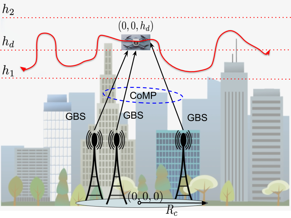
(a) Illustration of cooperative transmission

(b) Snapshot of a cluster-centric UAV-UE topology

Figure 1: Illustration of the proposed system model where BSs cooperatively serve high-altitude UAV-UEs via CoMP transmission. UAV-UEs can be either hovering at a fixed altitude $h_{d}$ or flying within minimum and maximum altitudes $h_{1}$ and $h_{2}$, respectively. In (b), the clusters are defined by a hexagonal grid, wherein BSs (orange diamonds) are distributed according to a homogeneous PPP and the UAV-UEs (black stars) are hovering above the centers of disjoint clusters.

II System Model

We consider a terrestrial cellular network in which BSs are distributed according to a two-dimensions (2D) homogeneous Poisson point process (PPP) $\Phi_{b}=\{b_{i}\in\mathbb{R}^{2},\forall i\in\mathbb{N}^{+}\}$ with intensity $\lambda_{b}$. All BSs have the same transmit power $P_{t}$, and are deployed at the same height $h_{\rm BS}$. We consider a number of high altitude cellular-connected UAV-UEs that can be either static or mobile based on the application. Particularly, the UAV-UEs are either hovering or moving at altitudes higher than the BS heights. We consider a cluster-centric UAV-UE model in which BSs are grouped into disjoint clusters modeled using a hexagonal grid with an inter-cluster center distance equal to $2R_{h}$, see Fig. 1. The area of each cluster is hence given by $A=2\sqrt{3}R_{h}^{2}$. For analytical convenience, we approximate the cluster area to a circle with the same area, i.e., with collaboration distance $R_{c}$ where $\pi R_{c}^{2}=2\sqrt{3}R_{h}^{2}$, and $R_{c}=\sqrt{\frac{2\sqrt{3}}{\pi}}R_{h}$. BSs belonging to the same cluster can cooperate to serve one UAV-UE within their cluster to mitigate the effect of LoS interference and, hence, enhance the UAV-UE cellular connectivity.

II-A Channel Model

We consider a wireless channel that is characterized by both large-scale and small-scale fading. For the large-scale fading, the channel between BS $i$ and an arbitrary UAV-UE is described by the LoS and non-line-of-sight (NLoS) components, which are considered separately along with their probabilities of occurrence [28]. This assumption is apropos for such ground-to-air (GTA) channels that often exhibit LoS communication (e.g., see [13] and [29]).

For small-scale fading, we adopt a Nakagami-$m_{v}$ model as done in [13] for the channel gain, whose probability distribution function (PDF) is given by: $f(\omega)=\frac{2m_{v}^{m_{v}}\omega^{2m_{v}-1}}{\Gamma(m_{v})}e^{-m_{v}\omega^{2}}$, where $m_{v}$, $v\in\{l,n\}$, is the fading parameter which is assumed to be an integer for analytical tractability, with $m_{l}>m_{n}$. In the special case when $m_{n}=1$, Rayleigh fading is recovered with an exponentially distributed instantaneous power, which can be used for the performance evaluation of ground users. Given that $\omega\sim$ Nakagami$(m_{v})$, it directly follows that the channel gain power $\chi=\omega^{2}\sim\Gamma(m_{v},1/m_{v})$, where $\Gamma(K,\theta)$ is a Gamma random variable (RV) with $K$ and $\theta$ denoting the shape and scale parameters, respectively. Hence, the PDF of channel power gain distribution will be: $f(\chi)=\frac{m_{v}^{m_{v}}\chi^{m-1}}{\Gamma(m_{v})}{\rm exp}\big{(}-m_{v}\chi\big{)}$.

3D blockage is characterized by the fraction $a$ of the total land area occupied by buildings, the mean number of buildings $\eta$ per $\text{\,}\mathrm{k}\mathrm{m}$², and the height of buildings modeled by a Rayleigh PDF with a scale parameter $c$. Hence, the probability of having a LoS communication from a BS at horizontal-distance $r_{i}$ from an arbitrary UAV-UE is given, similar to [25] and [29], as:

$$\mathbb{P}_{l}(r_{i})=\prod_{n=0}^{m}\Bigg{[}1-{\rm exp}\Big{(}-\frac{\big{(}h_{\rm BS}+\frac{h(n+0.5)}{m+1}\big{)}^{2}}{2c^{2}}\Big{)}\Bigg{]},$$ (1)

where $h$ represents the difference between the UAV-UE altitude and BS height, which depends on whether the UAV-UE is static or mobile, and $m=\lfloor\frac{r_{i}\sqrt{a\eta}}{1000}-1\rfloor$. Different terrain structures and environments can be considered by varying the tuple $(a,\eta,c)$. As previously discussed, the performance of relatively high-altitude UAV-UEs is limited by the LoS interference they encounter and reduced serving antenna gain (from the antennas’ side-lobes). We hence propose a multi-BS cooperative transmission scheme that mitigates inter-cell interference and, thus, improves the performance of high-altitude UAV-UEs. Hence, the antenna gain plus path loss for each component, i.e., LoS and NLoS, will be

$$\zeta_{v}(r_{i}) =A_{v}G_{s}d_{i}^{-\alpha_{v}}=A_{v}G_{s}\big{(}r_{i}^{2}+h^{2}\big{)}^{-\alpha_{v}/2},$$ (2)

where $d_{i}$ is the communication link distance, $v\in\{l,n\}$, $\alpha_{l}$ and $\alpha_{n}$ are the path loss exponents for the LoS and NLoS links, respectively, with $\alpha_{l}<\alpha_{n}$, and $A_{l}$ and $A_{n}$ are the path loss constants at the reference distance $d_{i}=$1\text{\,}\mathrm{m}$$ for the LoS and NLoS, respectively. $G_{s}$ is the antenna directivity gain of side-lobes between BS $i$ and an arbitrary UAV-UE since, at such high altitudes, UAV-UEs are served by the side-lobes of BS antennas [11]. The BS vertical antenna pattern is directional and typically down-tilted to account for GUEs. Given this setup, it is reasonable to assume that UAV-UEs are always served from the antennas’ side-lobes while the GUEs are served from the antennas’ main-lobes with antenna gains $G_{s}$ and $G_{m}$, respectively, where $G_{s}\ll G_{m}$.

Having defined our system model, next, we will consider two scenarios: Static UAV-UEs and mobile UAV-UEs. For each scenario, we will characterize the coverage probability of high altitude UAV-UEs that are collaboratively served from BSs within their cluster. The performance of collaboratively-served UAV-UEs is then compared to their terrestrial counterparts and to UAV-UEs under the nearest association scheme. Moreover, we will characterize the handover rate for mobile UAV-UEs and quantify the negative impact of mobility on their achievable performance.

III Coverage Probability of Static UAV-UEs

Hovering drones can provide appealing solutions for a wide range of applications such as traffic control and surveillance [30]. We here assume static UAV-UEs that hover at a fixed altitude $h_{d}$, where $h_{d}>h_{\rm BS}$. Hence, we set $h=h_{d}-h_{\rm BS}$ in (1) and (2). We also assume that BSs within one cluster cooperatively serve one UAV-UE whose projection on the ground is at the cluster center. Note that assuming such a cluster-center UAV-UE is mainly done for tractability, but its performance can be seen as an UB on the performance of a randomly located UAV-UE inside the cluster [31]. Given that a PPP is translation invariant with respect to the origin, for simplicity, we conduct the coverage analysis for a UAV-UE located at the origin in $\operatorname*{\mathbb{R}}^{2}$, referred to as the typical UAV-UE [32]. Next, we first characterize the serving distance distribution, and then, we employ it to derive upper and lower bounds on the coverage probability of static UAV-UEs.

III-A Serving Distance Distributions

Under the condition of having $\kappa$ serving BSs in the cluster of interest, the distribution of in-cluster BSs will follow a binomial point process (BPP) [32]. This BPP consists of $\kappa$ uniformly and independently distributed BSs in the cluster. The set of cooperative BSs is defined as $\Phi_{c}=\{b_{i}\in\Phi_{b}\cap\mathcal{B}(0,R_{c})\}$, where $\mathcal{B}(0,R_{c})$ denotes the ball centered at the origin $(0,0)\in\operatorname*{\mathbb{R}}^{2}$ with radius $R_{c}$. Recall that the typical UAV-UE is located at the origin in $\mathbb{R}^{2}$, i.e., $(0,0,h_{d})\in\mathbb{R}^{3}$. The 2D distances from the cooperative BSs to the typical UAV-UE are represented by $\boldsymbol{R}_{\kappa}=[R_{1},\dots,R_{\kappa}]$. Then, conditioning on $\boldsymbol{R}_{\kappa}=\boldsymbol{r}_{\kappa}$, where $\boldsymbol{r}_{\kappa}=[r_{1},\dots,r_{\kappa}]$, the conditional joint PDF of the serving distances is $f_{\boldsymbol{R}_{\kappa}}(\boldsymbol{r}_{\kappa})$. The $\kappa$ cooperative BSs can be seen as the $\kappa$-closest BSs to the cluster center from the PPP $\Phi_{b}$. Since the $\kappa$ BSs are independently and uniformly distributed in the cluster approximated by $\mathcal{B}(0,R_{c})$, the PDF of the horizontal distance from the origin to BS $i$ will be: $f_{R_{i}}(r_{i})=\frac{2r_{i}}{R_{c}^{2}}$, $0\leq r_{i}\leq R_{c}$, for any $i\in\mathcal{K}_{f}=\{1,\dots,\kappa\}$, where $\mathcal{K}_{f}$ is the set of collaborative BSs within the ball $\mathcal{B}(0,R_{c})$. From the independently and identically distributed (i.i.d.) property of BPP, the conditional joint PDF of the serving distances $\boldsymbol{R}_{\kappa}=[R_{1},\dots,R_{\kappa}]$ is expressed as $f_{\boldsymbol{R}_{\kappa}}(\boldsymbol{r}_{\kappa})=\prod_{i=0}^{\kappa}\frac{2r_{i}}{R_{c}^{2}}$.

III-B Performance of UAV-UEs

Under the condition of having $\kappa$ serving BSs, the received signal at the UAV-UE will be:

$$P =\underbrace{\sum_{i=1}^{\kappa}P_{v}(r_{i})\omega_{i}w_{i}Y_{0}}_{\text{desired signal}}+\underbrace{\sum_{k\in\Phi_{b}\setminus\mathcal{B}(0,R_{c})}P_{v}(u_{k})\omega_{k}w_{k}Y_{k}}_{\text{interference}}+\quad Z,$$ (3)

where the first term represents the desired signal from $\kappa$ collaborative BSs with $P_{v}^{2}(r_{i})=P_{t}\zeta_{v}(r_{i})$, $v\in\{l,n\}$, $\omega_{i}$ being the Nakagami-$m_{v}$ fading variable of the channel from BS $i$ to the UAV-UE, $w_{i}$ is the precoder used by BS $i$, and $Y_{0}$ is the channel input symbol that is sent by the cooperating BSs. The second term represents the inter-cluster interference, whose power is denoted as $I_{\rm out}$, where $Y_{j}$ is the transmitted symbol from interfering BS $j$ and $u_{j}$ is the horizontal distance between interfering BS $j$ and the UAV-UE; $Z$ is a circular-symmetric zero-mean complex Gaussian RV that models the background thermal noise.

As discussed earlier, UAV-UEs exhibit a LoS component which becomes dominant at relatively high altitudes. The LoS probability in (1) represents a delta function that goes from one to zero as $r_{i}$ increases. This implies that the probability of LoS communication from close BSs is higher than that of remote BSs. Hence, we consider that the desired signal is dominated by its LoS component where $v=l$, $m_{v}=m_{l}$, and $P_{v}(r_{i})=\sqrt{P_{t}}\zeta_{l}(r_{i})^{0.5}$. However, for the interfering signal, both LoS and NLoS components exist and, thus, we have: $P_{v}(u_{j})=\sqrt{P_{t}}\zeta_{v}(u_{j})^{0.5}$, $v\in\{l,n\}$. This is due to the fact that, as the LoS probability decreases with the interfering distance $u_{j}$, the LoS assumption becomes less practical for far but interfering BSs.

We assume that the channel state information (CSI) is available at the serving BSs. Hence, MRT can be adopted by BSs to maximize the received power at the typical UAV-UE. For the MRT, we have the precoder $w_{i}$ set as $w_{i}=\frac{\omega_{i}^{*}}{|\omega_{i}|}$, where $\omega_{i}^{*}$ is the complex conjugate of $\omega_{i}$. Assuming that $Y_{0}$ and $Y_{k}$ in (3) are independent zero-mean RVs of unit variance, and neglecting the thermal noise, the conditional $\mathrm{SIR}$ at the typical UAV-UE will then be:

$$\Upsilon_{|\boldsymbol{r}_{\kappa}} =\frac{P_{t}\Big{|}\sum_{i=1}^{\kappa}\zeta_{l}^{1/2}(r_{i})w_{i}\omega_{i}\Big{|}^{2}}{\sum_{k\in\Phi_{b}\setminus\mathcal{B}(0,R_{c})}\big{|}P_{v}(u_{k})\omega_{k}w_{k}\big{|}^{2}},$$ (4)

where $\Upsilon_{|\boldsymbol{r}_{\kappa}}$ is conditioned on the number of collaborative BSs $\kappa$, and on $\boldsymbol{R}_{\kappa}=\boldsymbol{r}_{\kappa}$. In (4), we have $\Big{|}\sum_{i=1}^{\kappa}\zeta_{l}^{1/2}(r_{i})w_{i}\omega_{i}\Big{|}^{2}$ representing the square of a weighted sum of $\kappa$ Nakagami-$m_{l}$ RVs. Since there is no known closed-form expression for a weighted sum of Nakagami-$m_{l}$ RVs, we use the Cauchy-Schwarz’s inequality to get an UB on a square of weighted sum as follows:

$$\Bigg{|}\sum_{i=1}^{\kappa}\zeta_{l}^{1/2}(r_{i})w_{i}\omega_{i}\Bigg{|}^{2}=\Bigg{|}\sum_{i=1}^{\kappa}\zeta_{l}^{1/2}(r_{i})\frac{\omega_{i}^{*}\omega_{i}}{|\omega_{i}|}\Bigg{|}^{2} =\Bigg{(}\sum_{i=1}^{\kappa}Q_{i}\Bigg{)}^{2}\leq\kappa\Bigg{(}\sum_{i=1}^{\kappa}Q_{i}^{2}\Bigg{)},$$ (5)

where $Q_{i}=\zeta_{l}^{1/2}(r_{i})\frac{\omega_{i}^{*}\omega_{i}}{|\omega_{i}|}=\zeta_{l}^{1/2}(r_{i})\omega_{i}$ is a scaled Nakagami-$m_{l}$ RV, and $i\in\mathcal{K}_{f}$. Since $\omega_{i}\sim$ Nakagami$(m_{l})$, from the scaling property of the Gamma PDF, $Q_{i}^{2}\sim\Gamma\big{(}K_{i}=m_{l},\theta_{i}=\zeta_{l}(r_{i})/m_{l}\big{)}$. To get a tractable statistical equivalence of a sum of $\kappa$ Gamma RVs with different scale parameters $\theta_{i}$, we adopt the method of sum of Gammas second-order moment match proposed in [33, Proposition 8]. It is shown that the equivalent Gamma distribution, denoted as $J\sim\Gamma(K,\theta)$, with the same first and second-order moments has the following parameters:

$$K=\frac{\Big{(}\sum_{i}{K_{i}\theta_{i}}\Big{)}^{2}}{\sum_{i}{K_{i}\theta_{i}^{2}}}=\frac{m_{l}\Big{(}\sum_{i}{\zeta_{l}(r_{i})}\Big{)}^{2}}{\sum_{i}{\Big{(}\zeta_{l}(r_{i})\Big{)}^{2}}}\quad\quad\text{and}\quad\quad\theta=\frac{\sum_{i}{K_{i}\theta_{i}^{2}}}{\sum_{i}K_{i}\theta_{i}}=\frac{\sum_{i}{\zeta_{l}(r_{i})^{2}}}{m_{l}\sum_{i}\zeta_{l}(r_{i})}.$$ (6)

The accuracy of the Gamma approximation can be easily verified via numerical simulations that are omitted due to space limitations. For tractability, we further upper bound the shape parameter $K$ using the Cauchy-Schwarz’s inequality as: $K\leq\frac{m_{l}\kappa\sum_{i}\big{(}\zeta_{l}(r_{i})\big{)}^{2}}{\sum_{i}\big{(}\zeta_{l}(r_{i})\big{)}^{2}}=m_{l}\kappa$, where, by definition, $m_{l}\kappa$ is integer. We shall also see shortly the tightness of this UB.

Next, we derive UB and LB expressions on the UAV-UE coverage probability. Our developed approach is novel in the sense that it adopts the Cauchy-Schwarz’s inequality and moment match of Gamma RVs to characterize an UB on the coverage probability, which is difficult to obtain exactly. The UAV-UE coverage probability conditioned on $\boldsymbol{R}_{\kappa}=\boldsymbol{r}_{\kappa}$ is given by

$$\mathbb{P}_{{\rm c}|\boldsymbol{r}_{\kappa}} \overset{(a)}{\leq}\mathbb{P}\Big{(}\frac{\kappa P_{t}\big{(}\sum_{i=1}^{\kappa}Q_{i}\big{)}^{2}}{I_{\rm out}}>\vartheta\Big{)}\overset{(b)}{\approx}\mathbb{P}\Big{(}\frac{\kappa P_{t}J}{I_{\rm out}}>\vartheta\Big{)},$$ (7)

where (a) follows from the Cauchy-Schwarz’s inequality, (b) follows from the Gamma approximation and rounding the shape parameter $K=m_{l}\kappa$, and $\vartheta$ is the $\mathrm{SIR}$ threshold. The coverage probability can be obtained as a function of the system parameters, particularly, the Nakagami fading parameter and collaboration distance, as stated formally in the following theorem.

Theorem 1.

An UB on the coverage probability of UAV-UEs cooperatively served from BSs within a collaboration distance $R_{c}$ can be derived as follows:

$$\mathbb{P}_{{\rm c}}=\sum_{\kappa=1}^{\infty}\mathbb{P}(n=\kappa)\int_{\boldsymbol{r_{\kappa}}=\boldsymbol{R_{c}}}^{\boldsymbol{\infty}}\mathbb{P}_{{\rm c}|\boldsymbol{r}_{\kappa}}^{l}\prod_{i=0}^{\kappa}\frac{2r_{i}}{R_{c}^{2}}\differential{\boldsymbol{r}_{\kappa}},$$ (8)

where the conditional coverage probability $\mathbb{P}_{{\rm c}|\boldsymbol{r}}^{l}=\lVert e^{\boldsymbol{T}_{K}}\rVert_{1}$, $\lVert.\rVert_{1}$ represents the induced $\ell_{1}$ norm, and $\boldsymbol{T}_{K}$ is the lower triangular Toeplitz matrix:

$$\boldsymbol{T}_{K}=\begin{bmatrix}t_{0}\\ t_{1}&t_{0}\\ \vdots&\vdots&\ddots\\ t_{K-1}&\dots&t_{1}&t_{0}\end{bmatrix};$$

$K=m_{l}\kappa$, $t_{i}=\frac{(-\varpi)^{i}}{(i)!}\Omega^{(i)}(\varpi)$, $\Omega^{(i)}(\varpi)=\frac{d^{i}}{d\varpi^{i}}\Omega(\varpi)_{|\boldsymbol{r}_{\kappa}}$, $\Omega(\varpi)_{|\boldsymbol{r}_{\kappa}}=-2\pi\lambda_{b}\int_{\nu=R_{c}}^{\infty}\Big{(}1-\delta_{l}\mathbb{P}_{l}(\nu)-\delta_{n}\mathbb{P}_{n}(\nu)\Big{)}\nu\differential{\nu}$, $\delta_{l}=\Big{(}1+\frac{\varpi P_{l}(\nu)^{2}}{m_{l}}\Big{)}^{-m_{l}}$, $\delta_{n}=\Big{(}1+\frac{\varpi P_{n}(\nu)^{2}}{m_{n}}\Big{)}^{-m_{n}}$, and $\varpi=\vartheta/\kappa P_{t}\theta$.

Proof.

Please see Appendix A. ∎

The main steps towards tractable coverage are summarized as follows [34]: We first derive the conditional log-Laplace transform $\Omega(\varpi)_{|\boldsymbol{r}_{\kappa}}$ of the aggregate interference. Then, we calculate the $i$-th derivative of $\Omega(\varpi)_{|\boldsymbol{r}_{\kappa}}$ to populate the entries $t_{i}$ of the lower triangular Toeplitz matrix $\boldsymbol{T}_{K}$. The conditional coverage probability can be then computed from $\mathbb{P}_{{\rm c}|\boldsymbol{r}}^{l}=\lVert e^{\boldsymbol{T}_{k}}\rVert_{1}$.

Important insights on the coverage probability can be obtained from (8). First, if the collaboration distance $R_{c}$ increases, both the probability $\mathbb{P}(n=\kappa)$ and the integrand value in (8) increase, and, thus, the coverage probability grows accordingly. Furthermore, the effect of the BS density $\lambda_{b}$ on the coverage probability is two-fold. On the one hand, the average number of BSs increases with $\lambda_{b}$ as characterized by $\mathbb{P}(n=\kappa)$, which results in a higher desired signal power. On the other hand, this advantage is counter-balanced by the increase in (LoS) interference power when $\lambda_{b}$ increases, as captured in the decaying exponential functions in (36). Additionally, this compact representation, i.e., $\mathbb{P}_{{\rm c}|\boldsymbol{r}}^{l}=\lVert e^{\boldsymbol{T}_{K}}\rVert_{1}$, leads to valuable system insights. For instance, the impact of the shape parameter $K=\kappa m_{l}$ on the intended channel gain $\Gamma(K,\theta)$ is rigorously captured by the finite sum representation in (34) of Appendix A, which is typically related to the collaboration distance $R_{c}$ and the Nakagami fading parameter $m_{l}$.

Next, we derive an LB on the coverage probability, which will lead to closed-form expressions for $t_{k}$, i.e., the entries populating $\boldsymbol{T}_{K}$ in (8). Given the high-altitude assumption of UAV-UEs, we will consider a special case when interfering BSs have dominant LoS communications to the typical UAV-UE, i.e, $\mathbb{P}_{l}(\nu)=1$ and $\mathbb{P}_{n}(\nu)=0$ in (8). Since this case results in higher interference power, this yields the derived coverage probability LB.

Corollary 1.

An LB on the coverage probability of the UAV-UEs can be computed from (8), where $\mathbb{P}_{{\rm c}|\boldsymbol{r}}^{l}=\lVert e^{\boldsymbol{T}_{K}}\rVert_{1}$, and the entries of $\boldsymbol{T}_{K}$ are given in closed-form expressions as

$$t_{k} \overset{}{=}\pi\lambda_{b}R_{ch}^{2}\Big{(}\textbf{1}\{k=0\}-c_{k}{}_{2}F_{1}(k+m_{l},k-\delta_{l};k+1-\delta_{l};-\varpi LR_{ch}^{-\alpha_{l}/2}m_{l})\Big{)},$$ (9)

where $c_{k}=\frac{\delta_{l}a_{k}\Gamma(k+m_{l})m_{l}^{-k}}{(\delta_{l}-k)\Gamma(k+1)\Gamma(m_{l})}$, $a_{k}=(\varpi LR_{ch}^{-\alpha_{l}/2})^{k}$, $\delta_{l}=\frac{2}{\alpha_{l}}$, $R_{ch}^{2}=R_{c}^{2}+h^{2}$, $\textbf{1}\{.\}$ is the indicator function, and ${}_{2}F_{1}(\cdot,\cdot;\cdot;\cdot)$ is the ordinary hypergeometric function.

Proof.

Please see Appendix B. ∎

For comparison purposes, next, we derive the UAV-UE coverage probability under the nearest association scheme.

Corollary 2.

The coverage probability of the UAV-UEs under the nearest association scheme is:

$$\mathbb{P}_{{\rm c}}=\int_{0}^{\infty}\mathbb{P}_{{\rm c}|r_{0}}^{l}f_{R_{0}}(r_{0})\differential{r_{0}},$$ (10)

where $\mathbb{P}_{{\rm c}|r_{0}}^{l}=\lVert e^{\boldsymbol{T}_{m_{l}}}\rVert_{1}$, $\boldsymbol{T}_{m_{l}}$ is defined as $\boldsymbol{T}_{K}$ in (8), with $\Omega(\varpi)=-2\pi\lambda_{b}\int_{\nu=r_{0}}^{\infty}\Big{(}1-\delta_{l}\mathbb{P}_{l}(\nu)-\delta_{n}\mathbb{P}_{n}(\nu)\Big{)}\nu\differential{\nu}$, $\varpi=\frac{\vartheta m_{l}}{P_{t}\zeta_{l}(r_{0})}$, and $f_{R_{0}}(r_{0})=2\pi\lambda_{b}r_{0}e^{-\pi\lambda_{b}r_{0}^{2}}$ is the 2D serving distance PDF.

Proof.

The proof follows directly from [13] and Theorem 1, and hence is omitted for brevity. ∎

(a) Inter-cluster half distance $R_{h}=$190\text{\,}\mathrm{m}$$

(b) SIR threshold $\vartheta=$0\text{\,}\mathrm{d}\mathrm{B}$$

Figure 2: The derived upper and lower bounds on the coverage probability of UAV-UEs are plotted versus the SIR threshold $\vartheta$ and collaboration distance $R_{c}$: $\lambda_{b}=$20\text{\,}\mathrm{k}\mathrm{m}^{-2}$$, $R_{\rm sim}=$20\text{\,}\mathrm{k}\mathrm{m}^{2}$$, $\alpha_{l}=2.09$, $\alpha_{n}=3.75$, $h_{\rm BS}=$30\text{\,}\mathrm{m}$$, $m_{l}=3$, $A_{L}=0.0088$, $A_{N}=0.0226$, $h_{d}=$120\text{\,}\mathrm{m}$$, $a=0.3$, $b=$300\text{\,}\mathrm{k}\mathrm{m}^{-2}$$, and $c=$20\text{\,}\mathrm{m}$$.

To verify the accuracy of our proposed approach, in Fig. 2, we show the theoretical UB and LB on the coverage probability of the UAV-UEs, and simulation of the UB based on (5). Fig. 2(a) shows that the Cauchy’s inequality-based UB is remarkably tight. Moreover, although the obtained UB expression in (8) is less tight, it still represents a reasonably tractable bound on the exact coverage probability. Hence, (8) can be treated as a proxy of the exact result. Recall that (5) is based on an UB on a square of a sum of Nakagami-$m_{l}$ RVs while the expression in (8) goes further by two more steps. First, we approximate the sum of Gamma RVs to an equivalent Gamma RV. Then, we round the shape parameter of the yielded Gamma RV to an integer $m_{l}\kappa$. Finally, the LB based on (9) can be also seen as a relatively looser bound than the UBs. As evident from Fig. 2, allowing CoMP transmission significantly enhances the coverage probability, e.g., from $28\%$ for the baseline scenario with nearest serving BSs to $60\%$ at $\vartheta=$ $-5\text{\,}\mathrm{d}\mathrm{B}$ (for an average of 2.5 cooperating BSs). In Fig. 2, the performance of UAV-UEs is also compared to that of their ground counterparts experiencing Rayleigh fading and NLoS communications. We assume that the BSs’ antennas are ideally down-tilted accounting for the GUEs, i.e., the antenna gains for desired and interfering signals are $G_{m}$ and $G_{s}$, respectively. Under such a setup, we observe that the coverage probability of GUEs substantially outperforms that of UAV-UEs, especially at high SIR thresholds. Fig. 2(b) shows the prominent effect of the collaboration distance $R_{c}$ on the coverage probability of ground and aerial UEs. We can see that for both kind of UEs, the coverage probability monotonically increases with $R_{c}$ since more BSs cooperate to serve the UEs when $R_{c}$ increases. Moreover, due to the down-tilt of the BSs’ antennas and LoS-dominated interference for UAV-UEs, the coverage probability of GUEs outperforms that of the UAV-UEs. However, we can see that the rate of coverage probability improvement with $R_{c}$, i.e., the slope, is higher for the UAV-UE. This can be interpreted by the fact that increasing $R_{c}$ yields more LoS signals within the desired signal side and subtracts them from the interference. Conversely, for GUEs, the transmission is dominated by NLoS signals and Rayleigh fading.

Having characterized the performance of static UAV-UEs, next, we turn our attention to applications in which the UAV-UEs can be mobile. It is anticipated that mobile UAV-UEs will span a wide variety of applications, e.g., flying taxis and delivery drones. Hence, it is quite important to ensure reliable connections in the presence of UAV-UE mobility by potentially mitigating the LoS interference through CoMP transmissions. Moreover, unlike the GUEs that can only move horizontally, UAV-UEs can fly in 3D space. Hence, a 3D mobility model is essential to convey a realistic description of the performance of mobile UAV-UEs. As a first step in this direction, we develop a novel 3D random waypoint (RWP) mobility model that effectively captures the vertical displacement of UAV-UEs, along with their typical 2D spatial mobility. The use of RWP mobility is motivated by its simplicity and tractability that is widely adopted in the mobility analysis in cellular networks [35, 36, 37, 38]. Moreover, as we will discuss shortly, it has tunable parameters that can be set to appropriately describe the mobility of different mobile nodes, ranging from walking or driving users to 3D UAVs, [23] and [38].

IV 3D Mobility and Handover Analysis

Next, a novel 3D RWP model is presented to describe the motions of UAV-UEs. We first illustrate the various elements of our proposed model. Then, we characterize the handover rate and handover probability for mobile UAV-UEs. Since we introduce the first study on 3D mobile UAV-UEs, for completeness, we consider two cases: UAV-UEs under CoMP transmissions, and UAV-UEs served by the nearest GBS.

In the classical 2D mobility model, the spatial motion is considered only through a displacement and an angle. However, for the UAV-UE, due to the mission requirements, and environmental and atmospherical conditions, the UAV-UEs must change their altitude and make vertical motions. For instance, due to variations in the altitudes of buildings, UAV-UEs might have frequent up and down displacements along their trajectories. Indeed, the vertical motion is always associated with the take-off and landing of UAV-UEs. This inherently triggers the concept of 3D mobility in 3D space.

First, recall that in a classical RWP mobility model [35, 36, 37, 38], the movement trace of a node (e.g., the UAV-UE) can be formally described by an infinite sequence of tuples: $\{(\boldsymbol{X}_{n-1},\boldsymbol{X}_{n},V_{n})\}$, $\forall\boldsymbol{X}_{n}\in\operatorname*{\mathbb{R}}^{3}$, and $n\in\mathbb{N}$, where $n$ is the movement epoch and $\boldsymbol{X}_{n}=(\varrho_{n},\phi_{n},z_{n})$ is the 3D cylindrical displacement of the UAV-UE at epoch $n$, see Fig. 3. During the $n$-th movement epoch, $\boldsymbol{X}_{n-1}$ denotes the starting waypoint, $\boldsymbol{X}_{n}$ denotes the target waypoint, and $V_{n}$ is the velocity. For simplicity, we assume that the UAV-UE moves with a constant velocity $\bar{\nu}$. However, further extensions to generalized PDFs of the velocity directly follow by the same methodology of analysis. Given the current waypoint $\boldsymbol{X}_{n-1}$, the next waypoint $\boldsymbol{X}_{n}$ is chosen such that the included angle $\phi_{n}$ between the projection of the vector $\boldsymbol{X}_{n-1}-\boldsymbol{X}_{n}$ on the $x$-$y$ plane and the abscissa is uniformly distributed on $[0,2\pi]$. We define the transition length as the Euclidean distance between two 3D successive waypoints, i.e., $u_{n}=\lVert\boldsymbol{X}_{n}-\boldsymbol{X}_{n-1}\rVert=\sqrt{\varrho_{n}^{2}+(z_{n}-z_{n-1})^{2}}$. Furthermore, the vertical displacement between two consecutive points, i.e., the change in $z$-axis, is also distributed according to a RV. We also let $\varphi_{n}$ be the acute angle of $U_{n}=\lVert\boldsymbol{X}_{n}-\boldsymbol{X}_{n-1}\rVert$ relative to the horizontal line $\rho_{n}$.

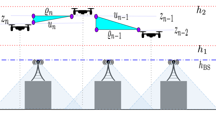
(a) A sample trace of the proposed 3D RWP mobility model

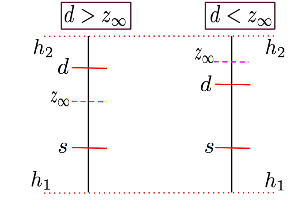
(b) Illustration of 1D RWP vertical mobility [23]

Figure 3: The proposed 3D mobility model for UAV-UEs which incorporates the typical 2D spatial RWP and 1D RWP for the vertical displacements.

For simplicity, the selection of waypoints is assumed to be independent and identical for each movement epoch [36]. Particularly, similar to [38], the horizontal transition lengths $\{\rho_{1},\rho_{2},\dots\}$ are chosen to be i.i.d. with the cumulative distribution function (CDF) $F_{\rho_{n}}(\varrho_{n})=1-{\rm exp}(-\pi\mu\varrho_{n}^{2})$, i.e., the spatial transition lengths are Rayleigh distributed in $\operatorname*{\mathbb{R}}^{2}$ with mobility parameter $\mu$. The corresponding displacement PDF is hence $f_{\rho_{n}}(\varrho_{n})=\frac{\partial F_{\rho_{n}}(\varrho_{n})}{\partial\varrho_{n}}=2\pi\mu\varrho_{n}e^{-\pi\mu\varrho_{n}^{2}}$. As also done in [23] and [22], we adopt a uniform distribution for the vertical displacement, however, the analysis for generalized PDFs can readily follow. In particular, we assume that $Z_{n}$ is uniformly distributed on $[h_{1},h_{2}]$, i.e., $Z_{n}\sim\operatorname*{\mathcal{U}}(h_{1},h_{2})$ and $f_{Z_{n}}(z_{n})=\frac{1}{h_{2}-h_{1}},\forall h_{1}\leq z_{n}\leq h_{2}$. We henceforth refer to $\hbar=h_{2}-h_{1}$ as altitude difference. Since the major restrictions of all drones’ operations are their flying altitudes, it is reasonable to assume that $Z_{n}$ is bounded by $h_{1}$ and $h_{2}$. For instance, UAVs cannot fly higher than certain altitudes (above ground level (AGL)) that are typically chosen below the cruising altitude of manned aircrafts. The UAVs also have an inherent minimum altitude of zero AGL. However, due to mission requirements as well as environmental and atmospherical conditions, it is reasonable to assume $h_{1}>0$. We further assume that $h_{1}>h_{\rm BS}$ for a high altitude UAV-UEs scenario. Finally, for the 3D displacement, we have $u_{n}=\sqrt{\varrho_{n}^{2}+(z_{n}-z_{n-1})^{2}}$. Since $U_{n}$, $\rho_{n}$, or $Z_{n}$ are i.i.d. RVs among different time epochs, we henceforth omit the epoch index.

Given the independence assumption between $Z$ and $\rho$, we obtain their joint PDF from $f_{\rho,Z}(\varrho,z)=f_{\rho}(\varrho)f_{Z}(z)=\frac{2\pi\mu\varrho}{\hbar}e^{-\pi\mu\varrho^{2}}$, $\forall h_{1}\leq z\leq h_{2},0\leq\varrho\leq\infty$. Under the proposed mobility model, different mobility patterns can be captured by choosing different mobility parameters $\mu$. For example, larger values of $\mu$ statistically implies that $\rho$ and, consequently, the 3D transition lengths $U$ are shorter. This means that the movement direction switch rates are higher. These values of the mobility parameter appropriately describe the motion of UAV-UEs frequently travelling between nearby hovering locations such as for the use case of aerial surveillance cameras. In contrast, smaller $\mu$ statistically implies that $\rho$ and, consequently, $U$ are longer and the corresponding movement direction switch rates are lower. These values of $\mu$ would be suitable to describe the motion of UAV-UEs traveling large distances such as for the use case of flying taxis and delivery drones. Given the PDFs of spatial and vertical motions, the PDF of the 3D displacement $f_{U}(u)$ is readily obtained in the next lemma.

Lemma 1.

The PDF of the 3D transition lengths $U$ is given by $f_{U}(u)=2\pi\mu ue^{-\pi\mu u^{2}}\Omega(\mu,\hbar)$, where $\Omega(\mu,\hbar)=\frac{\pi\hbar\sqrt{\mu}{\rm erfi}\left(\sqrt{\pi\mu}\hbar\right)-e^{\pi\mu\hbar^{2}}+1}{\pi\mu\hbar^{2}}$, and ${\rm erfi}(.)=\frac{-2i}{\sqrt{\pi}}\int_{0}^{x}e^{-t^{2}}dt$.

Proof.

We can reach this result by transforming the RVs $Z_{n}$, $Z_{n-1}$, and $\rho_{n}$ to $U_{n}$, where $u_{n}=\sqrt{\varrho_{n}^{2}+(z_{n}-z_{n-1})^{2}}$, with the details omitted due to space limitations. ∎

Remark 1.

If $h_{1}=h_{2}$, it can be easily verified that ${\rm lim}_{\hbar\to 0}\Omega(\mu,\hbar)\to 1$, and $f_{U}(u)=2\pi\mu ue^{-\pi\mu u^{2}}$. This shows that if the UAV-UE moves only along a horizontal plane, the PDF of the 3D displacement distance is reduced to its 2D counterpart, which verifies the correctness of the obtained 3D displacement distribution $f_{U}(u)$.

Having described the various elements of our proposed 3D RWP model, our immediate objective is to characterize the handover rate and handover probability for mobile UAV-UEs under CoMP transmissions and nearest association.

IV-A Handover Rate and Handover Probability for Nearest Association

Assume that a mobile UAV-UE is located at $\boldsymbol{X}_{n-1}$ and let $\boldsymbol{X}_{n-1}$ and $\boldsymbol{X}_{n}$ be two arbitrary successive waypoints. The handover rate is defined as the expected number of handovers per unit time. Hence, inspired from [38], we can compute the handover rate as follows. We first condition on an arbitrary position of the mobile UAV-UE $\boldsymbol{X}_{n}=\boldsymbol{x}_{n}$, and a given realization of the Poisson-Voronoi tessellation $\Phi_{b}$. Subsequently, the number of handovers will be equal to the number of intersections of the UAV-UE trajectory and the boundary of the Poisson-Voronoi tessellation. Then, by averaging over the spatial distribution of $\boldsymbol{X}_{n}$ and the distribution of Poisson-Voronoi tessellation, we derive the expected number of handovers. Alternatively, we notice that the number of handovers is equivalent to the number of intersections of the Poisson-Voronoi tessellation and the horizontal projection of the segment $\big{[}\boldsymbol{X}_{n-1},\boldsymbol{X}_{n}\big{]}$ on the $x$-$y$ plane. Therefore, following [38, 39, 40], the expected number of handovers during one movement epoch will be: $\mathbb{E}\big{[}N\big{]}=\frac{2}{\pi}\sqrt{\frac{\lambda_{b}}{\mu}}$. The handover rate is then the ratio of the expected number of handovers during one movement $\mathbb{E}\big{[}N\big{]}$ to the mean time of one transition movement $\mathbb{E}\big{[}T\big{]}$. Since we have $\mathbb{E}[T]=\mathbb{E}[\frac{U}{V}]=\frac{\mathbb{E}[U]}{\bar{\nu}}=\frac{\Omega(\mu,\hbar)}{2\sqrt{\mu}\bar{\nu}}$, where $\mathbb{E}[U]=\frac{\Omega(\mu,\hbar)}{2\sqrt{\mu}}$, then, the handover rate will be:

$$H=\frac{\mathbb{E}[N]}{\mathbb{E}[T]}=\frac{2}{\pi}\sqrt{\frac{\lambda_{b}}{\mu}}\Bigg{/}\frac{\Omega(\mu,\hbar)}{2\sqrt{\mu}\bar{\nu}}=\frac{4\bar{\nu}\sqrt{\lambda_{b}}}{\pi\Omega(\mu,\hbar)}.$$ (11)

Remark 2.

Unlike the handover rate for 2D RWP [38, 39, 40], $H$ in (11) is a function of the mobility parameter $\mu$ through $\Omega(\mu,\hbar)$. This captures the fact that, in the case of an UAV-UE, since each stochastically generated horizontal displacement is accompanied with a vertical one, the handover rate depends on $\mu$ that affects the vertical displacement switch rates.

Next, to characterize the coverage probability of mobile UAV-UEs, we use the concept of handover probability. Similar to [40] and [41], given the current location of a mobile UAV-UE, the handover probability is defined as the probability that there exists a BS closer than the serving BS after a unit time. From Fig. 4(a), for two arbitrary consecutive waypoints $\boldsymbol{X}_{n-1}=(\varrho_{n-1},\phi_{n-1},z_{n-1})$ and $\boldsymbol{X}_{n}=(\varrho_{n},\phi_{n},z_{n})$, the horizontal speed of the UAV-UE from waypoint $\boldsymbol{X}_{n-1}$ to waypoint $\boldsymbol{X}_{n}$ is $\nu_{h}=\bar{\nu}{\rm cos}(\varphi_{n})$, where $\varphi_{n}={\rm arccos}\Big{(}\frac{\varrho_{n}}{\sqrt{\varrho_{n}^{2}+(z_{n}-z_{n-1})^{2}}}\Big{)}$. It is also assumed that the angle $\phi_{n}$ is taken with respect to the direction of connection as shown in Fig. 4(a). Define $\boldsymbol{q}_{n-1}$ and $\boldsymbol{q}_{n}$ in $\operatorname*{\mathbb{R}}^{2}$ as the horizontal projections of $\boldsymbol{X}_{n-1}$ and the location reached by the UAV-UE after a unit time, respectively. Fig. 4(a) illustrates that the UAV-UE is first associated with its nearest BS located at $\boldsymbol{q}_{0}$, i.e., there are no BSs in the ball of radius $r_{0}=\lVert\boldsymbol{q}_{n-1}-\boldsymbol{q}_{0}\rVert$ centered at $\boldsymbol{q}_{n-1}$. Using the law of cosines, $\boldsymbol{q}_{n}$ is at distance $R=\sqrt{r_{0}^{2}+(\bar{\nu}{\rm cos}(\varphi_{n}))^{2}+2r_{0}(\bar{\nu}{\rm cos}(\varphi_{n}))cos(\phi_{n})}$ from the BS located at $\boldsymbol{q}_{0}$.

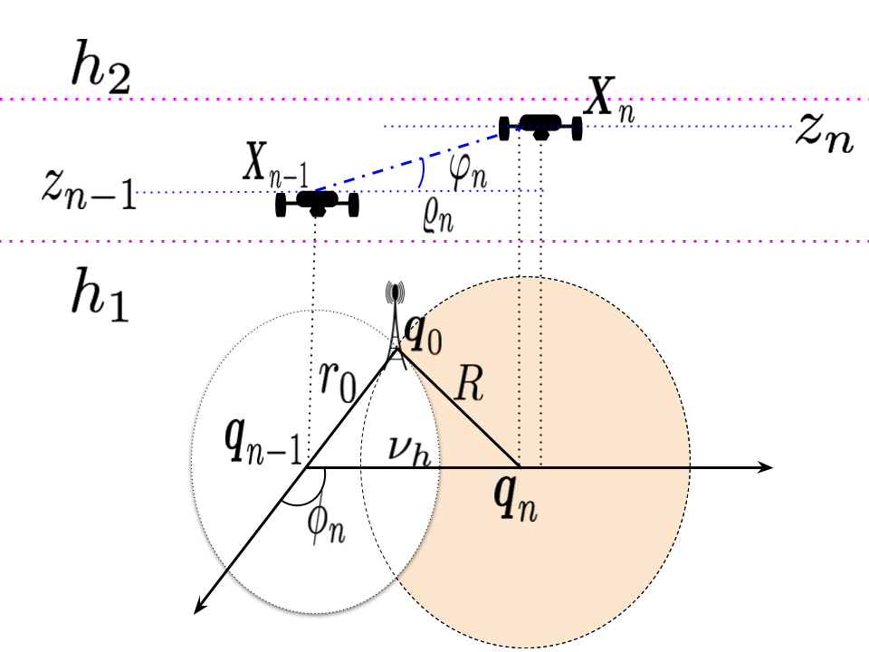
(a) Nearest association handover scenario

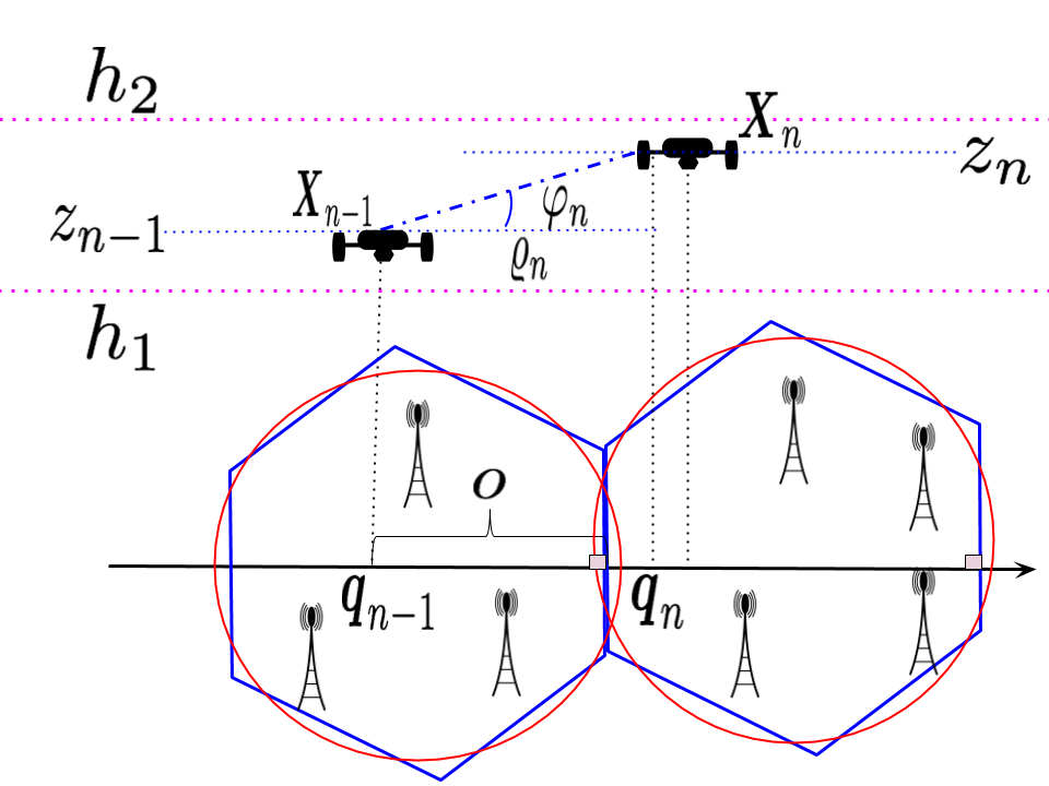
(b) Inter-CoMP handover scenario

Figure 4: The probability of handover is computed based on the network geometry.

The handover occurs only if another BS becomes closer to $\boldsymbol{q}_{n}$ than the serving BS located at $\boldsymbol{q}_{0}$, i.e., when there is at least one BS in the shaded area in Fig. 4(a). Therefore, given $\{r_{0},z_{n-1},z_{n},\varrho_{n},\phi_{n}\}$, the conditional probability of handover is $\mathbb{P}(H|r_{0},z_{n-1},z_{n},\varrho_{n},\phi_{n})$

$$=\mathbb{P}\Big{(}\mathcal{B}(\boldsymbol{q}_{n},R)\setminus\mathcal{B}(\boldsymbol{q}_{n-1},r_{0})>0|r_{0},z_{n-1},z_{n},\varrho_{n},\phi_{n}\Big{)}\overset{(a)}{=}1-e^{-\lambda_{b}\big{|}\mathcal{B}(\boldsymbol{q}_{n},R)\setminus\mathcal{B}(\boldsymbol{q}_{n-1},r_{0})\big{|}}$$

$$=1-e^{-\pi\lambda_{b}(R^{2}-r_{0}^{2})}\overset{}{=}1-e^{-\pi\lambda_{b}\big{(}r_{0}^{2}+(\bar{\nu}{\rm cos}(\varphi_{n}))^{2}+2r_{0}\bar{\nu}{\rm cos}(\varphi_{n})cos(\phi_{n})-r_{0}^{2}\big{)}},$$ (12)

where (a) follows from the void probability of PPP. $\mathcal{B}(\boldsymbol{q}_{n},R)$ represents the ball with radius $R$ centered at $\boldsymbol{q}_{n}$ and $\mathcal{B}(\boldsymbol{q}_{n-1},r_{0})$ is excluded from $\mathcal{B}(\boldsymbol{q}_{n},R)$ since the BS located at $\boldsymbol{q}_{0}$ is the nearest BS to $\boldsymbol{q}_{n-1}$. Finally, averaging over $Z_{n-1},Z_{n},\rho_{n}$, and $\phi_{n}$, where $\phi_{n}\sim\operatorname*{\mathcal{U}}(0,2\pi)$, we get

$$\mathbb{P}(H|r_{0}) =1-\mathbb{E}_{\rho_{n},Z_{n},Z_{n-1},\phi_{n}}\Big{[}e^{-\pi\lambda_{b}\big{(}(\bar{\nu}{\rm cos}(\varphi_{n}))^{2}+2r_{0}(\bar{\nu}{\rm cos}(\varphi_{n}))cos(\phi_{n})\big{)}}\Big{]}.$$ (13)

For the special case in which the UAV-UE moves radially away from the serving BS, i.e., $\phi_{n}=0$, next, we obtain a tractable yet accurate UB on the handover probability. This assumption is reasonable, particularly, if the UAV-UE follows a horizontally-direct path subject only to vertical fluctuations due to mission, environmental, and atmospheric conditions.

Lemma 2.

An UB on the conditional probability of handover is given by

$$\mathbb{P}(H|r_{0}) \overset{}{=}1-e^{-\frac{2\lambda_{b}r_{0}\bar{\nu}}{\sqrt{\pi}\mu\hbar^{2}}\psi(\mu,\hbar)}e^{-\pi\lambda_{b}\zeta(\mu,\hbar)},$$ (14)

where $\psi(\mu,\hbar)=\pi\hbar^{2}\mu G_{2,3}^{2,2}\Big{(}\hbar^{2}\pi\mu\Big{|}\begin{array}[]{c}\frac{1}{2},\frac{1}{2}\\ 0,1,-\frac{1}{2}\\ \end{array}\Big{)}-G_{2,3}^{2,2}\Big{(}\hbar^{2}\pi\mu\Big{|}\begin{array}[]{c}1,\frac{3}{2}\\ 1,2,0\\ \end{array}\Big{)}$, $G_{p,q}^{m,n}$ denotes the Meijer $G$ function, defined as

$$G_{p,q}^{m,n}=\Big{(}x\Big{|}\begin{array}[]{c}a_{1},\dots,a_{p}\\ b_{1},\dots,b_{q}\\ \end{array}\Big{)}=\frac{1}{2\pi i}\int\frac{\prod_{j=1}^{m}\Gamma(b_{j}+s)\prod_{j=1}^{n}\Gamma(1-a_{j}+s)}{\prod_{j=n+1}^{p}\Gamma(a_{j}+s)\prod_{j=m+1}^{q}\Gamma(1-b_{j}+s)}x^{s}\differential{s},$$ (17)

and $\zeta(\mu,\hbar)=\bar{\nu}^{2}\Big{(}1-\frac{2\pi\mu}{\hbar^{2}}\int_{0}^{\hbar}(\hbar-p)p^{2}e^{\pi\mu p^{2}}\Gamma\left(0,\pi p^{2}\mu\right)\differential{p}$ ).

Proof.

Please see Appendix C. ∎

From (14), it is intuitive to see that $\mathbb{P}(H|r_{0})$ increases with $\bar{\nu}$ and $\lambda_{b}$ because there will be a higher probability of handover when the UAV-UE velocity is higher, and the network is denser. Moreover, $\mathbb{P}(H|r_{0})$ decreases as the term $\mu\hbar^{2}$ increases. This reveals important insights on the effect of the altitude difference $\hbar$ and the density $\mu$. Particularly, the handover probability decreases when the UAV-UE jointly has higher direction switch rates (higher $\mu$) and larger altitude difference $\hbar$. Next, we obtain the handover rate for UAV-UEs under CoMP transmissions.

IV-B Inter-CoMP Handover Rate and Handover Probability

We define the number of handovers $\mathbb{E}[N]$ as the number of intersections of the horizontal projection of the segment $\big{[}\boldsymbol{X}_{n-1},\boldsymbol{X}_{n}\big{]}$ and the boundaries of disjoint clusters whose inter-cluster center distance is $2R_{h}$, as discussed in Section II. The hexagonal cell has six sides of length $l=\frac{2R_{h}}{\sqrt{3}}$. Following the Buffon’s needle approach for hexagonal cells [40], we next obtain the inter-CoMP handover rate.

Proposition 1.

The inter-CoMP handover rate for a network of disjoint clusters whose inter-cluster center distance is $2R_{h}$ is given by

$$H=\frac{\mathbb{E}[N]}{\mathbb{E}[T]}=2\frac{\pi\hbar^{2}\mu G_{2,3}^{2,2}\Big{(}\hbar^{2}\pi\mu\big{|}\begin{array}[]{c}\frac{1}{2},\frac{1}{2}\\ 0,1,-\frac{1}{2}\\ \end{array}\Big{)}-G_{2,3}^{2,2}\Big{(}\hbar^{2}\pi\mu\big{|}\begin{array}[]{c}1,\frac{3}{2}\\ 1,2,0\\ \end{array}\Big{)}}{\pi\sqrt{\pi}R_{h}\hbar^{2}\mu}\bar{\nu}.$$ (22)

Proof.

Please see Appendix D. ∎

(a) Nearest association scenario

(b) CoMP transmission scenario

Figure 5: The probability of handover is plotted versus network parameters for nearest association and CoMP transmission schemes ($\bar{\nu}=$30\text{\,}\mathrm{k}\mathrm{m}\mathrm{h}$$, $\mu=$300\text{\,}\mathrm{k}\mathrm{m}^{-2}$$, $h_{1}=$100\text{\,}\mathrm{m}$$).

We now characterize the UAV-UE inter-CoMP handover probability. To keep the analysis simple, we consider a special case in which the UAV-UE moves perpendicularly to the inter-cluster boundaries, as shown in Fig. 4(b). As discussed in Section IV-A, this is a practical assumption for a UAV-UE that follows a horizontally straight path subject only to vertical fluctuations. Moreover, since these boundaries represent virtual borders between disjoint clusters, the assumption that such boundaries are in a direction perpendicular to the UAV-UE trajectory is quite reasonable. Hence, the UAV-UE moves by a horizontal distance $\bar{\nu}{\rm cos}(\varphi_{n})$ in a unit of time in a direction perpendicular to the inter-cluster boundaries. A handover occurs if this travelled horizontal distance is larger than the distance $o$ to the cluster side, formally stated as

$$\mathbb{P}(H|o) =\mathbb{P}\big{(}\frac{\bar{\nu}\varrho_{n}}{\sqrt{\varrho_{n}^{2}+(z_{n}-z_{n-1})^{2}}}>o\big{)}=\mathbb{P}\big{(}\varrho_{n}>\frac{o(z_{n}-z_{n-1})}{\sqrt{\bar{\nu}^{2}-o^{2}}}\big{)}$$

$$=\mathbb{E}_{Z_{n},Z_{n-1}}\int_{\varrho_{n}=\frac{o(z_{n}-z_{n-1})}{\sqrt{\bar{\nu}^{2}-o^{2}}}}^{\infty}2\pi\mu\varrho_{n}e^{-\pi\mu\varrho_{n}^{2}}\differential{\varrho_{n}}$$ (23)

$$\overset{(a)}{=}\mathbb{E}_{Z_{n},Z_{n-1}}e^{-\pi\mu\big{(}\frac{o^{2}(z_{n}-z_{n-1})^{2}}{\bar{\nu}^{2}-o^{2}}\big{)}}\overset{(b)}{=}\mathbb{E}_{p}e^{-\pi\mu p^{2}\frac{o^{2}}{\bar{\nu}^{2}-o^{2}}}$$

$$\overset{(c)}{=}\frac{1}{\hbar^{2}}\frac{\hbar\sqrt{\frac{\mu o^{2}}{\bar{\nu}^{2}-o^{2}}}{\rm erf}\left(\sqrt{\pi}\hbar\sqrt{\frac{o^{2}}{\bar{\nu}^{2}-o^{2}}}\sqrt{\mu}\right)+\frac{e^{-\pi\mu\hbar^{2}\frac{o^{2}}{\bar{\nu}^{2}-o^{2}}}-1}{\pi}}{\frac{\mu o^{2}}{\bar{\nu}^{2}-o^{2}}}$$ (24)

$$=\frac{1}{\hbar}\frac{{\rm erf}\left(\sqrt{\pi}\hbar\sqrt{\frac{\mu o^{2}}{\bar{\nu}^{2}-o^{2}}}\right)}{\sqrt{\frac{\mu o^{2}}{\bar{\nu}^{2}-o^{2}}}}+\frac{1}{\pi\hbar^{2}}\frac{e^{-\pi\mu\hbar^{2}\frac{o^{2}}{\bar{\nu}^{2}-o^{2}}}-1}{\frac{\mu o^{2}}{\bar{\nu}^{2}-o^{2}}},$$ (25)

where (a) follows from solving the integral of (23), (b) follows from change of variables $p=z_{n}-z_{n-1}$, with $f_{P}(p)=\frac{\hbar-|p|}{\hbar^{2}},-\hbar\leq p\leq\hbar$, and (c) follows from taking the expectation with respect to (w.r.t.) $p$. Recall that $O$ is a RV that models the distance between the UAV-UE and the inter-cluster boundaries. Averaging over $O$ given that $f_{O}(o)=\frac{1}{2R_{h}},0<o<2R_{h}$, we get $\mathbb{P}(H)$. However, we observe that if $o>\bar{\nu}$, the handover probability will be zero since the UAV-UE can not travel the distance $o$ in a unit of time, hence, we have

$$\mathbb{P}(H) \overset{}{=}\frac{1}{2R_{h}\hbar}\int_{o=0}^{\bar{\nu}}\frac{{\rm erf}\left(\sqrt{\pi}\hbar\sqrt{\frac{\mu o^{2}}{\bar{\nu}^{2}-o^{2}}}\right)}{\sqrt{\frac{\mu o^{2}}{\bar{\nu}^{2}-o^{2}}}}+\frac{1}{2\pi R_{h}\hbar^{2}}\int_{o=0}^{\bar{\nu}}\frac{e^{-\pi\mu\hbar^{2}\frac{o^{2}}{\bar{\nu}^{2}-o^{2}}}-1}{\frac{\mu o^{2}}{\bar{\nu}^{2}-o^{2}}}.$$ (26)

Fig. 5 verifies the accuracy of the obtained handover probabilities. Fig. 5(a) presents the handover probability versus BSs’ intensity $\lambda_{b}$ under the nearest association scheme. The figure shows that the obtained UB in (14) is quite tight. It is also noted that as long as the UAV-UE has frequent vertical movements, i.e., larger $\hbar$, the handover probability is lower since the effective horizontal travelled distance becomes shorter. The handover probability also monotonically increases with $\lambda_{b}$ since a higher rate of handover occurs for denser networks. Fig. 5(b) shows the inter-CoMP handover probability versus the inter-cluster center distance $2R_{h}$. The handover probability monotonically decreases with $R_{h}$ since a lower rate of handover is anticipated when the cluster size increases. Next, we will use our proposed RWP model to obtain the coverage probability of 3D mobile UAV-UEs under the nearest association and CoMP transmission schemes.

V Coverage Probability of Mobile UAV-UEs

Next, we will use the obtained handover probabilities in (14) and (26) to quantify the coverage probability of mobile UAV-UEs under the nearest association and CoMP transmissions, respectively. It is worth highlighting that (8) represents the probability that a static UAV-UE is in coverage with neither mobility nor handover considered. However, mobile UAV-UEs are susceptible to frequent handovers that would negatively impact their performance. For instance, handover typically results in dropped connections and causes longer service delays. In fact, higher handover rates lead to a higher risk of quality-of-service (QoS) degradation.

To account for the user mobility, similar to [40, 41, 42], we consider a linear function that reflects the cost of handovers. Under this model, the UAV-UE coverage probability can be defined as:

$$P_{c}(\bar{\nu},\mu,\beta)=\mathbb{P}(\Upsilon\geq\vartheta,\bar{H})+(1-\beta)\mathbb{P}(\Upsilon\geq\vartheta,H),$$ (27)

where the first term represents the probability that the UAV-UE is in coverage and no handover occurring. Besides, the second term is the probability that the UAV-UE is in coverage and handover occurs penalized by a handover cost, where $\beta\in[0,1]$ represents the probability of connection failure due to handover. The coefficient $\beta$, in effect, measures the system sensitivity to handovers, which highly depends on the hysteresis margin and ping-pong rate [39, 40, 41, 42]. Our goal is to obtain the coverage probability of a mobile UAV-UE for a given handover penalty $\beta$ [40]. After some manipulations, we can rewrite (27) as

$$P_{c}(\bar{\nu},\mu,\beta)=(1-\beta)\mathbb{P}(\Upsilon\geq\vartheta|r_{0})+\beta\mathbb{P}(\Upsilon\geq\vartheta,\bar{H}|r_{0}).$$ (28)

To obtain $P_{c}(\bar{\nu},\mu,\beta)$, we first need to calculate the statistical distribution of the UAV-UE altitude for our proposed 3D mobility model. As shown in Fig. 3(b), the 3D mobility model defines the vertical movement of the UAV-UE in a finite region $[h_{1},h_{2}]$, referred to as vertical 1D RWP as in [23]. Initially, at time instant $t_{0}$, the UAV-UE is at an arbitrary altitude $h_{0}$ selected uniformly from the interval $[h_{1},h_{2}]$. Then, at next time epoch $t_{1}$, this UAV-UE at $h_{0}$ selects a new random waypoint $h_{1}$ uniformly in $[h_{1},h_{2}]$, and moves towards it (along with the spatial movement characterized by $f_{\rho_{n}}(\varrho_{n})$). Once the UAV-UE reaches $h_{1}$, it repeats the same procedure to find the next destination altitude and so on. After a long running time, the steady-state altitude distribution converges to a nonuniform distribution $F_{Z_{\infty}}(z_{\infty})$ [35], where $Z_{\infty}$ is a RV representing the steady state vertical location of the UAV-UE. Note that random waypoints refer to the altitude of a UAV-UE at each time epoch, which is uniformly-distributed in $[h_{1},h_{2}]$, while vertical transitions are the differences in the UAV-UE altitude throughout its trajectory. While the random waypoints are independent and uniformly-distributed by definition, the random lengths of vertical transitions are not statistically independent. This is because the endpoint of one movement epoch is the starting point of the next epoch. In [35], it is shown that $F_{Z_{\infty}}(z_{\infty})=\frac{\mathbb{E}[L_{z_{\infty}}]}{\mathbb{E}[L]}$, where $L_{z_{\infty}}$ and $L$ denote the length $\lVert z_{\infty}-h_{1}\rVert$, and the entire movement length at any given epoch, respectively. From [35], we have $\mathbb{E}[L]=\frac{\hbar}{3}$ and $\mathbb{E}[L_{z_{\infty}}]$ can be similarly derived from:

$$\mathbb{E}[L_{z_{\infty}}]=\int_{s=h_{1}}^{h_{2}}\int_{d=h_{1}}^{h_{2}}l_{z}(s,d)f_{S}(s)f_{D}(d)\differential{d}\differential{s},$$ (29)

where $s$ and $d$ refer to the source and destination of a movement, respectively; $f_{S}(s)=f_{D}(d)=\frac{1}{\hbar}$, $h_{1}\leq s,d\leq h_{2}$, see Fig. 3(b). Because of the symmetry of $s$ and $d$, it is sufficient to restrict the calculation to epochs with $s<d$, and then multiply the result by a factor of 2. A necessary condition for $l_{z_{\infty}}(s,d)\neq 0$ is that $s\leq z_{\infty}$. From Fig. 3(b), if $d\leq z_{\infty}$, we have $l_{z_{\infty}}(s,d)=d-s$, however, if $d>z_{\infty}$, we get $l_{z_{\infty}}(s,d)=z_{\infty}-s$, which yields

$$\mathbb{E}[L_{z_{\infty}}] =\frac{2}{\hbar^{2}}\int_{s=h_{1}}^{z_{\infty}}\int_{d=s}^{z_{\infty}}(d-s)\differential{d}\differential{s}+\frac{2}{\hbar^{2}}\int_{s=h_{1}}^{z_{\infty}}\int_{d=z_{\infty}}^{h_{2}}(z_{\infty}-s)\differential{d}\differential{s}$$

$$=\frac{2}{\hbar^{2}}\big{(}-\frac{h_{1}^{3}}{6}+\frac{h_{1}^{2}h_{2}}{2}-h_{1}h_{2}z_{\infty}+\frac{h_{1}z_{\infty}^{2}}{2}+\frac{h_{2}z_{\infty}^{2}}{2}-\frac{z_{\infty}^{3}}{3}\big{)}.$$ (30)

Therefore, the PDF of $Z_{\infty}$ is given by

$$f_{Z_{\infty}}(z_{\infty}) =\frac{\partial F_{Z_{\infty}}(z_{\infty})}{\partial z_{\infty}}=\frac{\partial}{\partial z_{\infty}}\frac{\mathbb{E}[L_{z_{\infty}}]}{\mathbb{E}[L]}=\frac{h_{1}z_{\infty}+h_{2}z_{\infty}-h_{1}h_{2}-z_{\infty}^{2}}{\hbar^{3}/6}\quad\forall h_{1}<z_{\infty}<h_{2},$$ (31)

and the corresponding mean is given by $L_{z_{\infty}}=\mathbb{E}[Z_{\infty}]=\frac{1}{2\hbar^{3}}\big{(}h_{2}^{4}-h_{1}^{4}+2h_{1}^{3}h_{2}-2h_{1}h_{2}^{3}\big{)}$. Next, we will use the derived PDF $f_{Z_{\infty}}(z_{\infty})$, along with the probability of handover from the previous section, to fully characterize $P_{c}(\bar{\nu},\mu,\beta)$ under the nearest association and CoMP transmissions.

V-A Coverage Probability for Nearest Association

Next, we derive the coverage probability of a mobile UAV-UE under the nearest association scheme. Observing (28), for a given $\beta$, we must compute $\mathbb{P}(\Upsilon\geq\vartheta,\bar{H}|r_{0})$ to obtain $P_{c}(\bar{\nu},\mu,\beta)$. The former probability is basically the joint event of being in coverage and no handover occurs. We adopt the tight UB on the handover probability obtained in (14), where $\mathbb{P}(\bar{H},r_{0})=1-\mathbb{P}(H,r_{0})$ is the conditional probability of no handover. Unlike static UAV-UEs, under the 3D RWP model, both the altitude of the UAV-UE and the horizontal distance $R_{0}$ to the nearest BS are RVs. Since $R_{0}$ and $Z_{\infty}$ are two independent RVs, we have $f_{R_{0},Z_{\infty}}(r_{0},z_{\infty})=f_{R_{0}}(r_{0})f_{Z_{\infty}}(z_{\infty})$.

We assume that the UAV-UE has an arbitrary long trajectory that passes through nearly all SIR states. Therefore, the average SIR through a randomly selected UAV-UE trajectory is inferred from a stationary PPP analysis. This assumption, which is adopted in [40, 42, 41] for GUEs, is practically reasonable for mobile UAV-UEs such as flying taxis and delivery drones that typically have sufficiently long trajectories. Given the handover probability in (14) and the linear function in (28), the UAV-UE coverage probability under the nearest association scheme is given below.

Theorem 2.

The coverage probability of a 3D mobile UAV-UE associated with its nearest BS is

$$P_{c}(\bar{\nu},\mu,\beta) =2(1-\beta)\pi\lambda_{b}\times\int_{h_{1}}^{h_{2}}\int_{0}^{\infty}r_{0}e^{-\pi\lambda_{b}r_{0}^{2}}\mathbb{P}_{{\rm c}|r_{0},z_{\infty}}^{l}f_{Z_{\infty}}(z_{\infty})\differential{r_{0}}\differential{z_{\infty}}+$$

$$2\beta\pi\lambda_{b}e^{-\pi\lambda_{b}\zeta(\mu,\hbar)}\times\int_{h_{1}}^{h_{2}}\int_{0}^{\infty}r_{0}e^{-\pi\lambda_{b}r_{0}^{2}}e^{-\frac{2\lambda_{b}r_{0}\bar{\nu}}{\sqrt{\pi}\mu\hbar^{2}}\psi(\mu,\hbar)}\mathbb{P}_{{\rm c}|r_{0},z_{\infty}}^{l}f_{Z_{\infty}}(z_{\infty})\differential{r_{0}}\differential{z_{\infty}},$$ (32)

where $\mathbb{P}_{{\rm c}|r_{0},z_{\infty}}^{l}=\lVert e^{\boldsymbol{T}_{m_{l}}}\rVert_{1}$, $\boldsymbol{T}_{m_{l}}$ is defined as $\boldsymbol{T}_{K}$ in (8), with $\Omega(\varpi)_{|r_{0},z_{\infty}}=-2\pi\lambda_{b}\int_{\nu=r_{0}}^{\infty}\big{(}1-\delta_{l}\mathbb{P}_{l}(\nu)-\delta_{n}\mathbb{P}_{n}(\nu)\big{)}\nu\differential{\nu}$, $\delta_{l}=\Big{(}1+\frac{\varpi P_{t}A_{l}G_{s}(\nu^{2}+z_{\infty}^{2})^{-\alpha_{l}/2}}{m_{l}}\Big{)}^{-m_{l}}$, $\delta_{n}=\Big{(}1+\frac{\varpi P_{t}A_{n}G_{s}(\nu^{2}+z_{\infty}^{2})^{-\alpha_{n}/2}}{m_{n}}\Big{)}^{-m_{n}}$, and $\varpi=\frac{\vartheta m_{l}}{P_{t}A_{l}G_{s}(r_{0}^{2}+z_{\infty}^{2})^{-\alpha_{l}/2}}$; $\psi(\mu,\hbar)$ and $\zeta(\mu,\hbar)$ are given in Lemma 2.

Proof.

The first term in (2) is obtained directly from (28) and Corollary 2, where the UAV-UE altitude $h_{d}$ is replaced with the RV $z_{\infty}$ whose PDF is given in (31). Additionally, the second term in (2) represents the joint event of no handover and being in coverage, which is computed based on $\mathbb{P}(H|r_{0},\phi)$ in (14). ∎

It is clear from (2) that, if $\beta=1$, the first term vanishes and the UAV-UE will be in coverage only if there is no handover associated with its mobility. This is because the handover will always cause connection failure. Moreover, since it is hard to directly obtain insights from (2) on the effect of the altitude $z_{\infty}$ and the altitude difference $\hbar$, several numerical results based on (2) will be shown in Section VI to provide key practical insights. Next, we similarly derive the coverage probability of a mobile UAV-UE under CoMP transmission.

V-B Coverage Probability for CoMP Transmission

Similar to Section V-A, we employ the handover probability in (26) and the linear function in (28) to obtain the coverage probability under CoMP transmission. The probability of inter-cluster handover $\mathbb{P}(H)$ is derived in (26) assuming that the UAV-UE moves perpendicular to the cluster boundaries. To compute $\mathbb{P}(\Upsilon\geq\vartheta,\bar{H})$ in (28), the joint PDF of the serving distances needs to be characterized given the random location of the UAV-UE along its trajectory. However, for tractability, we consider the joint serving distances when the UAV-UE horizontal projection is at the cluster center. Therefore, the obtained performance can be seen as an UB on the performance of a randomly located UAV-UE. This assumption is in line with prior work [31] and the analysis for static UAV-UEs, where we sought an UB on the coverage probability.

Since $\boldsymbol{R}_{\kappa}=[R_{1},\dots,R_{\kappa}]$ and $Z_{\infty}$ are independent RVs, their joint PDF is $f_{\boldsymbol{R}_{\kappa},Z_{\infty}}(\boldsymbol{r}_{\kappa},r_{0},z_{\infty})=f_{\boldsymbol{R}_{\kappa}}(\boldsymbol{r}_{\kappa})f_{Z_{\infty}}(z_{\infty})$. Given (26) and (28), an UB on the coverage probability of a mobile UAV-UE under CoMP transmissions is obtained in the next theorem.

Theorem 3.

An UB on the coverage probability of a 3D mobile UAV-UE cooperatively served via CoMP transmission from BSs within a collaboration distance $R_{c}$ is given by:

$$\mathbb{P}_{{\rm c}}=\big{(}1-\beta+\beta\times\mathbb{P}(\bar{H})\big{)}\sum_{\kappa=1}^{\infty}\mathbb{P}(n=\kappa)\int_{h_{1}}^{h_{2}}\int_{\boldsymbol{r_{\kappa}}=\boldsymbol{R_{c}}}^{\boldsymbol{\infty}}\mathbb{P}_{{\rm c}|\boldsymbol{r}_{\kappa},z_{\infty}}^{l}f_{Z_{\infty}}(z_{\infty})\prod_{i=0}^{\kappa}\frac{2r_{i}}{R_{c}^{2}}\differential{\boldsymbol{r}_{\kappa}}\differential{z_{\infty}},$$ (33)

where $\mathbb{P}(\bar{H})=1-\mathbb{P}(H)$ from (26), $\mathbb{P}_{{\rm c}|\boldsymbol{r}_{\kappa},z_{\infty}}^{l}=\lVert e^{\boldsymbol{T}_{K}}\rVert_{1}$, and $\boldsymbol{T}_{K}$ is as defined in (8), with $\Omega(\varpi)_{|\boldsymbol{r}_{\kappa},z_{\infty}}=-2\pi\lambda_{b}\int_{\nu=R_{c}}^{\infty}\Big{(}1-\delta_{l}\mathbb{P}_{l}(\nu)-\delta_{n}\mathbb{P}_{n}(\nu)\Big{)}\nu\differential{\nu}$, $\delta_{l}=\Big{(}1+\frac{\varpi P_{t}A_{l}G_{s}(\nu^{2}+z_{\infty}^{2})^{-\alpha_{l}/2}}{m_{l}}\Big{)}^{-m_{l}}$, $\delta_{n}=\Big{(}1+\frac{\varpi P_{t}A_{n}G_{s}(\nu^{2}+z_{\infty}^{2})^{-\alpha_{n}/2}}{m_{n}}\Big{)}^{-m_{n}}$, $\varpi=\frac{\vartheta}{\kappa P_{t}\theta}$, $\theta=\frac{\sum_{i}^{\kappa}{\zeta_{l}(r_{i})^{2}}}{m_{l}\sum_{i}^{\kappa}\zeta_{l}(r_{i})}$, and $\zeta_{l}(r_{i})=A_{l}G_{s}\big{(}r_{i}^{2}+z_{\infty}^{2}\big{)}^{-\alpha_{l}/2}$.

Proof.

The proof follows from (28) and Theorem 1, and is analogous to Theorem 2. ∎

The effect of $\beta$ on the coverage probability in (33) can be interpreted in a similar way to the nearest association scheme in (2). Moreover, conditioning on $Z_{\infty}=z_{\infty}$, and for a given $\beta$ in (33), the yielded expression holds the same insights as for static UAV-UEs in Section III-B. In particular, what the Nakagami fading parameter $m_{l}$, antenna down-tilting angle, and the collaboration distance $R_{c}$ entail for the performance of mobile UAV-UEs is similar to the that of static UAV-UEs. Finally, a simple lower bound on the mobile UAV-UE coverage probability can be obtained similar to Corollary 1, with the detailed omitted due to space limitation.

VI Simulation Results and Analysis

TABLE I: Simulation Parameters

Description	Parameter	Value	Description	Parameter	Value
LoS path-loss exponent	$\alpha_{l}$	2.09	$\mathrm{SIR}$ threshold	$\vartheta$	$0\text{\,}\mathrm{dB}$
NLoS path-loss exponent	$\alpha_{n}$	3.75	BSs’ intensity	$\lambda_{b}$	20 BSs/$\text{\,}\mathrm{k}\mathrm{m}$2
LoS path-loss constant	$A_{l}$	$-41.1\text{\,}\mathrm{d}\mathrm{B}$	Inter-cluster center distance	$2R_{h}$	$380\text{\,}\mathrm{m}$
NLoS path-loss constant	$A_{n}$	$-32.9\text{\,}\mathrm{d}\mathrm{B}$	Antenna main-lobe gain	$G_{m}$	$10\text{\,}\mathrm{d}\mathrm{B}$
Nakagami fading parameter (LoS)	$m_{l}$	3	Antenna side-lobe gain	$G_{s}$	$-3.01\text{\,}\mathrm{d}\mathrm{B}$
Nakagami fading factor (NLoS)	$m_{n}$	1	BS antenna height	$h_{\textrm{BS}}$	$30\text{\,}\mathrm{m}$
Area fraction occupied by buildings	$a$	0.3	UAV-UE altitude	$h_{d}$	$120\text{\,}\mathrm{m}$
Density of buildings	$\eta$	$300\text{\,}\mathrm{k}\mathrm{m}^{-2}$	Simulation area	$R_{\rm sim}$	$20\text{\,}\mathrm{k}\mathrm{m}^{2}$
Buildings height Rayleigh parameter	$c$	$20\text{\,}\mathrm{m}$	Mean altitude of mobile UAV-UEs	$L_{z_{\infty}}$	$150\text{\,}\mathrm{m}$

(a) UAV-UE coverage probability versus its altitude $h_{d}$

(b) UAV-UE coverage probability versus BS’s intensity $\lambda_{b}$

Figure 6: The derived upper and lower bounds on the static UAV-UE coverage probability are plotted versus the UAV-UE altitude $h_{d}$ and BSs’ intensity $\lambda_{b}$.

For our simulations, we consider a network having the parameter values indicated in Table I. In Fig. 6, we show the effect of the UAV-UE altitude and BSs’ intensity on the coverage probability of static UAV-UEs, with that of GUEs plotted for comparison. Fig. 6(a) shows that the coverage probability of UAV-UEs monotonically decreases as $h_{d}$ increases. This is because, as the UAV-UEs altitude increases, the signal power decreases while the LoS interference becomes dominant. Fig. 6(a) also shows that the derived UB on the coverage probability in (8) is considerably tight. Meanwhile, Fig. 6(b) illustrates the effect of BSs’ intensity $\lambda_{b}$ on the performance of UAV-UEs. Except for the nearest association scheme, the coverage probability improves with $\lambda_{b}$ since more BSs cooperate to serve the aerial (and ground) UEs. However, when the UAV-UE associates to its nearest BS, the effect of interference increases as the network becomes denser.

(a) $\bar{\nu}=$50\text{\,}\mathrm{k}\mathrm{m}\mathrm{h}$$, $\mu=$300\text{\,}\mathrm{k}\mathrm{m}^{-2}$$

(b) $\hbar=$30\text{\,}\mathrm{m}$$, $\mu=$300\text{\,}\mathrm{k}\mathrm{m}^{-2}$$

(c) $\beta=0.5$, $\mu=$100\text{\,}\mathrm{k}\mathrm{m}^{-2}$$, $\vartheta=$-10\text{\,}\mathrm{d}\mathrm{B}$$

Figure 7: Effect of the 3D mobility on the performance of aerial and UEs when they are associated with their nearest BSs. In (c), H-static refers to a UAV-UE that only moves in the vertical direction within an altitude difference $\hbar$.

Next, we study the impact of 3D mobility on the performance of UAV-UEs. We further compare the performance of UAV-UEs with their ground counterparts moving horizontally with the same velocity $\bar{\nu}$. In Fig. 7, the handover rate and coverage probability of mobile aerial and ground UEs associated with their nearest BSs are investigated. Fig. 7(a) plots the handover rate versus $\lambda_{b}$ at different values of the altitude difference $\hbar$. Fig. 7(a) shows that the analytical result in (11) matches the simulation result quite well. As is the case for typical Poisson-Voronoi models, the handover rate grows linearly with the square root of the BS’s intensity $\sqrt{\lambda_{b}}$. Moreover, the handover rate decreases as $\hbar$ increases, which implies that a UAV-UE having frequent up and down motions along its trajectory is susceptible to lower rates of handover. We also note that the handover rate of UAV-UEs is upper bounded by that of GUEs at $\hbar=0$. Fig. 7(b) shows the effect of the UAV-UE speed $\bar{\nu}$ on its handover rate. Intuitively, the handover rate increases as $\bar{\nu}$ increases since the UAV-UE stays shorter time in the area covered by each BS, i.e., shorter sojourn time. Finally, Fig. 7(c) investigates the effect of mobility on the UAV-UE coverage probability given an arbitrary handover penalty $\beta$. Notice that the coverage probability decreases as $\bar{\nu}$ increases since this leads to higher handover probability (penalized by $\beta$). Moreover, the altitude difference $\hbar$ has a marginal effect on the coverage probability of UAV-UEs. This is attributed to the fact that the increase of the altitude difference $\hbar$ for mobile UAV-UEs while keeping the same average flying altitude $L_{z_{\infty}}$ relatively yields the same average coverage probability.

In Fig. 8, we evaluate the effect of the 3D mobility on the UAV-UE performance under CoMP transmissions. Fig. 8(a) shows that the inter-CoMP handover rate monotonically decreases as $R_{c}$ increases since the UAV-UE would have a longer sojourn time in each cluster. Moreover, the handover rate is shown to decrease as $\hbar$ increases, i.e., when the UAV-UE has frequent up and down motions along its trajectory. We also note that the handover rate of UAV-UEs is upper bounded by that of GUEs, with $\hbar=0$. Fig. 8(b) shows the effect of the UAV-UE velocity $\bar{\nu}$ on the inter-CoMP handover. We note that this handover rate also increases as $\bar{\nu}$ increases since the UAV-UE will have a shorter sojourn time in each cluster. Finally, Fig. 8(c) shows the effects of the UAV-UE velocity and altitude difference on the UAV-UE coverage probability. Fig. 8(c) shows that the UB on the coverage probability, characterized in Theorem 3, slightly decreases as $\bar{\nu}$ increases, which corresponds to a higher handover rate (penalized by $\beta$). This slight decrease is essentially because as the inter-cluster distance becomes larger, the probability of handover decreases and its effect gradually vanishes. Similar to the nearest association scheme, the altitude difference $\hbar$ has a minor effect on the coverage probability of UAV-UEs. In addition to its impact on the coverage probability, the mobility of UAV-UEs can decrease their throughput, particularly, when accounting for the handover execution time [42].

(a) $\bar{\nu}=$30\text{\,}\mathrm{k}\mathrm{m}\mathrm{h}$$, $\mu=$300\text{\,}\mathrm{k}\mathrm{m}^{-2}$$

(b) $\mu=$100\text{\,}\mathrm{k}\mathrm{m}^{-2}$$, $\hbar=$50\text{\,}\mathrm{m}$$

(c) $\mu=$100\text{\,}\mathrm{k}\mathrm{m}^{-2}$$, $\beta=1$

Figure 8: Effect of the 3D mobility on the performance of aerial and ground UEs when they are served via CoMP transmission with the inter-cluster center distance set equal to $2R_{h}$. In (c), H-static refers to an UAV-UE that only moves in the vertical direction within an altitude difference $\hbar$.

VII Conclusion

In this paper, we have proposed a novel framework for cooperative transmission that can be leveraged to provide reliable connectivity and omnipresent mobility support for UAV-UEs. In order to analytically characterize the performance of UAV-UEs, we have employed Cauchy’s inequality and moment approximation of Gamma RVs to derive upper and lower bounds on the UAV-UE coverage probability. Moreover, we have developed a novel 3D RWP model that allowed us to explore the role of UAV-UEs’ mobility in cellular networks, particularly, to quantify the handover rate and the impact of their mobility on the achievable performance. For both static and mobile UAV-UEs, we have shown allowing CoMP transmission significantly improves the achievable coverage probability, e.g., from $28\%$ for the baseline scenario with nearest serving BSs, to $60\%$ for static UAV-UEs. Furthermore, comparing the performance of UAV-UEs to GUEs, it is shown that the coverage probability of a UAV-UE is always upper bounded by that of a GUE owing to the down-tilted antenna pattern and LoS-dominated interference for UAV-UEs. Our results for the case of mobile UAV-UEs have also revealed that their handover rate and handover probability decrease as the altitude difference increases, i.e., in the case of frequent up and down motions of the UAV-UEs along their trajectory. Moreover, while the altitude difference has a minor effect on the coverage probability of mobile UAV-UEs, their velocity noticeably degrades their coverage probability.

Appendix A Proof of Theorem 1

We proceed to obtain an UB on the coverage probability as follows:

$$\mathbb{P}\Big{(}\frac{\kappa P_{t}J}{I_{\rm out}}>\vartheta\Big{)}=\mathbb{P}\Big{(}\kappa P_{t}J>\vartheta I_{\rm out}\Big{)}=\mathbb{E}_{I_{\rm out}}\Bigg{[}\mathbb{P}\Big{(}\kappa P_{t}J>\vartheta I_{\rm out}\Big{)}\Bigg{]}$$

$$\overset{(a)}{\approx}\mathbb{E}_{I_{\rm out}}\Big{[}\sum_{i=0}^{K-1}\frac{(\vartheta/\kappa P_{t}\theta)^{i}}{i!}I_{\rm out}^{i}{\rm exp}\Big{(}-\frac{\vartheta}{\kappa P_{t}\theta}I_{\rm out}\Big{)}\Big{]}\overset{(b)}{=}\mathbb{E}_{I_{\rm out}}\Big{[}\sum_{i=0}^{K-1}\frac{(-\varpi)^{i}}{i!}\frac{d^{i}}{d\varpi^{i}}\mathcal{L}_{I_{\rm out}|\boldsymbol{r}_{\kappa}}(\varpi)\Big{]},$$ (34)

where (a) follows from the PDF of Gamma RV $J$ with parameters $\theta$ given in (6), and $K=m_{l}\kappa$; (b) follows from $\varpi=\frac{\vartheta}{\kappa P_{t}\theta}$, along with the Laplace transform of interference, i.e., the RV $I_{\rm out}$. Next, we derive the Laplace transform of interference:

$$\mathcal{L}_{I_{\rm out}|\boldsymbol{r}_{\kappa}}(\varpi) =\mathbb{E}_{I_{\rm out}}\Big{[}e^{-\varpi I_{\rm out}}\Big{]}=\mathbb{E}\Bigg{[}e^{-\varpi\sum_{j\in\Phi_{b}\setminus\mathcal{B}(0,R_{c})}\varpi\chi_{j}P(u_{j})^{2}}\Bigg{]}=\mathbb{E}_{\Phi_{b},\chi_{j}}\Bigg{[}\prod_{j\in\Phi_{b}\setminus\mathcal{B}(0,R_{c})}e^{-\varpi\chi_{j}P(u_{j})^{2}}\Bigg{]}$$

$$\overset{(a)}{=}{\rm exp}\Bigg{(}-2\pi\lambda_{b}\int_{\nu=R_{c}}^{\infty}\Big{(}1-\mathbb{E}_{\chi}e^{-\varpi\chi P(\nu)^{2}}\Big{)}\nu\differential{\nu}\Bigg{)}$$ (35)

$$\overset{(b)}{=}{\rm exp}\Bigg{(}-2\pi\lambda_{b}\int_{\nu=R_{c}}^{\infty}\Big{(}1-\delta_{l}\mathbb{P}_{l}(\nu)-\delta_{n}\mathbb{P}_{n}(\nu)\Big{)}\nu\differential{\nu}\Bigg{)}\overset{(c)}{=}e^{\Omega(\varpi)_{|\boldsymbol{r}_{\kappa}}},$$ (36)

where $\delta_{l}=\Big{(}1+\frac{\varpi P_{l}(\nu)^{2}}{m_{l}}\Big{)}^{-m_{l}}$, and $\delta_{n}=\Big{(}1+\frac{\varpi P_{n}(\nu)^{2}}{m_{n}}\Big{)}^{-m_{n}}$; (a) follows from the probability generating functional (PGFL) of PPP along with Cartesian to polar coordinates conversion [32], (b) follows from the moments of the Gamma RV $\chi\sim\Gamma(m_{v},1/m_{v})$ modeling the interfering channel gain, and (c) follows from $\Omega(\varpi)_{|\boldsymbol{r}_{\kappa}}=-2\pi\lambda_{b}\int_{\nu=R_{c}}^{\infty}\Big{(}1-\delta_{l}\mathbb{P}_{l}(\nu)-\delta_{n}\mathbb{P}_{n}(\nu)\Big{)}\nu\differential{\nu}$. In [34], it is proved that $\sum_{i=0}^{K-1}\frac{(-\varpi)^{i}}{i!}\mathcal{L}_{I|\boldsymbol{r}_{\kappa}}^{(i)}(\varpi)=\sum_{i=0}^{K-1}p_{i}$, where $p_{i}=\frac{(-\varpi)^{i}}{i!}\mathcal{L}_{I|\boldsymbol{r}_{\kappa}}^{(i)}(\varpi)$ can be computed from the recursive relation: $p_{i}=\sum_{l=0}^{i-1}\frac{i-l}{i}p_{l}t_{i-l}$, with $t_{i-1}=\frac{(-\varpi)^{i-1}}{(i-1)!}\Omega^{(i-1)}(\varpi)$, and $\Omega^{(i-1)}(\varpi)=\frac{d^{i-1}}{d\varpi^{i-1}}\Omega(\varpi)_{|\boldsymbol{r}_{\kappa}}$. After some algebraic manipulation as in [34], $\mathbb{P}_{{\rm c}|\boldsymbol{r}}^{l}$ can be expressed in a compact form $\mathbb{P}_{{\rm c}|\boldsymbol{r}}^{l}=\lVert e^{\boldsymbol{T}_{k}}\rVert_{1}$, where $\lVert.\rVert_{1}$ represents the induced $\ell_{1}$ norm, and $\boldsymbol{T}_{K}$ is the lower triangular Toeplitz matrix whose entries are $t_{i}$, $i=|\{1,\dots,K\}$. This completes the proof.

Appendix B Proof of Corollary 1

We first write the exponent power of (35) as

$$\Omega(\varpi)_{|\boldsymbol{r}_{\kappa}} =-2\pi\lambda_{b}\mathbb{E}_{\chi}\int_{\nu=R_{c}}^{\infty}\big{(}1-e^{-\varpi\chi P(\nu)^{2}}\big{)}\nu\differential{\nu}\overset{(a)}{=}-2\pi\lambda_{b}\mathbb{E}_{\chi}\int_{\nu=R_{c}}^{\infty}\big{(}1-e^{-\varpi L\chi(\nu^{2}+h^{2})^{-\alpha_{l}/2}}\big{)}\nu\differential{\nu},$$

where (a) follows from $P(\nu)^{2}=P_{t}A_{l}G_{s}\big{(}\nu^{2}+h^{2}\big{)}^{-\alpha_{l}/2}$ and substituting $L=P_{t}A_{l}G_{s}$. Let $z=\nu^{2}+h^{2}$, and $\differential{z}=2\nu\differential{\nu}$, we hence get

$$\Omega(\varpi)_{|\boldsymbol{r}_{\kappa}} =-\pi\lambda_{b}\mathbb{E}_{\chi}\int_{z=R_{c}^{2}+h^{2}}^{\infty}\big{(}1-e^{-\varpi L\chi z^{-\alpha_{l}/2}}\big{)}\differential{z}.$$ (37)

By changing the variables $y=z^{-\alpha_{l}/2}$, $z=y^{-2/\alpha_{l}}$, and $\differential{z}=\frac{-2}{\alpha_{l}}y^{\frac{-2}{\alpha_{l}}-1}\differential{y}$, and solving the reproduced integrals as in [43], we get

$$\Omega(\varpi)_{|\boldsymbol{r}_{\kappa}} \overset{}{=}\pi\lambda_{b}R_{ch}^{2}-\delta_{l}\pi\lambda_{b}(\varpi L)^{\delta_{l}}\mathbb{E}_{\chi}\Big{[}\chi^{\delta_{l}}\gamma(-\delta_{l},\varpi L\chi R_{ch}^{-\alpha_{l}/2})\Big{]}$$

$$\overset{(a)}{=}\pi\lambda_{b}R_{ch}^{2}-\delta_{l}\pi\lambda_{b}(\varpi L)^{\delta_{l}}\mathbb{E}_{\chi}\Big{[}\chi^{\delta_{l}}\epsilon{}_{1}F_{1}(-\delta_{l};1-\delta_{l};-\varpi L\chi R_{ch}^{-\alpha_{l}/2})\Big{]},$$ (38)

where $R_{ch}^{2}=R_{c}^{2}+h^{2}$, $\delta_{l}=\frac{2}{\alpha_{l}}$, $\epsilon=\frac{(\varpi L\chi)^{-\delta_{l}}R_{ch}^{2}}{\delta_{l}}$, and $\gamma(s,x)=\int_{0}^{x}t^{s-1}e^{-t}$ is the lower incomplete Gamma function; (a) follows from ${}_{1}F_{1}(s;s+1;-x)=\frac{s}{x^{s}}\gamma(s,x)$, where ${}_{1}F_{1}(\cdot;\cdot;\cdot)$ is the confluent hypergeometric function of the first kind. By rearranging (38), we can obtain

$$\Omega(\varpi)_{|\boldsymbol{r}_{\kappa}} =\pi\lambda_{b}R_{ch}^{2}\Bigg{(}1-\mathbb{E}_{\chi}\Big{[}{}_{1}F_{1}(-\delta_{l};1-\delta_{l};-\varpi L\chi R_{ch}^{-\alpha_{l}/2})\Big{]}\Bigg{)}.$$ (39)

The non-zero terms in $\boldsymbol{T}_{k}$ can be then determined from:

$$t_{k} =\frac{(-\varpi)^{k}}{k!}\Omega(\varpi)_{|\boldsymbol{r}_{\kappa}}^{(k)}=\pi\lambda_{b}R_{ch}^{2}\frac{(-\varpi)^{k}}{k!}\frac{d^{k}}{d\varpi^{k}}\Bigg{[}1-\mathbb{E}_{\chi}\Big{[}{}_{1}F_{1}(-\delta_{l};1-\delta_{l};-\varpi L\chi R_{ch}^{-\alpha_{l}/2})\Big{]}\Bigg{]}$$

$$=\pi\lambda_{b}R_{ch}^{2}\mathbb{E}_{\chi}\Bigg{[}\frac{(-\varpi)^{k}}{k!}(-L\chi R_{ch}^{-\alpha_{l}/2})^{k}\frac{d^{k}}{d(-\varpi L\chi R_{ch}^{-\alpha_{l}/2})^{k}}\Big{[}1-{}_{1}F_{1}(-\delta_{l};1-\delta_{l};-\varpi L\chi R_{ch}^{-\alpha_{l}/2})\Big{]}\Bigg{]}$$

$$=\pi\lambda_{b}R_{ch}^{2}\mathbb{E}_{\chi}\Bigg{[}\frac{(\varpi L\chi R_{ch}^{-\alpha_{l}/2})^{k}}{k!}\frac{d^{k}}{d(-\varpi L\chi R_{ch}^{-\alpha_{l}/2})^{k}}\Big{[}1-{}_{1}F_{1}(-\delta_{l};1-\delta_{l};-\varpi L\chi R_{ch}^{-\alpha_{l}/2})\Big{]}\Bigg{]}$$

$$\overset{(b)}{=}\pi\lambda_{b}R_{ch}^{2}\Bigg{(}\textbf{1}\{k=0\}-\frac{(\varpi LR_{ch}^{-\alpha_{l}/2})^{k}}{\Gamma(k+1)}\frac{\delta_{l}}{(\delta_{l}-k)}\mathbb{E}_{\chi}\Big{[}\chi^{k}{}_{1}F_{1}(k-\delta_{l};k+1-\delta_{l};-\varpi L\chi R_{ch}^{-\alpha_{l}/2})\Big{]}\Bigg{)},$$

where (b) follows from the derivatives for hypergeometric functions: $\frac{d^{k}}{dz^{k}}{}_{1}F_{1}(a;b;z)=\frac{\prod_{p=0}^{k-1}(a+p)}{\prod_{p=0}^{k-1}(b+p)}\times{}_{1}F_{1}(a+k;b+k;z)$. By letting $a_{k}=(\varpi LR_{ch}^{-\alpha_{l}/2})^{k}$, we get

$$t_{k} =\pi\lambda_{b}R_{ch}^{2}\Bigg{(}\textbf{1}\{k=0\}-\frac{\delta_{l}a_{k}}{(\delta_{l}-k)\Gamma(k+1)}\mathbb{E}_{\chi}\Big{[}\chi^{k}{}_{1}F_{1}(k-\delta_{l};k+1-\delta_{l};-\varpi L\chi R_{ch}^{-\alpha_{l}/2})\Big{]}\Bigg{)}.$$

Lastly, to get a closed-form expression for $t_{k}$, we average over $\chi\sim\Gamma(m_{l},1/m_{l})$ as follows:

$$t_{k} =\pi\lambda_{b}R_{ch}^{2}\Bigg{(}\textbf{1}\{k=0\}-b_{k}\int_{\chi=0}^{\infty}\chi^{k+m_{l}-1}e^{-m_{l}\chi}{}_{1}F_{1}(k-\delta_{l};k+1-\delta_{l};-\varpi LR_{ch}^{-\alpha_{l}/2}\chi)\differential{\chi}\Bigg{)}$$

$$=\pi\lambda_{b}R_{ch}^{2}\Bigg{(}\textbf{1}\{k=0\}-b_{k}\Gamma(k+m_{l})m_{l}^{-(k+m_{l})}{}_{2}F_{1}(k+m_{l},k-\delta_{l};k+1-\delta_{l};-\varpi LR_{ch}^{-\alpha_{l}/2}m_{l})\Bigg{)}$$

$$\overset{(c)}{=}\pi\lambda_{b}R_{ch}^{2}\Big{(}\textbf{1}\{k=0\}-c_{k}{}_{2}F_{1}(k+m_{l},k-\delta_{l};k+1-\delta_{l};-\varpi LR_{ch}^{-\alpha_{l}/2}m_{l})\Big{)},$$ (40)

where $b_{k}=\frac{\delta_{l}a_{k}m_{l}^{m_{l}}}{(\delta_{l}-k)\Gamma(k+1)\Gamma(m_{l})}$, $c_{k}=\frac{m_{l}^{m_{l}}}{\Gamma(m_{l})}b_{k}=\frac{\delta_{l}a_{k}\Gamma(k+m_{l})m_{l}^{-k}}{(\delta_{l}-k)\Gamma(k+1)\Gamma(m_{l})}$, and (c) follows from solving the integral in (B) [44, Eq. 7.525] and rearranging the right hand side. This completes the proof.

Appendix C Proof of Lemma 2

When $\varphi_{n}=0$, the conditional probability of handover can be expressed as

$$\mathbb{P}(H|r_{0}) =1-\mathbb{E}_{\rho_{n},Z_{n},Z_{n-1}}\Big{[}e^{-\pi\lambda_{b}\big{(}(\bar{\nu}{\rm cos}(\varphi_{n}))^{2}+2r_{0}\bar{\nu}{\rm cos}(\varphi_{n})\big{)}}\Big{]}$$ (41)

$$\overset{(a)}{\leq}1-\underbrace{e^{-\pi\lambda_{b}\mathbb{E}_{\rho_{n},Z_{n},Z_{n-1}}\big{(}\frac{2r_{0}\bar{\nu}\varrho_{n}}{\sqrt{\varrho_{n}^{2}+(z_{n}-z_{n-1})^{2}}}+(\frac{\bar{\nu}\varrho_{n}}{\sqrt{\varrho_{n}^{2}+(z_{n}-z_{n-1})^{2}}})^{2}\big{)}}}_{\mathbb{P}(\bar{H}|r_{0})},$$ (42)

where (a) follows from Jensen’s inequality, with $\mathbb{P}(\bar{H}|r_{0})$ being an LB on the probability of no handover conditioned on $r_{0}$. We obtain $\mathbb{P}(\bar{H}|r_{0})$ in (42) as follows:

$$\mathbb{P}(\bar{H}|r_{0})=e^{-\pi\lambda_{b}\mathbb{E}_{\rho_{n},Z_{n},Z_{n-1}}\big{(}\frac{2r_{0}\bar{\nu}\varrho_{n}}{\sqrt{\varrho_{n}^{2}+(z_{n}-z_{n-1})^{2}}}+(\frac{\bar{\nu}\varrho_{n}}{\sqrt{\varrho_{n}^{2}+(z_{n}-z_{n-1})^{2}}})^{2}\big{)}}$$

$$\overset{(b)}{=}e^{-\pi\lambda_{b}\mathbb{E}_{Z_{n},Z_{n-1}}\big{[}r_{0}\sqrt{\pi}\bar{\nu}{}_{1}F_{1}\left(\frac{1}{2};0;\pi(z_{n}-z_{n-1})^{2}\mu\right)+\pi\mu\bar{\nu}^{2}\big{(}\frac{1}{\pi\mu}-(z_{n}-z_{n-1})^{2}e^{\pi\mu(z_{n}-z_{n-1})^{2}}\Gamma\left(0,\pi(z_{n}-z_{n-1})^{2}\mu\right)\big{)}\big{]}},$$

where (b) follows from averaging over $\rho_{n}$ whose PDF is $f_{\rho_{n}}(\varrho_{n})$. By changing the variables: $p=z_{n}-z_{n-1}$, with $f_{P}(p)=\frac{\hbar-|p|}{\hbar^{2}},\forall-\hbar\leq p\leq\hbar$, we get

$$\mathbb{P}(\bar{H}|r_{0}) \overset{}{=}e^{-\frac{\pi\lambda_{b}r_{0}\sqrt{\pi}\bar{\nu}}{\hbar^{2}}\int_{-\hbar}^{\hbar}(\hbar-|p|){}_{1}F_{1}\left(\frac{1}{2};0;\pi p^{2}\mu\right)\differential{p}}e^{-\frac{\pi\lambda_{b}\pi\mu\bar{\nu}^{2}}{\hbar^{2}}\int_{-\hbar}^{\hbar}(\hbar-|p|)\big{(}\frac{1}{\pi\mu}-p^{2}e^{\pi\mu p^{2}}\Gamma\left(0,\pi p^{2}\mu\right)\big{)}\differential{p}}$$ (43)

$$\overset{(c)}{=}e^{-\frac{\pi\lambda_{b}r_{0}\sqrt{\pi}\bar{\nu}}{\hbar^{2}}\Bigg{(}2\frac{\pi\hbar^{2}\mu G_{2,3}^{2,2}\Big{(}\hbar^{2}\pi\mu\big{|}\begin{array}[]{c}\frac{1}{2},\frac{1}{2}\\ 0,1,-\frac{1}{2}\\ \end{array}\Big{)}-G_{2,3}^{2,2}\Big{(}\hbar^{2}\pi\mu\big{|}\begin{array}[]{c}1,\frac{3}{2}\\ 1,2,0\\ \end{array}\Big{)}}{\pi^{2}\mu}\Bigg{)}}e^{-\pi\lambda_{b}\zeta(\mu,\hbar)},$$ (48)

where $(c)$ follows from solving the left integral of (43) [44, Section 7.8], and the substitution

$$\zeta(\mu,\hbar) =\frac{\pi\mu\bar{\nu}^{2}}{\hbar^{2}}\int_{-\hbar}^{\hbar}(\hbar-|p|)\big{(}\frac{1}{\pi\mu}-p^{2}e^{\pi\mu p^{2}}\Gamma\left(0,\pi p^{2}\mu\right)\big{)}\differential{p}$$

$$=\bar{\nu}^{2}-\frac{\pi\mu\bar{\nu}^{2}}{\hbar^{2}}\int_{-\hbar}^{\hbar}(\hbar-|p|)p^{2}e^{\pi\mu p^{2}}\Gamma\left(0,\pi p^{2}\mu\right)\differential{p}$$

$$\overset{(d)}{=}\bar{\nu}^{2}-\frac{2\pi\mu\bar{\nu}^{2}}{\hbar^{2}}\int_{0}^{\hbar}(\hbar-p)p^{2}e^{\pi\mu p^{2}}\Gamma\left(0,\pi p^{2}\mu\right)\differential{p}.$$ (49)

where (d) follows from the symmetry of the integrand. From (48) and (49), with the fact that $\mathbb{P}(H|r_{0})=1-\mathbb{P}(\bar{H}|r_{0})$, the proof is completed.

Appendix D Proof of Proposition 1

Following the Buffon’s needle approach for hexagonal cells [40], we have

$$\mathbb{E}[N]=\frac{4\sqrt{3}}{3\pi l}\mathbb{E}[V_{\rho}]\mathbb{E}[T]=\frac{2}{\pi R_{h}}\mathbb{E}[V_{\rho}]\mathbb{E}[T],$$ (50)

where $\mathbb{E}[V_{\rho}]$ represents the average the horizontal velocity of the UAV-UE. Given the constant velocity assumption, $\mathbb{E}[V_{\rho}]=\bar{\nu}\mathbb{E}[{\rm cos}(\varphi_{n})]$, where $\varphi_{n}={\rm arccos}\big{(}\frac{\varrho_{n}}{\sqrt{\varrho_{n}^{2}+(z_{n}-z_{n-1})^{2}}}\big{)}$. We hence have

$$\mathbb{E}[V_{\rho}] =\mathbb{E}_{\rho_{n},Z_{n},Z_{n-1}}\Big{[}\frac{\bar{\nu}\varrho_{n}}{\sqrt{\varrho_{n}^{2}+(z_{n}-z_{n-1})^{2}}}\Big{]}\overset{(a)}{=}\frac{\sqrt{\pi}\bar{\nu}}{2}\mathbb{E}_{Z_{n},Z_{n-1}}\Big{[}{}_{1}F_{1}\big{(}\frac{1}{2};0;\pi(z_{n}-z_{n-1})^{2}\mu\big{)}\Big{]}$$ (51)

where (a) follows from averaging over the RV $\rho_{n}$. By proceeding similar to Appendix C to obtain $\mathbb{E}[V_{\rho}]$, the handover rate can be obtained from $H=\frac{\mathbb{E}[N]}{\mathbb{E}[T]}$. This completes the proof.

References

- [1] R. Amer, W. Saad, H. ElSawy, M. Butt, and N. Marchetti, “Caching to the sky: Performance analysis of cache-assisted CoMP for cellular-connected UAVs,” in Proc. of the IEEE Wireless Communications and Networking Conference (WCNC), Marrakech, Morocco, April. 2019.
- [2] M. Vondra, M. Ozger, D. Schupke, and C. Cavdar, “Integration of satellite and aerial communications for heterogeneous flying vehicles,” IEEE Network, vol. 32, no. 5, pp. 62–69, September 2018.
- [3] W. Saad, M. Bennis, and M. Chen, “A vision of 6G wireless systems: Applications, trends, technologies, and open research problems,” IEEE Network, to appear, 2019.
- [4] M. A. Kishk, A. Bader, and M.-S. Alouini, “Capacity and coverage enhancement using long-endurance tethered airborne base stations,” arXiv preprint arXiv:1906.11559, 2019.
- [5] ——, “On the 3-D placement of airborne base stations using tethered uavs,” arXiv preprint arXiv:1907.04299, 2019.
- [6] A. Eldosouky, A. Ferdowsi, and W. Saad, “Drones in distress: A game-theoretic countermeasure for protecting uavs against gps spoofing,” arXiv preprint arXiv:1904.11568, 2019.
- [7] M. Mozaffari, W. Saad, M. Bennis, Y. Nam, and M. Debbah, “A tutorial on UAVs for wireless networks: Applications, challenges, and open problems,” IEEE Communications Surveys Tutorials, pp. 1–1, 2019.
- [8] M. Mozaffari, A. Taleb Zadeh Kasgari, W. Saad, M. Bennis, and M. Debbah, “Beyond 5G with UAVs: Foundations of a 3D wireless cellular network,” IEEE Transactions on Wireless Communications, vol. 18, no. 1, pp. 357–372, Jan 2019.
- [9] Y. Zeng, J. Lyu, and R. Zhang, “Cellular-connected UAV: Potential, challenges, and promising technologies,” IEEE Wireless Communications, vol. 26, no. 1, pp. 120–127, February 2019.
- [10] L. Qualcomm, “Unmanned aircraft systems’ trial report,” 2017.
- [11] X. Lin, V. Yajnanarayana, S. D. Muruganathan, S. Gao, H. Asplund, H.-L. Maattanen, M. Bergstrom, S. Euler, and Y.-P. E. Wang, “The sky is not the limit: LTE for unmanned aerial vehicles,” IEEE Communications Magazine, vol. 56, no. 4, pp. 204–210, April 2018.
- [12] B. Van der Bergh, A. Chiumento, and S. Pollin, “LTE in the sky: trading off propagation benefits with interference costs for aerial nodes,” IEEE Communications Magazine, vol. 54, no. 5, pp. 44–50, May 2016.
- [13] M. M. Azari, F. Rosas, A. Chiumento, and S. Pollin, “Coexistence of terrestrial and aerial users in cellular networks,” in Proc. of IEEE Globecom Workshops (GC Wkshps), Singapore, Dec 2017, pp. 1–6.
- [14] R. Amer, W. Saad, and N. Marchetti, “Towards a connected sky: Performance of beamforming with down-tilted antennas for ground and UAV user co-existence,” IEEE Communications Letters, pp. 1–1, 2019.
- [15] C. D’Andrea, A. Garcia-Rodriguez, G. Geraci, L. G. Giordano, and S. Buzzi, “Cell-free massive MIMO for UAV communications,” arXiv preprint arXiv:1902.03578, 2019.
- [16] A. Rahmati, Y. Yapıcı, N. Rupasinghe, I. Guvenc, H. Dai, and A. Bhuyany, “Energy efficiency of RSMA and NOMA in cellular-connected mmwave UAV networks,” arXiv preprint arXiv:1902.04721, 2019.
- [17] N. Cherif, M. Alzenad, H. Yanikomeroglu, and A. Yongacoglu, “Downlink coverage and rate analysis of an aerial user in integrated aerial and terrestrial networks,” arXiv preprint arXiv:1905.11934, 2019.
- [18] L. Liu, S. Zhang, and R. Zhang, “Multi-beam UAV communication in cellular uplink: Cooperative interference cancellation and sum-rate maximization,” arXiv preprint arXiv:1808.00189, 2018.
- [19] S. Zhang, Y. Zeng, and R. Zhang, “Cellular-enabled UAV communication: A connectivity-constrained trajectory optimization perspective,” IEEE Transactions on Communications, vol. 67, no. 3, pp. 2580–2604, March 2019.
- [20] S. Zhang and R. Zhang, “Trajectory optimization for cellular-connected UAV under outage duration constraint,” arXiv preprint arXiv:1901.04286, 2019.
- [21] U. Challita, W. Saad, and C. Bettstetter, “Interference management for cellular-connected UAVs: A deep reinforcement learning approach,” IEEE Transactions on Wireless Communications, vol. 18, no. 4, pp. 2125–2140, April 2019.
- [22] P. K. Sharma and D. I. Kim, “Coverage probability of 3-D mobile UAV networks,” IEEE Wireless Communications Letters, vol. 8, no. 1, pp. 97–100, Feb 2019.
- [23] ——, “Random 3D mobile UAV networks: Mobility modeling and coverage probability,” IEEE Transactions on Wireless Communications, vol. 18, no. 5, pp. 2527–2538, May 2019.
- [24] S. Enayati, H. Saeedi, H. Pishro-Nik, and H. Yanikomeroglu, “Moving aerial base station networks: A stochastic geometry analysis and design perspective,” IEEE Transactions on Wireless Communications, vol. 18, no. 6, pp. 2977–2988, June 2019.
- [25] M. M. Azari, F. Rosas, and S. Pollin, “Cellular connectivity for UAVs: Network modeling, performance analysis and design guidelines,” IEEE Transactions on Wireless Communications, pp. 1–1, 2019.
- [26] S. Euler, H. Maattanen, X. Lin, Z. Zou, M. Bergström, and J. Sedin, “Mobility support for cellular connected unmanned aerial vehicles: Performance and analysis,” 2018. [Online]. Available: http://arxiv.org/abs/1804.04523
- [27] A. Fakhreddine, C. Bettstetter, S. Hayat, R. Muzaffar, and D. Emini, “Handover challenges for cellular-connected drones,” in Proc. of ACM Workshop on Micro Aerial Vehicle Networks, Systems, and Applications, NY, USA, 2019, pp. 9–14.
- [28] M. Ding, P. Wang, D. López-Pérez, G. Mao, and Z. Lin, “Performance impact of LoS and NLoS transmissions in dense cellular networks,” IEEE Transactions on Wireless Communications, vol. 15, no. 3, pp. 2365–2380, March 2016.
- [29] B. Galkin, J. Kibilda, and L. Da Silva, “A stochastic model for UAV networks positioned above demand hotspots in urban environments,” IEEE Transactions on Vehicular Technology, pp. 1–1, 2019.
- [30] R. Austin, Unmanned aircraft systems: UAVS design, development and deployment. John Wiley & Sons, 2011, vol. 54.
- [31] Z. Chen, J. Lee, T. Q. S. Quek, and M. Kountouris, “Cooperative caching and transmission design in cluster-centric small cell networks,” IEEE Transactions on Wireless Communications, vol. 16, no. 5, pp. 3401–3415, May 2017.
- [32] M. Haenggi, Stochastic geometry for wireless networks. Cambridge University Press, 2012.
- [33] R. W. Heath Jr, T. Wu, Y. H. Kwon, and A. C. Soong, “Multiuser MIMO in distributed antenna systems with out-of-cell interference,” IEEE Transactions on Signal Processing, vol. 59, no. 10, pp. 4885–4899, Oct 2011.
- [34] X. Yu, C. Li, J. Zhang, M. Haenggi, and K. B. Letaief, “A unified framework for the tractable analysis of multi-antenna wireless networks,” IEEE Transactions on Wireless Communications, vol. 17, no. 12, pp. 7965–7980, Dec 2018.
- [35] C. Bettstetter, G. Resta, and P. Santi, “The node distribution of the random waypoint mobility model for wireless ad hoc networks,” IEEE Transactions on Mobile Computing, vol. 2, no. 3, pp. 257–269, July 2003.
- [36] C. Bettstetter, H. Hartenstein, and X. Pérez-Costa, “Stochastic properties of the random waypoint mobility model,” Wireless Networks, vol. 10, no. 5, pp. 555–567, 2004.
- [37] E. Hyytia, P. Lassila, and J. Virtamo, “Spatial node distribution of the random waypoint mobility model with applications,” IEEE Transactions on Mobile Computing, vol. 5, no. 6, pp. 680–694, June 2006.
- [38] X. Lin, R. K. Ganti, P. J. Fleming, and J. G. Andrews, “Towards understanding the fundamentals of mobility in cellular networks,” IEEE Transactions on Wireless Communications, vol. 12, no. 4, pp. 1686–1698, April 2013.
- [39] X. Xu, Z. Sun, X. Dai, T. Svensson, and X. Tao, “Modeling and analyzing the cross-tier handover in heterogeneous networks,” IEEE Transactions on Wireless Communications, vol. 16, no. 12, pp. 7859–7869, Dec 2017.
- [40] H. Tabassum, M. Salehi, and E. Hossain, “Mobility-aware analysis of 5G and B5G cellular networks: A tutorial,” arXiv preprint arXiv:1805.02719, 2018.
- [41] S. Sadr and R. S. Adve, “Handoff rate and coverage analysis in multi-tier heterogeneous networks,” IEEE Transactions on Wireless Communications, vol. 14, no. 5, pp. 2626–2638, May 2015.
- [42] R. Arshad, H. ElSawy, S. Sorour, T. Y. Al-Naffouri, and M. Alouini, “Velocity-aware handover management in two-tier cellular networks,” IEEE Transactions on Wireless Communications, vol. 16, no. 3, pp. 1851–1867, March 2017.
- [43] J. G. Andrews, F. Baccelli, and R. K. Ganti, “A tractable approach to coverage and rate in cellular networks,” IEEE Transactions on Communications, vol. 59, no. 11, pp. 3122–3134, November 2011.
- [44] I. S. Gradshteyn and I. M. Ryzhik, Table of integrals, series, and products. Academic press, 2014.