First clear detection of the CCS Zeeman splitting toward the pre-stellar core, Taurus Molecular Cloud-1

Abstract

We report a first clear detection of the Zeeman splitting of a CCS emission line at 45 GHz toward a nearby prestellar dense filament, Taurus Molecular Cloud-1. We observed HC₃N non-Zeeman line simultaneously as the CCS line, and did not detect any significant splitting of HC₃N line. Thus, we conclude that our detection of the CCS Zeeman splitting is robust. The derived line-of-sight magnetic field strength is about 117 $\pm$ 21 $\mu$G, which corresponds to the normalized mass-to-magnetic flux ratio of 2.2 if we adopt the inclination angle of 45^∘. Thus, we conclude that the TMC-1 filament is magnetically supercritical. Recent radiative transfer calculations of CCS and HC₃N lines along the line of sight suggest that the filament is collapsing with a speed of $\sim$ 0.6 km s^-1, which is comparable to three times the isothermal sound speed. This infall velocity appears to be consistent with the evolution of a gravitationally-infalling core.

1 Introduction

Stars form by gravitational contraction of dense parts of molecular clouds called pre-stellar cores (Shu et al., 1989; Benson & Myers, 1989; Bergin & Tafalla, 2007). During their gravitational contraction, the magnetic field influences their dynamical evolution through extracting angular momentum by magnetic braking, driving protostellar jets, and suppressing fragmentation, and thus controls the formation and evolution of protostars and protoplanetary discs (Li et al., 2014; Zhao et al., 2016). The magnetic field also influences the timescale and efficiency of star and planet formation by impeding the contraction (Li et al., 2004). Therefore, measuring the magnetic field strength of pre-stellar cores is crucial to understand how stars and planets are formed in our Galaxy. However, the measurements of the magnetic strength of pre-stellar cores have been very limited because of technical difficulties (Crutcher, 2012). Thus, there is debate regarding the dynamical importance of magnetic field on core evolution (Mouschovias & Tassi, 2009; Li et al., 2014).

Most reliable magnetic field measurements toward molecular clouds are done by the Zeeman observations using molecular lines (Crutcher, 2012). The degenerate energy state of a molecule with an unpaired electron is resolved under magnetic fields and yields a line splitting between orthogonal circular polarizations. Until now, the Zeeman measurements towards star-forming regions are mainly carried out with HI, OH, and CN and some maser lines (Fiebig & Guesten, 1989; Crutcher, 2012). There are, however, several disadvantages of these measurements. The HI and OH lines trace only low-density envelopes of $10^{2}-10^{3}$ cm^-3 because of their low critical densities. In addition, the spatial resolution is poor due to their low frequencies of $\sim 1$ GHz even with the largest telescopes such as the Arecibo. Although CN lines can trace a higher density of $\sim 10^{5}$ cm^-3, the CN Zeeman observations have been limited primarily to protostellar regions with strong CN emission. The CH₃OH and OH maser lines come from small compact spots close to protostars, and may not trace the core magnetic fields. Thus, the measurements of the magnetic strengths of dense molecular cloud cores, particularly cores prior to star formation or pre-stellar cores in short, have been extremely limited.

The typical density of pre-stellar cores is about $10^{4-5}$ cm^-3. At this density range, there are only a few appropriate Zeeman lines. One of the appropriate lines is the rotational transition of CCS, whose critical density is around $10^{4}$ cm^-3. To directly measure the field strength of pre-stellar cores, we developed a new 45-GHz dual-linear polarization receiver installed on the Nobeyama 45-m telescope called Z45 (Nakamura et al., 2015; Mizuno et al., 2014), and carried out the Zeeman observations of CCS ($J_{N}=4_{3}-3_{2}$, 45.379033 GHz, Yamamoto et al. 1990). The dicarbon monosulfide (CCS) is a radical molecule, having an unpaired electron and therefore the Lande factor is relatively large (Shinnaga & Yamamoto, 2000). In addition, CCS is abundant in pre-stellar phase (Suzuki et al., 1992; Marka et al., 2012; Nakamura et al., 2014; Shimoikura et al., 2018, 2019) and thus it is suitable for the Zeeman measurements towards pre-stellar cores. However, previous Zeeman observations using CCS (Shinnaga et al., 1999; Levin et al., 2001) do not give successful detection of the Zeeman splitting in a satisfactory level due to both the insufficient signal-to-noise ratio ($\sim 1$) and technical difficulties in the removal of the instrumental polarization contribution. Note that Turner & Heiles (2006) attempted to perform the Zeeman measurements toward TMC-1 with C₄H, and reported the upper limit of 14.5 $\pm$ 14 $\mu$G. We overcame these two problems by developing a new observation system (Mizuno et al., 2014; Nakamura et al., 2015). In the present paper we report a first most reliable detection of the Zeeman splitting of the CCS ($J_{N}=4_{3}-3_{2}$) line toward a prestellar core, Taurus Molecular Cloud 1 (hereafter, TMC-1).

The paper is organized as follows. Section 2 describes the details of the observations. In section 3, we present our Zeeman measurements toward TMC-1. In section 4 we discuss how the magnetic field plays an important role in the dynamics of the TMC-1. Finally, we summarize our main results in section 5.

2 Observations

2.1 Position-switch polarization observations

Observations were carried out during the period of April 2014 $-$ May 2015 in position-switch mode using the Z45 receiver installed in the Nobeyama 45-m telescope (Nakamura et al., 2015). The observed core is TMC-1, a pre-stellar filamentary core. The mean distance to the Taurus association is estimated to be 137 pc based on the VLBI observations (Torres et al., 2007). Hereafter, we adopt the distance of 140 pc. We chose the position of the CCS peak intensity at the integrated intensity map, and the coordinate of the target position is [R.A.(J2000.0), Decl.(J2000.0)]= (4^h 41^m 43^s.87, 25^∘ 4117.7). We chose a position $+$30^′ offset in the R.A. direction as an emission free position.

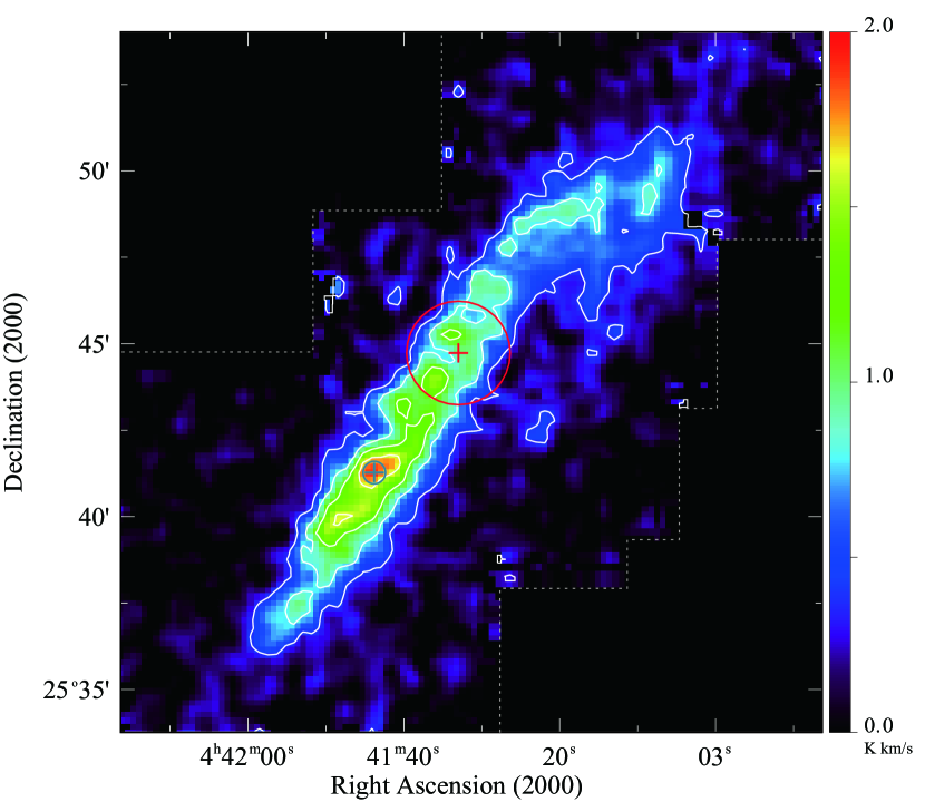
Figure 1: Total integrated intensity map of CCS ($J_{N}=4_{3}-3_{2}$) toward TMC-1. Our target position and the position of OH Zeeman observations (Troland & Crutcher, 2008) are shown in the black and red plus signs, respectively. The sizes of the circles indicate the HPBW beam sizes.

TMC-1 has one of the strongest CCS emission in the Taurus molecular cloud (Suzuki et al., 1992). In figure 1 we show the CCS integrated intensity map of TMC-1. The observed position marked with a black circle in figure 1 is located in the western part of the TMC-1 filament. We observed two molecular lines of CCS ($J_{N}=4_{3}-3_{2}$) and HC₃N ($J=5-4$, 45.490316 GHz, Lafferty & Lovas 1978) simultaneously. The HC₃N line is a non-Zeeman one, and is used to check how well the polarization calibration is performed. In addition, the HC₃N line traces the same density range as the CCS line (Suzuki et al., 1992; Taniguchi et al., 2018). As a backend, we used a newly-developed software spectrometer, PolariS (Mizuno et al., 2014), which has a frequency resolution of 54 Hz (FWHM). The beam size (HPBW) of the Z45 receiver is 40at 45 GHz, which corresponds to 0.024 pc at the location of TMC-1. The typical noise temperature was in the range of 100 $-$ 200 K. The pointing was checked every 1.5 hour with the SiO maser of NML Tau.

We adopted smoothed bandpass calibration (SBC) method (Yamaki et al., 2012) with which we can reduce the integration time of off-source scans by smoothing the spectrum at the off-source blank sky position (the reference position). Since the appropriate spectrum smoothing reduces the noise, we can shorten the integration time for the reference position. The integration time was 120 s and 10 s for the target position and reference position, respectively. We smoothed the spectrum at the reference position using a third-order spline function as the baseline for obtaining the spectrum of molecular lines at the target position. In our Zeeman observations, the SBC method allowed us to reduce the total observation time by a factor of three.

The details of the calibration, beam squint correction, and data analysis will be shown in a forthcoming paper, and some data analysis procedures of the polarization data are summarized in the appendix.

2.2 OTF observations

We also carried out mapping observations of TMC-1 in the on-the-fly (OTF) mode with the Z45 receiver and a digital spectrometer, SAM45 (Kamazaki et al., 2012). The frequency resolution was set to 3.81 kHz, corresponding to the velocity resolution of 0.025 km s^-1. The typical noise temperature was around 100 $-$ 200 K. The pointing was checked every 1.5 hour by observing the SiO maser of NML Tau. The noise level of the map is estimated to be about 0.075 K in a brightness temperature scale using the main beam efficiency of 0.7. CCS ($J_{N}=4_{3}-3_{2}$) and HC₃N ($J=5-4$) lines are simultaneously observed. The map is used to measure the velocity gradient at the observed position. The details of the observations are also described in Dobashi et al. (2019).

3 Results

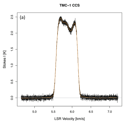
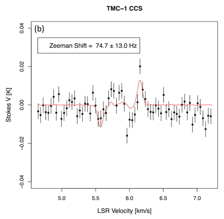
Figure 2: (a) Stokes $I$ profile of CCS toward TMC-1. (b) Stokes $V$ profile of CCS. The red line shows the fitted Stokes $V$ profile. The $t$ and $p$ values of the fitting are $t=9.0$ and $p<2\times 10^{-16}$, respectively.

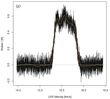
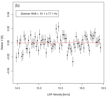
Figure 3: (a) Stokes $I$ profile of the HC₃N ($J=5-4$) satellite component ($F=4-4$) toward TMC-1. Note that the satellite component does not have blended hyperfine components and optically thin. The rest frequency of the HC₃N ($J=5-4,F=5-4$) line was adopted to measure the line-of-sight velocity. (b) Stokes $V$ profile of HC₃N. The red line shows the fitted Stokes V profile. The $t$ and $p$ values of the fitting were $t=0.7$ and $p=0.48$, respectively.

Figures 2 and 3 show the Stokes $I$ and $V$ spectra of the CCS and HC₃N lines toward our observed point, respectively. We applied the beam squint correction to obtain the Stokes $V$ spectra. Our system has a beam squint of the two circularly-polarized components of about 2^′′ mainly in the azimuth direction, with a dependence on the observed elevation. To calculate the splitting, we first fit the observed Stokes $I$ profile with a third-order B-spline function and derive $dI/d\nu$ which is proportional to the Stokes $V$ caused by the Zeeman split as $V\propto dI/d\nu$ (Crutcher et al., 1993). Then, we carried out a least-square fit to the Stokes $V$ spectra with a function of

$${\rm Stokes}\ V=a_{1}+a_{2}I+a_{3}{dI\over d\nu}\ ,$$ (1)

where the coefficients $a_{1}$ and $a_{2}$ are almost zero ($a_{1}\simeq 6.7\times 10^{-3}$ K and $a_{2}\simeq 1.9\times 10^{-3}$). The frequency shift of the Stokes $V$, $a_{3}$, is proportional to the magnetic strength along the line-of-sight direction ($a_{3}\propto B_{\rm los}$), and we derived the frequency shift of $+75.3$ $\pm$ 13.4 Hz, where the second number is the standard error. The $t$ and $p$ values were $t=9.0$ and $p<2\times 10^{-16}$, respectively, suggesting that $a_{3}$ is significantly required to explain the observed Stokes $V$ profile. From this splitting frequency, we derive the line-of-sight magnetic field strength of 117 $\pm$ 21 $\mu$G with the Lande factor of CCS ($J_{N}=4_{3}-3_{2})$ 64 Hz /$100\mu$G (Shinnaga & Yamamoto, 2000). It is worth noting that the CCS line profile can be fitted with 4 Gaussian components with different line-of-sight velocities ($\displaystyle I=\sum_{i=1}^{4}I_{i}$) (Dobashi et al., 2018). Therefore, we implicitly assume that the strength of the magnetic field associated with each component is the same, so that

$$V=\sum_{i=1}^{4}a_{3}{dI_{i}\over d\nu}=a_{3}{dI\over d\nu}\ .$$ (2)

We applied the same procedure as CCS to the HC₃N line simultaneously obtained and derived a frequency shift of $61.1\pm 77.1$ Hz for the satellite component ($F=4-4$). Here, we did not use the main component since it consists of the three optically thick hyperfine components ($F=5-3$, $5-4$, and $6-5$) which make the total profile very complicated. The $t$ and $p$ values of the fitting are $t=0.7$ and $p=0.48$. Thus, the derived frequency shift of HC₃N is statistically insignificant, and we conclude that we detect the CCS Zeeman shift but not for HC₃N. This is the first clear detection of the CCS Zeeman splitting from a prestellar core.

There has been no clear detection reported in previous observations mainly because of the technical difficulties such as low signal-to-noise ratios and instrumental polarization effects. There are at least three advantages in our measurements. Firstly, we used a linear polarization receiver and took a cross-correlation between linearly-polarized components (Heiles et al., 2001), whereas the previous attempts were done with circular polarization reception that can generate significant systematic errors in Stokes $V$ spectra caused by gain inhomogeneity between two-circularly polarized components. Secondly, we applied the SBC method which can improve the signal-to-noise ratio by a factor of about 3 for narrow emission lines within a limited observation time. Lastly, simultaneous observations of the Zeeman line (CCS) and non-Zeeman line (HC₃N) guarantee our detection. In addition, we have done simultaneous observations of CCS and another non-Zeeman line (HC₅N) and obtained the similar splitting of the Stokes $V$ for CCS and no significant splitting for HC₅N. We note that to verify our polarization system, we also observed OMC-2 in $7_{0}-6_{1}A^{+}$ methanol maser line at 44.1 GHz and detected a Zeeman splitting, which was consistent with the previous detection with VLA (Sarma & Momjian, 2011).

4 Importance of magnetic field in TMC-1

How significantly does this magnetic field influence the dynamics of the TMC-1 core? From the Stokes $V$ profiles, we can only derive the line-of-sight strength of the magnetic field. To obtain the true field strength, we need to estimate the field strength on the plane-of-sky. It is, however, difficult to accurately derive the strength of the plane-of-sky component observationally, although we can roughly evaluate the spatially-averaged strength of the plane-of-sky component from linear polarization observations (Crutcher, 2012). From near-infrared polarization observations, the average strength of the plane-of-sky component toward the TMC-1 region is estimated to be $\left<B_{\rm pos}\right>\sim 61\ \mu$ G at the average density of 970 cm^-3 by applying the modified Chandrasekhar-Fermi method (Chapman et al., 2011). The volume density of H₂ at our position is derived to be $3\times 10^{4}$ cm^-3 by applying the LVG method using the CCS ($J_{N}=2_{1}-1_{0}$) and ($J_{N}=4_{3}-3_{2}$) lines (Suzuki et al., 1992). If we scale the above value to the density traced by CCS assuming $B\propto n^{0.5}$, the expected strength is stronger than the line-of-sight component as 339 $\mu$G. We consider that this value of $\left<B_{\rm pos}\right>$ may be significantly overestimated because the TMC-1 core contains multiple components with different velocities and may undergo global contraction which increases the local velocity dispersion.

As mentioned above, at our observed position, the CCS line profile can be fitted with four Gaussian components with different velocities (Dobashi et al., 2018). The four components A, B, C, and D have the centroid velocities of 5.53 km s^-1, 5.69 km s^-1, 5.87 km s^-1, and 5.95 km s^-1, respectively, which are determined by Gaussian fitting of the optically-thin HC₃N isolated hyperfine line (see figure 4(a)). Based on the detailed radiative transfer calculations, the most plausible spatial configurations of these four components are inferred to the one that lines up in order as A, B, C, and D from the furthest position along the line-of-sight (see figure 5), where the components A, B, C, and D are indicated in figure 4(b). The velocity difference of the components A and D is about 0.4 km s^-1, and this may be due to the global infall or converging motion that contributes dominantly to the total line width of the CCS profile ($\approx 0.58$km s^-1). The existence of such a global converging flow is consistent with large-scale velocity gradient seen in wide-field CO maps (Narayanan et al., 2008). Such a global motion is likely to significantly contribute to the total velocity width in this core. Thus, the magnetic strength estimated by the Chandrasekhar-Fermi analysis may be overestimated. The individual components have the velocity widths of about 0.2 km s^-1, about a third of the total velocity width. Therefore, the strength of the plane-of-sky component may be much weaker as 20 $\mu$G at 970 cm^-3. Assuming that the field strength increases in proportion to the square root of the number density, $\left<B_{\rm pos}\right>$ of TMC-1 at $n\simeq 3\times 10^{4}$ cm^-3 is scaled to be $\left<B_{\rm pos}\right>\simeq 100\ \mu$G. The total magnetic field strength at our observed position can be evaluated to be $B_{\rm tot}\equiv\sqrt{B_{\rm los}^{2}+\left<B_{\rm pos}\right>^{2}}\sim 154\ \mu$G with an inclination angle of $\sim$45^∘ with respect to the line-of-sight. This value is comparable to the one derived from our Zeeman measurements.

Dynamical evolution of a magnetized core is determined by a dimensionless parameter called a normalized mass-to-magnetic-flux ratio (Crutcher, 2012).

$$\lambda\equiv{(M_{\rm core}/\Psi_{B})\over(M_{\rm core}/\Psi_{B})_{\rm cr}}={(N_{\rm H_{2}}/B)\over(N_{\rm H_{2}}/B)_{\rm cr}}\ ,$$ (3)

where $N_{\rm H_{2}}$ is the column density of hydrogen molecules, $M_{\rm core}$ is the core mass, $\Psi_{B}$ is the magnetic flux, $(M_{\rm core}/\Psi_{B})_{\rm cr}$ is the critical mass-to-flux ratio of $7.6\times 10^{-21}N_{\rm H_{2}}/B$ (Nakano, 1978). If $\lambda\geq 1$, the magnetic field is too weak to support the core against its contraction. Such a core is called magnetically supercritical, and can continue to gravitational contraction to form stars. On the other hand, if $\lambda<1$, the core is called magnetically subcritical. In interstellar space, such a core can continue gravitational contraction by losing its magnetic flux due to ambipolar diffusion. The timescale of the gravitational contraction is at least an order of magnitude longer than that of the former in the absence of strong turbulence (Nakamura & Li, 2008), and thus the resultant efficiency of star formation becomes very different from the former.

From our derived field strength, the mass-to-flux ratio of TMC-1 is estimated to be $\lambda\simeq 2.2$, where we used the H₂ column density of $3\times 10^{22}$ cm^-2 from the Herschel data (Malinen et al., 2012). Thus, TMC-1 is likely to have a moderately-strong supercritical magnetic field. Such a magnetic field can remove the core angular momentum efficiently through the magnetic braking, but cannot prevent from the gravitational contraction completely.

Our measurement is consistent with the results of the previous OH Zeeman observations (Troland & Crutcher, 2008) toward the position with about 5^′ offset along the filament from our position (see figure 1), corresponding to about 0.2 pc offset. From the OH Zeeman observations, the field strength is derived to be $B_{\rm los}\simeq$ 14 $\mu$G at $n_{\rm H_{2}}=5000$ cm^-3. If the field strength increases as $B_{\rm los}\propto n_{\rm H_{2}}^{2/3}$ (the weak field case), the line-of-sight field strength is evaluated to be 46 $\mu$G, corresponding to $B_{\rm tot}\simeq 110\ \mu$G when we adopt $\left<B_{\rm pos}\right>\simeq$ 100 $\mu$G with an inclination angle of $\sim$ 30^∘. The flux-to-mass ratio at the OH position is estimated to be $\lambda\simeq 3$, where we adopt a column density of $2\times 10^{22}$ cm^-2 (Malinen et al., 2012). Thus, the OH position is magnetically supercritical, similarly to our position.

The infall velocity at our position is inferred to be $\sim$ 0.6 km s^-1, about three times the sound speed for $T=10$ K, assuming that the infall proceeds along the magnetic field lines with an inclination angle of $\sim$ 45^∘. This infall velocity is in agreement with the terminal velocity of isothermal collapse of spherical and cylindrical clouds (Larson, 1969; Nakamura, 1998; Ogino et al., 1999). Thus, we suggest that the TMC-1 filament is now dynamically contracting toward the center and on the verge of protostellar formation. The dense cores distributed along the TMC-1 filament might be in the evolutionary stages just before the formation of the first hydrostatic core.

5 Summary

• We performed the CCS ($J_{N}=4_{3}-3_{2}$) Zeeman observations toward the TMC-1 using the Nobeyama 45-m telescope and detected the significant splitting of 74.7 $\pm$ 13.0 Hz. We estimated the line-of-sight magnetic strength to be 110 $\mu$G $\pm$ 21 $\mu$G.

• We also simultaneously observed a non-Zeeman line, HC₃N to check how well the polarization calibration was perfomed, and we did not detect any significant shift in the Stokes $V$ profile. This non-detection of the HC₃N Zeeman shift supports our detection of the CCS Zeeman shift.

• Using the H₂ column density measurements by Herschel observations, we estimated the normalized mass-to-magnetic flux ratio of 2.2, assuming the inclination angle of 45^∘. The inclination angle is inferred from the comparison with the results of the near infrared linear polarization observations. We conclude that the TMC-1 is magnetically supercritical.

• We recently suggested the TMC-1 infalling radially toward the filament axis by solving the detailed one-dimensional radiative transfer (Dobashi et al., 2018). This is consistent with our conclusion that the TMC-1 is magnetically supercritical.

This work is supported in part by a Grant-in-Aid for Scientific Research of Japan (24244017). We thank Satoshi Yamamoto and Ryohei Kawabe for valuable comments, suggestions, and encouragements. We are grateful to Hideo Ogawa, Kimihiko Kimura, Yoshinori Yonekura, Shuro Takano, Daisuke Iono, Nario Kuno, Munetake Momose, Nozomi Okada, Minato Kozu, Yutaka Hasegawa, Kazuki Tokuda, Tetsu Ochiai, Taku Nakajima, and Hiroko Shinnaga for their contribution to developing the polarization system and valuable comments. We are grateful to the staffs at the Nobeyama Radio Observatory (NRO) for operating the 45-m. NRO is a branch of the National Astronomical Observatory, National Institutes of Natural Sciences, Japan.

Appendix A Polarimetry

Spectroscopic polarimetry is carried out using the dual linear polarization capability of the Z45 (Nakamura et al., 2015) receiver and the PolariS spectrometer (Mizuno et al., 2014). PolariS is a polarization spectrometer that accepts four IF signals ($X_{0}$, $X_{1}$, $Y_{0}$, and $Y_{1}$; $X$ and $Y$ stand for linear polarization components and suffice for two spectral windows) with a 4-MHz bandwidth for each and produce four power spectra of $\left<X_{0}X^{*}_{0}\right>$, $\left<X_{1}X^{*}_{1}\right>$, $\left<Y_{0}Y^{*}_{0}\right>$, and $\left<Y_{1}Y^{*}_{1}\right>$ and two cross-power spectra of $\left<X_{0}Y^{*}_{0}\right>$, $\left<X_{1}Y^{*}_{1}\right>$. We assigned line species of CCS and HC₃N in the spectral windows of 0 and 1, respectively. Stokes parameters are derived by using outputs from PolariS as

$$\left(\begin{array}[]{c}\frac{\left<XX^{*}\right>}{G_{X}G^{*}_{X}}\\ {\left<XY^{*}\right>\over G_{X}G^{*}_{Y}}\\ {\left<X^{*}Y\right>\over G_{Y}G^{*}_{X}}\\ {\left<YY^{*}\right>\over G_{Y}G^{*}_{Y}}\end{array}\right)=\frac{1}{2}\left(\begin{array}[]{cccc}1&D^{*}_{X}&D_{X}&D_{X}D^{*}_{X}\\ D^{*}_{Y}&1&D_{X}D^{*}_{Y}&D_{X}\\ D_{Y}&D_{Y}D^{*}_{X}&1&D^{*}_{X}\\ D_{Y}D^{*}_{Y}&D_{Y}&D^{*}_{Y}&1\end{array}\right)\left(\begin{array}[]{cccc}1&\cos 2\psi&\sin 2\psi&0\\ 0&-\sin 2\psi&\cos 2\psi&i\\ 0&-\sin 2\psi&\cos 2\psi&-i\\ 1&-\cos 2\psi&-\sin 2\psi&0\end{array}\right)\left(\begin{array}[]{c}I\\ Q\\ U\\ V\end{array}\right).$$ (20)

Here $\psi$ is the position angle of the $X$-polarization feed projected on the celestial sphere. With the Nasmyth optics of the Nobeyama 45-m telescope, it is given by $\psi=\phi_{\rm PA}+\phi_{\rm EL}$, where $\phi_{\rm PA}$ and $\phi_{\rm EL}$ are parallactic angle and elevation angle, respectively. The first matrix in equation (20) is composed by D-terms, which indicates cross talk coefficients between $X$ and $Y$. The voltage-based complex gain is described as $G_{X}$ and $G_{Y}$. The argument of $G_{Y}$ indicates relative phase between $X$ and $Y$ polarizations.

We address Stokes $V$ which responses the Zeeman split. When the source is not linearly polarized (i.e. $Q=U=0$), we have

$${\left<XY^{*}\right>\over G_{X}G^{*}_{Y}}=(D_{X}+D^{*}_{Y})I+i(1-D_{X}D^{*}_{Y})V.$$ (21)

The instrumental phase offset between $X$ and $Y$ polarizations, measured using the wire grid and the P-cal signal (see Section 2), is stored in $G_{Y}$. This $X$-$Y$ phase calibration is verified by non-detection of Stokes $V$ toward the Crab nebula.

Appendix B Gain and phase calibration

The amplitudes of gains can be determined by applying system noise temperature, $T_{\rm sys}$ as

$$|G|={1\over\sqrt{2k_{B}T_{\rm sys}}}\ ,$$ (22)

where $k_{B}$ is the Boltzman constant. We used the digital measuring method (Nakatake et al., 2010) using level histograms of the digitizer in the PolariS. Because Stokes $V$ component is given by the imaginary part of $\left<XY^{*}\right>$, it is crucial to calibrate the phase of $G_{Y}$, with respect to that of $G_{X}$. We employed three ways of $G_{Y}$ phase calibration; a linearly polarized calibrator source, wire grid, and phase-calibration (P-cal) signal. We used the Crab nebula as the linearly polarized calibrator source whose polarization angle is $151^{\circ}.0$ at 31 GHz (Cartwright et al., 2005) or $152^{\circ}.1\pm 0^{\circ}.3$ at 90 GHz. To determine the orientation of $X$ and $Y$ feed projected on the sky, we observed the Crab nebula before and after the meridian at the different parallactic angles. In addition, we inserted a wire grid in front of the receiver feed to input linearly polarized signals. While signals from the sky transmit through the wire grid, the reflected signals originate from the ambient load (i.e. an absorber at the room temperature). The contrast between the temperatures of the ambient load and the sky yields linearly polarized continuum signals. Cross correlation of $\left<XY^{*}\right>$ while inserting the wire grid allows us to calibrate $XY$ delay and phase. The wire grid was inserted during antenna slew before calibrator scans. To verify time stability of $XY$ phase, we also injected a phase calibration signal (P-cal) which is a linearly polarized monochromatic wave at the frequency beside the CCS emission. We solve 180-degree ambiguity in phase of P-cal by comparing with cross correlation toward the Crab nebula.

We measured the delay and phase offsets between $X$ and $Y$ signal paths by taking cross correlation, $\left<XY^{*}\right>$, when we inserted a wire grid in front of the feed horn (see figure 12 in Nakamura et al. (2015)). The reflection and transmission waves at the wire grid terminate onto the ambient load and the sky, respectively. Thus, the amplitude of the normalized cross correlation coefficient is $(T_{\rm amb}-T_{\rm sky})/\sqrt{(T_{\rm RX}+T_{\rm sky})(T_{\rm RX}+T_{\rm amb})}$, and the phase, $\phi=\phi_{XY}+2\pi\tau_{XY}\nu_{BB}$, where $\phi_{XY}$ and $\tau_{XY}$ are phase and delay offsets between $X$ and $Y$ signal paths, respectively.

Appendix C D-term correction

The cross polarization leakage (D-term) is determined by using both unpolarized calibrators and linearly polarized calibrator, respectively. We used the Venus or Jupiter as the unpolarized calibrator. We assume that Stokes $Q=U=V=0$ for the unpolarized calibrator, then the cross correlation will be $\left<XY^{*}\right>/G_{X}G^{*}_{Y}=(D_{X}+D^{*}_{Y})I$. Giving the model Stokes $I$ (antenna temperature) of the calibrator, we determine the value of $D_{X}+D^{*}_{Y}$ and apply it to equation (21).

Appendix D Beam squint

Although we employed dual linear polarization feeds, we focus on Stokes $V$ which is proportional to the difference between circular polarizations (RHCP and LHCP). The optics of the antenna and the receiving system may have differences in beam patterns between RHCP and LHCP. The inhomogeneity in circular polarization can cause false Stokes $V$, and then produce fake Zeeman-split-like features when the source has a velocity gradient. The fake Zeeman shift, $\Delta v$, is given by

$$\Delta v=\left(\begin{array}[]{c}\frac{dv}{d\alpha}\\ \frac{dv}{d\delta}\end{array}\right)\left(\begin{array}[]{cc}\cos{\rm\phi_{\rm PA}}&\sin{\rm\phi_{\rm PA}}\\ -\sin{\rm\phi_{\rm PA}}&\cos{\rm\phi_{\rm PA}}\end{array}\right)\left(\begin{array}[]{c}\theta_{\rm AZ}\\ \theta_{\rm EL}\end{array}\right),$$ (29)

where $\frac{dv}{d\alpha}$ and $\frac{dv}{d\delta}$ are the velocity gradients, $\phi_{\rm PA}$ is the parallactic angle, and $(\theta_{\rm AZ},\theta_{\rm EL})$ is the beam squint between RHCP and LHCP. We measured the beam squint by observing CH₃OH maser (44.1 GHz) emission toward the OMC-2 (Sarma & Momjian, 2011; Momjian & Sarma, 2012). The maser source is so compact that we presume the identical positions of RHCP and LHCP emissions. Cross scans towards the maser yields the beam squint of $(\theta_{\rm AZ},\theta_{\rm EL})\simeq(-2^{\prime\prime}.08\pm 0^{\prime\prime}.30,-0^{\prime\prime}.24\pm 0^{\prime\prime}.30)$.

More accurately, the beam squint has a dependence on the elevation of the observations. Figure 6 indicates the beam squint measured with the SiO maser line toward NML Tau as a function of the observed elevation. We fit the beam squint of ($dAZ,dEL$) as

$$dAZ = dAZ_{0}+dAZ_{1}\cos EL+dEL_{1}\sin EL$$ (30)

$$dEL = dEL_{0}-dAZ_{1}\sin EL+dEL_{1}\cos EL$$ (31)

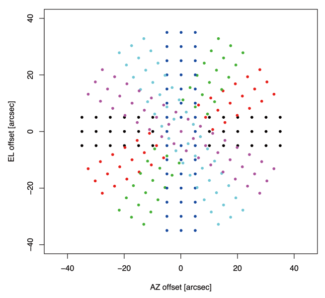
Figure 7: Scan pattern of the beam-squint measurement toward the NML Tau SiO maser. Rectangular 15 $\times$ 3 grid spaced by 5(i.e., 70$\times$ 10) excursions are rotated by 30^∘ step to cover a 35-radius circle centering the SiO maser.

where $dAZ_{0}=-0^{\prime\prime}.41\pm 0^{\prime\prime}.16$, $dEL_{0}=-1^{\prime\prime}.25\pm 0^{\prime\prime}.16$, $dAZ_{1}=-2^{\prime\prime}.05\pm 0^{\prime\prime}.15$, and $dEL_{1}=-0^{\prime\prime}.39\pm 0^{\prime\prime}.16$. towards rectangular mapping towards the SiO maser source NML Tau. The scan pattern is presented in figure 7. We applied correction in the calibration process of the beam squint using the above fitting formula.

We also measured the velocity gradient of CCS and HC₃N emission by analyzing mean velocity (moment-1) map of the TMC-1 molecular cloud. We cropped the field where the signal-to-noise ratio of the integrated intensity (moment-0 map) exceeds $2\sigma$ of the standard deviation of emission-free area. The velocity gradients of CCS and HC₃N were given as $(3.68,3.43)$ km s^-1 deg^-1 and $(3.63,2.74)$ km s^-1 deg^-1, respectively. Then every Stokes $V$ spectrum was corrected by applying the beam squint and the velocity gradient.

Appendix E Four components of CCS

The CCS line profile at our observed position appears to have multiple components with different line-of-sight velocities [see Dobashi et al.(2018) for more accurate and detail analysis]. The CCS emission is relatively strong and therefore emission from components in the back can be absorbed by molecules in the foreground components. Applying radiative transfer calculations, we can infer the spatial configuration of the multiple components along line-of-sight.

We observed CCS ($J_{N}=4_{3}-3_{2}$) and HC₃N ($J=5-4$) lines simultaneously. The HC₃N ($J=5-4$) line has multiple hyperfine structure. Two hyperfine lines of $F=5-5$ and $F=4-4$ are weak and are isolated from other hyperfine lines ($F=4-3$, $F=5-4$, $F=6-5$). Thus, intrinsic line intensities of these hyperfine lines are likely to be optically thin. Since HC₃N ($J=5-4$) has a critical density comparable to that of CCS ($J_{N}=4_{3}-3_{2}$), we consider that they trace molecular gas with a similar density range.

First, we fit the HC₃N ($J=5-4$, $F=5-5$ and $F=4-4$) with $n$ Gaussian components. Each component has three free parameters: the peak intensity, centroid velocity, and velocity dispersion. In other words, we have $3n$ free parameters. We fit the line profile in the range of $V_{\rm LSR}=5.2-6.2$ km s^-1 applying the $\chi^{2}$ test by increasing the number of $n$. The reduced $\chi^{2}$ of the fit obtained $\chi_{r}^{2}$=2.6543, 1.0896, 1.0016, and 1.0013 for $N=2,3$, 4, and 5, respectively. The $\chi^{2}_{r}$ value becomes almost $\chi^{2}_{r}\simeq 1$ for $N\geq 4$. In addition, for $N\geq 5$, the Gaussian components tend to fit the noises in the spectral line profile. Thus, we found that the line profile is fitted with $N=4$ Gaussian components, and we call these components A–D in the order of the best fitting centroid velocities. We show the results of the fitting in figure 4(a).

Next, we fit the CCS line profile with 4 components with the same centroid velocities as we obtained from HC₃N. We assume that the optical depth of each component has a Gaussian shape.

$$\tau_{i}(v)=\tau^{0}_{i}\exp\left[-{1\over 2}\left({v-v_{i}\over\sigma_{i}}\right)^{2}\right]\ ,$$ (32)

where $\tau_{i}^{0}$, $v_{i}$, and $\sigma_{i}$ are the optical depth at the line center, centroid velocity, and the velocity dispersion of the $i$-th component, respectively. The intrinsic emission of the $i$-th component, $T_{i}$, before being absorbed by the foreground gas is expressed as

$$T_{i}(v)=T_{i}^{0}[1-\exp(-\tau_{i}(v))]\ ,$$ (33)

where $T_{i}^{0}$ is the intensity at the line center for $\tau_{i}^{0}\gg 1$. If we assume that all of the four components are lying on the same line-of-sight in the order of $i=1,2,3$, and 4 having the $i=1$ component to be the furthest from the observer, the total emission we should observe is then given as

$$T=\sum_{i=1}^{4}T_{i}[1-\exp(-S_{i}(v))]\ ,$$ (34)

where

$$S_{i}(v)=\left\{\begin{array}[]{ll}\sum_{j=i+1}^{4}\tau_{j}(v)&(i=1,2,3)\\ 0&(i=4)\end{array}\right.\ .$$ (35)

We fit the CCS line profile with the above computed total emission, $T$. In total, we have $4!=24$ possible spatial configurations of the four components A–D to assign $i=1$ (the furthest) to $i=4$ (the nearest, see figure 5). Each configuration has $3\times 4=12$ free parameters ($\tau_{i}^{0}$ and $\sigma_{i}$ in Equation (A7) and $T_{i}^{0}$ in Equation (A8)). Applying the $\chi^{2}$ test, we found the most plausible spatial configuration is (A, B, C, and D) from the furthest position along the line-of-sight giving a reduced $\chi^{2}$ of $\sim 1.06$. The results of the $\chi^{2}$ test are summarized in Table 1. We show the fitted spectrum in figure 4(b). We also summarized the fitting parameters in Table 2. Though the true configuration of the four velocity components may not be as simple as in our model, we would interpret the results of the radiative transfer calculations as the global motion of contraction.

Dobashi et al. (2018) conducted essentially the same calculations as above including the HC₃N ($J=4-3$, $F=5-4$ and $F=6-5$) main components which are optically thicker than the CCS line. Therefore, the spatial configuration is more distinguishable due to stronger absorption effects. Their result agrees well with that of CCS. Thus, we concluded that the most plausible spatial configuration is (A, B, C, and D) from the furthest position along the line-of-sight.

Appendix F Stokes $I$ and $V$ spectra for the main component of HC₃N

For confirmation, we applied the same procedure as used for the CCS analysis to the main component of HC₃N. The Stokes $I$ and $V$ profiles are shown in figure 8. The main component of HC₃N consists of three hyperfine components. The TMC-1 position contains 4 components with different velocities and thus 12 components are blended for HC₃N. The 4 components may have different optical depths and different line-of-sight velocity gradients. These effects are likely to cause the different beam squints, and presumably sometimes significantly influence the derived Stokes $V$ pattern when the velocity gradients of blended components are very different.

Therefore, for the verification of our polarization calibration, we used a satellite line, which does not contain different hyperfine components. We note that the $\chi^{2}$ test for the fitting of the main components shows no statistically-significant shift, and thus we can conclude that our polarization calibration is reasonably accurate even for the main components. However, we recommend to use relatively-strong non-Zeeman emission lines, which do not contain blended hyperfine lines, for the similar verification of the polarization calibration. For the measurements toward other positions, this effect was likely to generate artificial patterns in the derived Stokes $V$ profiles for the main component.

Table 1: The reduced $\chi^{2}$ value for the different configurations

The reduced $\chi^{2}$ value for the different configurations Configuration $\chi^{2}_{r}$ ABCD 1.060 ABDC 1.114 ACBD 1.124 ACDB 1.147 ADBC 1.104 ADCB 1.081 BACD 1.085 BADC 1.157 BCAD 1.085 BCDA 1.085 BDAC 1.157 BDCA 1.157 CABD 1.127 CADB 1.147 CBAD 1.097 CBDA 1.097 CDAB 1.147 CDBA 1.102 DABC 1.105 DACB 1.081 DBAC 1.161 DBCA 1.161 DCAB 1.081 DCBA 1.102

Table 2: The fitted parameters for the CCS ($J_{N}=4_{3}-3_{2}$) Line

The fitted parameters for the CCS ($J_{N}=4_{3}-3_{2}$) Line Component Peak Intensity ($T_{i}^{0}$) Velocity Dispersion ($\sigma_{i}$) $\tau_{i}^{0}$ $T_{\rm ex}$ (K) (km s^-1) (K) A 2.22 $\pm$ 0.04 0.052 $\pm$ 0.001 2.15 $\pm$0.07 6.0 $\pm$0.1 B 3.17 $\pm$ 0.07 0.116$\pm$ 0.001 1.37 $\pm$ 0.07 7.3$\pm$ 0.2 C 2.20 $\pm$ 0.01 0.070 $\pm$0.002 1.88 $\pm$ 0.10 5.9$\pm$ 0.1 D 2.79 $\pm$ 0.03 0.047 $\pm$0.001 1.08 $\pm$ 0.05 6.8$\pm$ 0.1

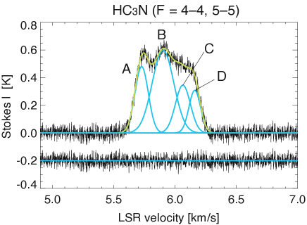
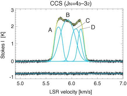
Figure 4: (left) A hyperfine component of the HC₃N ($J=5-4$) line fitted with four Gaussian profiles (blue lines). The yellow line denotes their simple sum. The $F=5-5$ and $F=4-4$ profiles are combined to improve the noise level. The residual spectrum of the Gaussian fitting is shown just below the actual spectrum. (right) CCS line profile fitted with four components. The blue lines are the simple Gaussian functions, and the yellow line represents their sum calculated taking into account the radiative transfer (see Dobashi et al. 2018).

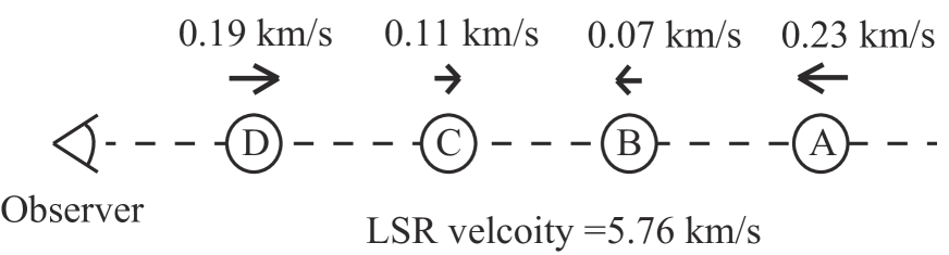
Figure 5: Spatial configuration of the four CCS components. The velocities indicated by the arrows are the relative velocities with respect to the mean velocity of 5.76 km s^-1.

Figure 6: The beam squint measured with the SiO maser line from NML Tau as a function of the observed elevation. The fitted functions are shown in the upper right.

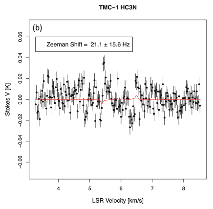
Figure 8: Same as figure 3 but for the HC₃N ($J=5-4$) main component ($F=6-5,5-4,4-3$) toward TMC-1. The three hyperfine components are blended for the main component, and thus the main line consists of 12 components since 4 components with different velocities are blended at the observed position. (b) The Stokes $V$ profile of the main component of HC₃N. The red line shows the fitted Stokes V profile. The $t$ and $p$ values of the fitting were $t=0.7$ and $p=0.48$, respectively.

References

- Aumont et al. (2010) Aumont, J., Conversi, L., Thum, C., et al. 2010, A&A, 514, A70
- Benson & Myers (1989) Benson, P. J. & Myers, P. C. 1989, ApJS, 71, 89
- Bergin & Tafalla (2007) Bergin, E. A., & Tafalla, M. 2007, ARA&A, 45, 339
- Cartwright et al. (2005) Cartwright, J. K., Pearson, T. J., Readhead, A. C. S., et al. 2005, ApJ, 623, 11
- Chapman et al. (2011) Chapman, N. L., Goldsmith, P. F., Pineda, J. L. et al. 2011, ApJ, 741, 21
- Crutcher (2012) Crutcher, R. M. 2012, ARAA, 50, 29
- Crutcher et al. (1993) Crutcher, R. M., Troland, T., H., & Goodman, A. A., 1993, ApJ, 407, 175
- Dobashi et al. (2018) Dobashi, K., Shimoikura, T., Nakamura, F. et al., 2018, ApJ, 864, 82
- Dobashi et al. (2019) Dobashi, K., Shimoikura, T., Ochiai, T., F. et al., 2019, ApJ, 879, 88
- Feher et al. (2016) Fehér, O., L. V. Tóth, L. V., Ward-Thompson, D., et al. 2016, A&A, 590, A75
- Fiebig & Guesten (1989) Fiebig, D. & Guesten, R. 1989, A&A, 214, 333
- Heiles et al. (2001) Heiles, C., Perillat, P., Nolan, M., et al. 2001, PASP, 113, 1247
- Kamazaki et al. (2012) Kamazaki, T., et al., 2012, PASJ, 64, 29
- Lafferty & Lovas (1978) Lafferty, W. J. & Lovas, F. J., 1978, JPCRD, 7, L441
- Larson (1969) Larson, R. 1969, MNRAS, 145, 271
- Levin et al. (2001) Levin, S. M., Langer, W. D., Velusamy, T., et al. 2001, ApJ, 555, 850
- Li et al. (2014) Li, H.-B., Goodman, A., Sridharan, T. K., et al. 2014, Protostars and Planets VI, Henrik Beuther, Ralf S. Klessen, Cornelis P. Dullemond, and Thomas Henning (eds.), University of Arizona Press, Tucson, p. 101
- Li et al. (2004) Li, Z.-Y., & Nakamura, F. 2004, ApJ, 609, L83
- Li et al. (2014) Li, Z.-Y., Banerjee, R., Pudritz, R. E. et al. 2014, Protostars and Planets VI, Henrik Beuther, Ralf S. Klessen, Cornelis P. Dullemond, and Thomas Henning (eds.), University of Arizona Press, Tucson, p.173
- Malinen et al. (2012) Malinen, J., Juvela, M., Rawlings, M. G., 2012, A&A, 544, A50
- Marka et al. (2012) Marka, C., Schreyer, K., Launhardt, R., Semenov, D. A., Henning, Th. 2012, A&A, 537, 4
- Mizuno et al. (2014) Mizuno, I., Kameno, S., Kano, A. 2014, JAI, 3, 1450010
- Momjian & Sarma (2012) Momjian, E., & Sarma, A. P. 2012, AJ, 144, 189
- Mouschovias & Tassi (2009) Mouschovias, T. & Tassis, K. 2009, MNRAS, 400, 15
- Nakano (1978) Nakano, T. & Nakamura, T. 1978, PASJ, 30, 681
- Nakamura (1998) Nakamura, F. 1998, ApJL, 507, L165
- Nakamura & Li (2008) Nakamura, F. & Li. Z.-Y., 2008, ApJ, 687, 354
- Nakamura et al. (2014) Nakamura, F., Sugitani, K., Tanaka, T., et al., 2014, ApJ, 791, L23
- Nakamura et al. (2015) Nakamura, F., Ogawa, H., Yonekura, Y. et al. 2015, PASJ, 67, 117
- Nakatake et al. (2010) Nakatake, A., Kameno, S., & Takeda, K. 2010, PASJ, 62, 1361
- Narayanan et al. (2008) Narayanan, G., Heyer, M. H., Brunt, C. et all, 2008, ApJ, 177, 341
- Ogino et al. (1999) Ogino, S., Tomisaka, K., & Nakamura, F.. 1999, PASJ, 51, 637
- Sarma & Momjian (2011) Sarma, A. P., & Momjian, E. 2011, ApJ, 730, L5
- Shimoikura et al. (2018) Shimoikura, T., Dobashi, K., Nakamura, F., Matsumoto, T., Hirota, T. 2018, ApJ, 885, 45
- Shimoikura et al. (2019) Shimoikura, T., Dobashi, K., Nakamura, F., Shimajiri, Y., Sugitani, K. 2019, PASJ, in press (arXiv:1809.09855)
- Shinnaga & Yamamoto (2000) Shinnaga, H., & Yamatomo, S., 2000, ApJ, 544, 330
- Shinnaga et al. (1999) Shinnaga, H., Tsuboi, M., Kasuga, T. 1999, in Star Formation 1999, ed. T. Nakamoto, Nobeyama Radio Observatory, p.175
- Shu et al. (1989) Shu, F. H., Adams, F. C., & Lizano, S. 1987, ARAA, 25, 23
- Suzuki et al. (1992) Suzuki, H., Yamatomo, S., Ohishi, M., et al. 1992, ApJ, 392, 551
- Taniguchi et al. (2018) Taniguchi, K., et al. 2018, ApJ, 866, 32
- Torres et al. (2007) Torres, R. M., Loinard, L., Mioduszewski, A. J., Rodríguez, L. F., 2007, ApJ, 671, 1813
- Troland & Crutcher (2008) Troland, T. H., & Crutcher, R. M. 2008, ApJ, 680, 457
- Turner & Heiles (2006) Turner, B. E., & Heiles, C., 2006, ApJS, 162, 388
- Yamaki et al. (2012) Yamaki, H., Kameno, S., Beppu, H., et al. 2012, PASJ, 64, 118
- Yamamoto et al. (1990) Yamamoto, S., et al. 1990, ApJ, 361, 318
- Zhao et al. (2016) Zhao, B., et al. 2016, MNRAS, 460, 2050