Radio Pulsar Sub-Populations (I) :
The Curious Case of Nulling Pulsars

Abstract

About $\sim$200 radio pulsars have been observed to exhibit nulling episodes - short and long. We find that the nulling fraction of a pulsar does not have any obvious correlation with any of the intrinsic pulsar parameters. It also appears that the phenomenon of nulling may be preferentially experienced by pulsars with emission coming predominantly from the polar cap region, and also having extremely curved magnetic fields.

sushan@ncra.tifr.res.in

12.3456/s78910-011-012-3 #### 000 0000 1– 1

1 Introduction

Fifty years of observations have yielded $\sim$3000 neutron stars, with diverse characteristic properties, which fall into three major categories, namely - a) the rotation powered, b) the accretion powered, and c) the internal-energy powered neutron stars; according to their mechanisms of energy generation [Kaspi (2010), Konar (2013), Konar et al. (2016), Konar (2017)]. Radio pulsars, which belong to the category of rotation powered pulsars (RPP), are strongly magnetized rotating neutron stars (mostly isolated or in non-interacting binaries) characterized by their short spin periods ($P\sim 10^{-3}-10^{2}$ s) and large inferred surface magnetic fields ($B\sim 10^{8}-10^{15}$ G). Powered by the loss of rotational energy, they emit highly coherent radiation (typically spanning almost the entire electromagnetic spectrum) which are observed as narrow emission pulses. The abrupt cessation of this pulsed emission for several pulse periods, observed in a small subset of radio pulsars, is known as the phenomenon of nulling - noticed for the first time by ?). Since then, close to two hundred radio pulsars have been observed to experience nulling. In this context, it needs to be noted that most of the $\sim$2600 radio pulsars are neither monitored regularly, nor are searched for the presence of nulling. This would imply that two hundred is just a lower limit to the actual number of nulling pulsars. On the other hand, presence of nulling may also depend on the sensitivity of a given telescope (e.g. a telescope with a low sensitivity may consider a pulsar to be nulling when a similar (or same) pulsar might be detected in weak emission by an instrument with higher sensitivity), giving rise to an over-estimate of the number of nulling pulsars.

In general, two parameters are used to quantify the phenomenon of nulling –

1. the nulling fraction (NF) - the total percentage fraction of pulses without detectable emission; and,

2. the null length (NL) - the duration of a given nulling episode.

Both NF and NL are observed to span a wide range - while NF ranges from just a few to more than 90%, NL can go from the simple case of single pulse nulls to the extreme situation of complete disappearance of pulsed emission for as long as a few years. Even though most pulsars are known to be characterised by a single value of NF (see the tables in A for some contrary cases), neither NF nor NL can uniquely describe the behaviour of a nulling pulsar. It is well known that NL not only varies from one pulsar to another, but also from episode to episode for a given pulsar [Young et al. (2012)]. Moreover with increasing data it is becoming evident that two different pulsars having very different values of NL and totally different nulling behaviour can have the same average value of NF [Gajjar et al. (2012)]. For example, the long quiescent states of intermittent pulsars are in stark contrast to the longest known quiescence times of ordinary nulling pulsars, i.e., they differ in their nulling timescale by about five orders of magnitude - even when the NF values are similar for both cases.

A detailed discussion on different types of nulling behaviour can be found in Gajjar (?) and references therein. Despite the wide variation in NL, the population does render itself to a broad classification, depending on the nature of nulling, as follows -

1. Classical Nuller (CN) - pulsars with mostly single (or just a few) pulse nulls, for example - J0837-4135, J2022+5154 [Gajjar et al. (2012)];

2. Intermittent Nuller (IN) - NL is longer, could be up-to a few hours combined with a longer period of activity, for example - J1717-4054 [Johnston et al. (1992)], J1634-5107 [O’Brien et al. (2006)], J1709-1640 [Naidu et al. (2018)];

3. Intermittent Pulsar (IP) - NL can vary from days to years, for example - J1933+2421 [Kramer et al. (2006a)], J1832+0029 [Lorimer et al. (2012)], J1910+0517 & J1929+1357 [Lyne et al. (2017)];

4. Rotating Radio Transient (RRAT) - Discovered in 2006, the RRATs are characterised by their sporadic single pulse emissions [McLaughlin et al. (2006)]. Whether these can be considered to be part of the nulling fraternity is a contentious issue, which we plan to take up in a later study [Konar (2019)].

The phenomenon of nulling is usually observed to be associated with other emission features, like the drifting of sub-pulses and mode changing [Wang et al. (2007)]. Certain other behavioural changes have also been seen in nulling pulsars. In J1933+2421 the spin-down rate has been observed to decrease in the inactive phase compared to the active phase, suggestive of a depletion in the magnetospheric particle outflow in the quiescent phase of the pulsar [Kramer et al. (2006b), Lyne et al. (2009)]. An exponential decrease in the pulse energy during a burst has also been seen in certain nulling pulsars [Rankin & Wright (2008), Bhattacharyya et al. (2010), Li et al. (2012), Gajjar et al. (2014)]. Interestingly, nulling behaviour has not yet been observed in a millisecond pulsar [Rajwade et al. (2014)], even though the cumulative study of this class of pulsars is close to $10^{3}$ years.

In general, two different classes of models are invoked to explain the phenomenon of nulling, explaining it to arise from - a) intrinsic causes or b) geometrical effects. Some of the models attributing nulling to an intrinsic cause are as follows -

• the loss of coherence conditions [Filippenko & Radhakrishnan (1982)];

• a complete cessation of primary particle production [Kramer et al. (2006b), Gajjar et al. (2014)];

• changes in the current flow conditions in the magnetosphere [Timokhin (2010)];

• a transition to a much weaker emission mode (or an extreme case of mode changing) [Esamdin et al. (2005), Wang et al. (2007), Timokhin (2010), Young et al. (2014)];

• time-dependent variations in an emission ‘carousel model’ [Deshpande & Rankin (2001), Rankin & Wright (2007)]; etc.

On the other hand, a variety of geometrical effects have also been suggested to explain nulling, like -

• the line-of-sight passing between emitting sub-beams giving rise to ‘pseudo-nulls’ [Herfindal & Rankin (2007), Herfindal & Rankin (2009), Rankin & Wright (2008)];

• occurrence of various unfavourable changes in the emission geometry [Dyks et al. (2005), Zhang et al. (2007)].

Detailed investigations of the nulling behaviour of individual pulsars and theoretical modeling of this phenomenon have been undertaken by many groups [Ritchings (1976), Rankin (1986), Biggs (1992), Wang et al. (2007), Gajjar et al. (2012)]. In many instances, nulling has been observed across a wide frequency range making it a broadband phenomenon (even though the exact value of NF reported appears to have large variation over observing frequencies). This is strongly suggestive of intrinsic changes being responsible for nulling rather than geometrical effects. Not surprisingly, many subscribe to the thought that nulling is of magnetospheric origin [Kramer et al. (2006b), Wang et al. (2007), Lyne et al. (2010)].

Therefore, it is important to look at the overall characteristics of the population of nulling pulsars in an effort to understand the origin of the phenomenon. A comprehensive list of nulling pulsars has recently been generated by Gajjar (?) comprising of 109 objects. For the present work, we have done an extensive literature survey to extend and update that list. The number of nulling pulsars now stands at (likely more than) 204 (Tables 2–8). It goes without saying that, like any such list, this one is incomplete. Future observations would continue to add new nulling pulsars to this list, which may even exhibit hitherto unobserved characteristic features. However, the current size of nulling pulsar population is such that it allows us to draw certain broad conclusions about this sub-population of the larger class of RPP. In this work, we examine the distribution of NF and its correlation (or absence thereof) with various pulsar parameters. We also examine the general characteristics of the nulling pulsar population and revisit the connection of age with nulling behaviour.

2 Characteristics of Nulling Pulsar Population

Figure 1: Histogram showing the distribution of NF, as available in the literature. Details can be found in Tables [2]-[5].

Only about 8% of all known radio pulsars ($\sim$2500) are known to exhibit nulling (Tables 2–8). Quite likely this fraction is much larger, as only a small number of radio pulsars are observed over long periods (or regularly) to detect nulling episodes. Also, short nulls (nulling episode lasting only for a few pulses) may not be detected in weak pulsars. 7 among these are known to belong to the class of Intermediate Pulsars. Moreover, there exist a significant number of nulling pulsars for which no estimate for NF is available (Tables 6–7). Nevertheless it is possible to draw certain broad conclusions about the population.

		rP	$\sigma$
NF $>$ 40%	NF–Ps	-0.403	0.027
	NF–Bs	-0.220	0.242
	NF–$\dot{\rm P}$	-0.119	0.528
	NF–$\tau_{\rm c}$	-0.047	0.807
	NF–DM	0.117	0.537
NF $<$ 40%	NF–Ps	0.327	0.0004
	NF–Bs	0.134	0.160
	NF–$\dot{\rm P}$	0.030	0.751
	NF–$\tau_{\rm c}$	0.100	0.295
	NF–DM	-0.017	0.861
ALL	NF–Ps	0.171	0.044
	NF–Bs	-0.020	0.813
	NF–$\dot{\rm P}$	-0.091	0.283
	NF–$\tau_{\rm c}$	0.168	0.047
	NF–DM	0.180	0.033

Table 1: Pearson’s correlation coefficient (r_P) for NF with various intrinsic pulsar parameters and the significance level ($\sigma$) of the calculated value of r_P. [P_s - spin-period, B_s - derived surface magnetic field, $\dot{\rm P}$- spin-period derivative, $\tau_{\rm c}$ - characteristic age, DM - dispersion measure]

In this context, finding a correlation of NF with an intrinsic pulsar parameter (spin-period, characteristic age, magnetic field etc.) has been very important [Ritchings (1976), Wang et al. (2007)]. Analysing 72 nulling pulsars ?) found the spin-period (P_s) to be directly proportional to NF, consistent with an earlier work by ?). Later, characteristic age ($\tau_{\rm c}$) was found to be correlated with NF [Wang et al. (2007)]. ?) have also reported of finding some correlation of the nulling phenomenon with small inclination angles (angle between the rotation and the magnetic axes). These observations led to the suggestion that older pulsars are harder to detect as they spend more time in their null state [Ritchings (1976)] and that the phenomenon of nulling is associated with the advanced age of a pulsar.

We find, that the NF histogram (Fig.1) is suggestive of some kind of bunching at lower values of NF, and a likely separation of NF values at $\sim$ 40% (although the data size is too small to find any clear indication for two different NF populations). The general characteristics of the nulling population, as seen in Fig.2 is as follows –

• $-0.5\leavevmode\nobreak\ \raisebox{-1.29167pt}{\mbox{$\stackrel{{\scriptstyle<}}{{{}_{\sim}}}\,$}}\,\log P_{s}\,\raisebox{-1.29167pt}{\mbox{$\stackrel{{\scriptstyle<}}{{{}_{\sim}}}\,$}}\leavevmode\nobreak\ 0.5$  ;

• $10^{11}\leavevmode\nobreak\ \mbox{G}\leavevmode\nobreak\ \raisebox{-1.29167pt}{\mbox{$\stackrel{{\scriptstyle<}}{{{}_{\sim}}}\,$}}\,B_{s}\,\raisebox{-1.29167pt}{\mbox{$\stackrel{{\scriptstyle<}}{{{}_{\sim}}}\,$}}\leavevmode\nobreak\ 10^{13}\leavevmode\nobreak\ \mbox{G}$  ;

• $10^{6}\leavevmode\nobreak\ \mbox{Yr}\leavevmode\nobreak\ \raisebox{-1.29167pt}{\mbox{$\stackrel{{\scriptstyle<}}{{{}_{\sim}}}\,$}}\,\tau_{c}\,\raisebox{-1.29167pt}{\mbox{$\stackrel{{\scriptstyle<}}{{{}_{\sim}}}\,$}}\leavevmode\nobreak\ 10^{8}\leavevmode\nobreak\ \mbox{Yr}$  ; and

• $10\leavevmode\nobreak\ \mbox{pc.cm}^{-3}\leavevmode\nobreak\ \raisebox{-1.29167pt}{\mbox{$\stackrel{{\scriptstyle<}}{{{}_{\sim}}}\,$}}\,DM\,\raisebox{-1.29167pt}{\mbox{$\stackrel{{\scriptstyle<}}{{{}_{\sim}}}\,$}}\leavevmode\nobreak\ 10^{3}\leavevmode\nobreak\ \mbox{pc.cm}^{-3}$  .

It is evident that there does not appear to be any correlation of NF with any of the intrinsic parameters as per present data. Pearson correlation coefficients [von Mises (1980)] calculated to find the level of correlation of NF with various pulsars parameters, as seen in Table[1], clearly demonstrate this. This behaviour also appears to be the same for pulsars with high as well low values of NF.

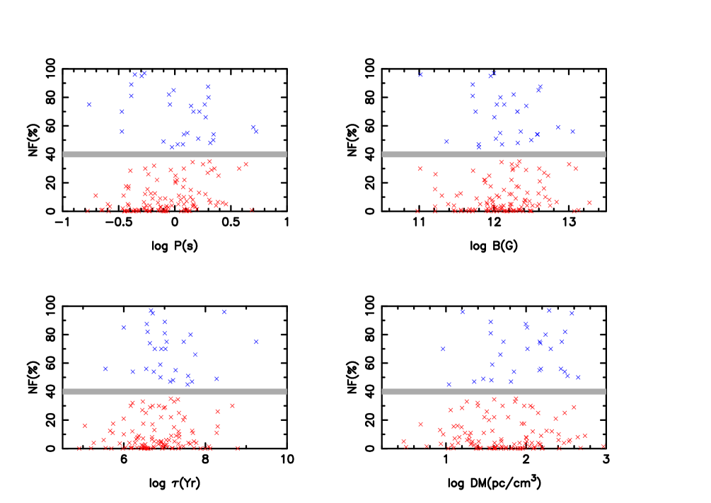
Figure 2: Variation of the nulling fraction (NF) against spin-period (P_s), surface magnetic field (B_s), characteristic age ($\tau_{\rm c}$) and dispersion measure (DM) of pulsars. The red points correspond to pulsars with low NF ($<$ 40%) and the blue points to pulsars with larger values of NF. The horizontal grey band highlights the apparent gap in NF values around 40%.

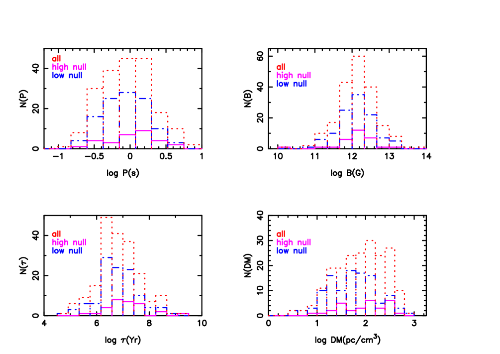
Figure 3: Distribution of characteristic pulsar parameters for pulsars with high null (NF $<$ 40%), with low null (NF $>$ 40%), and all of the nulling pulsars. It is to be noted that the histogram for all nulling pulsars also include pulsars without any estimate for NF and the intermittent pulsars.

From Fig.3, it can be seen that the earlier conjecture, that nulling is predominantly experienced by old radio pulsars with relatively smaller magnetic fields, appears to be ruled out by the current population.

Interestingly, the nature of the distribution of the intrinsic parameters appear to be very different for pulsars exhibiting high NF compared to those having low values of NF. A nominal Kolmogorov-Smirnov (KS) test [von Mises (1980)] on the spin-period of nulling pulsars with higher and lower values of NF, yields P_KS = 0.002 and D_KS = 0.322, rejecting the null hypothesis that these two populations have the same underlying distribution. [Here P_KS indicates the probability that the two distributions are inherently similar (identical), whereas D_KS is the maximum value of the absolute difference between the two distributions.] This is also evident from the fractional plot of period distributions shown in Fig.4.

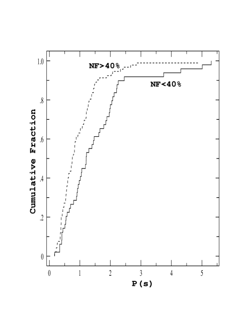
Figure 4: Cumulative fraction plot for the P_s distribution of pulsars with low ($<$ 40%) and high ($>$ 40%) values of NF.

3 Pulsar Death-Lines

Clearly, the nature of the emission mechanism must have a bearing on the nulling behaviour, whether or not nulling is directly related to the age of a pulsar. As mentioned earlier, ?) undertook the first comprehensive study of nulling pulsars and suggested that the time interval between regular bursts of pulse emission increases with age, eventually leading to pulsar ‘death’. This study explicitly defined, for the very first time, a cut-off line for pulsar emission. This can be thought of as the precursor of more formal ‘death-line’s to be developed afterwards. Later, ?) also suggested that nulling pulsars are likely to be very close to the death line, being active only when favourable conditions prevail.

Irrespective of the underlying mechanism, copious pair production in the magnetosphere is understood to be the basic requirement for pulsar emission. Such pair production gives rise to a dense plasma that can then allow the growth of a number of coherent instabilities and generate highly relativistic secondary pairs which then produce the radio band emission (see [Mitra et al. (2009)], [Melrose (2017)] and references therein for details of and recent progresses made in the area of pulsar emission physics).

Pulsars ‘switch off’ when conditions for pair production fail to be met. Depending on the specific model, radio pulsar ‘death line’ is defined to be a relation between P_s & $\dot{\rm P}$  (period derivative) or P_s & B_s beyond which the process of pair-production ceases and a pulsar stops emitting. A number of theoretical models, consequently a variety of death-lines have been proposed to explain the present crop of pulsars. All of these require some degree of anomalous field configuration (higher multipole components or an offset dipole) to interpret the data in its entirety. Some of the most representative death-lines, based upon different models of emission mechanism, are described below.

In the following equations - $B_{\rm p}$ is the dipolar field, $B_{\rm s}$ is the surface field, $r_{\rm c}$ is the radius of curvature for the magnetic field, $h$ is the thickness of the polar cap gap, $R$ is the stellar radius and $\Omega$ is the stellar spin frequency. The value of inclination angle chosen for 5b corresponds to that for Geminga.

A. ?) :

I. Polar Cap Model : Pair production ($\gamma+B\rightarrow e^{-}+e^{+}$) predominantly happens near the polar cap of the neutron star [Ruderman & Sutherland (1975)].

01. Central Dipole, with $B_{\rm s}=B_{\rm p}$, $r_{\rm c}=(Rc/\Omega)^{1/2}$ -

$$4\log B-7.5\log P=49.3,$$ (1)

01a. Dipole, off-centre by a distance $d$ -

$$4\log B-7.5\log P=49.3-2.5\log[R/(R-d)],$$ (2)

02. Very curved field lines, with $r_{\rm c}\sim R$, $B_{\rm s}=B_{\rm p}$ -

$$4\log B-6.5\log P=45.7,$$ (3)

03. Very curved field lines, with $r_{\rm c}\sim R$, $B_{\rm s}=2\times 10^{13}$ G, $h\sim(B_{\rm p}/B_{\rm s})^{1/2}R(R\Omega/c)^{1/2}$ at polar cap -

$$7\log B-13\log P=78,$$ (4)

04a, 04b. Extremely twisted field lines, with $r_{\rm c}\sim R$ -

$$4\log B-6\log P=43.8\;\mbox{or}\;31.3\,,$$ (5)

(Whichever constant produces larger B in the equation above to ensure $E_{\rm p}>2m_{e}c^{2}$.)

II. Outer Magnetospheric Model : Pair production happens in the outer magnetosphere via inverse Compton scattering, curvature radiation or synchrotron radiation etc.

05a, 05b. Aligned/Non-Aligned Dipole -

$$5\log B-12\log P=72\;\mbox{or}\;69.5\,.$$ (6)

B. ?) : In each of the pair of equations below (depicted by the sets 06a-06b, 07a-07b, 08a-08b, 09a-09b), the first one corresponds to a dipole configuration and the second one corresponds to a multipolar configuration with $B_{\rm s}\sim B_{\rm p}$ and $r_{\rm c}\sim R$. Furthermore, $r_{\rm c6}$ is $r_{\rm c}$ in units of $10^{6}$ cm.

I. Vacuum Gap Model : Pair production happens via formation of a vacuum gap close to the polar cap.

A. Curvature Radiation -

$${\bf 06a.}\log\mbox{$\dot{\rm P}$}=11/4\log P-14.62,$$ (7)

$${\bf 06b.}\log\mbox{$\dot{\rm P}$}=9/4\log P-16.58+\log r_{\rm c6},$$ (8)

B. Inverse Compton Scattering -

$${\bf 07a.}\log\mbox{$\dot{\rm P}$}=2/11\log P-13.07,$$ (9)

$${\bf 07b.}\log\mbox{$\dot{\rm P}$}=-2/11\log P-14.50+8/11\log r_{\rm c6},$$ (10)

II. Space-Charge Limited Flow Model : If charged particles can be freely pulled out of the neutron star surface, a space-charged limited flow is generated. Mechanisms similar to those above then work to generate secondary/tertiary pairs.

A. Curvature radiation -

$${\bf 08a.}\log\mbox{$\dot{\rm P}$}=5/2\log P-14.56,$$ (11)

$${\bf 08b.}\log\mbox{$\dot{\rm P}$}=2\log P-16.52+\log r_{\rm c6},$$ (12)

B. Inverse Compton Scattering -

$${\bf 09a.}\log\mbox{$\dot{\rm P}$}=-3/11\log P-15.36,$$ (13)

$${\bf 09b.}\log\mbox{$\dot{\rm P}$}=-7/11\log P-16.79+8/11\log r_{\rm c6}.$$ (14)

All the death-lines discussed above have been indicated in the top panel of Fig.[5], in the backdrop of the known radio pulsars in P_s-B_s plane. It should be noted that while the death lines are defined in terms of the magnetic field by ?), they are defined using the derivative of spin-period ($\dot{\rm P}$) by ?). However, the magnetic field is not a measured quantity. An estimate, only for the dipolar component, is obtained from the measured quantities P_s and $\dot{\rm P}$ through the following relation [Manchester & Taylor (1977)] -

$$B_{\rm p}\simeq 3.2\times 10^{19}\left(\frac{P_{s}}{s}\right)^{\frac{1}{2}}\left(\frac{\mbox{$\dot{\rm P}$}}{ss^{-1}}\right)^{\frac{1}{2}}\leavevmode\nobreak\ \mbox{G}\,.$$ (15)

In Fig.[5], this measure of the magnetic field is used for known pulsars. The death-line equations, given in terms of P_s and $\dot{\rm P}$  by ?), are also plotted in the P_s-B_s plane using the same measure. Therefore, any conclusion drawn for this set of death-line equations do not suffer from an ambiguity regarding the measure of the magnetic field (between the dipolar and the true surface field). However, that is not correct in case of the death-lines defined by ?), which suffer from this ambiguity. It is clear that the death-lines 7a-7b, 9a-9b are not very useful in constraining the radio pulsar population. In particular, they completely fail to accommodate the millisecond pulsars. Even if one questions whether the same death-line works for both the ordinary and millisecond pulsars, because these equations also preclude a significant number of relatively low field pulsars, we shall not consider them hereafter. On the other hand, the death-line depicted by 4b is far too deep into the ‘graveyard’ to be of much use for the current population of pulsars. Perhaps the newly discovered long-period pulsars (some of which have been indicated by red stars in the bottom panel of Fig.[5]) are likely to be constrained by this equation. Among the rest, 1, 6a and 2, 6b are pairwise coincident (almost); while 2, 3 and 4 envelope somewhat similar regions. (8a, 8b are, more or less, coincident with 6a, 6b and therefore not shown in the figure.)

In the bottom panel of Fig.[5] the nulling pulsars (along with intermediate pulsars) are shown along with a relevant subset of death-lines. A number of (non-nulling) pulsars have been also been identified for their importance in the context of death-lines. For example, despite the wide variety of models and the large number of possible death-lines described above, it was necessary to invoke higher multipoles, many orders of magnitude stronger than the dipole, at the the surface to accommodate the 8.5 s pulsar J2144-3933 ?). Other pulsars, like J1232-3933 [Jacoby et al. (2009)], J1333-4449 [Jacoby et al. (2009)] or J2123+5454 [Stovall et al. (2014)] may also have similar explanations for them to work beyond the death-line 4a. It is to be noted that J0250+5854 [Tan et al. (2018)], the famous slow pulsar (P_s = 23.5s), is actually within the allowed-zone, as far as death-lines are concerned.

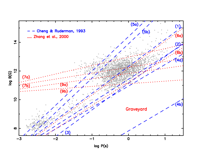
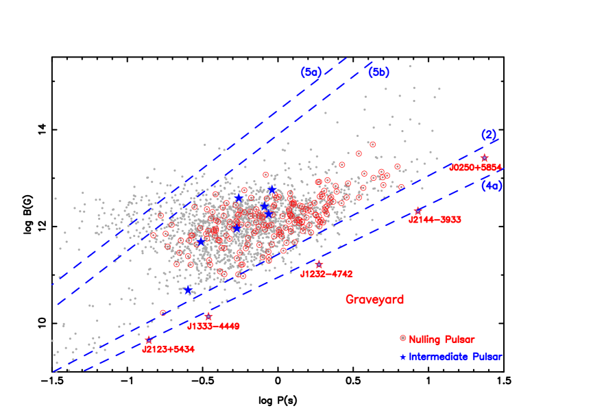
Figure 5: Observed radio pulsars and theoretical death-lines in the P_s-B_s plane. Top Panel - The death lines have been marked according to their numbering in the text. Bottom Panel - Nulling pulsars and intermediate pulsars have been highlighted with a small subset of death-lines. A number of pulsars have been specially identified (red open star) which appear to be functioning beyond the least stringent death line. The data for the known pulsars have been obtained from the ATNF pulsar catalog - http://www.atnf.csiro.au/research/pulsar/psrcat/ (Manchester et al., 2005).

It is likely that more than one emission mechanism could be responsible for radio pulsars activity [Chen & Ruderman (1993)]. It is then plausible that different death-lines are appropriate for pulsars in which different mechanisms are responsible for the emission. Though, at present, there is no clear understanding of this. However, when the population of nulling pulsars are marked out in the P_s-B_s plane, certain remarkable things are noticed. It can be seen from the bottom panel of Fig.[5] that there are almost no nulling pulsar above the death-line 5b (definitely none above 5a). Now, 5a, 5b correspond to pure dipolar field configurations (aligned or non-aligned with the rotation axis) in an outer magnetospheric model. Given the current understanding of pulsar emission process, this may mean that the nulling pulsars likely do not possess purely dipolar field configurations where emission originates in the outer magnetosphere. On the other hand, the nulling pulsars appear to be bounded below by death-line 2, which corresponds to a polar cap emission model with very curved field lines (curvature radius $\sim$ stellar radius). Taken together, it is suggestive of the conclusion that the pulsars for which the emission is predominantly from the polar cap and the magnetic field is extremely curved are likely to experience nulling episodes.

It has been suggested that in some pulsars, the magnetosphere may occasionally switch (‘mode change’) between different states with different geometries or/and different distributions of currents [Timokhin (2010)]. These states have different spin-down rates and emission beams; and some of the states do not (or apparently not) have any radio emission. In case of the intermittent pulsar, B1931+24, it has been clearly seen that $\dot{\rm P}$ significantly differs from the off-state (nulling phase) to the on-state (active phase). It has been argued that, in the off-phase, the open field lines above the magnetic pole become depleted of charged particles and the rotational slow down happens purely due to the magnetic dipole radiation. On the other hand, in the on-phase, an additional slow-down torque is provided by the out-flowing plasma [Kramer et al. (2006a)]. Therefore, an estimate of the dipolar magnetic field obtained from measurements made during the active phase is always an overestimate. On the other hand, ?) has reported to have observed no change in the spin-down rate for the pulsar B0823+26 between the off-state and the on-state. This implies that there would be no overestimate of the dipolar field for this pulsar. Given this, it is difficult to gauge whether the reported values of $\dot{\rm P}$ and hence that of the dipolar field is an overestimate or not. However, even with a 10% overestimate (assumed for all the nulling pulsars), we find that our conclusions drawn above remain unchanged.

It is clear from the bottom-panel of Fig.[5] that quite a large number of pulsars are active beyond the death-line 2, but are bounded by the death-line 4a which again corresponds to polar-cap emission but the magnetic field configurations for this case are extremely twisted. Because the pulsars in this region (between death-lines 2 and 4a) are slow objects with no apparent significance they have mostly not been studied in detail. To our knowledge, there does not exist any study that specifically investigates the nulling behaviour of pulsars in this region. However, it is quite clear that if these objects are carefully monitored, for the presence of any nulling episodes, we would be able to gauge the validity of the conclusion above. With this in mind, we are initiating such a program, of targeted observation of slow pulsars between the death-lines 2 and 4a, with the Giant Meterwave Radio Telescope [Konar et al. (2019)].

4 Summary

About 8% of all known radio pulsars have been observed to exhibit nulling. In this work, we have considered NF to be the marker (for want of any other characteristic parameter which has been estimated for a significant number of nulling pulsars) for a pulsar’s nulling behaviour and have looked at the nature of its distribution. We have also considered the general characteristics (in terms of intrinsic pulsar parameters) of this sub-population of radio pulsars. The conclusions drawn are summarised as follows -

1. There appears to be a gap in the estimated value of nulling fraction around 40%, separating pulsars into two populations exhibiting higher and lower values of NF. However, this should be taken with a bit of caution, as inaccurate estimates of NF and inadequate study of pulsars with NF near 40% could contribute to this bias. On the other hand, the error bars, even though these could be quite large on occasion (tables [2 - 5]), do not appear likely to smudge out the gap.

2. The number of pulsars with a lower value ($<$40%) of NF appear to be far more in comparison to the ones with a higher value of NF (Fig.[1]). Once again, this could simply be an artifact of observational bias. For example, pulsars with very high NF are quite likely to be entirely missed by rapid pulsar surveys where other pulsars with zero (or small) nulling fractions are detected easily.

3. The distributions of the intrinsic pulsar parameters (P_s, $\dot{\rm P}$, B_s, $\tau_{\rm c}$, DM etc.) are statistically different in these two populations of pulsars with high and low values of NF.

4. There is no evidence of any correlation of NF with any of the intrinsic pulsar parameters as per present data. This behaviour is similar for pulsars with high as well as low values of NF.

5. The most interesting conclusion of our study is regarding the nature of the nulling pulsars. It appears likely that pulsars, for which the emission is predominantly from the polar cap and have extremely curved magnetic fields, preferentially experience nulling episodes. If borne out by future observations, this would pave the way for a theory of nulling which has so far eluded us.

6. Regular and targeted monitoring of pulsars in the region close to and bounded by the death-lines 2 and 4a is therefore of great importance. As mentioned earlier, we are initiating a study with this goal.

5 Acknowledgment

Most of this work had been carried out when SK was supported by a grant (SR/WOS-A/PM-1038/2014) from DST, Government of India and UD was supported through the ‘Indian Academies’ Summer Research Fellowship Programme (2017)’. Work done by Devansh Agarwal (also as a part of another summer project) has been useful in sorting out certain preliminary issues. SK would also like to thank Avinash Deshpande, Yashwant Gupta, Vishal Gajjar and Bhal Chandra Joshi for helpful discussions. We also thank the anonymous referee for helping to improve the clarity of the manuscript significantly.

Appendix A Nulling Pulsar Parameters

Table 2: Characteristic parameters - spin-period (P_s), surface magnetic field (B_s) and nulling fraction (NF) of known nulling pulsars. The P_s and B_s values are taken from the ATNF database (http://www.atnf.csiro.au/research/pulsar/psrcat/) while NF values have been indicated with appropriate references, inclusive of cases where different estimates have been reported by different groups.

	PR’S Name	J-Name	Ps	Bs	NF	References
			(s)	(G)	(%)
1	B0031-07	J0034-0721	0.9429	$6.28\times 10^{11}$	$44.0\pm 1.0$	[Gajjar (2017)]
2	B0045+33	J0048+3412	1.2171	$1.71\times 10^{12}$	$21.0\pm 1.0$	[Redman & Rankin (2009)]
3	B0148-06	J0151-0635	1.4647	$8.15\times 10^{11}$	$\leq 5.0$	[Biggs (1992)]
4	B0149-16	J0152-1637	0.8327	$1.05\times 10^{12}$	$\leq 2.5$	[Vivekanand (1995)]
5	B0301+19	J0304+1932	1.3876	$1.36\times 10^{12}$	$10.0$	[Rankin (1986)]
6	B0329+54	J0332+5434	0.7145	$1.22\times 10^{12}$	$\leq 0.25$	[Ritchings (1976)]
7	B0450-18	J0452-1759	0.5489	$1.80\times 10^{12}$	$\leq 0.5$	[Ritchings (1976)]
8	J0458-0505	J0458-0505	1.8835	$1.01\times 10^{12}$	$63.0\pm 3.0$	[Lynch et al. (2013)]
9	B0523+11	J0525+1115	0.3544	$1.63\times 10^{11}$	$\leq 0.06$	[Weisberg et al. (1986)]
10	B0525+21	J0528+2200	3.7455	$1.24\times 10^{13}$	$25.0\pm 5.0$	[Ritchings (1976)]
11	B0529-66	J0529-6652	0.9757	$3.94\times 10^{12}$	$83.5\pm 1.5$	[Crawford et al. (2013)]
12	B0626+24	J0629+2415	0.4766	$9.87\times 10^{11}$	$\leq 0.02$	[Weisberg et al. (1986)]
13	B0628-28	J0630-2834	1.2444	$3.01\times 10^{12}$	$\leq 0.3$	[Biggs (1992)]
14	B0656+14	J0659+1414	0.3849	$4.66\times 10^{12}$	$12.0\pm 4.0$	[Weisberg et al. (1986)]
15	B0736-40	J0738-4042	0.3749	$7.88\times 10^{11}$	$\leq 0.4$	[Biggs (1992)]
16	B0740-28	J0742-2822	0.1668	$1.69\times 10^{12}$	$\leq 0.2$	[Biggs (1992)]
17	B0751+32	J0754+3231	1.4423	$1.26\times 10^{12}$	$34.0\pm 0.5$	[Weisberg et al. (1986)]
18	B0809+74	J0814+7429	1.2922	$4.72\times 10^{11}$	$\leq 5.0$	[Ritchings (1976)]
19	B0818-13	J0820-1350	1.2381	$1.63\times 10^{12}$	$1.5\pm 0.25$	[Ritchings (1976)]
20	B0818-41	J0820-4114	0.5454	$1.03\times 10^{11}$	$30.0$	[Bhattacharyya et al. (2010)]
21	B0820+02	J0823+0159	0.8649	$3.04\times 10^{11}$	$\leq 0.06$	[Weisberg et al. (1986)]
22	B0823+26	J0826+2637	0.5307	$9.64\times 10^{11}$	$6.4\pm 0.8$	[Rankin & Rathnasree (1995)]
23	B0826-34	J0828-3417	1.8489	$1.37\times 10^{12}$	$75.0\pm 35.0$	[Durdin et al. (1979)]
24	B0833-45	J0835-4510	0.0893	$3.38\times 10^{12}$	$\leq 0.0008$	[Biggs (1992)]
25	B0834+06	J0837+0610	1.2738	$2.98\times 10^{12}$	$7.1\pm 0.1$	[Ritchings (1976)]
26	B0835-41	J0837-4135	0.7516	$1.65\times 10^{12}$	$1.7\pm 1.2$	[Gajjar (2017)]
27	B0906-17	J0908-1739	0.4016	$5.25\times 10^{11}$	$26.8\pm 1.7$	[Basu et al. (2017)]
				$5.25\times 10^{11}$	$25.7\pm 1.3$	[Basu et al. (2017)]
28	B0919+06	J0922+0638	0.4306	$2.46\times 10^{12}$	$\leq 0.05$	[Weisberg et al. (1986)]
29	B0932-52	J0934-5249	1.4448	$2.62\times 10^{12}$	$5.0\pm 3.0$	[Naidu et al. (2017)]
30	B0940-55	J0942-5552	0.6644	$3.94\times 10^{12}$	$\leq 12.5$	[Biggs (1992)]
31	B0940+16	J0943+1631	1.0874	$3.18\times 10^{11}$	$8.0\pm 3.0$	[Weisberg et al. (1986)]
32	B0942-13	J0944-1354	0.5703	$1.63\times 10^{11}$	$14.4\pm 0.9$	[Basu et al. (2017)]
					$\leq 7.0$	[Vivekanand (1995)]
33	B0950+08	J0953+0755	0.2531	$2.44\times 10^{11}$	$\leq 5.0$	[Ritchings (1976)]
34	J1049-5833	J1049-5833	2.2023	$3.15\times 10^{12}$	$47.0\pm 3.0$	[Wang et al. (2007)]
					$47.0\pm 3.0$	[Yang et al. (2014)]
35	B1055-52	J1057-5226	0.1971	$1.09\times 10^{12}$	$\leq 11.0$	[Biggs (1992)]
36	B1112+50	J1115+5030	1.6564	$2.06\times 10^{12}$	$64.0\pm 6.0$	[Gajjar (2017)]
37	B1114-41	J1116-4122	0.9432	$2.77\times 10^{12}$	$3.3\pm 0.5$	[Basu et al. (2017)]
38	B1133+16	J1136+1551	1.1879	$2.13\times 10^{12}$	$15.0\pm 2.5$	[Ritchings (1976)]
39	B1237+25	J1239+2453	1.3824	$1.17\times 10^{12}$	$6.0\pm 2.5$	[Ritchings (1976)]
					$7.0\pm 3.0$	[Naidu et al. (2017)]
40	B1240-64	J1243-6423	0.3885	$1.34\times 10^{12}$	$\leq 4.0$	[Biggs (1992)]

Table 3: Continuation of Table 2.

	PSR Name	J-Name	Ps	Bs	NF	References
			(s)	(G)	(%)
41	B1322-66	J1326-6700	0.5430	$1.72\times 10^{12}$	$9.1\pm 3.0$	[Wang et al. (2007)]
42	B1325-49	J1328-4921	1.4787	$9.61\times 10^{11}$	$4.0$	[Basu et al. (2017)]
43	B1358-63	J1401-6357	0.8428	$3.80\times 10^{12}$	$1.6\pm 2.0$	[Wang et al. (2007)]
44	B1426-66	J1430-6623	0.7854	$1.49\times 10^{12}$	$\leq 0.05$	[Biggs (1992)]
45	B1451-68	J1456-6843	0.2634	$1.63\times 10^{11}$	$\leq 3.3$	[Biggs (1992)]
46	J1502-5653	J1502-5653	0.5355	$9.99\times 10^{11}$	$93.0\pm 4.0$	[Wang et al. (2007)]
47	B1508+55	J1509+5531	0.7397	$1.95\times 10^{12}$	$7.0\pm 2.0$	[Naidu et al. (2017)]
48	J1525-5417	J1525-5417	1.0117	$4.09\times 10^{12}$	$16.0\pm 5.0$	[Wang et al. (2007)]
49	B1524-39	J1527-3931	2.4176	$6.87\times 10^{12}$	$5.1\pm 1.3$	[Basu et al. (2017)]
50	B1530+27	J1532+2745	1.1248	$9.48\times 10^{11}$	$6.0\pm 2.0$	[Weisberg et al. (1986)]
51	B1530-53	J1534-5334	1.3689	$1.41\times 10^{12}$	$\leq 0.25$	[Biggs (1992)]
52	B1540-06	J1543-0620	0.7091	$7.99\times 10^{11}$	$4.0\pm 2.0$	[Naidu et al. (2017)]
53	B1556-44	J1559-4438	0.2571	$5.18\times 10^{11}$	$\leq 0.01$	[Biggs (1992)]
					$0.24$	[Basu et al. (2017)]
54	B1604-00	J1607-0032	0.4218	$3.64\times 10^{11}$	$\leq 0.1$	[Biggs (1992)]
55	B1612+07	J1614+0737	1.2068	$1.71\times 10^{12}$	$\leq 5.0$	[Weisberg et al. (1986)]
56	J1634-5107	J1634-5107	0.5074	$9.04\times 10^{11}$	$90.0\pm 5.0$	[Young et al. (2015)]
57	J1639-4359	J1639-4359	0.5876	$9.50\times 10^{10}$	$\leq 0.1$	[Gajjar (2017)]
58	B1641-45	J1644-4559	0.4551	$3.06\times 10^{12}$	$\leq 0.4$	[Biggs (1992)]
59	B1642-03	J1645-0317	0.3877	$8.41\times 10^{11}$	$\leq 0.25$	[Ritchings (1976)]
60	J1648-4458	J1648-4458	0.6296	$1.09\times 10^{12}$	$1.4$	[Wang et al. (2007)]
61	J1649+2533	J1649+2533	1.0153	$7.63\times 10^{11}$	$\leq 20.0$	[Redman & Rankin (2009)]
62	B1658-37	J1701-3726	2.4546	$5.29\times 10^{12}$	$14.0\pm 2.0$	[Yang et al. (2014)]
					$19.0\pm 6.0$	[Gajjar (2017)]
63	J1702-4428	J1702-4428	2.1235	$2.68\times 10^{12}$	$26.0\pm 3.0$	[Wang et al. (2007)]
64	B1700-32	J1703-3241	1.2118	$9.05\times 10^{11}$	$1.6\pm 0.4$	[Basu et al. (2017)]
65	J1703-4851	J1703-4851	1.3964	$2.70\times 10^{12}$	$1.1$	[Wang et al. (2007)]
					$74.0$	[Yang et al. (2014)]
66	B1706-16	J1709-1640	0.6531	$2.05\times 10^{12}$	$31.0\pm 2.0$, $15.0$	[Naidu et al. (2018)]
67	J1715-4034	J1715-4034	2.0722	$2.53\times 10^{12}$	$\leq 6.0$	[Gajjar (2017)]
68	B1713-40	J1717-4054	0.8877	$1.83\times 10^{12}$	$77.0\pm 5.0$	[Young et al. (2015)]
					$\geq 95.0$	[Wang et al. (2007)]
69	B1718-32	J1722-3207	0.4772	$5.62\times 10^{11}$	$1.0\pm 1.0$	[Naidu et al. (2017)]
70	J1725-4043	J1725-4043	1.4651	$2.05\times 10^{12}$	$\leq 70.0$	[Gajjar (2017)]
71	J1727-2739	J1727-2739	1.2931	$1.21\times 10^{12}$	$52.0\pm 3.0$	[Wang et al. (2007)]
72	B1727-47	J1731-4744	0.8298	$1.18\times 10^{13}$	$\leq 0.1$	[Biggs (1992)]
73	B1730-37	J1733-3716	0.3376	$2.28\times 10^{12}$	$52.4\pm 3.5$	[Basu et al. (2017)]
74	J1738-2330	J1738-2330	1.9788	$4.16\times 10^{12}$	$85.1\pm 2.3$	[Gajjar (2017)]
75	B1737+13	J1740+1311	0.8031	$1.09\times 10^{12}$	$\leq 0.02$	[Weisberg et al. (1986)]
76	B1738-08	J1741-0840	2.0431	$2.18\times 10^{12}$	$30.0\pm 5.0$	[Gajjar et al. (2017)]
					$15.7\pm 1.7$, $15.8\pm 1.4$	[Basu et al. (2017)]
77	J1744-3922	J1744-3922	0.1724	$1.65\times 10^{10}$	$\leq 75.0$	[Faulkner et al. (2004)]
78	B1742-30	J1745-3040	0.3674	$1.99\times 10^{12}$	$\leq 17.5$	[Biggs (1992)]
79	B1747-46	J1751-4657	0.7424	$9.91\times 10^{11}$	$2.4\pm 0.5$	[Basu et al. (2017)]
80	J1752+2359	J1752+2359	0.4091	$5.19\times 10^{11}$	$\leq 89.0$	[Gajjar (2017)]
81	B1749-28	J1752-2806	0.5626	$2.16\times 10^{12}$	$\leq 0.75$	[Ritchings (1976)]
82	J1752+2359	J1752+2359	0.4091	$5.19\times 10^{11}$	$81.0$	[Yang et al. (2014)]
83	B1758-03	J1801-0357	0.9215	$1.77\times 10^{12}$	$27.7\pm 1.3$, $26.1\pm 2.6$	[Basu et al. (2017)]
84	J1808-0813	J1808-0813	0.8760	$1.05\times 10^{12}$	$1.28\pm 1.3$	[Basu et al. (2017)]
85	B1809-173	J1812-1718	1.2054	$4.85\times 10^{12}$	$5.8\pm 0.4$	[Wang et al. (2007)]

Table 4: Continuation of Table 2 & 3.

	PSR Name	J-Name	Ps	Bs	NF	References
			(s)	(G)	(%)
86	B1813-36	J1817-3618	0.3870	$9.01\times 10^{11}$	$16.7\pm 0.7$	[Basu et al. (2017)]
87	J1819+1305	J1819+1305	1.0604	$6.25\times 10^{11}$	$41.0\pm 6.0$	[Yang et al. (2014)]
88	B1818-04	J1820-0427	0.5981	$1.97\times 10^{12}$	$\leq 0.25$	[Biggs (1992)]
89	J1820-0509	J1820-0509	0.3373	$5.67\times 10^{11}$	$67.0\pm 3.0$	[Wang et al. (2007)]
90	B1819-22	J1822-2256	1.8743	$1.61\times 10^{12}$	$10.0\pm 2.0$	[Naidu et al. (2017)]
					$4.7\pm 0.9$	[Basu et al. (2017)]
					$5.5\pm 0.7$	–do–
91	B1821+05	J1823+0550	0.7529	$4.18\times 10^{11}$	$\leq 0.4$	[Weisberg et al. (1986)]
92	J1831-1223	J1831-1223	2.8580	$3.99\times 10^{12}$	$4.0\pm 1.0$	[Wang et al. (2007)]
93	J1833-1055	J1833-1055	0.6336	$5.85\times 10^{11}$	$7.0\pm 2.0$	[Wang et al. (2007)]
94	J1840-0840	J1840-0840	5.3094	$1.13\times 10^{13}$	$50.0\pm 6.0$	[Gajjar et al. (2017)]
95	B1839+09	J1841+0912	0.3813	$6.52\times 10^{11}$	$\leq 5.0$	[Weisberg et al. (1986)]
96	J1843-0211	J1843-0211	2.0275	$5.48\times 10^{12}$	$6.0\pm 2.0$	[Wang et al. (2007)]
97	B1842+14	J1844+1454	0.3755	$8.48\times 10^{11}$	$\leq 0.15$	[Weisberg et al. (1986)]
98	B1844-04	J1847-0402	0.5978	$5.63\times 10^{12}$	$3.0\pm 1.0$	[Naidu et al. (2017)]
99	B1845-19	J1848-1952	4.3082	$1.01\times 10^{13}$	$27.0\pm 6.0$	[Naidu et al. (2017)]
100	B1848+12	J1851+1259	1.2053	$3.77\times 10^{12}$	$\leq 54.0$	[Redman & Rankin (2009)]
101	J1853+0505	J1853+0505	0.9051	$1.09\times 10^{12}$	$67.0\pm 8.0$	[Young et al. (2015)]
102	B1857-26	J1900-2600	0.6122	$3.58\times 10^{11}$	$10.0\pm 2.5$	[Ritchings (1976)]
103	J1901+0413	J1901+0413	2.6631	$1.89\times 10^{13}$	$\leq 6.0$	[Gajjar (2017)]
104	J1901-0906	J1901-0906	1.7819	$1.73\times 10^{12}$	$29.0\pm 4.0$	[Naidu et al. (2017)]
					$2.9$	[Basu et al. (2017)]
					$5.6\pm 0.7$	–do–
105	B1907+03	J1910+0358	2.3303	$3.27\times 10^{12}$	$4.0\pm 0.2$	[Weisberg et al. (1986)]
106	B1911-04	J1913-0440	0.8259	$1.85\times 10^{12}$	$\leq 0.5$	[Ritchings (1976)]
107	J1916+1023	J1916+1023	1.6183	$1.06\times 10^{12}$	$47.0\pm 4.0$	[Wang et al. (2007)]
108	B1917+00	J1919+0021	1.2723	$3.16\times 10^{12}$	$\leq 0.4$	[Rankin (1986)]
109	J1920+1040	J1920+1040	2.2158	$3.83\times 10^{12}$	$50.0\pm 4.0$	[Wang et al. (2007)]
110	B1918+19	J1921+1948	0.8210	$8.68\times 10^{11}$	$9.0$, $43.0$	[Rankin et al. (2013)]
111	B1919+21	J1921+2153	1.3373	$1.36\times 10^{12}$	$\leq 0.25$	[Ritchings (1976)]
112	J1926-1314	J1926-1314	4.8643	$1.35\times 10^{13}$	$\sim 75.7\pm 1.9$	[Rosen et al. (2013)]
113	B1923+04	J1926+0431	1.0741	$1.64\times 10^{12}$	$\leq 5.0$	[Weisberg et al. (1986)]
114	B1929+10	J1932+1059	0.2265	$5.18\times 10^{11}$	$\leq 1.0$	[Ritchings (1976)]
115	B1933+16	J1935+1616	0.3587	$1.48\times 10^{12}$	$\leq 0.06$	[Biggs (1992)]
116	B1942+17	J1944+1755	1.9969	$1.22\times 10^{12}$	$\leq 60.0$	[Lorimer et al. (2002)]
117	B1942-00	J1945-0040	1.0456	$7.57\times 10^{11}$	$21.0\pm 1.0$	[Weisberg et al. (1986)]
118	B1944+17	J1946+1805	0.4406	$1.04\times 10^{11}$	$55.0\pm 5.0$	[Yang et al. (2014)]
					$64.0\pm 32.0$	[Ritchings (1976)]
119	B1946+35	J1948+3540	0.7173	$2.28\times 10^{12}$	$\leq 0.75$	[Ritchings (1976)]
120	B2003-08	J2006-0807	0.5809	$1.65\times 10^{11}$	$15.5\pm 1.0$	[Basu et al. (2017)]
121	B2016+28	J2018+2839	0.5580	$2.91\times 10^{11}$	$1.0\pm 3.0$	[Naidu et al. (2017)]
122	B2020+28	J2022+2854	0.3434	$8.16\times 10^{11}$	$0.2\pm 1.6$	[Gajjar (2017)]
123	B2021+51	J2022+5154	0.5292	$1.29\times 10^{12}$	$1.4\pm 0.7$	[Gajjar (2017)]
124	J2033+0042	J2033+0042	5.0134	$7.21\times 10^{12}$	$44-49,53-58$	[Lynch et al. (2013)]
125	B2034+19	J2037+1942	2.0744	$2.08\times 10^{12}$	$44.0\pm 4.0$	[Herfindal & Rankin (2009)]
					$24.2\pm 1.5$	–do–

Table 5: Continuation of Table 2, 3 & 4.

	PSR Name	J-Name	Ps	Bs	NF	References
			(s)	(G)	(%)
126	B2044+15	J2046+1540	1.1383	$4.61\times 10^{11}$	$\leq 0.04$	[Weisberg et al. (1986)]
127	B2045-16	J2048-1616	1.9616	$4.69\times 10^{12}$	$22.0\pm 5.0$	[Naidu et al. (2017)]
					$5.5\pm 0.2$	[Basu & Mitra (2018)]
128	B2053+36	J2055+3630	0.2215	$2.89\times 10^{11}$	$\leq 0.7$	[Weisberg et al. (1986)]
129	B2110+27	J2113+2754	1.2028	$1.78\times 10^{12}$	$\leq 30.0$	[Redman & Rankin (2009)]
130	B2111+46	J2113+4644	1.0147	$8.62\times 10^{11}$	$21.0\pm 4.0$	[Gajjar (2017)]
131	B2113+14	J2116+1414	0.4402	$3.61\times 10^{11}$	$\leq 1.0$	[Weisberg et al. (1986)]
132	B2122+13	J2124+1407	0.6941	$7.39\times 10^{11}$	$\leq 22.0$	[Redman & Rankin (2009)]
133	B2154+40	J2157+4017	1.5253	$2.32\times 10^{12}$	$7.5\pm 2.5$	[Ritchings (1976)]
134	J2208+5500	J2208+5500	0.9332	$2.58\times 10^{12}$	$\leq 7.5$	[Joshi et al. (2009)]
135	B2217+47	J2219+4754	0.5385	$1.23\times 10^{12}$	$\leq 2.0$	[Ritchings (1976)]
136	J2253+1516	J2253+1516	0.7922	$2.32\times 10^{11}$	$\leq 49.0$	[Redman & Rankin (2009)]
137	B2303+30	J2305+3100	1.5759	$2.16\times 10^{12}$	$1.0$	[Rankin (1986)]
138	B2310+42	J2313+4253	0.3494	$2.01\times 10^{11}$	$\leq 11.0$	[Redman & Rankin (2009)]
139	B2315+21	J2317+2149	1.4447	$1.24\times 10^{12}$	$3.0\pm 0.5$	[Weisberg et al. (1986)]
140	B2319+60	J2321+6024	2.2565	$4.03\times 10^{12}$	$29.0\pm 1.0$	[Gajjar (2017)]
141	B2327-20	J2330-2005	1.6436	$2.79\times 10^{12}$	$12.0\pm 1.0$	[Biggs (1992)]
142	J2346-0609	J2346-0609	1.1815	$1.28\times 10^{12}$	$42.5\pm 3.8$	[Basu et al. (2017)]
					$28.7\pm 1.8$	[Basu et al. (2017)]

Table 6: P_s and B_s of known nulling pulsars for which no NF estimates are available.

	PSR Name	J-Name	Ps	Bs	References
			(s)	(G)
1	J0229+20	J0229+20	0.8069	NA	[Deneva et al. (2013)]
2	J0726-2612	J0726-2612	3.4423	$3.21\times 10^{13}$	[Burke-Spolaor et al. (2012)]
3	B0853-33	J0855-3331	1.2675	$2.86\times 10^{12}$	[Burke-Spolaor et al. (2012)]
4	J0941-39	J0941-39	0.5868	NA	[Burke-Spolaor & Bailes (2010)]
5	J0943+2253	J0943+2253	0.5330	$2.21\times 10^{11}$	[Brinkman et al. (2018)]
6	J1012-5830	J1012-5830	2.1336	$9.07\times 10^{12}$	[Burke-Spolaor et al. (2012)]
7	J1055-6905	J1055-6905	2.9193	$7.80\times 10^{12}$	[Burke-Spolaor et al. (2012)]
8	B1056-57	J1059-5742	1.1850	$2.28\times 10^{12}$	[Burke-Spolaor et al. (2012)]
9	J1129-53	J1129-53	1.0629	NA	[Burke-Spolaor et al. (2012)]
10	B1131-62	J1133-6250	1.0229	$6.88\times 10^{11}$	[Burke-Spolaor et al. (2012)]
11	B1154-62	J1157-6224	0.4005	$1.27\times 10^{12}$	[Burke-Spolaor et al. (2012)]
12	J1225-6035	J1225-6035	0.6263	$4.30\times 10^{11}$	[Burke-Spolaor et al. (2012)]
13	J1255-6131	J1255-6131	0.6580	$1.64\times 10^{12}$	[Burke-Spolaor et al. (2012)]
14	J1307-6318	J1307-6318	4.9624	$1.04\times 10^{13}$	[Burke-Spolaor et al. (2012)]
15	B1323-58	J1326-5859	0.4780	$1.26\times 10^{12}$	[Burke-Spolaor et al. (2012)]
16	B1323-63	J1326-6408	0.7927	$1.59\times 10^{12}$	[Burke-Spolaor et al. (2012)]
17	J1406-5806	J1406-5806	0.2883	$4.25\times 10^{11}$	[Burke-Spolaor et al. (2012)]
18	J1423-6953	J1423-6953	0.3334	$7.04\times 10^{11}$	[Burke-Spolaor et al. (2012)]
19	B1424-55	J1428-5530	0.5703	$1.10\times 10^{12}$	[Burke-Spolaor et al. (2012)]
20	B1449-64	J1453-6413	0.1795	$7.10\times 10^{11}$	[Burke-Spolaor et al. (2012)]
21	B1454-51	J1457-5122	1.7483	$3.08\times 10^{12}$	[Burke-Spolaor et al. (2012)]
22	B1510-48	J1514-4834	0.4548	$6.56\times 10^{11}$	[Burke-Spolaor et al. (2012)]
23	J1514-5925	J1514-5925	0.1488	$6.63\times 10^{11}$	[Burke-Spolaor et al. (2012)]
24	B1555-55	J1559-5545	0.9572	$4.48\times 10^{12}$	[Burke-Spolaor et al. (2012)]
25	J1624-4613	J1624-4613	0.8712	$2.33\times 10^{11}$	[Burke-Spolaor et al. (2012)]
26	B1630-44	J1633-4453	0.4365	$1.67\times 10^{12}$	[Burke-Spolaor et al. (2012)]
27	B1641-68	J1646-6831	1.7856	$1.76\times 10^{12}$	[Burke-Spolaor et al. (2012)]
28	J1647-3607	J1647-3607	0.2123	$1.67\times 10^{11}$	[Burke-Spolaor et al. (2012)]
29	J1649-4349	J1649-4349	0.8707	$1.98\times 10^{11}$	[Burke-Spolaor et al. (2012)]
30	B1650-38	J1653-3838	0.3050	$9.33\times 10^{11}$	[Burke-Spolaor et al. (2012)]
31	J1707-4729	J1707-4729	0.2665	$6.53\times 10^{11}$	[Burke-Spolaor et al. (2012)]
32	J1736-2457	J1736-2457	2.6422	$3.05\times 10^{12}$	[Burke-Spolaor et al. (2012)]
33	J1741-3016	J1741-3016	1.8938	$4.18\times 10^{12}$	[Burke-Spolaor et al. (2012)]
34	J1742-4616	J1742-4616	0.4124	$1.19\times 10^{11}$	[Burke-Spolaor et al. (2012)]
35	J1749+16	J1749+16	2.3117	NA	[Deneva et al. (2016)]
36	J1750+07	J1750+07	1.9088	NA	[Deneva et al. (2016)]
37	B1747-31	J1750-3157	0.9104	$4.28\times 10^{11}$	[Burke-Spolaor et al. (2012)]
38	J1757-2223	J1757-2223	0.1853	$3.85\times 10^{11}$	[Burke-Spolaor et al. (2012)]
39	J1758-2540	J1758-2540	2.1073	$1.83\times 10^{12}$	[Burke-Spolaor et al. (2012)]
40	B1806-21	J1809-2109	0.7024	$1.66\times 10^{12}$	[Burke-Spolaor et al. (2012)]
41	J1819-1458	J1819-1458	4.2632	$5.01\times 10^{13}$	[Burke-Spolaor et al. (2012)]
42	J1823-1126	J1823-1126	1.8465	$8.31\times 10^{12}$	[Burke-Spolaor et al. (2012)]
43	B1822-14	J1825-1446	0.2792	$2.55\times 10^{12}$	[Burke-Spolaor et al. (2012)]
44	J1827-0750	J1827-0750	0.2705	$6.54\times 10^{11}$	[Burke-Spolaor et al. (2012)]
45	J1830-1135	J1830-1135	6.2216	$1.74\times 10^{13}$	[Burke-Spolaor et al. (2012)]

Table 7: Continuation of Table 6.

	PSR Name	J-Name	Ps	Bs	References
			(s)	(G)
46	B1834-06	J1837-0653	1.9058	$1.23\times 10^{12}$	[Burke-Spolaor et al. (2012)]
47	J1837-1243	J1837-1243	1.8760	$8.38\times 10^{12}$	[Burke-Spolaor et al. (2012)]
48	J1840-1419	J1840-1419	6.5976	$6.54\times 10^{12}$	[Burke-Spolaor et al. (2012)]
49	J1841-0310	J1841-0310	1.6577	$7.54\times 10^{11}$	[Burke-Spolaor et al. (2012)]
50	J1852-0635	J1852-0635	0.5242	$2.78\times 10^{12}$	[Burke-Spolaor et al. (2012)]
51	J1854-1557	J1854-1557	3.4532	$3.99\times 10^{12}$	[Burke-Spolaor et al. (2011)]
52	J1857-1027	J1857-1027	3.6872	$6.31\times 10^{12}$	[Burke-Spolaor et al. (2012)]
53	J1935+1159	J1935+1159	1.9398	$1.37\times 10^{12}$	[Brinkman et al. (2018)]
54	B2043-04	J2046-0421	1.5469	$1.53\times 10^{12}$	[Naidu et al. (2017)]
55	J2050+1259	J2050+1259	1.2210	$7.94\times 10^{11}$	[Brinkman et al. (2018)]

Table 8: P_s and B_s of known Intermittent Pulsars.

	PSR Name	J-Name	Ps	Bs	References
			(s)	(G)
1	J1107-5907	J1107-5907	0.2528	$4.83\times 10^{10}$	[Meyers et al. (2018)]
2	J1832+0029	J1832+0029	0.5339	$9.09\times 10^{11}$	[Lorimer et al. (2012)]
3	J1839+15	J1839+15	0.5492	$3.83\times 10^{12}$	[Surnis et al. (2013)]
4	J1841-0500	J1841-0500	0.9129	$5.80\times 10^{12}$	[Camilo et al. (2012)]
5	J1910+0517	J1910+0517	0.3080	$4.80\times 10^{11}$	[Lyne et al. (2017)]
6	J1929+1357	J1929+1357	0.8669	$1.80\times 10^{12}$	[Lyne et al. (2017)]
7	B1931+24	J1933+2421	0.8137	$2.60\times 10^{12}$	[Kramer et al. (2006a)]

References

- Backer (1970) Backer D. C., 1970, Nature, 228, 42
- Basu & Mitra (2018) Basu R., Mitra D., 2018, MNRAS, 476, 1345
- Basu et al. (2017) Basu R., Mitra D., Melikidze G. I., 2017, ApJ, 846, 109
- Bhattacharyya et al. (2010) Bhattacharyya B., Gupta Y., Gil J., 2010, MNRAS, 408, 407
- Biggs (1992) Biggs J. D., 1992, ApJ, 394, 574
- Brinkman et al. (2018) Brinkman C., Freire P. C. C., Rankin J., Stovall K., 2018, MNRAS, 474, 2012
- Burke-Spolaor & Bailes (2010) Burke-Spolaor S., Bailes M., 2010, MNRAS, 402, 855
- Burke-Spolaor et al. (2011) Burke-Spolaor S. et al., 2011, MNRAS, 416, 2465
- Burke-Spolaor et al. (2012) Burke-Spolaor S. et al., 2012, MNRAS, 423, 1351
- Camilo et al. (2012) Camilo F., Ransom S. M., Chatterjee S., Johnston S., Demorest P., 2012, ApJ, 746, 63
- Chen & Ruderman (1993) Chen K., Ruderman M., 1993, ApJ, 402, 264
- Cordes & Shannon (2008) Cordes J. M., Shannon R. M., 2008, ApJ, 682, 1152
- Crawford et al. (2013) Crawford F., Lorimer D., Ridley J., Madden J., 2013, in American Astronomical Society Meeting Abstracts, Vol. 221, American Astronomical Society Meeting Abstracts #221, p. 412.04
- Deneva et al. (2016) Deneva J. S. et al., 2016, ApJ, 821, 10
- Deneva et al. (2013) Deneva J. S., Stovall K., McLaughlin M. A., Bates S. D., Freire P. C. C., Martinez J. G., Jenet F., Bagchi M., 2013, ApJ, 775, 51
- Deshpande & Rankin (2001) Deshpande A. A., Rankin J. M., 2001, MNRAS, 322, 438
- Durdin et al. (1979) Durdin J. M., Large M. I., Little A. G., Manchester R. N., Lyne A. G., Taylor J. H., 1979, MNRAS, 186, 39P
- Dyks et al. (2005) Dyks J., Zhang B., Gil J., 2005, ApJ, 626, L45
- Esamdin et al. (2005) Esamdin A., Lyne A. G., Graham-Smith F., Kramer M., Manchester R. N., Wu X., 2005, MNRAS, 356, 59
- Faulkner et al. (2004) Faulkner A. J. et al., 2004, MNRAS, 355, 147
- Filippenko & Radhakrishnan (1982) Filippenko A. V., Radhakrishnan V., 1982, ApJ, 263, 828
- Gajjar (2017) Gajjar V., 2017, arXiv:1706.05407
- Gajjar et al. (2012) Gajjar V., Joshi B. C., Kramer M., 2012, MNRAS, 424, 1197
- Gajjar et al. (2014) Gajjar V., Joshi B. C., Kramer M., Karuppusamy R., Smits R., 2014, ApJ, 797, 18
- Gajjar et al. (2017) Gajjar V., Yuan J. P., Yuen R., Wen Z. G., Liu Z. Y., Wang N., 2017, ApJ, 850, 173
- Gil & Mitra (2001) Gil J., Mitra D., 2001, ApJ, 550, 383
- Herfindal & Rankin (2007) Herfindal J. L., Rankin J. M., 2007, MNRAS, 380, 430
- Herfindal & Rankin (2009) Herfindal J. L., Rankin J. M., 2009, MNRAS, 393, 1391
- Jacoby et al. (2009) Jacoby B. A., Bailes M., Ord S. M., Edwards R. T., Kulkarni S. R., 2009, ApJ, 699, 2009
- Johnston et al. (1992) Johnston S., Lyne A. G., Manchester R. N., Kniffen D. A., D’Amico N., Lim J., Ashworth M., 1992, MNRAS, 255, 401
- Joshi et al. (2009) Joshi B. C. et al., 2009, MNRAS, 398, 943
- Kaspi (2010) Kaspi V. M., 2010, Proceedings of the National Academy of Science, 107, 7147
- Konar (2013) Konar S., 2013, in Astronomical Society of India Conference Series, Vol. 8, Das S., Nandi A., Chattopadhyay I., ed, Astronomical Society of India Conference Series, p. 89
- Konar (2017) Konar S., 2017, Journal of Astrophysics and Astronomy, 38, 47
- Konar (2019) Konar S., 2019, in prep
- Konar et al. (2016) Konar S. et al., 2016, Journal of Astrophysics and Astronomy, 37, 36
- Konar et al. (2019) Konar S., Roy J., Bhattacharyaa B., 2019, in prep
- Kramer et al. (2006a) Kramer M., Lyne A. G., O’Brien J. T., Jordan C. A., Lorimer D. R., 2006a, Science, 312, 549
- Kramer et al. (2006b) Kramer M. et al., 2006b, Science, 314, 97
- Li et al. (2012) Li J., Esamdin A., Manchester R. N., Qian M. F., Niu H. B., 2012, MNRAS, 425, 1294
- Lorimer et al. (2002) Lorimer D. R., Camilo F., Xilouris K. M., 2002, AJ, 123, 1750
- Lorimer et al. (2012) Lorimer D. R., Lyne A. G., McLaughlin M. A., Kramer M., Pavlov G. G., Chang C., 2012, ApJ, 758, 141
- Lynch et al. (2013) Lynch R. S. et al., 2013, ApJ, 763, 81
- Lyne et al. (2010) Lyne A., Hobbs G., Kramer M., Stairs I., Stappers B., 2010, Science, 329, 408
- Lyne et al. (2009) Lyne A. G., McLaughlin M. A., Keane E. F., Kramer M., Espinoza C. M., Stappers B. W., Palliyaguru N. T., Miller J., 2009, MNRAS, 400, 1439
- Lyne et al. (2017) Lyne A. G. et al., 2017, ApJ, 834, 72
- Manchester et al. (2005) Manchester R. N., Hobbs G. B., Teoh A., Hobbs M., 2005, VizieR Online Data Catalog, 7245, 0
- Manchester & Taylor (1977) Manchester R. N., Taylor J. H., 1977, Pulsars. W. H. Freeman, San Francisco, San Francisco, p. 36
- McLaughlin et al. (2006) McLaughlin M. A. et al., 2006, Nature, 439, 817
- Melrose (2017) Melrose D. B., 2017, Reviews of Modern Plasma Physics, 1, 5
- Meyers et al. (2018) Meyers B. W. et al., 2018, ApJ, 869, 134
- Mitra et al. (2009) Mitra D., Gil J., Melikidze G. I., 2009, ApJ, 696, L141
- Naidu et al. (2017) Naidu A., Joshi B. C., Manoharan P. K., KrishnaKumar M. A., 2017, A&A, 604, A45
- Naidu et al. (2018) Naidu A., Joshi B. C., Manoharan P. K., Krishnakumar M. A., 2018, MNRAS, 475, 2375
- O’Brien et al. (2006) O’Brien J. T., Kramer M., Lyne A. G., Lorimer D. R., Jordan C. A., 2006, Chinese Journal of Astronomy and Astrophysics Supplement, 6, 4
- Rajwade et al. (2014) Rajwade K., Gupta Y., Kumar U., Arjunwadkar M., 2014, in Astronomical Society of India Conference Series, Vol. 13, Astronomical Society of India Conference Series, p. 73
- Rankin (1986) Rankin J. M., 1986, ApJ, 301, 901
- Rankin & Rathnasree (1995) Rankin J. M., Rathnasree N., 1995, Journal of Astrophysics and Astronomy, 16, 327
- Rankin & Wright (2007) Rankin J. M., Wright G. A. E., 2007, MNRAS, 379, 507
- Rankin & Wright (2008) Rankin J. M., Wright G. A. E., 2008, MNRAS, 385, 1923
- Rankin et al. (2013) Rankin J. M., Wright G. A. E., Brown A. M., 2013, MNRAS, 433, 445
- Redman & Rankin (2009) Redman S. L., Rankin J. M., 2009, MNRAS, 395, 1529
- Ritchings (1976) Ritchings R. T., 1976, MNRAS, 176, 249
- Rosen et al. (2013) Rosen R. et al., 2013, ApJ, 768, 85
- Ruderman & Sutherland (1975) Ruderman M. A., Sutherland P. G., 1975, ApJ, 196, 51
- Stovall et al. (2014) Stovall K. et al., 2014, ApJ, 791, 67
- Surnis et al. (2013) Surnis M. P., Joshi B. C., McLaughlin M. A., Gajjar V., 2013, in IAU Symposium, Vol. 291, IAU Symposium, p. 508
- Tan et al. (2018) Tan C. M. et al., 2018, ApJ, 866, 54
- Timokhin (2010) Timokhin A. N., 2010, MNRAS, 408, L41
- Vivekanand (1995) Vivekanand M., 1995, MNRAS, 274, 785
- von Mises (1980) von Mises R., 1980, Mathematical Theory of Probability and Statistics. Academic Press, New York
- Wang et al. (2007) Wang N., Manchester R. N., Johnston S., 2007, MNRAS, 377, 1383
- Weisberg et al. (1986) Weisberg J. M., Armstrong B. K., Backus P. R., Cordes J. M., Boriakoff V., Ferguson D. C., 1986, AJ, 92, 621
- Yang et al. (2014) Yang A., Han J., Wang N., 2014, Science China Physics, Mechanics, and Astronomy, 57, 1600
- Young et al. (2012) Young N. J., Stappers B. W., Weltevrede P., Lyne A. G., Kramer M., 2012, MNRAS, 427, 114
- Young et al. (2014) Young N. J., Weltevrede P., Stappers B. W., Lyne A. G., Kramer M., 2014, MNRAS, 442, 2519
- Young et al. (2015) Young N. J., Weltevrede P., Stappers B. W., Lyne A. G., Kramer M., 2015, MNRAS, 449, 1495
- Zhang et al. (2007) Zhang B., Gil J., Dyks J., 2007, MNRAS, 374, 1103
- Zhang et al. (2000) Zhang B., Harding A. K., Muslimov A. G., 2000, ApJ, 531, L135