The COS Absorption Survey of Baryon Harbors: The Galaxy Database and Cross-Correlation Analysis of O VI Systems

Abstract

We describe the survey for galaxies in the fields surrounding 9 sightlines to far-UV bright, $z\sim 1$ quasars that define the COS Absorption Survey of Baryon Harbors (CASBaH) program. The photometry and spectroscopy that comprise the dataset come from a mixture of public surveys (SDSS, DECaLS) and our dedicated efforts on private facilities (Keck, MMT, LBT). We report the redshifts and stellar masses for 5902 galaxies within $\approx 10$ comoving-Mpc (cMpc) of the sightlines with a median of $\bar{z}=0.28$ and $\bar{M}_{*}\approx 10^{10.1}M_{\odot}$. This dataset, publicly available as the CASBaH specDB, forms the basis of several recent and ongoing CASBaH analyses. Here, we perform a clustering analysis of the galaxy sample with itself (auto-correlation) and against the set of O VI absorption systems (cross-correlation) discovered in the CASBaH quasar spectra with column densities ${N({\rm O^{+5}})}\geq 10^{13.5}\,\rm cm^{-2}$. For each, we describe the measured clustering signal with a power-law correlation function $\xi(r)=(r/r_{0})^{-\gamma}$ and find that $(r_{0},\gamma)=(5.48\pm 0.07\,h_{100}^{-1}\,{\rm Mpc},1.33\pm 0.04)$ for the auto-correlation and $(6.00^{+1.09}_{-0.77}\,h_{100}^{-1}\,{\rm Mpc},1.25\pm 0.18)$ for galaxy-O VI cross-correlation. We further estimate a bias factor of $b_{gg}=1.3\pm 0.1$ from the galaxy-galaxy auto-correlation indicating the galaxies are hosted by halos with mass $M_{\rm halo}\approx 10^{12.1\pm 0.05}M_{\odot}$. Finally, we estimate an O VI-galaxy bias factor $b_{\rm OVI}=1.0\pm 0.1$ from the cross-correlation which is consistent with O VI absorbers being hosted by dark matter halos with typical mass $M_{\rm halo}\approx 10^{11}M_{\odot}$. Future works with upcoming datasets (e.g., CGM²) will improve upon these results and will assess whether any of the detected O VI arises in the intergalactic medium.

1 Introduction

The cosmic web is the filamentary network of dark matter and baryons predicted by cosmological simulations to permeate our universe (Miralda-Escudé et al., 1996; Lukić et al., 2015, [). It forms under the competing influences of gravitational collapse and cosmic expansion, modulated by hydrodynamic heating and cooling during collapse, and also ionization balance with the extragalactic radiation field. While the web holds as a ubiquitous prediction of dark matter cosmology, tests of this paradigm are relatively scarce.

Using luminous galaxies as tracers, wide-field surveys have revealed patterns of large-scale structure that resemble theoretical prediction. And, within the limited statistical measures afforded by these data, the distributions match model predictions (e.g., Davis et al., 1985; Bond et al., 1996). As the statistical sample increases and pushes to higher redshift, topology diagnostics afford tests of the cosmic web morphology (e.g., Cautun et al., 2013; Tempel et al., 2014). These experiments, however, are inherently limited by the sparseness of galaxies and the surveys’ inherent biases (e.g., Smith et al., 2003).

Absent a means to directly image the diffuse emission predicted from the cosmic web (Gould & Weinberg, 1996; Cantalupo et al., 2014), one relies on the inverse approach of detecting the web’s threads in absorption. Absorption lines in the spectra of luminous background sources (typically quasars) yield a one-dimensional description of the matter distribution across cosmic time. Quantitative comparison of cosmological predictions with the resultant H I Ly$\alpha$ forest have lent further support to this model (e.g., Miralda-Escudé et al., 1996; Croft et al., 2002). The agreement is sufficiently compelling that modern efforts have inverted the practice, adopting the cosmic web paradigm to constrain parameters of the cosmology and other properties of the universe (e.g., Slosar et al., 2013; Palanque-Delabrouille et al., 2013).

Within these same quasar spectra, one also identifies absorption from transitions of heavy elements (e.g., C IV, O VI) that record prior enrichment by galaxies. The high incidence of this metal absorption, especially at high-$z$ where the data quality is exquisite and the rest-frame ultraviolet (UV) transitions shift into the optical bandpass and become observable from ground based telescopes, requires this enrichment to extend far beyond the galaxies’ interstellar medium (ISM) and possibly beyond their local environs (aka the circumgalactic medium or CGM) and into the IGM (e.g., Simcoe et al., 2004; Booth et al., 2012). The distribution of enrichment on these scales is a complex interplay between the timing of the metal production, the galaxies involved, the processes that eject/transport the matter from star-forming regions, and the underlying potential well of the galaxy and its environment. Unfortunately, the degree of complexity is sufficient that even a precise accounting of the incidence and degree of heavy element absorption along multiple sightlines is insufficient to fully resolve the underlying astrophysics (e.g., Ford et al., 2016).

Of greater potential power for analyzing the cosmic web and its enrichment is to combine absorption-line studies with surveys of the galaxies surrounding the absorption-line sightlines. At $z\sim 0$, where galaxies are more easily observed, several studies have examined UV spectroscopy of the Ly$\alpha$ forest to provide constraints on the present-day cosmic web (Morris et al., 1993; Bowen et al., 2002; Penton et al., 2002; Chen et al., 2005; Aracil et al., 2006; Prochaska et al., 2011b; Tejos et al., 2012; Wakker & Savage, 2009). These have established the connection between intergalactic filaments and Ly$\alpha$ absorption (Wakker et al., 2015) and also glimpses of the voids which are expected to fill the volume (Tejos et al., 2012). Studies focused on the association of heavy elements to the cosmic web are more rare (Stocke et al., 2006; Aracil et al., 2006; Chen & Mulchaey, 2009; Prochaska et al., 2011b) and these are stymied by smaller samples. Prochaska et al. (2011b) argued that the majority (and possibly all) of the metal-line detections in quasar spectra arise within a few hundred kpc of galaxies, casting some doubt for any enrichment in the IGM. These results, however, were tempered by the limitations of sample variance and the signal-to-noise and detection sensitivity of the UV absorption spectra.

Extending absorber-galaxy analysis to $z>0$ is challenged by several evolving factors. For $z\sim 0-1$, the paucity of UV-bright quasars limits the number and quality of absorption-line spectra available. Furthermore, present wide-field surveys (SDSS, 2dF) are generally complete only at $z<0.1$. Primary exceptions are those targeting large samples of luminous red galaxies (LRGs; Eisenstein et al., 2001) and, more recently, emission line galaxies (ELGs; Dawson et al., 2013). While these $z\sim 0.5$ galaxy surveys have enabled important works on a subset of absorption lines (primarily MgII; Zhu et al., 2014; Lan & Mo, 2018), detailed exploration of the cosmic web has required dedicated follow-up surveys of the rare fields hosting UV-luminous quasars (Prochaska et al., 2011a; Tejos et al., 2014; Johnson et al., 2015; Keeney et al., 2018).

The most comprehensive work at $z\sim 0.5$ has been carried out by a group in Durham with results published by Tejos et al. (2014) and Finn et al. (2016). Their first paper (Tejos et al., 2014) focused on H I absorption and its clustering to galaxies on scales of $\sim 10h_{100}^{-1}\,{\rm Mpc}$. Their analysis confirmed previous assertions (Morris et al., 1993; Chen et al., 2005; Tripp et al., 1998) that the H I Ly$\alpha$ forest is roughly divided into a low-density population tracing the cosmic web and a higher-density component associated with dark matter halos. Their second paper (Finn et al., 2016) measured the cross-correlation of O VI with galaxies which they interpreted as evidence for O VI distributed away from galaxies but following the same underlying mass distribution on $\sim$ Mpc scales.

With the installation of the Cosmic Origins Spectrograph (COS) on HST in 2009, we were motivated to pursue a new survey dedicated to investigations of the cosmic web at $z\sim 0-1.5$. With this goal in mind, the COS Absorption Survey of Baryon Harbors (CASBaH, HST Programs 11741 & 13846, PI Tripp) was initiated to obtain high S/N spectra of $\sim 10$ quasars at $z\gtrsim 1$ and to assess H I and heavy element absorption. A full description of the CASBaH design and data handling procedures, as well as the first release of the absorption-line database, are provided by Tripp et al. (2019). In brief, this survey observed nine QSOs (see Table 1) with the high-resolution COS G130M, G160M, G185M, and G225M gratings as well as the Space Telescope Imaging Spectrograph (STIS) E230M echelle mode. This set of observations was designed to provide complete spectral coverage from observed wavelength $\lambda_{\rm ob}$ = 1152 Å to $(1+z_{\rm QSO})\times$1215.67 Å, i.e., the spectra cover the entire Ly$\alpha$ forest for each QSO with good spectral resolution (FWHM $\approx 10-20$ km s^-1). In the far-UV range ($\lambda_{\rm ob}$ = 1152$-$1800 Å), the survey was designed to detect weak metal lines such as the Ne VIII doublet and affiliated species (e.g., Tripp et al., 2011; Meiring et al., 2013), and accordingly the exposure times were set to provide signal-to-noise (S/N) ratios of $\approx 15-50$ per resolution element. The near-UV spectra were obtained to detect strong H I lines that are crucial for proper line/system identification and to extend the coverage of strong O VI lines to higher redshifts; for these purposes, the near-UV data did not require high S/N and typically have S/N $\approx 5-20$ per resel. The achieved S/N levels of the far-UV spectra (the COS G130M and G160M data) afford unparalleled insight into the diffuse gas of the cosmic web and access to extreme UV lines (e.g., Ne VIII) that have been only rarely observed.

A crucial component of the CASBaH program is a dedicated, deep survey of galaxies around the quasar sightlines. This paper describes the CASBaH galaxy redshift survey and provides the current CASBaH galaxy database. The presentation of this database culminates many years of observing to gather $\sim 10,000$ spectra in 7 quasar fields. Given the tremendous legacy value of the CASBaH absorption-line database, there are certain to be additional surveys of galaxies in these fields (e.g., QSAGE; Bielby & et al., 2019). This manuscript additionally offers a first analysis of the nature of O VI absorption in the cosmic web. Other upcoming works from CASBaH include detailed analyses of the gas ionization state and absorption kinematic structure that leverage the very high S/N in the FUV and NUV of the CASBaH spectra.

This paper is outlined as follows. Section 2 describes the galaxy selection criteria and the related photometry. Section 3 presents the spectroscopy and redshift measurements and Section 4 lists estimates for several derived quantities (e.g. stellar mass). Lastly, Section 6 presents a clustering analysis of these galaxies with themselves and against the population of O VI absorbers along the CASBaH sightlines. Throughout the analysis we adopt the Planck15 cosmology, as encoded in the astropy package.

2 Sample Selection

2.1 Overview

The basis of our CASBaH galaxy survey are the fields surrounding the 9 quasars observed for the project with HST (Tripp et al., 2019). These quasars are presented in Table 1, where we also list the ancillary data available in the public domain (as of May 16, 2018) and those collected by our team. The quasar coordinates were taken from the Simbad database, and we adopt the QSO emission redshift measured from SDSS spectra by Hewett & Wild (2010).

Table 1: Survey Overview

Field	RA	DEC	$z_{\rm em}$	Imaging	Spectra
PHL1377	38.78077	-4.03491	1.437	SDSS/ugriz	BOSS-DR12
				LBT+LBC	Keck/DEIMOS
FBQS0751+2919	117.80128	29.32730	0.916	SDSS/ugriz	BOSS-DR12
				LBT+LBC	MMT/Hectospec
					Keck/DEIMOS
PG1148+549	177.83526	54.62586	0.976	SDSS/ugriz	BOSS-DR12
				LBT+LBC	MMT/Hectospec
PG1206+459	182.24172	45.67652	1.165	SDSS/ugriz	BOSS-DR12
				LBT+LBC	MMT/Hectospec
					Keck/DEIMOS
PG1338+416	205.25326	41.38724	1.214	SDSS/ugriz	BOSS-DR12
				LBT+LBC
PG1407+265	212.34963	26.30587	0.94	SDSS/ugriz	BOSS-DR12
				LBT+LBC	MMT/Hectospec
					Keck/DEIMOS
LBQS1435-0134	219.45118	-1.78633	1.311	SDSS/ugriz	BOSS-DR12
PG1522+101	231.10231	9.97494	1.328	SDSS/ugriz	BOSS-DR12
					MMT/Hectospec
PG1630+377	248.00462	37.63055	1.479	SDSS/ugriz	BOSS-DR12
				LBT+LBC	MMT/Hectospec
					Keck/DEIMOS

Given that the scientific goals of the CASBaH project include the analysis of gas from $z\sim 0$ to $z\sim 1$ (Tripp et al., 2019), we pursued galaxies to faint magnitude limits, i.e., much fainter than typical of public spectroscopic datasets (although any such data is included). In general, our approach was two-pronged: (i) we obtained spectra to the SDSS imaging limit over a wide field-of-view (FOV) using the Hectospec spectrometer (Fabricant et al., 2005) on the MMT telescope, and (ii) we obtained deep LBT/LBC imaging and faint object spectra with the DEIMOS spectrometer (Faber et al., 2003) on the Keck-II telescope over a narrower FOV. Each of these activities had basic requirements, e.g., SDSS imaging for MMT/Hectospec, visibility from Keck, etc. In addition, the data collected flowed from the vagaries of time assignment committees and weather. These factors resulted in more heterogeneous sampling of each field than may be desired.

2.2 Photometry

2.2.1 SDSS

For the 8 fields within the SDSS imaging footprint, we retrieved the photometric measurements from their archive with the astroquery package. Specifically, we retrieved all photometric sources in the SDSS-DR12 catalog within 2 deg of each field, requesting Petrosian magnitudes and errors. We then cross-matched these to the spectroscopic catalog and cut on $z>0.001666$ ($v>500{\rm\;km\;s^{-1}}$) to trim stars. These data form the primary public dataset integrated within our database.

For the fields observed with Hectospec, we further queried the SDSS photometric catalogs to generate a set of targets. Again, we use Petrosian magnitudes and errors. A full description of the Hectospec targeting is given in $\S$ 2.3.1.

Table 2: LBT/LBC Observing

Field	Date	Seeing	Filters
PKS0232-042	2010/Oct, 2010/Dec	$1\farcs 0$	$UBVI$
FBQS0751+2919	2010/Oct, 2010/Dec	$1\farcs 0$	$UBVI$
PG1148+549	2011/May	$0\farcs 8$	$UBVI$
PG1206+459	2010/May, 2010/Dec, 2011/May	$1\farcs 0$	$UBVI$
PG1338+416	2011/Apr	$1\farcs 0$	$UBVI$
PG1407+265	2010/Mar	$1\farcs 0$	$UBVI$
PG1522+101	2011/May	$0\farcs 8$	$UBVI$
PG1630+377	2009/Jun	$1\farcs 0$	$griz$

2.2.2 LBT/LBC

For 7 fields, we obtained deep multi-band ($UBVI$ or $griz$) images with the LBC on LBT under a variety of conditions (PIs: Howk, Ford). Table 2 summarizes the observations. The two LBC cameras described by Giallongo et al. (2008) sit at the prime foci of the twin 8.4-m mirrors of the LBT. The blue ($U,B$) and red ($V,I$) LBCs each provide a 23′ field of view using a four-chip mosaic. We used dithered observations (typically a 9-step dither pattern for these data) to fill in the inter-chip spacings, and we used twilight sky flats to perform flat-field corrections. Total exposure times are typically 3000 sec for the $U,I$ band images and 420 sec for the $B,V$ bands. For a subset of the images, one of the CCDs in the mosaic was unavailable (CCD #3). In those cases we filled in the missing area with additional dithers, which provided additional exposure time for other areas of the field, so these exposure times should be taken as representative only.

The LBC data were reduced with a development version of the Python-based LBCgo data reduction pipeline (Howk, 2019). LBCgo performs basic image processing steps, such as removing the overscan strip, deriving and applying flat fields, etc., following standard practice. After basic image processing, LBCgo uses several Astromatic.net codes to project the images onto a common WCS frame and coadd them, following an approach described first by Sand et al. (2009). On a chip-by-chip basis (by default) LBCgo uses Source Extractor (Bertin & Arnouts, 1996) to find sources detected in each chip. It then uses SCAMP (Bertin et al., 2002) to derive the astrometric solution for each chip based after matching detected sources with the GAIA-DR1 catalog (Gaia Collaboration et al., 2016b, a). The astrometric solution is critical given the distortions over the full 23′ LBC field. The individual chips are then resampled, background subtracted, and coadded using SWARP (Bertin et al., 2002). The astrometric solution provided by SCAMP has a typical reported rms $\sim 0\farcs 05$, with values typically ranging from $\sim 0\farcs 03-0\farcs 10$ per exposure.

We then adopted published zero points for the instrument and corrected for airmass but not Galactic extinction: U (SDT_USpec)=27.33, B (Bessel)=27.93, V (Bessel)=27.94, I (Bessel)=27.59, g (Sloan)=28.31, r (Sloan)=27.75. With our typical total exposure times, we achieved the sensitivities listed in Table 3. Figure 1 shows the $V$-band image of the field surrounding PG1407+265, which is typical of our full dataset. Additional examples of the LBT imaging are presented in Ribaudo et al. (2011b), Tripp et al. (2011), Meiring et al. (2013), and Burchett et al. (2013); these examples are more zoomed-in and thus show the depth and morphological information provided by the LBT imaging in greater detail.

On each of the reduced images, we ran the SExtractor software package to generate a catalog of sources. We adopted a standard parameter suite, including the following extra parameters: $CLASS\_STAR$, $A\_IMAGE$, $B\_IMAGE$, $THETA\_IMAGE$ and $MU\_THRESHOLD$. The image parameters are included in the database, although we caution that the uncertainties are large for faint and/or compact sources. For source detection, we adopted three pixels as the minimum number of pixels above a detection threshold of 2.5$\sigma$. Each filtered image was processed separately and sources were cross-matched in custom software based on the astrometry.

Table 3: LBT/LBC Imaging

Field	Filter	AMa	Mag. Limitb
PG1206+459	U	1.3	27.42
PG1206+459	B	1.0	26.51
PG1206+459	V	0.9	26.20
PG1206+459	I	0.9	25.29
PHL1377	U	1.0	27.46
PHL1377	B	1.0	27.12
PHL1377	V	0.9	26.79
PHL1377	I	1.0	26.67
PG1407+265	U	1.0	27.62
PG1407+265	B	1.3	27.49
PG1407+265	V	1.4	27.10
PG1407+265	I	1.3	26.77
PG1448+549	B	1.0	26.50
PG1448+549	U	1.1	27.53
PG1630+377	g	1.1	28.08
PG1630+377	r	1.0	27.20

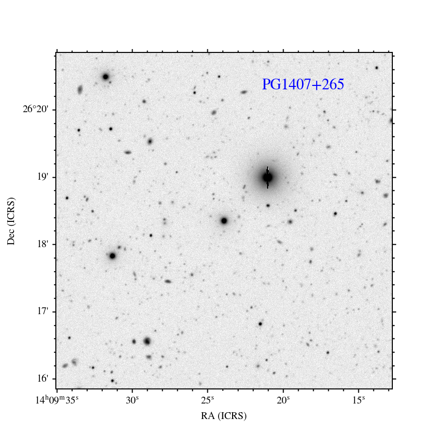
Figure 1: $V$-band image of the field surrounding PG1407+265 (centered) obtained with the LBC on the LBT. [See the Journal version for the full image.]

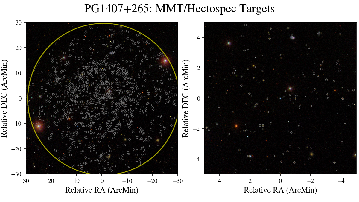
Figure 2: Illustration of the targeting strategy for Hectospec observations of the PG1407+265 field. The left panel shows the entire Hectospec field-of-view, centered on PG1407+265. Note the ‘wedding cake’ strategy employed, i.e., a denser set of targets closer to the quasar. The right-hand panel shows a zoom-in to illustrate the depth of targeting. [See the Journal version for the full image.]

2.3 Targeting

2.3.1 Hectospec

From the SDSS imaging data described above, we generated target lists to observe with the MMT/Hectospec spectrograph employing a ‘wedding-cake’ strategy that sampled the inner angular offsets from the quasar to fainter magnitudes. Specifically, we targeted galaxies with $r<22$ mag for $\theta<5^{\prime}$, $r<21$ mag for $\theta=[5^{\prime},10^{\prime}]$, and $r<20$ mag to $\theta=30^{\prime}$. This was done because at lower redshifts, it is desirable to cover a larger FOV to probe similar impact parameter ranges as the higher redshift data, but the survey does not need to go as deep as the higher$-z$ observations to reach similar galaxy luminosities.

Figure 2 shows an example of target selection taken from the PG1407+265 field and Figure 3 presents the completeness for all of the fields with the wedding-cake criteria above. The targeting completeness reported here is the percentage of targets with a fiber placed upon them during our observing runs. Details on the spectroscopy and redshift determinations are provided in the following section.

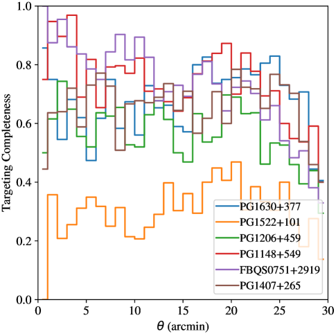
Figure 3: Completeness fraction for the targeting of galaxies (i.e., fraction of fibers on desired galaxies for Hectospec only) selected from SDSS imaging according to our targeting criteria. The value is independent of whether a precise redshift was measured from the resultant spectrum. Note that the sparsest field (PG1522+101) was observed with only 2 configurations.

2.3.2 DEIMOS

With Keck/DEIMOS, we pursued fainter galaxies that are more effectively surveyed with this telescope/instrument combination, which has a smaller field-of-view but also a larger primary mirror. For these observations, we again gave higher priority to sources close to the quasar (in angular offset) but had additional, observing-related criteria that further affected our slit-mask designs. Figure 4 illustrates the targeting for the PG1407+265 field, where we adopted the following criteria: (1) $\theta<15^{\prime}$, (2) $14<V<24.5$, and (3) SExtractor star-galaxy classifier $S/G<0.9$, except for sources within $20^{\prime\prime}$ of the quasar where no S/G criterion was applied. Other fields had small differences from these criteria, as summarized in Table 4.

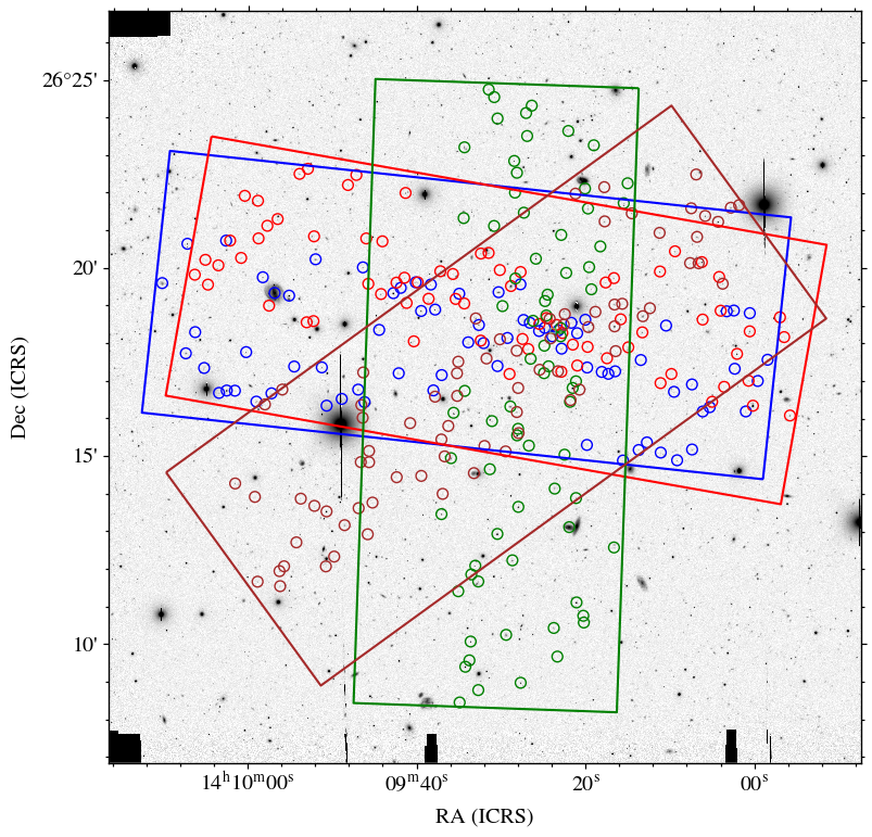
Figure 4: Slitmask FOVs (rectangles) and associated targets (circles) for the PG1407+265 field observed with Keck/DEIMOS. This quasar is surrounded by the densest distribution of targets among those in our survey. [See the Journal version for the full image.]

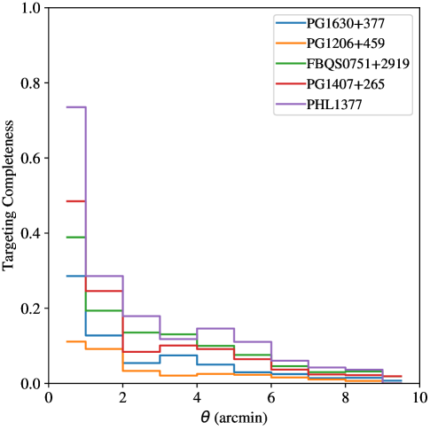
Figure 5: Completeness of targeting for the fields observed with Keck/DEIMOS defined as the fraction of targets observed. The value is independent of whether a precise redshift was measured from the resultant spectrum.

In general, we avoided targeting sources previously observed by SDSS or our own Hectospec program. Similar to Figure 3, Figure 5 shows the completeness for the DEIMOS fields. In contrast to the Hectospec survey, the DEIMOS survey has sparser coverage and higher incompleteness which resulted mainly from poor weather.

Table 4: DEIMOS Targeting Criteria

Field	Filter	S/G${}^{a}_{\rm max}$	$m_{\rm max}^{b}$	$\theta_{\rm max}^{c}$
PG1630+377	R	0.9	25.0	15.0
PG1206+459	V	0.9	25.0	15.0
FBQS0751+2919	V	1.0	24.5	10.0
PG1407+265	V	0.9	24.5	15.0
PHL1377	V	1.0	24.5	15.0

Table 5: Hectospec Observing

Field	Configuration	Date	Total Exposure
			sec
FBQS0751+2919	1	2011 Jan 25	5400
FBQS0751+2919	2	2011 Jan 26	5400
FBQS0751+2919	3	2011 Feb 10	5400
FBQS0751+2919	4	2011 Mar 25	5400
PG1148+549	1	2011 Feb 10	5400
PG1148+549	2	2011 Feb 11	5400
PG1148+549	3	2011 Feb 11	5400
PG1148+549	4	2011 Mar 30	7187
PG1206+459	1	2012 Jan 21	3600
PG1206+459	2	2012 Mar 14	3600
PG1206+459	3	2012 Feb 22	3600
PG1407+265	1	2011 Jun 03	3600
PG1407+265	2	2011 Jun 03	3600
PG1407+265	3	2011 Jun 05	3600
PG1407+265	4	2011 Jun 06	3600
PG1522+101	1	2011 Jun 05	3600
PG1522+101	2	2012 Feb 22	3600
PG1630+377	1	2011 Jun 03	3600
PG1630+377	2	2011 Jun 04	2700
PG1630+377	3	2011 Jun 05	3120
PG1630+377	4	2011 Jun 06	3600

Table 6: DEIMOS Spectroscopic Observations

Field	Mask ID	Nslitlets	Date Obsa
PHL1377	M1-8005	88	2012 Nov 14
PHL1377	M2-8006	87	2012 Nov 14, Dec13
PHL1377	M3-8007	86	2012 Nov 14
FBQS0751+2919	M4-8008	87	2012 Nov 14, Dec 13
FBQS0751+2919	M5-8009	93	2012 Dec 13
PG1206+459	M1-8377	72	2013 May 07, 08
PG1407+265	M1-8380	75	2013 May 07, 08
PG1407+265	M2-8381	74	2013 May 08
PG1407+265	M3-8382	74	2013 May 08
PG1407+265	M4-8383	76	2013 May 07, 08
PG1630+377	M3-8387	69	2013 May 07
PG1630+377	M4-8388	75	2013 May 08

3 Spectroscopy

3.1 Observations

3.1.1 Hectospec

For all of the Hectospec data collected in our CASBaH survey, we employed an identical setup of 300 1.5^′′ fibers and the G270 grating, yielding $R\approx 1,000$ with wavelength coverage $\lambda_{\rm ob}\approx 3,700-9,200$Å. The observations used three or more exposures with times ranging from 900s to 1800s each, for a total exposure of 3600s or 5400s as detailed in Table 5. Each fiber configuration included $\sim$ 20 fibers placed on ‘blank’ sky.

All of these spectra were reduced by the HSREDv2 data reduction pipeline to wavelength calibrate, extract, sky subtract, and flux the fiber data. The $1\sigma$ error array assumes Gaussian statistics and a 2 electron read noise term. Each exposure was reduced separately, and the final 1-D spectra were co-added in wavelength space weighted by the inverse variance of the individual exposures. The pipeline, in our case, produced a wavelength solution calibrated in air and unfluxed. Therefore, we converted to vacuum with the Ciddor equation described at NIST. The spectra were fluxed using a sensitivity function derived from Feige 34 observed on another program. We caution that the absolute fluxes do not include corrections for fiber losses, airmass, telluric absorption or variable observing conditions.

Figure 6 shows several examples of spectra for sources spanning the dynamic range of observed magnitudes ($r\approx 18.1-21.9$ mag). The median S/N of all spectra is approximately 5.3 per 1.2Å pixel at $\lambda_{\rm ob}\approx 5,000$Å.

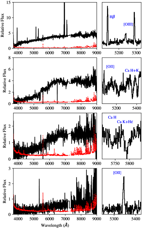
Figure 6: Representative spectra from the Hectospec observations. Cut-outs on the right show examples of key spectral features used in the redshift determination.

3.1.2 DEIMOS

For the DEIMOS observations of the CASBaH target fields (Table 6), we designed slitmasks with the DSIMULATOR software taking into account atmospheric dispersion with an attempt to optimize targets and observing time. We employed the G600 grating, which yields a spectral resolution $R\approx 1600$ for our $1^{\prime\prime}$ slits, a dispersion of $\approx 0.5$Å per pixel, and an approximate wavelength coverage of $\lambda_{\rm ob}\approx 5,000-10,000$Å. The spectral images include arc and quartz lamp calibration frames. All of these data were reduced with the spec2d data reduction pipeline developed by M. Cooper for the DEEP survey (Newman et al., 2013). The pipeline produces optimally extracted, wavelength-calibrated spectra (in air and converted later to vacuum). Multiple exposures taken with a given mask on the same night are combined in 2D by the DRP. Masks exposed on separate nights were extracted separately and the individually, extracted 1D-spectra were coadded with a custom algorithm.

From observations of two spectrophotometric standards, Feige 110 and 34, on three separate nights, November 14, 2012, December 13, 2012 (Feige 110), and May 8, 2013 (Feige 34) we generated a combined sensitivity function that was applied to the entire CASBaH DEIMOS spectroscopic dataset. Again, we made no correction for slit losses, airmass, or variable observing conditions. Furthermore, vignetting at the edges of the detector leads to fluxing error at the longest and shortest wavelengths.

Representative spectra spanning the dynamic range of sources observed with DEIMOS are illustrated in Figure 7. The median S/N of the complete dataset at $\lambda_{\rm ob}\approx 6,500$Å is $\approx 2.9$ per 0.6Å pixel.

The standard mode of the spec2d extraction algorithm searches for additional sources in each slit (in part to assist sky subtraction) and extracts them. We have used the mask information and our astrometry to assign each an RA and DEC coordinate. Where possible, we have also matched them to our photometric catalog. All of these ‘serendipitous’ spectra are included in the database and were analyzed in a similar manner as the primary targets.

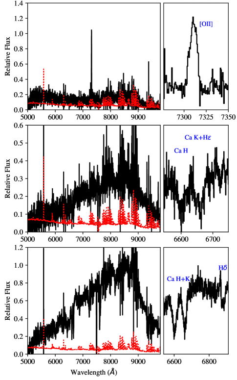
Figure 7: Gallery of example spectra from the Keck/DEIMOS observations, ordered from top to bottom by increasing flux. Cut-outs on the right show examples of key spectral features used in the redshift determination.

3.2 Redshift Analysis

Redshift analysis proceeded in two stages. The first stage employed a template-fitting algorithm custom to the spectrograph (see following sections). These results were vetted by one or more co-authors and a quality flag $Z_{Q}$ was assigned to each source with $Z_{Q}=0,1,2,3,4$ as follows: (0) Data too poor for any assessment; (1) Data poor and redshift highly uncertain; (2) Data quality good but no redshift determined; (3) Data quality good and redshift is highly likely but not confirmed by multiple lines (or one line is of low S/N); (4) Highly certain and confirmed by multiple spectral features (see also Newman et al., 2013). We then analyzed each spectrum with the RedRock software package v0.7, which is under development by the Dark Energy Spectroscopic Instrument project. This code also compares a set of galaxy and star templates to the spectra to generate a set of best-fitting models and corresponding redshift estimates. We then inspected every RedRock solution offset by more than $50{\rm\;km\;s^{-1}}$ from the original estimate and resolved the conflict based on the observed spectral features (if any). Only sources with $Z_{Q}\geq 3$ are considered reliable. We now detail specific aspects of the analysis and results for each instrument.

3.2.1 Hectospec

The first algorithm adopted for Hectospec redshift calculation is a modified version of zfind developed by the SDSS project, which cross-correlates a series of templates (stars, galaxies and quasars) in measurement space (i.e., no Fourier transform is applied). These are then ranked in $\chi^{2}$ and the lowest value is selected by the redshift code. Figure 8 summarizes the fraction of sources with $Z_{Q}\geq 3$ as a function of observed magnitude. For $r<21$ mag, the redshift success rate exceeded 95% and, as expected, declined with fainter sources. Nevertheless, the success rate remains high to the magnitude-limit of the survey.

Spectra that showed redshift discrepancies of the order of 50${\rm\;km\;s^{-1}}$ between the RedRock and Hectospec solutions were visually inspected, and the solution that showed the best matching locations of certain prominent galaxy lines was selected. We found that the majority of cases favored the RedRock determination, though in cases where the S/N was low, the Hectospec/zfind determination frequently showed the higher confidence redshift.

The reported redshift uncertainty from these $\chi^{2}$-minimization codes is frequently several times $10^{-5}$, i.e., $\sigma_{v}\approx 10{\rm\;km\;s^{-1}}$. We consider such small errors to be overly optimistic and suggest one assume a minimum of $30{\rm\;km\;s^{-1}}$ uncertainty due to systematic error (e.g., wavelength calibration).

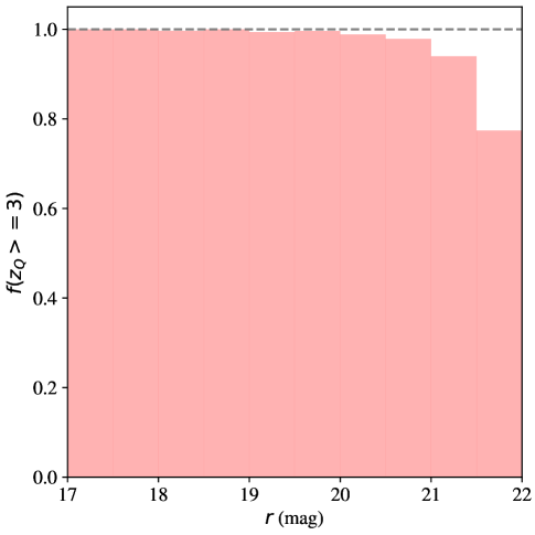
Figure 8: Redshift completeness fraction for sources observed with Hectospec as a function of $r$ magnitude.

3.2.2 DEIMOS

For the DEIMOS spectra, we derived redshifts with two separate algorithms with two different sets of co-authors: (i) a modified version of the SDSS zfind algorithm by JW and SL and (ii) the RedRock software package v0.7 developed by the DESI experiment. For nearly 500 sources, the two packages reported redshifts that matched to within $50{\rm\;km\;s^{-1}}$. For these we simply adopted the RedRock estimate and assigned $Z_{Q}=3$. For all other cases (approximately 600 sources, the majority of which had no previously determined redshift), we vetted each of these manually. After visually inspecting the spectra, we assigned the solution with coincident, prominent spectral features. In a few percent of the cases, we assigned a redshift of our own estimation. This included most of the galaxies at $z>1$ because we had limited our automatic search to less than this redshift.

Figure 9 shows the redshift measurement success rates from our DEIMOS analysis where a secure redshift is defined with $Z_{Q}\geq 3$. This analysis is limited to the primary targets, i.e., we ignore serendipitous sources that entered the DEIMOS slits. The success rate is approximately 95% to 22 mag, declines to $\approx 80\%$ at 24 mag, and drops rapidly from there.

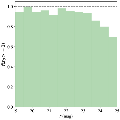
Figure 9: Redshift success rate for sources observed with DEIMOS as a function of $r$ magnitude.

3.3 Galaxy Spectroscopy Summary

Integrating the redshift measurements from Hectospec, DEIMOS, and the SDSS database, we performed internal comparisons between the $\sim 175$ sources common to two or more of the sub-surveys. Ignoring catostrophic failures (described below), the measured RMS values between Hectosec/SDSS and DEIMOS/Hectospec are $\approx 35{\rm\;km\;s^{-1}}$ and $\approx 36{\rm\;km\;s^{-1}}$ respectively. Therefore, we advise one adopt a minimum redshift uncertainty of $35{\rm\;km\;s^{-1}}$ for galaxies drawn from the CASBaH database. We find no variation with emission/absorption-line properties among this common set of galaxies. This exercise also revealed 13 cases where the recovered redshifts were substantially offset ($\delta v\gg 100{\rm\;km\;s^{-1}}$). In nearly all of the cases, at least one of the two spectra was of poor data quality. All but one of the non-SDSS spectra already showed $Z_{Q}<3$ and we have now downgraded the few from SDSS accordingly. In two cases, there were multiple sources with separation $<1^{\prime\prime}$ in the slit/fiber; we have corrected the catalog accordingly.

The CASBaH spectroscopic redshift survey is summarized in Table 7. Altogether in the 9 fields, we have 5902 galaxies with high quality redshifts ($Z_{Q}\geq 3$) and $z_{\rm em}>0.00166$. Their redshift distribution is shown in Figure 10 for the three primary datasets of our program. Clearly, our Hectospec survey provides the majority of spectroscopic redshifts. These lie predominantly at $z_{\rm em}=[0,0.5]$. The DEIMOS dataset contributes primarily at $z_{\rm em}>0.5$, as designed. We also report 356 sources with $Z_{Q}<3$ and no secure redshift measured as well as 279 spectra from DEIMOS and Hectospec of stars.

With our adopted cosmology, we may translate the galaxy redshifts and their angular offsets from their corresponding quasar sightline to estimate the impact parameter (physical $R_{\rm phys}$ and comoving $R_{\rm com}$). The distributions on small ($R_{\rm phys}<450$ kpc) and large ($R_{\rm com}\sim 10$ cMpc) scales are summarized in Figure 11. These distributions show the statistical power of CASBaH for studies of the CGM and IGM, respectively.

Table 7: CASBaH Redshift Survey^a

CAS_ID	RA	DEC	$z_{\rm em}$	$\sigma(z)^{b}$	ZQ	Instr.
4494	212.37009	26.32546	0.3273	0.0001	4	SDSS
4495	212.38848	26.47184	0.2964	0.0001	4	SDSS
4496	212.31438	26.36133	0.0000	0.0001	3	Hectospec
4497	212.45230	26.21947	0.5490	0.0001	3	Hectospec
4498	212.39738	26.31966	0.8081	0.0001	3	Hectospec
4499	212.38745	26.31115	0.3975	0.0001	3	Hectospec
4500	212.46825	26.34760	0.4230	0.0001	4	Hectospec
4501	212.25992	26.31462	0.3698	0.0001	3	Hectospec
4502	212.28271	26.31439	0.0000	0.0001	3	DEIMOS
4503	212.45042	26.33128	0.0000	0.0001	3	DEIMOS
4504	212.46587	26.30656	0.0000	0.0001	3	DEIMOS
4505	212.47700	26.31067	0.0000	0.0001	3	DEIMOS
4506	212.35095	26.31103	-1.0000	0.0001	0	DEIMOS
4507	212.28904	26.34083	0.4264	0.0001	3	DEIMOS
4508	231.20121	9.91829	0.6041	0.0002	3	SDSS
4509	231.19939	9.93566	0.1518	0.0001	3	SDSS

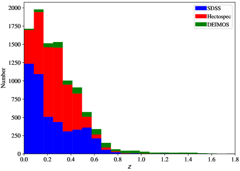
Figure 10: Histogram of the galaxy redshifts from the three main sources for the CASBaH survey: SDSS, Hectospec, and DEIMOS. The histograms are stacked, not overlapping, i.e., the DEIMOS histogram is placed above Hectospec.

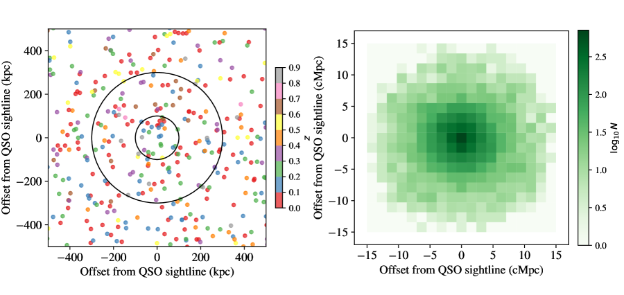
Figure 11: Distributions of galaxies around the quasar sightlines of CASBaH on small-scales (left), which probe the circumgalactic medium of the galaxies and on large scales (right), which trace the distribution of the intergalactic medium. Annuli in the left panel indicate impact parameters of 100 kpc and 250 kpc.

4 Derived Quantities

The previous sections described measurements made (nearly) directly from the imaging and spectroscopic data. This section describes a few quantities derived from the combined measurements, e.g., two or more filters and/or a combination of photometry and spectroscopy. We generally adopt standard techniques, assumptions, and software in the analysis and warn that the uncertainties (especially systematic error) can be large.

4.1 SED Fitting

To estimate the stellar masses and SFRs of all galaxies in our database, we have employed our spectroscopic redshifts, the photometric measurements from our own LBT/LBC observations, and photometry from various publicly available survey catalogs spanning the optical and near-infrared. We fit the spectral energy distributions (SEDs) of each galaxy with stellar population model spectra, models for dust attenuation, and emission from nebular lines using the CIGALE software package (Noll et al., 2009). While myriad high-quality SED fitting codes are available, we chose CIGALE for several reasons, including its ability to easily handle our heterogeneous dataset given the variety of sources from which our data are derived (e.g., certain fields were covered by a given survey while others were not, and within a field, not all objects were detected in a single survey). Furthermore, CIGALE natively supports several choices for stellar-population models, dust models, etc., across a wide range of parameters. We discuss our choices for these parameters below so that the reader may recreate or improve upon our estimates.

We assembled our photometric dataset for SED fitting by cross-matching all galaxies in our spectroscopic database having redshift quality scores $Z_{Q}\geq 3$ with several public survey catalogs: SDSS DR12 (Alam et al., 2015, $ugriz$ coverage of all fields except PHL1377), the Canada-France-Hawaii Telescope Legacy Survey (CFHTLS; Hudelot et al., 2012, $ugriz$ coverage of the PHL1377 field), the Wide-field Infrared Survey Explorer all sky survey (Cutri & et al., 2013, 3.4, 4.6, 12, and 22 $\mu$m bands for all fields), BASS (Zou et al., 2017b, a), UKIDSS (Warren et al., 2007; Lawrence et al., 2007), KiDS (de Jong et al., 2017), DECALS (Dey et al., 2018), MzLS (Dey et al., 2018), and Pan-STARRS (Flewelling et al., 2016; Chambers et al., 2016).

We then corrected all magnitudes for Galactic reddening using the (Schlafly & Finkbeiner, 2011) extinction values provided by the Nasa Extragalactic Database service accessed through the astroquery framework. Reddening values are returned for a limited number of filter bandpasses (UBVRIugrizJHKL’), and we dereddened our photometry data using those most closely matching the central wavelengths of filters used in our compiled dataset. CIGALE integrates fitted stellar population models over any filter response curve provided; we employed the SVO Filter Profile Service (Rodrigo et al., 2012) as well as individual survey websites to obtain filter curves and zeropoints corresponding to each band.

As mentioned above, CIGALE includes a variety of models to include in the fitting. For stellar populations, we used the Bruzual & Charlot (2003) models, assuming a Chabrier (2003) initial mass function, with metallicities ranging from $<1/100$th solar to 2.5x solar. The star formation histories included in our models (via the ‘sfhdelayed’ module) spanned 0.25-12 Gyr for the oldest population with e-folding times 0.1-8 Gyr. In addition to the stars, we included nebular emission with the default values and reprocessed dust emission using the Dale et al. (2014) model with slopes $\alpha=1-2.5$ and 0% AGN fraction.

The final component of our modeling is the dust attenuation curve, for which we adopted a model based on that of Calzetti et al. (2000) but also includes a ‘bump’ in the UV. The Calzetti et al. (2000) form, although originally derived for starburst galaxies, was later validated by Battisti et al. (2016) for local star forming galaxies more generally, and Battisti et al. (2017) found evidence for a bump feature in inclined galaxies. We adopt the modification by Buat et al. (2011) and implemented in CIGALE by Buat et al. (2011) and Lo Faro et al. (2017) with 35.6 nm and 217.5 nm the bump width and wavelength, respectively. The bump amplitude setting is 1.3, and the slope is modified by $-0.38$. We reduce the color excess of old population relative to the young stars by a factor of 0.44 and allow the $E(B-V)$ for the young population to vary between 0.12 and 1.98.

4.2 Stellar Mass, SFR, and Rest-frame Color

Once each galaxy’s SED has been fitted, a number of physical parameters as well as the rest-frame absolute magnitudes are then extracted from the resulting stellar population models. Figures 12-14 illustrate the measurements gleaned from SED fitting for the complete CASBaH galaxy database. As shown in Figures 12 and 13, the locus of measured stellar masses spans from $M_{*}\approx 10^{8}-10^{11}M_{\odot}$ with a median $\bar{M}_{*}\approx 10^{10.1}M_{\odot}$. at $\bar{z}=0.28$. These values are driven by our Hectospec sample. The SFRs in Figure 13 show that the majority of our galaxies are star-forming. We have compared our results to measurements for other $z<1$ surveys (e.g., PRIMUS; Moustakas et al., 2013) and find similar results. Lastly, the color-magnitude diagram (Figure 14 reveals the bimodal populations of star-forming and red-and-dead galaxies. In summation, the basic measured properties of galaxies discovered in our survey reproduce/follow the typical trends and distributions characteristic of any other low-$z$ sample.

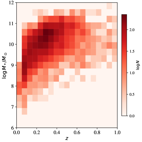
Figure 12: Distribution of stellar mass vs. redshift for the spectroscopically confirmed galaxies comprising the CASBaH sample. The median of the sample occurs at $\bar{z}=0.28$ and $\bar{M}_{*}\approx 10^{10.1}M_{\odot}$.

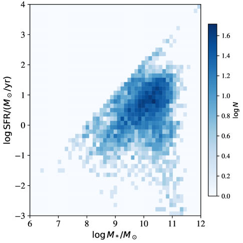
Figure 13: SFR vs. stellar mass from SED fitting for the CASBaH galaxy sample, where one well recognizes the locus of galaxies known as the star-forming main-sequence. The hard diagonal edge at the highest SFR for each stellar mass bin occurs due to failures/outliers fitted with models at the boundaries of parameter space.

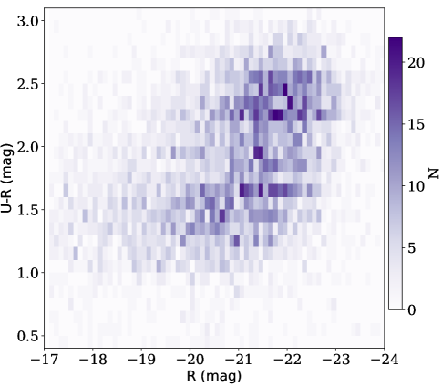
Figure 14: Color-magnitude diagram (rest-frame) for galaxies comprising the CASBaH sample. Evident is the well-known bimodal populations of star-forming and ‘red-and-dead’ galaxies.

5 Identification and Measurement of O VI Absorbers

In the following section, we will study the study the clustering of O VI absorbers with galaxies using the CASBaH database. The full description of the CASBaH ultraviolet QSO spectroscopy and data handling is presented in Tripp et al. (2019, in prep.); in this section, we summarize aspects of the O VI identifications and measurements that are important for the absorber sample definition and O VI-galaxy clustering analysis.

We identified the O VI absorption lines using the multipass line-identification procedure described by Tripp et al. (2008). In the first pass through the data, we simply searched for lines with the signature of the O VI doublet, i.e., lines with the relative separation and relative strengths of the O VI 1031.926 and 1037.617 Å transitions (see, e.g., Verner et al., 1994). In this pass, we did not require detection of any corresponding H I or metal lines; we only searched for the O VI doublet by itself. This first pass identified the majority of the O VI absorbers, but in some cases, evidence of blending with lines from other redshifts was clearly evident. This is not surprising given the moderately high density of lines in the CASBaH QSO spectra (see Fig. 1 in Tripp, 2013). In addition, in some cases, one line of the doublet is so severely blended with a strong feature from a different redshift that both lines of the doublet could not be directly recognized in our first pass through the data. To overcome these blending issues, we iteratively made subsequent passes through the spectra in which we added information about absorption systems established by the presence of H I lines (often with many lines of the Lyman series) and various metals. CASBaH absorbers often show many metal and H I lines with distinctive component structure (e.g., Tripp et al., 2011; Ribaudo et al., 2011a; Lehner et al., 2013; Meiring et al., 2013), and we used the detailed correspondence of candidate O VI lines with other metals at the same redshift to identify additional O VI absorbers when one or both of the O VI lines was affected by blending (for examples with Ne VIII lines, see Burchett et al., 2018). Since the CASBaH spectra fully cover the H I Ly$\alpha$ region from $\lambda_{\rm ob}$ = 1216 to $(1+z_{\rm QSO})\times 1216$, we are able to identify nearly all of the lines and systems in the spectra (not just the O VI systems), including the lines that are blended with the O VI doublets. Often the interloping lines that are blended with an O VI absorber can be modeled and removed based on lines recorded elsewhere in the CASBaH spectra, and then comparison of the deblended data further corroborates the identification.

In this paper, we are only interested in the foreground/intervening absorption systems (far from the background QSOs) and their relationships with foreground galaxies. To avoid contaminating our intervening-absorber sample with “proximate” ($z_{\rm abs}\approx z_{\rm QSO}$) absorbers that often comprise material ejected by the QSO that is close to the QSO’s central engine (Misawa et al., 2007; Ganguly et al., 2013), we exclude O VI absorbers within 5000 km s^-1 of the QSO redshift.

All of the intervening O VI absorbers that we identify exhibit H I absorption at very similar velocities and often show other metal lines (at least C III or O IV, and often other metals); we do not find any unambiguous O VI systems without any corresponding H I. This is consistent with previous studies of low-redshift O VI absorbers, which have shown that the “H I-free” O VI systems are only found in proximate cases with $z_{\rm abs}\approx z_{\rm QSO}$ (Tripp et al., 2008). We note that some intervening O VI systems have interesting individual O VI components that have corresponding H I that is very weak (or absent altogether, see, e.g., Tripp et al., 2008; Savage et al., 2010), but these cases are not H I-free; on the contrary, these absorbers have very strong corresponding H I absorption in some of the components of the overall system. For example, Savage et al. (2010) have analyzed the O VI system at z = 0.167 in the spectrum of PKS0405-123. This system includes an O VI component at $v=-278$ km s^-1 that is not detected in H I, but the same system also shows O VI components at $v\approx-125,-50,$ and 0 km s^-1, and these lower-velocity components have strong corresponding H I absorption (see Fig.3 in Savage et al., 2010). Thus, this example has an H I-free component, but it is not an H I-free system; similar intervening systems are found in the CASBaH database. Only the proximate absorption systems are entirely free of H I in all of the components (some examples of such proximate systems are shown in Fig.7 and Fig. 20 of Tripp et al., 2008).

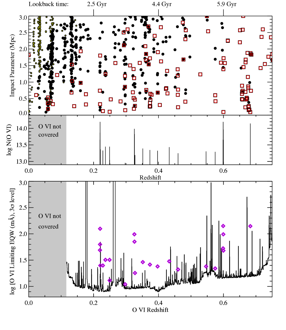
Figure 15: Top: Galaxies in the CASBaH database for PG1407+265 as a function of redshift, within impact parameters of 3 Mpc or less at $z_{\rm gal}<0.75$. Galaxies with redshifts from SDSS are indicated by small circles with yellow centers, galaxy redshifts measured with Hectospec are represented with larger filled-black circles, and galaxies measured with DEIMOS are shown with red squares. For reference, lookback times are indicated on the top axis. Middle: logarithmic column densities and redshifts of the O VI absorption lines detected in the UV spectra of PG1407+265. Each vertical line marks the redshift of an O VI component, and the height of the line indicates log $N$(O VI). Bottom: The 3$\sigma$ limiting equivalent width for detection of O VI in the PG1407+265 data vs. redshift. The equivalent widths of detected O VI components are plotted with purple diamonds.

To measure the absorption-line properties, here we primarily rely on fitting multicomponent Voigt profiles to the data using the software developed by Burchett et al. (2015). These models constrain the redshift, line width, and column density of each O VI component, and we aggregate the components into “systems” as described below. To assess the significance of the candidate lines, we use the Voigt-profile parameters to calculate the equivalent width, which we then compare to the limiting equivalent width (calculated using the method of Tripp et al., 2008) at that wavelength. In this paper we have focused on well-detected lines ($>4\sigma$ significance) that are not involved in very complicated blends that preclude robust profile fitting. In this conservative sample, we find a paucity of lines with log $N$(O VI) $<$ 13.5, and we also impose a lower limit on the O VI column density of absorbers that are included in the clustering analysis (see below).

Figure 15 provides a snapshot of the overall database (galaxy and O VI absorber information) using the PG1407+265 sight line and field as an example. In the top panel of this figure, we show the full galaxy database in a cylinder with radius = 3 Mpc centered on the QSO. The middle panel illustrates the column densities of the O VI lines are their locations with respect to the nearby galaxies and large-scale structures that can be seen in the upper panel, and the lower panel shows the 3$\sigma$ limiting (rest-frame) equivalent width as a function of O VI redshift with the equivalent widths of the detected O VI lines overplotted. Comparing the O VI and galaxy impact parameters, we see that O VI lines are typically detected when there is a galaxy close to the line of sight, but there is substantial scatter in the O VI column at a given impact-parameter value. This is consistent with previous studies (e.g., Stocke et al., 2006; Tumlinson et al., 2011; Johnson et al., 2015). We will present analyses of the connections of individual O VI-galaxy papers in a separate paper (Burchett et al., in prep.). We also see from Figure 15 that the CASBaH database provides extensive information on galaxy structures on large scales, which is the focus on the galaxy-absorber analyses in this paper.

6 OVI-Galaxy Clustering

With the galaxy spectral database of CASBaH constructed, we proceed to measure the clustering of CASBaH galaxies with themselves (auto-correlation) and with O VI absorption systems (cross-correlation) in the $z<1$ Universe. Our scientific motivations are two-fold: (i) to further characterize the galaxy sample of the CASBaH survey; and (ii) to provide new estimates on the masses of galaxies associated with O VI absorption. Regarding the latter goal, we emphasize that the results derived will only apply for O VI systems with properties similar to those drawn from CASBaH. Furthermore, any estimate on mass follows from the ansatz that the majority of these O VI systems arise within dark matter halos. We also emphasize that incompleteness in the galaxy and O VI samples is accounted for by the estimator and procedures adopted in the clustering analysis. Last, we restrict the analysis to comoving separations in excess of $1h_{100}^{-1}\,{\rm Mpc}$ to isolate the so-called two-halo term that results from large-scale clustering.

6.1 Setup

This sub-section describes cuts on our absorber and galaxy databases used to generate a well-defined set of systems and galaxies for the analysis. To measure O VI-galaxy clustering, we define a discrete set of O VI systems along the sightlines, with each system characterized by a systemic redshift $z_{\rm sys}$ and column density ${N({\rm OVI})}$. To achieve this, our approach in this CASBaH paper is to synthesize components (provided by Tripp et al., 2019) into absorption systems. Using the MeanShift clustering algorithm from the scikit-learn Python package (Pedregosa et al., 2011), we grouped components clustered in velocity space into absorption systems, setting the redshift of each system to the center of its component cluster. The MeanShift algorithm accepts a ‘bandwidth’ argument, which defines an approximate width within which to group components. We chose a bandwidth value of 600 ${\rm\;km\;s^{-1}}$ for component clustering, finding that this value was large enough to produce systems with components spread over a large range of velocity ($\sim 1000$ ${\rm\;km\;s^{-1}}$), such as the post-starburst outflow analyzed by Tripp et al. (2011), but small enough to separate systems with components clustered about discrete center points with large separations (also on the order of 1000${\rm\;km\;s^{-1}}$). For systems composed of multiple components, we sum their individual column densities to yield a total ${N({\rm OVI})}$ for each system.

These values are shown in Figure 16 as a function of system redshift. At $z<0.75$, the sample scatters from ${N({\rm OVI})}\approx 10^{13.3}-10^{14.5}$ with no discernible redshift evolution (the cut-off at $z\approx 0.12$ is due simply to lowest observed wavelength of our FUV spectra, $\lambda_{\rm ob}$ = 1152 Å). At higher redshifts, the ${N({\rm OVI})}$ values are systematically higher (see discussion in Tripp et al., 2019). These issues motivate sample criterion 1: the clustering analysis is restricted to $0.12<z<0.75$. This criterion is also motivated by the small number of galaxies that we have observed at higher redshift (e.g., Figure 10).

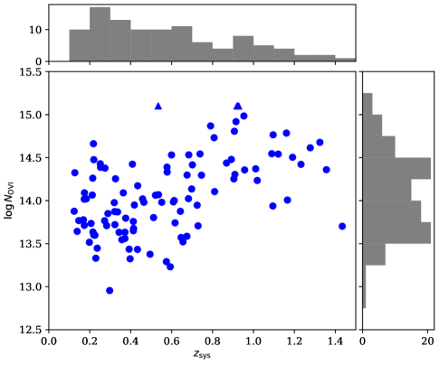
Figure 16: Scatter plot and histograms of the column densities versus redshift for the O VI systems detected in the CASBaH survey. Typical uncertainties in ${N({\rm OVI})}$ are $\approx 0.03$ dex. The measurements with ${N({\rm OVI})}>10^{15}\,{\rm cm^{-2}}$ are saturated, are reported as lower limits, and are designated with triangles. The lack of of weaker O VI absorbers at $z>0.75$ is driven by the shift of the O VI doublet from the FUV to the NUV bandpass where the spectra have lower signal-to-noise levels.

Further examining the O VI column density histogram, one notes a marked decline in the number of systems with $\log{N({\rm OVI})}<13.5$; e.g.,  only one system exhibits $\log{N({\rm OVI})}<13.2$. We emphasize that this dropoff is not entirely driven by sensitivity. Indeed, a substantial fraction of the CASBaH FUV spectra have a $2\sigma$ limit on ${N({\rm OVI})}$ that is lower than $10^{13.5}\,{\rm cm^{-2}}$ (for O VI $\lambda$1031 over an integration window of $60{\rm\;km\;s^{-1}}$). Therefore, the observed distribution implies a physical turn-over in the ${N({\rm OVI})}$ frequency distribution as also reported by Danforth et al. (2016); this will be explored further in a future manuscript. For the clustering study, we are motivated to set a minimum column density threshold ${N({\rm OVI})}_{\rm lim}$ for including O VI systems in the analysis. This provides a well-defined sample and we can set ${N({\rm OVI})}$ to be sufficiently high to include nearly all of the COS-FUV data. We find that ${N({\rm OVI})}_{\rm lim}=10^{13.5}\,{\rm cm^{-2}}$ satisfies this goal and also includes the majority of O VI systems detected; this motivates sample criterion 2: We restrict the O VI systems to those with ${N({\rm OVI})}\geq{N({\rm OVI})}_{\rm lim}$. The primary exceptions to an approximately uniform sensitivity in the COS-FUV spectra are spectral regions absorbed by other, unrelated systems (e.g., Lyman series absorption by a system at higher redshift). For each galaxy at $0.12<z<0.75$, we have assessed the spectra in a $\pm 30{\rm\;km\;s^{-1}}$ window centered at the O VI $\lambda$1031 wavelength and find that $\approx 16\%$ have a significant blend that prohibits sensitivity to ${N({\rm OVI})}_{\rm lim}$. This motivates sample criterion 3: We ignore galaxies whose redshift places them in a blend that prohibits measuring down to ${N({\rm OVI})}_{\rm lim}$, despite the overall high S/N of the spectra.

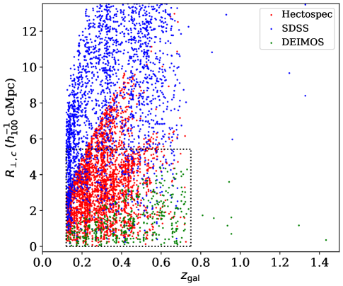
Figure 17: Scatter plot of the comoving impact parameter $R_{\perp,c}$ versus galaxy redshift for the $\approx 6,000$ galaxies that have redshifts corresponding to CASBaH absorption data that are sufficiently sensitive to detect an O VI system with ${N({\rm OVI})}\geq 10^{13.5}\,{\rm cm^{-2}}$. The dotted box illustrates the $R_{\perp,c}$,$z_{\rm gal}$ parameter space used for our OVI-galaxy cross-correlation analysis.

Figure 17 illustrates the set of galaxies satisfying the three sample criteria, plotted at their comoving distance from the quasar sightline. To enforce the ${N({\rm OVI})}_{\rm lim}$ criterion, we estimated the uncertainty in column density by integrating the apparent optical depth at O VI $\lambda$1031 in a window of $\pm 30{\rm\;km\;s^{-1}}$ centered on each galaxy redshift. We then flagged those with $2\sigma({N({\rm OVI})})<10^{13.5}\,{\rm cm^{-2}}$, without a blend, and with $z_{\rm gal}>0.12$. Altogether we have $\approx 6,000$ galaxies in the CASBaH survey satisfying these criteria. It is apparent from Figure 17 that very few galaxies with $z_{\rm gal}>0.75$ have sufficient S/N at O VI to satisfy the sensitivity limit (see also Tripp et al., 2019). One also notes that, at fixed redshift, the CASBaH survey has a roughly constant galaxy sampling to $R_{\perp,c}\approx 5.4\,\rm h_{100}^{-1}cMpc$ which declines monotonically with increasing $z_{\rm gal}$. Beyond $R_{\perp,c}\approx 5.4\,h_{100}^{-1}\,{\rm Mpc}$, one identifies striping related to the wedding cake design of the Hectospec observations ($\S$ 2.3.1). This leads to sample criterion 4: restrict the cross-correlation analysis to $R_{\perp,c}<5.4\,h_{100}^{-1}\,{\rm Mpc}$.

Lastly we restrict the analysis to the 7 fields observed with Hectospec, DEIMOS, or both (i.e., PG1338+416 and LBQS1435$-$0134 are not used in this paper). The fields with only SDSS coverage have too few galaxies (i.e., too large shot noise) for a meaningful analysis.

6.2 Galaxy-Galaxy Auto-correlation

Interpretation of the results from the O VI-galaxy cross-correlation analysis will depend on the nature of the galaxies that comprise the CASBaH survey. We have assessed several intrinsic properties in the previous section (e.g., Figure 12); here we perform an auto-correlation analysis to further assess the halo mass of the population.

Our methodology follows closely that of Tejos et al. (2014) who studied the clustering of Ly$\alpha$ absorption with galaxies. Their approach compares the incidence of galaxy-galaxy (or galaxy-absorber) pairs at a given comoving separation with the incidence of ‘random’ pairs derived from properties of the survey design. Specifically, they adopt the Landy-Szalay formalism (L-S; Landy & Szalay, 1993). Of particular importance to the analysis is matching the redshift and impact parameter distributions of the random and real samples as a function of apparent magnitude. Regarding the former, Figure 18 compares the observed redshift distributions for galaxies discovered with Hectospec (outer layer, $\theta>10^{\prime}$; see $\S$ 2.3.1) as a function of $r$-band magnitude against a random distribution drawn from a Cubic-spline representation fit to a Gaussian-smoothed histogram of the real distributions. We refer to these cubic-splines as sensitivity functions because they depend on the magnitude limit of the galaxies targeted and the quality of the spectroscopy. Importantly, the sensitivity functions are designed to smooth out redshift ‘spikes’ in the real observations while maintaining the general distribution. Similar sensitivity functions were derived from each sub-set of the spectroscopic survey (i.e., SDSS, DEIMOS, other Hectospec layers), also in cuts of galaxy magnitude. The agreement between data and randoms is shown in Figure 18 for the Hectospec (outer layer) sub-set. The sensitivity functions were derived by combining data from all of the fields with the exception of the PG1630+377 field. We found it necessary to generate a custom sensitivity function for the Hectospec-Outer subset due to a large overdensity at $z\approx 0.4$ in that field.

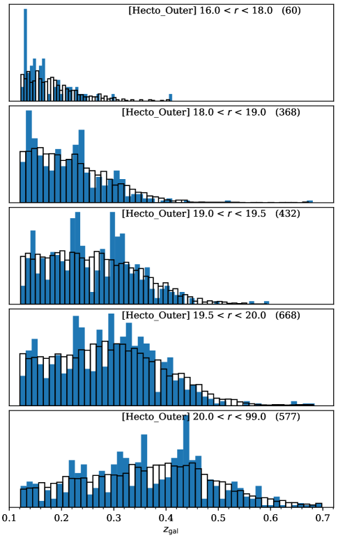
Figure 18: Blue, filled histograms show the redshift distribution for galaxies observed in the outer layer of the Hectospec dataset ($\theta>10^{\prime}$), split by $r$-band magnitude. The number in parenthesis lists the total in each interval. Overlaid in the open, black histogram is a normalized, random distribution drawn from a Cubic-spline fit to a Gaussian-smoothed version of the real histogram. This smooths out the small-scale clustering of the galaxies while maintaining the overall distribution.

For each real galaxy, a set of $n_{\rm rand}=100$ galaxies were placed at its RA/DEC with redshifts drawn randomly from the appropriate sensitivity function. Figure 19 compares the distribution of comoving separations of the real and random galaxies for the sightlines. The close correspondence is vital to the analysis. For each field, we then evaluated the number of data-data ($D_{g}D_{g}$) data-random ($D_{g}R_{g}$) and random-random ($R_{g}R_{g}$) galaxy-galaxy pairs in bins of $0.339h_{100}^{-1}\,{\rm Mpc}$ in the radial ($R_{\parallel}$, line-of-sight) and tangential ($R_{\perp}$, plane-of-sky) directions. We then sum all of the fields and use the L-S estimator:

$$\xi_{\rm gg}(r)^{LS}=\frac{D_{g}D_{g}/n_{gg}^{DD}-2D_{g}R_{g}/n_{gg}^{DR}}{R_{g}R_{g}/n_{gg}^{RR}}+1$$ (1)

to evaluate $\xi_{\rm gg}(r)$ with $n_{gg}^{DD}$, $n_{gg}^{DR}$, and $n_{gg}^{RR}$, the normalization factors. Figure 20 shows the binned evaluation.

Uncertainties in $\xi_{\rm gg}(r)$ have been estimated from the analytic approximation of the variance presented by Landy & Szalay (1993) as (in our notation),

$$\sigma^{2}_{\xi_{gg}}(r)^{LS}\approx\frac{(1+\xi_{gg}^{LS})^{2}}{n_{gg}^{DD}(R_{g}R_{g}/n_{gg}^{RR})}\approx\frac{(1+\xi_{gg}^{LS})^{3}}{D_{g}D_{g}}\;\;.$$ (2)

As typical of such analysis, one observes an asymmetry due to peculiar motions in converting redshift into distance along the line-of-sight (i.e., redshift distortions). Examining the measurements in the transverse separation $R_{\perp}$, one also identifies significant $\xi_{\rm gg}(r)$ signal at large separations which we now quantify.

Figure 19: Normalized histograms comparing the distribution of projected separations from the quasar sightline for the real galaxy sample (DD; black) and the constructed set of random galaxies (RR; red). The close agreement is critical to an unbiased estimate of $\xi_{\rm gg}(r)$.

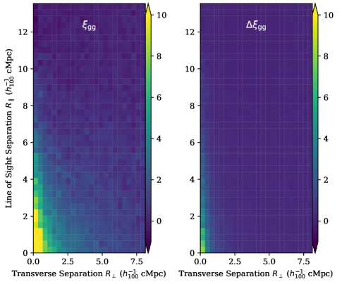
Figure 20: (left) Binned evaluations of the galaxy-galaxy auto-correlation function $\xi_{\rm gg}(r)$ measured from $z<0.75$ galaxies in the CASBaH survey ($0.359\,h_{100}^{-1}\,{\rm Mpc}$ grid). (right) Estimates of the uncertainty in $\xi_{\rm gg}(r)$ derived from the variance of the Landy-Szalay estimator (Equation 2).

To reduce the effects of redshift distortion and also to parameterize the $\xi_{\rm gg}(r)$ measurements, we have evaluated the mean transverse correlation function by averaging $\xi_{\rm gg}(r)$ along the line-of-sight to $R_{\parallel}=13.55\,h_{100}^{-1}\,{\rm Mpc}$,

$$<\xi^{\rm T}_{\rm gg}(R_{\perp})>=\frac{1}{N}\sum\limits_{i}^{N}\xi_{\rm gg}^{i}(r=R_{\perp})\;\;\;,$$ (3)

where the sum is over the 40 bins of $0.339\,h_{100}^{-1}\,{\rm Mpc}$ in the line-of-sight dimension. This quantity is presented in Figure 21, with uncertainties derived from the L-S estimator (see equation 2) for the collapsed pair-counts. Overlaid on the data is the best-fit power-law model for the 3D correlation function $\xi_{\rm gg}(r)=(r/r_{0})^{-\gamma}$ estimated from standard maximum likelihood techniques assuming a Gaussian deviate. The best-fit values are $r_{0}=5.48\pm 0.07\,h_{100}^{-1}\,{\rm Mpc}\,h_{100}^{-1}\,{\rm Mpc}$ and $\gamma=1.33\pm 0.04$ with uncertainties referring to 68% confidence intervals. Specifically, we averaged $\xi_{\rm gg}(r)$ over $R_{\parallel}=[0,13.55]h_{100}^{-1}\,{\rm Mpc}$ at the center of each $<\xi^{\rm T}_{\rm gg}(R_{\perp})>$ bin and constructed the resultant likelihood function by varying $\gamma$ and $r_{0}$. The likelihood evaluation is limited to the transverse bins in the interval $R_{\perp,c}=[1-10]\,h_{100}^{-1}\,{\rm Mpc}$ to isolate the so-called two-halo term of large-scale galaxy-galaxy clustering. The best-fit correlation length is typical of star-forming galaxies at $z\sim 0.3$ (Coil et al., 2017), which is consistent with the properties of our sample (Figure 12, Burchett et al., 2019) We also note that the reported uncertainties are likely underestimated because we have not included all sources of variance, e.g., field-to-field variations (Tejos et al., 2014).

The dashed-line in Figure 21 is an extrapolation of the $<\xi^{\rm T}_{\rm gg}(R_{\perp})>$ evaluation to $R_{\perp,c}<1\,h_{100}^{-1}\,{\rm Mpc}$. At these separations, the measurements well exceed the model which is generally interpreted as galaxy-galaxy clustering within individual halos, aka. the one-halo term. We have also examined $<\xi^{\rm T}_{\rm gg}(R_{\perp})>$ for sub-samples of the full galaxy dataset. Splitting the sample into two redshift bins at $z_{\rm gal}=0.45$, we estimate $<\xi^{\rm T}_{\rm gg}(R_{\perp})>$ values that are approximately 2 times higher for the higher redshift galaxies. This follows from the fact that they are intrinsically more luminous and have higher average stellar mass. Furthermore, the high-$z$ set includes many LRGs from SDSS which have a very high clustering amplitude (e.g., Nuza et al., 2013).

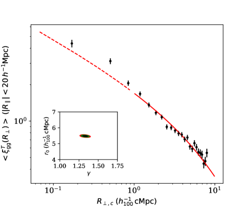
Figure 21: Evaluations of the galaxy-galaxy correlation function averaged along the line-of-sight to $R_{\parallel}=13.55\,h_{100}^{-1}\,{\rm Mpc}$, $<\xi^{\rm T}_{\rm gg}(R_{\perp})>$, in bins of transverse separation. The solid red curve shows the evaluation of $<\xi^{\rm T}_{\rm gg}(R_{\perp})>$ for the best-fit 3D power-law for $\xi_{\rm gg}(r)$ to the data over $R_{\perp,c}=[1-10]\,h_{100}^{-1}\,{\rm Mpc}$. The dashed curve is an extrapolation of this model to $R_{\perp,c}<1\,h_{100}^{-1}\,{\rm Mpc}$ where one notes the data significantly exceed the evaluation. This offset is attributed to galaxy-galaxy clustering within dark matter halos, i.e., the one-halo term. The inset shows the confidence contours from a maximum likelihood analysis which yields $r_{0}=5.48\pm 0.07\,h_{100}^{-1}\,{\rm Mpc}\,h_{100}^{-1}\,{\rm Mpc}$ and $\gamma=1.33\pm 0.04$ at 68% c.l.

6.3 O VI-galaxy Clustering

Inherent to an absorber-galaxy cross-correlation analysis is the notion that absorption systems are measured to occur more (or less) frequently in the proximity of a galaxy than at random. For absorption systems, one can assess the random incidence by surveying many sightlines to estimate the average number per redshift interval, $\ell_{\rm OVI}(z)dz$. Blind surveys for O VI systems along low-$z$ sightlines have yielded direct estimates of $\ell_{\rm OVI}(z)$. Tripp et al. (2008) report $\ell_{\rm OVI}(z)=15.6_{-2.4}^{+2.9}$ at $z=[0.1,0.5]$ from a sample of 51 systems along 16 sightlines for an equivalent width limit of 30 mÅ (i.e., about $\log{N({\rm OVI})}\simeq 13.3$). Danforth et al. (2016) have extended the analysis to 82 sightlines at $z_{\rm QSO}<0.85$ and we estimate $\ell_{\rm OVI}(z)\approx 17$ for ${N({\rm OVI})}>{N({\rm OVI})}_{\rm lim}=10^{13.5}\,{\rm cm^{-2}}$ from their reported statistics (their Table 5; redshift path $\Delta z_{\rm O\,VI}\approx 14.5$). One of the future goals of the CASBaH survey is to measure $\ell_{\rm OVI}(z)$ from our sightlines to $z\sim 1$ (Tripp et al., 2019). As a first estimate, we report 59 systems with ${N({\rm OVI})}>{N({\rm OVI})}_{\rm lim}$ over 7 sightlines giving a redshift path of $\Delta z\approx 7(0.75-0.12)\simeq 4.4$. Therefore, we estimate $\ell_{\rm OVI}(z)\approx 13.5$, consistent with the previous literature (this preliminary estimate is lower because our redshift path is overestimated as it does not take into account parts of the spectra that can be blocked to the O VI absorption). In the following, we adopt $\ell_{\rm OVI}(z)=13.5$ at $z=0.2$ and assume that $\ell(X)$ is constant throughout our analysis window.

Before assessing the O VI-galaxy cross-correlation function $\xi_{\rm ag}(r)$, we begin with an estimate of the covering fraction $f_{C}$ of O VI gas around $z<1$ galaxies. To associate O VI with an individual galaxy, one must adopt a redshift (or velocity) window. Previous work on the CGM has found that the majority of associated gas occurs within a few hundred ${\rm\;km\;s^{-1}}$ of the galaxy redshift (e.g., Prochaska et al., 2011b; Werk et al., 2013). This also holds for CASBaH (Burchett et al., 2018). In the following, we adopt a window of $\delta v=\pm 400{\rm\;km\;s^{-1}}$. We further note that this window is small enough that a chance association with O VI is relatively low. Taking $\ell_{\rm OVI}(z)$ from above, this implies an average of $\mathcal{N}_{\rm OVI}=\ell(z)\delta z\approx 0.03$ systems for $\delta z=(\delta v/c)/(1+z)$.

In a series of arbitrary bins of physical impact parameter $R_{\perp,p}$, we have assessed the fraction of CASBaH galaxies with one or more O VI systems occurring within $\pm 400{\rm\;km\;s^{-1}}$. Any number of galaxies may be associated with a given O VI system. Figure 22 shows the incidence (or covering fraction, $f_{C}$) with uncertainties derived from binomial counting statistics. At small impact parameters ($R_{\perp,p}<100\,\rm kpc$), the incidence is very high: $f_{C}\approx 75\%$. This excess is generally attributed to gas within galaxy halos, i.e., the CGM (see Burchett et al., 2019, for analysis of the O VI CGM in CASBaH). The covering fraction declines monotonically with $R_{\perp,p}$, as expected, but remains $\approx 2\times$ higher than random expectation at the largest offsets probed by CASBaH ($\approx 8\,\rm pMpc$). This implies significant OVI-galaxy clustering on these scales, which we now assess.

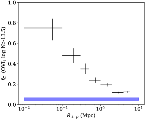
Figure 22: Covering fraction of O VI gas versus physical impact parameter for galaxies in the CASBaH survey to a sensitivity limit of ${N({\rm OVI})}_{\rm lim}=10^{13.5}\,{\rm cm^{-2}}$ with a redshift coincidence within $\pm 400{\rm\;km\;s^{-1}}$. There is a high incidence on small scales that may be attributed to gas within galactic halos (i..e the CGM). At larger impact parameters ($>1$ Mpc), one still recovers $f_{C}$ in excess of random expectation (blue-band), indicating significant O VI-galaxy clustering.

For the cross-correlation analysis of O VI-galaxy clustering, we adopt two approaches. The first follows the analysis developed by Hennawi & Prochaska (2007) to evaluate the clustering of optically thick gas around luminous, $z\sim 2$ quasars (see also, Prochaska et al., 2013). This analysis uses a maximum likelihood approach to estimate the 3D cross-correlation function $\xi_{\rm ag}(r)$ with an assumed functional form of $\xi_{\rm ag}(r)=(r/r_{0})^{-\gamma}$. The likelihood function is given by $\mathcal{L}=(\Pi_{i}P^{\rm hit}_{i})(\Pi_{j}P^{\rm miss}_{j})$ with $P^{\rm hit}$ and $P^{\rm miss}$ the probability of observing one (or more) O VI systems or none, respectively. A galaxy is considered a ‘hit’ if one or more O VI systems occurs within $\pm 400{\rm\;km\;s^{-1}}$ and a miss otherwise, and the likelihood is evaluated from the full dataset satisfying the sample criteria ($\S$ 6.1). The probability of zero absorbers within a velocity window of $\delta v=400{\rm\;km\;s^{-1}}$ is given by Poisson statistics,

$$P^{\rm miss}=\exp\left(\,-[1+\chi_{\perp}]\,\ell_{\rm OVI}(z_{\rm gal})\delta z\,\right)\;\;\;,$$ (4)

where $\ell_{\rm OVI}(z)dz$ is the mean incidence and $\chi_{\perp}$ expresses the boost from clustering i.e., $1+\chi_{\perp}$, with

$$\chi_{\perp}\approx\frac{aH(z)}{2\delta v}\int\limits_{\rm-\delta v/[aH(z)]}^{\rm\delta v/[aH(z)]}dR_{\parallel}\,\xi_{\rm ag}\left(\sqrt{R_{\perp}^{2}+R_{\parallel}^{2}}\right)\;\;\;.$$ (5)

It follows trivially that $P^{\rm hit}=1-P^{\rm miss}$.

We constructed a grid of $\mathcal{L}$ by varying $r_{0}$ and $\gamma$ over a range of values and then found the maximum. Figure 23 presents the constraints on $\gamma$ and $r_{0}$ for the subset of CASBaH galaxies analyzed: galaxies with $R_{\perp,c}=[1,8]\,h_{100}^{-1}\,{\rm Mpc},z=[0.12,0.75]$ and also having no substantial blend at the expected location of O VI. We have estimated the uncertainty by integrating $\mathcal{L}$ down to several confidence limits. The best-fit model is shown on a binned evaluation of $\chi_{\perp}$ in Figure 24. This model provides a good description of the observations at large values and, as with the galaxy-galaxy clustering, we identify a putative one-halo term at $R<0.5h_{100}^{-1}\,{\rm Mpc}$, seen as an excess $\chi_{\perp}$ over the best fit to larger $R_{\perp}$. We note that our results contrast with the O VI-galaxy clustering study by Finn et al. (2016), who find that the O VI-galaxy signal is lower than the galaxy-galaxy autocorrelation on all scales, while here we find similar correlation lengths between them. Still, given the somewhat shallower slope for the O VI-galaxy ($\gamma\approx 1.25$) compared to the galaxy-galaxy one ($\gamma\approx 1.33$), we find that $\xi_{\rm ag}/\xi_{\rm gg}$ should be $\lesssim 1$ on scales $\lesssim 1.3h_{100}^{-1}\,{\rm Mpc}$ (see below). As deeper and more extensive galaxy surveys are completed in the future, it will be valuable to revisit this topic.

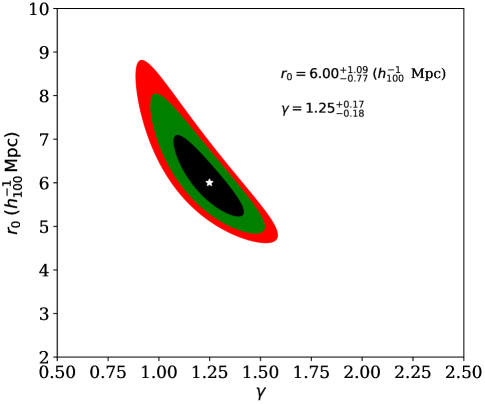
Figure 23: Constraints on $r_{0}$ and $\gamma$ from the O VI-galaxy cross-correlation analysis, resticted to galaxies with $R_{\perp,c}=[1,8]\,h_{100}^{-1}\,{\rm Mpc},z=[0.12,0.75]$ and those without a significant line-blend at O VI.

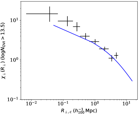
Figure 24: Binned evaluations of $\chi_{\perp}$ derived from the ratio of galaxies with associated O VI absorption relative to random expectation. Overplotted is the evaluation of Equation 5 using the best-fit parameters derived from a maximum likelihood analysis (Figure 23).

We have generated a separate estimate of $\xi_{\rm ag}(r)$ by analyzing the absorber-galaxy pair counts using the formalism applied to $\xi_{\rm gg}(r)$ in $\S$ 6.2. In addition to constructing a set of random galaxies, we must also introduce random absorbers for the absorber-galaxy analysis. These were placed along the sightlines with a uniform redshift distribution in the interval $z=[0.12,0.75]$, avoiding strong Galactic ISM absorption (e.g., Si II 1526) which would preclude the detection of O VI.

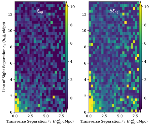
Figure 25: Binned evaluations of $\xi_{\rm ag}(r)$ and its uncertainty as a function of transverse and line-of-sight separation. Similar to the galaxy-galaxy auto-correlation, we observe the effects of redshift distortions and also detect a significant signal to large separations in $R_{\perp}$.

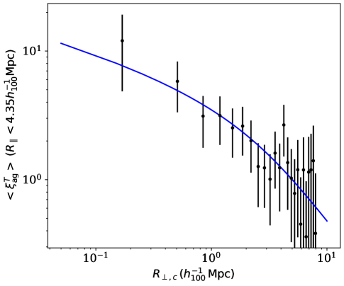
Figure 26: Evaluation of the transverse O VI-galaxy cross-correlation function averaged to $R_{\parallel}=4.4\,h_{100}^{-1}\,{\rm Mpc}$ (corresponding to $\approx 400{\rm\;km\;s^{-1}}$) from the pair analysis. Measurements and uncertainties were derived from the L-S estimator. Overplotted on these values is an evaluation of $<\xi^{\rm T}_{\rm ag}(R_{\perp})>$ using the best-fit model for $\xi_{\rm ag}(r)$ from the $\chi_{\perp}$ analysis.

Figure 25 shows the binned evaluations of $\xi_{\rm ag}(r)$ and its uncertainty. Similar to the galaxy-galaxy auto-correlation, we observe the effects of redshift distortions and also detect a significant signal to large separations in $R_{\perp}$.

To compare with the $\chi_{\perp}$ analysis from above, we calculate $<\xi^{\rm T}_{\rm ag}(R_{\perp})>$ by averaging to $R_{\parallel}=4.4\,h_{100}^{-1}\,{\rm Mpc}$ which corresponds to approximately 400${\rm\;km\;s^{-1}}$ at $z=0.3$. These estimates are shown in Figure 26 and we also overplot the estimate for $<\xi^{\rm T}_{\rm ag}(R_{\perp})>$ based on the best-fit model from Figure 23. There is good overall agreement between the two techniques, although the pair-counting analysis does yield an $\approx 20\%$ lower amplitude at most scales. In the following, we use the pair analysis $\xi_{\rm ag}(r)$ to compare with the auto-correlation function $\xi_{\rm gg}(r)$ but use the power-law fit to $\chi_{\perp}$ for any further discussion of $r_{0},\gamma$.

6.4 Discussion

We now synthesize the results of the previous sub-sections to derive new insight on the physical association of O VI absorption to galaxies. We first remind the reader that the analysis was restricted to O VI systems with ${N({\rm OVI})}\geq 10^{13.5}\,{\rm cm^{-2}}$ and redshift $0.12<z<0.75$. Furthermore, the galaxy sample is dominated by the Hectospec observations and these have $z\sim 0.2-0.4$ and stellar mass of a few $10^{10}M_{\odot}$ (Figure 12).

In the regime of linear bias, we may relate the ratio of the correlation functions to their bias factors,

$$b_{\rm OVI}=b_{gg}\frac{\xi_{ag}}{\xi_{gg}}\;\;,$$ (6)

and further relate the galaxy-galaxy bias $b_{gg}$ to dark matter clustering ($b_{gg}^{2}=\xi_{gg}/\xi_{DM}$) to infer the ‘mean’ halo mass hosting O VI gas. On the latter point, we have made evaluations of $\xi_{DM}$ from the code of Smith et al. (2003) to estimate the galaxy-galaxy bias function at $z=0.3$: $b_{gg}=1.3\pm 0.1$. Following the HOD analysis of Zehavi et al. (2011) for the SDSS main survey ($z\sim 0.1$), we relate $b_{gg}$ to a characteristic halo mass $M_{h}\approx 10^{12.1\pm 0.05}M_{\odot}$.

Figure 27 compares $\xi_{\rm ag}(r)$/$\xi_{\rm gg}(r)$ for the binned evaluations (left) and integrated to $4.4h_{100}^{-1}\,{\rm Mpc}$ and we estimate $\xi_{\rm ag}(r)/\xi_{\rm gg}(r)=0.76\pm 0.1$. This implies that O VI systems are primarily hosted by galaxies in halos with $M_{h}^{\rm OVI}\approx 10^{11}M_{\odot}$, i.e., sub-$L*$ galaxies. These measurements strengthen previous assertions that O VI gas arises primarily in the surroundings of sub-$L*$ galaxies based on CGM statistics (Prochaska et al., 2011b), galaxy-absorber clustering on predominantly smaller scales (Chen & Mulchaey, 2009), and linking individual galaxies to O VI absorbers (Stocke et al., 2006; Pratt et al., 2018). Future work will synthesize these cross-correlation measurements with the statistical incidence of O VI to further assess the physical association of O VI to dark matter halos (e.g., Chen & Tinker, 2008).

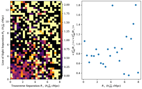
Figure 27: (left) Binned evaluation of the ratio $\xi_{\rm ag}(r)/\xi_{\rm gg}(r)$ which leads to the evaluation of the bias factor for O VI as given by Equation 6. (right) The same ratio averaged along the line-of-sight to $4.4\,h_{100}^{-1}\,{\rm Mpc}$. From these values we estimate $\xi_{\rm ag}(r)/\xi_{\rm gg}(r)=0.76\pm 0.1$.

7 Summary

In this paper we have reviewed the design of a photometric and spectroscopic galaxy redshift survey to support studies of the relationships between QSO absorption-line systems and galaxies, large-scale structures, and other environmental factors. We have reviewed our data handling and measurement methods as well as the content of an on-line public database released with this paper. Combined with absorption-line measurements from high-resolution ultraviolet CASBaH spectroscopy from HST (Tripp et al., 2019), this redshift survey can be used to investigate the role of circumgalactic and intergalactic gases in galaxy evolution, and subsequent papers will exploit the data for various purposes. Importantly, both the galaxies and the absorption systems in the CASBaH database are blindly selected; no explicit preference for galaxies or absorbers of any particular type was imposed on this survey.

As an initial step in our long-term goal of investigating absorber-galaxy-environment connections, we have analyzed the clustering of O VI absorbers with galaxies in the CASBaH database. At small impact parameters, the CASBaH O VI systems with $\log{N({\rm O^{+5}})}>13.5$ and $z<$ 0.75 have high covering fractions that are consistent with earlier studies with different selection criteria (e.g., Prochaska et al., 2011b; Tumlinson et al., 2011; Johnson et al., 2015). This sample also exhibits a covering fraction that is larger than expected from random realizations out to very large projected distances ($\approx$ 8 pMpc), which indicates strong O VI-galaxy clustering, i.e., the gas traces the large-scale structures that comprise the cosmic web.

The clustering of O VI with galaxies is reasonably well described by a power law cross-correlation function of the form $\xi(r)=(r/r_{0})^{-\gamma}$ with $r_{0}$ = $6.00^{+1.09}_{-0.77}\,h_{100}^{-1}\,{\rm Mpc}$ and $\gamma$ = $1.25\pm 0.18$, and the bias implied by our cross-correlation analysis suggests that O VI absorbers are typically affiliated with dark-matter halos having masses $\approx 10^{11}M_{\odot}$ at $z\sim 0.3$.

All of the spectra and photometry derived from our efforts are publicly available in a specDB database file that can be downloaded with that package. The code used to generate the figures and measurements reported here will be released on GitHub with the first set of CASBaH science papers.

References

- Alam et al. (2015) Alam, S., et al. 2015, ApJS, 219, 12, arXiv: 1501.00963
- Aracil et al. (2006) Aracil, B., Tripp, T. M., Bowen, D. V., Prochaska, J. X., Chen, H.-W., & Frye, B. L. 2006, MNRAS, 367, 139
- Bahcall & Peebles (1969) Bahcall, J. N., & Peebles, P. J. E. 1969, ApJ, 156, L7+
- Battisti et al. (2016) Battisti, A. J., Calzetti, D., & Chary, R.-R. 2016, ApJ, 818, 13
- Battisti et al. (2017) —. 2017, ApJ, 851, 90
- Bertin & Arnouts (1996) Bertin, E., & Arnouts, S. 1996, A&AS, 117, 393
- Bertin et al. (2002) Bertin, E., Mellier, Y., Radovich, M., Missonnier, G., Didelon, P., & Morin, B. 2002, in Astronomical Society of the Pacific Conference Series, Vol. 281, Astronomical Data Analysis Software and Systems XI, ed. D. A. Bohlender, D. Durand, & T. H. Handley, 228
- Bielby & et al. (2019) Bielby, R., & et al. 2019, in prep.
- Bond et al. (1996) Bond, J. R., Kofman, L., & Pogosyan, D. 1996, Nature, 380, 603
- Booth et al. (2012) Booth, C. M., Schaye, J., Delgado, J. D., & Dalla Vecchia, C. 2012, MNRAS, 420, 1053
- Bowen et al. (2002) Bowen, D. V., Pettini, M., & Blades, J. C. 2002, ApJ, 580, 169
- Bruzual & Charlot (2003) Bruzual, G., & Charlot, S. 2003, MNRAS, 344, 1000
- Buat et al. (2011) Buat, V., et al. 2011, A&A, 533, A93
- Burchett et al. (2019) Burchett, J., et al., et al., & et al. 2019, in prep.
- Burchett et al. (2018) Burchett, J. N., et al. 2018, arXiv e-prints
- Burchett et al. (2015) —. 2015, ApJ, 815, 91
- Burchett et al. (2013) Burchett, J. N., Tripp, T. M., Werk, J. K., Howk, J. C., Prochaska, J. X., Ford, A. B., & Davé, R. 2013, ApJL, 779, L17
- Calzetti et al. (2000) Calzetti, D., Armus, L., Bohlin, R. C., Kinney, A. L., Koornneef, J., & Storchi-Bergmann, T. 2000, ApJ, 533, 682
- Cantalupo et al. (2014) Cantalupo, S., Arrigoni-Battaia, F., Prochaska, J. X., Hennawi, J. F., & Madau, P. 2014, Nature, 506, 63
- Cautun et al. (2013) Cautun, M., van de Weygaert, R., & Jones, B. J. T. 2013, MNRAS, 429, 1286
- Chabrier (2003) Chabrier, G. 2003, PASP, 115, 763
- Chambers et al. (2016) Chambers, K. C., et al. 2016, ArXiv e-prints
- Chen & Mulchaey (2009) Chen, H., & Mulchaey, J. S. 2009, ApJ, 701, 1219
- Chen et al. (2005) Chen, H.-W., Prochaska, J. X., Weiner, B. J., Mulchaey, J. S., & Williger, G. M. 2005, ApJ, 629, L25
- Chen & Tinker (2008) Chen, H.-W., & Tinker, J. L. 2008, ApJ, 687, 745
- Coil et al. (2017) Coil, A. L., Mendez, A. J., Eisenstein, D. J., & Moustakas, J. 2017, ApJ, 838, 87
- Croft et al. (2002) Croft, R. A. C., Weinberg, D. H., Bolte, M., Burles, S., Hernquist, L., Katz, N., Kirkman, D., & Tytler, D. 2002, ApJ, 581, 20
- Cutri & et al. (2013) Cutri, R. M., & et al. 2013, VizieR Online Data Catalog, 2328
- Dale et al. (2014) Dale, D. A., Helou, G., Magdis, G. E., Armus, L., Díaz-Santos, T., & Shi, Y. 2014, ApJ, 784, 83
- Danforth et al. (2016) Danforth, C. W., et al. 2016, ApJ, 817, 111
- Davis et al. (1985) Davis, M., Efstathiou, G., Frenk, C. S., & White, S. D. M. 1985, ApJ, 292, 371
- Dawson et al. (2013) Dawson, K. S., et al. 2013, AJ, 145, 10
- de Jong et al. (2017) de Jong, J. T. A., et al. 2017, A&A, 604, A134
- Dey et al. (2018) Dey, A., et al. 2018, ArXiv e-prints
- Eisenstein et al. (2001) Eisenstein, D. J., et al. 2001, AJ, 122, 2267
- Faber et al. (2003) Faber, S. M., et al. 2003, in Proceedings of the SPIE, ed. M. Iye & A. F. M. Moorwood, 1657–1669
- Fabricant et al. (2005) Fabricant, D., et al. 2005, PASP, 117, 1411
- Finn et al. (2016) Finn, C. W., et al. 2016, MNRAS, 460, 590
- Flewelling et al. (2016) Flewelling, H. A., et al. 2016, ArXiv e-prints
- Ford et al. (2016) Ford, A. B., et al. 2016, MNRAS, 459, 1745
- Gaia Collaboration et al. (2016a) Gaia Collaboration et al. 2016a, A&A, 595, A2
- Gaia Collaboration et al. (2016b) —. 2016b, A&A, 595, A1
- Ganguly et al. (2013) Ganguly, R., et al. 2013, MNRAS, 435, 1233
- Giallongo et al. (2008) Giallongo, E., et al. 2008, A&A, 482, 349
- Gould & Weinberg (1996) Gould, A., & Weinberg, D. H. 1996, ApJ, 468, 462
- Green et al. (2012) Green, J. C., et al. 2012, ApJ, 744, 60
- Hennawi & Prochaska (2007) Hennawi, J. F., & Prochaska, J. X. 2007, ApJ, 655, 735
- Hewett & Wild (2010) Hewett, P. C., & Wild, V. 2010, MNRAS, 405, 2302
- Howk (2019) Howk, J. C. e. a. 2019, in prep.
- Hudelot et al. (2012) Hudelot, P., et al. 2012, VizieR Online Data Catalog, 2317
- Johnson et al. (2015) Johnson, S. D., Chen, H.-W., & Mulchaey, J. S. 2015, MNRAS, 449, 3263
- Keeney et al. (2018) Keeney, B. A., et al. 2018, ApJS, 237, 11
- Lan & Mo (2018) Lan, T.-W., & Mo, H. 2018, ArXiv e-prints, arXiv:1806.05786
- Landy & Szalay (1993) Landy, S. D., & Szalay, A. S. 1993, ApJ, 412, 64
- Lawrence et al. (2007) Lawrence, A., et al. 2007, MNRAS, 379, 1599
- Lehner et al. (2013) Lehner, N., et al. 2013, ApJ, 770, 138
- Lo Faro et al. (2017) Lo Faro, B., Buat, V., Roehlly, Y., Alvarez-Marquez, J., Burgarella, D., Silva, L., & Efstathiou, A. 2017, MNRAS, 472, 1372
- Lukić et al. (2015) Lukić, Z., Stark, C. W., Nugent, P., White, M., Meiksin, A. A., & Almgren, A. 2015, MNRAS, 446, 3697
- McDowell et al. (1995) McDowell, J. C., Canizares, C., Elvis, M., Lawrence, A., Markoff, S., Mathur, S., & Wilkes, B. J. 1995, ApJ, 450, 585
- Meiring et al. (2013) Meiring, J. D., Tripp, T. M., Werk, J. K., Howk, J. C., Jenkins, E. B., Prochaska, J. X., Lehner, N., & Sembach, K. R. 2013, ApJ, 767, 49
- Miralda-Escudé et al. (1996) Miralda-Escudé, J., Cen, R., Ostriker, J. P., & Rauch, M. 1996, ApJ, 471, 582
- Misawa et al. (2007) Misawa, T., Tytler, D., Iye, M., Kirkman, D., Suzuki, N., Lubin, D., & Kashikawa, N. 2007, AJ, 134, 1634
- Morris et al. (1993) Morris, S. L., Weymann, R. J., Dressler, A., McCarthy, P. J., Smith, B. A., Terrile, R. J., Giovanelli, R., & Irwin, M. 1993, ApJ, 419, 524
- Moustakas et al. (2013) Moustakas, J., et al. 2013, ApJ, 767, 50
- Muzahid et al. (2013) Muzahid, S., Srianand, R., Arav, N., Savage, B. D., & Narayanan, A. 2013, MNRAS, 431, 2885
- Newman et al. (2013) Newman, J. A., et al. 2013, ApJS, 208, 5
- Noll et al. (2009) Noll, S., Burgarella, D., Giovannoli, E., Buat, V., Marcillac, D., & Muñoz-Mateos, J. C. 2009, A&A, 507, 1793
- Nuza et al. (2013) Nuza, S. E., et al. 2013, MNRAS, 432, 743
- Palanque-Delabrouille et al. (2013) Palanque-Delabrouille, N., et al. 2013, A&A, 559, A85
- Pedregosa et al. (2011) Pedregosa, F., et al. 2011, Journal of Machine Learning Research, 12, 2825
- Penton et al. (2002) Penton, S. V., Stocke, J. T., & Shull, J. M. 2002, ApJ, 565, 720
- Pratt et al. (2018) Pratt, C. T., Stocke, J. T., Keeney, B. A., & Danforth, C. W. 2018, ApJ, 855, 18
- Prochaska et al. (2013) Prochaska, J. X., et al. 2013, ApJ, 776, 136
- Prochaska et al. (2011a) Prochaska, J. X., Weiner, B., Chen, H.-W., Cooksey, K. L., & Mulchaey, J. S. 2011a, ApJS, 193, 28
- Prochaska et al. (2011b) Prochaska, J. X., Weiner, B., Chen, H.-W., Mulchaey, J., & Cooksey, K. 2011b, ApJ, 740, 91
- Ribaudo et al. (2011a) Ribaudo, J., Lehner, N., & Howk, J. C. 2011a, ApJ, 736, 42
- Ribaudo et al. (2011b) Ribaudo, J., Lehner, N., Howk, J. C., Werk, J. K., Tripp, T. M., Prochaska, J. X., Meiring, J. D., & Tumlinson, J. 2011b, ApJ, 743, 207
- Rodrigo et al. (2012) Rodrigo, C., Solano, E., & Bayo, A. 2012, The SVO Filter Profile Service
- Sand et al. (2009) Sand, D. J., Olszewski, E. W., Willman, B., Zaritsky, D., Seth, A., Harris, J., Piatek, S., & Saha, A. 2009, ApJ, 704, 898
- Savage et al. (2010) Savage, B. D., et al. 2010, ApJ, 719, 1526
- Schlafly & Finkbeiner (2011) Schlafly, E. F., & Finkbeiner, D. P. 2011, ApJ, 737, 103
- Simcoe et al. (2004) Simcoe, R. A., Sargent, W. L. W., & Rauch, M. 2004, ApJ, 606, 92
- Slosar et al. (2013) Slosar, A., et al. 2013, J. Cosmology Astropart. Phys, 4, 26
- Smith et al. (2003) Smith, R. E., et al. 2003, MNRAS, 341, 1311
- Stocke et al. (2006) Stocke, J. T., Penton, S. V., Danforth, C. W., Shull, J. M., Tumlinson, J., & McLin, K. M. 2006, ApJ, 641, 217
- Tejos et al. (2012) Tejos, N., Morris, S. L., Crighton, N. H. M., Theuns, T., Altay, G., & Finn, C. W. 2012, MNRAS, 425, 245
- Tejos et al. (2014) Tejos, N., et al. 2014, MNRAS, 437, 2017
- Tempel et al. (2014) Tempel, E., Stoica, R. S., Martínez, V. J., Liivamägi, L. J., Castellan, G., & Saar, E. 2014, MNRAS, 438, 3465
- Tripp (2013) Tripp, T. 2013, Science white paper submitted to NASA Solicitation NNH12ZDA008L: Science Objectives and Requirements for the Next NASA UV/Visible Astrophysics Mission Concepts, arXiv:1303.0043
- Tripp et al. (2019) Tripp, T., et al., et al., & et al. 2019, in prep.
- Tripp et al. (1998) Tripp, T. M., Lu, L., & Savage, B. D. 1998, ApJ, 508, 200
- Tripp et al. (2011) Tripp, T. M., et al. 2011, Science, 334, 952
- Tripp et al. (2008) Tripp, T. M., Sembach, K. R., Bowen, D. V., Savage, B. D., Jenkins, E. B., Lehner, N., & Richter, P. 2008, ApJS, 177, 39
- Tumlinson et al. (2011) Tumlinson, J., et al. 2011, Science, 334, 948
- Verner et al. (1994) Verner, D. A., Barthel, P. D., & Tytler, D. 1994, A&AS, 108, 287
- Wakker et al. (2015) Wakker, B. P., Hernandez, A. K., French, D. M., Kim, T.-S., Oppenheimer, B. D., & Savage, B. D. 2015, ApJ, 814, 40
- Wakker & Savage (2009) Wakker, B. P., & Savage, B. D. 2009, ApJS, 182, 378
- Warren et al. (2007) Warren, S. J., et al. 2007, ArXiv Astrophysics e-prints
- Werk et al. (2013) Werk, J. K., Prochaska, J. X., Thom, C., Tumlinson, J., Tripp, T. M., O’Meara, J. M., & Peeples, M. S. 2013, ApJS, 204, 17
- Woodgate et al. (1998) Woodgate, B. E., et al. 1998, PASP, 110, 1183
- Zehavi et al. (2011) Zehavi, I., et al. 2011, ApJ, 736, 59
- Zhu et al. (2014) Zhu, G., et al. 2014, MNRAS, 439, 3139
- Zou et al. (2017a) Zou, H., et al. 2017a, AJ, 153, 276
- Zou et al. (2017b) —. 2017b, PASP, 129, 064101