K-Nearest Neighbor Approximation Via the Friend-of-a-Friend Principle

Abstract.

Suppose $V$ is an $n$-element set where for each $x\in V$, the elements of $V\setminus\{x\}$ are ranked by their similarity to $x$. The $K$-nearest neighbor graph is a directed graph including an arc from each $x$ to the $K$ points of $V\setminus\{x\}$ most similar to $x$. Constructive approximation to this graph using far fewer than $n^{2}$ comparisons is important for the analysis of large high-dimensional data sets. $K$-Nearest Neighbor Descent is a parameter-free heuristic where a sequence of graph approximations is constructed, in which second neighbors in one approximation are proposed as neighbors in the next. Run times in a test case fit an $O(nK^{2}\log{n})$ pattern. This bound is rigorously justified for a similar algorithm, using range queries, when applied to a homogeneous Poisson process in suitable dimension. However the basic algorithm fails to achieve subquadratic complexity on sets whose similarity rankings arise from a “generic” linear order on the $\binom{n}{2}$ inter-point distances in a metric space.

Keywords: similarity search, nearest neighbor, ranking system, linear order, ordinal data, random graph, proximity graph, expander graph
MSC class: Primary: 90C35; Secondary: 06A07

I get by with a little help from my friends.

— John Lennon and Paul McCartney, 1967

1. $K$-Nearest Neighbor Approximation

1.1. Motivation

Approximation to the $K$-nearest neighbor graph for a data set of size $n$ is needed before machine learning algorithms can be applied. Typically $K$ is small (say 5 to 50) but $n$ may be in millions or billions, rendering exhaustive search impractical. Muja and Lowe [25] write: “the most computationally expensive part of many computer vision and machine learning algorithms consists of finding nearest neighbor matches to high dimensional vectors that represent the training data.” Examples include the popular DBSCAN clustering algorithm [12], nearest neighbor classifiers described in Devroye, Györfi & Lugosi [10], and UMAP [24].

1.2. Metric space versus ranking approaches

Metric spaces provide a natural context for similarity rankings. In a finite subset $X$ of a metric space $(\mathcal{X},\rho)$ where for each $x\in X$ the $|X|-1$ distances from $x$ to the other points are distinct, $\rho$ induces a similarity ranking for each point in an obvious way: $x$ is more similar to $y$ than to $z$ iff $\rho(x,y)<\rho(x,z)$. However the $K$-nearest neighbor concept does not require a metric space. It suffices to have an oracle which determines, for distinct points $x,y,z$, whether $y$ is more similar to $x$ than $z$ is. In other words, for each $x$, the oracle knows a ranking of the other points by their similarity to $x$. When two different metrics may be applied to the same set of points, and their induced similarity rankings coincide, any method that proposes two different approximate $K$-nearest neighbor graphs violates common sense, rather like a computation in differential geometry which gives different results in different co-ordinate systems.

Given a finite subset $S$ of $\mathbf{R}^{d}$ with the $L_{p}$ metric, for $1\leq p\leq\infty$, the balanced box-decomposition tree of Arya et al. [2], a variation of the classical k-d tree reviewed in [10], constructs an approximate $K$-nearest neighbor graph in $O(dKn\log{n})$ steps, with a data structure of $O(dn)$ size. Muja and Lowe [25] propose other tree-based algorithms. By using random projections, Indyk & Motwani’s [18] locality sensitive hashing has $O(Kn^{1+\rho}\log{n})$ query time and requires $O(dn+n^{1+\rho})$ space, for a problem-dependent constant $\rho>0$ described in Datar et al. [9], and requires tuning to the specific problem.

Houle and Nett [16] describe a rank-based similarity search algorithm called the rank cover tree, which they claim outperforms in practice both the balanced box-decomposition tree and locality sensitive hashing. Haghiri et al [15] propose another comparison-tree-based nearest neighbor search. Tschopp et al [27] present a randomized rank-based algorithm using the “combinatorial disorder” parameter of Goyal et al [14].

1.3. $K$-nearest neighbor descent

In [11], Dong, Charikar, and Li proposed and implemented a heuristic called $K$-nearest neighbor descent (NND) for approximation to the $K$-nearest neighbor graph. In the metaphor of social networks, their principle is:

(FOF) A friend of a friend could likely become a friend.

We call this the friend-of-a-friend principle (FOF). NND has an appealing simplicity and generality:

• No parameter choices, except $K$.

• No precomputed data structures, such as trees or hash tables.

• Simple, concise code; only the similarity oracle is application-specific.

• No vector embedding is required.

• Randomly initialized – repeated NND runs give alternative approximations.

Perhaps for these reasons, NND was the method of choice in the general-purpose UMAP dimensionality reduction algorithm [4, 24] of McInnes, Healy, et al.

The main drawback of NND has been its lack of any theoretical justification. The present work seeks to shed light on this issue. Various software efficiency optimizations render the algorithm as presented in [11] opaque to rigorous analysis. Instead we analyze non-optimized versions and variations which preserve the essential concept, which is FOF. In [7], we report on observed complexity of a Java Parallel Streams implementation.

1.4. Outline of the paper

We begin by describing NND and several related $K$-nearest neighbor approximation algorithms that take advantage of FOF (Section 2). Next we give examples that show how these algorithms behave in different contexts, succeeding in some and failing in others (Section 4).

We develop the ranking framework in detail, and use it to demonstrate the failure of FOF-based algorithms to achieve sub-quadratic complexity in metric spaces which arise from generic concordant ranking systems (Section 5).

Finally we use random graph methods to prove that one FOF-based algorithm succeeds for a homogeneous Poisson process on a compact metric space with only $O(n\log{n})$ work—better than the $O(n^{1.14})$ claimed in [11] (Section 6).

2. $K$-Nearest Neighbor Approximation Algorithms Exploiting the Friend-of-a-Friend Principle

2.1. Friends and cofriends

Let us first formalize two notions we have used already. For a positive integer $m$, $[m]$ refers to the set $\{1,2,,\ldots,m\}$.

Definition 2.1.

A ranking system $\mathcal{S}=(S,(r_{x})_{x\in S})$ is a finite set $S$ together with, for each $x\in S$, a ranking $r_{x}:S\setminus\{x\}\rightarrow[|S|-1]$ of the other points of $S$. We say that $x$ prefers $y$ to $z$ iff $r_{x}(y)<r_{x}(z)$ (for distinct $x,y,z\in S$). We typically abbreviate $(r_{x})_{x\in S}$ by $\mathbf{r}$.

Definition 2.2.

For a ranking system $\mathcal{S}=(S,\mathbf{r})$ and a positive integer $K<|S|$, the $K$-nearest neighbor graph for $\mathcal{S}$ is the directed graph on $S$ that contains, for each distinct $x,y\in S$, an arc from $x$ to $y$ iff $r_{x}(y)\leq K$.

All the $K$-nearest neighbor approximation algorithms we will describe follow a common framework. They take as input a set $S$ and an integer $K$. In the background is a vector $\mathbf{r}$ of rankings that makes $S$ into a ranking system $\mathcal{S}=(S,\mathbf{r})$. We do not know $\mathbf{r}$ (if we did, we would be done), but we are allowed to query it, in the following sense. For any distinct $x,y,z\in S$, we may ask whether $r_{x}(y)<r_{x}(z)$ or vice-versa. We are never told the value of any $r_{x}(y)$.

The intermediate state of the algorithm is a directed graph on $S$ which represents our current best approximation to the true $K$-nearest neighbor graph for $\mathcal{S}$. Our initial approximation is a uniformly random $K$-out-regular digraph on $S$; that is, each point independently chooses a uniform random set of $K$ initial out-neighbors. In successive iterations called rounds, we allow points to “share information” in some way that, we hope, leverages FOF.

At each round $t$, each point $x$ will be the source of some arcs (usually $K$ of them, except in Section 6.1); we write $F_{t}(x)\subseteq S\setminus\{x\}$ for the set of targets of these arcs, which we call the friends of $x$. The points that view $x$ as a friend are called the cofriends of $x$, denoted

$$C_{t}(x):=\{u\in S\setminus\{x\}:x\in F_{t}(u)\}$$

(possibly $C_{t}(x)=\varnothing$). To leverage FOF, we perform some operation intended to “make introductions” between certain pairs of points which FOF suggests might “get along” (i.e. rank each other highly). As a result of these “introductions,” one (or possibly all, or many) point(s) $x$ updates her friend set if she has just “met” some new point $y$ whom she prefers to some current friend $z$. After these updates, we move to round $t+1$ and repeat. When some condition is met, we stop and return our approximate $K$-nearest neighbor graph.

In a friend list request, a point $x$ asks some other point $y$ to provide $x$ with $F_{t}(y)$, $y$’s current list of friends. Typically $y\in F_{t}(x)$, which leads $x$ to think $y$ might have friends that $x$ would like to meet. Then, via queries to $r_{x}$, $x$ determines her $K$ most-preferred elements of $F_{t}(x)\cup F_{t}(y)\setminus\{x\}$. Finally, $x$ updates her friend set to consist of these $K$ points.

A friend barter is a pair of reciprocal friend list requests, shown in Figure 1. A point $x$ makes a friend list request of another point $y$, and vice-versa, and each updates her respective friend set as appropriate. Typically $y\in F_{t}(x)$, but this does not mean $x\in F_{t}(y)$. Thus $x$ is introduced to friends of a friend, while $y$ is introduced to friends of a cofriend.

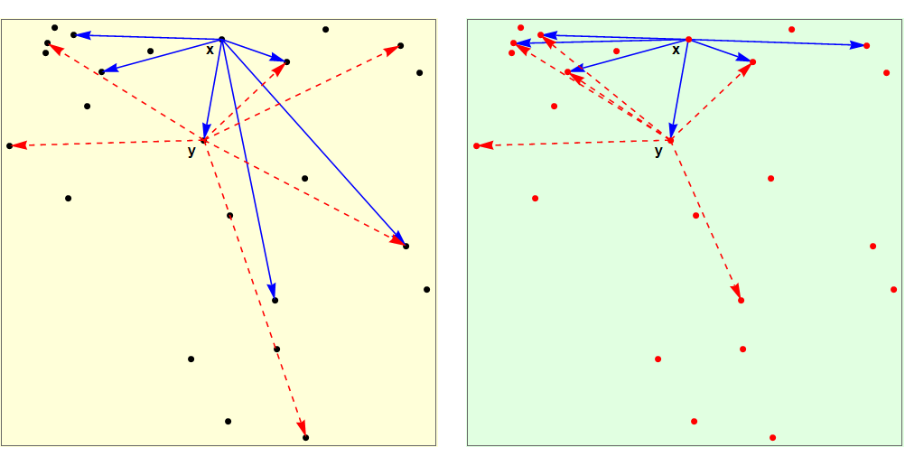
Figure 1. Friend barter: Out of twenty points in the left pane, we show two, each with six friends, indicated by dashed and solid arrows, respectively. Point $y$ is a friend of point $x$. The right pane shows the new friend sets of $x$ and $y$, respectively, after the friend barter. Point $y$ gained three new friends (and discarded three), while point $x$ upper gained two (and discarded two).

Within this framework of iterated “introductions” and updates, specifying an algorithm amounts to deciding which introductions occur in a given round and fixing a stopping condition. Shortly we will specify several algorithms in this way, but before doing so, it is worth reflecting on the initialization step. There is good reason to initialize randomly, quite apart from convenience.

2.2. Consequences of random initialization

Let $D$ be any $K$-out-regular directed graph on $S$, and let $G$ be the corresponding undirected graph, with mean vertex degree about $2K$, obtained by ignoring the direction of arcs in $D$. Consider initializing a FOF-based algorithm with $D$. In any FOF-based algorithm, information travels, via introductions to friends of friends and/or friends of cofriends, by at most 1 step in $G$ per round. Thus if the shortest path in $G$ from $y$ to $x$ has length $d$, any FOF-based algorithm will need to run at least $d-1$ rounds before knowledge of $y$ reaches $x$.

The number of rounds needed for every point to have the possibility of learning about its true nearest neighbors is thus related to the diameter of $G$, i.e. the maximum over $x,y\in S$ of the length of the shortest path from $x$ to $y$. We would like this diameter to be small.

On the other hand, since we initially have no knowledge of $\mathbf{r}$, we should not bias our algorithm by arranging to include, say, an $(n-1)$-leaf star in $G$. Each round involves sorting operations at each point, and to keep these sorts to $O(K^{2}\log K)$ time, the degrees in $G$ need to be kept at $O(K)$.

Taking $D$ uniformly random strikes a good balance. Both the diameter of, and degrees in $G$ are then small. Each point has only a Binomial$(n-1,\frac{K}{n-1})$ number of cofriends. In Lemma A.1 of the Appendix, we will prove that, for $K\geq 3$, with probability tending to 1 as $n\to\infty$, $G$ is an expander graph in the sense of [22], implying that its diameter is $O(\log n)$.

3. Implementations of $K$-nearest Neighbor Descent

3.1. Functional implementation for ranking systems

Darling has published an efficient Java functional implementation of NND, for application to the prank2xy algorithm [8]. The ranking system notion $r_{x}(y)<r_{x}(z)$ is expressed abstractly in terms of a Java Comparator. Batch updates to the $K$-NN approximation are made in parallel using a Collectors method of a Java ParallelStream.

In experiments (see [7, Appendix]) using Kullback-Leibler divergence between points on a $d$-dimensional simplex in $\mathbf{R}^{d}$, our statistical convergence criterion for NND was always satisfied within $\lceil 2\log_{K}{n}\rceil$ batch updates. In these tests, $2\times 10^{4}\leq n\leq 2\times 10^{6}$, $K\in\{16,32,64\}$, and $d\in\{10,20,40,60\}$. Satisfactory approximation was achieved for $K>d$.

We conjecture that $\lceil 2\log_{K}{n}\rceil$ is the correct bound for the number of NND rounds in the ill-defined set of cases where the algorithm works.

3.2. Original implementation for metrics

A sophisticated algorithm for $K$-nearest neighbor descent on points with a symmetric distance function was designed and implemented in [11]. We shall not describe it in detail, except to say that friend sets are not immutable during a round, and the stopping criterion is different to ours. The authors describe in detail the application to five well-studied data sets of sizes between 28,755 and 857,820 using various metrics for similarity.

3.3. Python implementation

McInnes has published the pynndescent Python library. It assumes that similarity is obtained from a metric, of which 22 examples are available in the code. This is one of 19 single-threaded approximate $K$-NN Python algorithms among benchmarks at [5].

3.4. Scheduled pointwise NND

Apply an arbitrary ordering to the $n$ elements of $X$, called the schedule. Initial friend sets $\{F_{0}(x)\}_{x\in X}$ are uniformly random as above. Pass $t$ consists of a set of $n$ friend barters: visit each element of $x\in X$ in the schedule, and update the friends of $x$ by friend barters with all friends of $x$. That means $x$ replaces its former friend set $F_{t-1}(x)$ by a new friend set $F_{t}(x)$, consisting of the $K$ top ranked elements of the set

$$F_{t-1}(x)\cup\left(\bigcup_{y\in F_{t-1}(x)}F_{t-1}(y)\right)\setminus\{x\}.$$

Perform multiple passes until no further changes occur. Note that one pass is not the same as one round of the functional implementation of Section 3.1, in which all friend sets are updated simultaneously by a collect(.) method. This Scheduled pointwise NND was not implemented by us, but is used elsewhere is this paper for theoretical analysis.

4. Examples

This section considers how FOF-based algorithms fare against heterogeneous examples of ranking systems, summarized in Table 1. We mostly restrict attention to ranking systems induced by distance in a metric space $(\mathcal{X},\rho)$, as in Section 1.2. In each such example, the point set of the ranking system will be called $X\subseteq\mathcal{X}$, and $|X|=:n$. For any triples $x,y,z\in X$ with $y\neq z$ but $\rho(x,y)=\rho(x,z)$, we can choose arbitrarily whether $r_{x}(y)<r_{x}(z)$ or vice-versa.

Table 1. Some Contexts for $K$-NND

Point Generation	Metric	FOF Applies?
Leaves of Star Graph	Paris Metric	Yes
Random Points on Circle	Path Metric	Yes
Powers of 2	$\ell_{1}(\mathbf{R})$	Unknown
Random $m$-Strings	Longest Common Subsequence	No ($m$ large)

4.1. Paris metric

Let $\mathcal{X}$ be $\ell_{1}^{n}$, meaning the $n$-dimensional real Banach space where

$$\|(a_{1},\ldots,a_{n})\|=\sum_{1}^{n}|a_{i}|.$$

Let $e_{i}$ denote the $i$-th basis vector. Take $X$ to consist of $n$ points of the form

$$\{x_{i}:=\eta_{i}e_{i}\}_{1\leq i\leq n},$$

where $0<\eta_{1}<\cdots<\eta_{n}$ are real numbers. Then

$$\rho(x_{i},x_{j})=\|x_{i}-x_{j}\|=\eta_{i}+\eta_{j},\quad i\neq j.$$

Project $X$ and an auxiliary point $x_{o}$ into the plane, such that $x_{o}$ maps to the origin, no three points are co-linear, and $x_{i}\in X$ is distance $\eta_{i}$ from $x_{o}$, as in Figure 2; then $\rho$ is called the Paris metric. Using the metropolis as a metaphor, the shortest path between $x_{i}$ and $x_{j}$ is the sum of their distances from the origin. In the graph theory context, view $x_{i}$ as a leaf node of an edge-weighted star centered at $x_{0}\notin X$, where edge $x_{0}x_{i}$ carries weight $\eta_{i}$. The Paris metric is the path metric on this star.

For each $j>K$, the $K$-nearest neighbor set of $x_{j}$ is the set

$$\{x_{1},x_{2},\ldots,x_{K}\}.$$

For $j\leq K$, it is

$$\{x_{1},x_{2},\ldots,x_{K+1}\}\setminus\{x_{j}\}.$$

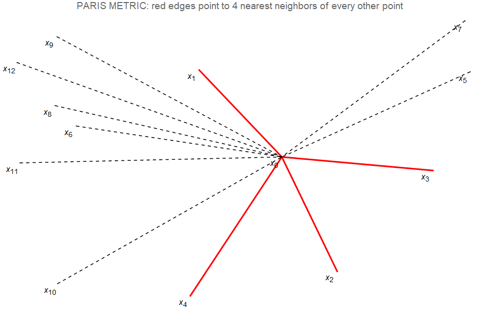
Figure 2. Paris metric: Let $X$ be the leaf nodes of the star graph shown embedded in the plane. The distance between two leaves is the sum of their distances from the central node. Here $K=4$, and 8 of the vertices (dashed arcs) have the same set of $K$ nearest neighbors, which are the $K$ nodes (solid arcs) closest to the center.

NND works well in this example because every pair of vertices are in perfect agreement about how they rank the other $n-2$ vertices. Thus $x_{i}$’s information is always useful—or at least trustworthy—to $x_{j}$, and vice-versa. Each tells the other about the vertices she knows that are closest to $x_{0}$.

Suppose our goal is to discover the $K$-nearest neighbor graph exactly, within some specified number of rounds. Proposition A.1, which bounds the diameter of the initial graph, implies that if $K\geq 3$,

$$r^{*}:=\left\lceil\log_{K-1}(n)\right\rceil$$

rounds of batchwise NND suffice for large $n$, with high probability.

Suppose $i\leq K$, and consider all paths in the initial undirected graph of length $r^{*}$, starting at $x_{i}$ . By Proposition A.1, every point is on one of these paths with high probability. As the algorithm progresses, every other point along each of these paths will retain $x_{i}$ in its friend set. Hence every other point will have $x_{i}$ in its friend set after $r^{*}$ rounds.

4.2. Random points on a circle

Suppose $\mathcal{X}$ is the circle $S^{1}$, and the distance between two points is the angle subtended in radians (i.e. path distance). Let $X$ consist of $n$ points sampled independently according to Lebesgue measure on the circle, or possibly a Poisson$(n)$ number of points. Spatial intuition suggests there may be a constant $\gamma\in(0,1)$, depending on $K$, such that each of the first $T=O(\log{(n/K)})$ rounds of friend set updates multiplies the expected angular span of the friend set of $x$ by $\gamma$ or less. If this is true, then after $T$ rounds of friend set updates, elements of the friend set $F_{T}(x)$ typically lie within a span of $2\pi\gamma^{T}$ radians. The $K$ nearest neighbors of a point typically lie within a span of $2\pi K/n$ radians. If NND works at all in this context, we would expect

$$T:=\lceil(\log{(n/K)})/\log{(1/\gamma)}\rceil$$

rounds to expose these nearest neighbors, after which further friend updates would have no effect. We have been unable to make this argument rigorous for NND, but Section 6 provides a rigorous analysis along these lines for a range-based, rather than a ranking-based, algorithm. The value of $\gamma$ derived in (22) for that algorithm is $\gamma:=1-\sqrt{1-\frac{2}{K}},$ provided $K\geq 3$.

4.3. Random ranking system

In this example there is no metric. Given a set $X$ of size $n$, simply choose a ranking system on $X$ uniformly at random. Do this by choosing for each $x\in X$ a uniformly random ranking $r_{x}$ of $X\setminus\{x\}$, with all choices independent.

There is no hope for decent performance from any FOF-based algorithm in this context, because the FOF principle no longer applies. Since $r_{x},\,r_{y}$ are independent for distinct $x,y$, a point that $y$ ranks highly is no more or less likely to be ranked highly by $x$ than is any other point, regardless of how $x$ and $y$ rank each other.

Consider applying the scheduled pointwise NND of Section 3.4, using only friend list requests. (The analysis would be similar for any other NND variant, if a little less clean.) Consider the progress of the algorithm from the point of view of some fixed $x$. How long until $x$’s friend set contains, say, $\lceil K/2\rceil$ of her true best friends $B:=\{y\in X\setminus\{x\}\;:\;r_{x}(y)\leq K\}$? There is an update at $x$ only every $n$th round, and in these rounds $x$ meets at most $K^{2}$ points, some not for the first time. Each new point $z$ is equally likely to be ranked in any position by $r_{x}$. Thus we expect $x$ to have to meet about $n/2$ points, over the course of at least $n/(2K^{2})$ relevant rounds, before she finds $\lceil K/2\rceil$ points of $B$. Running through $n/(2K^{2})$ relevant rounds means running $n^{2}/(2K^{2})$ rounds total, taking $O(n^{2}\log K)$ work. Essentially, $x$ is performing an inefficient version of exhaustive search during her rounds. Since $x$ was arbitrary, all other points have the same experience.

It is fair to characterize this performance as worse than exhaustive search.

4.4. Longest common substring

Take a finite or countable alphabet $\mathcal{A}$, and a large positive integer $m$. Consider the metric space $(\mathcal{X},\rho)$ consisting of strings $\mathbf{x}:=x_{1}x_{2}\cdots x_{m}$ of length $m$, with characters $x_{i}\in\mathcal{A}$, under the metric based on the longest common substring. To be precise, the length $M(\mathbf{x,x^{\prime}})$ of the longest common substring between two strings is given by

$$M(\mathbf{x,x^{\prime}}):=\max\{s:\exists\,i,j\mbox{ such that }x_{i+1}x_{i+2}\cdots x_{i+s}=x^{\prime}_{j+1}x^{\prime}_{j+2}\cdots x^{\prime}_{j+s}\},$$

and the metric itself is defined by

$$\rho(\mathbf{x,x^{\prime}}):=1-\frac{M(\mathbf{x,x^{\prime}})}{m}.$$

Symmetry $\rho(\mathbf{x,x^{\prime}})=\rho(\mathbf{x^{\prime},x})$ is immediate, as is $\rho(\mathbf{x,x})=0$, while the triangle inequality is verified in a note of Bakkelund [3].

Let $\mu$ be a non-trivial probability measure on $\mathcal{A}$. Let $X\subset\mathcal{X}$ consist of $n$ strings of the form $\mathbf{x}:=X_{1}X_{2}\cdots X_{m}$, where each $X_{i}$ is sampled independently from $\mathcal{A}$ according to the distribution $\mu$, with distinct $\mathbf{x,y}\in X$ independent.

Given three random strings, ties such as $M(\mathbf{x,y})=M(\mathbf{x,z})=q$ will be fairly common. We break ties by ranking $r_{\mathbf{x}}(\mathbf{y})<r_{\mathbf{x}}(\mathbf{z})$ if the product of probabilities of the characters in the longest substring that $\mathbf{y}$ shares with $\mathbf{x}$ is more than the corresponding product for $\mathbf{z}$ and $\mathbf{x}$. If there are still ties, break these arbitrarily.

Given an integer $K$ much smaller than $n$, there is an integer $q_{K}$ (also depending on $m$ and $\mu$) such

$$\Pr[M(\mathbf{x,y})\geq q_{K}+1]<\frac{K}{n}\leq\Pr[M(\mathbf{x,y})\geq q_{K}].$$

The importance of $q_{K}$ is that the $K$ nearest neighbors of $\mathbf{x}$ in $X$ lie within the intersection with $X$ of the ball of radius $1-q_{K}/m$, centered at $x$, which may be written

$$R(\mathbf{x}):=\{\mathbf{y}\in X:M(\mathbf{x,y})\geq q_{K}\}.$$

Arratia, Gordon & Waterman [1, Theorem 2] provide an asymptotic estimate of the value of $q_{K}$ for large $m$. We will not state their theorem precisely, and we omit some intermediate calculations, but the key estimate depends on the sum $p$ of squares of probabilities of characters in the alphabet:

$$p:=\sum_{a\in\mathcal{A}}\mu(\{a\})^{2}\in(0,1).$$

The $K$ nearest neighbors of a specific string $\mathbf{x}$ will typically be strings whose longest common substring with $\mathbf{x}$ has length at least

$$q_{K}=\log_{1/p}(m^{2}(1-p))+\log_{1/p}(n/K)=\frac{2\log(m)+\log((1-p)n/K)}{-\log{p}}.$$

On the other hand, replacing $K$ by 1, the nearest neighbor of $\mathbf{x}$ will typically share a common substring with $\mathbf{x}$ of length $q_{1}$, where

$$q_{1}=\frac{2\log(m)+\log((1-p)n)}{-\log{p}}.$$

Notice that $q_{K}\approx q_{1}\ll m/K$. Thus for any distinct $\mathbf{x,y,z}\in X$, even if $\mathbf{y}$ and $\mathbf{z}$ are ranked highly by $\mathbf{x}$, the longest substring that $\mathbf{x}$ shares with $\mathbf{y}$ will typically be disjoint from that shared between $\mathbf{x}$ and $\mathbf{z}$. In other words, knowing that $\max(r_{\mathbf{x}}(\mathbf{y}),r_{\mathbf{x}}(\mathbf{z}))\leq K$ makes it virtually no more likely that $r_{\mathbf{y}}(\mathbf{z})\leq K$, so $\mathbf{x}$’s information is virtually irrelevant to $\mathbf{y}$ even if $\mathbf{y}$ is a good friend of $\mathbf{x}$, and vice versa, replacing friend by cofriend.

This is precisely the problem we encountered for a random ranking system, if a bit less extreme. The friend of a friend principle is inapplicable for parameters such as the next example.

Numerical example: In “big data” applications, we may have $m$ in the thousands, while $q_{K}$ may be in double digits. For example, if $m=2^{16}$, $n=2^{33}$, $K=2^{5}$, and $p=2^{-4}$, then $q_{K}=15$ and $q_{1}=16$. In other words, the $32$ nearest neighbors of some string $\mathbf{x}$ will typically share common substrings with $\mathbf{x}$ of length $15$ to $17$. Moreover these shared substrings will be different for different neighbors, covering at most a proportion $Kq_{K}/m\approx 2^{-7}$ of the characters in $\mathbf{x}$.

4.5. Powers of 2

Take $\mathcal{X}=\textbf{R}$ with the usual distance, and let $X$ consist of the first $n$ nonnegative powers of 2. For example, the two nearest neighbors of 32 are 16 and 8. We do not know whether NND works here. It seems to lie somewhere between the opposite extremes occupied by the Paris metric of Section 4.1 and the longest common substring metric of Section 4.4. For distinct $x,y$ with $r_{x}(y)\leq K$, there are on average about $K/2$ points $z$ for which $\max(r_{x}(z),r_{y}(z))\leq K$. The corresponding quantity for the Paris metric is $K-1\approx K$; for longest common substring it is $K/n\approx 0$. We revisit the powers of 2 in Example 5.13.

5. Failure of NND

Our goal in this section is to explore what “went wrong” for NND in the longest common substring example. Our intuition is that the rankings $r_{\mathbf{x}}$ and $r_{\mathbf{y}}$ for distinct $\mathbf{x},\mathbf{y}$ are sufficiently “uncorrelated” or “independent” that $\mathbf{y}$’s information is essentially useless to $\mathbf{x}$ even if $\mathbf{y}$ is a friend or cofriend of $\mathbf{x}$. The same problem arose in the case of a random ranking system in Section 4.3. But while it is natural that this would happen for a random ranking system, it is much more surprising in the context of a metric space, because intuitively, the triangle inequality should cause FOF to be helpful.

We now build a framework to formalize these ideas. With this framework in hand, we will prove the striking result that not only is a metric space insufficient to cause FOF to be helpful, but in fact in “almost all” metric spaces FOF fails to help.

5.1. Metrizability and concordancy

Our first step is to nail down just which ranking systems arise from a metric space.

Definition 5.1.

A ranking system $\mathcal{S}=(S,\mathbf{r})$ is called metrizable if there is a metric $\rho$ on $S$ that induces the rankings $\mathbf{r}:=(r_{x})_{x\in S}$, i.e. such that for each distinct $x,y,z\in S$, $\rho(x,y)<\rho(x,z)$ iff $r_{x}(y)<r_{x}(z)$.

Goyal et al. [14] formalize ranking systems in a similar way, but omit the concept of concordancy, which we now define. For a set $X$ and an integer $t$, let $\binom{X}{t}$ denote the set of $t$-element subsets of $X$. As in graph theory we frequently omit brackets for sets of size 2, e.g. $ab:=\{a,b\}$.

Definition 5.2.

Let $\mathcal{S}=(S,\mathbf{r})$ be a ranking system. For $x\in S$, let $\preccurlyeq_{x}$ be the linear order on $S_{x}:=\{xy\;:\;y\in S\setminus\{x\}\}$ (here $xy$ is short for $\{x,y\}$) defined by

$$\{x,r_{x}^{-1}(1)\}\preccurlyeq_{x}\{x,r_{x}^{-1}(2)\}\preccurlyeq_{x}\cdots\preccurlyeq_{x}\{x,r_{x}^{-1}(|S|-1)\}.$$

Formally $\preccurlyeq_{x}$ is a set of ordered pairs of elements of $S_{x}$; for example $\preccurlyeq_{x}$ contains the element $(\{x,r^{-1}_{x}(2)\},\{x,r^{-1}_{x}(5)\})$ (because $2\leq 5$). Let $R_{\mathcal{S}}$ be the union of these sets:

$$R_{\mathcal{S}}\;\;:=\;\;\bigcup_{x\in S}\preccurlyeq_{x}\;;$$

this is a set of ordered pairs of elements of $\cup_{x\in S}S_{x}=\binom{S}{2}$. We call $\mathcal{S}$ concordant if $R_{\mathcal{S}}$ is a subset of some partial order on $\binom{S}{2}$. In this case, the order type of $\mathcal{S}$, denoted $\preccurlyeq_{\mathcal{S}}$, is the unique minimal partial order that contains $R_{\mathcal{S}}$ (i.e. the intersection of all partial orders containing $R_{\mathcal{S}}$).

Henceforth we shorten “concordant ranking system” to CRS.

Example 5.3 (CRS).

Figure 3 shows two views of the ranking system $\mathcal{S}$ on $S=\{a,b,c,d,e\}$ with rankings

$$(1,2,3,4) =(r_{a}(b),r_{a}(e),r_{a}(d),r_{a}(c))$$

$$=(r_{b}(a),r_{b}(c),r_{b}(d),r_{b}(e))$$

$$=(r_{c}(d),r_{c}(e),r_{c}(b),r_{c}(a))$$

$$=(r_{d}(c),r_{d}(e),r_{d}(a),r_{d}(b))$$

$$=(r_{e}(c),r_{e}(a),r_{e}(d),r_{e}(b)).$$

The left of Figure 3 shows, respectively, the linear orders $\preccurlyeq_{a}$ on $S_{a}$; $\preccurlyeq_{b}$ on $S_{b}$; $\preccurlyeq_{c}$ on $S_{c}$; $\preccurlyeq_{d}$ on $S_{d}$; $\preccurlyeq_{e}$ on $S_{e}$. (These are called Hasse diagrams; an arrow appears iff the lower item is less than the upper item and there is no item in between.) Because there exists a partial order on $\binom{S}{2}=\cup_{x\in S}S_{x}$ that simultaneously extends all of these linear orders, $\mathcal{S}$ is concordant. The order type $\preccurlyeq_{\mathcal{S}}$ of $\mathcal{S}$ is the minimal such order, i.e. the one that contains no information beyond what is forced by $R_{\mathcal{S}}$. Its Hasse diagram is on the right of Figure 3.

Figure 3. Concordant ranking system: Example 5.3. The five digraphs on the left show the rankings $r_{a}(\cdot),r_{b}(\cdot),r_{c}(\cdot),r_{d}(\cdot),r_{e}(\cdot)$, respectively. The digraph on the right illustrates the unique minimal partial order extending these rankings to all $\binom{5}{2}$ point pairs.

Example 5.4 (Non-concordant ranking system).

The (unique up to isomorphism) smallest non-concordant ranking system $\mathcal{N}$ has $S=\{a,b,c\}$ and $(1,2)=(r_{a}(b),r_{a}(c))=(r_{b}(c),r_{b}(a))=(r_{c}(a),r_{c}(b))$, and thus $ab\preccurlyeq_{a}ac$, $bc\preccurlyeq_{b}ba$, and $ca\preccurlyeq_{c}cb$. Any relation $R$ containing $R_{\mathcal{N}}$ satisfies $ab\;R\;ac\;R\;bc\;R\;ab$, and thus cannot be both transitive and antisymmetric.

“Almost no” ranking systems are concordant, in the sense that if a set $S$ is made into a ranking system uniformly randomly as in Section 4.3, then the probability that it is concordant tends to 0 as $|S|\rightarrow\infty$; for such a uniformly chosen ranking is expected to contain $\binom{|S|}{3}/4$ triples $\{x,y,z\}\subseteq S$ that are isomorphic to the $\mathcal{N}$ of Example 5.4, and even the lack of such a triple by no means implies concordance.

It turns out that the concordant ranking systems are precisely the metrizable ones.

Lemma 5.5.

For a ranking system $\mathcal{S}=(S,\mathbf{r})$, the following are equivalent:

• $\mathcal{S}$ is concordant;

• $\mathcal{S}$ is metrizable.

Remark: Lemma 5.5 is an easier result than [20, Theorem 4] on ordinal embedding, for which a linear order on all $\binom{n}{2}$ inter-point distances is the input, and a Euclidean embedding is the output.

Proof.

(B) $\Rightarrow$ (A). Suppose $\rho$ is a metric on $S$ inducing $\mathbf{r}$. Since $\mathbf{r}$ has no ties, we are assured that $\rho(x,y)<\rho(x,w)$ if $r_{x}(y)<r_{x}(w)$. Define a binary relation $\preccurlyeq$ on $\binom{S}{2}$ by $xy\preccurlyeq zw$ iff either $xy=zw$ or $\rho(x,y)<\rho(z,w)$ (well-defined by the symmetry of $\rho$).

Evidently this is a partial order since it is reflexive ($xy\preccurlyeq xy$), and inherits antisymmetry and transitivity from the usual order on $[0,\infty)$, the codomain of $\rho$. Now for any $x\in S$, and $y,z\in S\setminus\{x\}$, we have

$$xy\preccurlyeq_{x}xz\quad\Longleftrightarrow\quad r_{x}(y)\leq r_{x}(z)\quad\Longleftrightarrow\quad\rho(x,y)\leq\rho(x,z)\quad\Longleftrightarrow\quad xy\preccurlyeq xz,$$

using the fact that $\rho$ induces $\mathbf{r}$ for the middle equivalence. Thus $\preccurlyeq$ extends each $\preccurlyeq_{x}$, so it extends $R_{\mathcal{S}}$.

(A) $\Rightarrow$ (B). Set $N:=\binom{n}{2}$ and let $\ell^{N}_{\infty}$ denote the $N$-dimensional real Banach space equipped with the sup (max) norm $\|\cdot\|_{\infty}$. Our goal is to exhibit an embedding $f:S\rightarrow\ell^{N}_{\infty}$ satisfying

(1) for each distinct $$x,y,z\in S \|f(x)-f(y)\|_{\infty}<\|f(x)-f(z)\|_{\infty} x y z$$, iff prefers to .

Let $\preccurlyeq$ be any linear order on $\binom{S}{2}$ that extends $\preccurlyeq_{\mathcal{S}}$. Define $\sigma:\binom{S}{2}\rightarrow[N]:=\{1,2,\ldots,N\}$ by

$$\sigma(xy)=\left|\left\{zw\in\tbinom{S}{2}\mid zw\preccurlyeq xy\right\}\right|$$

($\sigma$ enumerates the elements of $\binom{S}{2}$ from “bottom up” according to $\preccurlyeq$). Let $\preccurlyeq^{\prime}$ be an arbitrary linear order on $S$ (needed for technical convenience only). For $x,y,z\in S$ with $y\neq z$ and $y\preccurlyeq^{\prime}z$, set the $\sigma(yz)$th coordinate of $f(x)$ as:

$$f(x)_{\sigma(yz)}=\begin{cases}\;\;\;1+\sigma(yz)/N\quad&\text{if }x=y\\ -1-\sigma(yz)/N\quad&\text{if }x=z\\ \;\;\;0\quad&\text{otherwise.}\end{cases}$$

(To see “what $f$ does,” it may be helpful to read Example 5.6 before continuing.)

We must check (1). Observe that for all $x\in S$ and $zw\in\binom{S}{2}$, each coordinate satisfies $|f(x)_{\sigma(zw)}|\leq 2$. Moreover, for distinct $x,y\in S$, the only coordinate on which $f(x)$ and $f(y)$ are both nonzero is the $\sigma(xy)$th, and

$$|f(x)_{\sigma(xy)}-f(y)_{\sigma(xy)}|=2+2\sigma(xy)/N,$$

which is strictly greater than 2. Thus

$$\|f(x)-f(y)\|_{\infty}=2+2\sigma(xy)/N.$$

This completes the proof: $\preccurlyeq$ extends $\preccurlyeq_{x}$, so $x$ prefers $y$ to $z$ iff $xy\preccurlyeq xz$ iff $\sigma(xy)<\sigma(xz)$ iff $\|f(x)-f(y)\|_{\infty}<\|f(x)-f(z)\|_{\infty}$. ∎

Example 5.6 (Embedding a CRS into $\ell_{\infty}^{N}$).

Let $\mathcal{S}$ be as in Example 5.3, and suppose we want to embed $S$ into $\ell_{\infty}^{10}$ as described in the proof of Lemma 5.5. We first pick a linear extension $\preccurlyeq$ of $\preccurlyeq_{\mathcal{S}}$, say the one shown in the top row of the following table. (The reader can verify by comparing to the Hasse diagram for $\preccurlyeq_{\mathcal{S}}$ that $\preccurlyeq$ is in fact such an extension.) Next we pick an arbitrary linear order $\preccurlyeq^{\prime}$ on $S$, which will determine the signs in the matrix below; say $\preccurlyeq^{\prime}$ orders $S$ alphabetically. Then the function $f$ constructed in the proof of Lemma 5.5 is given in the following table, i.e. the value at row $x$, column $yz$ is $f(x)_{\sigma(yz)}$ (where a blank entry means 0).

$$\begin{array}[]{*{11}r}&ab&\preccurlyeq cd&\preccurlyeq ce&\preccurlyeq ae&\preccurlyeq bc&\preccurlyeq de&\preccurlyeq ad&\preccurlyeq ac&\preccurlyeq bd&\preccurlyeq be\\ a&1.1&&&1.4&&&1.7&1.8&&\\ b&-1.1&&&&1.5&&&&1.9&2\\ c&&1.2&1.3&&-1.5&&&-1.8&&\\ d&&-1.2&&&&1.6&-1.7&&-1.9&\\ e&&&-1.3&-1.4&&-1.6&&&&-2\end{array}$$

Note: each column $xy$ has nonzero entries exactly at rows $x,y$; all column sums are 0; and the absolute value of every nonzero entry is in $(1,2]$. All of this implies that the $\ell_{\infty}$-difference between rows $x$ and $y$ is realized uniquely at column $xy$. This, along with the fact that the absolute values of the nonzero entries increase from left to right (in $\preccurlyeq$ order), implies (1).

5.2. Sampling from the CRSes

We saw in Section 4.3 that FOF-based algorithms fail for generic ranking systems. We aim to show that FOF-based algorithms fail even for generic concordant ranking systems.

Given the concordancy restriction, the word “generic” presents a difficulty. In view of the comment after Example 5.4, a uniformly random ranking system will almost certainly fail to be concordant.

We know of no feasible method to sample uniformly from the CRSes on a set $S$. As there are $(|S|-1)!^{|S|}$ ranking systems, simply listing them and marking the concordant ones is impractical whenever $|S|>6$ (observe $6!^{7}\approx 10^{22}$).

Here is an alternative approach. Given a linear order $\preccurlyeq$ on $\binom{S}{2}$, define, for each distinct $x,y\in S$,

(2) $$r_{x}(y)=\left|\left\{z\in S\setminus\{x\}\;:\;xz\preccurlyeq xy\right\}\right|.$$

Equivalently, define $\preccurlyeq_{x}$ as the restriction of $\preccurlyeq$ to $S_{x}$. This corresponds to reading row $x$ in Example 5.6 and listing the column headings of its nonzero entries left to right.

Evidently the resulting ranking system $(S,(r_{x})_{x\in S})$ is concordant, because there exists a partial order extending $\cup_{x\in S}\preccurlyeq_{x}$, namely $\preccurlyeq$.

Definition 5.7.

If $\preccurlyeq$ is a linear order on $\tbinom{S}{2}$ for some finite set $S$, let $\varphi(\preccurlyeq)$ denote the CRS on $S$ defined by (2):

$$\{$$

Observe that the preimages under $\varphi$ of a CRS $\mathcal{S}$ are precisely the linear extensions of $\preccurlyeq_{\mathcal{S}}$. (This is tautological: by construction $\preccurlyeq$ extends each $\preccurlyeq_{x}$ of $\varphi(\preccurlyeq)$, and by definition $\preccurlyeq_{\varphi(\preccurlyeq)}$ is the minimal partial order that does so, so $\preccurlyeq$ must extend $\preccurlyeq_{\varphi(\preccurlyeq)}$.) Since every partial order has a linear extension, $\varphi$ is surjective. However it is not injective. For example the $\preccurlyeq_{\mathcal{S}}$ of Example 5.3 has many linear extensions, i.e. preimages. We explore this non-injectivity at length in Section 5.5.

Use the term generic CRS on $S$ to refer to the image $\varphi(\preccurlyeq)$ of a uniformly random linear order $\preccurlyeq$ on $\binom{S}{2}$. This corresponds to choosing a metric on $S$ for which the inter-point distances are randomized. Let us reiterate that a generic CRS is far from being a uniformly random CRS.

5.3. NND fails for a generic CRS

As in Section 4.3 we analyze scheduled pointwise version NND of Section 3.4, choosing this variant only for convenience.

Proposition 5.8.

Let $\preccurlyeq$ be a uniformly random linear order on $\binom{S}{2}$. Running scheduled pointwise NND on $\varphi(\preccurlyeq)$, for each $x\in S$ the expected number of rounds needed before $x$’s friend set contains at least $\lceil K/2\rceil$ elements of $B_{x}:=\{y\in X\setminus\{x\}\;:\;r_{x}(y)\leq K\}$ is at least about $n^{2}/(2K^{2})$.

Proposition 5.8 follows easily from the following elementary fact, whose proof we omit.

Lemma 5.9.

Let $\preccurlyeq$ be a uniformly chosen linear order on a finite set $X$, and let $A,B\subseteq X$ be disjoint. Then the random variables $\preccurlyeq|_{A}$ (that is, $\preccurlyeq$ restricted to $A$) and $\preccurlyeq|_{B}$ are independent.

Proof of Proposition 5.8.

Recall $S_{x}:=\{xy:y\in S\setminus\{x\}\}$. Fix $x\in X$, and let $A=\binom{S}{2}\setminus S_{x}$, i.e. point pairs not including $x$. Take

$$\mathcal{S^{\prime}}=(S\setminus\{x\},\mathbf{r^{\prime}})=\varphi(\preccurlyeq|_{A}).$$

Then Lemma 5.9 implies that $r_{x}$, that is $x$’s ranking in $\varphi(\preccurlyeq)$, is independent of $\mathbf{r^{\prime}}$, that is anyone else’s ranking of any third party. In other words, the fact that $y$ is at some time a friend of $x$ does not make $y$’s friend $z$ any better for $x$ than a uniformly selected vertex. The rest of the proof exactly follows Section 4.3: in each of $x$’s friend list requests she discovers at most $K^{2}$ new points, which are from her perspective uniformly random. Thus $x$ expects to have to meet about $n/2$ points, over at least $n/(2K^{2})$ relevant rounds, to find $\lceil K/2\rceil$ points of $B_{x}$. ∎

5.4. CRS perspective on longest common substring

Consider three distinct random strings $\mathbf{x,y,z}$ generated as in Section 4.4. Suppose $\mathbf{a}$, $\mathbf{b}$, and $\mathbf{c}$ are the longest common substrings between $\mathbf{x}$ and $\mathbf{y}$, $\mathbf{y}$ and $\mathbf{z}$, and $\mathbf{z}$ and $\mathbf{x}$ respectively. The lengths of $\mathbf{a,b,c}$ will not exceed $q_{1}\ll m$. Since $\mathbf{a}$ and $\mathbf{b}$ are so short, and likely to occur in different parts of $\mathbf{y}$, their existence does not help to supply a long $\mathbf{c}$. In other words, for $q=1,2,\ldots,q_{1}$

$$\Pr[M(\mathbf{x,z})\geq q\mid\min\{M\mathbf{(x,y}),M(\mathbf{y,z})\}\geq q]\approx\Pr[M(\mathbf{x,z})\geq q].$$

This is essentially the situation when we choose a generic CRS with random inter-point distances, which leads to quadratic run time for NND.

5.5. Digression: properties of the map $\varphi$

Here we begin to explore the many mysteries of the map $\varphi$. We believe this is fertile ground for future research.

Fix a set $S$ of size $n$. Let $L_{n}$ denote the set of $\binom{n}{2}!$ linear orders on $\binom{S}{2}$, and let $R_{n}$ denote the set of CRSes on $S$. Our vantage point for insight into the map (5.7) $\varphi:L_{n}\to R_{n}$ is the following graphical model.

Consider the graph $G$ on vertex set $L_{n}$, taking $\preccurlyeq$ and $\preccurlyeq^{\prime}$ to be adjacent in $G$ iff $\preccurlyeq^{\prime}$ agrees with $\preccurlyeq$ after swapping the order of consecutive items $xy$ and $zw$; here the intersection of $\{x,y\}$ and $\{z,w\}$ could be non-empty. Call $G$ the equivalent metrics graph. Any linear order has $d:=\binom{n}{2}-1$ pairs of consecutive items, so $G$ is $d$-regular. Any linear order can be rearranged into any other via some sequence of swaps of consecutive items, so $G$ is connected.

Color the edges white or black as follows. An edge between $\preccurlyeq$ and $\preccurlyeq^{\prime}$ is colored white if $\varphi(\preccurlyeq)=\varphi(\preccurlyeq^{\prime})$, i.e. if these two linear orders map to the same ranking system, and colored black otherwise.

Proposition 5.10.

An edge of $G$ joining $\preccurlyeq$ and $\preccurlyeq^{\prime}$ is white iff the consecutive items $xy,zw$ that are swapped between $\preccurlyeq$ and $\preccurlyeq^{\prime}$ are disjoint.

Proof.

Simply observe that if $\{x,y\}\cap\{z,w\}=\varnothing$, then for any $u\neq v\in S$, the computation of $r_{u}(v)$ in (2) does not change when $\preccurlyeq$ is replaced by $\preccurlyeq^{\prime}$. If on the other hand $x=w$ (say), then $r_{x}(y)$ and $r_{x}(z)$ swap when $\preccurlyeq$ is replaced by $\preccurlyeq^{\prime}$. ∎

Proposition 5.11.

Let $\preccurlyeq$ and $\preccurlyeq^{\prime}$ be linear orders on $\binom{S}{2}$. Then $\varphi(\preccurlyeq)=\varphi(\preccurlyeq^{\prime})$ iff there is a path of white edges joining $\preccurlyeq$ and $\preccurlyeq^{\prime}$ in $G$.

Proof.

Suppose there is such a path of white edges. Proposition 5.10 implies that all the associated swaps are disjoint, and so $\varphi(\preccurlyeq)=\varphi(\preccurlyeq^{\prime})$. Conversely, suppose $\varphi(\preccurlyeq)=\varphi(\preccurlyeq^{\prime})$. Let $N=\binom{n}{2}$ and consider the “selection sort” algorithm to rearrange the list of pairs $L=(A_{1}\preccurlyeq A_{2}\preccurlyeq\cdots\preccurlyeq A_{N})$ into the list $L^{\prime}=(A^{\prime}_{1}\preccurlyeq^{\prime}A^{\prime}_{2}\preccurlyeq^{\prime}\cdots\preccurlyeq^{\prime}A^{\prime}_{N})$:

• For each $i=1,2,\ldots,N$ do:

  • Find $A^{\prime}_{i}$ in $L$, say at position $j\geq i$

  • Move $A^{\prime}_{i}$ down to position $i$ via $j-i$ swaps involving $A^{\prime}_{i}$ and the item just below.

We claim there are no “bad swaps” (swaps of nondisjoint items). To see this, observe that in the course of the algorithm, for each $i,j$, items $A_{i},A_{j}$ are swapped at most once. Thus if there were a bad swap, say with $A_{i}\cap A_{j}=\{x\}$, then we would have $\varphi(\preccurlyeq)\neq\varphi(\preccurlyeq^{\prime})$ as witnessed by $r_{x}$. ∎

Corollary 5.12.

The subgraph of $G$ consisting of the white edges, which we call the white graph, decomposes into components, each of which consists of the inverse image under $\varphi$ of a distinct CRS.

The components of the white graph vary dramatically in size, from as small as 1 to as large as $(n/2)!^{n-1}\approx\exp(n^{2}\log(n)/2)$ or larger, as the next examples show. To present these examples we adopt the following practical convention. For small $n$, we represent a linear order $\preccurlyeq$ as a matrix where rows are indexed by $S$ and each column is the indicator of an element of $\binom{S}{2}$. We agree that the columns are arranged in $\preccurlyeq$-increasing order left to right (as in Example 5.6), and we leave blanks for zeros.

Example 5.13 (CRS with a unique $\varphi$-preimage).

We return to the powers of 2 example of Section 4.5. Let $S=\{1,2,4,8,16,32\}$ and let $\preccurlyeq$ order the pairs of points of $S$ by their Euclidean distance in $\mathbf{R}$. If row $i$ corresponds to $2^{i}$, and columns are indexed by the vector

$$\setcounter{MaxMatrixCols}{15}\begin{smallmatrix}\{1,2\}&\{2,4\}&\{1,4\}&\{4,8\}&\{2,8\}&\{1,8\}&\{8,16\}&\{4,16\}&\{2,16\}&\{1,16\}&\{16,32\}&\{8,32\}&\{4,32\}&\{2,32\}&\{1,32\}\\ \end{smallmatrix}$$

then $\preccurlyeq$ is represented by the matrix

(9) $$\left[\begin{array}[]{*{15}c}\cdashline{3-3}\cdashline{5-6}\cdashline{8-10}\cdashline{12-15}1&&\lx@intercol\hfil 1\hfil\lx@intercol&&\lx@intercol\hfil\hfil\lx@intercol&\lx@intercol\hfil 1\hfil\lx@intercol&&\lx@intercol\hfil\hfil\lx@intercol&&\lx@intercol\hfil 1\hfil\lx@intercol&&\lx@intercol\hfil\hfil\lx@intercol&&&\lx@intercol\hfil 1\hfil\lx@intercol\\ \cdashline{3-3}1&1&&&\lx@intercol\hfil 1\hfil\lx@intercol&\lx@intercol\hfil\hfil\lx@intercol&&\lx@intercol\hfil\hfil\lx@intercol&1&\lx@intercol\hfil\hfil\lx@intercol&&\lx@intercol\hfil\hfil\lx@intercol&&1&\lx@intercol\hfil\hfil\lx@intercol\\ \cdashline{5-6}&1&1&1&&&&\lx@intercol\hfil 1\hfil\lx@intercol&&\lx@intercol\hfil\hfil\lx@intercol&&\lx@intercol\hfil\hfil\lx@intercol&1&&\lx@intercol\hfil\hfil\lx@intercol\\ \cdashline{8-10}&&&1&1&1&1&&&&&\lx@intercol\hfil 1\hfil\lx@intercol&&&\lx@intercol\hfil\hfil\lx@intercol\\ \cdashline{12-15}&&&&&&1&1&1&1&1&&&&\\ &&&&&&&&&&1&1&1&1&1\\ \end{array}\right].$$

In view of Proposition 5.10, since every pair of consecutive columns shares a nonzero row, every edge of $G$ incident to $\preccurlyeq$ is black. Thus $\preccurlyeq$ is an isolated point of the white graph.

By examining the matrix (9) we can derive a lower bound on the number of isolated points of the white graph. Indeed, if we replace each dashed box in (9) by any permutation matrix of the same size, the resulting matrix represents another isolated point. This is because it retains from (9) the property that every pair of consecutive columns shares a nonzero row. Thus the white graph contains at least $\prod_{k=1}^{n-2}k!\approx\exp(n^{2}\log(n)/2)$ isolated points.

For odd $n$, another source of isolated points in the white graph is Eulerian circuits in the complete graph on $S$. Indeed, if $C=(e_{1},e_{2},\ldots,e_{N})$ is any such circuit, with $N:=\binom{n}{2}$, then the linear order $e_{1}\preccurlyeq e_{2}\preccurlyeq\cdots\preccurlyeq e_{N}$ is an isolated point. This is because since $C$ is a walk, by definition $e_{i}\cap e_{i+1}\neq\varnothing$ for each $i$. McKay and Robinson [26] prove an asymptotic formula for the number of Eulerian circuits on $K_{n}$ in which the dominant term is $\exp(n^{2}\log(n)/2)$, roughly matching the number of isolated points arising from powers-of-2-type orders as above.

Example 5.14 (CRS with many $\varphi$-primages).

For even $n$, the set $\binom{S}{2}$ of edges of the complete graph on $S$ may be partitioned into disjoint perfect matchings $(P_{1},\ldots,P_{n-1})$, according to an elementary form of Baranyai’s theorem [29]. Here $|P_{j}|=n/2$ for every $j$.

Let $\preccurlyeq$ be any linear order on $\binom{S}{2}$ satisfying $xy\preccurlyeq zw$ whenever $xy\in P_{i}$, $zw\in P_{j}$, and $i<j$. Then $\varphi(\preccurlyeq)$ has at least $(n/2)!^{n-1}$ $\varphi$-preimages, because each $P_{i}$ can be arbitrarily reordered (relative to $\preccurlyeq$) independently of the others, without changing the image under $\varphi$. The following matrix represents such a linear order $\preccurlyeq$ with $n=6$. Rows correspond to the six elements of $S$, and columns to the $\binom{6}{2}$ edges of the complete graph on $S$.

$$\left[\begin{array}[]{*4{ccc:}ccc}1&&&&&1&&1&&1&&&1&&\\ 1&&&1&&&&&1&&1&&&&1\\ &1&&1&&&1&&&1&&&&1&\\ &1&&&1&&&1&&&&1&&&1\\ &&1&&1&&1&&&&1&&1&&\\ &&1&&&1&&&1&&&1&&1&\end{array}\right]$$

The dashed vertical lines partition the columns into $n-1$ partitions of $S$, each of size $n/2$. The first three columns represent $P_{1}$, the next three $P_{2}$, etc. Notice that in this example even the consecutive columns that cross the boundaries of the partitions share no nonzero rows, meaning that every edge incident to $\preccurlyeq$ in the equivalent metrics graph is white.

We close this section with two easy calculations intended to give some (minimal) sense of the overall structure of the equivalent metrics graph.

Proposition 5.15.

The probability $p$ that an edge of $G$ selected uniformly at random is white is

$$p:=\frac{\binom{n-2}{2}}{\binom{n}{2}-1}=1-\frac{4}{n+1}.$$

Proof.

Pick a uniformly random edge by (a) picking a uniformly random vertex and then (b) picking a uniformly random edge incident to it. At step (b), out of $d$ possible choices of a pair of consecutive elements $xy,zw$, on average $\binom{n-2}{2}$ of these pairs will be disjoint. ∎

Proposition 5.16 (Linear orders per CRS).

Let $H$ count the linear orders on $\binom{S}{2}$ which lie in the preimage under $\varphi:L_{n}\to R_{n}$ of a CRS on $S$ chosen uniformly at random. Then

(10) $$\frac{\binom{n}{2}!}{((n-1)!)^{n}}\;\;<\;\;\mathbf{E}[H]=\frac{|L_{n}|}{|R_{n}|}\;\;<\;\;\frac{\binom{n}{2}!}{\prod_{k=1}^{n-2}k!}.$$

Remark: Applying Stirling’s approximation for the factorials, the lower bound for $\log{\mathbf{E}[H]}$ has leading term $n^{2}(1-\log(2))/2\approx 0.15n^{2}$, whereas the upper bound for the log has leading term $n^{2}\log(n)/2$.

Proof.

The equality in (10) follows from

$$|R_{n}|\mathbf{E}[H]=\sum_{r\in R_{n}}|\varphi^{-1}(r)|=|L_{n}|.$$

For the inequalities, let $\tilde{R}_{n}\supset R_{n}$ denote the set of all ranking systems (possibly non-concordant) on $S$, and let $R^{1}_{n}\subset R_{n}$ denote the concordant $r\in R_{n}$ for which $|\varphi^{-1}(r)|=1$. It was proved above that

$$|R_{n}|>|R^{1}_{n}|\geq\prod_{k=1}^{n-2}k!.$$

It is immediate from the definitions that

$$|R_{n}|<|\tilde{R}_{n}|=((n-1)!)^{n}.$$

Replacing $|R_{n}|$ in (10) by $|R^{1}_{n}|$ and $|\tilde{R}_{n}|$, the bounds follow. ∎

6. Second Neighbor Range Query on a Homogeneous Poisson Process

6.1. Second neighbor range query

We are disappointed to report that our attempts to bound the complexity of pure ranking-based NND implementations described in Section 3 were not successful. Instead we shall analyze another FOF-based algorithm, called second neighbor range query.

Suppose NND were performed on a set $S$ whose elements are distributed uniformly in a compact metric space $(\mathcal{X},\rho)$. Given the index $t$ of the current round, we should be able to predict roughly the distance $r$ from a typical point to its least-preferred friend. The second neighbor range query algorithm (2NRQ) harnesses this intuition. The principle of 2NRQ, made precise in Section 6.3.1, may be summarized as:

Each vertex allows each pair of its neighbors to discover if they are close to each other.

The basic unit of work in 2NRQ is not a friend barter but a range query. A range query is similar to one round of friend set updates, with changes to the steps that determine membership in the new friend set. In a range query, we fix $r>0$ and we retain some but not all proposed arcs $u\to u^{\prime}$ satisfying $\rho(u,u^{\prime})\leq r$, according to a certain acceptance sampling policy. We discard arcs where $\rho(u,u^{\prime})>r$. The out-degree of of a vertex in the friend digraph is no longer exactly $K$; the idea is to choose $r$ so that the expected out-degree is $K$. A single range query is illustrated in Figure 4.

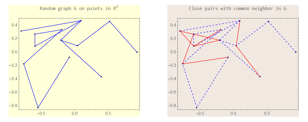
Figure 4. Second neighbor range query: Left: A random graph $G$ with 12 edges among 13 vertices embedded in $[-1,1]^{2}$. Right: The result of a second neighbor range query operation: distinct vertices with a common neighbor in the left graph become adjacent if their separation does not exceed $0.7$. Eight new edges are shown in red. For visual comprehension, edges of $G$ are shown as dashed. Here we gloss over the subtle acceptance sampling of the 2NRQ update discussed in Section 6.3.1.

The 2NRQ algorithm is not proposed for practical use; it is merely the closest algorithm to NND among those whose behavior we can analyze rigorously, at least for the case where the set $S$ is a realization of a homogeneous Poisson process. The only case in which explicit parameters for 2NRQ will be derived is where the metric space is the $d$-dimensional torus with the $\ell_{\infty}$ norm.

Key differences between 2NRQ and NND are:

1. 2NRQ requires a metric space, whereas NND does not.

2. 2NRQ determines friends based on distance, whereas NND queries a ranking oracle.

3. 2NRQ allows vertex degrees to vary, whereas in NND they are fixed at $K$.

4. 2NRQ uses undirected edges, whereas NND uses directed arcs.

5. 2NRQ is a theoretical tool for investigating complexity, whereas NND is proposed for practical deployment.

6.2. Compact metric space with invariant measure

Take a compact metric space $(\mathcal{X},\rho)$, whose topology is second countable and Hausdorff, and which supports a positive finite Borel measure $\lambda$, with the invariance property that all balls of the same radius have the same measure. Without loss of generality, assume that diameter of $\mathcal{X}$ is $\sup\{\rho(x,y):x,y\in\mathcal{X}\}=1$. Denote by $B_{r}(x)$ the closed ball of radius $r$, centered at $x\in\mathcal{X}$, and denote the ratio of the volume of such a ball to the volume of the space by

(11) $$h(r):=\frac{\lambda(B_{r}(x))}{\lambda(\mathcal{X})},\quad x\in\mathcal{X}.$$

Take the finite subset $V\subset\mathcal{X}$ to be the support of a Poisson process with intensity measure $n\lambda(\cdot)/\lambda(\mathcal{X})$, as defined in Kallenberg [19, Ch. 10]. Readers unfamiliar with these terms need only observe that: (1) the size $|V|$ is a Poisson$(n)$ random variable; (2) the number of points of $V$ in any fixed ball of radius $r$ is Poisson$(nh(r))$; and (3) occupancies of disjoint balls are independent.

6.3. 2NRQ graph process

6.3.1. Goal

Our goal is to construct a finite sequence $(V,E_{t})_{0\leq t\leq T}$ of undirected random graphs on $V$, with the aim of presenting $(V,E_{T})$ as an approximate $K$-nearest neighbor graph. In the course of the construction, we will define a sequence of rates $(\theta_{t})$, and a sequence of distances $(r_{t})$:

(12) $$\frac{K}{n}=\theta_{0}<\theta_{1}<\cdots<\theta_{T}<1;\quad 1=r_{0}>r_{1}>\cdots>r_{T}>h^{-1}(K/n),$$

coupled together using the identity

(13) $$\theta_{t}=\frac{K}{nh(r_{t})}.$$

Formulas for $(r_{t})$, and a numerical computation, appear in Sections 6.6.1 and 6.6.2. The graphs $(E_{t})$ will be constructed so as to exhibit a desired sampling property. For every $v\in V$:

The neighbors of $v$ under $E_{t}$ are a random sample at rate $\theta_{t}$ of the elements of

$$Q_{t}(v):=(V\setminus\{v\})\cap B_{r_{t}}(v).$$

In particular, $\rho(v,v^{\prime})>r_{t}$ implies $vv^{\prime}\notin E_{t}$.

This property holds for $t=0$ by construction: $E_{0}$ is obtained by sampling edges of the complete graph on $V$, independently at rate $K/n$.

6.3.2. 2NRQ graph update:

We shall now describe a recursive stochastic construction of $E_{t}$ from $E_{t-1}$, given $r_{t}$, such that the sampling property holds. The idea was presented in Figure 4. A vertex $v^{\prime\prime}$ of degree two or more in $(V,E_{t-1})$ has at least one pair of neighbors. Suppose $(v,v^{\prime})$ is such a pair. If $\rho(v,v^{\prime})>r_{t}$, do nothing. If $\rho(v,v^{\prime})\leq r_{t}$, then edge $vv^{\prime}$ is added to $E_{t}$ according to the success of a Bernoulli$(f_{t}(v,v^{\prime}))$ trial, where the function $f_{t}$ is chosen such that the neighbors of $v$ under $E_{t}$ are distributed uniformly on $Q_{t}(v)$, rather than biased towards points close to $v$. The formula is as follows.

Definition 6.1.

When edge $vv^{\prime}$ is proposed for $E_{t}$, the acceptance sampling rate $f_{t}(v,v^{\prime})$ is zero if $\rho(v,v^{\prime})>r_{t}$, and otherwise is defined as follows. The volume of the intersection of the $r$-balls around $v$ and $v^{\prime}$ is denoted

$$\nu_{r}(v,v^{\prime}):=\lambda(B_{r}(v)\cap B_{r}(v^{\prime}));\quad\rho(v,v^{\prime})\leq r.$$

The minimum value of this volume, over all pairs $v,v^{\prime}$ whose separation does not exceed $s>0$, is

(14) $$g(s,r):=\min_{u,u^{\prime}\in\mathcal{X}:\rho(u,u^{\prime})\leq s}\nu_{r}(u,u^{\prime}).$$

In particular, $g(r_{t},r_{t-1})$ is the volume of intersection of two $r_{t-1}$-balls around points a distance $r_{t}$ apart, which is less than $\nu_{r_{t-1}}(v,v^{\prime})$ when $\rho(v,v^{\prime})<r_{t}$. Take

(15) $$f_{t}(v,v^{\prime}):=\frac{g(r_{t},r_{t-1})}{\nu_{r_{t-1}}(v,v^{\prime})}\leq 1.$$

The function (14) is strictly positive when $0<s<2r$, by the triangle inequality; We shall compute it explicitly for the torus in (18).

The purpose of this acceptance sampling computation will be apparent in the proof of Proposition 6.3: whenever $\rho(v,v^{\prime})\leq r_{t}$, the pool of common neighbors $v^{\prime\prime}$ of both $v$ and $v^{\prime}$ in $E_{t-1}$ has a Poisson number of elements whose mean is

(16) $$\frac{n\theta_{t-1}^{2}\nu_{r_{t-1}}(v,v^{\prime})}{\lambda(\mathcal{X})}$$

which depends on the distance between $v$ and $v^{\prime}$; however this mean is reduced by acceptance sampling to

(17) $$f_{t}(v,v^{\prime})\cdot\frac{n\theta_{t-1}^{2}\nu_{r_{t-1}}(v,v^{\prime})}{\lambda(\mathcal{X})}=\frac{n\theta_{t-1}^{2}g(r_{t},r_{t-1})}{\lambda(\mathcal{X})}$$

which is not affected by the actual distance between $v$ and $v^{\prime}$, if $\rho(v,v^{\prime})\leq r_{t}$.

It is this non-dependence on distance which gives $E_{t}$ the desired sampling property. After this update we shall compute $\theta_{t}$ as the mean rate at which elements of $Q_{t}(v)$ occur as neighbors of $v$ under $E_{t}$.

6.3.3. Value extracted from final graph:

Suppose this procedure can be shown to work in such a way that, substituting from (13),

$$\frac{\theta_{t}n\lambda(B_{r_{t}}(v))}{\lambda(\mathcal{X})}=K,\quad t=0,1,\ldots,T.$$

Then for any $v$, the neighbors of $v$ in $E_{T}$, whose expected number is $K$, form a proportion $\theta_{T}$ of all the points of $V$ within distance $r_{T}$. The key insight is:

If $\theta_{T}\approx 1$, the neighbors of $v$ in $E_{T}$ constitute approximate nearest neighbors of $v$ in $(V,\rho)$.

Given $K$ and the measure $\lambda$, a successful algorithm means designing parameters (12) so that $\theta_{T}\approx 1$ and $T$ is $O(\log{n})$, giving $O(n\log{n})$ total work. This we will do for the torus example in Theorem 6.4. If $O(n)$ steps were required, for example, the algorithm would appear to be useless, since $O(n^{2})$ total work would be required.

6.4. Explicit calculations on the $d$-dimensional torus

6.4.1. Metric embedding of $V$

Let $T^{d}$ denote the $d$ dimensional hypercube $[-1,1]^{d}$ in which opposite faces are glued together to give the $d$-dimensional torus. The metric $\rho$ on $T^{d}$ is induced by the $\ell_{\infty}^{d}$ norm:

$$\rho((x_{1},\ldots,x_{d}),(y_{1},\ldots,y_{d})):=\max_{i}\{\min\{|x_{i}-y_{i}|,|x_{i}-y_{i}\pm 2|\}\}.$$

Henceforward arithmetic on $\mathbf{x}:=(x_{1},\ldots,x_{d})$ will be interpreted so that, for each $i$, replacing $x_{i}$ by $x_{i}\pm 2$ makes no difference. The compact metric space $(T^{d},\rho)$ has diameter $1$. A closed ball centered at $\mathbf{x}$ with radius $r$ is denoted $B_{r}(\mathbf{x})\subset T^{d}$. When $r<1$,

$$B_{r}(\mathbf{0}):=[-r,r]^{d}.$$

Let $\lambda$ denote Lebesgue measure on the Borel sets of $T^{d}$, which has total measure $2^{d}$. The volume ratio function (11) becomes

$$h(r):=\frac{(2r)^{d}}{2^{d}}=r^{d},\quad r\leq 1.$$

Our vertex set $V$ will be a random subset of $T^{d}$ given by a realization of a homogeneous Poisson point process associated with the measure $n2^{-d}\lambda$. Thus the cardinality $|V|$ is a Poisson($n$) random variable.

6.4.2. Intersecting balls on the torus

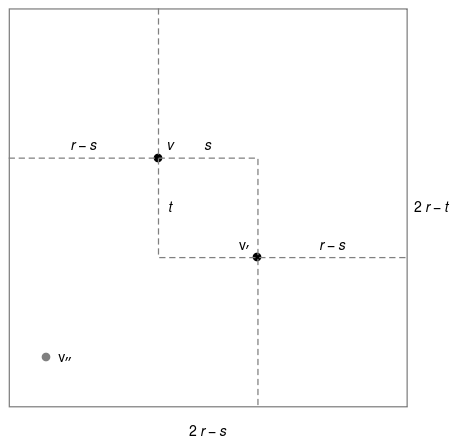
Figure 5. Suppose $0<s<r$, and $v,v^{\prime}$ are two points in $\mathbf{R}^{d}$ with the $\ell_{\infty}^{d}$ norm, separated by distance $s$. The volume of the set of points $v^{\prime\prime}$ within distance $r$ of both $v$ and $v^{\prime}$ is at least $(2r-s)^{d}$. The case $d=2$ is illustrated. Here $0<t\leq s<r$, and $v$ and $v^{\prime}$ differ by $s$ in one coordinate, and $t$ in the other. The locus of points $v^{\prime\prime}$ has area $(2r-s)(2r-t)$, which is at least $(2r-s)^{2}$.

We shall not prove the following geometric fact, but instead ask the reader to inspect Figure 5.

Lemma 6.2.

Consider the metric space $T^{d}$ with the $\ell_{\infty}^{d}$ norm. Suppose $0<s<r<1$. When $\rho(v,v^{\prime})\leq r$, denote by $\nu_{r}(v,v^{\prime})$ the volume of the intersection $B_{r}(v)\cap B_{r}(v^{\prime})$, as in Section 6.3.2. Then

(18) $$g(s,r):=\min_{u,u^{\prime}:\rho(u,u^{\prime})\leq s}\nu_{r}(u,u^{\prime})=\min\{1,(2r-s)^{d}\}.$$

Remark: For another metric, the formula would change. For example, in the Euclidean metric on $\mathbf{R}^{3}$, integral calculus gives

$$\frac{\pi}{12}(4r+s)(2r-s)^{2}.$$

6.5. General update formula for 2NRQ parameters

We shall now establish the validity of the inductive step on which 2NRQ depends, and declare the update formulas for the parameters (12).

Proposition 6.3 (2NRQ parameter update).

Suppose $V$ is a homogeneous Poisson process, with mean cardinality $n$, on a compact metric space $(\mathcal{X},\rho)$ as in Section 6.2. Suppose that, for some $t\geq 1$, and for each $v\in V$. the neighbors of $v$ under $E_{t-1}$ are a uniform random sample at rate $\theta_{t-1}$ of the elements of $V\setminus\{v\}$ in the ball of radius $r_{t-1}$ centered at $v$, where $\theta_{t-1}$ and $r_{t-1}$ are parameters connected by (13). If there exists $r_{t}<r_{t-1}$ satisfying the formula:

(19) $$\left(\frac{K}{nh(r_{t-1})}\right)^{2}\frac{ng(r_{t},r_{t-1})}{\lambda(\mathcal{X})}=-\log\left(1-\frac{K}{nh(r_{t})}\right),$$

use this new radius $r_{t}$ to construct $E_{t}$ according to the 2NRQ update, with acceptance sampling as described in (15). In that case, for each $v\in V$, the neighbors of $v$ under $E_{t}$ are a random sample at rate $\theta_{t}:=K/(nh(r_{t}))$ of the elements of $V\setminus\{v\}$ in the ball of radius $r_{t}$ centered at $v$.

Remark: We do not assert that for every $K,n$, and for every metric space, the equation (19) is solvable for $r_{t}$. See Theorem 6.4.

Proof.

Assume that the random graph $(V,E_{t-1})$ has the properties described. In our probability calculations, we do not condition on any knowledge about the positions of points in $V$ which might have been gathered in previous 2NRQ steps. Let $r_{t}$ be as in (19). Suppose $v,v^{\prime}$ are a pair of vertices with separation $\rho(v,v^{\prime})\leq r_{t}$. By the uniformity hypothesis, the number of vertices

$$v^{\prime\prime}\in B_{r_{t-1}}(v)\cap B_{r_{t-1}}(v^{\prime})$$

is a Poisson random variable with mean

$$\frac{n\nu_{r_{t-1}}(v,v^{\prime})}{\lambda(\mathcal{X})}.$$

Any such vertex $v^{\prime\prime}$ has a probability of

$$\theta_{t-1}^{2}=\left(\frac{K}{nh(r_{t-1})}\right)^{2}$$

of being adjacent to both $v$ and $v^{\prime}$ under $E_{t-1}$. Thus the number of common neighbors of $v$ and $v^{\prime}$ under $E_{t-1}$ is Poisson with the mean given by (16), which is reduced by acceptance sampling to (17), which we shall abbreviate to $\mu$. Note that the formula (17) does not depend on the value of $\rho(v,v^{\prime})$, provided it is less than $r_{t}$. This is the reason why the neighbors of $v$ under $E_{t}$ are uniformly distributed in the ball of radius $r_{t}$ about $v$.

The probability that no edge between $v$ and $v^{\prime}$ exists in $E_{t}$ is $e^{-\mu}$, which is the mass at zero of a Poisson$(\mu)$ random variable. Hence the new rate is

$$\theta_{t}:=\frac{K}{nh(r_{t})}=1-e^{-\mu};\quad\mu=\frac{n\theta_{t-1}^{2}g(r_{t},r_{t-1})}{\lambda(\mathcal{X})}.$$

Rewrite as $\mu=-\log{(1-\theta_{t})}$. After the substitution (13), this is exactly the formula (19).

Thus $E_{t}$ has the desired properties, and the relationship (13) between $\theta_{t}$ and $r_{t}$ has been maintained. ∎

6.6. 2NRQ for uniform points on the torus completes in $O(\log{n})$ steps

Here is our positive result for 2NRQ on the $d$-dimensional torus. We believe that, with more effort, similar results could be obtained for the Euclidean metric on a bounded subset of $\mathbf{R}^{d}$, and for geodesic distance on a sphere.

6.6.1. Formulae for radii:

Parameter computation for 2NRQ amounts to solving (19) for $r_{t}$ in terms of $r_{t-1}$, for as many steps $t$ as desired, to obtain the full parameter sequence (12), where $h(r)=r^{d}$ on the torus. Lemma 6.2 shows that, for the torus, whenever $2r_{t-1}-r_{t}<1$, (19) takes the simpler form

(20) $$\left(\frac{K}{nr_{t-1}^{d}}\right)^{2}\frac{n(2r_{t-1}-r_{t})^{d}}{2^{d}}=-\log\left(1-\frac{K}{nr_{t}^{d}}\right).$$

When $2r_{t-1}-r_{t}\geq 1$, as occurs when $t=1$, (19) specifies $r_{t}$ explicitly in terms of $r_{t-1}$ via the formula

(21) $$-\log\left(1-\frac{K}{nr_{t}^{d}}\right)=\left(\frac{K}{nr_{t-1}^{d}}\right)^{2}\frac{n}{2^{d}}.$$

The proof of Theorem 6.4 shows that there exists $t^{\prime}\geq 1$ such that (21) applies when $t\leq t^{\prime}$, while (20) applies when $t>t^{\prime}$.

6.6.2. An explicit computation of radii for 2NRQ:

For example when $n=10^{7}$, $K=28$, and $d=4$, the criterion $2r_{t-1}-r_{t}\geq 1$ holds only for $t\leq 2$, giving $r_{1}=0.8694$, $r_{2}=0.6572$. For $t\geq 3$, the formula (20) applies. Radii $(r_{t})$ are shown in the following table, together with the corresponding values of $(\theta_{t})$ (when the latter exceed $10^{-4}$):

$t$	0	1	2	3	4	5	6	7	8
$r_{t}$	1.0	0.869	0.657	0.420	0.268	0.171	0.120	0.072	0.052
$\theta_{t}$	-	-	-	-	.0005	.0032	.0191	.1040	.3856

In summary, for $n=10^{7}$, $K=28$, and $d=4$, eight rounds of 2NRQ lead to a graph $(V,E_{8})$ where the neighbors of an arbitrary vertex $v$ constitute about $39\%$ of the elements of $V$ within distance $0.052$ of $v$. No ninth round is shown, because the average vertex degree in $(V,E_{9})$ would drop below $K$.

6.6.3. Parameter estimates:

To prove Theorem 6.4, we shall bound the radii $(r_{t})_{t\geq t^{\prime}}$ between two geometric progressions, which allows us to show that the number of steps of 2NRQ is logarithmic in $n$. For this we prepare some parameter estimates.

The mean number $K$ of neighbors must satisfy a lower bound $K>2^{d}$ in terms of the dimension $d$. This allows us to set the main scaling parameter

(22) $$\gamma:=1-\sqrt{1-\frac{2}{K^{1/d}}}\in(0,1).$$

Indeed since $K>2^{d}$, choose $\beta>1$ such that $K/\beta>2^{d}$, and define $\gamma_{*}\in(\gamma,1)$ via

(23) $$\gamma_{*}:=1-\sqrt{1-2(\beta/K)^{1/d}}\in(0,1).$$

The roles of $\gamma$ and $\gamma_{*}$ will be that $\gamma<r_{t}/r_{t-1}\leq\gamma_{*}$ when $t\geq t^{\prime}$. The proof will mandate that the success rate $\theta_{t}:=K/(nr_{t}^{d})$ does not exceed $\alpha\in(0,1)$, implicitly defined by the formula:

(24) $$\beta:=-\alpha^{-1}\log{(1-\alpha)}.$$

The number $\tau$ of rounds of 2NRQ is a function of the decreasing sequence $(r_{t})$:

(25) $$\tau=\max\{t:r_{t}^{d}\geq\frac{K}{n\alpha}\}.$$

Suppose $\tau>t^{\prime}$, as will happen for large $n$. Since $\gamma<r_{t}/r_{t-1}\leq\gamma_{*}$, the success rates in rounds $t>t^{\prime}$ satisfy:

(26) $$\gamma_{*}^{-d}\leq\frac{\theta_{t}}{\theta_{t-1}}<\gamma^{-d}.$$

It follows that $\alpha\gamma^{d}$ is a lower bound on the success rate, because if $\theta_{t-1}<\alpha\gamma^{d}$, then another round of 2NRQ would still be permissible. Here, for example are parameters corresponding to the numerical example of Section 6.6.2:

$n$	$K$	$d$	$\beta$	$\gamma$	$\gamma_{*}$	$\alpha$	$\tau$	$\alpha\gamma^{d}$
$10^{7}$	28	4	1.386	0.6387	0.7621	0.5	8	0.083

The actual final value of the success rate was $0.3856$, which lies in the interval $(\alpha\gamma^{d},\alpha]$. Doubling the value of $K$ would allow $\beta=2.56$, and a higher success rate of $\alpha=0.9$.

6.6.4. Technical result on 2NRQ

Theorem 6.4 (Homogeneous Poisson process on torus in $d$ dimensions).

Consider a homogeneous Poisson process associated with the measure $n2^{-d}\lambda$ on the $d$-dimensional torus, as described in Section 6.4.1. Assume $K>2^{d}$, choose $\beta\in(1,K/2^{d})$, and set parameters $0<\gamma<\gamma_{*}<1$ and $\alpha$ according to (22), (23) and (24).

1. The update formulas (20) and (21) have a unique solution for $r_{t}$, in terms of $r_{t-1}$, starting at $r_{0}=1$, so long as $r_{t}^{d}\geq K/(n\alpha),$ which allows the 2NRQ algorithm to run for $\tau$ steps as in (25).

2. There is some $t^{\prime}$, depending on $K,\beta$, and $d$, such that the radii $(r_{t})_{t>t^{\prime}}$ are bounded above and below by geometric sequences: $\gamma<r_{t}/r_{t-1}\leq\gamma_{*}.$

3. Suppose $n>K/(\alpha 2^{d})$, which implies $\tau>t^{\prime}$. For each $v\in V$, the neighbors of $v$ under $E_{\tau}$ are a random sample at rate $\alpha\gamma^{d}$ or more of the elements of $V\setminus\{v\}$ in the ball of radius $r_{\tau}$ centered at $v$. The mean number of such neighbors is $K$.

Remark: Corollary 6.5 will use the sub-geometric decay of the radii $(r_{t})$ to prove that, as $n$ increases, $O(\log{n})$ steps of 2NRQ suffice according to (25).

Proof.

On the torus with $\ell_{\infty}^{d}$ norm, we saw that $h(r)=r^{d}$. Lemma 6.2 shows that

$$g(r_{t},r_{t-1})=\min\{1,(2r_{t-1}-r_{t})^{d}\}$$

which implies that distance update formula (19) takes the form (20) or (21) on the torus. To be precise, if $r_{t-1}>1/2$, first try to evaluate $r_{t}$ using (21). If the result satisfies $2r_{t-1}-r_{t}\geq 1$, use this unique value of $r_{t}$. If not, we may assume $r_{t-1}<(1+r_{t})/2$, and so we shall use (20) instead. Since $(r_{t})$ is decreasing, there is some $t^{\prime}\geq 1$, bounded in (28) below, such that the formula (21) applies for $1\leq t\leq t^{\prime}$, and formula (20) applies for $t>t^{\prime}$.

It might happen that $\theta_{t^{\prime}}:=K/(nr_{t^{\prime}}^{d})>\alpha$, in which case we can stop. Otherwise we must check the existence and uniqueness of the solution of (20) for $r_{t}$, in terms of $r_{t-1}<(1+r_{t})/2$, when $t>t^{\prime}$. This will permit application of Proposition 6.3, which will ensure validity of the 2NRQ algorithm. In either case, we shall verify geometric decay of the radii.

Recall that $\beta:=-\alpha^{-1}\log{(1-\alpha)}>1$. Convexity of $x\mapsto-\log{(1-x)}$ guarantees that

$$x<-\log{(1-x)}\leq\beta x,\quad x\in(0,\alpha].$$

It follows that, so long as $t>t^{\prime}$ and $\theta_{t}:=K/(nr_{t}^{d})\leq\alpha$,

(27) $$\frac{K}{nr_{t}^{d}}<-\log\left(1-\frac{K}{nr_{t}^{d}}\right)=\frac{K^{2}}{nr_{t-1}^{d}}\left(1-\frac{r_{t}}{2r_{t-1}}\right)^{d}\leq\frac{\beta K}{nr_{t}^{d}}.$$

Cancel terms in the inequalities, and abbreviate $r_{t}/r_{t-1}<1$ to $y$, to obtain:

$$1<Ky^{d}(1-y/2)^{d}\leq\beta.$$

Divide by $K$, take the $1/d$ power, subtract $1/2$, and complete the square:

$$\frac{1}{K^{1/d}}-\frac{1}{2}<-\frac{1}{2}(1-y)^{2}\leq\left(\frac{\beta}{K}\right)^{1/d}-\frac{1}{2}.$$

Double, change signs, and take the positive square root:

$$\sqrt{1-2(\beta/K)^{1/d}}\leq 1-y<\sqrt{1-2K^{-1/d}}.$$

In other words, there is a unique solution $y:=r_{t}/r_{t-1}<1$ to (19), and this solution satisfies:

$$\gamma<\frac{r_{t}}{r_{t-1}}\leq\gamma_{*},\quad t\geq t^{\prime}.$$

As for the case $1\leq t\leq t^{\prime}$, the pair of inequalities (27) takes the simpler form:

$$\frac{K}{nr_{t}^{d}}<-\log\left(1-\frac{K}{nr_{t}^{d}}\right)=\frac{K^{2}}{n2^{d}r_{t-1}^{2d}}\leq\frac{\beta K}{nr_{t}^{d}}.$$

This shows that the ratios $(r_{t}/r_{t-1})_{1\leq t\leq t^{\prime}}$ satisfy an iteration with the bounds:

$$r_{t-1}\phi<\frac{r_{t}}{r_{t-1}}\leq r_{t-1}\phi_{*},\quad t=1,2,\ldots,t^{\prime};\quad\frac{2}{K^{1/d}}=:\phi<\phi_{*}:=2(\beta/K)^{1/d}<1.$$

An induction, started at $r_{0}=1$, shows that

$$\phi^{2^{t}-1}<r_{t}\leq\phi_{*}^{2^{t}-1},\quad t=1,2,\ldots,t^{\prime}.$$

Since $t\leq t^{\prime}$ can only occur when $r_{t}>1/2$, the number of steps where (21) applies is bounded by a constant determined by $K,\beta$, and $d$:

(28) $$t^{\prime}<\log_{2}{\left(1+1/\log_{2}(1/\phi_{*})\right)}=\log_{2}{\left(\frac{\log_{2}(K/\beta)}{\log_{2}(K/\beta)-d}\right)}.$$

The validity of the bound $\theta_{t}\leq\alpha$ for $t=0,1,2,\ldots,\tau$, is a consequence of the definition (25). Thus Proposition 6.3 applies, and the 2NRQ algorithm runs correctly for $\tau$ steps, at the end of which $\theta_{\tau}\leq\alpha$. If $\theta_{\tau}\leq\alpha\gamma^{d}$, then another round of 2NRQ would be possible, as explained in (26). Thus $\theta_{\tau}>\alpha\gamma^{d}$ provided $\tau>t^{\prime}$, which occurs if $r_{\tau}<1/2$, which in turn follows from $n>K/(\alpha 2^{d})$ by (25). ∎

6.6.5. Work estimates

Corollary 6.5 (2NRQ work estimate for Poisson process on torus in $d$ dimensions).

The mean number of distance evaluations to achieve a success rate at least $\alpha\gamma^{d}$ in the second neighbor range query, with a neighbor average of $K>2^{d}$, is bounded above by a quantity proportional to

$$nK^{2}\left(t^{\prime}+\frac{\log{(n\alpha/K)}}{d\log{(1/\gamma_{*})}}\right)$$

where $t^{\prime}$ does not depend on $n$, provided $-\alpha^{-1}\log{(1-\alpha)}=\beta\in(1,K/2^{d})$. In particular, $O(\log{n})$ rounds of 2NRQ suffice.

Remark: It is not easy to describe how the complexity of 2NRQ varies with dimension, because the quality of the result of the algorithm increases with $\beta$, i.e. with $K/2^{d}$.

Proof.

By Theorem 6.4, part (b), $r_{t}<\gamma_{*}^{t-t^{\prime}}r_{t^{\prime}}$ for $t=t^{\prime}+1,1,\ldots,\tau$. It follows from the definition (25) of $\tau$ that $\gamma_{*}^{d(\tau-t^{\prime})}>\gamma_{*}^{d(\tau-t^{\prime})}r_{t^{\prime}}^{d}>r_{\tau}^{d}\geq K/(n\alpha)$, and thus

$$\tau<t^{\prime}+\frac{\log{(n\alpha/K)}}{d\log{(1/\gamma_{*})}}.$$

At each step, $O(\binom{K}{2})$ neighbor pairs must be checked, for each of $n$ vertices. Hence the upper bound on the work. ∎

7. Conclusions and Future Work

We have seen that NND fails to achieve sub-quadratic complexity for generic concordant ranking systems. It would be interesting to know whether a simiar failure occurs for rank cover trees [16] and comparison trees [15].

The $\lceil\log_{K-1}{n}\rceil$ diameter bound for the expander graph used to initialize NND suggests that $O(\log{n})$ rounds of friend set updates may share enough information for the FOF principle to work. Experiments, reported in a sequel [7], give a class of examples where $2\lceil\log_{K}{n}\rceil$ rounds of friend set updates sufficed for successful convergence of NND provided $K$ exceeded the dimension $d$ in which points were embedded. The second neighbor range query, which exploits FOF but is not based on rankings, provably finishes in $O(\log{n})$ rounds when applied to a class of homogeneous Poisson processes on compact separable metric spaces, but only when $K>2^{d}$ (at least for the $\ell_{\infty}$ norm on the torus).

Combinatorial disorder, introduced by Goyal et al. [14], defines approximate triangle inequalities on ranks. These authors define a disorder constant $D$ such that, in the notation of Definition 2.1,

$$r_{y}(x)\leq D(r_{z}(x)+r_{z}(y)),\quad\forall x,y,z.$$

Possibly some condition on $D$, or a similar notion, would guarantee that NND finishes in $O(n\log{n})$ work with a constant depending on $D$.

Can one say more about the structure of the equivalent metrics graph of Section 5.5? Further insight into its structure may shed light on how frequently NND can be expected to work well in practice. It is possible that our model of a generic CRS is biased in favor of those for which NND has $O(n^{2})$ complexity.

Acknowledgments: The authors thank Leland McInnes (TIMC) for drawing our attention to nearest neighbor descent, and Kenneth Berenhaut and Katherine More (WFU) for valuable discussions about data science based on rankings.

Appendix A Bounding Diameter of the Initial Random Graph

A.1. Main result

To motivate Proposition A.1, observe that the arcs of $D$ refer to the initial friend selections in NND, while edges of $G$ refer to the union of friend and cofriend relations. The diameter of $G$ limits the rate of spread of information in NND.

Proposition A.1.

Suppose $\Gamma_{x}$ is a uniform random $K$-subset of $S\setminus\{x\}$ for each $x\in S$, with $\{\Gamma_{x},x\in S\}$ independent. For $|S|=n$, consider the regular directed graph $D=D^{K}_{n}$ on $S$ with arcs $\bigcup_{x}\{(x,y),y\in\Gamma_{x}\}$, and the corresponding undirected graph $G=G^{K}_{n}$ on $S$ with edges $\bigcup_{x}\{\{x,y\},y\in\Gamma_{x}\}$. Let $B=B_{n}^{K}$ denote the diameter of $G$. For all $K\geq 3$ and $\epsilon>0$,

$$\lim_{n\to\infty}\Pr\left[B_{n}^{K}\leq(1+\epsilon)\log_{K-1}(n)\right]=1.$$

Remark: Bollobás & de la Vega [6] prove that, for any $\epsilon>0$, the diameter of a uniform $K$-regular random graph, with $K\geq 3$, almost surely does not exceed the smallest integer $r$ such that

$$(K-1)^{r}\geq(2+\epsilon)Kn\log{n}.$$

Fernholz & Ramachandran [13, Theorem 5.1] estimate the diameter of graphs generated uniformly at random according to a given vertex degree sequence. When vertex degrees $X_{i}$ are sampled independently with $X_{i}-K\sim$ Binomial$(n-1,\frac{K}{n-1})$, [13, Theorem 5.1] implies a diameter estimate of $\log{(n)}/\log{(2K)}+o(\log{n})$. This does not apply directly to our model, in which vertex degrees are negatively dependent, because they sum to exactly $2Kn$. Krivelevich [22, Lemma 8.2] shows that expander graphs in general have $O(\log{n})$ diameter. We give below a proof from first principles.

A.2. Supporting estimates

Proposition A.1 is an immediate consequence of two estimates concerning $D$. For $X\subseteq S$, let $N(X):=\{y\in S\setminus X\;:\;\exists x\in X\text{ with }y\in\Gamma_{x}\}$.

Proposition A.2 (Vertex Expanders).

With $D$ as in Proposition A.1, for all $\varepsilon>0$, there exists $\alpha>0$ (depending also on $K$) such that the following holds with probability tending to 1 as $n\rightarrow\infty$. For all nonempty $X\subseteq S\text{ with }|X|<\alpha n/\log n$,

(29) $$|N(X)|>(K-1-\varepsilon)|X|.$$

Proof of Proposition A.2.

We follow Vadhan [28, Theorem 4.4] with minor changes. For $l<\alpha n/\log n$ (with $\alpha$ to be defined below), let $p_{l}$ be the probability that there is some $X\subseteq S$ of size exactly $l$ that violates (29). We will show that $\sum_{l=1}^{\alpha n/\log n}p_{l}=o(1)$.

Fix $l$ and $X=\{x_{1},x_{2},\ldots,x_{l}\}\subseteq S$, and imagine choosing one by one the elements of $\Gamma_{x_{1}}$, followed by the elements of $\Gamma_{x_{2}}$, $\ldots$ followed by the elements of $\Gamma_{x_{l}}$. Call a choice bad if the vertex chosen is an element of $X$ or is the same as some previously-chosen vertex. The probability that any particular choice is bad is at most $l(K+1)/n$, even conditioned on all prior choices. Failure of (29) for $X$ requires at least $(1+\varepsilon)l$ bad choices, and thus has probability at most

$$\binom{Kl}{(1+\varepsilon)l}\left(\frac{l(K+1)}{n}\right)^{(1+\varepsilon)l}$$

(the binomial coefficient choosing which choices are bad). Therefore, summing over possible sets $X$ (of size $l$), Stirling’s approximation gives

$$p_{l}\leq\binom{n}{l}\binom{Kl}{(1+\varepsilon)l}\left(\frac{l(K+1)}{n}\right)^{(1+\varepsilon)l} \leq\left(\frac{ne}{l}\right)^{l}\left(\frac{Kle}{(1+\varepsilon)l}\right)^{(1+\varepsilon)l}\left(\frac{l(K+1)}{n}\right)^{(1+\varepsilon)l}$$

$$<\left(\frac{e^{2+\varepsilon}(K+1)^{2+2\varepsilon}}{(1+\varepsilon)^{1+\varepsilon}}\left(\frac{l}{n}\right)^{\varepsilon}\right)^{l}.$$

Now, fix $\alpha=[e^{2+\varepsilon}(K+1)^{2+2\varepsilon}]^{-1/\varepsilon}$ and (for convenience) $\gamma=(1+\varepsilon)^{-(1+\varepsilon)}<1$. Then for all $l<\alpha n/\log n$, we have $p_{l}<\gamma^{l}/(\log n)^{l\varepsilon}\leq\gamma^{l}/(\log n)^{\varepsilon}$, so

$$\sum_{l=1}^{\alpha n/\log n}p_{l}\;<\;(\log n)^{-\varepsilon}\sum_{l=1}^{\infty}\gamma^{l}\;=\;o(1).\qed$$

Let $d_{D}(x,y)$ be the distance from $x$ to $y$ in $D$, and let $N^{r}(x):=\{y\in S\;:\;d_{D}(x,y)=r\}$ and $\overline{N}^{r}(x):=\cup_{i=0}^{r}N^{i}(x)$.

Proposition A.3 (Diameter Bound).

With $D$ as in Lemma A.1 and any $\varepsilon>0$, the following holds with probability tending to 1 as $n\rightarrow\infty$. For all $x,y\in S$, letting $r=\lceil\log_{(K-1-\varepsilon)}(2n\log n)^{1/2}\rceil$, either

(30) $$\overline{N}^{r}(x)\cap\overline{N}^{r}(y)\neq\varnothing$$

or $\exists z\in N^{r}(x),w\in N^{r}(y)$ such that $w\in\Gamma_{z}$; in other words, the diameter of $G$ does not exceed $2r+1$.

Proof of Proposition A.3.

Fixing any $Y\subseteq S$ and $z\in S\setminus Y$,

$$\Pr(\Gamma_{z}\cap Y=\varnothing) =\left(\frac{n-|Y|}{n-1}\right)\cdots\left(\frac{n-|Y|-K+1}{n-K}\right)<\left(\frac{n-|Y|+1}{n}\right)^{K}$$

$$\qquad=\left(1-\frac{|Y|-1}{n}\right)^{K}<\exp[-K(|Y|-1)/n].$$

For any $x,y$, Proposition A.2 implies $|N^{r}(x)|>\sqrt{2n\log n}$, and likewise for $y$. Fix $x,y$, and condition on the event that $\overline{N}^{r}(x)\cap\overline{N}^{r}(y)$ is empty; the conditional probability that there exists no $z\in N^{r}(x),w\in N^{r}(y)$ for which $w\in\Gamma_{z}$ is at most $\exp[-K|N^{r}(x)||N^{r}(y)|/n]<\exp[-2K\log n]=n^{-2K}$. This bound is the same for all $x,y$. Summing over the $n^{2}$ choices of $x,y$ yields a probability at most $n^{2-2K}=o(1)$ of the existence of a particular $x,y$ for which the shortest connecting path exceeds length $2r+1$. ∎

A.3. Proof of Proposition A.1

To complete the proof of Proposition A.1, the distance in $G$ between any $x,y\in S$ satisfying one of the alternatives in Proposition A.3 is at most $2r+1$, with $r$ as in Proposition A.3. Now

$$2r+1<(1+o(1))\frac{\log n}{\log(K-1)+\log(1-\varepsilon)},$$

which we want to show to be at most

$$(1+\epsilon)\frac{\log n}{\log(K-1)},$$

for some fixed $\epsilon$. Since Proposition A.3 holds for any $\varepsilon$, we can easily choose $\varepsilon$ sufficiently small.

References

- [1] Richard Arratia; Louis Gordon; Michael Waterman. An extreme value theory for sequence matching. Annals of Statistics, Volume 14, Number 3 971-993, 1986
- [2] S. Arya; D. M. Mount; N. S. Netanyahu; R. Silverman; A. Y. Wu. An optimal algorithm for approximate nearest neighbor searching fixed dimensions. Journal of the ACM, Volume 45, pages 891–923, 1998
- [3] D Bakkelund. An LCS-based string metric. Unpublished notes, University of Oslo. 2009
- [4] Etienne Becht; Leland McInnes; John Healy; Charles-Antoine Dutertre; Immanuel W. H. Kwok; Lai Guan Ng; Florent Ginhoux; Evan W. Newell. Dimensionality reduction for visualizing single-cell data using UMAP. Nature Biotechnology volume 37, pages 38–-44, 2019
- [5] Erik Bernhardsson. Benchmarks of approximate nearest neighbor libraries in Python. github.com/erikbern/ann-benchmarks
- [6] B. Bollobás; W. F. de la Vega. The diameter of random regular graphs. Combinatorica 2, 125-134, 1982
- [7] R W R Darling. Experiments with comparator-based nearest neighbor descent. In preparation, 2020
- [8] R W R Darling. prank2xy: Clustering and low dimensional projection of ranking systems. github.com/probabilist-us/prank2xy, 2020
- [9] Mayur Datar; Nicole Immorlica; Piotr Indyk; Vahab S. Mirrokni. Locality-sensitive hashing scheme based on p-stable distributions. In Proceedings of the twentieth annual symposium on computational geometry (SCG ’04). ACM, New York, NY, USA, 253-262, 2004
- [10] Luc Devroye; Laszlo Györfi; Gabor Lugosi. A Probabilistic Theory of Pattern Recognition. Springer Science & Business Media, 2013
- [11] Dong, Wei; Charikar, Moses; Li, Kai. Efficient k-nearest neighbor graph construction for generic similarity measures. Proceedings of the 20th International Conference on World Wide Web, 577–586, 2011
- [12] M. Ester; H.-P. Kriegel; J. Sander; X. Xu. A density-based algorithm for discovering clusters in large spatial databases with noise. Proc. 2nd Int. Conf. Knowl. Discov. Data Mining, 226–-231, 1996
- [13] Daniel Fernholz; Vijaya Ramachandran. The diameter of sparse random graphs. Random Structures and Algorithms 31, 482-516, 2007
- [14] N. Goyal; Y. Lifshits; H. Schutze. Disorder inequality: a combinatorial approach to nearest neighbor search. WSDM ’08 Proc. Intern. Conf. Web Search Web Data Mining 25–-32, 2008
- [15] Siavash Haghiri; Debarghya Ghoshdastidar; Ulrike von Luxburg. Comparison based nearest neighbor search. arXiV: 1704.01460, 2017
- [16] Michael E. Houle; Michael Nett. Rank-based similarity search: reducing the dimensional dependence. IEEE Transactions on Pattern Analysis and Machine Intelligence 37, 136-150, 2015
- [17] Mark Huber. Fast perfect sampling from linear extensions. Discrete Mathematics 306. 420 – 428, 2006
- [18] P. Indyk; R. Motwani. Approximate nearest neighbors: towards removing the curse of dimensionality. Thirteenth Symposium on Theory of Computing, pages 604-–613, 1998.
- [19] Olav Kallenberg. Foundations of Modern Probability, 2nd ed. Springer, New York 2001.
- [20] M. Kleindessner; U. von Luxburg. Uniqueness of ordinal embedding. JMLR: Workshop and Conference Proceedings vol 35:1–28, 2014
- [21] M. Kleindessner; U. von Luxburg. Lens depth function and k-relative neighborhood graph: versatile tools for ordinal data analysis. Journal of Machine Learning Research 18, 1-52, 2017
- [22] M. Krivelevich. Expanders: How to find them, and what to find in them. Surveys in Combinatorics, ed. A. Lo, R. Mycroft, G. Perarnau, A. Treglown, Cambridge University Press 2019
- [23] Leland McInnes. pynndescent: A Python nearest neighbor descent for approximate nearest neighbors. github.com/lmcinnes/pynndescent, 2018
- [24] Leland McInnes; John Healy; James Melville. UMAP: uniform manifold approximation and projection for dimension reduction. arXiv:1802.03426, 2018
- [25] Marius Muja; David G. Lowe. Scalable nearest neighbor algorithms for high dimensional data. IEEE Transactions on Pattern Analysis and Machine Intelligence, 36, 2227–2240, 2014
- [26] B. McKay; R. W. Robinson. Asymptotic enumeration of Eulerian circuits in the complete graph. Combinatorica: 10, no. 4, pages 367–-377, 1995
- [27] D. Tschopp; S. Diggavi; P. Delgosha. Randomized Algorithms for Comparison-based Search. NIPS 2011
- [28] Salil P. Vadhan. Pseudorandomness. Foundations and Trends in Theoretical Computer Science: Vol. 7,No. 1–3, pp 1–336, 2012
- [29] J. H. van Lint; R. M. Wilson. A Course in Combinatorics (2nd ed.). Cambridge University Press, 2001