On Object Symmetries and 6D Pose Estimation from Images

Abstract

Objects with symmetries are common in our daily life and in industrial contexts, but are often ignored in the recent literature on 6D pose estimation from images. In this paper, we study in an analytical way the link between the symmetries of a 3D object and its appearance in images. We explain why symmetrical objects can be a challenge when training machine learning algorithms that aim at estimating their 6D pose from images. We propose an efficient and simple solution that relies on the normalization of the pose rotation. Our approach is general and can be used with any 6D pose estimation algorithm. Moreover, our method is also beneficial for objects that are ’almost symmetrical’, i.e. objects for which only a detail breaks the symmetry. We validate our approach within a Faster-RCNN framework on a synthetic dataset made with objects from the T-Less dataset, which exhibit various types of symmetries, as well as real sequences from T-Less.

1 Introduction

3D object detection and pose estimation are of primary importance for tasks such as robotic manipulation, virtual and augmented reality and they have been the focus of intense research in recent years, mostly due to the advent of Deep Learning based approaches and the possibility of using large datasets for training such methods [12, 7, 17, 23, 27, 16, 29, 22].

However, one challenge is often ignored in recent works. Many objects of our daily life or from industrial contexts exhibit symmetries, or at least ’quasi-symmetries’ when only a small detail prevents the object to have a perfect symmetry. These symmetries create ambiguities when aiming to estimate the 6D pose of the object from images, however only a few recent papers have considered the problems raised by object symmetries [23, 26, 2, 19]. In this paper, we first explain why exactly symmetries can be a problem for 6D pose estimation algorithms. We then provide a simple solution that is general and can be introduced in any 6D pose estimation algorithms.

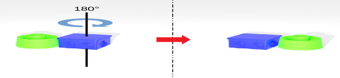
Figure 1: Two views of the same scene before and after a rotation of $180\degree$ around the vertical axis of the blue object. Since this object is symmetrical, it has the same appearance but its pose is different.

To better understand the problem raised by the symmetries of an object, let’s first consider Fig. 1. The blue object has a rotational symmetry around the vertical axis: If we apply a rotation of $180\degree$ around this axis, this object has exactly the same appearance. More generally, when an object $O$ has some symmetry, there exist one or more rigid motions such that, if we apply these rigid motions to the object pose, the appearance of the object is preserved. Formally, we consider the set

$$\mathcal{M}=\{ \boldsymbol{m}\in\text{SE}(3)\text{ such that }$$ (1)

$$\forall\boldsymbol{p}\in\text{SE}(3),\>\>\>\mathcal{R}(O,\boldsymbol{p})=\mathcal{R}(O,\boldsymbol{m}.\boldsymbol{p})\}\>,$$

where $\mathcal{R}(O,\boldsymbol{p})$ is the image of Object $O$ under pose $\boldsymbol{p}$ (ignoring lighting effects), $\boldsymbol{m}$ is a rigid motion related to the symmetry, and $\boldsymbol{m}.\boldsymbol{p}$ is the pose after applying motion $\boldsymbol{m}$. $\mathcal{M}(O)$ is thus the set of rigid motions $\boldsymbol{m}$ that preserve the visual aspect of a given object. It is easy to see that it forms a subgroup of $SE(3)$. [2] calls the elements of $\mathcal{M}(O)$ proper symmetries.

In other words, two images of a symmetrical object can be identical but not correspond to the same pose. If we consider an image $\boldsymbol{I}_{1}=\mathcal{R}(O,\boldsymbol{p})$ of an object $O$ under pose $P$ and a motion $\boldsymbol{m}\in\mathcal{M}(O)$, then, the image $\boldsymbol{I}_{2}$ of object $O$ under pose $\boldsymbol{m}.\boldsymbol{p}$ is equal to image $\boldsymbol{I}_{1}$, i.e. $\boldsymbol{I}_{2}=\mathcal{R}(O,\boldsymbol{m}.\boldsymbol{p})=\mathcal{R}(O,\boldsymbol{p})=\boldsymbol{I}_{1}$. There is therefore no function

$$\mathcal{F}:\boldsymbol{I}\mapsto\boldsymbol{p}$$ (2)

that can provide the pose $\boldsymbol{p}$ of object $O$ given an image $\boldsymbol{I}$. Any attempt to learn such a function, for example with a Deep Network, would fail. For example, if a network is trained to predict the pose using the squared loss between the ground truth poses and the predicted poses, it would converge to a model predicting the average of the possible poses for an input image, which is of course meaningless.

Only few works consider the problem of symmetrical objects: Sundermeyer et al. [26] solves this problem by learning a mapping to a latent representation of the pose; Bregier et al. [2] introduced a representation of the pose that differs from rigid motions and suitable for their similarity metric between two poses; [19] learns to predict several poses so that at least one pose corresponds to the ground truth; Rad and Lepetit [23] rely on image mirroring to deal with some symmetries. While these papers propose interesting solutions, here, we consider a general analytic approach to the problem. It will give insights on the learning-based methods, and yields a simple method to solve the ambiguities due to symmetries.

In the remainder of the paper, we review the state-of-the-art on 3D object pose estimation from images, describe our method, and evaluate it on the T-Less dataset, which is made of very challenging objects and sequences.

2 Related Work

6-DoF pose estimation made significant progress recently. We discuss below mostly the most recent ones, and several techniques that have been proposed to specifically tackle objects with pose ambiguities.

2.1 6-DoF Object Pose Estimation

Several recent works extend on deep architectures developed for 2D object detection by also predicting the 3D pose of objects. [17] trained the SSD architecture [18] to also predict the 3D rotations of the objects, and the depths of the objects. Deep-6DPose [6] relies on Mask-RCNN [10] instead of SSD. To improve robustness to partial occlusions, PoseCNN [29] segments the objects’ masks and predicts the objects’ poses in the form of a 3D translation and a 3D rotation. Yolo6D [27] relies on Yolo [24] and predicts the object poses in the form of the 2D projections of the corners of the 3D bounding boxes, a 3D pose representation introduced in [4] and [23].

Several works also attempted to be more robust to occlusions. [16, 1, 30] first predict the 3D coordinates of the image locations lying on the objects, in the object coordinate system, and predict the 3D object pose through hypotheses sampling with preemptive RANSAC. [21, 22] predict the 2D projections of 3D points from image patches or local features, to avoid the effects of occluders when performing the prediction.

These works have been very successful at predicting the 3D pose of objects, however they mostly do not consider objects with symmetry. Our goal in this paper is not to propose another architecture for 3D pose prediction, but to study the effects of symmetries on the prediction process, and propose a general solution, which can be integrated in these previous works.

2.2 Ambiguity Aware Pose Estimation

[23] is probably the first work that mentioned the difficulty of predicting the 3D pose of objects with symmetries using Deep Networks, and presents some results on the T-Less dataset. However, the paper does not provide many details about the method and the solution is not general. Our approach is related to the direction they point at, but we provide a general solution, with much more justifications.

[26] learns a latent representation of the object pose using an auto-encoder. They show that their learned embedding is ambiguity agnostic, in the sense that visually ambiguous poses will map to the same code in the latent space. They perform pose estimation by matching the code obtained from an image of the object with a precomputed code table covering the 6D pose space. While this approach is very interesting, we consider here an orthogonal approach based on an analytical study of the ambiguities. Moreover, the code table introduces some discretization, while we predict a 3D pose that varies continuously with the input image.

[3] learns to compare an input image with a set of renderings of the object under many views, to predict the most similar view and to predict the rotational symmetries of the object. This also requires to discretize the possible rotations, while we predict a continuous 3D pose.

[20] also considers a learning-based approach, tackles ambiguities raised by partial occlusions in addition to rotational symmetries, i.e. when an occluder hides a part of an object, so that it is not possible to estimate the pose exactly anymore. This is done by training a network to predict multiple poses, so that only one has to correspond to the actual pose. At test time, the network predicts multiple poses, which are expected to represent the distribution over the possible poses. By contrast with this learning-based approach, we explicitly consider the ambiguities that can raise under symmetries.

[2] introduced the concept of proper symmetries group in a survey that aims to cover ambiguities and a pose representation specific to a metric on 3D poses. We use this concept to solve the ambiguities created by symmetrical objects. The paper however does not consider pose prediction using regression or machine learning.

[11] notices that symmetries produce multiple modes in the distribution $Q(\theta|\boldsymbol{I})$ over 3D poses $\theta$. They therefore enforce a uniform prior $P(\theta)$ over symmetrical poses to successfully approximate $Q$. However, they do not explicitly report results on (quasi)-symmetrical objects such as those of T-Less.

3 Method

We study below the effect of symmetries on algorithms aiming to learn the mapping between an image of an object and its 6D pose, and we show how we can derive a simple method for handling these symmetries. In the next section, we describe how this method can be integrated within a Faster-RCNN framework.

3.1 Mapping Ambiguous Rotations

Let’s consider the set $\mathcal{M}(O)$ already introduced in Eq. (1). In practice, the motions in $\mathcal{M}$ are usually in the form $\boldsymbol{m}=[R,\boldsymbol{0}]$ with $R\in\text{SO}(3)$, i.e. objects have mostly rotational symmetries. A translation component different from $\boldsymbol{0}$ would correspond to an object with translation symmetries, for example a long building with windows of similar appearances.

We thus first define the notion of ambiguous rotations: We say that two rotations $R_{1}$ and $R_{2}$ are ambiguous if they result in the same object appearance, i.e. if $\mathcal{R}(O,[R_{1},T_{1}])=\mathcal{R}(O,[R_{2},T_{2}])$. This defines an equivalence relationship $R_{1}\sim R_{2}$. If $R_{1}\sim R_{2}$, then it is not possible from an image to distinguish between rotation $R_{1}$ and $R_{2}$ when predicting the pose. Predicting $R_{1}$, or $R_{2}$, or any rotation $R\sim R_{1}$ is equally good. This is in fact the idea behind the ADI metric [12].

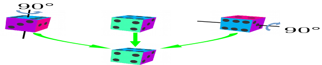
Figure 2: Mapping of 3 ambiguous poses to the same pose. We consider here a uniform object and the colors and dots on the faces are only to visualize the different poses. The left and right poses are remapped to the reference pose in the middle.

As illustrated in Fig. 2, a natural idea to aim at preventing trouble during learning is therefore to first map equivalent rotations to a unique rotation, which we call a canonical rotation. This means that during training, training images with the same object appearance will be assigned the same rotation after mapping. The transformation $\mathcal{F}:\boldsymbol{I}\mapsto\boldsymbol{p}$ of Eq. 2 will thus become a function and we will be able to learn it with a Deep Network for example. This implies that at inference, the network will predict the canonical rotation for a given input image, which is the best that can be done in presence of symmetries.

Given set $\mathcal{M}(O)$ of the object’s proper symmetries, we are therefore looking for an operator $\text{Map}(\cdot)$ on $\text{SO}(3)$ that can map ambiguous 3D rotations to a single rotation such that $\text{Map}(R_{1})=\text{Map}(R_{2})\iff R_{1}\sim R_{2}$ ($\star$) holds.

Proposition 1.

Given a proper symmetry group $\mathcal{M}(O)$, let us define Map operator as:

$$\text{Map}(R)=\hat{S}^{-1}R\>,\quad\forall R\in\text{SO}(3),$$ (3)

with

$$\hat{S}=\operatorname*{arg\,min}_{S\in\mathcal{M}(O)}\|S^{-1}R-I_{3}\|_{F}\>,$$ (4)

where $\|.\|_{F}$ is the Froebenius norm. Then Map verifies the mapping property ($\star$).

Proof.

To simplify the notations, let us consider that $\mathcal{M}(O)$ is made only of the rotation components. By definition of $R_{1}\sim R_{2}$ and $\mathcal{M}(O)$:

$$R_{1}\sim R_{2}\Leftrightarrow\exists!\>S_{12}\in\mathcal{M}(O)\>\>\>\textrm{s.t.}\>\>R_{1}=S_{12}R_{2}\>.$$ (5)

Let us consider the solution of the optimization problem in Eq. (4) for $R_{1}$:

$$\hat{S}_{1}=\operatorname*{arg\,min}_{S\in\mathcal{M}(O)}\|S^{-1}R_{1}-I_{3}\|_{F}\>.$$ (6)

then

$$\hat{S}_{1}=\operatorname*{arg\,min}_{S\in\mathcal{M}(O)}\|S^{-1}S_{12}R_{2}-I_{3}\|_{F}\>.$$ (7)

We introduce variable $T$ such that $S=S_{12}T$. Since $S$ and $S_{12}$ belong to $\mathcal{M}(O)$ and $\mathcal{M}(O)$ is a group, $T$ also belongs to $\mathcal{M}(O)$. We can therefore perform the following change of variable:

$$\hat{S}_{1}=S_{12}\operatorname*{arg\,min}_{T\in\mathcal{M}(O)}\|T^{-1}R_{2}-I_{3}\|_{F}\>,$$ (8)

which is equal to:

$$\hat{S}_{1}=S_{12}\hat{S}_{2}\>,$$ (9)

with

$$\hat{S}_{2}=\operatorname*{arg\,min}_{S\in\mathcal{M}(O)}\|S^{-1}R_{2}-I_{3}\|_{F}\>.$$ (10)

Therefore

$$\begin{array}[]{lcl}R_{1}\sim R_{2}&\Leftrightarrow&\text{Map}(R_{1})=\hat{S}_{1}^{-1}R_{1}=\hat{S}_{2}^{-1}S_{12}^{-1}S_{12}R_{2}\\ &&=\hat{S}_{2}^{-1}R_{2}=\text{Map}(R_{2})\>.\end{array}$$ (11)

∎

3.2 Implementing Map

If $\mathcal{M}$ is discrete, implementing operator Map is trivial, as it is only a matter of iterating over the elements of $\mathcal{M}$ to find the minimum. However, $\mathcal{M}$ can be continuous for some objects. This is the case for generalized cylinders and spheres [2]. For spheres, Map is also trivial as it can always return the identity transformation, for example.

For generalized cylinders, implementing operator Map is more complex. In this case, $\mathcal{M}$ can be written as:

$$\mathcal{M}(O)=\{R^{\boldsymbol{u}}_{\alpha}:\alpha\in[0,2\pi)\},$$ (12)

where $R^{\boldsymbol{u}}_{\alpha}$ is the rotation around axis ${\boldsymbol{u}}$ of amount $\alpha$.

The Froebenius norm in Eq. (4) can be rewritten as

$$\|S^{-1}R-I_{3}\|_{F}=\|D\|_{F}=\text{Trace}(D^{T}D)\>,$$ (13)

with $D=S^{-1}R-I_{3}$. After some derivations:

$$\|S^{-1}R-I_{3}\|_{F}=6-\text{Trace}(S^{T}R)\>.$$ (14)

The complete derivations can be found in the supplementary material.

Without loss of generality, we can assume that ${\boldsymbol{u}}$ is the ${\boldsymbol{z}}$-axis of the object’s coordinate system: If it is not the case, the following still holds after applying a change of basis. Then, $S$ has the following form:

$$S=\begin{bmatrix}\cos(\alpha)&-\sin(\alpha)&0\\ \sin(\alpha)&\cos(\alpha)&0\\ 0&0&1\end{bmatrix}\>,$$ (15)

and, after some basic manipulation:

$$\text{Trace}(D^{T}D)=6 -(R_{11}+R_{22})\cos(\alpha)$$ (16)

$$+(R_{12}-R_{21})\sin(\alpha)\>.$$

To implement Map, we need to solve the optimization problem $\hat{S}=\operatorname*{arg\,min}\limits_{S\in\mathcal{M}(O)}\text{Trace}(D^{T}D)$, which can now be rewritten as a minimization over $\alpha$:

$$\hat{\alpha} =\operatorname*{arg\,min}\limits_{\alpha\in[0,2\pi)}\text{Trace}(D^{T}D)$$ (17)

$$=\operatorname*{arg\,max}\limits_{\alpha\in[0,2\pi)}\>(R_{11}+R_{22})\cos(\alpha)-(R_{12}-R_{21})\sin(\alpha)\>.$$

This is solved analytically by solving $\frac{\partial\text{Trace}(D^{T}D)}{\partial\alpha}=0$ for $\alpha$. The solution of Eq. (4) is then:

$$\hat{S}=R^{\boldsymbol{z}}_{\hat{\alpha}}\quad\textrm{with }\>\>\hat{\alpha}=\text{arctan2}(R_{21}-R_{12},R_{11}+R_{22})\>.$$ (18)

3.3 Discontinuities of $\mathcal{F}$ After Mapping

After applying the Map operator, there are no pose ambiguities anymore, i.e. two similar images are assigned the same rotation. However, a new difficulty arises: The transformation $\mathcal{F}(\boldsymbol{I})\rightarrow\boldsymbol{p}$ is now discontinuous around some rotations. This is problematic when using Deep Networks to learn $\mathcal{F}$, as Deep Networks can only approximate continuous functions [5, 15, 8].

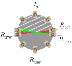
Figure 3: Discontinuities of $\mathcal{F}$ after applying the Map operator, for an object with one axis of symmetry and a $\pi$-symmetry. All poses are mapped to a pose in the hashed region by operator Map introduced in Section 3.1. Since $\text{Map}(R^{z}_{\pi/2+\epsilon})=R^{z}_{\epsilon-\pi/2}$ (visualized by the green arrow) and $\text{Map}(R^{z}_{\pi/2-\epsilon})=R^{z}_{\pi/2-\epsilon}$, there exists a hazardous region (in red) where $\mathcal{F}$ is discontinuous.

To understand why these discontinuities happen, let us consider an example, more exactly the rectangular object seen from the top as in Fig. 3. $\mathcal{M}(O)$ is made of two rotations around the $Z$ axis: The identity matrix, and the rotation of angle $\pi$, and $\mathcal{M}(O)=\{I_{3},R^{\boldsymbol{u}}_{\pi}\}$. If a training image is annotated with rotation $R_{\pi/2+\epsilon}^{\boldsymbol{z}}$, this rotation will be mapped by operator Map to rotation $R_{\epsilon-\pi/2}^{\boldsymbol{z}}$; If a training image is annotated with pose $R_{\pi/2-\epsilon}^{\boldsymbol{z}}$, this rotation will be mapped to itself i.e. $R_{\pi/2-\epsilon}^{\boldsymbol{z}}$. By making $\epsilon$ converge to 0, it can be seen that there is a discontinuity of $\mathcal{F}$ around images annotated with rotations $\pi$ before mapping.

Another way of looking at the problem is to notice that images of the object annotated with rotations $R_{\epsilon-\pi/2}^{\boldsymbol{z}}$ and $R_{\pi/2-\epsilon}^{\boldsymbol{z}}$ look very similar, but with very different rotations. A Deep Network would have to learn to predict very different poses for very similar images.

3.4 Solving the Discontinuities

The discontinuities only occur when $\mathcal{M}$ is discrete: It can be seen from Eq. (18) that in the case of a generalized cylinder, the Map operator is continuous. Otherwise, we avoid these discontinuities by introducing a partition of $\text{SO}(3)$ made of two subsets $\Omega_{1}$ and $\Omega_{2}$. For each subset, we train a different regressor to predict the pose. We will therefore have two regressors $\mathcal{F}_{1}$ and $\mathcal{F}_{2}$ instead of only one. In this way, both $\mathcal{F}_{1}$ and $\mathcal{F}_{2}$ will be continuous over their respective domains.

We describe below our method on an example, and then extend it to the general case.

3.4.1 One Symmetry Axis, $M=2$

Let us consider again the rectangular object pictured in Fig. 3, and already discussed in Section 3.3. For this object, we have $\mathcal{M}(O)=\{I_{3},R^{\boldsymbol{u}}_{\pi}\}$. We can notice that $\mathcal{M}$ and Map generate a partition of $\text{SO}(3)$ made of two subsets:

$$\Omega_{1}=\{R:\hat{S}(R)=I_{3}\}\text{ and }\Omega_{2}=\{R:\hat{S}(R)=R^{\boldsymbol{u}}_{\pi}\}\>,$$ (19)

where $\hat{S}(R)$ is the rotation of Eq. (4) when applying Map to $R$.

However, this partition will not solve our problem: We already know that $\mathcal{F}$ is not continuous on $\Omega_{1}$. We must therefore introduce a new partition of $\text{SO}(3)$. For this partition, we consider the new set:

$$\sqrt{\mathcal{M}}(O) =\{(R^{\boldsymbol{u}}_{k\pi/2}):k\in\mathbb{Z}\}$$ (20)

$$=\{I_{3},R^{\boldsymbol{u}}_{\pi/2},R^{\boldsymbol{u}}_{\pi},R^{\boldsymbol{u}}_{3\pi/2}\}\>,$$

and the partition it generates with Map:

$$\Omega^{(k)}=\{R:\hat{S}(R)=R^{\boldsymbol{u}}_{k\pi/2}\}\>.$$ (21)

As shown in Fig. 4(b), no part $\Omega^{(k)}$ include any discontinuity. Moreover, for a rotation in $\Omega^{(2)}$, there is another rotation in $\Omega^{(0)}$ that generates the same object appearance. The same yields for $\Omega^{(3)}$ and $\Omega^{(1)}$.

We therefore take $\Omega_{1}=\Omega^{(0)}$ for the domain of regressor $\mathcal{F}_{1}$, and $\Omega_{2}=\Omega^{(1)}$ for the domain of regressor $\mathcal{F}_{2}$. $\mathcal{F}_{1}$ and $\mathcal{F}_{2}$ thus do not suffer from discontinuities nor ambiguity. They are sufficient to estimate the object pose under any rotation, since we can map this rotation to a rotation either in $\Omega_{1}$ or $\Omega_{2}$ corresponding to the same appearance. To do so, we introduce a new mapping $\text{Map}^{\prime}$ derived from Map such that:

$$\forall R\in SO(3),\quad\text{Map}^{\prime}(R)=(\hat{S}^{-1}R,\delta)\>\>\textrm{such that }(\hat{S},\delta)=$$ (22)

$$\textrm{\begin{tabular}[]{p{0.95\linewidth}}$\left\{\textrm{\begin{tabular}[]{p{1\linewidth}}$(\operatorname*{arg\,min}\limits_{S\in\mathcal{M}(O)}\|S^{-1}R-I_{3}\|_{F},1)\quad$ if $\text{Map}(R)\in\Omega_{1}$ ,\\ $(\operatorname*{arg\,min}\limits_{S\in\mathcal{M}(O)}\|S^{-1}R-R^{\boldsymbol{u}}_{\pi/2}\|_{F},2)\quad$ otherwise ,\end{tabular}}\right.$\end{tabular}}$$

During training, given a training image $\boldsymbol{I}$ annotated with rotation $R$, we compute $(\hat{S}^{-1}R,\delta)\leftarrow\text{Map}^{\prime}(R)$ and train regressor $\mathcal{F}_{\delta}$ to predict rotation $\hat{S}^{-1}R$ from $\boldsymbol{I}$.

During inference, given a test image $\boldsymbol{I}$ of an object, we need to know which regressor we should invoke to predict the pose. To do so, during training, we train a classifier $\mathcal{C}$ to predict which regressor we should invoke to compute the pose, that is we train $\mathcal{C}$ to predict $\delta$ from $\boldsymbol{I}$. For rotations close to the boundary between $\Omega_{1}$ and $\Omega_{2}$, the prediction for $\mathcal{C}$ can become ambiguous. However, in this case, the ambiguity is not a problem in practice: Even if the classifier predicts the wrong regressor to use close to the boundary between $\Omega_{1}$ and $\Omega_{2}$, both regressors can correctly predict poses close to this boundary.

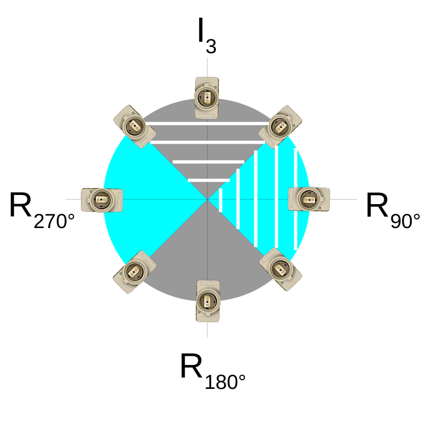
(a)

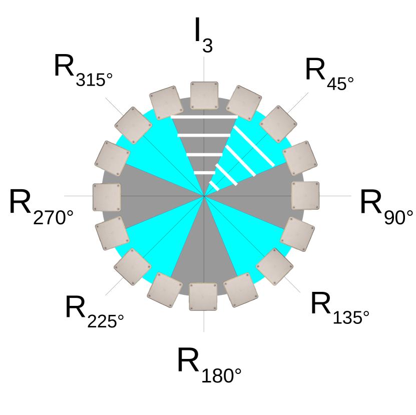
(b)

Figure 4: Partitions for an object with one axis of symmetry with $M=2$ (left) and $M=4$ (right) as defined in Section 3.4. Rotations in areas filled with one color should be mapped to a rotation in the hashed region of same color to avoid discontinuities. Two different regressors $\mathcal{F}_{1}$ and $\mathcal{F}_{2}$, one for each color, are used to predict poses for each hashed region.

3.4.2 One Symmetry Axis, Arbitrary $M$

Let us now generalize to an object $O$ with an arbitrary amount of symmetries around a single axis $u$. These symmetries are necessarily periodic around ${\boldsymbol{u}}$ with angular period $f_{\alpha}=2\pi/M$: Rotating $O$ around $u$ by any angle multiple of $f_{\alpha}$ does not change its appearance. The proper symmetry group $\mathcal{M}(O)$ for such an object is:

$$\mathcal{M}(O)=\left\{\left(R^{\boldsymbol{u}}_{2\pi/M}\right)^{m}\right\}_{m\in\mathbb{N}}=\{R^{\boldsymbol{u}}_{2m\pi/M}\}_{m\in\mathbb{N}}\>.$$ (23)

$\sqrt{\mathcal{M}}(O)$ of Eq. (20)) becomes:

$$\sqrt{\mathcal{M}}(O)=\left\{\left(R^{\boldsymbol{u}}_{\pi/M}\right)^{m}\right\}_{k\in\mathbb{N}}=\{R^{\boldsymbol{u}}_{m\pi/M}\}_{m\in\mathbb{N}}\>,$$ (24)

and mapping $\text{Map}^{\prime}$ of Eq. (22) becomes:

$$\forall R\in SO(3),\quad\text{Map}^{\prime}(R)=(\hat{S}^{-1}R,\delta)\>\>\textrm{such that }(\hat{S},\delta)=$$ (25)

$$\textrm{\begin{tabular}[]{p{0.95\linewidth}}$\left\{\textrm{\begin{tabular}[]{p{1\linewidth}}$(\operatorname*{arg\,min}\limits_{S\in\mathcal{M}(O)}\|S^{-1}R-I_{3}\|_{F},1)\quad$ if $\text{Map}(R)\in\Omega_{1}$ ,\\ $(\operatorname*{arg\,min}\limits_{S\in\mathcal{M}(O)}\|S^{-1}R-R^{\boldsymbol{u}}_{\pi/M}\|_{F},2)\quad$ otherwise ,\end{tabular}}\right.$\end{tabular}}$$

where $\Omega_{1}=\{R:\hat{S}(R)=I_{3}\}$.

We can use $\text{Map}^{\prime}$ the same way as in the previous subsection to train and use to regressors $\mathcal{F}_{1}$ and $\mathcal{F}_{2}$.

3.4.3 General Case

In the general case, each rotation $R$ in $\mathcal{M}$ can be written in the form:

$$R=R_{2\pi/M}^{\boldsymbol{u}}.R_{2\pi/N}^{\boldsymbol{v}}....\quad\textrm{with }M,N,..\in\mathbb{N}\>,$$ (26)

where ${\boldsymbol{u}}$, ${\boldsymbol{v}}$, etc. are rotation axes. Most common objects have at most 2 axes of symmetries, but it is possible to imagine objects with more, for example a golf ball. To keep the notations as simple as possible, we will stick to only two axes, as it is easy to extend to more axes from there.

$\sqrt{\mathcal{M}}(O)$ becomes:

$$\sqrt{\mathcal{M}}(O)=\{R^{\boldsymbol{u}}_{m\pi/M}.R^{\boldsymbol{u}}_{n\pi/N}\}_{(m,n)\in\mathbb{N}^{2}}\>,$$ (27)

and mapping $\text{Map}^{\prime}$ becomes:

$$\forall R\in SO(3),\text{Map}^{\prime}(R)=(\hat{S}^{-1}R,\delta_{1},\delta_{2})\>\>\textrm{s.t. }(\hat{S},\delta_{1},\delta_{2})=$$ (28)

$$\textrm{\begin{tabular}[]{p{0.95\linewidth}}$\left\{\textrm{\begin{tabular}[]{p{1\linewidth}}$(\operatorname*{arg\,min}\limits_{S\in\mathcal{M}(O)}\|S^{-1}R-I_{3}\|_{F},1,1)$ if $\text{Map}(R)\in\Omega_{1,1}$ ,\\ $(\operatorname*{arg\,min}\limits_{S\in\mathcal{M}(O)}\|S^{-1}R-R^{\boldsymbol{u}}_{\pi/M}\|_{F},2,1)$ if $\text{Map}(R)\in\Omega_{2,1}$ ,\\ $(\operatorname*{arg\,min}\limits_{S\in\mathcal{M}(O)}\|S^{-1}R-R^{\boldsymbol{v}}_{\pi/N}\|_{F},1,2)$ if $\text{Map}(R)\in\Omega_{1,2}$ ,\\ $(\operatorname*{arg\,min}\limits_{S\in\mathcal{M}(O)}\|S^{-1}R-R^{\boldsymbol{u}}_{\pi/M}R^{\boldsymbol{v}}_{\pi/N}\|_{F},2,2)$ otherwise ,\end{tabular}}\right.$\end{tabular}}$$

where $\Omega_{1,1}=\{R:\hat{S}(R)=I_{3}\}$, $\Omega_{2,1}=\{R:\hat{S}(R)=R^{\boldsymbol{u}}_{\pi/M}\}$, and $\Omega_{1,2}=\{R:\hat{S}(R)=R^{\boldsymbol{v}}_{\pi/N}\}$. It means that in this case, we have to train 4 different regressors $\mathcal{F}_{1,1}$, $\mathcal{F}_{2,1}$, $\mathcal{F}_{1,2}$, and $\mathcal{F}_{2,2}$ according to $\delta_{1}$ and $\delta_{2}$, and the classifier $\mathcal{C}$ to predict a class index in $[0;3]$.

3.5 Method Summary

The method developed above can be summarized as follow. We distinguish between generalized cylinders and objects with discrete symmetries.

If the object is a generalized cylinder, given a training image $\boldsymbol{I}$ annotated with rotation $R$, we train a single regressor $\mathcal{F}$ to predict $\text{Map}(R)$ using Eq. 3 from $\boldsymbol{I}$. At inference time, given a test image $\boldsymbol{I}$, we simply have to invoke $\mathcal{F}$ to predict the object pose from $\boldsymbol{I}$.

If the object has discrete symmetries, given a training image $\boldsymbol{I}$ annotated with rotation $R$, we apply $\text{Map}^{\prime}$ to $R$ using Eq. (25) or Eq. (28) depending on the number of symmetry axes. $\text{Map}^{\prime}$ provides the rotation to be associated with $\boldsymbol{I}$ for training, as well as the index of the regressor $\mathcal{F}_{i}$ to train. In addition to training the regressors, we need to train classifier $\mathcal{C}$ to predict the index of the regressor to use. At inference time, we first invoke classifier $\mathcal{C}$ to predict which regressor we should use from $\boldsymbol{I}$, and then, invoke this regressor to predict the object pose from $\boldsymbol{I}$.

4 Integration into Faster-RCNN

We integrated our approach into Faster-RCNN [25]. We keep the original architecture of [25] to obtain region proposals and classify each of those regions with an object label: In the T-Less dataset [14], there exist 30 classes of object. We also keep the original loss terms for this part.

We chose to predict the objects’ 6D poses in the form of the 2D reprojections of the 8 corners of the 3D bounding boxes, as in [23, 27, 28, 22] for simplicity. From these 2D reprojections, it is possible to estimate a 6D pose using a P$n$P algorithm [9]. However, our approach is general, and using any other representation of the pose, with quaternions for example, is also possible.

Fig. 5 shows the different branches we added to the original Faster-RCNN architecture. We describe them below.

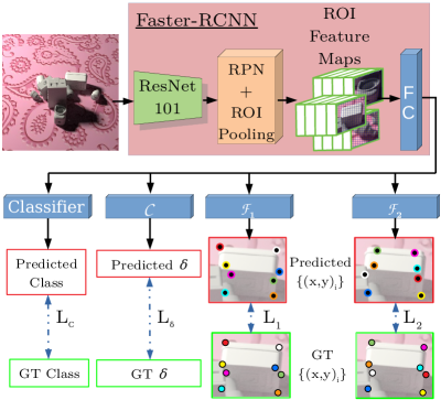
Figure 5: Our architecture for implementing our approach. It is built on top of the Faster-RCNN [25] architecture, to which we add specific branches: One for each regressor $\mathcal{F}_{i}$, and one for classifier $\mathcal{C}$ to learn to choose between the regressors.

Pose regressor $\mathcal{F}$ branch.

We add a specific branch to the Faster-RCNN [25] architecture to predict the 2D coordinates of each 3D corner for each regressor. The output of each branch has size $16\times 30$, where $30$ is the number of object classes and $16$ accounts for the 8 2D coordinates to predict. This branch is implemented as a fully connected multi-layer perceptron and takes as input the output shared single channel feature-map. We then use an $L_{1}$ or $L_{2}$ loss on each coordinate. More details can be found in the supplementary materials.

Classifier $\mathcal{C}$ branch.

We also added a specific multi-layer perceptron branch to Faster-RCNN to implement classifier $\mathcal{C}$. Ground truth is obtained using Eq. (22).

5 Experiments

In this section, we detail how we evaluated our approach, and show its effectiveness on objects with various types of symmetries.

5.1 Dataset

We use the objects of the T-Less dataset [14] as they exhibit many different challenges due to symmetries, and are representative of objects in daily and industrial environments. However, the T-Less dataset does not provide many images for training, with a limited range of poses and illumination conditions. We therefore generated training and test images using the CAD models provided with T-Less, introducing partial occlusions and illumination variations. This dataset is made of 30K samples, generated using the CAD models provided in the original T-Less dataset with Cycles, a photorealistic rendering engine of the open source software Blender.

Each sample of our dataset is generated using a random set $\mathcal{S}$ of objects taken from the T-Less dataset, using random gray scale color (from dark-gray to white) for each of them. Each object of $\mathcal{S}$ is initially set with a random pose, and we let the objects fall down on a randomly textured plane, using Blender’s physics simulator. Because the objects can collide together, their final pose on the table is also random. Illumination randomization is performed by varying the level of ambient light and randomizing a point light source in terms of position, strength, and color. This often results in strong cast shadows, as can be seen in Fig. 6. A comparison with the original T-Less (primesense) dataset is given in Table 1. This dataset therefore provides challenging conditions, and allows us to focus on the challenges raised by the symmetries, without having to consider the domain gap between synthetic and real images.

Dataset	T-Less (primesense)		SyntheT-Less
	Train	Test
Number of samples	38K	10K	30K
Illumination variation	None	Small	Strong
Occlusion	No	Yes	Yes
Multi-objects images	No	Yes	Yes
Object color variation	None	Small	Small
Background variation	None	Small	Strong

Table 1: Comparison between the T-Less dataset and our SyntheT-Less dataset.

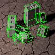
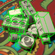
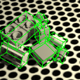
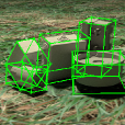
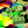
Figure 6: Sample images from our SyntheT-Less dataset. All objects in each image are annotated with their classes and 6D poses.

5.2 Effectiveness of our Approach

As shown in Fig. 9, the loss of our Faster R-CNN -based implementation converges only when the rotations are normalized using our normalization procedure, indicating that something is incorrect in the loss function in absence of normalization. In Fig. 7, we show what happens in practice for three possible types of objects: Two generalized cylinders (objects $30$ and $3$), an object with an axis of symmetry (object $29$), and an object without any symmetry (object $26$). When dealing with non-symmetrical objects, the network is able to learn the 6D pose with and without the normalization procedure. On the opposite, when the objects are symmetrical, without our normalization the network learns the average between all the possible poses ending up predicting a pose collapsed to the center of the object.

(a)	(b)	(c)	(d)

Figure 7: Pose estimation results with (top row) and without (bottom row) our normalization approach for (a) generalized cylinders, (b) an object with an axis of symmetry, (c) an object without any symmetry, and (d) a typical scene from our SyntheT-Less dataset. The green and blue bounding boxes correspond to the ground truth poses estimated poses respectively. Without our normalization, the network learns to predict the average between all the possible poses for symmetrical objects, which is of course meaningless.

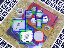
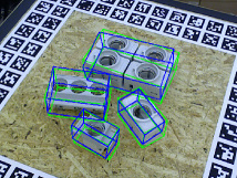
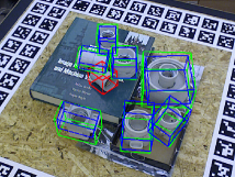
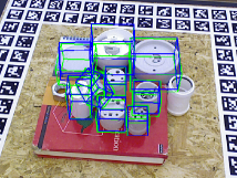
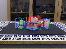
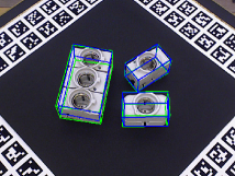
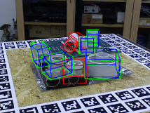
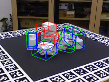
Figure 8: Some qualitative results on test scenes of the T-Less dataset. Green and blue bounding boxes are the ground truth and estimated poses respectively while the red bounding boxes correspond to missed detections.

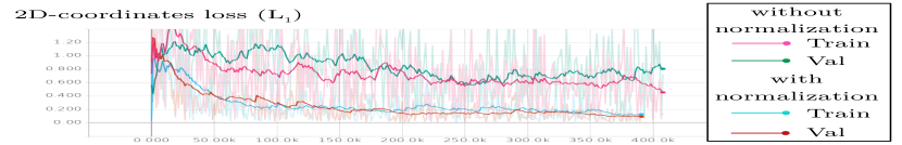
Figure 9: Learning curves on the training and validation sets of our Faster-RCNN based implementation. Without our normalization described in Section 3, the network fails to converge to a satisfying solution. More exactly, it converges to a local minimum where all keypoints collapse at the center of the object—see Fig. 7.

5.3 T-LESS Dataset: Comparison with [26]

We use the Visible Surface Discrepancy (VSD) error function introduced by [13]. It compares the ground truth measured depth maps $\hat{S}$ and the depth maps $\bar{S}$ rendered according to the estimated poses to evaluate the proportion of visible pixels for which the depth absolute discrepancy map $|\hat{S}$ - $\bar{S}|$ is below a threshold $\tau$. As in [13], we set $\tau=20$mm and report the recall of correct 6D object poses at $\mathbf{e_{vsd}<0.3}$. This metric is not sensitive to visual symmetries, as they induce similar symmetries in depth maps.

Table 2 compares our method to the method of Sundermeyer et al [26]. The object 3D orientation and translation along the ${\boldsymbol{x}}$-and ${\boldsymbol{y}}$-axes are typically well estimated. Although most of the translation error is along ${\boldsymbol{z}}$-axis, it is unsurprising since we do not use or regress the depth information. In order to have a meaningful evaluation of our results in terms of VSD, we keep the ground truth of the translation along ${\boldsymbol{z}}$-axis in our pose predictions.

	Sundermeyer et al. [26]				Ours
Object	SSD	Retina	GT BBox		Faster-RCNN
1	5.65	8.87	12.33		26.35
2	5.46	13.22	11.23		56.14
3	7.05	12.47	13.11		83.33
4	4.61	6.56	12.71		32.98
5	36.45	34.80	66.70		44.54
6	23.15	20.24	52.30		98.33
7	15.97	16.21	36.58		87.74
8	10.86	19.74	22.05		17.09
9	19.59	36.21	46.49		52.54
10	10.47	11.55	14.31		5.43
11	4.35	6.31	15.01		27.97
12	7.80	8.15	31.34		43.08
13	3.30	4.91	13.60		48.54
14	2.85	4.61	45.32		42.19
15	7.90	26.71	50.00		47.10
16	13.06	21.73	36.09		42.18
17	41.70	64.84	81.11		56.83
18	47.17	14.30	52.62		19.31
19	15.95	22.46	50.75		27.53
20	2.17	5.27	37.75		32.16
21	19.77	17.93	50.89		41.19
22	11.01	18.63	47.60		49.10
23	7.98	18.63	35.18		26.08
24	4.74	4.23	11.24		41.34
25	21.91	18.76	37.12		44.37
26	10.04	12.62	28.33		23.80
27	7.42	21.13	21.86		33.78
28	21.78	23.07	42.58		35.10
29	15.33	26.65	57.01		15.92
30	34.63	29.58	70.42		36.17
Mean	14.67	18.35	36.79		41.27

Table 2: T-LESS: Object recall for $err_{vsd}<0.3$ on all Primesense test scenes (the higher the better).

6 Conclusion

In this paper, we studied the subtle problems that arise when training a machine learning method to predict the 6D pose of an object with symmetries. This leads to a simple method that is agnostic to the exact pose representation and the pose prediction model. Our method can therefore be included in current and future developments for properly handling objects with symmetries. A direct extension of our work could be to automatically detect the object symmetries.

References

- [1] E. Brachmann, F. Michel, A. Krull, M. Yang, and S. Gumhold. Uncertainty-Driven 6D Pose Estimation of Objects and Scene. In Conference on Computer Vision and Pattern Recognition, 2016.
- [2] R. Brégier, F. Devernay, L. Leyrit, and J. L. Crowley. Defining the Pose of Any 3D Rigid Object and an Associated Distance. International Journal of Computer Vision, 126(6):571–596, June 2018.
- [3] E. Corona, K. Kundu, and S. Fidler. Pose Estimation for Objects with Rotational Symmetry. In International Conference on Intelligent Robots and Systems, 2018.
- [4] A. Crivellaro, M. Rad, Y. Verdie, K. M. Yi, P. Fua, and V. Lepetit. Robust 3D Object Tracking from Monocular Images Using Stable Parts. IEEE Transactions on Pattern Analysis and Machine Intelligence, 2018.
- [5] G. Cybenko. Approximations by Superpositions of Sigmoidal Functions. Mathematics of Control, Signals, and Systems, (4):303–314, 1989.
- [6] T. Do, M. Cai, T. Pham, and I. Reid. Deep-6DPose: Recovering 6D Object Pose from a Single RGB Image. In arXiv Preprint, 2018.
- [7] B. Drost, M. Ulrich, N. Navab, and S. Ilic. Model Globally, Match Locally: Efficient and Robust 3D Object Recognition. In Conference on Computer Vision and Pattern Recognition, 2010.
- [8] B. Hanin. Universal Function Approximation by Deep Neural Nets with Bounded Width and ReLU Activations. In arXiv Preprint, 2017.
- [9] R. Hartley and A. Zisserman. Multiple Views Geometry in Computer Vision. Cambridge University Press, 2000.
- [10] K. He, G. Gkioxari, P. Dollar, and R. Girshick. Mask R-CNN. In International Conference on Computer Vision, 2017.
- [11] P. Henderson and V. Ferrari. Learning to generate and reconstruct 3d meshes with only 2d supervision. In British Machine Vision Conference (BMVC), 2018.
- [12] S. Hinterstoisser, V. Lepetit, S. Ilic, S. Holzer, G. Bradski, K. Konolige, and N. Navab. Model Based Training, Detection and Pose Estimation of Texture-Less 3D Objects in Heavily Cluttered Scenes. In Asian Conference on Computer Vision, 2012.
- [13] T. Hodaň, F. Michel, E. Brachmann, W. Kehl, A. G. Buch, D. Kraft, B. Drost, J. Vidal, S. Ihrke, X. Zabulis, C. Sahin, F. Manhardt, F. Tombari, T.-K. Kim, J. Matas, and C. Rother. BOP: Benchmark for 6D Object Pose Estimation. In European Conference on Computer Vision, pages 19–35, 2018.
- [14] T. Hodaň, P. Haluza, S. Obdržaĺek, J. Matas, M. Lourakis, and X. Zabulis. T-LESS: An RGB-D Dataset for 6D Pose Estimation of Texture-Less Objects. In IEEE Winter Conference on Applications of Computer Vision (WACV), 2017.
- [15] K. Hornik. Approximation Capabilities of Multilayer Feedforward Networks. Neural Networks, 4(2):251–257, 1991.
- [16] O. H. Jafari, S. K. Mustikovela, K. Pertsch, E. Brachmann, and C. Rother. IPose: Instance-Aware 6D Pose Estimation of Partly Occluded Objects. CoRR, abs/1712.01924, 2017.
- [17] W. Kehl, F. Manhardt, F. Tombari, S. Ilic, and N. Navab. SSD-6D: Making RGB-Based 3D Detection and 6D Pose Estimation Great Again. In International Conference on Computer Vision, 2017.
- [18] W. Liu, D. Anguelov, D. Erhan, C. Szegedy, S. E. Reed, C.-Y. Fu, and A. C. Berg. SSD: Single Shot Multibox Detector. In European Conference on Computer Vision, 2016.
- [19] F. Manhardt, D. M. Arroyo, C. Rupprecht, B. Busam, N. Navab, and F. Tombari. Explaining the Ambiguity of Object Detection and 6D Pose from Visual Data. CoRR, abs/1812.00287, 2018.
- [20] F. Manhardt, D. M. Arroyo, C. Rupprecht, B. Busam, N. Navab, and F. Tombari. Explaining the Ambiguity of Object Detection and 6D Pose from Visual Data. In arXiv Preprint, 2019.
- [21] M. Oberweger, M. Rad, and V. Lepetit. Making Deep Heatmaps Robust to Partial Occlusions for 3D Object Pose Estimation. In European Conference on Computer Vision, 2018.
- [22] S. Peng, Y. Liu, Q. Huang, X. Zhou, and H. Bao. PVNet: Pixel-Wise Voting Network for 6DoF Pose Estimation. In Conference on Computer Vision and Pattern Recognition, 2019.
- [23] M. Rad and V. Lepetit. BB8: A Scalable, Accurate, Robust to Partial Occlusion Method for Predicting the 3D Poses of Challenging Objects Without Using Depth. In International Conference on Computer Vision, pages 3848–3856, 2017.
- [24] J. Redmon, S. Divvala, R. Girshick, and A. Farhadi. You Only Look Once: Unified, Real-Time Object Detection. In Conference on Computer Vision and Pattern Recognition, 2016.
- [25] S. Ren, K. He, R. Girshick, and J. Sun. Faster R-CNN: Towards Real-Time Object Detection with Region Proposal Networks. In Advances in Neural Information Processing Systems, 2015.
- [26] M. Sundermeyer, Z. Marton, M. Durner, M. Brucker, and R. Triebel. Implicit 3D Orientation Learning for 6D Object Detection from RGB Images. In European Conference on Computer Vision, 2018.
- [27] B. Tekin, S. N. Sinha, and P. Fua. Real-Time Seamless Single Shot 6D Object Pose Prediction. In Conference on Computer Vision and Pattern Recognition, 2018.
- [28] J. Tremblay, T. To, B. Sundaralingam, Y. Xiang, D. Fox, and S. Birchfield. Deep Object Pose Estimation for Semantic Robotic Grasping of Household Objects. In Conference on Robot Learning (CoRL), 2018.
- [29] Y. Xiang, T. Schmidt, V. Narayanan, and D. Fox. PoseCNN: A Convolutional Neural Network for 6D Object Pose Estimation in Cluttered Scenes. Robotics: Science and Systems Conference, 2018.
- [30] S. Zakharov, I. Shugurov, and S. Ilic. DPOD: Dense 6D Pose Object Detector in RGB Images. In arXiv Preprint, 2019.