P2L: Predicting Transfer Learning
for Images and Semantic Relations
Abstract
We describe an efficient method to accurately estimate the effectiveness of a previously trained deep learning model for use in a new learning task. We use this method, “Predict To Learn” (P2L), to predict the most likely “source” dataset to produce effective transfer for training on a “target” dataset. We validate our approach extensively across 21 tasks, including image classification tasks and semantic relationship prediction tasks in the linguistic domain. The P2L approach selects the best transfer learning model on 62% of the tasks, compared with a baseline of 48% of cases when using a heuristic of selecting the largest source dataset and 52% of cases when using a distance measure between source and target datasets. Further, our work results in an 8% reduction in error rate. Finally, we also show that a model trained from merging multiple source model datasets does not necessarily result in improved transfer learning. This suggests that performance of the target model depends upon the relative composition of the source dataset as well as their absolute scale, as measured by our novel method we term ‘P2L’.
1 Introduction
In deep learning, large number of examples often help capture a robust representation of the unknown input distribution [19] since small data sets may not sufficiently sample the input space. However, in practice, small training jobs are common and labeled data is scarce in many domains. In a survey of industry visual recognition tasks, the users submitted on average 250 images comprising 5 labels per task (see Section 4.3.3).
Our goal is not cross-task transfer. Our aim is to devise a practical and effective guideline for domain adaptation, for intra-task (such as image classification, or relationship prediction) cross-domain transfer, such as transfer from a classification model trained on a subset of ImageNet to a classification model for some unknown image classes related to a problem like industrial defect detection. A motivation is to optimize training of models in a cloud-based vision API.
Inductive transfer learning methods [26, 36] have been identified as a possible solution to this problem. These methods use knowledge acquired in a “source” task to enhance the learning of a new “target” task. However, these methods commonly assume that there is a “best” transfer model, typically the model trained with the largest data set [28]. Yet this assumption stands in tension with results showing that while a well chosen source can improve performance significantly, a poorly chosen source results in worse performance than random initialization [26, 29]. An open challenge remains: for fine-tuning of neural nets, on how to predict the effectiveness of transfer prior to training.
In this work, we describe a method for identifying good transfer models prior to training, that we then validate for commonly used ML tasks in both visual and linguistic domains. A cloud based API which trains deep models for users, for example, must be prepared to train accurate models from widely varied target tasks automatically, while minimizing training time (and computational resources) and maximizing accuracy. Precluding exhaustive search at target task training time, P2L requires only a single forward pass of the target data set through a single reference model to identify, via a predictive algorithm, the most likely candidate for fine-tuning.
In brief, beginning with a single reference model (for images, VGG16 trained on ImageNet1K, and for semantic relations PCNN), we first generate feature vectors for each source dataset. We then use these models to characterize the similarity between source domain features and the target domain’s features. Combining this similarity measure with a non-linear measure of source domain size results in a measure that reflects the source most likely to provide a useful embedding, independent of the larger reference model.
2 Related Work
Transfer learning literature explores a vast number of diverse strategies such as ensemble learning, co-training, model selection, collaborative filtering, few-shot learning [6] [32], domain adaptation [27], weight synthesis [33], and multi-task learning [18] [23] [34] and combinations thereof. Researchers have also investigated practical considerations for domain transfer with limited or incomplete annotations [21] and often suggesting novel learning architectures and optimization objectives effective for such scenarios.
Representation transfer: Representation transfer (RT) learning approaches share a common intuition that compact representations learned from a “source” task can be reused to improve performance on a related “target” task. Instance-based approaches attempt to identify appropriate data used in the source task to supplement target task training, feature-representation approaches attempt to leverage source task weight matrices, and parameter-transfer approaches involve re-using the architecture or hyper-parameters of the source network [9, 26]. These approaches, often supplemented by related small-data techniques such as bootstrapping, can yield improvements in performance (e.g., [4]).
Meta-learning [20] is another approach for representation transfer. While meta-learning typically deals with training a base model on a variety of different learning tasks, transfer learning is about learning from multiple related learning tasks [12]. Efficiency of transfer learning depends on the right source data selection, whereas meta-learning models could suffer from ’negative transfer [26] of knowledge if source and target domains are unrelated.
One approach to RT transfer learning is to leverage existing deep nets trained on other large dataset(s), for example VGG16 [28] for images classification or PCNN [40] for relation prediction. The trained weights in these networks have captured a representation of the input that can be transferred by fine-tuning the weights or retraining the final dense layer of the network on the new task. Most DNN-based RT works assume there is only one source model, usually trained from ImageNet, whereas P2L considers the problem of transfer learning when multiple source models are available.
The Learning to Transfer [37] framework learns a reflection function that transforms feature vector representations to be more effectively classified using a kNN-based approach. Although it uses a model trained on ImageNet to produce the initial feature vectors, it is not a parameter-transfer method, since the selected model is not fine-tuned on the target domains. Our experience is that it is difficult to curate a large number (tens) of prior experiences to adopt this approach in practice.
Fine-tuning variations: Our approach is most similar to that of selective joint fine-tuning [13]. The selective fine-tuning methods typically begin by using low-level features to identify images within a source dataset having similar low-level "textures" to a target dataset. Selective joint fine-tuning concludes by using a multi-task objective to fine-tune the target task using these images. A related approach has been used to enhance performance and reduce training time in document classification [10] and to identify examples to supplement training data [13, 38]. Our goal is to extend this approach to high-level features, and to domains outside computer vision, in order to construct a more complete map of the feature space of a trained network. In this aspect our work has some parallels with “learning to transfer” approaches [35], but it attempts to train a source model optimized for transfer, rather than for target accuracy.
While some recent studies in limited domains have related efficacy of this approach to a similarity between target and source datasets [38], and to the diversity [30] of the examples, few have explored the nature of performance improvement across multiple modalities and across multiple domains in realistic and real world settings. Another recent work [11] uses similarity as a metric for selecting a combination of source models which can be subsequently used for automatically labelling wild data samples, in order to fine-tune source models for a target task. However, it is unclear how these methods perform beyond the few datasets used in their empirical work.
Other Approaches: When transferring information captured by previous task-learning for a new task, it is important to take into account the nature of both tasks. One promising approach involves use of recommender systems (e.g., task2vec [2]) which identify models with similar latent-space representations of labeled data. In multi-task visual learning, a model learned to estimate the similarity space of various visual tasks is used to estimate the degree to which models trained to perform these tasks might contribute to transfer [39]. Our work aims, in part, to combine the low compute cost of the former estimation technique with the enhanced performance of the latter transfer technique, by learning a novel method for selection among previously trained source models.
3 Methods
3.1 Embedding Divergence
Our goal is to make an optimal choice among pre-trained network weights learned for a target task from source tasks . Given a target task and dataset , a model is generated by first training on the source task and dataset , and then this information is transferred to through mechanisms such as fine-tuning. For each pair , performance improvement by transfer in each scenario can be measured by:
| (1) |
where is some defined performance evaluation (such as accuracy), represents the null source task and dataset (that is, the model uses randomly initialized weights), and is the measured performance improvement. Determining the optimal for would then be achieved by optimizing .
However, since exhaustively training every possible model for is computationally expensive, we build a reliable estimator for , whose optimum could be used instead to quickly choose the optimal . Based on extensive experimentation, we propose this estimator, , which we term the “embedding divergence”, as:
| (2) |
where is the size of the source dataset , is a computed “distance” between the target and the source datasets, and is a learned parameter. The standard z-scaling function, defined as is not strictly necessary, but it makes it easier to compare and to display intermediate results.
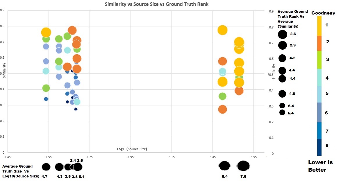
The equation reflects the empirical observation that a larger source dataset tends to generate a more improved target model, and that this improvement tends to grow with size–but only logarithmically [15]. Importantly, the equation also reflects the empirical observation that size alone is an insufficient estimator, and that dissimilarity between the datasets tends to be a negative factor that works against size. As shown in Figure 4, for 9 target datasets over 8 sources (() in section 4), we found that the performance of the target task is strongly correlated with both the similarity of the target dataset with the source, as well as the size of the source dataset itself.
We describe our choice of based on two factors.
First, we represent each dataset by a single, summarizing feature vector, . For example, in our experiments with labeled images, is computed from a convolutional neural network, by extracting for each image the vector produced at a specific layer of the network, and then summarizing the entire dataset by a statistical technique, such as a mean or a trimmed mean. Just as easily, could be computed by another method, such as a future type of reference network, as long as it can represent the entire dataset.
Second, the chosen dissimilarity function must be shown to meaningfully compare the two vectors, being small for “near” datasets, and yet be meaningful for high-dimensional vectors. Candidates for would include Kullback-Leibler or Jensen-Shannon divergence, or Chi-square distance, or a Minkowski metric with (cityblock distance) or (Euclidean distance).
Once we have selected a choice of , the value of can be tuned based on the performance of the approximation function in comparison to the ground truth improvement function . The value of is learned by first training on a collection of target and source datasets, and then evaluating the quality of the estimation on a held-out set of target and source datasets.
Because the exact numeric values of the estimate are not directly comparable with the measures of improvement in , “quality” is defined as how similarly ranks the order of the datasets , compared to the ground truth ranking given by . There are a number of ways to define rank order similarity, many of them based on the non-parametric correlation method of Spearman . We note, however, that it is not necessary to evaluate how well orders the entire collection of possible source datasets ; usually we are only interested in how similarly orders some topmost datasets.
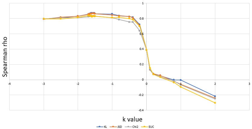
In practice, we have found empirically that (1) the second-last layer of a deep learning network gives good representative vectors for images, (2) averaging these vectors gives a good summary for a dataset, (3) that the choice of distance function is not critical–although KL-divergence and cityblock work well, and (4) that the results are not overly sensitive to the exact choice of (see Figure 1). The optimal choice of for measuring the quality of top-T ranking may depend on the statistical properties of the collection , but it appears to be best if is small.
This work takes an engineering approach to proposing an approximation function . However, this framework is extensible to future work, which may explicitly learn other compact representations of the datasets, other inexpensive dissimilarity functions, and more sophisticated non-linear ways of modeling the observed interaction of size and distance.
3.2 Implementation Details for Images
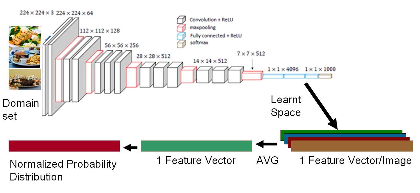
As described in Figure 2, we use as a reference model the VGG16 model pre-trained on ImageNet1K. For , we first extract the response of the penultimate full connection layer, a 4096-dimensional vector. In a learning task with images, we extract such vectors , compute their mean, , and then L1-normalize this mean, giving as the summary feature vector for this task. For , we compute one of several possible distance measures, smoothing any zero components by adding an appropriate value.
3.3 Implementation Details for Semantic Relations
The task of relation prediction provides a second benchmark for source domain selection. In this task, a semantic relations base is extended with information extracted from text. We use the CC-DBP [14] dataset: the text of Common Crawl111http://commoncrawl.org and the semantic relations schema and training data from DBpedia [3]. DBpedia is a knowledge graph extracted from the infoboxes from Wikipedia. An example edge in the DBpedia knowledge graph is , meaning Larry McCray is a blues musician. This relationship is expressed through the DBpedia genre relation, a sub-relation of the high level relation isClassifiedBy. The relation prediction task is to predict the relations, if any, between two nodes in the knowledge graph from the entire set of textual evidence, rather than from each sentence separately as in mention-level relation extraction.
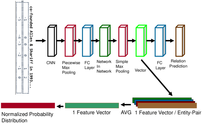
Figure 3 shows the relation prediction neural architecture. The feature representations are taken from the penultimate layer, the max-pooled network-in-network. All models have the same architecture and hyperparameters.
4 Experimental Results and Analysis
4.1 Experimental Approach: Images
For evaluating P2L we used Caltech-UCSD Birds (CUBS) [8], Stanford Cars (Cars) [17], Sketches [22], Wikiart [31] and Oxford Flowers (Oxford) [24] and 9 datasets from the Visual Decathlon Challenge [1]: Aircraft, CIFAR100, Daimler Pedestrian Classification (Daimler), Describable Textures (DTD), German Traffic Sign (GTSRB), Omniglot, Street View House Number (SVHN), UCF101, VGG-Flowers. These 14 datasets, representing fine grained classification tasks, serve as targets () for our evaluation.
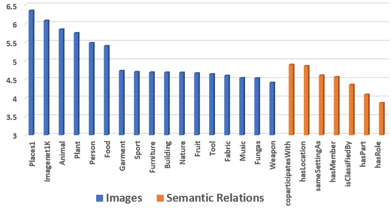
For source datasets (), we used Places1 [5], ImageNet1K [25] and 15 subsets from ImageNet22K [16]. ImageNet22K contains 21,841 categories spread across hierarchical categories such as person, animal, fungus etc. We extracted some of the major hierarchies from ImageNet22K (Fig 5) to form multiple source image sets for our evaluation. A total of 9 million images were used. Some of the domains like animal, plant, person, and food contained substantially more images (and labels) than others categories such as weapon, tool, or sport . This skew is reflective of real world situations, and provides a natural test bed when comparing training sets of different sizes. This is visible in Fig 5
Each of these ImageNet22K domains was then split into four equal partitions. The first was used to train the source model, and the second was used to validate the source model. One-tenth of the third partition was used to create a transfer learning target and the fourth partition was used to validate it. For example, the person hierarchy has more than one million images. This was split into four equal partitions of more than 250K each. The source model was trained with data of that size, whereas the target model was fine-tuned with one-tenth of that data size taken from one of the partitions. These smaller target datasets are reflective of real transfer learning tasks. We thus generated 15 source training datasets and 15 possible target training datasets from ImageNet22K. The 15 source datasets were used, along with Places1 and ImageNet1K, as source datasets for transfer learning.
To tune in our approximation function ( Equation 2), as well as to determine which dissimilarity measure to use, 9 of the target training tasks generated from ImageNet22K were used as a training group, (). These consisted of furniture, food, person, nature, music, fruit, fabric, tool, and building. The value thus generated was used for evaluation on the workloads in the 14 target tasks (referred to above as ), as well as 7 tasks for Semantic Relations.
The training of the source and target models was done using Caffe using a ResNet-27 model. The source models were trained using SGD as in [7] for 900,000 iterations with a step size of 300,000 iterations and an initial learning rate of 0.01. The target models were trained with an identical network architecture, but with a training method with one-tenth of both iterations and step size. A fixed random seed was used throughout all training.
4.2 Experimental Approach: Semantic Relations
We split the task of relation prediction into seven subtasks composed of the high-level relations with the most positive examples in the CC-DBP; other relations were discarded. This was intended to mirror the partitions of ImageNet by high-level classes. The seven source domains () are shown in Figure 5. A model is trained for each of these domains on the full training data for the relevant relation types.
Our approach to transfer learning was the same as in images: a deep neural network trained on the source domain was fine-tuned on the target domain. Fine-tuning involves re-initializing and re-sizing the final layer, since different domains have different numbers of relations. The final layer is updated at the full learn rate , while the previous layers are updated at , with . We used a fine-tune multiplier of .
A new, small training set is built for each target task. For each split of CC-DBP, we take 20 positive examples for each relation from the full training set. (If the total examples is fewer than 20, we take all the training examples.) We then sample ten times as many negatives (i.e., unrelated pairs of entities). These form the target training sets (). The model trained from the full training data of each of the different subtasks is then fine-tuned on the target domain. We measure the area under the precision-recall (PR) curve for each trained model. We also measure the area under the PR curve for a model trained without transfer learning.
4.3 Results
When training a model, we compare our P2L method against five baseline methods of initializing training weights:
1. Source model trained on largest dataset (B1) like in [15]
2. Source model trained on ImageNet1K (B2) for images.
3. Randomly chosen source model from set of models (B3).
4. No transfer learning: weights initialized randomly (B4).
5. Source model trained on least divergent dataset (B5)
We have used this to compare P2L across two domains: Images (Section 4.3.1) and Semantic Relations (Section 4.3.2).
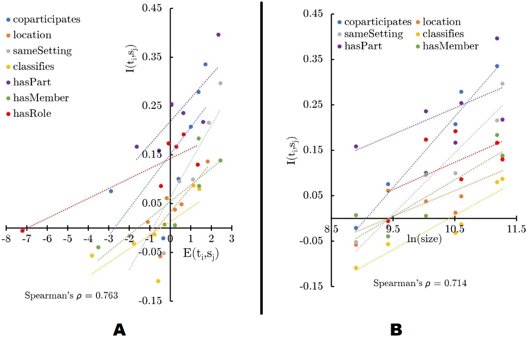
In summary, as shown in Table 1 across 21 tasks in the above two contexts, P2L was able to deliver an average accuracy of 67.22% compared to 64.47% and 64.86%for the baseline method of picking the largest dataset (B1) and most convergent (B5). Additionally, P2L was able to pick a better model in 13 out of 21 tasks. In three tasks where it did not pick the best, the prediction scores between its pick and the winner were very close. The Spearman correlation between the ground truth and the predictions over all the possible source datasets was strong for images (0.707) as shown in Table 2 and semantic relations (0.763) as shown in Fig 6.
Tables 3 and 4 show the relative increase in final performance for our proposed method in comparison to each of these three methods, across images and relations. In the case of images, we present a comparison against ImageNet1K also in Table 3, since ImageNet1K is often used as a source dataset for transfer learning.
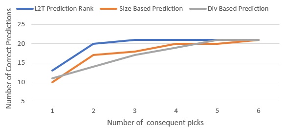
Additionally in Figure 7, we see that P2L is able to pick the best source model for the 21 tasks in maximum of 3 picks from the basket of source models. In contrast, the largest dataset method (B1) would take 6 picks and the most convergent (B5) would take 5 picks.
The latency of a prediction is low. For a dataset like DTD it was 65 seconds on a K40 GPU end to end. In contrast, a training run on DTD takes 43200 secs on the GPU. The prediction latency is largely a function of the number of images in the target dataset. Processing speed for a prediction over 17 source datasets was 30 images/second.
4.3.1 Validation on Image space
We tested distance measures based on Kullback-Leibler Divergence (KLD), Jensen-Shannon Divergence (JSD), Chi-square (CHI2), and Euclidean distance (ED). For each training task in (), we calculated the rank-correlation (Spearman ) between the predictions of each of these measures, and the ground-truth transfer performance based on Top-1 classification accuracy. This is shown in Figure1
This parameter selection of is essentially offline, and only needs to be done once. The same value of is used for images as well as semantic relations.
| Domain | Mean Top-1 Accuracy | Mean Spearman Correlation | ||||
| P2L | Largest | Least | P2L | Largest | Least | |
| (ours) | Dataset | Divergent | (ours) | Dataset | Divergent | |
| Images (14 tasks) | 65.57 | 61.40 | 64.11 | 0.703 | 0.685 | 0.532 |
| Semantic Relations (7 tasks) | 71.79 | 70.6 | 66.36 | 0.763 | 0.714 | 0.037 |
| Average over 21 tasks | 67.22 | 64.47 | 64.86 | 0.723 | 0.695 | 0.367 |
| Target | Spearman | Target | Spearman | |
|---|---|---|---|---|
| Dataset | Dataset | |||
| CUBS | 0.821 | Sketches | 0.843 | |
| VGG-Flowers | 0.630 | Daimler | 0.652 | |
| UCF101 | 0.777 | Omniglot | 0.525 | |
| Oxford | 0.718 | GTSRB | 0.520 | |
| Aircraft | 0.608 | SVHN | 0.603 | |
| DTD | 0.951 | Wikiart | 0.8407 | |
| Cars | 0.64951 | CIFAR100 | 0.730 |
4.3.2 Validation on Common Crawl - DBpedia
Figure 6A shows the correlation of the prediction with the improvement , when using KLD in addition to sizes of the source domains’ training set in . Figure 6B shows the same when only size is used. Using the estimator produced better predictions, that is, and were then better correlated (Spearman = .763). Additionally the overall accuracy obtained using P2L at 71.79% was higher than the overall accuracy obtained using just size at 70.6%.
| Target Dataset | P2L Picked | Largest Training | Least | ImageNet1K | Random Dataset | No Transfer |
|---|---|---|---|---|---|---|
| Best | Dataset | Divergent | Selection | Selection | Learning | |
| Dataset ? | (P2L-B1)/B1 | (P2L-B5)/B5 | (P2L-B2)/B2 | (P2L-B3)/B3 | (P2L-B4)/B4 | |
| CUBS | Yes | 1.00 | 0.00 | 0.28 | 1.69 | 4.28 |
| VGG-Flowers | Yes | 0.57 | 0.00 | 0.21 | 0.82 | 2.13 |
| UCF101 | Yes | 0.00 | 0.00 | 0.08 | 0.47 | 1.77 |
| Oxford | Yes | 0.19 | 0.00 | 0.08 | 0.58 | 1.30 |
| Aircraft | Yes | 0.00 | 0.00 | 0.01 | 0.67 | 0.55 |
| Sketches | Yes | 0.08 | 0.17 | 0.00 | 0.17 | 7.26 |
| Daimler | Yes | 0.00 | 0.00 | 0.00 | 0.00 | 0.01 |
| Omniglot | Yes | 0.00 | 0.00 | 0.00 | 0.07 | 0.27 |
| GTSRB | Yes | 0.00 | 0.00 | 0.00 | 0.00 | 0.01 |
| SVHN | No | -0.01 | 0.00 | 0.00 | 0.02 | 0.02 |
| DTD | No | 0.00 | 0.60 | -0.03 | 0.55 | 2.25 |
| Wikiart | No | 0.00 | -0.04 | -0.04 | 0.79 | 1.31 |
| Cars | No | 0.00 | 0.00 | -0.04 | 0.52 | 2.56 |
| CIFAR100 | No | 0.00 | -0.06 | -0.06 | 0.30 | 4.20 |
| Target Dataset | P2L Picked | Largest Training | Random Dataset | No Transfer |
|---|---|---|---|---|
| Best Dataset? | Dataset | Selection | Learning | |
| (L2T-B1)/B1 | (P2L-B3)/B3 | (P2L-B4)/B4 | ||
| hasPart | Yes | 0.15 | 0.13 | 0.40 |
| copartWith | Yes | 0.00 | 0.14 | 0.34 |
| sameSettingAs | Yes | 0.00 | 0.17 | 0.30 |
| hasLocation | Yes | 0.00 | 0.09 | 0.14 |
| hasMember | No | 0.00 | 0.07 | 0.14 |
| hasRole | No | 0.00 | 0.01 | 0.13 |
| isClassifiedBy | No | -0.01 | 0.08 | 0.08 |
4.3.3 Comparing Against Merged Source Datasets
To help put these results in context, we have investigated how well a merged dataset of various source domains could do in comparison to its individual components. While it may seem that a single merged dataset would perform as well or better than individual sources, in reality we have noticed results to the contrary.
We built a combined dataset of ImageNet22K and Places2 into one large dataset (referred to as LC) and trained a ResNet27 model with it. We then took 71 training datasets submitted by users to a custom learning cloud API, and performed transfer learning experiments from models trained on LC and ImageNet1K. Given that ImageNet1K is a subset of ImageNet22K, it is a subset of LC too. The transfer experiments were done using 8 different learning rate regimes.
For our experiments, we randomly split each set of images with labels into 80% for fine-tuning and 20% for validation. For these 71 training sets, we had a total of approximately 18,000 images: an average of 204 training images and 50 held-out validation images each. There were 5.2 classes per classifier on average, with 2 to 60 classes per classifier.
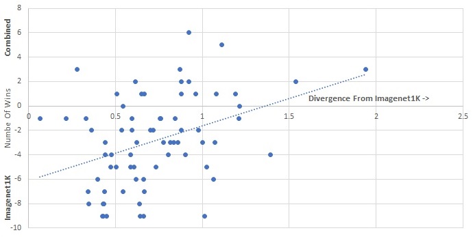
As seen in Figure 8, the large dataset LC did not always win. For training datasets which were closer in divergence to ImageNet1K, the model trained on it was a better base for transfer learning overall. As the task data diverged more and more from ImageNet1K, LC won more and more. In Figure 8, the x-axis denotes the divergence of the task data from ImageNet1K and the y-axis denotes the number of times either LC or ImageNet1K was winner over the 8 learning rate regimes which were tried for each task. Thus the y-axis values range from 8, denoting when the combined dataset won for all the learning rates tried, to -8, denoting when ImageNet1K won.
The likely reason is that, although merging datasets certainly increases size, the merged data is also more diverse and tends to have higher divergence. This empirical result further supports our observations that when considering an individual source dataset, or a merged dataset, or an augmented source dataset, one needs to carefully consider both indicators of the final performance: the size of the effective source dataset, and its divergence with the target dataset.
5 Future Work
The current P2L approach estimates transfer performance at the level of large conceptual categories (e.g.,"animal", or "location"). However, large labeled data sets, such as those used in ImageNet1K, contain deep hierarchies (e.g., animal mammal cat cheetah) that may help to characterize finer resolution maps of the feature space. Identifying crucial sub-features can assist further in selecting more specific source categories, and in developing more efficient source models and transfer techniques.
We currently use only one modality in isolation for determining which source model to use. However, there is significant other information like accompanying test or audio besides the visual (or the semantic relations) which could additionally aid in determining a good source model. For example, blight is a crop disease and crops are more likely to occur in a plant dataset than any other dataset. If one can determine such links from external datasets, they could help choose the best source. Additionally, extracted tags, or other kinds of semantic information extracted from a knowledge graph, can be expected to yield substantial improvements.
Our current P2L method is focused on a single vector characterization of the relationship of source and target datasets (i.e., similarity). We plan to extend our study to explore a more complex model, both of the representation of the datasets, as well as oc more enriched relationships. For example, dispersion statistics of the datasets may be provide further insights into predicting efficacy of the transfer.
6 Conclusions
We described an efficient method for fine-tuning a candidate from a family of pretrained models, applicable to both the image and semantic relations. We conducted an empirical test of the method using models trained on specific conceptual categories across images and semantic relations, demonstrating improved transfer learning results, outperforming baselines such as picking the model trained with the largest data set, or a distance measure between source and target or using a common industry standard model like ImageNet1K. These findings suggest that a learned representation from previous tasks can be used to select the best transfer candidate in order to get greater transfer learning.
Despite order of magnitude differences in training set sizes, we were able to obtain transfer gains by computing an estimate of conceptual closeness. Although prior work has described a saturating curve for training set size contributions to accuracy [19]–a curve which we also observed in our data–we showed that feature similarity provided transfer benefits not predicted by dataset size alone.
Our method is efficient at training and classification time, and has been shown to improve accuracy versus the baseline, both on publicly available image and semantic relations datasets. These results help to explain the tension in the literature between results showing that larger datasets usually outperform smaller, [28], but that ill-selected transfer models can nonetheless degrade performance [29].
Our results suggest that rather than there being a single “best” transfer model, transfer performance critically depends upon the similarity between the source and target models besides the size. Further, methods such as P2L can map the degree of overlap between disparate tasks to select more optimal models. Exploring these “maps” of feature space similarities could be a valuable future direction for deep learning research.
References
- [1] L. Zitnick K. He A. Torralba, K. Murphy. Visual domain decathlon. In PASCAL in Detail Workshop Challenge, CVPR , July 26th, Honolulu, Hawaii, USA. IEEE, 2017.
- [2] Rahul Tewari Avinash Ravichandran Subhransu Maji Charless Fowlkes Stefano Soatto Pietro Perona Alessandro Achille1, Michael Lam. Task2vec: Task embedding for meta learning. arXiv preprint arXiv:1902.03545, 2019.
- [3] Sören Auer, Christian Bizer, Georgi Kobilarov, Jens Lehmann, and Zachary Ives. Dbpedia: A nucleus for a web of open data. In In 6th Int’l Semantic Web Conference, Busan, Korea, pages 11–15. Springer, 2007.
- [4] Hossein Azizpour, Ali Sharif Razavian, Josephine Sullivan, Atsuto Maki, and Stefan Carlsson. Factors of Transferability for a Generic ConvNet Representation. In IEEE Transactions on Pattern Analysis and Machine Intelligence, volume 38, pages 1790–1802, 2016.
- [5] J. Xiao A. Torralba B. Zhou, A. Lapedriza and A. Oliva. Learning deep features for scene recognition using places database. Proc. Advances Neural Inf. Process, 2014.
- [6] Danushka Bollegala, Yutaka Matsuo, and Mitsuru Ishizuka. Relation adaptation: learning to extract novel relations with minimum supervision. In Proceedings of the Twenty-Second international joint conference on Artificial Intelligence-Volume Volume Three, pages 2205–2210. AAAI Press, 2011.
- [7] Léon Bottou. Stochastic gradient tricks. In Grégoire Montavon, Genevieve B. Orr, and Klaus-Robert Müller, editors, Neural Networks, Tricks of the Trade, Reloaded, Lecture Notes in Computer Science (LNCS 7700), pages 430–445. Springer, 2012.
- [8] P. Welinder P. Perona C. Wah, S. Branson and S. Belongie. The caltech-ucsd birds-200-2011 dataset. 2011.
- [9] Wenyuan Dai, Qiang Yang, Gui-Rong Xue, and Yong Yu. Boosting for transfer learning. Intl Conf on Machine Learning, pages 193–200, 2007.
- [10] Arindam Das, Saikat Roy, and Ujjwal Bhattacharya. Document Image Classification with Intra-Domain Transfer Learning and Stacked Generalization of Deep Convolutional Neural Networks. 2018.
- [11] Parijat Dube, Bishwaranjan Bhattacharjee, Siyu Huo, Patrick Watson, Brian Belgodere, and John R Kender. Automatic labeling of data for transfer learning. nature, 192255:241, 2019.
- [12] Chelsea Finn, Pieter Abbeel, and Sergey Levine. Model-agnostic meta-learning for fast adaptation of deep networks. CoRR, abs/1703.03400, 2017.
- [13] Weifeng Ge and Yizhou Yu. Borrowing treasures from the wealthy: Deep transfer learning through selective joint fine-tuning. In Proc. IEEE Conference on Computer Vision and Pattern Recognition, Honolulu, HI, volume 6, 2017.
- [14] Michael Glass and Alfio Gliozzo. A Dataset for Web-scale Knowledge Base Population. In Proceedings of the 15th Extended Semantic Web Conference, 2018.
- [15] Joel Hestness, Sharan Narang, Newsha Ardalani, Gregory F. Diamos, Heewoo Jun, Hassan Kianinejad, Md. Mostofa Ali Patwary, Yang Yang, and Yanqi Zhou. Deep learning scaling is predictable, empirically. CoRR, abs/1712.00409, 2017.
- [16] R. Socher L.-J. Li K. Li J. Deng, W. Dong and L. Fei-Fei. Imagenet: A large-scale hierarchical image database. IEEE Computer Vision and Pattern Recognition (CVPR), 2009.
- [17] J. Deng J. Krause, M. Stark and L. Fei-Fei. 3D object representations for fine-grained categorization. In In ICCV Workshop on Workshop on 3D Representation and Recognition, 2013.
- [18] Jing Jiang. Multi-task transfer learning for weakly-supervised relation extraction. In 4th International Joint Conference on Natural Language Processing. Association for Computational Linguistics, 2009.
- [19] Taskin Kavzoglu and Ismail Colkesen. The effects of training set size for performance of support vector machines and decision trees. Symposium on Spatial Accuracy Assessment in Natural Resources, 2012.
- [20] Christiane Lemke, Marcin Budka, and Bogdan Gabrys. Metalearning: a survey of trends and technologies. Artificial Intelligence Review, 44(1):117–130, Jun 2015.
- [21] Zelun Luo, Yuliang Zou, Judy Hoffman, and Li Fei-Fei. Label efficient learning of transferable representations across domains and tasks. In NIPS, 2017.
- [22] J. Hays M. Eitz and M. Alexa. How do humans sketch objects? ACM Transactions on Graphics, 31(4):44–1, 2012.
- [23] Thien Huu Nguyen, Lisheng Fu, Kyunghyun Cho, and Ralph Grishman. A Two-stage Approach for Extending Event Detection to New Types via Neural Networks. ACL Representation Learning for NLP Workshop, 2016.
- [24] M.-E. Nilsback and A. Zisserman. Automated flower classification over a large number of classes. In In Indian Conference on Computer Vision, Graphics & Image Processing, 2008.
- [25] Hao Su Jonathan Krause Sanjeev Satheesh Sean Ma Zhiheng Huang Andrej Karpathy Aditya Khosla Michael Bernstein Alexander C. Berg Li Fei-Fei Olga Russakovsky, Jia Deng. Imagenet large scale visual recognition challenge. International Journal of Computer Vision, 2015.
- [26] Sinno Jialin Pan and Qiang Yang. A Survey on Transfer Learning. IEEE Transactions on knowledge and data engineering, 22(10):1–15, 2010.
- [27] Novi Patricia and Barbara Caputo. Learning to learn, from transfer learning to domain adaptation: A unifying perspective. Conference on Computer Vision and Pattern Recognition, 2014.
- [28] Ali Sharif Razavian, Hossein Azizpour, Josephine Sullivan, and Stefan Carlsson. CNN features off-the-shelf: an astounding baseline for recognition. CoRR, abs/1403.6382, 2014.
- [29] Michael T Rosenstein, Zvika Marx, Leslie Pack Kaelbling, and Thomas G Dietterich. To transfer or not to transfer. In NIPS 2005 workshop on transfer learning, 2005.
- [30] Sebastian Ruder and Barbara Plank. Learning to select data for transfer learning with bayesian optimization. CoRR, abs/1707.05246, 2017.
- [31] B. Saleh and A. Elgammal. Large-scale classification of fineart paintings: Learning the right metric on the right feature. 2015.
- [32] Richard Socher, Milind Ganjoo, Hamsa Sridhar, Osbert Bastani, Christopher D. Manning, and Andrew Y. Ng. Zero-Shot Learning Through Cross-Modal Transfer. pages 935–943, 2013.
- [33] David Sussillo and L. Abbott. Transferring learning from external to internal weights in Echo-State networks with sparse connectivity. PLoS ONE, 2012.
- [34] Lisa Torrey and Jude Shavlik. Transfer learning. In Handbook of research on machine learning applications and trends: algorithms, methods, and techniques, pages 242–264. IGI Global, 2010.
- [35] Ying Wei, Yu Zhang, and Qiang Yang. Learning to transfer. CoRR, abs/1708.05629, 2017.
- [36] Karl Weiss, Taghi M. Khoshgoftaar, and DingDing Wang. A survey of transfer learning. Journal of Big Data, 3(1):9, May 2016.
- [37] Wei Ying, Yu Zhang, Junzhou Huang, and Qiang Yang. Transfer learning via learning to transfer. In International Conference on Machine Learning, pages 5072–5081, 2018.
- [38] Jason Yosinski, Jeff Clune, Yoshua Bengio, and Hod Lipson. How transferable are features in deep neural networks? In NIPS, 2014.
- [39] Amir Roshan Zamir, Alexander Sax, William B. Shen, Leonidas J. Guibas, Jitendra Malik, and Silvio Savarese. Taskonomy: Disentangling task transfer learning. CoRR, abs/1804.08328, 2018.
- [40] Daojian Zeng, Kang Liu, Yubo Chen, and Jun Zhao. Distant supervision for relation extraction via piecewise convolutional neural networks. In EMNLP, pages 1753–1762, 2015.