Iterative Linearized Control:
Stable Algorithms and Complexity Guarantees

Abstract

We examine popular gradient-based algorithms for nonlinear control in the light of the modern complexity analysis of first-order optimization algorithms. The examination reveals that the complexity bounds can be clearly stated in terms of calls to a computational oracle related to dynamic programming and implementable by gradient back-propagation using machine learning software libraries such as PyTorch or TensorFlow. Finally, we propose a regularized Gauss-Newton algorithm enjoying worst-case complexity bounds and improved convergence behavior in practice. The software library based on PyTorch is publicly available.

Introduction

Finite horizon discrete time nonlinear control has been studied for decades, with applications ranging from spacecraft dynamics to robot learning (Bellman, 1971; Whittle, 1982; Bertsekas, 2005). Popular nonlinear control algorithms, such as differential dynamic programming or iterative linear quadratic Gaussian algorithms, are commonly derived using a linearization argument relating the nonlinear control problem to a linear control problem (Todorov & Li, 2003; Li & Todorov, 2007).

We examine nonlinear control algorithms based on iterative linearization techniques through the lens of the modern complexity analysis of first-order optimization algorithms. We first reformulate the problem as the minimization of an objective that is written as a composition of functions. Owing to this reformulation, we can frame several popular nonlinear control algorithms as first-order optimization algorithms applied to this objective.

We highlight the equivalence of dynamic programming and gradient back-propagation in this framework and underline the central role of the corresponding automatic differentiation oracle in the complexity analysis in terms of convergence to a stationary point of the objective. We show that the number of calls to this automatic differentiation oracle is the relevant complexity measure given the outreach of machine learning software libraries such as PyTorch or TensorFlow (Paszke et al., 2017; Abadi et al., 2015).

Along the way we propose several improvements to the iterative linear quadratic regulator (ILQR) algorithm, resulting in an accelerated regularized Gauss-Newton algorithm enjoying a complexity bound in terms of convergence to a stationary point and displaying stable convergence behavior in practice. Regularized Gauss-Newton algorithms give a template for the design of algorithms based on partial linearization with guaranteed convergence (Bjorck, 1996; Burke, 1985; Nesterov, 2007; Lewis & Wright, 2016; Drusvyatskiy & Paquette, 2018). The proposed accelerated regularized Gauss-Newton algorithm is based on a Gauss-Newton linearization step stabilized by a proximal regularization and boosted by a Catalyst extrapolation scheme, potentially accelerating convergence while preserving the worst-case guarantee.

Related work.

Differential dynamic programming (DDP) and iterative linearization algorithms are popular algorithms for finite horizon discrete time nonlinear control (Tassa et al., 2014). DDP is based on approximating the Bellman equation at the current trajectory in order to use standard dynamic programming. Up to our knowledge, the complexity analysis of DDP has been limited; see (Mayne, 1966; Jacobson & Mayne, 1970; Todorov & Li, 2003) for classical analyses of DDP.

Iterative linearization algorithms such as the iterative linear quadratic regulator (ILQR) or the iterative linearized Gaussian algorithm (ILQG) linearize the trajectory in order to use standard dynamic programming (Li & Todorov, 2004; Todorov & Li, 2005; Li & Todorov, 2007). Again, the complexity analysis of ILQR for instance has been limited. In this paper, we refer to the definitions of ILQR and ILQG as given in the original papers (Li & Todorov, 2004; Todorov & Li, 2005; Li & Todorov, 2007), the same names have been then used for variants of those algorithms that use a roll-out phase on the true trajectory as in, e.g., (Tassa et al., 2012) where line-searches were proposed. Line-searches akin to the Levenberg-Marquardt method were proposed but without convergence rates (Todorov & Li, 2005). It is worthwhile to mention related approaches in the nonlinear model predictive control area (Grüne & Pannek, 2017; Richter et al., 2012; Dontchev et al., 2018).

We adopt the point of view of the complexity theory of first-order optimization algorithms. The computation of a Gauss-Newton step (or a Newton step) through dynamic programming for nonlinear control problems is classical; see (Whittle, 1982; Dunn & Bertsekas, 1989; Sideris & Bobrow, 2005). However, while the importance of the addition of a proximal term in Gauss-Newton algorithms is now well-understood (Nesterov, 2007), several popular nonlinear control algorithms involving such steps, such as ILQR, have not been revisited yet (Li & Todorov, 2004). Our work shows how to make these improvements.

We also show how gradient back-propagation, i.e., automatic differentiation (Griewank & Walther, 2008), a popular technique usually derived using either a chain rule argument or a Lagrangian framework (Bertsekas, 2005; LeCun et al., 1988), allows one to solve the dynamic programming problems arising in linear quadratic control. Consequently, the subproblems that arise when using iterative linearization for nonlinear control can be solved with calls to an automatic differentiation oracle implementable in PyTorch or TensorFlow (Abadi et al., 2015; Paszke et al., 2017; Kakade & Lee, 2018).

The regularized Gauss-Newton method was extensively studied to minimize the nonlinear least squares objectives arising in inverse problems (Bjorck, 1996; Nocedal & Wright, 2006; Kaltenbacher et al., 2008; Hansen et al., 2013). The complexity-based viewpoint used in (Nesterov, 2007; Cartis et al., 2011; Drusvyatskiy & Paquette, 2018) informs our analysis and offers generalizations to locally Lipschitz objectives. We build upon these results in particular when equipping the proposed regularized Gauss-Newton algorithm with an extrapolation scheme in the spirit of (Paquette et al., 2018).

All notations are presented in Appendix A. The code for this project is available at https://github.com/vroulet/ilqc.

1 Discrete time control

We first present the framework of finite horizon discrete time nonlinear control.

Exact dynamics.

Given state variables $x\in{\mathbb{R}}^{d}$ and control variables $u\in{\mathbb{R}}^{p}$, we consider the control of finite trajectories $\bar{x}=(x_{1};\ldots;x_{\tau})\in{\mathbb{R}}^{\tau d}$ of horizon $\tau$ whose dynamics are controlled by a command $\bar{u}=(u_{0};\ldots;u_{\tau-1})\in{\mathbb{R}}^{\tau p}$, through

$$x_{t+1}=\phi_{t}(x_{t},u_{t}),\qquad\mbox{for $t=0,\ldots,\tau-1$,}$$ (1)

starting from a given $\hat{x}_{0}\in{\mathbb{R}}^{d}$, where the functions $\phi_{t}:{\mathbb{R}}^{d}\times{\mathbb{R}}^{p}\rightarrow{\mathbb{R}}^{d}$ are assumed to be differentiable.

Optimality is measured through convex costs $h_{t}$, $g_{t}$, on the state and control variables $x_{t}$, $u_{t}$ respectively, defining the discrete time nonlinear control problem

$$\min_{\begin{subarray}{c}x_{0},\ldots,x_{\tau}\in{\mathbb{R}}^{d}\\ u_{0},\ldots,u_{\tau-1}\in{\mathbb{R}}^{p}\end{subarray}}\quad \sum_{t=1}^{\tau}h_{t}(x_{t})+\sum_{t=0}^{\tau-1}g_{t}(u_{t})$$ (2)

subject to $$x_{t+1}=\phi_{t}(x_{t},u_{t}),\qquad x_{0}=\hat{x}_{0},$$

where, here and thereafter, the dynamics must be satisfied for $t=0,\ldots,\tau-1$.

Noisy dynamics.

The discrepancy between the model and the dynamics can be taken into account by considering noisy dynamics as

$$x_{t+1}=\phi_{t}(x_{t},u_{t},w_{t}),$$ (3)

where $w_{t}\sim\mathcal{N}(0,\operatorname{I}_{q})$ for $t=0,\ldots,\tau-1$. The resulting discrete time control problem consists of optimizing the average cost under the noise $\bar{w}=(w_{0};\ldots;w_{\tau-1})$ as

$$\begin{split}\min_{\begin{subarray}{c}x_{0},\ldots,x_{\tau}\in{\mathbb{R}}^{d}\\ u_{0},\ldots,u_{\tau-1}\in{\mathbb{R}}^{p}\end{subarray}}\quad&\operatorname{\mathbb{E}}_{\bar{w}}\left[\sum_{t=1}^{\tau}h_{t}(x_{t})\right]+\sum_{t=0}^{\tau-1}g_{t}(u_{t})\\ \mbox{subject to}\quad&x_{t+1}=\phi_{t}(x_{t},u_{t},w_{t}),\qquad x_{0}=\hat{x}_{0}.\end{split}$$ (4)

Costs and penalties.

The costs on the trajectory can be used to force the states to follow a given orbit $\hat{x}_{1},\ldots,\hat{x}_{\tau}$ as

$$h_{t}(x_{t})=\frac{1}{2}(x_{t}-\hat{x}_{t})^{\top}Q_{t}(x_{t}-\hat{x}_{t}),\quad\mbox{with}\quad Q_{t}\succeq 0,$$ (5)

which gives a quadratic tracking problem, while the regularization penalties on the control variables are typically quadratic functions

$$g_{t}(u_{t})=\frac{1}{2}u_{t}^{\top}R_{t}u_{t},\quad\mbox{with}\quad R_{t}\succ 0.$$ (6)

The regularization penalties can also encode constraints on the control variable such as the indicator function of a box

$$g_{t}(u_{t})=\iota_{\{u:c_{t}^{-}\leq u\leq c_{t}^{+}\}}(u_{t}),\quad\mbox{with}\quad c_{t}^{-},c_{t}^{+}\in{\mathbb{R}}^{p},$$ (7)

where $\iota_{S}$ denotes the indicator function of a set $S$.

Iterative Linear Control algorithms.

We are interested in the complexity analysis of algorithms such as the iterative linear quadratic regulator (ILQR) algorithm as defined in (Li & Todorov, 2004; Todorov & Li, 2005; Li & Todorov, 2007), used for exact dynamics, which iteratively computes the solution of

$$\min_{\begin{subarray}{c}y_{0},\ldots y_{\tau}\in{\mathbb{R}}^{d}\\ v_{0},\ldots,v_{\tau-1}\in{\mathbb{R}}^{p}\end{subarray}} \sum_{t=1}^{\tau}q_{h_{t}}(x_{t}^{(k)}+y_{t})+\sum_{t=0}^{\tau-1}q_{g_{t}}(u_{t}^{(k)}+v_{t})$$ (8)

subject to $$y_{t+1}=\ell_{\phi_{t}}(y_{t},v_{t}),\qquad y_{0}=0,$$

where $\bar{u}^{(k)}$ is the current command, $\bar{x}^{(k)}$ is the corresponding trajectory given by (1), $q_{h_{t}},q_{g_{t}}$ are quadratic approximations of the costs $h_{t},g_{t}$ around respectively $x_{t}^{(k)},u_{t}^{(k)}$ and $\ell_{\phi_{t}}$ is the linearization of $\phi_{t}$ around $(x_{t}^{(k)},u_{t}^{(k)})$. The next iterate is then given by $\bar{u}^{(k+1)}=\bar{u}^{(k)}+\alpha\bar{v}^{*}$ where $\bar{v}^{*}$ is the solution of (8) and $\alpha$ is a step-size given by a line-search method. To understand this approach, we frame the problem as the minimization of a composition of functions.

Note that the term ILQR or ILQG has then been used to refer to a variant of the above algorithm that uses the feedback gains computed in the resolution of the linear control problem to control to move along the true trajectory, see (Tassa et al., 2012).

Formulation as a composite optimization problem.

We call an optimization problem a composite optimization problem if it consists in the minimization of a composition of functions. For a fixed command $\bar{u}\in{\mathbb{R}}^{\tau p}$, denote by $\tilde{x}(\bar{u})=(\tilde{x}_{1}(\bar{u});\ldots;\tilde{x}_{\tau}(\bar{u}))\in{\mathbb{R}}^{\tau d}$ the trajectory given by the exact dynamics, which reads

$$\tilde{x}_{1}(\bar{u}) =\phi_{0}(\hat{x}_{0},u_{0}), \tilde{x}_{t+1}(\bar{u}) =\phi_{t}(\tilde{x}_{t}(\bar{u}),u_{t}).$$ (9)

Similarly denote by $\tilde{x}(\bar{u},\bar{w})\in{\mathbb{R}}^{\tau d}$ the trajectory in the noisy case. Denoting the total cost by $h(\bar{x})=\sum_{t=1}^{\tau}h_{t}(x_{t})$, the total penalty by $g(\bar{u})=\sum_{t=0}^{\tau-1}g_{t}(u_{t})$, the control problem (2) with exact dynamics reads

$$\min_{\bar{u}\in{\mathbb{R}}^{\tau p}}\quad f(\bar{u})\triangleq h(\tilde{x}(\bar{u}))+g(\bar{u}),$$ (10)

and with noisy dynamics,

$$\min_{\bar{u}\in{\mathbb{R}}^{\tau p}}\quad f(\bar{u})\triangleq\operatorname{\mathbb{E}}_{\bar{w}}\left[h(\tilde{x}(\bar{u},\bar{w}))\right]+g(\bar{u}),$$ (11)

i.e., we obtain a composite optimization problem whose structure can be exploited to derive oracles on the objective.

2 Oracles in discrete time control

We adopt here the viewpoint of the complexity theory of first-order optimization. Given the composite problem (10), what are the relevant oracles and what are the complexities of calls to these oracles? We first consider exact dynamics $\phi_{t}$ of the form (1) and unconstrained cost penalties such as (6).

2.1 Exact and unconstrained setting

Model minimization.

Each step of the optimization algorithm is defined by the minimization of a regularized model of the objective. For example, a gradient step on a point $\bar{u}$ with step-size $\gamma$ corresponds to linearizing both $h$ and $\tilde{x}$ and defining the linear model

$$\ell_{f}(\bar{u}+\bar{v};\bar{u})=\ell_{h}\left(\tilde{x}(\bar{u})+\nabla\tilde{x}(\bar{u})^{\top}\bar{v};\tilde{x}(\bar{u})\right)+\ell_{g}(\bar{u}+\bar{v};\bar{u})$$

of the objective $f$, where $\ell_{h}(\bar{x}+\bar{y};\bar{x})=h(\bar{x})+\nabla h(\bar{x})^{\top}\bar{y}$ and $\ell_{g}(\bar{u}+\bar{v};\bar{u})$ is defined similarly. Then, this model with a proximal regularization is minimized in order to get the next iterate

$$\bar{u}^{+} =\bar{u}+\operatorname*{arg\,min}_{\bar{v}\in{\mathbb{R}}^{\tau p}}\left\{\ell_{f}(\bar{u}+\bar{v};\bar{u})+\frac{1}{2\gamma}\|\bar{v}\|_{2}^{2}\right\}.$$ (12)

Different models can be defined to better approximate the objective. For example, if only the mapping $\tilde{x}$ is linearized, this corresponds to defining the convex model at a point $\bar{u}$

$$c_{f}(\bar{u}+\bar{v};\bar{u})=h\left(\tilde{x}(\bar{u})+\nabla\tilde{x}(\bar{u})^{\top}\bar{v}\right)+g(\bar{u}+\bar{v}).$$ (13)

We get then a regularized Gauss-Newton step on a point $\bar{u}\in{\mathbb{R}}^{\tau p}$ with step size $\gamma>0$ as

$$\bar{u}^{+}=\bar{u}+\operatorname*{arg\,min}_{\bar{v}\in{\mathbb{R}}^{\tau p}}\left\{c_{f}(\bar{u}+\bar{v};\bar{u})+\frac{1}{2\gamma}\|\bar{v}\|_{2}^{2}\right\}.$$ (14)

Although this model better approximates the objective, its minimization may be computationally expensive for general functions $h$ and $g$. We can use a quadratic approximation of $h$ around the current mapping $\tilde{x}(\bar{u})$ and linearize the trajectory around $\bar{u}$ which defines the quadratic model

$$q_{f}(\bar{u}+\bar{v};\bar{u})=q_{h}\left(\tilde{x}(\bar{u})+\nabla\tilde{x}(\bar{u})^{\top}\bar{v};\tilde{x}(\bar{u})\right)+q_{g}(\bar{u}+\bar{v};\bar{u}),$$ (15)

where $q_{h}(\bar{x}+\bar{y};\bar{x})\triangleq h(\bar{x})+\nabla h(\bar{x})^{\top}\bar{y}+\bar{y}^{\top}\nabla^{2}h(\bar{x})\bar{y}/2$ and $q_{g}(\bar{u}+\bar{v};\bar{u})$ is defined similarly. A Levenberg-Marquardt step with step-size $\gamma$ consists in minimizing the model (15) with a proximal regularization

$$\bar{u}^{+}=\bar{u}+\operatorname*{arg\,min}_{\bar{v}\in{\mathbb{R}}^{\tau p}}\left\{q_{f}(\bar{u}+\bar{v};\bar{u})+\frac{1}{2\gamma}\|\bar{v}\|_{2}^{2}\right\}.$$ (16)

Model-minimization steps by linear optimal control.

Though the chain rule gives an analytic form of the gradient, we can use the definition of a gradient step as an optimization sub-problem to understand its implementation. Formally, the above steps (12), (14), (16), define a model $m_{f}$ of the objective $f$ in (10) on a point $\bar{u}$, as

$$f(\bar{u}+\bar{v})\approx m_{f}(\bar{u}+\bar{v};\bar{u})=m_{h}\left(\tilde{x}(\bar{u}){+}\nabla\tilde{x}(\bar{u})^{\top}\bar{v};\tilde{x}(\bar{u})\right)+m_{g}(\bar{u}+\bar{v};\bar{u}),$$

where $m_{h}=\sum_{t=1}^{\tau}m_{h_{t}}$, $m_{g}=\sum_{t=0}^{\tau-1}m_{g_{t}}$ are models of $h$ and $g$ respectively, composed of models on the individual variables. The model-minimization step with step-size $\gamma$,

$$\bar{u}^{+}=\bar{u}+\operatorname*{arg\,min}_{\bar{v}\in{\mathbb{R}}^{\tau p}}\left\{m_{f}(\bar{u}+\bar{v};\bar{u})+\frac{1}{2\gamma}\|\bar{v}\|_{2}^{2}\right\},$$ (17)

amounts then to a linear control problem as shown in the following proposition.

Proposition 2.1.

The model-minimization step (17) for control problem (2) written as (10) is given by $\bar{u}^{+}=\bar{u}+\bar{v}^{*}$ where $\bar{v}^{*}=(v_{0}^{*};\ldots,v_{\tau-1}^{*})$ is the solution of

$$\min_{\begin{subarray}{c}y_{0},\ldots y_{\tau}\in{\mathbb{R}}^{d}\\ v_{0},\ldots,v_{\tau-1}\in{\mathbb{R}}^{p}\end{subarray}} \sum_{t=1}^{\tau}m_{h_{t}}(x_{t}{+}y_{t};x_{t})+\sum_{t=0}^{\tau-1}m_{g_{t}}(u_{t}{+}v_{t};u_{t})+\frac{1}{2\gamma}\|v_{t}\|_{2}^{2}$$

subject to $$y_{t+1}=\Phi_{t,x}^{\top}y_{t}+\Phi_{t,u}^{\top}v_{t},\qquad y_{0}=0,$$ (18)

where $\Phi_{t,x}{=}\nabla_{x}\phi_{t}(x_{t},u_{t})$, $\Phi_{t,u}{=}\nabla_{u}\phi_{t}(x_{t},u_{t})$ and $x_{t}=\tilde{x}_{t}(\bar{u})$.

Proof.

Recall that the trajectory defined by $\bar{u}$ reads

$$\tilde{x}_{1}(\bar{u}) =\phi_{0}(\hat{x}_{0},F_{0}^{\top}\bar{u}), \tilde{x}_{t+1}(\bar{u}) =\phi_{t}(\tilde{x}_{t}(\bar{u}),F_{t}^{\top}\bar{u}),$$

where $F_{t}=e_{t+1}\otimes\operatorname{I}_{p}\in{\mathbb{R}}^{\tau p\times p}$, $e_{t}\in{\mathbb{R}}^{\tau}$ is the $t$^th canonical vector in ${\mathbb{R}}^{\tau}$, such that $F_{t}^{\top}\bar{u}=u_{t}$. The gradient reads $\nabla\tilde{x}_{1}(\bar{u})=F_{0}\nabla_{u}\phi_{0}(x_{0},u_{0})$ followed by

$$\nabla\tilde{x}_{t+1}(\bar{u}) =\nabla\tilde{x}_{t}(\bar{u})\nabla_{x}\phi_{t}(x_{t},u_{t})+F_{t}\nabla_{u}\phi_{t}(x_{t},u_{t}),$$

where $x_{t}=\tilde{x}_{t}(\bar{u})$ and $x_{0}=\hat{x}_{0}$. For a given $\bar{v}=(v_{0};\ldots;v_{\tau-1})$, the product $\bar{y}=(y_{1};\ldots;y_{\tau})=\nabla\tilde{x}(\bar{u})^{\top}\bar{v}$ reads $y_{1}=\nabla_{u}\phi_{0}(x_{0},u_{0})^{\top}v_{0}$ followed by

$$y_{t+1} =\nabla_{x}\phi_{t}(x_{t},u_{t})^{\top}y_{t}+\nabla_{u}\phi_{t}(x_{t},u_{t})^{\top}v_{t},$$

where we used that $y_{t}=\nabla\tilde{x}_{t}(\bar{u})^{\top}\bar{v}$. Plugging this into (17) gives the result. ∎

Dynamic programming.

If the models used in (17) are linear or quadratic, the resulting linear control problems (18) can be solved efficiently using dynamic programming, i.e., with a linear cost in $\tau$, as presented in the following proposition. The cost is $\mathcal{O}(\tau p^{3}d^{3})$. Details on the implementation for quadratic costs are provided in Appendix B.

Since the leading dimension of the discrete time control problem is the length of the trajectory $\tau$, all of the above optimization steps have roughly the same cost. This means that, in discrete time control problems, second order steps such as (16) are roughly as expensive as gradient steps.

Proposition 2.2.

Model-minimization steps of the form (17) for discrete time control problem (2) written as (10) with linear or quadratic convex models $m_{h}$ and $m_{g}$ can be solved in linear time with respect to the length of the trajectory $\tau$ by dynamic programming.

The proof of the proposition relies on the dynamic programming approach explained below. The linear optimal control problem (18) can be divided into smaller subproblems and then solved recursively. Consider the linear optimal control problem (18) as

$$\min_{\begin{subarray}{c}y_{1},\ldots,y_{\tau}\quad\\ v_{0},\ldots,v_{\tau-1}\end{subarray}} \sum_{t=1}^{\tau}q_{h_{t}}(y_{t})+\sum_{t=0}^{\tau-1}q_{g_{t}}(v_{t})$$ (19)

subject to $$y_{t+1}=\ell_{t}(y_{t},v_{t}),\qquad y_{0}=0,$$

where $\ell_{t}$ is a linear dynamic in state and control variables, $q_{g_{t}}$ are strongly convex quadratics and $q_{h_{t}}$ are convex quadratic or linear functions. For $0\leq t\leq\tau$, given $\hat{y}_{t}$, define the cost-to-go from $\hat{y}_{t}$, as the solution of

$$c_{t}(\hat{y}_{t})=\underset{\begin{subarray}{c}y_{t},\ldots,y_{\tau}\\ v_{t},\ldots,v_{\tau-1}\end{subarray}}{\mbox{min}}\quad \sum_{t^{\prime}=t}^{\tau}q_{h_{t^{\prime}}}(y_{t^{\prime}})+\sum_{t^{\prime}=t}^{\tau-1}q_{g_{t^{\prime}}}(v_{t^{\prime}})$$ (20)

subject to $$y_{t^{\prime}+1}=\ell_{t^{\prime}}(y_{t^{\prime}},v_{t^{\prime}}),\quad\mbox{for $t^{\prime}=t\ldots,\tau-1$}$$

$$y_{t}=\hat{y}_{t}.$$

The cost-to-go functions can be computed recursively by the Bellman equation for $t\in\{\tau-1,\ldots,0\}$,

$$c_{t}(\hat{y}_{t})=q_{h_{t}}(\hat{y}_{t})+\min_{v_{t}}\left\{q_{g_{t}}(v_{t})+c_{t+1}(\ell_{t}(\hat{y}_{t},v_{t}))\right\}$$ (21)

solved for $v^{*}_{t}(\hat{y}_{t}){=}\operatorname*{arg\,min}_{v_{t}}\left\{q_{g_{t}}(v_{t}){+}c_{t+1}(\ell_{t}(\hat{y}_{t},v_{t}))\right\}$. The final cost initializing the recursion is defined as $c_{\tau}(\hat{y}_{\tau})=q_{h_{\tau}}(\hat{y}_{\tau})$. For quadratic costs and linear dynamics, the problems defined in (21) are themselves quadratic problems that can be solved analytically to get an expression for $c_{t}$.

The solution of (19) is given by computing $c_{0}(0)$, which amounts to iteratively solving the Bellman equations starting from $\hat{y}_{0}=0$. Formally, starting form $t=0$ and $\hat{y}_{0}=0$, it iteratively gets the optimal control $v_{t}^{*}$ at time $t$ defined by the analytic form of the cost-to-go function and moves along the dynamics to get the corresponding optimal next state,

$$v^{*}_{t} =v^{*}_{t}(y_{t}), y_{t+1} =\ell_{t}(y_{t},v^{*}_{t}).$$ (22)

The cost of the overall dynamic procedure that involves a backward pass to compute the cost-to-go functions and a roll-out pass to compute the optimal controls is therefore linear in the length of the trajectory $\tau$. The main costs lie in solving quadratic problems in the Bellman equation (21) which only depend on the state and control dimensions $d$ and $p$.

Gradient back-propagation as dynamic programming.

We illustrate the derivations for a gradient step in the following proposition that shows a cost of $\mathcal{O}(\tau(pd+d^{2}))$. We recover the well-known gradient back-propagation algorithm used to compute the gradient of the objective. The dynamic programming viewpoint provides here a natural derivation.

Proposition 2.3.

A gradient step (12) for discrete time control problem (2) written as (10) and solved by dynamic programming amounts to

1. a forward pass that computes the derivatives $\nabla_{x}\phi_{t}(x_{t},u_{t})$, $\nabla_{u}\phi_{t}(x_{t},u_{t})$, $\nabla h_{t}(x_{t})$, $\nabla g_{t}(u_{t})$ for $t=0,\ldots,\tau$ along the trajectory given by $x_{t+1}=\phi_{t}(x_{t},u_{t})$ for $t=0,,\ldots,\tau-1$,

2. a backward pass that computes linear cost-to-go functions as $c_{t}(y_{t})=\lambda_{t}^{\top}y_{t}+\mu_{t}$ where $\lambda_{\tau}=\nabla h_{\tau}(x_{\tau})$, $\lambda_{t}=\nabla h_{t}(x_{t})+\nabla_{x}\phi_{t}(x_{t},u_{t})\lambda_{t+1}$, for $t=\tau-1,\ldots 0$,

3. a roll-out pass that outputs $v^{*}_{t}=-\gamma(\nabla_{u}\phi_{t}(x_{t},u_{t})\lambda_{t+1}+\nabla g_{t}(u_{t}))$, for $t=0,\ldots\tau-1$.

Proof.

Recall that a gradient step is given as $\bar{u}^{+}=\bar{u}+\bar{v}^{*}$ where $\bar{v}^{*}$ is the solution of

$$\min_{\bar{v}\in{\mathbb{R}}^{\tau p}}\ell_{h}\left(\tilde{x}(\bar{u})+\nabla\tilde{x}(\bar{u})^{\top}\bar{v};\tilde{x}(\bar{u})\right)+\ell_{g}(\bar{u}+\bar{v};\bar{u})+\frac{1}{2\gamma}\|\bar{v}\|_{2}^{2}.$$

where $\ell_{h}(\bar{x}+\bar{y};\bar{x})=h(\bar{x})+\nabla h(\bar{x})^{\top}\bar{y}$ and $\ell_{g}(\bar{u}+\bar{v};\bar{u})$ is defined similarly. From Prop. 2.1, we get that it amounts to a linear optimal control problem of the form

$$\begin{split}\min_{\begin{subarray}{c}y_{0},\ldots,y_{\tau}\\ v_{0},\ldots,v_{\tau-1}\end{subarray}}\quad&\sum_{t=1}^{\tau}y_{t}^{\top}a_{t}+\sum_{t=0}^{\tau-1}v_{t}^{\top}b_{t}+\frac{1}{2\gamma}\sum_{t=0}^{\tau-1}\|v_{t}\|^{2}\\ \mbox{subject to}\quad&y_{t+1}=\Phi_{t,x}^{\top}y_{t}+\Phi_{t,u}^{\top}v_{t},\qquad y_{0}=0,\end{split}$$ (23)

where $a_{t}=\nabla h_{t}(x_{t})$, $b_{t}=\nabla g_{t}(u_{t})$, $\Phi_{t,x}=\nabla_{x}\phi_{t}(x_{t},u_{t})$, $\Phi_{t,u}=\nabla_{u}\phi_{t}(x_{t},u_{t})$ and $x_{t}=\tilde{x}_{t}(\bar{u})$. The definition of the linear problem is the forward pass.

When solving (23) with dynamic programming, cost-to-go functions are linear, $c_{t}(y)=\lambda_{t}^{\top}y+\mu_{t}$. Recursion starts with $\lambda_{\tau}=a_{\tau}$, $\mu_{\tau}=0$. Then, assuming $c_{t+1}(y)=\lambda_{t+1}^{\top}y+\mu_{t+1}$ for $t\in\{\tau-1,\ldots,0\}$, we get

$$c_{t}(y) =a_{t}^{\top}y+\min_{v\in{\mathbb{R}}^{p}}\left\{b_{t}^{\top}v+\lambda_{t+1}^{\top}(\Phi_{t,x}^{\top}y+\Phi_{t,u}^{\top}v)+\frac{1}{2\gamma}\|v\|_{2}^{2}\right\}+\mu_{t+1}$$ (24)

$$=(a_{t}+\Phi_{t,x}\lambda_{t+1})^{\top}y+\mu_{t+1}+\frac{\gamma}{2}\|b_{t}+\Phi_{t,u}\lambda_{t+1}\|_{2}^{2},$$

and so we identify $\lambda_{t}=a_{t}+\Phi_{t,x}\lambda_{t+1}$ and $\mu_{t}=\mu_{t+1}+\frac{\gamma}{2}\|b_{t}+\Phi_{t,u}\lambda_{t+1}\|_{2}^{2}$ that define the cost-to-go function at time $t$. This defines the backward pass.

The optimal control variable at time $t$ is then independent of the starting state and reads from (24),

$$v^{*}_{t}=-\gamma(\Phi_{t,u}\lambda_{t+1}+b_{t}).$$

This defines the roll-out pass. ∎

2.2 Noisy or constrained settings

Noisy dynamics.

For inexact dynamics defining the problem (11), we consider a Gaussian approximation of the linearized trajectory around the exact current trajectory. Formally, the Gaussian approximation of the random linearized trajectory $\ell_{\tilde{x}}(\bar{u}+\bar{v};\bar{u},\bar{w})=\tilde{x}(\bar{u},\bar{w})+\nabla_{\bar{u}}\tilde{x}(\bar{u},\bar{w})^{\top}\bar{v}$ around the exact linearized trajectory given for $\bar{w}=0$ reads

$$\hat{\ell}_{\tilde{x}}(\bar{u}+\bar{v};\bar{u},\bar{w})= \tilde{x}(\bar{u},0)+\nabla_{\bar{u}}\tilde{x}(\bar{u},0)^{\top}\bar{v}+\nabla_{\bar{w}}\tilde{x}(\bar{u},0)^{\top}\bar{w}+\nabla_{\bar{u}\bar{w}}^{2}\tilde{x}(\bar{u},0)[\bar{v},\bar{w},\cdot],$$

which satisfies $\operatorname{\mathbb{E}}_{\bar{w}}[\hat{\ell}_{\tilde{x}}(\bar{u}+\bar{v};\bar{u},\bar{w})]=\tilde{x}(\bar{u},0)+\nabla_{\bar{u}}\tilde{x}(\bar{u},0)^{\top}\bar{v}$, see Appendix A for gradient and tensor notations.

The model we consider for the state cost is then of the form

$$m_{f}(\bar{u}+\bar{v};\bar{u})=\operatorname{\mathbb{E}}_{\bar{w}}\left[m_{h}\left(\hat{\ell}_{\tilde{x}}(\bar{u}+\bar{v};\bar{u},\bar{w});\tilde{x}(\bar{u},0)\right)\right]+m_{g}(\bar{u}+\bar{v};\bar{u}).$$ (25)

For simple dynamics $\phi_{t}$, their minimization with an additional proximal term amounts to a linear quadratic Gaussian control problem as stated in the following proposition.

Proposition 2.4.

Assume $\nabla^{2}_{xx}\phi_{t}$, $\nabla_{xw}^{2}\phi_{t}$ and $\nabla_{ux}^{2}\phi_{t}$ to be zero. The model minimization step (17) for model (25) is given by $\bar{u}^{+}=\bar{u}+\bar{v}^{*}$ where $\bar{v}^{*}$ is the solution of

$$\min_{\begin{subarray}{c}\bar{y},\bar{v}\end{subarray}}\quad\sum_{t=1}^{\tau}\operatorname{\mathbb{E}}_{\bar{w}}\left[m_{h_{t}}(x_{t}+y_{t};x_{t})\right]+\sum_{t=0}^{\tau-1}m_{g_{t}}(u_{t}+v_{t};u_{t})+\frac{1}{2\gamma}\|v_{t}\|_{2}^{2}$$

$$\mbox{{s.t.}}\quad y_{t+1}=\Phi_{t,x}^{\top}y_{t}+\Phi_{t,u}^{\top}v_{t}+\Phi_{t,w}^{\top}w_{t}+\upphi_{t,u,w}[v_{t},w_{t},\cdot],$$

$$\phantom{\mbox{{s.t}}\quad\quad\>}y_{0}=0,$$ (26)

where $\Phi_{t,x}=\nabla_{x}\phi_{t}(x_{t},u_{t},0)$, $\Phi_{t,u}=\nabla_{u}\phi_{t}(x_{t},u_{t},0)$, $\Phi_{t,w}=\nabla_{w}\phi_{t}(x_{t},u_{t},0)$, $\upphi_{t,u,w}=\nabla_{uw}^{2}\phi_{t}(x_{t},u_{t},0)$, $x_{t}=\tilde{x}_{t}(\bar{u},0)$.

Proof.

The Gaussian approximation $\hat{\ell}_{\tilde{x}}(\bar{u}+\bar{v};\bar{u},\bar{w})$ can be decomposed as in Prop. 2.1. Recall that the trajectory reads

$$\tilde{x}_{1}(\bar{u},\bar{w})=\phi_{0}(\hat{x}_{0},F_{0}\bar{u},G_{0}\bar{w}),\qquad\tilde{x}_{t+1}=\phi_{t}(\tilde{x}_{t}(\bar{u},\bar{w}),F_{t}\bar{u},G_{t}\bar{w}),$$

where $F_{t}=e_{t+1}\otimes\operatorname{I}_{p}$, $G_{t}=e_{t+1}\otimes\operatorname{I}_{q}$ and $e_{t}$ is the $t$^th canonical vector in ${\mathbb{R}}^{\tau}$, such that $F_{t}^{\top}\bar{u}=u_{t}$ and $G_{t}^{\top}\bar{w}=w_{t}$. We have then

$$\nabla_{\bar{u}}\tilde{x}_{1}(\bar{u},\bar{w})= F_{0}\nabla_{u}\phi_{0}(\hat{x}_{0},F_{0}^{\top}\bar{u},G_{0}^{\top}\bar{w})$$

$$\nabla_{\bar{u}}\tilde{x}_{t+1}(\bar{u},\bar{w})= \nabla_{\bar{u}}\tilde{x}_{t}(\bar{u},\bar{w})\nabla_{x}\phi_{t}(\tilde{x}_{t}(\bar{u},\bar{w}),F_{t}^{\top}\bar{u},G_{t}^{\top}\bar{w})+F_{t}\nabla_{u}\phi_{t}(\tilde{x}_{t}(\bar{u},\bar{w}),F_{t}^{\top}\bar{u},G_{t}^{\top}\bar{w})$$

$$\nabla_{\bar{w}}\tilde{x}_{1}(\bar{u},\bar{w})= G_{0}\nabla_{w}\phi_{0}(\hat{x}_{0},F_{0}^{\top}\bar{u},G_{0}^{\top}\bar{w})$$ (27)

$$\nabla_{\bar{w}}\tilde{x}_{t+1}(\bar{u},\bar{w})= \nabla_{\bar{w}}\tilde{x}_{t}(\bar{u},\bar{w})\nabla_{x}\phi_{t}(\tilde{x}_{t}(\bar{u},\bar{w}),F_{t}^{\top}\bar{u},G_{t}^{\top}\bar{w})+G_{t}\nabla_{w}\phi_{t}(\tilde{x}_{t}(\bar{u},\bar{w}),F_{t}^{\top}\bar{u},G_{t}^{\top}\bar{w})$$

Finally denoting for clarity $\tilde{x}=\tilde{x}(\bar{u},\bar{w})$ and $\phi_{t}=\phi_{t}(\tilde{x}_{t},u_{t},w_{t})$,

$$\nabla_{\bar{u}\bar{w}}^{2}\tilde{x}_{1}= \nabla_{uw}^{2}\phi_{0}[F_{0}^{\top},G_{0}^{\top},\cdot]$$

$$\nabla_{\bar{u}\bar{w}}^{2}\tilde{x}_{t+1}= \nabla_{uw}^{2}\tilde{x}_{t}[\cdot,\cdot,\nabla_{x}\phi_{t}]+\nabla^{2}_{xx}\phi_{t}[\nabla_{\bar{u}}\tilde{x}_{t}^{\top},\nabla_{\bar{w}}\tilde{x}_{t}^{\top},\cdot]+\nabla_{xw}^{2}\phi_{t}[\nabla_{\bar{u}}\tilde{x}_{t}^{\top},G_{t}^{\top},\cdot]$$

$$+\nabla_{ux}^{2}\phi_{t}[F_{t}^{\top},\nabla_{\bar{w}}\tilde{x}_{t}^{\top},\cdot]+\nabla_{uw}^{2}\phi_{t}[F_{t}^{\top},G_{t}^{\top},\cdot]$$

Denote $a=\nabla_{\bar{u}}\tilde{x}(\bar{u},0)^{\top}\bar{v}$, $b=\nabla_{\bar{w}}\tilde{x}(\bar{u},0)^{\top}\bar{w}$ and $c=\nabla_{\bar{u}\bar{w}}^{2}\tilde{x}(\bar{u},0)[\bar{v},\bar{w},\cdot]$, with $a,b,c\in{\mathbb{R}}^{\tau d}$. Those can be decomposed as, e.g., $a=(a_{1};\ldots;a_{\tau})$ with $a_{t}=\nabla_{\bar{u}}\tilde{x}_{t}(\bar{u},0)^{\top}\bar{v}$ and we denote similarly $b_{t}=\nabla_{\bar{w}}\tilde{x}_{t}(\bar{u},0)^{\top}\bar{w}$, $c_{t}=\nabla_{\bar{u}\bar{w}}^{2}\tilde{x}_{t}(\bar{u},0)[\bar{v},\bar{w},\cdot]$ the decomposition of $b$ and $c$ in $\tau$ slices. Assuming $\nabla^{2}_{xx}\phi_{t}$ $\nabla_{xw}^{2}\phi_{t}$ and $\nabla_{ux}^{2}\phi_{t}$ to be zero, we get as in Prop. 2.1,

$$\begin{array}[]{lll}a_{1}\>\>\>\,=\Phi_{0,u}^{\top}v_{0}&b_{1}\>\>\>\,=\Phi_{0,w}^{\top}w_{0}&c_{1}\>\>\>\,=\upphi_{0,u,w}[v_{0},w_{0},\cdot]\\ a_{t+1}=\Phi_{t,x}^{\top}a_{t}+\Phi_{t,u}^{\top}v_{t}&b_{t+1}=\Phi_{t,x}^{\top}b_{t}+\Phi_{t,w}^{\top}w_{t}&c_{t+1}=\Phi_{t,x}^{\top}c_{t}+\upphi_{t,u,w}[v_{t},w_{t},\cdot]\end{array}$$

where $\Phi_{t,x}=\nabla_{x}\phi_{t}(x_{t},u_{t},0)$, $\Phi_{t,u}=\nabla_{u}\phi_{t}(x_{t},u_{t},0)$, $\Phi_{t,w}=\nabla_{w}\phi_{t}(x_{t},u_{t},0)$, $\upphi_{t,u,w}=\nabla_{uw}^{2}\phi_{t}(x_{t},u_{t},0)$ and $x_{t}=\tilde{x}_{t}(\bar{u},0)$. Therefore the variable $y=a+b+c=\nabla_{\bar{u}}\tilde{x}(\bar{u},0)^{\top}\bar{v}+\nabla_{\bar{w}}\tilde{x}(\bar{u},0)^{\top}\bar{w}+\nabla_{\bar{u}\bar{w}}^{2}\tilde{x}(\bar{u},0)[\bar{v},\bar{w},\cdot]$ decomposed as $y=(y_{1};\ldots;y_{\tau})$ satisfies

$$y_{1} =\Phi_{0,u}^{\top}v_{0}+\Phi_{0,w}^{\top}w_{0}+\upphi_{0,u,w}[v_{0},w_{0},\cdot]$$

$$y_{t+1} =\Phi_{t,x}^{\top}y_{t}+\Phi_{t,u}^{\top}v_{t}+\Phi_{t,w}^{\top}w_{t}+\upphi_{t,u,w}[v_{t},w_{t},\cdot].$$

Plugging this in the model-minimization step gives the result. ∎

The linear control problem (26) can again be solved by dynamic programming by modifying the Bellman equation (21) in the backward pass, i.e., by solving analytically for white noise $w_{t}$,

$$c_{t}(\hat{y}_{t})=m_{h_{t}}(\hat{y}_{t})+\min_{v_{t}}\left\{m_{g_{t}}(v_{t})+\operatorname{\mathbb{E}}_{w_{t}}\left[c_{t+1}(\Phi_{t,x}^{\top}\hat{y}_{t}+\Phi_{t,u}^{\top}v_{t}+\Phi_{t,w}^{\top}w_{t}+\upphi_{t,u,w}[v_{t},w_{t},\cdot])\right]\right\}.$$

The complete resolution for quadratics is provided in Appendix C.

Dealing with constraints.

For constrained control problems with exact dynamics, the model-minimization steps will amount to linear control problems under constraints, which cannot be solved directly by dynamic programming. However their resolution by an interior point method boils down to solving linear quadratic control problems each of which has a low computational cost as shown before.

Formally, the resulting subproblems we are interested in are linear quadratic control problems under constraints of the form

$$\min_{\begin{subarray}{c}y_{0},\ldots,y_{\tau}\in{\mathbb{R}}^{d}\\ v_{0},\ldots,v_{\tau-1}\in{\mathbb{R}}^{p}\end{subarray}}\quad \sum_{t=1}^{\tau}q_{h_{t}}(y_{t})+\sum_{t=0}^{\tau-1}q_{g_{t}}(v_{t})$$ (28)

subject to $$y_{t+1}=\ell_{t}(y_{t},v_{t}),\quad y_{0}=0,\quad v_{t}\in\mathcal{U}_{t},$$

where $\mathcal{U}_{t}=\{u:C_{t}u\leq d_{t}\}$, $q_{h_{t}}$ are convex quadratics, $q_{g_{t}}$ are strongly convex quadratics and $\ell_{t}$ are linear dynamics. Interior point methods introduce a log-barrier function $\mathcal{B}_{t}(u)=\log(d_{t}-C_{t}u)$ and minimize

$$\min_{\begin{subarray}{c}y_{0},\ldots,y_{\tau}\in{\mathbb{R}}^{d}\\ v_{0},\ldots,v_{\tau-1}\in{\mathbb{R}}^{p}\end{subarray}}\quad\sum_{t=1}^{\tau}q_{h_{t}}(y_{t})+\sum_{t=0}^{\tau-1}q_{g_{t}}(v_{t})+\mu_{k}\mathcal{B}_{t}(v_{t})$$

$$\mbox{subject to}\quad y_{t+1}=\ell_{t}(y_{t},v_{t}),\qquad y_{0}=0,$$

where $\mu_{k}$ increases along the iterates $k$ of the interior point method. We leave the exploration of constrained problems to future work.

3 Automatic-differentiation oracle

The iterative composition structure we studied so far appears not only in control but more generally in optimization problems that involve successive transformations of a given input as for example in

$$\min_{u_{0},\ldots,u_{\tau-1}}h(\phi_{\tau-1}(\phi_{\tau-2}(\ldots\phi_{0}(\hat{x}_{0},u_{0})\ldots,u_{\tau-2}),u_{\tau-1})).$$ (29)

The identification of such structures led to the development of efficient automatic-differentiation software libraries able to compute gradients in any graph of computations both in CPUs and GPUs. We present then implementations and complexities of the optimization methods presented before where automatic-differentiation is the computational bottleneck.

Functions and problem definition.

We first recall the definition of decomposable functions along the trajectories.

Definition 3.1.

A function $f:{\mathbb{R}}^{\tau d}\rightarrow{\mathbb{R}}^{\tau d^{\prime}}$ is a multivariate $\tau$-decomposable function if it is composed of $\tau$ functions $f_{t}:{\mathbb{R}}^{d}\rightarrow{\mathbb{R}}^{d^{\prime}}$ such that for $\bar{x}=(x_{1};\ldots;x_{\tau})\in{\mathbb{R}}^{\tau d}$, we have $f(\bar{x})=(f_{1}(x_{1});\ldots;f_{\tau}(x_{\tau}))\in{\mathbb{R}}^{\tau d^{\prime}}$.

A function $f:{\mathbb{R}}^{\tau d}\rightarrow{\mathbb{R}}$ is a real $\tau$-decomposable function if it is composed of $\tau$ functions $f_{t}:{\mathbb{R}}^{d}\rightarrow{\mathbb{R}}$ such that for $\bar{x}=(x_{1};\ldots;x_{\tau})\in{\mathbb{R}}^{\tau d}$, we have $f(\bar{x})=\sum_{t=1}^{\tau}f_{t}(x_{t})$.

We denote by $\mathcal{D}^{\tau}({\mathbb{R}}^{\tau d},{\mathbb{R}}^{\tau d^{\prime}})$ and $\mathcal{D}^{\tau}({\mathbb{R}}^{\tau d})$ the sets of multivariate and real, respectively, $\tau$-decomposable functions whose components $f_{t}$ are differentiable.

For a given decomposable function $f\in\mathcal{D}^{\tau}({\mathbb{R}}^{\tau d},{\mathbb{R}}^{\tau d^{\prime}})$ and a point $\bar{z}\in{\mathbb{R}}^{\tau d^{\prime}}$, the gradient-vector product reads $\nabla f(\bar{x})\bar{z}=(\nabla f_{1}(x_{1})z_{1};\ldots;\nabla f_{\tau}(x_{\tau})z_{\tau})\in{\mathbb{R}}^{\tau d}$, i.e., it can be computed directly from the components defining $f$. Similarly, the convex conjugate of a real decomposable function $f\in\mathcal{D}^{\tau}({\mathbb{R}}^{\tau d})$ is directly given by the convex conjugate of its components.

We formalize now the class of trajectory functions.

Definition 3.2 (Trajectory function).

A function $\tilde{x}:{\mathbb{R}}^{\tau p}\rightarrow{\mathbb{R}}^{\tau d}$ is a trajectory function of horizon $\tau$ if it is defined by an input $\hat{x}_{0}\in{\mathbb{R}}^{d}$ and $\tau$ compositions of functions $\phi_{t}:{\mathbb{R}}^{d}\times{\mathbb{R}}^{p}\rightarrow{\mathbb{R}}^{d}$ such that for $\bar{u}=(u_{0};\ldots;u_{\tau-1})\in{\mathbb{R}}^{\tau p}$, we have $\tilde{x}(\bar{u})=(\tilde{x}_{1}(\bar{u});\ldots;\tilde{x}_{\tau}(\bar{u}))$ defined by

$$\tilde{x}_{1}(\bar{u})=\phi_{0}(\hat{x}_{0},u_{0}),\quad\tilde{x}_{t+1}(\bar{u})=\phi_{t}(\tilde{x}_{t}(\bar{u}),u_{t}),\qquad\mbox{for $t=1,\ldots,\tau-1$.}$$

We denote by $\mathcal{T}^{\tau}({\mathbb{R}}^{\tau p},{\mathbb{R}}^{\tau d})$ the set of trajectory functions of horizon $\tau$ whose dynamics $\phi_{t}$ are differentiable.

As presented in Section 2, the gradient back-propagation is divided in two main phases: (i) the forward pass that computes and store the gradients of the dynamics along the trajectory given by a command, (ii) the backward and roll-out passes that compute the gradient of the objective given the gradients of the costs and penalties along the trajectory. We can decouple the two phases by computing and storing once and for all the gradients of the dynamics along the trajectory, then making calls to the backward and roll-out passes for any dual inputs, i.e., not restricting ourselves to the gradients of the costs and penalties along the trajectories.

Formally, given $\tilde{x}\in\mathcal{T}^{\tau}({\mathbb{R}}^{\tau p},{\mathbb{R}}^{\tau d})$ and $\bar{u}\in{\mathbb{R}}^{\tau p}$, we use that, once $\tilde{x}(\bar{u})$ is computed and the successive gradients are stored, any gradient vector product of the form $\nabla\tilde{x}(\bar{u})\bar{z}$ for $\bar{z}\in{\mathbb{R}}^{\tau d}$ can be computed in linear time with respect to $\tau$ by a dynamic programming procedure (specifically an automatic-differentiation software) that solves $\min_{\bar{v}\in{\mathbb{R}}^{\tau p}}-\bar{z}^{\top}\nabla\tilde{x}(\bar{u})^{\top}\bar{v}+\frac{1}{2}\|\bar{v}\|_{2}^{2}$. The main difference with classical optimization oracles is that we do not compute or store the gradient $\nabla\tilde{x}(\bar{u})\in{\mathbb{R}}^{\tau p\times\tau d}$ but yet have access to gradient-vector products $\bar{z}\rightarrow\nabla\tilde{x}(\bar{u})\bar{z}$. This lead us to define oracles for trajectory functions as calls to an automatic-differentiation procedure as follows.

Definition 3.3 (Automatic-differentiation oracle).

An automatic-differentiation oracle is any procedure that, given $\tilde{x}\in\mathcal{T}^{\tau}({\mathbb{R}}^{\tau p},{\mathbb{R}}^{\tau d})$ and $\bar{u}\in{\mathbb{R}}^{\tau p}$, computes

$$\bar{z}\rightarrow\nabla\tilde{x}(\bar{u})\bar{z}\quad\mbox{for any $\bar{z}\in{\mathbb{R}}^{\tau d}$}.$$

Derivatives of the gradient vector product can then be computed themselves by back-propagation as recalled in the following lemma.

Lemma 3.4.

Given a trajectory function $\tilde{x}\in\mathcal{T}^{\tau}({\mathbb{R}}^{\tau p},{\mathbb{R}}^{\tau d})$, a command $\bar{u}\in{\mathbb{R}}^{\tau p}$ and a real decomposable function $f\in\mathcal{D}^{\tau}({\mathbb{R}}^{\tau p})$, the derivative of $\bar{z}\rightarrow f(\nabla\tilde{x}(\bar{u})\bar{z})$ requires two calls to an automatic-differentiation procedure.

Proof.

We describe the backward pass of Prop. 2.3 as a function of $\bar{z}$, the computations are the same except that $\bar{a}$ is replaced by $-\bar{z}$. Given $\bar{z}=(z_{1};\ldots;z_{\tau})\in{\mathbb{R}}^{\tau d}$, the backward pass that computes $\nabla\tilde{x}(\bar{u})\bar{z}$ defines a linear trajectory function $\tilde{\lambda}:\bar{z}\rightarrow(\tilde{\lambda}_{1}(\bar{z});\ldots;\tilde{\lambda}_{\tau}(\bar{z}))\in{\mathbb{R}}^{\tau d}$ and a linear decomposable function $\tilde{\theta}:\bar{\lambda}\rightarrow\tilde{\theta}(\bar{\lambda})=(\tilde{\theta}_{0}(\lambda_{1});\ldots\tilde{\theta}_{\tau-1}(\lambda_{\tau}))\in{\mathbb{R}}^{\tau p}$ as

$$\tilde{\lambda}_{\tau}(\bar{z})=-z_{\tau},\quad\tilde{\lambda}_{t}(\bar{z})=\Phi_{t,x}\tilde{\lambda}_{t+1}(\bar{z})-z_{t}\quad\mbox{for $t=\tau-1,\ldots,1$},$$

$$\tilde{\theta}_{t}(\lambda_{t+1})=-\Phi_{t,u}\lambda_{t+1}\quad\mbox{for $t=0,\ldots,\tau-1$},$$

where $\Phi_{t,x}{=}\nabla_{x}\phi_{t}(x_{t},u_{t})$, $\Phi_{t,u}{=}\nabla_{u}\phi_{t}(x_{t},u_{t})$ and $x_{t}=\tilde{x}_{t}(\bar{u})$. The function we are interested in reads then $f(\nabla\tilde{x}(\bar{u})\bar{z})=f(\tilde{\theta}(\tilde{\lambda}(\bar{z})))$. Its derivative amounts then to compute the linear trajectory function $\tilde{\lambda}(\bar{z})$ by one call to an automatic differentiation procedure, then to back-propagate through this linear trajectory function by another call to an automatic-differentiation procedure. The derivatives of the decomposable functions can be directly computed from their individual components. ∎

We focus on problems that involve only a final state cost as in (29) or in the experiments presented in Section 5. Formally those problems read

$$\min_{\bar{u}\in{\mathbb{R}}^{\tau p}}\quad h(\tilde{x}_{\tau}(\bar{u}))+g(\bar{u}),$$ (30)

where $\tilde{x}$ is trajectory function of horizon $\tau$, $h$ is a cost function and $g$ is a real $\tau$-decomposable penalty. Denote by $P(\tilde{x},h,g)$, the problem (30) for a given choice of $\tilde{x},h,g$. We present complexities of the oracles defined before for classes of problems $\mathcal{P}(\mathcal{T},\mathcal{H},\mathcal{G})=\{P(\tilde{x},h,g):\tilde{x}\in\mathcal{T},h\in\mathcal{H},g\in\mathcal{G}\}$ defined by a class of trajectory functions $\mathcal{T}\subset\mathcal{T}^{\tau}({\mathbb{R}}^{\tau p},{\mathbb{R}}^{\tau d})$, a class of state cost $\mathcal{H}\subset\mathcal{F}({\mathbb{R}}^{d})=\{f:{\mathbb{R}}^{d}\rightarrow{\mathbb{R}},\>f\>\mbox{differentiable}\}$ and a class of decomposable penalty function $\mathcal{G}\subset\mathcal{D}^{\tau}({\mathbb{R}}^{\tau d})$. Inclusions of classes of functions define inclusions of the problems. The class of problems for which we can provide iteration complexity is defined by

• $\mathcal{T}=\mathcal{T}^{\tau}_{\alpha}({\mathbb{R}}^{\tau p},{\mathbb{R}}^{\tau d})$ the class of trajectory functions of horizon $\tau$ with $\alpha$-continuously differentiable dynamics,

• $\mathcal{H}=\mathcal{Q}_{L}({\mathbb{R}}^{d})$ the class of quadratic convex functions $L$-smooth,

• $\mathcal{G}=\mathcal{Q}_{L}^{\tau}({\mathbb{R}}^{\tau p})=\mathcal{Q}_{L}({\mathbb{R}}^{\tau p})\cap\mathcal{D}^{\tau}({\mathbb{R}}^{\tau p})$ the class of quadratic $\tau$-decomposable functions $L$-smooth.

Note that any $\tilde{x}\in\mathcal{T}_{\alpha}^{\tau}({\mathbb{R}}^{\tau p},{\mathbb{R}}^{\tau d})$ is $\alpha$-continuously differentiable. In the rest of this section we provide the oracle complexity of oracles for this problem general classes of problems detailed each time.

Model-minimization steps with automatic-differentiation oracles.

Now we precise the feasibility and the complexity of the inner-steps of the steps defined in Section 2 in terms of the class of problems and the automatic-differentiation oracle defined above. The total complexity of the algorithms, when available, are presented in Section 4.

Gradient step.

For any problem belonging to $\mathcal{P}(\mathcal{T}^{\tau}({\mathbb{R}}^{\tau p},{\mathbb{R}}^{\tau d}),\mathcal{F}({\mathbb{R}}^{d}),\mathcal{D}^{\tau}({\mathbb{R}}^{\tau p}))$, a gradient step amounts to compute $\nabla\tilde{x}_{\tau}(\bar{u})\nabla h(\tilde{x}_{\tau}(\bar{u}))$ and $\nabla g(\bar{u})$ by a single call to an automatic-differentiation oracle.

Regularized Gauss-Newton step.

In the setting (30), the regularized Gauss-Newton step (14) amounts to solve

$$\min_{\bar{v}\in{\mathbb{R}}^{\tau p}}\> h\left(\tilde{x}_{\tau}(\bar{u})+\nabla\tilde{x}_{\tau}(\bar{u})^{\top}\bar{v}\right)+g(\bar{u}+\bar{v})+\frac{1}{2\gamma}\|\bar{v}\|_{2}^{2}.$$ (31)

For smooth objectives $h$ and $g$, this is a smooth strongly convex problem that can be solved approximately by a linearly convergent first order method, leading to the inexact regularized Gauss-Newton procedures described in (Drusvyatskiy & Paquette, 2018). The overall cost of an approximated regularized Gauss-Newton step is then given by the following proposition. We define (i) $\mathcal{T}^{\tau}_{\alpha,L_{0},\ldots,L_{\alpha}}({\mathbb{R}}^{\tau p},{\mathbb{R}}^{\tau d})$ the class of trajectory functions of horizon $\tau$ whose dynamics $\phi_{t}$ are $L_{\beta}$-Lipschitz-continuous for all $\beta\leq\alpha$, (ii) $\mathcal{C}_{\alpha,\beta,L_{\beta}}({\mathbb{R}}^{d})$ the class of convex functions $\alpha$-differentiable whose $\beta$-derivative, for $\beta\leq\alpha$, is $L_{\beta}$-Lipschitz continuous and (iii) $\mathcal{C}_{\alpha,\beta,L_{\beta}}^{\tau}({\mathbb{R}}^{\tau p})=\mathcal{C}_{\alpha,\beta,L_{\beta}}({\mathbb{R}}^{\tau p})\cap\mathcal{D}^{\tau}({\mathbb{R}}^{\tau p})$ the class of $\tau$-decomposable convex functions with corresponding smoothness properties. Note that any $\tilde{x}\in\mathcal{T}_{\alpha,L_{0},\ldots,L_{\alpha}}^{\tau}({\mathbb{R}}^{\tau p},{\mathbb{R}}^{\tau d})$ has a Lipschitz continuous $\beta$-derivative for $\beta\leq\alpha$.

Proposition 3.5.

For problems belonging to $\mathcal{P}(\mathcal{T}_{1,L_{0},L_{1}}({\mathbb{R}}^{\tau p},{\mathbb{R}}^{\tau d}),\mathcal{C}_{1,1,L_{1}^{h}}({\mathbb{R}}^{d}),\mathcal{C}_{1,1,L_{1}^{g}}^{\tau}({\mathbb{R}}^{\tau p}))$ defined in (30), an approximate regularized Gauss-Newton step given by (31) is solved up to $\varepsilon$ accuracy by a fast gradient method with at most

$$\mathcal{O}\left(\sqrt{L_{1}^{h}M_{0}^{2}\gamma+L_{1}^{g}\gamma+1}\log(\varepsilon)\right),$$

calls to an automatic differentiation oracle, where $M_{0}$ is the Lipschitz-continuity of $\tilde{x}_{\tau}$.

Proof.

For problems $\mathcal{P}(\mathcal{T}_{1,L_{0},L_{1}}({\mathbb{R}}^{\tau p},{\mathbb{R}}^{\tau d}),\mathcal{C}_{1,1,L_{1}^{h}}({\mathbb{R}}^{d}),\mathcal{C}_{1,1,L_{1}^{g}}^{\tau}({\mathbb{R}}^{\tau p}))$, the regularized Gauss-Newton subproblem (30) is $L_{1}^{h}M_{0}^{2}+L_{1}^{g}+\gamma^{-1}$ smooth and $\gamma^{-1}$ strongly convex. Therefore to achieve $\varepsilon$ accuracy, a fast gradient method requires at most $\mathcal{O}(\sqrt{(L_{1}^{h}M_{0}^{2}+L_{1}^{g}+\gamma^{-1})/\gamma^{-1}}\log(\varepsilon))$ calls to first order oracles of $\bar{v}\rightarrow h(\tilde{x}_{\tau}(\bar{u})+\nabla\tilde{x}_{\tau}(\bar{u})^{\top}\bar{v})+g(\bar{u}+\bar{v})+\frac{1}{2\gamma}\|\bar{v}\|_{2}^{2}$. Each call requires to compute $\nabla\tilde{x}_{\tau}(\bar{u})^{\top}\bar{v}$, that is the derivative of $z\rightarrow v^{\top}\nabla\tilde{x}_{\tau}(\bar{u})z$ for $z\in{\mathbb{R}}^{d}$, which costs two calls to an automatic differentiation procedure according to Lem. 3.4. An additional call to an automatic differentiation oracle is then needed to compute $\nabla\tilde{x}_{\tau}(\bar{u})\nabla h(\tilde{x}_{\tau}(\bar{u})+\nabla\tilde{x}_{\tau}(\bar{u})^{\top}\bar{v})$. ∎

Levenberg-Marquardt step.

In the setting (30), the Levenberg-Marquardt step (16) amounts to solve

$$\min_{\bar{v}\in{\mathbb{R}}^{\tau p}}\> q_{h}\left(\tilde{x}_{\tau}(\bar{u})+\nabla\tilde{x}_{\tau}(\bar{u})^{\top}\bar{v};\tilde{x}_{\tau}(\bar{u})\right)+q_{g}(\bar{u}+\bar{v};\bar{u})+\frac{1}{2\gamma}\|\bar{v}\|_{2}^{2},$$ (32)

where $q_{h}$ and $q_{g}$ are quadratic approximations of $h$ and $g$ respectively, both being assumed to be twice differentiable. Here, duality offers a fast resolution of the step as shown in the following proposition. It shows that its cost is only $2d+1$ times more than one of a gradient step. Recall also that for $h$, $g$ quadratics the Levenberg-Marquardt step amounts to a regularized Gauss-Newton step. We define (i) $\mathcal{C}_{\alpha}({\mathbb{R}}^{d})$ the class of convex functions $\alpha$-continuously differentiable and (ii) $\mathcal{C}_{\alpha}^{\tau}({\mathbb{R}}^{\tau p})=\mathcal{C}_{\alpha}({\mathbb{R}}^{\tau p})\cap\mathcal{D}^{\tau}({\mathbb{R}}^{\tau p})$ the class of $\tau$-decomposable convex functions with corresponding differentiation properties.

Proposition 3.6.

For problems belonging to $\mathcal{P}(\mathcal{T}^{\tau}({\mathbb{R}}^{\tau p},{\mathbb{R}}^{\tau d}),\mathcal{C}_{2}({\mathbb{R}}^{d}),\mathcal{C}_{2}^{\tau}({\mathbb{R}}^{\tau p}))$ defined in (30), a Levenberg-Marquardt step (32) is solved exactly with at most $2d+1$ calls to an automatic differentiation oracle.

Proof.

The dual problem of the Levenberg-Marquardt step (32) reads

$$\min_{z\in{\mathbb{R}}^{d}}r^{*}(z)+s^{*}(-\nabla\tilde{x}_{\tau}(\bar{u})z),$$ (33)

where $r(x)=q_{h}\left(\tilde{x}_{\tau}(\bar{u})+x;\tilde{x}_{\tau}(\bar{u})\right)$, $s(\bar{v})=q_{g}(\bar{u}+\bar{v};\bar{u})+\frac{1}{2\gamma}\|\bar{v}\|_{2}^{2}$ and $r^{*},s^{*}$ are their respective conjugate functions that can be computed in closed form. Note that, as $s$ is $\tau$ decomposable, so is $s^{*}$. The dual problem can then be solved in $d$ iterations of a conjugate gradient method, each iteration requires to compute the gradient of $s^{*}(-\nabla\tilde{x}_{\tau}(\bar{u})z)$. According to Lem. 3.4 this amounts to two calls to an automatic differentiation oracle. A primal solution is then given by $\bar{v}^{*}=\nabla s^{*}(-\nabla\tilde{x}_{\tau}(\bar{u})z^{*})$ which is given by an additional call to an automatic differentiation oracle. ∎

4 Composite optimization

Before analyzing the methods of choice for composite optimization, we review classical algorithms for nonlinear control and highlight improvements for better convergence behavior. All algorithms are completely detailed in Appendix C.

4.1 Optimal control methods

Differential Dynamic Programming.

Differential Dynamic Programming (DDP) is presented as a dynamic programming procedure applied to a second order approximation of the Bellman equation (Jacobson & Mayne, 1970). Formally at a given command $\bar{u}$ with associated trajectory $\bar{x}=\tilde{x}(\bar{u})$, it consists in approximating the cost-to-go functions as

$$c_{t}(y) =q_{h_{t}}(x_{t}+y;x_{t})+\min_{v}\{q_{g_{t}}(u_{t}+v;u_{t})+q_{c_{t+1}\circ\phi_{t}}(x_{t}+y,u_{t}+v;x_{t},u_{t})\}$$

where for a function $f(y)$, $q_{f}(y;x)$ denotes its second order approximation around $x$. The roll-out pass is then performed on the true trajectory as normally done in a dynamic programming procedure. We present an interpretation of DDP as an optimization on the state variables in Appendix D.

ILQR, ILQG (Li & Todorov, 2004; Todorov & Li, 2005; Li & Todorov, 2007).

DDP was superseded by the Iterative Linearized Quadratic Regulator (ILQR) method, presented in Section 1 (Li & Todorov, 2004). In the case of noisy dynamics, the Linear Quadratic Regulator problem (8) was replaced by a Linear Quadratic Gaussian problem where the objectives are averaged with respect to the noise, the iterative procedure was then called ILQG as presented in (Todorov & Li, 2005; Li & Todorov, 2007).

Prop. 2.1 clarifies that these procedures, as defined in (Li & Todorov, 2004; Todorov & Li, 2005; Li & Todorov, 2007), amount to compute

$$\bar{v}^{*}=\operatorname*{arg\,min}_{\bar{v}\in{\mathbb{R}}^{\tau p}}q_{f}(\bar{u}+\bar{v};\bar{u})$$ (34)

to perform a line-search along its direction such that $f(\bar{u}+\alpha\bar{v}^{*})\leq f(\bar{u})$. For ILQR the model $q_{f}$ is defined as in (15), while for ILQG this corresponds to the model defined in (25) with quadratic models $q_{f}$ and $q_{g}$. Compared to a Levenberg-Marquardt step (16), that reads

$$\bar{u}^{+}=\bar{u}+\operatorname*{arg\,min}_{\bar{v}\in{\mathbb{R}}^{\tau p}}\left\{q_{f}(\bar{u}+\bar{v};\bar{u})+\frac{1}{2\gamma}\|\bar{v}\|_{2}^{2}\right\},$$ (35)

we see that those procedures do not take into account the inaccuracy of the model far from the current point. Although a line-search can help ensuring convergence, no rate of convergence is known. For quadratics $h_{t},g_{t}$, the Levenberg-Marquardt steps become regularized Gauss-Newton steps whose analysis shows the benefits of the regularization term in (35) to ensure convergence to a stationary point.

ILQG (Tassa et al., 2012).

The term ILQG has often been used to refer to an algorithm combining ideas from DDP and ILQR resp. (Tassa et al., 2012). The general structure proposed then is akin to DDP in the sense that it uses a dynamic programming approach where the cost-to-go functions are approximated. However, as in ILQR, only the first order derivatives of the dynamics are taken into account to approximate the cost-to-go functions. Formally, at a given command $\bar{u}$ with associated trajectory $\bar{x}=\tilde{x}(\bar{u})$, ILQG consists in approximating the cost-to-go functions as

$$c_{t}(y) =q_{h_{t}}(x_{t}+y;x_{t})+\min_{v}\{q_{g_{t}}(u_{t}+v;u_{t})+q_{c_{t+1}}(\phi_{t}(x_{t})+\nabla\phi_{t}(x_{t},u_{t})^{\top}v;x_{t})\}$$

While the cost-to-go functions are the same as in (Li & Todorov, 2004), the roll-out pass is then performed on the true trajectory and not the linearized one. The analysis is therefore similar to the one of DDP. We leave it for future work and focus on the original definition of ILQR given in (Li & Todorov, 2004).

4.2 Regularized ILQR via regularized Gauss-Newton

We present convergence guarantees of the regularized Gauss-Newton method for composite optimization problems of the form

$$\min_{{\bar{u}}\in{\mathbb{R}}^{\tau d}}\>f({\bar{u}})=h(\tilde{x}({\bar{u}}))+g({\bar{u}}),$$ (36)

where $h:{\mathbb{R}}^{\tau d}\rightarrow{\mathbb{R}}$ and $g:{\mathbb{R}}^{\tau p}\rightarrow{\mathbb{R}}$ are convex quadratic, and $\tilde{x}:{\mathbb{R}}^{\tau p}\rightarrow{\mathbb{R}}^{\tau d}$ is differentiable with continuous gradients. The regularized Gauss-Newton method then naturally leads to a regularized ILQR. In the following, we denote by $L_{h}$ and $L_{g}$ the smoothness constants of respectively $h$ and $g$ and by $\ell_{\tilde{x},S}$ the Lipschitz constant of $\tilde{x}$ on the initial sub-level set $S=\{{\bar{u}}:f({\bar{u}})\leq f({\bar{u}}_{0})\}$.

The regularized Gauss-Newton method consists in iterating, starting from a given ${\bar{u}}_{0}$,

$${\bar{u}}_{k+1}=\bar{u}_{k}+\operatorname*{arg\,min}_{\bar{v}\in{\mathbb{R}}^{\tau p}}\left\{c_{f}(\bar{u}_{k}{+}\bar{v};\bar{u}_{k})+\frac{1}{2\gamma_{k}}\|\bar{v}\|_{2}^{2}\right\},$$ (37)

We use $\bar{u}_{k+1}=\text{GN}(u_{k};\gamma_{k})$ to denote (37) hereafter. The convergence is stated in terms of the difference of iterates that, in this case, can directly be linked to the norm of the gradient, denoting $H=\nabla^{2}h(\bar{x})$ and $G=\nabla^{2}g({\bar{u}})$,

$${\bar{u}}_{k+1}={\bar{u}}_{k}-(\nabla\tilde{x}({\bar{u}}_{k})H\nabla\tilde{x}({\bar{u}}_{k})^{\top}+G+\gamma_{k}^{-1}\operatorname{I}_{\tau p})^{-1}\nabla f({\bar{u}}_{k}).$$ (38)

The convergence to a stationary point is guaranteed as long as we are able to get a sufficient decrease condition when minimizing this model as stated in the following proposition.

Proposition 4.1.

Consider a composite objective $f$ as in (36) with convex models $c_{f}(\cdot;\bar{u})$ defined in (13). Assume that the step sizes $\gamma_{k}$ of the regularized Gauss-Newton method (37) are chosen such that

$$f({\bar{u}}_{k+1})\leq c_{f}({\bar{u}}_{k+1};{\bar{u}}_{k})+\frac{1}{2\gamma_{k}}\|{\bar{u}}_{k+1}-{\bar{u}}_{k}\|_{2}^{2}$$ (39)

and $\gamma_{\min}\leq\gamma_{k}\leq\gamma_{\max}$.

Then the objective value decreases over the iterations and the sequence of iterates satisfies

$$\min_{k=0,\ldots,N}\left\|\nabla f({\bar{u}}_{k})\right\|^{2}\leq\frac{2L(f({\bar{u}}_{0})-f^{*})}{N+1},$$

where $L=\max_{\gamma\in[\gamma_{\min},\gamma_{\max}]}\gamma(\ell_{\tilde{x},S}^{2}L_{h}+L_{g}+\gamma^{-1})^{2}$ and $f^{*}=\lim_{k\rightarrow+\infty}f({\bar{u}}_{k})$.

To ensure the sufficient decrease condition, one needs the model to approximate the objective up to a quadratic error which is ensured on any compact set as stated in the following proposition.

Lemma 4.2.

Consider a composite objective $f$ as in (36) with convex models $c_{f}(\cdot;\bar{u})$ defined in (13). For any compact set $C\subset{\mathbb{R}}^{\tau p}$ there exists $M_{C}>0$ such that for any ${\bar{u}},\bar{v}\in C$,

$$|f(\bar{v})-c_{f}(\bar{v};{\bar{u}})|\leq\frac{M_{C}}{2}\|\bar{v}-{\bar{u}}\|_{2}^{2}.$$ (40)

Finally one needs to ensure that the iterates stay in a bounded set which is the case for sufficiently small step-sizes such that the sufficient decrease condition is satisfied along the sequence of iterates generated by the algorithm.

Lemma 4.3.

Consider a composite objective $f$ as in (36). For any $k$ such that ${\bar{u}}_{k}\in S$, where $S=\{{\bar{u}}:f({\bar{u}})\leq f({\bar{u}}_{0})\}$ is the initial sub-level set, any step-size

$$\gamma_{k}\leq\hat{\gamma}=\min\{\ell_{f,S}^{-1},M_{C}^{-1}\}$$ (41)

ensures that the sufficient decrease condition (39) is satisfied, where $\ell_{f,S}$ is the Lipschitz constant of $f$ on $S$, $C=S+B_{1}$ with $B_{1}$ the unit Euclidean ball centered at 0 and $M_{C}$ ensures (40).

Combining Prop. 4.1 and Lem. 4.2, we can guarantee that the iterates stay in the initial sub-level set and satisfy the sufficient decrease condition for sufficiently small step-sizes $\gamma_{k}$. At each iteration the step-size can be found by a line-search guaranteeing sufficient decrease; see Appendix E for details. The final complexity of the algorithm with line-search then follows.

Corollary 4.4.

For a composite objective $f$ as in (36), the regularized Gauss-Newton method (37) with a decreasing line-search starting from $\gamma_{0}\geq\hat{\gamma}$ with decreasing factor $\rho$ finds an $\varepsilon$-stationary point after at most

$$\frac{2L(f(\bar{u}_{0})-f^{*})}{\varepsilon^{2}}+\log(\gamma_{0}/\hat{\gamma})/\log(\rho^{-1})$$

calls to the regularized Gauss-Newton oracle, with $\hat{\gamma}$ defined in (41), $f^{*}=\lim_{k\rightarrow+\infty}f({\bar{u}}_{k})$ and

$$L=\max_{\gamma\in[\hat{\gamma},\gamma_{0}]}\gamma(\ell_{\tilde{x},S}^{2}L_{h}+L_{g}+\gamma^{-1})^{2}.$$

	GD	ILQR	RegILQR
Global convergence guarantee	Yes	No	Yes
Number of calls to auto-differentiation oracle	$\tau(pd+d^{2})$	$\tau p^{3}d^{3}$	$\tau p^{3}d^{3}$
Cost per call to auto-differentiation oracle	$1$	$2d+1$	$2d+1$

Table 1: Convergence properties and oracle costs of Gradient Descent (GD), ILQR, and regularized ILQR (RegILQR) for problem (2) with quadratic $h$, $g$ . The automatic-differentiation oracle cost is stated for problems of the form (30) .

4.3 Accelerated ILQR via accelerated Gauss-Newton

In Algo. 1 we present an accelerated variant of the regularized Gauss-Newton algorithm that blends a regularized Gauss-Newton step and an extrapolated step to potentially capture convexity in the objective. See Appendix F for the proof.

Proposition 4.5.

Consider Algo. 1 applied to a composite objective $f$ as in (36) with decreasing step-sizes $(\gamma_{k})_{k\geq 0}$ and $(\delta_{k})_{k\geq 0}$. Then Algo. 1 satisfies the convergence of the regularized Gauss-Newton method (37) with line-search as presented in Cor. 4.4. Moreover, if the convex models $c_{f}(\bar{v};\bar{u})$ defined in (13) lower bound the objective as

$$c_{f}(\bar{v};\bar{u})\leq f(\bar{v})$$ (42)

for any $\bar{u},\bar{v}\in{\mathbb{R}}^{\tau p}$, then after $N$ iterations of Algo. 1,

$$f(\bar{u}_{N})-f^{*} \leq\frac{4\delta^{-1}\left\|\bar{u}^{*}-\bar{u}_{0}\right\|^{2}}{(N+1)^{2}},$$

where $\delta=\min_{k\in\{1,\ldots N\}}\delta_{k}$, $f^{*}=\min_{\bar{u}}f(\bar{u})$ and $\bar{u}^{*}\in\operatorname*{arg\,min}_{\bar{u}}f(\bar{u})$.

Algorithm 1 Accelerated Regularized Gauss-Newton

1:Input: Composite objective $f$ in (10) with convex models $c_{f}$ as in (13). Initial $\bar{u}_{0}\in{\mathbb{R}}^{\tau p}$, desired accuracy $\varepsilon$.

2:Initialize: $\alpha_{1}:=1$, $\bar{z}_{0}:=\bar{u}_{0}$

3:Repeat: for $k=1,2,\dots$

4:Compute regularized step

5:Get $\bar{v}_{k}=\text{GN}(\bar{u}_{k-1};\gamma_{k})$ by line-search on $\gamma_{k}$ s.t.

$$f(\bar{v}_{k})\leq c_{f}(\bar{v}_{k};\bar{u}_{k-1})+\frac{1}{2\gamma_{k}}\|\bar{v}_{k}-\bar{u}_{k-1}\|_{2}^{2}.$$

6:Compute extrapolated step

7:- Set$\>\>\bar{y}_{k}=\alpha_{k}\bar{z}_{k-1}+(1-\alpha_{k})\bar{u}_{k-1}.$

8:- Get $\bar{w}_{k}=\text{GN}(\bar{y}_{k};\delta_{k})$ by line-search on $\delta_{k}$ s.t.

$$f(\bar{w}_{k})\leq c_{f}(\bar{w}_{k};\bar{y}_{k})+\frac{1}{2\delta_{k}}\|\bar{w}_{k}-\bar{y}_{k}\|_{2}^{2}.$$ (43)

9:- Set $\>\bar{z}_{k}=\bar{u}_{k-1}+(\bar{w}_{k}-\bar{u}_{k-1})/\alpha_{k}.$

10:- Pick $\alpha_{k+1}\in(0,1)$ s.t. $(1-\alpha_{k+1})/\alpha^{2}_{k+1}=1/\alpha_{k}^{2}.$

11:Pick best of two steps

12: Choose $\bar{u}_{k}$ such that

$$f(\bar{u}_{k})\leq\min\,\{f(\bar{v}_{k}),f(\bar{w}_{k})\}$$ (44)

13:until $\varepsilon$-near stationarity $\left\|\nabla f(\bar{u}_{k})\right\|<\varepsilon$

4.4 Total complexity with automatic-differentiation oracles

Previous results allow us to state the total complexity of the regularized ILQR algorithm in terms of calls to automatic differentiation oracles as done in the following corollary that combines Cor. 4.4 and Prop. 4.5 with Prop. 3.6. A similar result can be obtained for the accelerated variant. Table 1 summarizes then convergence properties and computational costs of classical methods for discrete time non-linear control.

Corollary 4.6.

Consider problems $\mathcal{P}(\mathcal{T}_{1}({\mathbb{R}}^{\tau p},{\mathbb{R}}^{\tau d}),\mathcal{Q}_{L_{h}}({\mathbb{R}}^{d}),\mathcal{Q}_{L_{g}}^{\tau}({\mathbb{R}}^{\tau p}))$ defined in (30). The regularized Gauss-Newton method (37) with a decreasing line-search starting from $\gamma_{0}\geq\hat{\gamma}$ with decreasing factor $\rho$ finds an $\varepsilon$-stationary point after at most

$$(2d+1)\left(\frac{2L(f(\bar{u}_{0})-f^{*})}{\varepsilon^{2}}+\log(\gamma_{0}/\hat{\gamma})/\log(\rho^{-1})\right)$$

calls to an automatic differentiation oracle, with $\hat{\gamma}$ defined in (41), $L=\max_{\gamma\in[\hat{\gamma},\gamma_{0}]}\gamma(\ell_{\tilde{x},S}^{2}L_{h}+L_{g}+\gamma^{-1})^{2},$ $\ell_{\tilde{x},S}$ is the Lipschitz constant of $\tilde{x}$ on the initial sub-level set $S=\{{\bar{u}}:f({\bar{u}})\leq f({\bar{u}}_{0})\}$ and $f^{*}=\lim_{k\rightarrow+\infty}f(\bar{u}_{k})$

5 Experiments

We illustrate the performance of the algorithms considered in Sec. 4 including the proposed accelerated regularized Gauss-Newton algorithm on two classical problems drawn from (Li & Todorov, 2004): swing-up a pendulum, and move a two-link robot arm.

5.1 Control settings

The physical systems we consider below are described by continuous dynamics of the form

$$\ddot{z}(t)=f(z(t),\dot{z}(t),u(t))$$

where $z(t),\dot{z}(t),\ddot{z}(t)$ denote respectively the position, the speed and the acceleration of the system and $u(t)$ is a force applied on the system. The state $x(t)=(x_{1}(t),x_{2}(t))$ of the system is defined by the position $x_{1}(t)=z(t)$ and the speed $x_{2}(t)=\dot{z}(t)$ and the continuous cost is defined as

$$J(x,u)=\int_{0}^{T}h(x(t))dt+\int_{0}^{T}g(u(t))dt\quad\mbox{or}\quad J(x,u)=h(x(T))+\int_{0}^{T}g(u(t))dt,$$

where $T$ is the time of the movement and $h,g$ are given convex costs. The discretization of the dynamics with a time step $\delta$ starting from a given state $\hat{x}_{0}=(z_{0},0)$ reads then

$$\begin{split}x_{1,t+1}&=x_{1,t}+\delta x_{2,t}\\ x_{2,t+1}&=x_{2,t}+\delta f(x_{1,t},x_{2,t},u_{t})\end{split}\quad\mbox{for $t=0,\ldots,\tau-1$}$$ (45)

where $\tau=\lceil T/\delta\rceil$ and the discretized cost reads

$$J(\bar{x},\bar{u})=\sum_{t=1}^{\tau}h(x_{t})+\sum_{t=0}^{\tau-1}g(u_{t})\quad\mbox{or}\quad J(\bar{x},\bar{u})=h(x_{\tau})+\sum_{t=0}^{\tau-1}g(u_{t}).$$

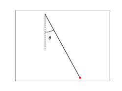
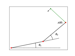
Figure 1: Control settings considered. From left to right: pendulum, two-link arm robot.

Pendulum.

We consider a simple pendulum illustrated in Fig. 1, where $m=1$ denotes the mass of the bob, $l=1$ denotes the length of the rod, $\theta$ describes the angle subtended by the vertical axis and the rod, and $\mu=0.01$ is the friction coefficient. The dynamics are described by

$$\ddot{\theta}(t)=-\frac{g}{l}\sin\theta(t)-\frac{\mu}{ml^{2}}\dot{\theta}(t)+\frac{1}{ml^{2}}u(t)$$

The goal is to make the pendulum swing up (i.e. make an angle of $\pi$ radians) and stop at a given time $T$. The cost writes as

$$J(x,u)=(\pi-x_{1}(T))^{2}+\lambda_{1}x_{2}(T)^{2}+\lambda_{2}\int_{0}^{T}u^{2}(t)dt,$$ (46)

where $x(t)=(\theta(t),\dot{\theta}(t))$, $\lambda_{1}=0.1,\lambda_{2}=0.01$, $T=5$.

Two-link arm.

We consider the arm model with two joints (shoulder and elbow), moving in the horizontal plane presented in (Li & Todorov, 2004) and illustrated in 1. The dynamics are described by

$$M(\theta(t))\ddot{\theta}(t)+C(\theta(t),\dot{\theta}(t))+B\dot{\theta}(t)=u(t),$$ (47)

where $\theta=(\theta_{1},\theta_{2})$ is the joint angle vector, $M(\theta)\in{\mathbb{R}}^{2\times 2}$ is a positive definite symmetric inertia matrix, $C(\theta,\dot{\theta})\in{\mathbb{R}}^{2}$ is a vector centripetal and Coriolis forces, $B\in{\mathbb{R}}^{2\times 2}$ is the joint friction matrix, and $u(t)\in{\mathbb{R}}^{2}$ is the joint torque that we control. We drop the dependence on $t$ for readability. The dynamics are then

$$\ddot{\theta}=M(\theta)^{-1}(u-C(\theta,\dot{\theta})-B\dot{\theta}).$$ (48)

The expressions of the different variables and parameters are given by

$$M(\theta) =\left(\begin{matrix}a_{1}+2a_{2}\cos\theta_{2}&a_{3}+a_{2}\cos\theta_{2}\\ a_{3}+a_{2}\cos\theta_{2}&a_{3}\end{matrix}\right) C(\theta,\dot{\theta}) =\left(\begin{matrix}-\dot{\theta}_{2}(2\dot{\theta}_{1}+\dot{\theta}_{2})\\ \dot{\theta}_{1}^{2}\end{matrix}\right)a_{2}\sin\theta_{2}$$ (49)

$$B =\left(\begin{matrix}b_{11}&b_{12}\\ b_{21}&b_{22}\end{matrix}\right) \begin{array}[]{ll}a_{1}&=k_{1}+k_{2}+m_{2}l_{1}^{2}\\ a_{2}&=m_{2}l_{1}d_{2}\\ a_{3}&=k_{2},\end{array}$$ (53)

where $b_{11}=b_{22}=0.05$, $b_{12}=b_{21}=0.025$, $l_{i}$ and $k_{i}$ are respectively the length (30cm, 33cm) and the moment of inertia (0.025kgm² , 0.045kgm²) of link $i$ , $m_{2}$ and $d_{2}$ are respectively the mass (1kg) and the distance (16cm) from the joint center to the center of the mass for the second link.

The goal is to make the arm reach a feasible target $\theta^{*}$ and stop at that point. The objective reads

$$J(x,u)=\|\theta(T)-\theta^{*}\|^{2}+\lambda_{1}\|\dot{\theta}(T)\|^{2}+\lambda_{2}\int_{0}^{T}\|u(t)\|^{2}dt,$$ (54)

where $x(t)=(\theta(t),\dot{\theta}(t))$, $\lambda_{1}=0.1,\lambda_{2}=0.01$, $T=5$.

5.2 Results

We use the automatic differentiation capabilities of PyTorch (Paszke et al., 2017) to implement the automatic differentiation oracles introduced in Sec. 3. The Gauss-Newton-type steps in Algo. 1 are computed by solving the dual problem associated as presented in Sec. 3.

In Figure 2, we compare the convergence, in terms of function value and gradient norm, of ILQR (based on Gauss-Newton), regularized ILQR (based on regularized Gauss-Newton), and accelerated regularized ILQR (based on accelerated regularized Gauss-Newton). These algorithms were presented in Sec. 4.

For ILQR, we use an Armijo line-search to compute the next step. For both the regularized ILQR and the accelerated regularized ILQR, we use a constant step-size sequence tuned after a burn-in phase of 5 iterations. We leave the exploration of more sophisticated line-search strategies for future work.

The plots show stable convergence of the regularized ILQR on these problems. The proposed accelerated regularized Gauss-Newton algorithm displays stable and fast convergence. Applications of accelerated regularized Gauss-Newton algorithms to reinforcement learning problems would be interesting to explore (Recht, 2018; Fazel et al., 2018; Dean et al., 2018).

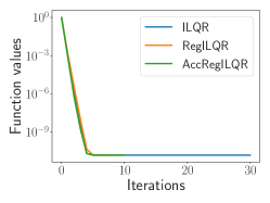
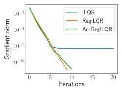
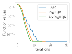
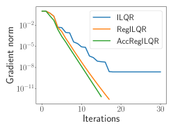
Figure 2: Convergence of ILQR, regularized ILQR and accelerated regularized ILQR on the inverted pendulum (top) and two-link arm (bottom) control problems for an horizon $\tau=100$.

Appendix A Notations

We use semicolons to denote concatenation of vectors, namely for $\tau$ $d$-dimensional vectors $a_{1},\ldots,a_{\tau}\in{\mathbb{R}}^{d}$, we have $(a_{1};\ldots;a_{\tau})\in{\mathbb{R}}^{\tau d}$. The Kronecker product is denoted $\otimes$.

A.1 Tensors

A tensor $\mathcal{A}=(a_{i,j,k})_{i\in\{1,\ldots,d\},j\in\{1,\ldots,n\},k\in\{1,\ldots,p\}}\in{\mathbb{R}}^{d\times n\times p}$ is represented as list of matrices $\mathcal{A}=(A_{1},\ldots,A_{p})$ where $A_{k}=(a_{i,j,k})_{i\in\{1,\ldots,d\},j\in\{1,\ldots,n\}}\in{\mathbb{R}}^{d\times n}$ for $k\in\{1,\ldots p\}$. Given matrices $P\in{\mathbb{R}}^{d\times d^{\prime}},Q\in{\mathbb{R}}^{n\times n^{\prime}},R\in{\mathbb{R}}^{p\times p^{\prime}}$, we denote

$$\mathcal{A}[P,Q,R]=\left(\sum_{k=1}^{p}R_{k,1}P^{\top}A_{k}Q,\ldots,\sum_{k=1}^{p}R_{k,p^{\prime}}P^{\top}A_{k}Q\right)\in{\mathbb{R}}^{d^{\prime}\times n^{\prime}\times p^{\prime}}$$

If $P,Q$ or $R$ are identity matrices, we use the symbol ”$\>\cdot\>$” in place of the identity matrix. For example, we denote $\mathcal{A}[P,Q,\operatorname{I}_{p}]=\mathcal{A}[P,Q,\cdot]=\left(P^{\top}A_{1}Q,\ldots,P^{\top}A_{p}Q\right)$. If $P,Q$ or $R$ are vectors we consider the flatten object. In particular, for $x\in{\mathbb{R}}^{d},y\in{\mathbb{R}}^{n}$, we denote

$$\mathcal{A}[x,y,\cdot]=\left(\begin{matrix}x^{\top}A_{1}y\\ \vdots\\ x^{\top}A_{p}y\end{matrix}\right)\in{\mathbb{R}}^{p}$$

rather than having $\mathcal{A}[x,y,\cdot]\in{\mathbb{R}}^{1\times 1\times p}$. Similarly, for $z\in{\mathbb{R}}^{p}$, we have

$$\mathcal{A}[\cdot,\cdot,z]=\sum_{k=1}^{p}z_{k}A_{k}\in{\mathbb{R}}^{d\times n}.$$

Finally note that we have for $x\in{\mathbb{R}}^{d},y\in{\mathbb{R}}^{n}$ and $R\in{\mathbb{R}}^{p\times p^{\prime}}$,

$$\mathcal{A}(x,y,R)=\left(\sum_{k=1}^{p}x^{\top}A_{k}yR_{k,1},\ldots,\sum_{k=1}^{p}x^{\top}A_{k}yR_{k,p^{\prime}}\right)^{\top}=R^{\top}\mathcal{A}[x,y,\cdot]\in{\mathbb{R}}^{p^{\prime}}.$$

For a tensor $\mathcal{A}=(a_{i,j,k})_{i\in\{1,\ldots,d\},j\in\{1,\ldots,n\},k\in\{1,\ldots,p\}}\in{\mathbb{R}}^{d\times n\times p}$, we denote

$$\mathcal{A}^{\pi}=(a_{k,i,j})_{k\in\{1,\ldots,p\},i\in\{1,\ldots,d\},j\in\{1,\ldots,n\}}\in{\mathbb{R}}^{p\times d\times n}.$$

the tensor whose indexes have been shifted onward. We then have for matrices $P\in{\mathbb{R}}^{d\times d^{\prime}},Q\in{\mathbb{R}}^{n\times n^{\prime}},R\in{\mathbb{R}}^{p\times p^{\prime}}$,

$$(\mathcal{A}[P,Q,R])^{\pi}=\mathcal{A}^{\pi}[R,P,Q].$$

For matrices, we have $A^{\pi}=A^{\top}$ and for one dimensional vectors $x^{\pi}=x$.

A.2 Gradients

Given a state space of dimension $d$, and control space of dimension $p$, for a real function of state and control $f:{\mathbb{R}}^{d+p}\mapsto{\mathbb{R}}$, whose value is denoted $f(x,u)$, we decompose its gradient $\nabla f(x,u)\in{\mathbb{R}}^{d+p}$ on $(x,u)$ as a part depending on the state variables and a part depending on the control variables as follows

$$\nabla f(x,u)=\left(\begin{matrix}\nabla_{x}f(x,u)\\ \nabla_{u}f(x,u)\end{matrix}\right)\qquad\mbox{with}\qquad\nabla_{x}f(x,u)\in{\mathbb{R}}^{d},\quad\nabla_{u}f(x,u)\in{\mathbb{R}}^{p}.$$

Similarly we decompose its Hessian $\nabla f(x,u)\in{\mathbb{R}}^{(d+p)\times(d+p)}$ on blocks that correspond to the state and control variables as follows

$$\nabla^{2}f(x,u)=\left(\begin{matrix}\nabla_{xx}f(x,u)&\nabla_{xu}f(x,u)\\ \nabla_{ux}f(x,u)&\nabla_{uu}f(x,u)\end{matrix}\right)$$

$$\qquad\mbox{with}\qquad\nabla_{xx}f(x,u)\in{\mathbb{R}}^{d\times d},\quad\nabla_{uu}f(x,u)\in{\mathbb{R}}^{p\times p},\nabla_{xu}f(x,u)=\nabla_{ux}f(x,u)^{\top}\in{\mathbb{R}}^{d\times p}.$$

For a multivariate function $f:{\mathbb{R}}^{d}\mapsto{\mathbb{R}}^{n}$, composed of $f^{(j)}$ real functions with $j\in\{1,\ldots n\}$, we denote $\nabla f(x)=(\nabla f^{(1)}(x),\ldots,\nabla f^{(n)}(x))\in{\mathbb{R}}^{d\times n}$, that is the transpose of its Jacobian on $x$, $\nabla f(x)=(\frac{\partial f^{(j)}}{\partial x_{i}}(x))_{\begin{subarray}{c}1\leq i\leq d,1\leq j\leq n\end{subarray}}\in{\mathbb{R}}^{d\times n}$. We represent its second order information by a tensor $\nabla^{2}f(x)=(\nabla^{2}f^{(1)}(x),\ldots,\nabla^{2}f^{(n)}(x))\in{\mathbb{R}}^{d\times d\times n}$

We combine previous definitions to describe the dynamic functions. Given a state space of dimension $d$, a control space of dimension $p$ and an output space of dimension $d_{+}$, for a dynamic function $\phi:{\mathbb{R}}^{d+p}\mapsto{\mathbb{R}}^{d_{+}}$ and a pair of control and state variable $(x,u)$, we denote $\nabla_{x}\phi(x,u)=(\nabla_{x}\phi^{(1)}(x,u),\ldots,\nabla_{x}\phi^{(d_{+})}(x,u))$ and we define similarly $\nabla_{u}\phi(x,u)$. For its second order information we define $\nabla_{xx}\phi(x,u)=(\nabla_{xx}\phi^{(1)}(x,u),\ldots,\nabla_{xx}\phi^{(d_{+})}(x,u))$, similarly for $\nabla_{xx}\phi(x,u)$. Dimension of these definitions are

$$\nabla_{x}\phi(x,u)\in{\mathbb{R}}^{d\times d_{+}},\quad\nabla_{u}\phi(x,u)\in{\mathbb{R}}^{p\times d_{+}},\nabla_{xx}\phi(x,u)\in{\mathbb{R}}^{d\times d\times d_{+}},\quad\nabla_{uu}\phi(x,u)\in{\mathbb{R}}^{p\times p\times d_{+}}$$

$$\nabla_{xu}\phi(x,u)\in{\mathbb{R}}^{d\times p\times d_{+}},\quad\nabla_{ux}\phi(x,u)\in{\mathbb{R}}^{p\times d\times d_{+}}.$$

Appendix B Dynamic programming for linear quadratic optimal control problems

We present the dynamic programming resolution of the Linear Quadratic control problem

$$\begin{split}\underset{\begin{subarray}{c}x_{0},\ldots,x_{\tau}\in{\mathbb{R}}^{d}\\ u_{0},\ldots,u_{\tau-1}\in{\mathbb{R}}^{p}\end{subarray}}{\mbox{min}}\quad&\sum_{t=1}^{\tau}h_{t}(x_{t})+\sum_{t=0}^{\tau-1}g_{t}(u_{t})\\ \mbox{subject to}\quad&x_{t+1}=\phi_{t}(x_{t},u_{t})\qquad\mbox{for $t=0,\ldots,\tau-1$}\\ &x_{0}\quad=\hat{x}_{0},\end{split}$$ (55)

with

$$\phi(x,u)=\Phi_{t,x}^{\top}x+\Phi_{t,u}^{\top}u,\qquad h_{t}(x)=h_{t,x}^{\top}x+\frac{1}{2}x^{\top}H_{t,xx},\quad\mbox{and}\quad g_{t}(u)=g_{t,u}^{\top}u+\frac{1}{2}u^{\top}G_{t,uu}u,$$

where $\Phi_{t,x}\in{\mathbb{R}}^{d\times d},\Phi_{t,u}\in{\mathbb{R}}^{p\times d}$, $h_{t,x}\in{\mathbb{R}}^{d},g_{t,u}\in{\mathbb{R}}^{p},H_{t,xx}\in{\mathbb{R}}^{d\times d},G_{t,uu}\in{\mathbb{R}}^{p\times p}$ with $H_{t,xx}\succeq 0$ and $G_{t,uu}\succ 0$.

Dynamic programming applied to this problem is presented in Algo. 2 it is based on the following proposition that computes cost-to-go functions as quadratics.

Proposition B.1.

Cost-to-go functions (20) to minimize are quadratics of the form, for $t\in{0,\ldots,\tau}$,

$$c_{t}(x)=\frac{1}{2}x^{\top}C_{t,xx}x+c_{t,x}^{\top}x,\quad\mbox{with $C_{t,xx}\succeq 0$}. \mathcal{H}_{t}$$ ()

The optimal control at time $t$ from a state $x_{t}$ reads for $t\in\{0,\ldots,\tau-1\}$,

$$u^{*}_{t}(x_{t})=K_{t}x_{t}+k_{t}$$

where $C_{t,xx},c_{t,x},K_{t},k_{t}$ are defined recursively in lines 5, 7, 8, 9 of Algo. 2.

Proof.

We prove recursively ($\mathcal{H}_{t}$). By definition of the cost-to-function, we have

$$c_{\tau}(x) =h_{\tau}(x),\quad\mbox{so}\quad C_{\tau,xx}=H_{\tau,xx},\quad c_{\tau,x}=h_{\tau,x},$$

and by assumption on the costs $C_{\tau,xx}=H_{\tau,xx}\succeq 0$, which ensures $(\mathcal{H}_{\tau})$.

Then for $0\leq t\leq\tau-1$, assume $(\mathcal{H}_{t+1})$, we search to compute

$$c_{t}(x)=h_{t}(x)+\min_{u}\{g_{t}(u)+c_{t+1}(\phi_{t}(x,u))\}$$

To follow the computations, we drop the dependency on time and denote by superscript ^′ the quantities at time $t+1$, e.g. $c^{\prime}=c_{t+1}$. We therefore search an expression for

$$c(x)=h(x)+\min_{u}\{g(u)+c^{\prime}(\phi(x,u))\}=\min_{u}W(x,u).$$ (56)

The function $W$ is a quadratic in $(x,u)$ of the form

$$W(x,u)=w_{x}^{\top}x+w_{u}^{\top}u+\frac{1}{2}x^{\top}W_{xx}x+\frac{1}{2}u^{\top}W_{uu}u+u^{\top}W_{ux}x.$$

Developing the terms in (56) we have

$$W(x,u) =h_{x}^{\top}x+g_{u}^{\top}u+\frac{1}{2}x^{\top}H_{xx}x+\frac{1}{2}u^{\top}G_{uu}u$$

$$+\frac{1}{2}(\Phi_{x}^{\top}x+\Phi_{u}^{\top}u)^{\top}C^{\prime}_{xx}(\Phi_{x}^{\top}x+\Phi_{u}^{\top}u)+(\Phi_{x}^{\top}x+\Phi_{u}^{\top}u)^{\top}c^{\prime}_{x}.$$

By identification and using that $C^{\prime}_{xx}$ is symmetric, we get

$$w_{x} =g_{x}+\Phi_{x}c^{\prime}_{x} W_{xx} =H_{xx}+\Phi_{x}C^{\prime}_{xx}\Phi_{x}^{\top}$$

$$w_{u} =g_{u}+\Phi_{u}c^{\prime}_{x} W_{uu} =G_{uu}+\Phi_{u}C^{\prime}_{xx}\Phi_{u}^{\top}$$

$$W_{ux} =\Phi_{u}C^{\prime}_{xx}\Phi_{x}^{\top}.$$

By assumption $G_{uu}\succ 0$ and by $(H_{t+1})$, $C^{\prime}_{xx}\succeq 0$, therefore $W_{uu}\succ 0$, minimization in $u$ in (56) is possible and reads

$$c(x) =w_{x}^{\top}x+\frac{1}{2}x^{\top}W_{xx}x-\frac{1}{2}(W_{ux}x+w_{u})^{\top}W_{uu}^{-1}(W_{ux}x+w_{u}),$$

with optimal control variable

$$u^{*}(x)=-W_{uu}^{-1}(W_{ux}x+w_{u}).$$

Cost-to-go $c$ is then defined by (ignoring the constant terms for the minimization)

$$c_{x} =w_{x}-W_{ux}^{\top}W_{uu}^{-1}w_{u}$$

$$C_{xx} =W_{xx}-W_{ux}^{\top}W_{uu}^{-1}W_{ux}.$$

Denote then $C_{xx}^{{}^{\prime}1/2}$ a squared root matrix of $C^{\prime}_{xx}\succeq 0$ such that $(C_{xx}^{{}^{\prime}1/2})^{\top}C_{xx}^{{}^{\prime}1/2}=C^{\prime}_{xx}$. Developing the terms in the last equation gives

$$C_{xx} =W_{xx}-W_{ux}^{\top}W_{uu}^{-1}W_{ux}$$

$$=H_{xx}+\Phi_{x}C^{\prime}_{xx}\Phi_{x}^{\top}-\Phi_{x}C^{\prime}_{xx}\Phi_{u}^{\top}(G_{uu}+\Phi_{u}C^{\prime}_{xx}\Phi_{u}^{\top})^{-1}\Phi_{u}C^{\prime}_{xx}\Phi_{x}^{\top}$$

$$=H_{xx}+\Phi_{x}C_{xx}^{{}^{\prime}1/2\top}\left(I-C_{xx}^{{}^{\prime}1/2}\Phi_{u}^{\top}(G_{uu}+\Phi_{u}C_{xx}^{{}^{\prime}}\Phi_{u}^{\top})^{-1}\Phi_{u}C_{xx}^{{}^{\prime}1/2\top}\right)C_{xx}^{{}^{\prime}1/2}\Phi_{x}^{\top}$$

$$=H_{xx}+\Phi_{x}C_{xx}^{{}^{\prime}1/2\top}\left(I+C_{xx}^{{}^{\prime}1/2}\Phi_{u}^{\top}G_{uu}^{-1}\Phi_{u}C_{xx}^{{}^{\prime}1/2\top}\right)^{-1}C_{xx}^{{}^{\prime}1/2}\Phi_{x}^{\top}\succeq 0,$$

where we used Sherman-Morrison-Woodbury’s formula in the last equality. This therefore proves $(\mathcal{H}_{t})$ and the recurrence. ∎

Algorithm 2 Dynamic Programming for Linear Dynamics, Quadratic Convex Costs (55)

1:Initial state $\hat{x}_{0}$,

2:Quadratic costs defined by $h_{t,x},H_{t,xx}$ with $H_{t,xx}\succeq 0$ for $t=1,\ldots,\tau$ and $g_{t,u},G_{t,uu}$ with $G_{t,uu}\succ 0$, for $t=0,\ldots,\tau-1$

3:Linear dynamics defined by $\Phi_{t,x},\Phi_{t,u}$ for $t=0,\ldots,\tau-1$

4:Backward pass

5:Initialize $C_{\tau,xx}=H_{\tau,xx},c_{\tau,x}=h_{\tau,x}$

6:for $t=\tau-1,\ldots,0$  do

7:      Define

$$w_{t,x} =h_{t,x}+\Phi_{t,x}c_{t+1,x} W_{t,xx} =H_{t,xx}+\Phi_{t,x}C_{t+1,xx}\Phi_{t,x}^{\top}$$

$$w_{t,u} =g_{t,u}+\Phi_{t,u}c_{t+1,u} W_{t,uu} =G_{t,uu}+\Phi_{t,u}C_{t+1,xx}\Phi_{t,u}^{\top}$$

$$W_{t,ux} =\Phi_{t,u}C_{t+1,xx}\Phi_{t,x}^{\top}$$

8:     Compute

$$C_{t,xx}=W_{t,xx}-W_{t,ux}^{\top}W_{t,uu}^{-1}W_{t,ux}\qquad\qquad c_{t,x}=w_{t,x}-W_{t,ux}^{\top}W_{t,uu}^{-1}w_{t,u}$$

9:     Store

$$K_{t}=-W_{t,uu}^{-1}W_{t,ux}\qquad\qquad k_{t}=-W_{t,uu}^{-1}w_{t,u}$$

10:end for

11:Roll-out pass

12:Initialize $x_{0}=\hat{x}_{0}$

13:for $t=0,\ldots,\tau-1$ do

$$u_{t}^{*}=K_{t}x_{t}+k_{t}\qquad\qquad x_{t+1}=\Phi_{t,x}^{\top}x_{t}+\Phi_{t,u}^{\top}u_{t}^{*}$$

14:end for

15:Optimal $u_{0}^{*},\ldots,u_{\tau-1}^{*}$ for (55)

Appendix C Control algorithms detailed

We detail the complete implementation of the control algorithms presented in Section 4. We detail the simple implementations of ILQR (Li & Todorov, 2004), ILQG (Todorov & Li, 2005; Li & Todorov, 2007), the variant of ILQG (Tassa et al., 2012) and DDP (Mayne, 1966). Various line-searches have been proposed as in e.g. (Tassa et al., 2012). We leave their analysis for future work.

C.1 ILQR (Li & Todorov, 2004) and regularized ILQR

ILQR and regularized ILQR amount to solve

$$\min_{\begin{subarray}{c}y_{0},\ldots y_{\tau}\in{\mathbb{R}}^{d}\\ v_{0},\ldots,v_{\tau-1}\in{\mathbb{R}}^{p}\end{subarray}} \sum_{t=1}^{\tau}q_{h_{t}}(x_{t}+y_{t};x_{t})+\sum_{t=0}^{\tau-1}q_{g_{t}}(u_{t}+v_{t};u_{t})+{\color[rgb]{0.80,0.20,0}\frac{1}{\bm{2\gamma}}\|\bm{v_{t}}\|_{2}^{2}}$$ (57)

subject to $$y_{t+1}=\Phi_{t,x}^{\top}y_{t}+\Phi_{t,u}^{\top}v_{t}$$

$$y_{0}=0,$$

where $\Phi_{t,x}=\nabla_{x}\phi_{t}(x_{t},u_{t})$, $\Phi_{t,u}=\nabla_{u}\phi_{t}(x_{t},u_{t})$, $x_{t}=\tilde{x}_{t}(\bar{u})$ and

$$q_{h_{t}}(x_{t}+y_{t};x_{t}) =h_{t}(x_{t})+h_{t,x}^{\top}y_{t}+\frac{1}{2}y_{t}^{\top}H_{t,xx}y_{t}$$

$$q_{g_{t}}(u_{t}+v_{t};u_{t}) =g_{t}(u_{t})+g_{t,u}^{\top}v_{t}+\frac{1}{2}v_{t}^{\top}G_{t,uu}v_{t},$$

where $h_{t,x}=\nabla h_{t}(x_{t})$, $H_{t,xx}=\nabla^{2}h_{t}(x_{t})\succeq 0$, $g_{t,u}=\nabla g_{t}(u_{t})$, $G_{t,uu}=\nabla^{2}g_{t}(u_{t})\succeq 0$.

For ${\color[rgb]{0.80,0.20,0}\bf\bm{\gamma}}=+\infty$, this amounts to the ILQR method. If $h$, $g$ are quadratics this is a Gauss-Newton step, otherwise it amounts to a generalized Gauss-Newton step. For ${\color[rgb]{0.80,0.20,0}\bf\bm{\gamma}}<+\infty$, if $h$, $g$ are quadratics this amounts to a regularized Gauss-Newton step (14), otherwise it amounts to a Levenberg-Marquardt step (16).

The steps (57) are detailed in Algo. 3 based on the derivations made in Section B. The complete methods are detailed in Algo. 7 for the ILQR algorithm and in Algo. 8 for the regularized step. For the classical ILQR method, an Armijo line-search can be used to ensure decrease of the objective as we present in Algorithm 7. Different line-searches were proposed, like the one used in Differential dynamic Programming (see below). A line-search for the regularized ILQR is proposed in Algo. 14 based on the regularized Gauss-Newton method’s analysis. Note that theoretically a constant step-size can also be used a shown in Sec. 4. More sophisticated line-searches with proven convergence rates are left for future work. Note that they were experimented in (Li & Todorov, 2007) for the ILQG method.

C.2 ILQG (Todorov & Li, 2005; Li & Todorov, 2007) and regularized ILQG

The ILQG method as presented in (Todorov & Li, 2005; Li & Todorov, 2007) consists in approximating the linearized trajectory by a Gaussian as presented in Sec. 2 and solve the corresponding dynamic programming. As for ILQR we add a proximal term to account for the inaccuracy of the model. Formally it amounts to solve

$$\min_{\begin{subarray}{c}y_{0},\ldots y_{\tau}\in{\mathbb{R}}^{d}\\ v_{0},\ldots,v_{\tau-1}\in{\mathbb{R}}^{p}\end{subarray}}\quad\sum_{t=1}^{\tau}\operatorname{\mathbb{E}}_{\bar{w}}\left[q_{h_{t}}(x_{t}+y_{t};x_{t})\right]+\sum_{t=0}^{\tau-1}q_{g_{t}}(u_{t}+v_{t};u_{t})+{\color[rgb]{0.80,0.20,0}\frac{1}{\bm{2\gamma}}\|\bm{v_{t}}\|_{2}^{2}}$$ (58)

$$\mbox{{s.t.}}\quad y_{t+1}=\Phi_{t,x}^{\top}y_{t}+\Phi_{t,u}^{\top}v_{t}+\Phi_{t,w}^{\top}w_{t}+\upphi_{t,u,w}[v_{t},w_{t},\cdot],$$

$$\phantom{\mbox{{s.t}}\quad\quad\>}y_{0}=0,$$

where $\Phi_{t,x}=\nabla_{x}\phi_{t}(x_{t},u_{t},0)$, $\Phi_{t,u}=\nabla_{u}\phi_{t}(x_{t},u_{t},0)$, $\Phi_{t,w}=\nabla_{w}\phi_{t}(x_{t},u_{t},0)$, $\upphi_{t,u,w}=\nabla_{uw}^{2}\phi_{t}(x_{t},u_{t},0)$, $x_{t}=\tilde{x}_{t}(\bar{u},0)$, and

$$q_{h_{t}}(x_{t}+y_{t};x_{t}) =h_{t}(x_{t})+h_{t,x}^{\top}y_{t}+\frac{1}{2}y_{t}^{\top}H_{t,xx}y_{t}$$

$$q_{g_{t}}(u_{t}+v_{t};u_{t}) =g_{t}(u_{t})+g_{t,u}^{\top}v_{t}+\frac{1}{2}v_{t}^{\top}G_{t,uu}v_{t},$$

where $h_{t,x}=\nabla h_{t}(x_{t})$, $H_{t,xx}=\nabla^{2}h_{t}(x_{t})\succeq 0$, $g_{t,u}=\nabla g_{t}(u_{t})$, $G_{t,uu}=\nabla^{2}g_{t}(u_{t})\succeq 0$.

The classical ILQG algorithm did not take into account a regularization as presented in Algo. 9 where we present an Armijo line-search though other line-searches akin to the ones made for DDP are possible. Its regularized version is presented in Algo. 10. They are based on solving the above problem at each step as presented in Algo. 4. It is based on the following resolution of the dynamic programming problem.

Proposition C.1.

Cost-to-go functions for problem (58) are quadratics of the form, for $t\in{0,\ldots,\tau}$,

$$c_{t}(x)=\frac{1}{2}x^{\top}C_{t,xx}x+c_{t,x}^{\top}x,\quad\mbox{with $C_{t,xx}\succeq 0$}.$$ (59)

The optimal control at time $t$ from a state $x_{t}$ reads for $t\in\{0,\ldots,\tau-1\}$,

$$u^{*}_{t}(x_{t})=K_{t}x_{t}+k_{t}$$

where $C_{t,xx},c_{t,x},K_{t},k_{t}$ are defined recursively in Algo. 4.

Proof.

The classical Bellman equation is replaced for problem (58) by

$$c_{t}(\hat{y}_{t})=q_{h_{t}}(\hat{y}_{t})+\min_{v_{t}}\left\{q_{g_{t}}(v_{t})+\frac{1}{2\gamma}\|v_{t}\|_{2}^{2}+\operatorname{\mathbb{E}}_{w_{t}}\left[c_{t+1}(\Phi_{t,x}^{\top}y_{t}+\Phi_{t,u}^{\top}v_{t}+\Phi_{t,w}^{\top}w_{t}+\upphi_{t,u,w}[v_{t},w_{t},\cdot])\right]\right\}.$$ (60)

where we denoted shortly $q_{h_{t}}(\hat{y}_{t})=q_{h_{t}}(x_{t}+y_{t};x_{t})$ and $q_{g_{t}}(v_{t})=q_{g_{t}}(u_{t}+v_{t};u_{t})$.

The dynamic programming procedure is initialized by $c_{\tau,x}=h_{\tau,x}$, $C_{\tau,xx}=H_{\tau,xx}\succeq 0$. At iteration $t$, we seek to solve analytically the equation (60). For given $y$ and $v$. denoting with ^′ the quantities at time $t+1$ and omitting the index $t$ otherwise, the expectation in (60) reads (recall that we supposed $w_{t}\sim\mathcal{N}(0,\operatorname{I}_{q})$)

$$E= \operatorname{\mathbb{E}}_{w}\left[c^{\prime}(\Phi_{x}^{\top}y+\Phi_{u}^{\top}v+\Phi_{w}^{\top}w+\upphi_{u,w}[v,w,\cdot])\right]$$

$$= \operatorname{\mathbb{E}}_{w}\Big{[}{c_{x}^{\prime}}^{\top}(\Phi_{x}^{\top}y+\Phi_{u}^{\top}v+\Phi_{w}^{\top}w+\upphi_{u,w}[v,w,\cdot])$$

$$\phantom{\operatorname{\mathbb{E}}_{w}\Big{[}}+\frac{1}{2}(\Phi_{x}^{\top}y+\Phi_{u}^{\top}v+\Phi_{w}^{\top}w+\upphi_{u,w}[v,w,\cdot])^{\top}{C^{\prime}}_{xx}(\Phi_{x}^{\top}y+\Phi_{u}^{\top}v+\Phi_{w}^{\top}w+\upphi_{u,w}[v,w,\cdot])\Big{]}$$

$$= {c_{x}^{\prime}}^{\top}(\Phi_{x}^{\top}y+\Phi_{u}^{\top}v)+\frac{1}{2}(\Phi_{x}^{\top}y+\Phi_{u}^{\top}v)^{\top}{C^{\prime}}_{xx}(\Phi_{x}^{\top}y+\Phi_{u}^{\top}v)$$

$$+\operatorname{\mathbb{E}}_{w}\Big{[}\frac{1}{2}(\Phi_{w}^{\top}w+\upphi_{u,w}[v,w,\cdot])^{\top}{C^{\prime}_{xx}}(\Phi_{w}^{\top}w+\upphi_{u,w}[v,w,\cdot])\Big{]}$$

Now we have

$$E^{\prime}= \operatorname{\mathbb{E}}_{w}\Big{[}\frac{1}{2}(\Phi_{w}^{\top}w+\upphi_{u,w}[v,w,\cdot])^{\top}{C^{\prime}_{xx}}(\Phi_{w}^{\top}w+\upphi_{u,w}[v,w,\cdot])\Big{]}$$

$$= \operatorname{\mathbb{E}}_{w}\Big{[}\frac{1}{2}(\Phi_{w}^{\top}w+\upphi_{u,w}^{\pi}[\cdot,v,w])^{\top}{C^{\prime}_{xx}}(\Phi_{w}^{\top}w+\upphi_{u,w}^{\pi}[\cdot,v,w])\Big{]}$$

$$= \operatorname{\mathbb{E}}_{w}\Big{[}\frac{1}{2}w^{\top}(\Phi_{w}^{\top}+\upphi_{u,w}^{\pi}[\cdot,v,\cdot])^{\top}{C^{\prime}_{xx}}(\Phi_{w}^{\top}+\upphi_{u,w}^{\pi}[\cdot,v,\cdot])w\Big{]}$$

$$= \frac{1}{2}\operatorname{\bf Tr}((\Phi_{w}^{\top}+\upphi_{u,w}^{\pi}[\cdot,v,\cdot])^{\top}{C^{\prime}_{xx}}(\Phi_{w}^{\top}+\upphi_{u,w}^{\pi}[\cdot,v,\cdot]))$$

where $\upphi_{u,w}^{\pi}=(\Psi_{1},\ldots,\Psi_{q})\in{\mathbb{R}}^{d\times p\times q}$ denotes the shuffled tensor $\upphi_{u,w}$ as defined in Appendix A. Therefore we have $\upphi_{u,w}^{\pi}[\cdot,v,\cdot]=(\Psi_{1}v,\ldots,\Psi_{q}v)\in{\mathbb{R}}^{d\times q}$. Now denoting $\Phi_{w}^{\top}=(\psi_{1},\ldots,\psi_{q})\in{\mathbb{R}}^{d\times q}$, we have

$$E^{\prime}= \frac{1}{2}\operatorname{\bf Tr}\left(C^{\prime}_{xx}\left(\sum_{i=1}^{q}(\psi_{i}+\Psi_{i}v)(\psi_{i}+\Psi_{i}v)^{\top}\right)\right)=\sum_{i=1}^{q}\frac{1}{2}(\psi_{i}+\Psi_{i}v)^{\top}C^{\prime}_{xx}(\psi_{i}+\Psi_{i}v)=\theta_{0}+v^{\top}\theta+\frac{1}{2}v^{\top}\Theta v$$

where

$$\theta_{0}=\frac{1}{2}\operatorname{\bf Tr}(\Phi_{w}C^{\prime}_{xx}\Phi_{w}^{\top}),\qquad\theta=\sum_{i=1}^{q}\Psi_{i}^{\top}C^{\prime}_{xx}\psi_{i},\qquad\Theta=\sum_{i=1}^{q}\Psi_{i}^{\top}C^{\prime}_{xx}\Psi_{i}\succeq 0.$$

The computation of the cost-to-go function (60) reads then (ignoring the constant terms such as $\theta_{0}$),

$$c(\hat{y})=h_{x}^{\top}y+\frac{1}{2}y^{\top}H_{xx}y+\min_{v}\left\{\tilde{g}_{u}^{\top}v+\frac{1}{2}v^{\top}\tilde{G}_{uu}v+c^{\prime}(\Phi_{x}^{\top}y+\Phi_{u}^{\top}v)\right\}.$$ (61)

where

$$\tilde{g}_{u}=g_{u}+\theta\qquad\tilde{G}_{uu}=G_{uu}+\Theta+\gamma^{-1}\operatorname{I}_{p}$$

The rest of the computations follow form Prop. B.1. The positive semi-definiteness of $C_{xx}$ is ensured since $\Theta\succeq 0$. ∎

C.3 ILQG as in (Tassa et al., 2012)

For completeness, we detail the implementation of ILQG steps as presented in (Tassa et al., 2012) in Algo. 5. The overall method consists in simply iterating these steps, i.e., starting from $\bar{u}_{0}$,

$$\bar{u}_{k+1}=\texttt{iLQG\_step}(\bar{u}_{k}).$$

This algorithm is the same as the Differential Dynamic Programming algorithm (see below) except that second order information of the trajectory is not taken into account. We present a simple line-search as the one used for DDP, although more refined line-searches were proposed in (Tassa et al., 2012).

C.4 Differential Dynamic Programming (Tassa et al., 2014)

For completeness, we present a detailed implementation of Differential Dynamic Programing (DDP) as presented in (Tassa et al., 2014). Note that several variants of the algorithms exist, especially in the implementation of line-searches, see e.g. (De O. Pantoja, 1988). A single step of the differential dynamic programming approach is described in Algo. 6. The overall algorithm simply consists in iterating that step as, starting from $\bar{u}_{0}$,

$$\bar{u}_{k+1}=\texttt{DDP\_step}(\bar{u}_{k}).$$

We present the rationale behind the computations as explained in (Tassa et al., 2014) and precise the discrepancy between the motivation and the implementation. Formally, at a given command $\bar{u}$ with associated trajectory $\bar{x}=\tilde{x}(\bar{u})$, the approach consists in approximating the cost-to-go functions as

$$c_{t}(y)= q_{h_{t}}(x_{t}+y;x_{t})+\min_{v}\left\{q_{g_{t}}(u_{t}+v;u_{t})+q_{c_{t+1}\circ\phi_{t}}(x_{t}+y,u_{t}+v;x_{t},u_{t})\right\},$$ (62)

where for a function $f(y)$, $q_{f}(x+y;x)=f(x)+\nabla f(x)^{\top}y+y^{\top}\nabla^{2}f(x)y/2$ denotes its second order approximation around $x$. They will take the following form, ignoring constant terms for the minimization,

$$c_{t}(y)=\frac{1}{2}y^{\top}C_{t,xx}y+c_{t,x}^{\top}y.$$

The initial value function is an approximation of the last cost around the current point, i.e.

$$c_{\tau}(y)=\frac{1}{2}y^{\top}\nabla^{2}h(x_{\tau})y+\nabla h(x_{\tau})^{\top}y,$$

where we identify $C_{\tau,xx}=\nabla^{2}h(x_{\tau})$, $c_{\tau,x}=\nabla h(x_{\tau})$. At time $t+1$ given an approximate value function $c_{t+1}$, step (62) involves computing a second order approximation around points $(x_{t},u_{t})$ of

$$M_{t+1}(x,u)=h_{t}(x)+g_{t}(u)+c_{t+1}(\phi_{t}(x,u)).$$

Denote $W_{t}(y,v)=q_{M_{t+1}}(x_{t}+y,u_{t}+v;x_{t},u_{t})$. We have, denoting $z=(y;v)\in{\mathbb{R}}^{d+p}$,

$$W_{t}(y,v)= \>q_{M_{t+1}}(x_{t}+y,u_{t}+v;x_{t},u_{t})$$ (63)

$$= \>M_{t+1}(x_{t},u_{t})+\nabla h_{t}(x_{t})^{\top}y+\frac{1}{2}y^{\top}\nabla^{2}h_{t}(x_{t})y+\nabla g_{t}(u_{t})^{\top}v+\frac{1}{2}v^{\top}\nabla^{2}g_{t}(u_{t})v$$

$$\>+\nabla c_{t+1}(\phi_{t}(x_{t},u_{t}))^{\top}\nabla\phi_{t}(x_{t},u_{t})^{\top}z+\frac{1}{2}z^{\top}\nabla\phi_{t}(x_{t},u_{t})\nabla^{2}c_{t+1}(\phi(x_{t},u_{t}))\nabla\phi_{t}(x_{t},u_{t})^{\top}z$$

$$\>+\frac{1}{2}\nabla^{2}\phi(x_{t},u_{t})[z,z,\nabla c_{t+1}(\phi(x_{t},u_{t}))],$$

where $\nabla\phi_{t}(x_{t},u_{t})^{\top}z=(\nabla_{x}\phi_{t}(x_{t},u_{t})^{\top}y+\nabla_{u}\phi_{t}(x_{t},u_{t})^{\top}v)$, and

$$\nabla^{2}\phi(x_{t},u_{t})[z,z,\nabla c_{t+1}(\phi(x_{t},u_{t}))]=\> \nabla_{xx}^{2}\phi(x_{t},u_{t})[y,y,\nabla c_{t+1}(\phi(x_{t},u_{t}))]$$

$$+\nabla_{uu}^{2}\phi(x_{t},u_{t})[v,v,\nabla c_{t+1}(\phi(x_{t},u_{t}))]$$

$$+2\nabla_{ux}^{2}\phi(x_{t},u_{t})[v,y,\nabla c_{t+1}(\phi(x_{t},u_{t}))].$$

By parameterizing $W_{t}(y,v)$ as

$$W_{t}(y,v) =w_{t,0}+w_{t,x}^{\top}y+w_{t,u}^{\top}v+\frac{1}{2}y^{\top}W_{t,xx}y+\frac{1}{2}v^{\top}W_{t,uu}v+v^{\top}W_{t,ux}y,$$

we get after identification

$$\begin{array}[]{l}w_{t,x}=h_{t,x}+\Phi_{t,x}\tilde{c}_{t+1,x}\\ w_{t,u}=g_{t,u}+\Phi_{t,u}\tilde{c}_{t+1,x}\end{array}\qquad\begin{array}[]{l}W_{t,xx}=H_{t,xx}+\Phi_{t,x}C_{t+1,xx}\Phi_{t,x}^{\top}+\upphi_{t,xx}[\cdot,\cdot,\tilde{c}_{t+1,x}]\\ W_{t,ux}=\Phi_{t,u}C_{t+1,xx}\Phi_{t,x}^{\top}+\upphi_{t,ux}[\cdot,\cdot,\tilde{c}_{t+1,x}]\\ W_{t,uu}=G_{t,uu}+\Phi_{t,u}C_{t+1,xx}\Phi_{t,u}^{\top}+\upphi_{t,uu}[\cdot,\cdot,\tilde{c}_{t+1,x}],\end{array}$$

where

$$h_{t,x}=\nabla h_{t}(x_{t}),\qquad H_{t,xx}=\nabla^{2}h_{t}(x_{t}),\qquad g_{t,u}=\nabla g_{t}(u_{t}),\qquad G_{t,uu}=\nabla^{2}g_{t}(u_{t}),$$

$$\Phi_{t,x}=\nabla_{x}\phi_{t}(x_{t},u_{t}),\qquad\Phi_{t,u}=\nabla_{u}\phi_{t}(x_{t},u_{t}),\qquad$$

$$\upphi_{t,xx}=\nabla^{2}_{xx}\phi_{t}(x_{t},u_{t}),\qquad\upphi_{t,uu}=\nabla^{2}_{uu}\phi_{t}(x_{t},u_{t}),\qquad\upphi_{t,ux}=\nabla^{2}_{ux}\phi_{t}(x_{t},u_{t}),\qquad$$

$$\tilde{c}_{t+1,x}=c_{t+1,x}+C_{t+1}\phi_{t}(x_{t},u_{t}).$$

Here rather than using $\tilde{c}_{t+1,x}$ as advocated by the idea of approximating the Bellman equation around the current iterate, the implementation uses $c_{t+1}$. To minimize the resulting function in $v$, one must ensure that $W_{t,uu}$ is invertible. This is done by adding a small regularization $\lambda$ such that $W_{t,uu}:=W_{t,uu}+\lambda\operatorname{I}_{p}\succ 0$ as presented in e.g. (De O. Pantoja, 1988) and further explored in (Tassa et al., 2014).

After minimizing in $v$, we get the new approximate value function to minimize

$$c_{t}(y)=\frac{1}{2}y^{\top}C_{t,xx}y+c_{t,x}^{\top}y,$$

with

$$c_{t,x}=w_{t,x}-W_{t,ux}^{\top}W_{t,uu}^{-1}w_{t,u},\qquad C_{t,xx}=W_{t,xx}-W_{t,ux}^{\top}W_{t,uu}^{-1}W_{t,ux}.$$

Once the cost-to-go functions are computed, the next command is given by the solution of these approximated Bellman equations around the trajectory. Precisely, denote

$$v^{*}(y)=\operatorname*{arg\,min}_{v}\left\{q_{g_{t}}(u_{t}+v;u_{t})+q_{c_{t+1}\circ\phi_{t}}(x_{t}+y,u_{t}+v;x_{t},u_{t})\right\}=K_{t}y+k_{t},$$

where $k_{t}=-W_{t,uu}^{-1}w_{t,u}$ and $K_{t}=-W_{t,uu}^{-1}W_{t,ux}y$. The roll-out phase starts with $x_{0}^{+}=\hat{x}_{0}$ and outputs the next command as

$$u_{t}^{+}=u_{t}+v^{*}(x_{t}^{+}-x_{t})=u_{t}+K_{t}(x_{t}^{+}-x_{t})+k_{t}\qquad x_{t+1}^{+}=\phi_{t}(x_{t}^{+},u_{t}^{+}).$$ (64)

A line-search advocated in e.g. (Tassa et al., 2014) is to move along the direction given by the fixed gain $k_{t}$, i.e., the roll-out phase reads

$$u_{t}^{+}=u_{t}+K_{t}(x_{t}^{+}-x_{t})+\alpha k_{t}\qquad x_{t+1}^{+}=\phi_{t}(x_{t}^{+},u_{t}^{+}),$$

where $\alpha$ is chosen such that the next iterate has a lower cost than the previous one, by a decreasing line-search initialized at $\alpha=1$. More sophisticated line-searches were also proposed (Mayne, 1966; Liao & Shoemaker, 1992).

Algorithm 3 $\texttt{ILQR\_step}(\bar{u},\gamma)$. ILQR step (Li & Todorov, 2004) ($\gamma=\infty$) or regularized ILQR step with step-size $\gamma$ [Sec. 4] on a command $\bar{u}$.

1:Inputs: Command $\bar{u}=(u_{0};\ldots,u_{\tau-1})$, step-size $\gamma$, initial state $\hat{x}_{0}$ convex twice differentiable costs $h_{t}$ for $t=0,\ldots\tau$ with $h_{0}=0$, convex twice differentiable penalties $g_{t}$ for $t=0,\ldots,\tau-1$ differentiable dynamics $\phi_{t}$ for $t=0,\ldots,\tau-1$

2: Forward pass:

3:Set $x_{0}=\hat{x}_{0}$

4:for $t=0,\ldots,\tau-1$ do

5:     Compute and store

$$h_{t,x}=\nabla h_{t}(x_{t}),\quad H_{t,xx}=\nabla^{2}h_{t}(x_{t}),\quad g_{t,u}=\nabla g_{t}(u_{t}),\quad G_{t,uu}=\nabla^{2}g_{t}(u_{t}),$$

$$\Phi_{t,x}=\nabla_{x}\phi_{t}(x_{t},u_{t}),\quad\Phi_{t,u}=\nabla_{u}\phi_{t}(x_{t},u_{t}).$$

6:     Go to next state $x_{t+1}=\phi_{t}(x_{t},u_{t})$

7:end for

8:Backward pass:

9:Initialize $C_{\tau,xx}=\nabla^{2}h_{\tau}(x_{\tau}),c_{\tau,x}=\nabla h_{\tau}(x_{\tau})$

10:for $t=\tau-1,\ldots,0$  do

11:      Define

$$w_{t,x} =h_{t,x}+\Phi_{t,x}c_{t+1,x} W_{t,xx} =H_{t,xx}+\Phi_{t,x}C_{t+1,xx}\Phi_{t,x}^{\top}$$

$$w_{t,u} =g_{t,u}+\Phi_{t,u}c_{t+1,x} W_{t,uu} =G_{t,uu}+\Phi_{t,u}C_{t+1,xx}\Phi_{t,u}^{\top}+{\color[rgb]{0.80,0.20,0}\bf\gamma^{-1}\operatorname{I}_{p}}$$

$$W_{t,ux} =\Phi_{t,u}C_{t+1,xx}\Phi_{t,x}^{\top}$$

12:     Compute

$$C_{t,xx}=W_{t,xx}-W_{t,ux}^{\top}W_{t,uu}^{-1}W_{t,ux}\qquad\qquad c_{t,x}=w_{t,x}-W_{t,ux}^{\top}W_{t,uu}^{-1}w_{t,u}$$

13:     Store

$$K_{t}=-W_{t,uu}^{-1}W_{t,ux}\qquad\qquad k_{t}=-W_{t,uu}^{-1}w_{t,u}$$

14:end for

15:Roll-out pass:

16:Initialize $y_{0}=0$

17:for $t=0,\ldots,\tau-1$ do

$$v_{t}^{*}=K_{t}y_{t}+k_{t}\qquad\qquad y_{t+1}=\Phi_{t,x}^{\top}y_{t}+\Phi_{t,u}^{\top}v_{t}^{*}$$

18:end for

19:$\texttt{ILQR\_step}(\bar{u},\gamma)=\bar{v}^{*}$ where $\bar{v}^{*}=(v_{0}^{*};\ldots;v_{\tau-1}^{*})$ is optimal for (57)

Algorithm 4 $\texttt{ILQG\_step}(\bar{u},\gamma)$. ILQG step (Todorov & Li, 2005; Li & Todorov, 2007) ($\gamma=\infty$) or regularized ILQG step with stepsize $\gamma$ [Sec. 4] on a command $\bar{u}$.

1:Inputs: Command $\bar{u}=(u_{0};\ldots,u_{\tau-1})$, step-size $\gamma$, initial state $\hat{x}_{0}$ convex twice differentiable costs $h_{t}$ for $t=0,\ldots\tau$ with $h_{0}=0$, convex twice differentiable penalties $g_{t}$ for $t=0,\ldots,\tau-1$ twice differentiable noisy dynamics $\phi_{t}$ for $t=0,\ldots,\tau-1$ as in (3).

2: Forward pass:

3:Set $x_{0}=\hat{x}_{0}$

4:for $t=0,\ldots,\tau-1$ do

5:     Compute and store

$$h_{t,x}=\nabla h_{t}(x_{t}),\quad H_{t,xx}=\nabla^{2}h_{t}(x_{t}),\quad g_{t,u}=\nabla g_{t}(u_{t}),\quad G_{t,uu}=\nabla^{2}g_{t}(u_{t}),$$

$$\Phi_{t,x}=\nabla_{x}\phi_{t}(x_{t},u_{t},0),\quad\Phi_{t,u}=\nabla_{u}\phi_{t}(x_{t},u_{t},0),\quad\Phi_{t,w}=\nabla_{w}\phi_{t}(x_{t},u_{t},0),\quad\upphi_{t,u,w}=\nabla_{uw}^{2}\phi_{t}(x_{t},u_{t},0)$$

6:     Go to the exact next state $x_{t+1}=\phi_{t}(x_{t},u_{t},0)$

7:end for

8:Backward pass:

9:Initialize $C_{\tau,xx}=\nabla^{2}h_{\tau}(x_{\tau}),c_{\tau,x}=\nabla h_{\tau}(x_{\tau})$

10:for $t=\tau-1,\ldots,0$  do

11:      Denoting $(\psi_{t,1},\ldots,\psi_{t,q})=\Phi_{t,w}^{\top}$ and $(\Psi_{t,1},\ldots,\Psi_{t,q})=\upphi_{t,u,w}^{\pi}$, define

$$w_{t,x} =h_{t,x}+\Phi_{t,x}c_{t+1,x} W_{t,xx} =H_{t,xx}+\Phi_{t,x}C_{t+1,xx}\Phi_{t,x}^{\top}$$

$$w_{t,u} =g_{t,u}+\Phi_{t,u}c_{t+1,x}+\sum_{i=1}^{q}\Psi_{t,i}^{\top}C_{t+1,xx}\psi_{t,i} W_{t,uu} =G_{t,uu}+\Phi_{t,u}C_{t+1,xx}\Phi_{t,u}^{\top}+\sum_{i=1}^{q}\Psi_{t,i}^{\top}C_{t+1,xx}\Psi_{t,i}+{\color[rgb]{0.80,0.20,0}\bf\gamma^{-1}\operatorname{I}_{p}}$$

$$W_{t,ux} =\Phi_{t,u}C_{t+1,xx}\Phi_{t,x}^{\top}$$

12:     Compute

$$C_{t,xx}=W_{t,xx}-W_{t,ux}^{\top}W_{t,uu}^{-1}W_{t,ux}\qquad\qquad c_{t,x}=w_{t,x}-W_{t,ux}^{\top}W_{t,uu}^{-1}w_{t,u}$$

13:     Store

$$K_{t}=-W_{t,uu}^{-1}W_{t,ux}\qquad\qquad k_{t}=-W_{t,uu}^{-1}w_{t,u}$$

14:end for

15:Roll-out pass:

16:Initialize $y_{0}=0$

17:for $t=0,\ldots,\tau-1$ do

$$v_{t}^{*}=K_{t}y_{t}+k_{t}\qquad\qquad y_{t+1}=\Phi_{t,x}^{\top}y_{t}+\Phi_{t,u}^{\top}v_{t}^{*}$$

18:end for

19:$\texttt{ILQG\_step}(\bar{u},\gamma)=\bar{v}^{*}$ where $\bar{v}^{*}=(v_{0}^{*};\ldots;v_{\tau-1}^{*})$ is optimal for (58)

Algorithm 5 $\texttt{iLQG\_step}(\bar{u})$ iLQG step as presented in (Tassa et al., 2012) on a command $\bar{u}$

1:Command $\bar{u}=(u_{0};\ldots,u_{\tau-1})$, step-size $\gamma$, initial state $\hat{x}_{0}$ convex twice differentiable costs $h_{t}$ for $t=0,\ldots\tau$ with $h_{0}=0$, convex twice differentiable penalties $g_{t}$ for $t=0,\ldots,\tau-1$ differentiable dynamics $\phi_{t}$ for $t=0,\ldots,\tau-1$, decreasing factor $\rho_{-}<1$, control objective $f$

2: Forward pass:

3:Set $x_{0}=\hat{x}_{0}$

4:for $t=0,\ldots,\tau-1$ do

5:     Compute and store

$$h_{t,x}=\nabla h_{t}(x_{t}),\quad H_{t,xx}=\nabla^{2}h_{t}(x_{t}),\quad g_{t,u}=\nabla g_{t}(u_{t}),\quad G_{t,uu}=\nabla^{2}g_{t}(u_{t}),$$

$$\Phi_{t,x}=\nabla_{x}\phi_{t}(x_{t},u_{t}),\quad\Phi_{t,u}=\nabla_{u}\phi_{t}(x_{t},u_{t}).$$

6:     Go to next state $x_{t+1}=\phi_{t}(x_{t},u_{t})$

7:end for

8:Backward pass:

9:Initialize $C_{\tau,xx}=\nabla^{2}h_{\tau}(x_{\tau}),c_{\tau,x}=\nabla h_{\tau}(x_{\tau})$

10:for $t=\tau-1,\ldots,0$  do

11:      Define

$$w_{t,x} =h_{t,x}+\Phi_{t,x}c_{t+1,x} W_{t,xx} =H_{t,xx}+\Phi_{t,x}C_{t+1,xx}\Phi_{t,x}^{\top}$$

$$w_{t,u} =g_{t,u}+\Phi_{t,u}c_{t+1,x} W_{t,uu} =G_{t,uu}+\Phi_{t,u}C_{t+1,xx}\Phi_{t,u}^{\top}$$

$$W_{t,ux} =\Phi_{t,u}C_{t+1,xx}\Phi_{t,x}^{\top}$$

12:     Compute

$$C_{t,xx}=W_{t,xx}-W_{t,ux}^{\top}W_{t,uu}^{-1}W_{t,ux}\qquad\qquad c_{t,x}=w_{t,x}-W_{t,ux}^{\top}W_{t,uu}^{-1}w_{t,u}$$

13:     Store

$$K_{t}=-W_{t,uu}^{-1}W_{t,ux}\qquad\qquad k_{t}=-W_{t,uu}^{-1}w_{t,u}$$

14:end for

15:Roll-out pass:

16:Initialize $x_{0}^{+}=\hat{x}_{0}$, $\alpha=1$

17:repeat

18:     for $t=0,\ldots,\tau-1$ do

$$u_{t}^{+}=u_{t}+K_{t}(x_{t}^{+}-x_{t})+\alpha k_{t}\qquad\qquad{\color[rgb]{0.80,0.20,0}\bm{x_{t+1}^{+}=\phi_{t}(x_{t}^{+},u_{t}^{+})}}$$

19:     end for

20:     Update $\alpha=\rho_{-}\alpha$

21:until $f(\bar{u}^{+})\leq f(\bar{u})$

22:$\texttt{iLQG\_step}(\bar{u})=\bar{u}^{+}$ where $\bar{u}^{+}=(u_{0}^{+};\ldots;u_{\tau-1}^{+})$

Algorithm 6 $\texttt{DDP\_step}(\bar{u})$. Differential dynamic programming step on a command $\bar{u}$ (Tassa et al., 2014)

1:Hyper-parameters: regularization $\lambda_{0}$, increasing regularization factor $\rho^{+}>1$, decreasing factor $\rho_{-}<1$

2:Inputs: Command $\bar{u}=(u_{0};\ldots;u_{\tau-1})$, initial state $\hat{x}_{0}$ convex twice differentiable costs $h_{t}$ for $t=0,\ldots\tau$ with $h_{0}=0$, convex twice differentiable penalties $g_{t}$ for $t=0,\ldots,\tau-1$, twice differentiable dynamics $\phi_{t}$ for $t=0,\ldots,\tau-1$, control objective $f$

3: Forward pass:

4:Set $x_{0}=\hat{x}_{0}$

5:for $t=0,\ldots,\tau$ do

6:     Compute and store

$$h_{t,x}=\nabla h_{t}(x_{t}),\qquad H_{t,xx}=\nabla^{2}h_{t}(x_{t}),\qquad g_{t,u}=\nabla g_{t}(u_{t}),\qquad G_{t,uu}=\nabla^{2}g_{t}(u_{t}),$$

$$\Phi_{t,x}=\nabla_{x}\phi_{t}(x_{t},u_{t}),\qquad\Phi_{t,u}=\nabla_{u}\phi_{t}(x_{t},u_{t}),\qquad$$

$$\upphi_{t,xx}=\nabla^{2}_{xx}\phi_{t}(x_{t},u_{t}),\qquad\upphi_{t,uu}=\nabla^{2}_{uu}\phi_{t}(x_{t},u_{t}),\qquad\upphi_{t,ux}=\nabla^{2}_{ux}\phi_{t}(x_{t},u_{t}).\qquad$$

7:     Go to next state $x_{t+1}=\phi_{t}(x_{t},u_{t})$

8:end for

9:Compute and store $h_{\tau,x}=\nabla h(x_{\tau}),\quad H_{\tau,xx}=\nabla^{2}h(x_{\tau})$

10:Backward pass:

11:Initialize $C_{\tau,xx}=H_{\tau,xx},c_{\tau,x}=h_{\tau,x}$

12:for $t=\tau-1,\ldots,0$  do

13:      Compute

$$\begin{array}[]{l}\\ w_{t,x}=h_{t,x}+\Phi_{t,x}c_{t+1,x}\\ w_{t,u}=g_{t,u}+\Phi_{t,u}c_{t+1,x}\end{array}\qquad\begin{array}[]{l}W_{t,xx}=H_{t,xx}+\Phi_{t,x}C_{t+1,xx}\Phi_{t,x}^{\top}+\upphi_{t,xx}[\cdot,\cdot,c_{t+1,x}]\\ W_{t,ux}=\Phi_{t,u}C_{t+1,xx}\Phi_{t,x}^{\top}+\upphi_{t,ux}[\cdot,\cdot,c_{t+1,x}]\\ W_{t,uu}=G_{t,uu}+\Phi_{t,u}C_{t+1,xx}\Phi_{t,u}^{\top}+\upphi_{t,uu}[\cdot,\cdot,c_{t+1,x}]\end{array}$$ (69)

14:     Set $\lambda=\lambda_{0},\quad W_{t,uu}^{0}=W_{t,uu}$

15:     while $W_{t,uu}\nsucc 0$ do

16:         $W_{t,uu}:=W_{t,uu}^{0}+\lambda\operatorname{I}_{p},\qquad\lambda=\rho^{+}\lambda$

17:     end while

18:     Compute

$$c_{t,x}=w_{t,x}-W_{t,ux}^{\top}W_{t,uu}^{-1}w_{t,u},\quad C_{t,xx}=W_{t,xx}-W_{t,ux}^{\top}W_{t,uu}^{-1}W_{t,ux}.$$

19:     Store $K_{t}=-W_{t,uu}^{-1}W_{t,ux}\quad k_{t}=-W_{t,uu}^{-1}w_{t,u}$.

20:end for

21:Roll-out pass:

22:Initialize $x_{0}^{+}=\hat{x}_{0}$, $\alpha=1$

23:repeat

24:     for $t=0,\ldots,\tau-1$ do

$$u_{t}^{+}=u_{t}+K_{t}(x_{t}^{+}-x_{t})+\alpha k_{t}\qquad\qquad{\color[rgb]{0.80,0.20,0}\bm{x_{t+1}^{+}=\phi_{t}(x_{t}^{+},u_{t}^{+})}}$$

25:     end for

26:     Update $\alpha=\rho_{-}\alpha$

27:until $f(\bar{u}^{+})\leq f(\bar{u})$

28:$\texttt{DDP\_step}(\bar{u})=\bar{u}^{+}$ where $\bar{u}^{+}=(u_{0}^{+};\ldots;u_{\tau-1}^{+})$

Algorithm 7 ILQR (Li & Todorov, 2004)

1:Initial state $\hat{x}_{0}$, differentiable dynamics $\phi_{t}$ for $t=0,\ldots,\tau-1$, convex twice differentiable costs $h_{t}$ for $t=1,\ldots,\tau$, convex twice differentiable penalties $g_{t}$ for $t=0,\ldots,\tau-1$, , total cost $f$ on the trajectory as defined in (10), initial command $\bar{u}_{0}$, number of iterations $K$

2:for $k=0,\ldots,K$ do

3:     Using Algo. 3, compute $\bar{v}_{k}=\texttt{ILQR\_step}(\bar{u}_{k},+\infty)$

4:     Find $\gamma_{k}$ s.t. $f(\bar{u}_{k}+\gamma_{k}\bar{v}_{k})<f(\bar{u}_{k})$

5:     Set $\bar{u}_{k+1}=\bar{u}_{k}+\gamma_{k}\bar{v}_{k}$

6:end for

7:$\bar{u}^{*}=\bar{u}_{K}$

Algorithm 8 Regularized ILQR as presented in Sec. 4

1:Initial state $\hat{x}_{0}$, differentiable dynamics $\phi_{t}$ for $t=0,\ldots,\tau-1$, convex twice differentiable costs $h_{t}$ for $t=1,\ldots,\tau$, convex twice differentiable penalties $g_{t}$ for $t=0,\ldots,\tau-1$, , total cost $f$ on the trajectory as defined in (10), initial command $\bar{u}_{0}$, number of iterations $K$

2:for $k=0,\ldots,K$ do

3:     Find $\gamma_{k}$, such that $\bar{u}_{k+1}=\bar{u}_{k}+\texttt{ILQR\_step}(\bar{u}_{k},\gamma_{k})$ computed by Algo. 3 satisfies

$$f(\bar{u}_{k+1})\leq f(\bar{u}_{k})+\frac{1}{2\gamma_{k}}\|\bar{u}_{k}-\bar{u}_{k+1}\|_{2}^{2}$$

4:end for

5:$\bar{u}^{*}=\bar{u}_{K}$

Algorithm 9 ILQG (Todorov & Li, 2005; Li & Todorov, 2007)

1:Initial state $\hat{x}_{0}$, noisy twice differentiable dynamics $\phi_{t}$ for $t=0,\ldots,\tau-1$, convex twice differentiable costs $h_{t}$ for $t=1,\ldots,\tau$, convex twice differentiable penalties $g_{t}$ for $t=0,\ldots,\tau-1$, , total cost $f$ on the trajectory as defined in (10), initial command $\bar{u}_{0}$, number of iterations $K$

2:for $k=0,\ldots,K$ do

3:     Using Algo. 4, compute $\bar{v}_{k}=\texttt{ILQG\_step}(\bar{u}_{k},+\infty)$

4:     Find $\gamma_{k}$ s.t. $f(\bar{u}_{k}+\gamma_{k}\bar{v}_{k})<f(\bar{u}_{k})$

5:     Set $\bar{u}_{k+1}=\bar{u}_{k}+\gamma_{k}\bar{v}_{k}$

6:end for

7:$\bar{u}^{*}=\bar{u}_{K}$

Algorithm 10 Regularized ILQG as presented in Sec. 4

1:Initial state $\hat{x}_{0}$, differentiable dynamics $\phi_{t}$ for $t=0,\ldots,\tau-1$, convex twice differentiable costs $h_{t}$ for $t=1,\ldots,\tau$, convex twice differentiable penalties $g_{t}$ for $t=0,\ldots,\tau-1$, , total cost $f$ on the trajectory as defined in (10), initial command $\bar{u}_{0}$, number of iterations $K$

2:for $k=0,\ldots,K$ do

3:     Find $\gamma_{k}$, such that $\bar{u}_{k+1}=\bar{u}_{k}+\texttt{ILQG\_step}(\bar{u}_{k},\gamma_{k})$ computed by Algo. 4 satisfies

$$f(\bar{u}_{k+1})\leq f(\bar{u}_{k})+\frac{1}{2\gamma_{k}}\|\bar{u}_{k}-\bar{u}_{k+1}\|_{2}^{2}$$

4:end for

5:$\bar{u}^{*}=\bar{u}_{K}$

Appendix D Differential Dynamic Programming interpretation

A characteristic of Differential Dynamic Programming is that the update pass follows the original trajectory. This little difference makes it very different to the classical optimization schemes we presented so far. Though its convergence is often derived as a Newton’s method, it was shown that in practice it outperforms Newton’s method (Liao & Shoemaker, 1991, 1992). We analyze it as an optimization procedure on the state variables using recursive model-minimization schemes.

D.1 Approximate dynamic programming

We consider problems in the last control variable since any optimal control problem can be written in the form (30) by adding a dimension in the states. We write then Problem (30) as a constrained problem of the form

$$\begin{split}\min_{\begin{subarray}{c}x_{\tau}\in D_{\tau}\end{subarray}}\quad&h_{\tau}(x_{\tau})\end{split}$$ (70)

where the constraint sets $D_{t}$ are defined recursively as

$$D_{0} =\{x_{0}\}$$

$$D_{t+1} =\{x_{t+1}:x_{t+1}=\phi_{t}(x_{t},u_{t}),\>x_{t}\in D_{t}\>,u_{t}\in{\mathbb{R}}^{p}\},\qquad\mbox{for $t=0,\ldots,\tau-1$}.$$

The approximate dynamic approach consists then as a nested sequence of subproblems that attempt to make an approximate step in the space of the last state. Formally, at a given iterate $\hat{x}_{\tau}$ defined by $(\hat{u}_{0},\ldots,\hat{u}_{\tau-1})$, it considers a model-minimization step i.e.

$$\min_{z\in D_{\tau}}V_{\tau}(z):=m_{h_{\tau}}(z;\hat{x}_{\tau})+\gamma^{-1}d(z,\hat{x}_{\tau}),$$ (71)

where $m_{h_{\tau}}(\cdot;\hat{x}_{t})$ is a given model that approximates $h_{\tau}$ around $\hat{x}_{\tau}$, $d(\cdot,\hat{x}_{\tau})$ is a proximal term and $\gamma$ is the step-size of the procedure.

Then the procedure consists in considering recursively model-minimizations steps of functions $V_{t}$, for $t=\tau,\ldots,1$, where each model-minimization step introduces the minimization of a new value function $V_{t}$ on a simpler constraint space.

Formally, assume that at time $t$ the problem considered is

$$\min_{z\in D_{t}}V_{t}(z)$$ (72)

for a given function $V_{t}$ and that one is given an initial point $\hat{z}_{t}\in D_{t}$ with associated sub-command $\hat{v}_{0},\ldots,\hat{v}_{t-1}$ that defines states $\hat{z}_{0},\ldots,\hat{z}_{t}$ as $\hat{z}_{s+1}=\phi_{s}(\hat{z}_{s},\hat{v}_{s})$ for $0\leq s\leq t-1$ with $\hat{z}_{0}=\hat{x}_{0}$. Then developing the constraint set, the problem reads

$$\min_{z\in D_{t-1},v\in{\mathbb{R}}^{p}}M_{t}(z,v):=V_{t}(\phi_{t-1}(z,v))$$ (73)

a minimization step on this problem around the given initial point is

$$\min_{z\in D_{t-1},v\in{\mathbb{R}}^{p}}m_{M_{t}}(z,v;\hat{z}_{t-1},\hat{v}_{t-1})+\gamma^{-1}d((z,v),(\hat{z}_{t-1},\hat{v}_{t-1})).$$ (74)

Then this problem simplifies as

$$\min_{z\in D_{t-1}}V_{t-1}(z):=\min_{v\in{\mathbb{R}}^{p}}m_{M_{t}}(z,v;\hat{z}_{t-1},\hat{v}_{t-1})+\gamma^{-1}d((z,v),(\hat{z}_{t-1},\hat{v}_{t-1})),$$ (75)

which defines the next problem. The initial point of this subproblem is chosen as $\hat{z}_{t-1}$ with associated subcommand $\hat{v}_{0},\ldots,\hat{v}_{t-2}$.

The recursive algorithm is defined in Algo. 11. These use sub-trajectories defined by the dynamics and sub-commands. The way the stopping criterion and the step-sizes are chosen depend on the implementation just as the choices of the model $m$ and the proximal term $d$. The optimal command is tracked along the recursion to be output at the end.

1:Inputs:

2:-Approximate model $m$, proximal term $d$, initial point $\hat{x}_{0}$

3:-Time $t$, value function $V_{t}$

4:-Dynamics $\phi_{0},\ldots,\phi_{t}$, initial point $z_{t}^{0}\in D_{t}$ with associated subcommand $v_{0}^{0},\ldots,v_{t-1}^{0}$ defining states $z_{0}^{0},\ldots,z_{t}^{0}$ as $z_{s+1}^{0}=\phi_{s}(z_{s}^{0},v_{s}^{0})$ for $0\leq s\leq t-1$ with $z_{0}^{0}=\hat{x}_{0}$

5:-Step sizes $(\gamma_{t}^{k})_{k\in\mathbb{N}}$, stopping criterion $\delta_{t}:\mathbb{N}\times{\mathbb{R}}^{d}\rightarrow\{0,1\}$

6:if $t=0$ then

7:     Return $z^{*}=\hat{x}_{0}$

8:else

9:     repeat for $k=1,\ldots$

10:         Denoting $M_{t}(z,v)=V_{t}(\phi_{t-1}(z,v))$ and $\hat{z}=z^{k-1}_{t-1}$, $\hat{v}=v^{k-1}_{t-1}$, define

$$V_{t-1}(z)=\min_{v\in{\mathbb{R}}^{p}}m_{M_{t}}(z,v;\hat{z},\hat{v})+(\gamma_{t}^{k})^{-1}d((z,v),(\hat{z},\hat{v}))$$ (76)

11:          Find $z^{k}_{t-1}$ and its associated subcommand $v_{0}^{k},\ldots,v_{t-2}^{k}$ and subtrajectory $z_{0}^{k},\ldots,z_{t-2}^{k}$ using Algo. 11 s.t.

$$z^{k}_{t-1}\approx\operatorname*{arg\,min}_{y\in D_{t-1}}V_{t-1}(y)$$

fed with

• same $m,d,\hat{x}_{0}$

• time $t-1$, value function $V_{t-1}$

• dynamics $\phi_{0},\ldots,\phi_{t-1}$, initial point $z^{k-1}_{t-1}$ with associated subcommand $v_{0}^{k-1},\ldots,v_{t-2}^{k-1}$

• a strategy of step sizes $(\gamma_{t-1}^{k})_{k\in\mathbb{N}}$ and a stopping criterion $\delta_{t-1}:\mathbb{N}\times{\mathbb{R}}^{d}\rightarrow\{0,1\}$

12:         Compute

$$v^{k}_{t-1}=\operatorname*{arg\,min}_{v\in{\mathbb{R}}^{p}}m_{M_{t}}(z^{k},v;\hat{z},\hat{v})+(\gamma_{t}^{k})^{-1}d((z^{k},v),(\hat{z},\hat{v}))$$ (77)

13:         Compute $z^{k}_{t}=\phi_{t-1}(z^{k}_{t-1},v^{k}_{t-1})$

14:     until stopping criterion $\delta_{t}(k,z^{k}_{t})$ is met

15:     Return $z^{k}_{t}$ with its associated subcommand $v_{0}^{k},\ldots,v_{t-1}^{k}$

16:end if

Algorithm 11 Approximate Dynamic Programming Recursion

The whole procedure instantiates iteratively Algo. 11 on (71) as presented in Algo. 12. Note that it is of potential interest to have a different model-minimization scheme for the outer loop and the inner recursive loop.

Inputs:

-Cost function $h_{\tau}$, outer approximate model $m$, outer proximal term $d$, inner approximate model $\tilde{m}$ and inner proximal term $\tilde{d}$

-Dynamics $\phi_{0},\ldots,\phi_{\tau-1}$, initial point $x_{\tau}^{0}\in D_{\tau}$ with associated command $u_{0}^{0},\ldots,u_{\tau-1}^{0}$ defining states $x_{0}^{0},\ldots,x_{\tau}^{0}$ as $x_{t+1}^{0}=\phi_{t}(x_{t}^{0},u_{t}^{0})$ for $0\leq t\leq\tau-1$ with $x_{0}^{0}=\hat{x}_{0}$

-Step sizes $(\gamma^{k})_{k\in\mathbb{N}}$, stopping criterion $\delta:\mathbb{N}\times{\mathbb{R}}^{d}\rightarrow\{0,1\}$

repeat for $k=1,\ldots$

      Find $x_{\tau}^{k}$ with associated command $u_{0}^{k},\ldots,u_{\tau-1}^{k}$ using Algo. 11 to solve

$$x_{\tau}^{k}\approx\operatorname*{arg\,min}_{z\in D_{\tau}}V_{\tau}(z):=m_{h_{\tau}}(z;x_{\tau}^{k-1})+(\gamma^{k})^{-1}d(z,x_{\tau}^{k-1})$$ (78)

     fed with

• Inner approximate model $\tilde{m}$ and proximal term $\tilde{d}$, initial point $\hat{x}_{0}$

• time $\tau$, value function $V_{\tau}$

• initial point $x_{\tau}^{k-1}$ with associated command $u_{0}^{k-1},\ldots,u_{\tau-1}^{k-1}$

• a strategy of step sizes $(\gamma_{\tau}^{k})_{k\in\mathbb{N}}$ and a stopping criterion $\delta_{\tau}:\mathbb{N}\times{\mathbb{R}}^{d}\rightarrow\{0,1\}$

until Stopping criterion $\delta(k,x^{k}_{\tau})$ is met

$x^{k}_{\tau}$ with associated command $u_{0}^{k},\ldots,u_{\tau-1}^{k}$

Algorithm 12 Approximate Dynamic Programming

D.2 Differential dynamic programming

Differential dynamic programing is an approximate instance of the above algorithm where (i) one considers a second order approximation of the function to define the model $m$, (ii) one does not use a proximal term $d$, (iii) the stopping criterion is simply to stop after one iteration.

Precisely, for a twice differentiable function $f$, on a point $\hat{w}$, we use $m_{f}(w;\hat{w})=q_{f}(w;\hat{w})=f(\hat{w})+\nabla f(\hat{w})^{\top}(w-\hat{w})+\frac{1}{2}(w-\hat{w})^{\top}\nabla^{2}f(\hat{w})(w-\hat{w})$. Notice that without additional assumption on the Hessian $\nabla^{2}f(\hat{w})$, $q_{f}(\cdot;\hat{w})$ may be unbounded below, such that the model-minimization steps may be not well defined. The definition of the models $q_{M_{t}}$ in Eq. (76) correspond to the computations in Eq. (63) that lead to the formulation of the cost-to-go functions $c_{t}$. The solutions output by the recursion in Eq. (77) correspond to the roll-out presented in Eq. (64). Crucially, as in the classical DDP formulation, the output at the $t$^th time step in the roll-out phase (here when the recursion is unrolled line 13 in Algo. 11) is given by the true trajectory.

Recall that the implementation differs from the motivation. The choice of using the un-shifted cost-to-go functions, i.e., choosing $c_{t+1}$ instead of $\tilde{c}_{t+1}$ as presented in Sec. C.4, is not explained by our theoretical approach.

The iLQG method as presented in Tassa et al. (2012) follows the same approach except that they use the quadratic models defined in a Levenberg-Marquardt steps for each model-minimization of the recursion.

Appendix E Regularized Gauss-Newton analysis

For completeness we recall how equality (38) is obtained. As $h,g$ are quadratics, we have $h(\bar{x}+\bar{y})=q_{h}(\bar{x}+\bar{y};\bar{x}),g(\bar{u}+\bar{v})=q_{g}(\bar{u}+\bar{v};\bar{u})$. Therefore $c_{f}(\bar{u}+\bar{v};\bar{u})=q_{f}(\bar{u}+\bar{v};\bar{u})$ with $c_{f}$ defined in (13) and $q_{f}$ defined in (15). The regularized Gauss-Newton step reads then, denoting $\bar{x}_{k}=\tilde{x}(\bar{u}_{k})$, $H=\nabla^{2}h(\bar{x}_{k})$ and $G=\nabla^{2}g(\bar{u}_{k})$

$$\bar{u}_{k+1} =\bar{u}_{k}+\operatorname*{arg\,min}_{\bar{v}}q_{f}(\bar{u}_{k}+\bar{v};\bar{u}_{k})+\frac{1}{2\gamma_{k}}\|\bar{v}\|_{2}^{2}$$

$$=\bar{u}_{k}+\operatorname*{arg\,min}_{\bar{v}}\Big{\{}\nabla h(\bar{x}_{k})^{\top}(\nabla\tilde{x}(\bar{u}_{k})^{\top}\bar{v})+\frac{1}{2}(\nabla\tilde{x}(\bar{u}_{k})^{\top}\bar{v})^{\top}H(\nabla\tilde{x}(\bar{u}_{k})^{\top}\bar{v})$$

$$\phantom{=\bar{u}_{k}+\operatorname*{arg\,min}_{\bar{v}}\Big{\{}}+\nabla g(\bar{u}_{k})^{\top}\bar{v}+\frac{1}{2}\bar{v}^{\top}G\bar{v}+\frac{1}{2\gamma_{k}}\|\bar{v}\|_{2}^{2}\Big{\}}$$

$$=\bar{u}_{k}-(\nabla\tilde{x}({\bar{u}}_{k})H\nabla\tilde{x}({\bar{u}}_{k})^{\top}+G+\gamma_{k}^{-1}\operatorname{I}_{\tau p})^{-1}(\nabla\tilde{x}(\bar{u}_{k})\nabla h(\bar{x}_{k})+\nabla g(\bar{u}_{k}))$$

$$=\bar{u}_{k}-(\nabla\tilde{x}({\bar{u}}_{k})H\nabla\tilde{x}({\bar{u}}_{k})^{\top}+G+\gamma_{k}^{-1}\operatorname{I}_{\tau p})^{-1}\nabla f({\bar{u}}_{k})$$

We prove the overall convergence of the regularized Gauss-Newton method under a sufficient decrease condition. See 4.1

Proof.

For $k\geq 0$,

$$f(\bar{u}_{k})=c_{f}(\bar{u}_{k};\bar{u}_{k}) \stackrel{{\scriptstyle(\star)}}{{\geq}}c_{f}(\bar{u}_{k+1};\bar{u}_{k})+\frac{1}{\gamma_{k}}\|\bar{u}_{k+1}-\bar{u}_{k}\|_{2}^{2}\stackrel{{\scriptstyle\eqref{eq:suff_decrease}}}{{\geq}}f(\bar{u}_{k+1})+\frac{1}{2\gamma_{k}}\|\bar{u}_{k+1}-\bar{u}_{k}\|^{2},$$

where we used in $(\star)$ the definition of $\bar{u}_{k+1}$ and strong convexity of $\bar{u}\rightarrow c(\bar{u};\bar{u}_{k})+(2\gamma_{k})^{-1}\|\bar{u}-\bar{u}_{k}\|_{2}^{2}$. This ensures first that the iterates stay in the initial level set. Then, summing the inequality and taking the minimum gives

$$\min_{k=0,\ldots,N}\gamma_{k}^{-1}\left\|\bar{u}_{k+1}-\bar{u}_{k}\right\|^{2}\leq\frac{2(f(\bar{u}_{0})-f^{*})}{N+1}.$$

Finally using (38), we get

$$\|\nabla f(\bar{u}_{k})\|_{2}\leq(\ell_{\tilde{x},S}^{2}L_{h}+L_{g}+\gamma_{k}^{-1})\|\bar{u}_{k+1}-\bar{u}_{k}\|_{2}.$$

Plugging this in previous inequality and rearranging the terms give the result. ∎

Now we show how the model approximates the objective up to a quadratic error for exact dynamics See 4.2

Proof.

As $\tilde{x}$ has continuous gradients, it is $\ell_{\tilde{x},C}$-Lipschitz continuous and has $L_{\tilde{x},C}$- Lipschitz gradients on $C\subset{\mathbb{R}}^{\tau p}$. Similarly $h$ is $L_{h}$-smooth and $\ell_{h,C^{\prime}}$ on any compact set $C^{\prime}\subset{\mathbb{R}}^{\tau d}$. Now on $C\subset{\mathbb{R}}^{\tau p}$, denote $B\subset{\mathbb{R}}^{\tau p}$ a ball centered at the origin that contains $C$ and $\rho$ its radius. Define $B^{\prime}\subset{\mathbb{R}}^{\tau d}$ a ball centered at the origin of radius $2\rho\ell_{\tilde{x},C}$ and finally $C^{\prime}=\tilde{x}(C)+B^{\prime}$ such that for any $\bar{u},\bar{v}\in C$, $\tilde{x}(\bar{u})+\nabla\tilde{x}(\bar{u})^{\top}(\bar{v}-\bar{u})\in C^{\prime}$. Then for any $\bar{u},\bar{v}\in C$,

$$|f(\bar{v})-c_{f}(\bar{v};\bar{u})| =|h(\tilde{x}(\bar{v}))-h\left(\tilde{x}(\bar{u})+\nabla\tilde{x}(\bar{u})^{\top}(\bar{v}-\bar{u})\right)|$$

$$\leq\ell_{h,C^{\prime}}\|\tilde{x}(\bar{v})-\tilde{x}(\bar{u})-\nabla\tilde{x}(\bar{u})^{\top}(\bar{v}-\bar{u})\|_{2}$$

$$\leq\frac{\ell_{h,C^{\prime}}L_{\tilde{x},C}}{2}\|\bar{v}-\bar{u}\|_{2}^{2}$$

where the last line uses $\tilde{x}(\bar{v})=\tilde{x}(\bar{u})+\int_{0}^{1}\nabla\tilde{x}(\bar{u}+s(\bar{v}-\bar{u}))^{\top}(\bar{v}-\bar{u})ds$ and the smoothness of $\tilde{x}$ on $C$. ∎

Finally we precise a minimal step-size for which the sufficient decrease condition is ensured. See 4.3

Proof.

Using (38),

$$\|\bar{u}_{k+1}-\bar{u}_{k}\|_{2}\leq\gamma_{k}\|\nabla f(\bar{u}_{k})\|_{2}$$

so for $\gamma_{k}\leq\ell_{f,S}^{-1}$, $\|\bar{u}_{k+1}-\bar{u}_{k}\|_{2}\leq 1$ and $\bar{u}_{k+1}\in C$. As $\bar{u}_{k},\bar{u}_{k+1}\in C$ we have by (40),

$$f(\bar{u}_{k+1})\leq c(\bar{u}_{k+1};\bar{u}_{k})+\frac{M_{C}}{2}\|\bar{u}_{k}-\bar{u}_{k+1}\|_{2}^{2}$$

which is the sufficient decrease condition (39) for $\gamma_{k}\leq M_{C}^{-1}$. ∎

We rigorously define the back-tracking line-search that supports Cor. 4.4 in Algo. 13 and 14.

Objective $f$ as in (10), convex models $c_{f}$ as in (13), point $\bar{u}$, step size $\gamma>0$, regularized Gauss-Newton oracle $\operatorname{GN}(\bar{u};\gamma)\triangleq\operatorname*{arg\,min}_{\bar{v}\in{\mathbb{R}}^{\tau p}}c_{f}(\bar{v};\bar{u})+\frac{\gamma^{-1}}{2}\|\bar{v}-\bar{u}\|_{2}^{2}$, decreasing factor $\rho<1$

while $f(\operatorname{GN}(\bar{u};\gamma))>c_{f}(\operatorname{GN}(\bar{u};\gamma);\bar{u})+\frac{\gamma}{2}\|\operatorname{GN}(\bar{u};\gamma)-\bar{u}\|_{2}^{2}$ do

     $\gamma:=\rho\gamma$

end while

$\bar{u}_{+}:=\operatorname{GN}(\bar{u};\gamma),\gamma_{+}=\gamma$

Algorithm 13 Line-search for regularized Gauss-Newton method $\mathcal{L}(\bar{u},\gamma)=(\bar{u}_{+},\gamma_{+})$

Objective $f$ as in (10), convex models $c_{f}$ as in (13), initial point $\bar{u}_{0}$, initial step size $\gamma_{-1}$, accuracy $\epsilon$

repeat for $k=0,\ldots$

     Compute $\bar{u}_{k+1},\gamma_{k}=\mathcal{L}(\bar{u}_{k},\gamma_{k-1})$ using Algo. 13 such that

$$f(\bar{u}_{k+1})\leq c_{f}(\bar{u}_{k+1};\bar{u}_{k})+\frac{\gamma_{k}}{2}\|\bar{u}_{k+1}-\bar{u}\|_{2}^{2}$$

until $\epsilon$-near stationarity, i.e., $\left\|\nabla f(\bar{u}_{k+1})\right\|\leq\epsilon$

$\bar{u}_{k+1}$

Algorithm 14 Regularized Gauss-Newton method with line-search

Appendix F Accelerated Gauss-Newton

We detail the proof of convergence of the accelerated Gauss-Newton algorithm. See 4.5

Proof.

First part of the statement is ensured by taking the best of both steps. For the second part, note first that assumption (42) implies that the objective $f$ is convex as shown in Lemma 8.3 in (Drusvyatskiy & Paquette, 2018). Now, at iteration $k\geq 1$, for any $\bar{u}$,

$$f(\bar{u}_{k}) \stackrel{{\scriptstyle\eqref{eq:best_of}}}{{\leq}}f(\bar{w}_{k})$$

$$\stackrel{{\scriptstyle\eqref{eq:suff_decrease_acc}}}{{\leq}}c_{f}(\bar{w}_{k};\bar{y}_{k})+\frac{\delta^{-1}_{k}}{2}\|\bar{w}_{k}-\bar{y}_{k}\|_{2}^{2}$$

$$\stackrel{{\scriptstyle(\star)}}{{\leq}}c_{f}(\bar{u};\bar{y}_{k})+\frac{\delta^{-1}_{k}}{2}(\|\bar{u}-\bar{y}_{k}\|_{2}^{2}-\|\bar{u}-\bar{w}_{k}\|_{2}^{2})$$

$$\stackrel{{\scriptstyle\eqref{eq:lower_bound}}}{{\leq}}f(\bar{u})+\frac{\delta^{-1}_{k}}{2}(\|\bar{u}-\bar{y}_{k}\|_{2}^{2}-\|\bar{u}-\bar{w}_{k}\|_{2}^{2}),$$

where $(\star)$ comes from strong convexity of $\bar{u}\rightarrow c_{f}(\bar{u};\bar{y}_{k})+\delta_{k}^{-1}\|\bar{u}-\bar{y}_{k}\|_{2}^{2}/2$ and the fact that $\bar{w}_{k}$ minimizes it. Now choosing $\bar{u}=\alpha_{k}\bar{u}^{*}+(1-\alpha_{k})\bar{u}_{k-1}$, such that $\bar{u}-\bar{y}_{k}=\alpha_{k}(\bar{u}^{*}-\bar{z}_{k-1})$ and $\bar{u}-\bar{w}_{k}=\alpha_{k}(\bar{u}^{*}-\bar{z}_{k})$, we get by convexity of $f$,

$$f(\bar{u}_{k})\leq \alpha_{k}f(\bar{u}^{*})+(1-\alpha_{k})f(\bar{u}_{k-1})+\frac{\alpha_{k}^{2}\delta^{-1}_{k}}{2}(\|\bar{u}^{*}-\bar{z}_{k-1}\|_{2}^{2}-\|\bar{u}^{*}-\bar{z}_{k}\|_{2}^{2}).$$

Subtracting $f^{*}$ on both sides and rearranging the terms, we get

$$f(\bar{u}_{k})-f^{*}\leq (1-\alpha_{k})f(\bar{u}_{k-1}-f^{*})+\frac{\alpha_{k}^{2}\delta^{-1}_{k}}{2}(\|\bar{u}^{*}-\bar{z}_{k-1}\|_{2}^{2}-\|\bar{u}^{*}-\bar{z}_{k}\|_{2}^{2}).$$

For $k=1$, using that $\alpha_{1}=1$, we get

$$\frac{\delta_{1}}{\alpha_{1}^{2}}\left(f(\bar{u}_{1})-f^{*}\right)\leq\frac{1}{2}\left(\|\bar{u}^{*}-\bar{z}_{0}\|_{2}^{2}-\|\bar{u}^{*}-\bar{z}_{1}\|_{2}^{2}\right).$$

For $k\geq 2$, using the definition of $\alpha_{k}$, i.e., that $(1-\alpha_{k})/\alpha_{k}^{2}=1/\alpha_{k-1}^{2}$, we get

$$\frac{\delta_{k}}{\alpha_{k}^{2}}\left(f(\bar{u}_{k})-f^{*}\right)\leq \frac{\delta_{k}}{\alpha_{k-1}^{2}}\left(f(\bar{u}_{k-1})-f^{*}\right)+\frac{1}{2}\left(\|\bar{u}^{*}-\bar{z}_{k-1}\|_{2}^{2}-\|\bar{u}^{*}-\bar{z}_{k}\|_{2}^{2}\right)$$

$$\leq \frac{\delta_{k-1}}{\alpha_{k-1}^{2}}\left(f(\bar{u}_{k-1})-f^{*}\right)+\frac{1}{2}\left(\|\bar{u}^{*}-\bar{z}_{k-1}\|_{2}^{2}-\|\bar{u}^{*}-\bar{z}_{k}\|_{2}^{2}\right).$$

Developing the recursion, we obtain

$$f(\bar{u}_{k})-f^{*}\leq\frac{\alpha_{k}^{2}\delta_{k}^{-1}}{2}\|\bar{u}^{*}-\bar{z}_{0}\|_{2}^{2}\leq\frac{4\delta^{-1}}{(k+1)^{2}}\|\bar{u}^{*}-\bar{u}_{0}\|_{2}^{2},$$

where $\delta=\min_{k\in\{1,\ldots N\}}\delta_{k}$ and we used the estimate on $\alpha_{k}$ provided in Lemma B.1 in (Paquette et al., 2018). ∎

References

- Abadi et al. (2015) Abadi, M., Agarwal, A., Barham, P., Brevdo, E., Chen, Z., Citro, C., Corrado, G. S., Davis, A., Dean, J., Devin, M., Ghemawat, S., Goodfellow, I., Harp, A., Irving, G., Isard, M., Jia, Y., Jozefowicz, R., Kaiser, L., Kudlur, M., Levenberg, J., Mané, D., Monga, R., Moore, S., Murray, D., Olah, C., Schuster, M., Shlens, J., Steiner, B., Sutskever, I., Talwar, K., Tucker, P., Vanhoucke, V., Vasudevan, V., Viégas, F., Vinyals, O., Warden, P., Wattenberg, M., Wicke, M., Yu, Y., and Zheng, X. TensorFlow: Large-scale machine learning on heterogeneous systems, 2015. URL https://www.tensorflow.org/.
- Bellman (1971) Bellman, R. Introduction to the mathematical theory of control processes, volume 2. Academic press, 1971.
- Bertsekas (2005) Bertsekas, D. P. Dynamic programming and optimal control. Athena Scientific, 3rd edition, 2005.
- Bjorck (1996) Bjorck, A. Numerical methods for least squares problems. SIAM, 1996.
- Burke (1985) Burke, J. V. Descent methods for composite nondifferentiable optimization problems. Mathematical Programming, 33(3):260–279, 1985.
- Cartis et al. (2011) Cartis, C., Gould, N. I. M., and Toint, P. L. On the evaluation complexity of composite function minimization with applications to nonconvex nonlinear programming. SIAM Journal on Optimization, 21(4):1721–1739, 2011.
- De O. Pantoja (1988) De O. Pantoja, J. Differential dynamic programming and Newton’s method. International Journal of Control, 47(5):1539–1553, 1988.
- Dean et al. (2018) Dean, S., Mania, H., Matni, N., Recht, B., and Tu, S. Regret bounds for robust adaptive control of the linear quadratic regulator. In Advances in Neural Information Processing Systems, pp. 4188–4197, 2018.
- Dontchev et al. (2018) Dontchev, A. L., Huang, M., Kolmanovsky, I. V., and Nicotra, M. M. Inexact Newton-Kantorovich methods for constrained nonlinear model predictive control. IEEE Transactions on Automatic Control, 2018.
- Drusvyatskiy & Paquette (2018) Drusvyatskiy, D. and Paquette, C. Efficiency of minimizing compositions of convex functions and smooth maps. Mathematical Programming, pp. 1–56, 2018.
- Dunn & Bertsekas (1989) Dunn, J. C. and Bertsekas, D. P. Efficient dynamic programming implementations of Newton’s method for unconstrained optimal control problems. Journal of Optimization Theory and Applications, 63(1):23–38, 1989.
- Fazel et al. (2018) Fazel, M., Ge, R., Kakade, S., and Mesbahi, M. Global convergence of policy gradient methods for the linear quadratic regulator. In Proceedings of the 35th International Conference on Machine Learning, volume 80, 2018.
- Griewank & Walther (2008) Griewank, A. and Walther, A. Evaluating derivatives: principles and techniques of algorithmic differentiation. SIAM, 2008.
- Grüne & Pannek (2017) Grüne, L. and Pannek, J. Nonlinear model predictive control. Springer, 2017.
- Hansen et al. (2013) Hansen, P. C., Pereyra, V., and Scherer, G. Least squares data fitting with applications. JHU Press, 2013.
- Jacobson & Mayne (1970) Jacobson, D. H. and Mayne, D. Q. Differential Dynamic Programming. Elsevier, 1970.
- Kakade & Lee (2018) Kakade, S. M. and Lee, J. D. Provably correct automatic sub-differentiation for qualified programs. In Advances in Neural Information Processing Systems, pp. 7125–7135, 2018.
- Kaltenbacher et al. (2008) Kaltenbacher, B., Neubauer, A., and Scherzer, O. Iterative regularization methods for nonlinear ill-posed problems, volume 6. Walter de Gruyter, 2008.
- LeCun et al. (1988) LeCun, Y., Touresky, D., Hinton, G., and Sejnowski, T. A theoretical framework for back-propagation. In Proceedings of the 1988 connectionist models summer school, volume 1, pp. 21–28, 1988.
- Lewis & Wright (2016) Lewis, A. S. and Wright, S. J. A proximal method for composite minimization. Mathematical Programming, 158:501–546, 2016.
- Li & Todorov (2004) Li, W. and Todorov, E. Iterative linear quadratic regulator design for nonlinear biological movement systems. In 1st International Conference on Informatics in Control, Automation and Robotics, volume 1, pp. 222–229, 2004.
- Li & Todorov (2007) Li, W. and Todorov, E. Iterative linearization methods for approximately optimal control and estimation of non-linear stochastic system. International Journal of Control, 80(9):1439–1453, 2007.
- Liao & Shoemaker (1991) Liao, L.-Z. and Shoemaker, C. A. Convergence in unconstrained discrete-time differential dynamic programming. IEEE Transactions on Automatic Control, 36(6):692–706, 1991.
- Liao & Shoemaker (1992) Liao, L.-Z. and Shoemaker, C. A. Advantages of differential dynamic programming over Newton’s method for discrete-time optimal control problems. Technical report, Cornell University, 1992.
- Mayne (1966) Mayne, D. A second-order gradient method for determining optimal trajectories of non-linear discrete-time systems. International Journal of Control, 3(1):85–95, 1966.
- Nesterov (2007) Nesterov, Y. Modified Gauss-Newton scheme with worst case guarantees for global performance. Optimization Methods & Software, 22(3):469–483, 2007.
- Nocedal & Wright (2006) Nocedal, J. and Wright, S. J. Numerical Optimization. Springer, 2nd edition, 2006.
- Paquette et al. (2018) Paquette, C., Lin, H., Drusvyatskiy, D., Mairal, J., and Harchaoui, Z. Catalyst for gradient-based nonconvex optimization. In 21st International Conference on Artificial Intelligence and Statistics, pp. 1–10, 2018.
- Paszke et al. (2017) Paszke, A., Gross, S., Chintala, S., Chanan, G., Yang, E., DeVito, Z., Lin, Z., Desmaison, A., Antiga, L., and Lerer, A. Automatic differentiation in PyTorch, 2017. URL https://pytorch.org/.
- Recht (2018) Recht, B. A tour of reinforcement learning: The view from continuous control. Annual Review of Control, Robotics, and Autonomous Systems, 2018.
- Richter et al. (2012) Richter, S., Jones, C. N., and Morari, M. Computational complexity certification for real-time MPC with input constraints based on the fast gradient method. IEEE Transactions on Automatic Control, 57(6):1391–1403, 2012.
- Sideris & Bobrow (2005) Sideris, A. and Bobrow, J. E. An efficient sequential linear quadratic algorithm for solving nonlinear optimal control problems. In Proceedings of the American Control Conference, pp. 2275–2280, 2005.
- Tassa et al. (2012) Tassa, Y., Erez, T., and Todorov, E. Synthesis and stabilization of complex behaviors through online trajectory optimization. In 2012 IEEE/RSJ International Conference on Intelligent Robots and Systems, pp. 4906–4913. IEEE, 2012.
- Tassa et al. (2014) Tassa, Y., Mansard, N., and Todorov, E. Control-limited differential dynamic programming. In IEEE International Conference on Robotics and Automation, pp. 1168–1175, 2014.
- Todorov & Li (2003) Todorov, E. and Li, W. Optimal control methods suitable for biomechanical systems. In Proceedings of the 25th Annual International Conference of the IEEE, volume 2, pp. 1758–1761, 2003.
- Todorov & Li (2005) Todorov, E. and Li, W. A generalized iterative lqg method for locally-optimal feedback control of constrained nonlinear stochastic systems. In Proceedings of the American Control Conference, pp. 300–306, 2005.
- Whittle (1982) Whittle, P. Optimization over Time. John Wiley & Sons, Inc., New York, NY, USA, 1982.