Learning document embeddings along with their uncertainties

Abstract

Majority of the text modelling techniques yield only point-estimates of document embeddings and lack in capturing the uncertainty of the estimates. These uncertainties give a notion of how well the embeddings represent a document. We present Bayesian subspace multinomial model (Bayesian SMM), a generative log-linear model that learns to represent documents in the form of Gaussian distributions, thereby encoding the uncertainty in its covariance. Additionally, in the proposed Bayesian SMM, we address a commonly encountered problem of intractability that appears during variational inference in mixed-logit models. We also present a generative Gaussian linear classifier for topic identification that exploits the uncertainty in document embeddings. Our intrinsic evaluation using perplexity measure shows that the proposed Bayesian SMM fits the data better as compared to the state-of-the-art neural variational document model on (Fisher) speech and (20Newsgroups) text corpora. Our topic identification experiments show that the proposed systems are robust to over-fitting on unseen test data. The topic ID results show that the proposed model is outperforms state-of-the-art unsupervised topic models and achieve comparable results to the state-of-the-art fully supervised discriminative models.

I Introduction

Learning word and document embeddings have proven to be useful in wide range of information retrieval, speech and natural language processing applications [1, 2, 3, 4, 5]. These embeddings elicit the latent semantic relations present among the co-occurring words in a sentence or bag-of-words from a document. Majority of the techniques for learning these embeddings are based on two complementary ideologies, (i) topic modelling, and (ii) word prediction. The former methods are primarily built on top of bag-of-words model and tend to capture higher level semantics such as topics. The latter techniques capture lower level semantics by exploiting the contextual information of words in a sequence [6, 7, 8].

On the other hand, there is a growing interest towards developing pre-trained language models [9, 10], that are then fine-tuned for specific tasks such as document classification, question answering, named entity recognition, etc. Although these models achieve state-of-the-art results in several NLP tasks; they require enormous computational resources to train [11].

Latent variable models [12] are a popular choice in unsupervised learning; where the observed data is assumed to be generated through the latent variables according to a stochastic process. The goal is then to estimate the model parameters, and also the latent variables. In probabilistic topic models (PTMs) [13] the latent variables are attributed to topics, and the generative process assumes that every topic is a sample from a distribution over words in the vocabulary and documents are generated from the distribution of (latent) topics. Recent works showed that auto-encoders can also be seen as generative models for images and text [14, 15]. Generative models allows us to incorporate prior information about the latent variables, and with the help of variational Bayes (VB) techniques [16, 14, 17], one can infer posterior distribution over the latent variables instead of just point- estimates. The posterior distribution captures uncertainty of the latent variable estimates while trying to explain (fit) the observed data and our prior belief. In the context of text modelling, these latent variables are seen as embeddings.

In this paper, we present Bayesian subspace multinomial model (Bayesian SMM) as a generative model for bag-of-words representation of documents. We show that our model can learn to represent each document in the form of a Gaussian distribution, there by encoding the uncertainty in its covariance. Further, we propose a generative Gaussian classifier that exploits this uncertainty for topic identification (ID). The proposed VB framework can be extended in a straightforward way for subspace $n$-gram model [18], that can model $n$-gram distribution of words in sentences.

Earlier, (non-Bayesian) SMM was used for learning document embeddings in an unsupervised fashion. They were then used for training linear classifiers for topic ID from spoken and textual documents [19, 20]. However, one of the limitations was that the learned document embeddings (also termed as document i-vectors) were only point-estimates and were prone to over-fitting, especially for shorter documents. Our proposed model can overcome this problem by capturing the uncertainty of the embeddings in the form of posterior distributions.

Given the significant prior research in PTMs and related algorithms for learning representations, it is important to draw precise relations between the presented model and former works. We do this from the following viewpoints: (a) Graphical models illustrating the dependency of random and observed variables, (b) assumptions of distributions over random variables and their limitations, and (c) approximations made during the inference and their consequences.

The contributions of this paper are as follows: (a) we present Bayesian subspace multinomial model and analyse its relation to popular models such as latent Dirichlet allocation (LDA) [21], correlated topic model (CTM) [22], paragraph vector (PV-DBOW) [8] and neural variational document model (NVDM) [15], (b) we adapt tricks from [14] for faster and efficient variational inference of the proposed model, (c) we combine optimization techniques from [23, 24] and use them to train the proposed model, (d) we propose a generative Gaussian classifier that exploits uncertainty in the posterior distribution of document embeddings, (e) we provide experimental results on both text and speech data showing that the proposed document representations achieve state-of-the-art perplexity scores, and (f) with our proposed classification systems, we illustrate robustness of the model to over-fitting and at the same time obtain superior classification results when compared systems based on state-of-the-art unsupervised models.

We begin with the description of Bayesian SMM in Section II, followed by VB for the model in Section III. The complete VB training procedure and algorithm is presented in Section III-A. The procedure for inferring the document embedding posterior distributions for (unseen) documents is described in Section III-B. Section IV presents a generative Gaussian classifier that exploits the uncertainty encoded in document embedding posterior distributions. Relationship between Bayesian SMM and existing popular topic models is described in Section V. Experimental details are given in Section VI, followed by results and analysis in Section VII. Finally, we conclude and discuss directions for future research in Section VIII

II Bayesian subspace multinomial model

Our generative probabilistic model assumes that the training data (bag-of-words) were generated as follows:

For each document, a $K$-dimensional latent vector $\bm{w}$ is generated from isotropic $\mathrm{Gaussian}$ prior with mean $\bm{0}$ and precision $\lambda$:

$$\bm{w}\sim\mathcal{N}(\bm{w}\,|\,\bm{0}\,,\mathrm{diag}((\lambda\bm{I})^{-1}))$$ (1)

The latent vector $\bm{w}$ is a low dimensional embedding ($K\ll V$) of document-specific distribution of words, where $V$ is the size of the vocabulary. More precisely, for each document, the $V$-dimensional vector of word probabilities is calculated as:

$$\bm{\theta}=\mathrm{softmax}(\bm{m}+\bm{T}\,\bm{w}),$$ (2)

where $\{\bm{m},\bm{T}\}$ are parameters of the model. The vector $\bm{m}$ known as universal background model represents log uni-gram probabilities of words. $\bm{T}$ known as total variability matrix [25, 26] is a low-rank matrix defining subspace of document-specific distributions.

Finally, for each document, a vector of word counts $\bm{x}$ (bag-of-words) is sampled from $\mathrm{Multinomial}$ distribution:

$$\bm{x}\sim\mathrm{Multi}(\bm{\theta};N),$$ (3)

where $N$ is the number of words in the document.

The above described generative process fully defines our Bayesian model, which we will now use to address the following problems: given training data $\bm{X}$, we estimate model parameters $\{\bm{m},\bm{T}\}$ and, for any given document $\widehat{\bm{x}}$, we infer posterior distribution over corresponding document embedding $p(\bm{w}\,|\,\widehat{\bm{x}})$. Parameters of such posterior distribution can be then used as a low dimensional representation of the document. Note that such distribution also encodes the inferred uncertainty about such representation.

Using Bayes’ rule, the posterior distribution of document embedding $\bm{w}$ is written as:

$$p(\bm{w}|\bm{x})=\frac{p(\bm{x}|\bm{w})p(\bm{w})}{\int p(\bm{x}|\bm{w})p(\bm{w})\,\differential\bm{w}}.$$ (4)

In numerator of (4), $p(\bm{w})$ represents prior distribution of document embeddings (1) and $p(\bm{x}|\bm{w})$ represents the likelihood of observed data. According to our generative process, we assume that every document $\bm{x}$ is a sample from $\mathrm{Multinomial}$ distribution (3), and the $\log$-likelihood is given as follows:

$$\log p(\bm{x}|\bm{w}) =\sum_{i=1}^{V}x_{i}\,\log\theta_{i},$$ (5)

$$=\sum_{i=1}^{V}x_{i}\log(\dfrac{\hfill\exp{m_{i}+\bm{t}_{i}\bm{w}}}{\sum_{j}\exp{m_{j}+\bm{t}_{j}\bm{w}}}),$$ (6)

$$=\sum_{i=1}^{V}x_{i}\Bigg{[}(m_{i}+\bm{t}_{i}\bm{w})-$$

$${}\qquad\qquad\log({\sum_{j=1}^{V}\exp{m_{j}+\bm{t}_{j}\bm{w}}})\Bigg{]},$$ (7)

where $\bm{t}_{i}$ represents a row in matrix $\bm{T}$.

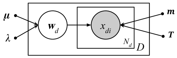
Figure 1: Graphical model for Bayesian SMM

The problem arises while computing the denominator in (4). It involves solving the integral over a product of likelihood term containing the $\mathrm{softmax}$ function and $\mathrm{Gaussian}$ distribution (prior). There exists no analytical form for this integral. This is a generic problem that arises while performing Bayesian inference for mixed-logit models [22, 27], multi-class logistic regression or any other model where likelihood function and prior are not conjugate to each other [16]. In such cases, one can resort to variational inference and find an approximation to the posterior distribution $p(\bm{w}|\bm{x})$. This approximation to the true posterior is referred as variational distribution $q(\bm{w})$, and is obtained by minimizing the Kullback-Leibler (KL) divergence, $D_{\mathrm{KL}}(q\,||\,p)$ between the approximate and true posterior. We can express $\log$ marginal (evidence) of the data as:

$$\log p(\bm{x}) =\mathbb{E}_{q}[\log p(\bm{x},\bm{w})]+\mathrm{H}[q]\,+D_{\mathrm{KL}}(q\,||\,p),$$ (8)

$$=\mathcal{L}(q)+D_{\mathrm{KL}}(q\,||\,p).$$ (9)

Here $\mathrm{H}[q]$ represents the entropy of $q(\bm{w})$. Given the data $\bm{x}$, $\log p(\bm{x})$ is a constant with respect to $\bm{w}$, and $D_{\mathrm{KL}}(q\,||\,p)$ can be minimized by maximizing $\mathcal{L}(q)$, which is known as Evidence Lower BOund (ELBO) for a document. This is the standard formulation of variational Bayes [16], where the problem of finding an approximate posterior is transformed into optimization of the functional $\mathcal{L}(q)$.

III Variational Bayes

In this section, using the VB framework, we derive and explain the procedure for estimating model parameters $\{\bm{m},\bm{T}\}$ and inferring the variational distribution, $q(\bm{w})$. Before proceeding, we note that our model assumes that all documents and the corresponding document embeddings (latent variables) are independent. This can be seen from the graphical model in Fig. 1. Hence, we derive the inference only for one document embedding $\bm{w}$, given an observed vector of word counts $\bm{x}$.

We chose the variational distribution $q(\bm{w})$ to be $\mathrm{Gaussian}$, with mean $\bm{\nu}$ and precision $\bm{\Gamma}$, i.e., $q(\bm{w})=\mathcal{N}(\bm{w}\,|\,\bm{\nu},\,\bm{\Gamma}^{\mkern-1.2mu\mathsf{-1}})$. The functional $\mathcal{L}(q)$ now becomes:

$$\mathcal{L}(q) =\mathbb{E}_{q}[\log p(\bm{x},\bm{w})]\,+\,\mathrm{H}[q],$$ (10)

$$=-\underbrace{D_{\mathrm{KL}}(q\,||\,p)}_{\mathsf{A}}\,+\,\underbrace{\mathbb{E}_{q}[\log p(\bm{x}\mid\bm{w})]}_{\mathsf{B}}.$$ (11)

The term $\mathsf{A}$ from (11) is the negative KL divergence between the variational distribution $q(\bm{w})$ and the document-independent prior from (1). This can be computed analytically [28] as:

$$D_{\mathrm{KL}}(q\,||\,p)=\frac{1}{2}\Big{[}\lambda\tr(\bm{\Gamma}^{{}^{\mkern-1.2mu\mathsf{-1}}})\,+\,\log|\bm{\Gamma}|\,-\,K\log\lambda\\ +\lambda\,\bm{\nu}^{{}^{\mkern-1.2mu\mathsf{T}}}\bm{\nu}-K\Big{]},$$ (12)

where $K$ denotes the document embedding dimensionality. The term $\mathsf{B}$ from (11) is the expectation over $\log$-likelihood of a document (7):

$$\mathbb{E}_{q}[\log p(\bm{x}\,|\,\bm{w})]=\sum_{i=1}^{V}x_{i}\Bigg{[}(m_{i}+\bm{t}_{i}\bm{\nu})\\ -\underbrace{\mathbb{E}_{q}\Big{[}\log(\sum_{j=1}^{V}\exp{m_{j}+\bm{t}_{j}\bm{w}})\Big{]}}_{\mathcal{F}}\Bigg{]}.$$ (13)

(13) involves solving the expectation over $\log$-$\mathrm{sum}$-$\exp$ operation (denoted by $\mathcal{F}$), which is intractable. It appears when dealing with variational inference in mixed-logit models [22, 27]. We can approximate $\mathcal{F}$ with empirical expectation using samples from $q(\bm{w})$, but $\mathcal{F}$ is a function of $q(\bm{w})$, whose parameters we are seeking by optimizing $\mathcal{L}(q)$. The corresponding gradients of $\mathcal{L}(q)$ with respect to $q(\bm{w})$ will exhibit high variance if we directly take samples from $q(\bm{w})$ for the empirical expectation. To overcome this, we will re-parametrize the random variable $\bm{w}$ [14]. This is done by introducing a differentiable function $g$ over another random variable $\bm{\epsilon}$. If $p(\bm{\epsilon})=\mathcal{N}(\bm{0},\bm{I})$, then,

$$\bm{w}=g(\bm{\epsilon})=\bm{\nu}+\bm{L}\,\,\bm{\epsilon},$$ (14)

where $\bm{L}$ is the Cholesky factor of $\bm{\Gamma}^{{}^{\mkern-1.2mu\mathsf{-1}}}$. Using this re-parametrization of $\bm{w}$, we obtain the following approximation:

$$\mathcal{F}\approx\frac{1}{R}\sum_{r=1}^{R}\log(\sum_{j=1}^{V}\exp{m_{j}+\bm{t}_{j}\,g(\tilde{\bm{\epsilon}}_{r})}),$$ (15)

where $R$ denotes the total number of samples $\tilde{\bm{\epsilon}}_{r}$ from $p(\bm{\epsilon})$. Combining (12),(13) and (15), we get the approximation to $\mathcal{L}(q)$. We will introduce the document suffix $d$, to make the notation explicit:

$$\mathcal{L}(q_{d})\approx-D_{\mathrm{KL}}(q_{d}\mid\mid p)+\sum_{i=1}^{V}x_{di}\,\Big{[}\,(m_{i}+\bm{t}_{i}\bm{\nu}_{d})\\ -\frac{1}{R}\sum_{r=1}^{R}\log(\sum_{j=1}^{V}\exp{m_{j}+\bm{t}_{j}\,g(\tilde{\bm{\epsilon}}_{dr})})\Big{]}.$$ (16)

For the entire training data $\bm{X}$, the complete ELBO will be simply the summation over all the documents, i.e., $\sum_{d}\mathcal{L}(q_{d})$.

III-A Training

The variational Bayes (VB) training procedure for Bayesian SMM is stochastic because of the sampling involved in the re-parametrization trick (14). Like the standard VB approach [16], we optimize ELBO alternately with respect to $q(\bm{w})$ and $\{\bm{m},\bm{T}\}$. Since we do not have closed form update equations, we perform gradient-based updates. Additionally, we regularize rows in matrix $\bm{T}$ while optimizing. Thus, the final objective function becomes,

$$\mathcal{L}=\sum_{d=1}^{D}\mathcal{L}(q_{d})-\omega\sum_{i=1}^{V}||\bm{t}_{i}||_{{}_{\mkern 2.0mu\mathsf{1}}}\,,$$ (17)

where we have added the term for $\ell_{1}$ regularization of rows in matrix $\bm{T}$, with corresponding weight $\omega$. The same regularization was previously used for non Bayesian SMM in [20]. This can also be seen as obtaining a maximum a posteriori estimate of $\bm{T}$ with Laplace priors.

III-A1 Parameter initialization

The vector $\bm{m}$ is initialized to $\log$ uni-gram probabilities estimated from training data. The values in matrix $\bm{T}$ are randomly initialized from $\mathcal{N}(0,0.001)$. The prior over latent variables $p(\bm{w})$ is set to isotropic Gaussian distribution with mean $\bm{0}$ and $\lambda=\{1,10\}$. The variational distribution $\bm{q}(w)$ is initialized to $\mathcal{N}(\bm{0},\mathrm{diag}(0.1))$. Later in Section VII-A, we will show that initializing the posterior to a sharper Gaussian distribution helps to speed up the convergence.

III-A2 Optimization

The gradient-based updates are done by adam optimization scheme [23]; in addition to the following tricks:

We simplified the variational distribution $q(\bm{w})$ by making its precision matrix $\bm{\Gamma}$ diagonal. Further, while updating it, we used $\log$ standard deviation parametrization, i.e.,

$$\bm{\Gamma}^{{}^{\mkern-1.2mu\mathsf{-1}}}=\mathrm{diag}(\exp\{2\,\bm{\varsigma}\}).$$ (18)

The gradients of the objective (16) w.r.t. the mean $\bm{\nu}$ is given as follows:

$$\nabla\bm{\nu} =\Big{[}\sum_{i=1}^{V}\bm{t}_{i}^{{}^{\mkern-1.2mu\mathsf{T}}}(x_{i}-\frac{1}{R}\sum_{r=1}^{R}\theta_{ir}\sum_{k=1}^{V}x_{k})\Big{]}-\lambda\bm{\nu}$$ (19)

where,

$$\theta_{ir} =\dfrac{\hfill\exp\{m_{i}+\bm{t}_{j}g(\bm{\epsilon}_{r})\}}{\sum_{j}\exp\{m_{j}+\bm{t}_{j}g(\bm{\epsilon}_{r})\}}$$ (20)

The gradient w.r.t $\log$ standard deviation $\bm{\varsigma}$ is given as:

$$\nabla\bm{\varsigma}=\bm{1}-\lambda\exp\{2\bm{\varsigma}\}\,\\ -\sum_{k=1}^{V}x_{k}\frac{1}{R}\sum_{r=1}^{R}\sum_{i=1}^{V}\theta_{ir}\bm{t}_{i}^{{}^{\mkern-1.2mu\mathsf{T}}}\odot\exp\{\bm{\varsigma}\}\odot\bm{\epsilon}_{r},$$ (21)

where $\bm{1}$ represents a column vector of ones, $\odot$ denotes element-wise product, and $\exp$ is element-wise exponential operation.

The $\ell_{1}$ regularization term makes the objective function (17) discontinuous (non-differentiable) at points where it crosses the orthant. Hence, we used sub-gradients and employed orthant-wise learning [24]. The gradient of the objective (17) w.r.t. a row $\bm{t}_{i}$ in matrix $\bm{T}$ is computed as follows:

$$\nabla\bm{t}_{i}=-\omega\,\mathrm{sign}(\bm{t}_{i})+\sum_{d=1}^{D}\Bigg{[}x_{di}\bm{\nu}_{d}^{{}^{\mkern-1.2mu\mathsf{T}}}-\\ \Big{[}\Big{(}\sum_{k=1}^{V}x_{ki}\Big{)}\frac{1}{R}\sum_{r=1}^{R}\theta_{dir}(\bm{\nu}_{d}^{{}^{\mkern-1.2mu\mathsf{T}}}+\bm{\epsilon}_{dr}^{{}^{\mkern-1.2mu\mathsf{T}}}\odot\exp\{\bm{\varsigma}^{{}^{\mkern-1.2mu\mathsf{T}}}\})\Big{]}\Bigg{]}.$$ (22)

Here, $\mathrm{sign}$ and $\exp$ operate element-wise. The sub-gradient $\tilde{\nabla}\bm{t}_{i}$ is defined as:

$$\tilde{\nabla}{t}_{ik}\triangleq\left\{\begin{array}[]{lcccl}\nabla{t}_{ik}+\omega,&\quad t_{ik}&=0,&\nabla{t}_{ik}&<-\omega\\ \nabla{t}_{ik}-\omega,&\quad t_{ik}&=0,&\nabla{t}_{ik}&>\omega\\ 0,&\quad t_{ik}&=0,&|\nabla{t}_{ik}|&\leq\omega\\ \nabla{t}_{ik},&\quad|t_{ik}|&>0&.\end{array}\right.$$ (23)

Finally, the rows in matrix $\bm{T}$ are updated according to,

$$\bm{t}_{i} \leftarrow\mathcal{P_{O}}(\bm{t}_{i}+\bm{d}_{i})\,$$ (24)

where, $$\bm{d}_{i}$$ is the step in ascent direction,

$$\bm{d}_{i} =\eta\,\mathrm{diag}(\sqrt{\bm{s}_{i}}+\epsilon)^{{}^{\mkern-1.2mu\mathsf{-1}}}\,\bm{f}_{i}\,.$$ (25)

Here, $\eta$ is the learning rate, $\bm{f}_{i}$ and $\bm{s}_{i}$ represents bias corrected first and second moments (as required by adam) of sub-gradient $\tilde{\nabla}\bm{t}_{i}$ respectively. $\mathcal{P}_{O}$ represents orthant projection, which ensures that the update step does not cross the point of non-differentiability. It is defined as,

$$\mathcal{P_{O}}(\bm{t}_{i}+\bm{d}_{i})\triangleq\left\{\begin{array}[]{ll}0&\textrm{if}\quad t_{ik}(t_{ik}+d_{ik})<0,\\ t_{ik}+d_{ik}&\textrm{otherwise}\,.\end{array}\right.$$ (26)

The orthant projection introduces explicit zeros in the estimated $\bm{T}$ matrix and, results in sparse solution. Unlike in [20], we do not require to apply the sign projection, because both the gradient $\tilde{\nabla}\bm{t}_{i}$ and step $\bm{d}$ point to the same orthant (due to properties of adam). The stochastic VB training is outlined in Algorithm 1.

1 initialize the model and the variational parameters

2 repeat

3       for $d=1\ldots D\,$ do

4             sample $\tilde{\bm{\epsilon}}_{dr}\sim\mathcal{N}(\bm{0},\bm{I})\qquad r=1\ldots R$

5             compute $\mathcal{L}(q_{d})$ using (16)

6             compute gradient $\nabla\bm{\nu}_{d}$ using (19)

7             compute gradient $\nabla\bm{\varsigma}_{d}$ using (21)

8             update $\bm{\nu}_{d}$ and $\bm{\varsigma}_{d}$ using adam

9            

10       end for

11      compute $\mathcal{L}$ using (17)

12       compute sub-gradients $\tilde{\nabla}\bm{t}_{i}$ using (22) and (23)

13       update rows in $\bm{T}$ using (24)

14      

15until convergence or max_iterations

Algorithm 1 Stochastic VB training

III-B Inferring embeddings for new documents

After obtaining the model parameters from VB training, we can infer (extract) the posterior distribution of document embedding $q(\bm{w})$ for any given document $\bm{x}$. This is done by iteratively updating the parameters of $q(\bm{w})$ that maximize $\mathcal{L}(q)$ from (16). These updates are performed by following the same adam optimization scheme as in training.

Note that the embeddings are extracted by maximizing the ELBO, that does not involve any supervision (topic labels). These embeddings which are in the form of posterior distributions will be used as input features for training topic ID classifiers. Alternatively, one can use only the mean of the posterior distributions as point estimates of document embeddings.

IV Gaussian classifier with uncertainty

In this section, we will present a generative Gaussian classifier that exploits the uncertainty in posterior distributions of document embedding. Moreover, it also exploits the same uncertainty while computing the posterior probability of class labels. The proposed classifier is called Gaussian linear classifier with uncertainty (GLCU) and is inspired by [29, 30]. It can be seen as an extension to the simple Gaussian linear classifier (GLC) [16].

Let $\ell=1\ldots L$ denote class labels, $d=1\ldots D$ represent document indices, and $\bm{h}_{d}$ represent the class label of document $d$ in one-hot encoding.

GLC assumes that every class is Gaussian distributed with a specific mean $\bm{\mu}_{\ell}$, and a shared precision matrix $\bm{D}$. Let $\bm{M}$ denote a matrix of class means, with $\bm{\mu}_{\ell}$ representing a column. GLC is described by the following model:

$$\bm{w}_{d}=\bm{\mu}_{d}+\bm{\varepsilon}_{d},\\$$ (27)

where $\bm{\mu}_{d}=\bm{M}\bm{h}_{d}$, $p(\bm{\varepsilon})=\mathcal{N}(\bm{\varepsilon}\,|\,\bm{0},\bm{D}^{{}^{\mkern-1.2mu\mathsf{-1}}})$ and $\bm{w}_{d}$ represent embedding for document $d$. GLC can be trained by estimating the parameters $\varTheta=\{\bm{M},\bm{D}\}$ that maximize the class conditional likelihood of all training examples:

$$\prod_{d=1}^{D}p(\bm{w}_{d}\,|\,\bm{h}_{d},\varTheta)=\prod_{d=1}^{D}\mathcal{N}(\bm{w}_{d}\,|\,\bm{\mu}_{d},\bm{D}^{{}^{\mkern-1.2mu\mathsf{-1}}}).$$ (28)

In our case, however, the training examples come in the form of posterior distributions, $q(\bm{w}_{d})=\mathcal{N}(\bm{w}_{d}\,|\,\bm{\nu}_{d},\bm{\Gamma}_{d}^{{}^{\mkern-1.2mu\mathsf{-1}}})$ as extracted using our Bayesian SMM. In such case, the proper ML training procedure should maximize the expected class-conditional likelihood, with the expectation over $\bm{w}_{d}$ calculated for each training example with respect to its posterior distribution $q(\bm{w}_{d})$ i.e., $\mathbb{E}_{q}[\mathcal{N}(\bm{w}_{d}\,|\,\bm{\mu}_{d},\bm{D}^{{}^{\mkern-1.2mu\mathsf{-1}}})]$.

However, it is more convenient to introduce an equivalent model, where the observations are the means $\bm{\nu}_{d}$ of the posteriors $q(\bm{w}_{d})$ and the uncertainty encoded in $\bm{\Gamma}_{d}^{{}^{\mkern-1.2mu\mathsf{-1}}}$ is introduced into the model through the latent variable $\bm{y}_{d}$ as,

$$\bm{\nu}_{d}=\bm{\mu}_{d}+\bm{y}_{d}+\bm{\varepsilon}_{d},$$ (29)

where, $p(\bm{y}_{d})=\mathcal{N}(\bm{y}_{d}\,|\,\bm{0},\bm{\Gamma}_{d}^{{}^{\mkern-1.2mu\mathsf{-1}}})$. The resulting model is called GLCU. Since the random variables $\bm{y}_{d}$ and $\bm{\epsilon}_{d}$ are Gaussian-distributed, the resulting class conditional likelihood is obtained using convolution of two Gaussians [16], i.e,

$$p(\bm{\nu}_{d}\,|\,\bm{h}_{d},\varTheta)=\mathcal{N}(\bm{\nu}_{d}\,|\,\bm{\mu}_{d},\,\bm{\Gamma}_{d}^{{}^{\mkern-1.2mu\mathsf{-1}}}+\bm{D}^{{}^{\mkern-1.2mu\mathsf{-1}}}).$$ (30)

GLCU can be trained by estimating its parameters $\varTheta$, that maximize the class conditional likelihood of training data (30). This can be done efficiently by using the following em algorithm.

IV-A EM algorithm

In the e-step, we calculate the posterior distribution of latent variables:

$$p(\bm{y}_{d}\,|\,\bm{\nu}_{d},\bm{h}_{d},\varTheta) \propto p(\bm{\nu}_{d}\,|\,\bm{y}_{d},\bm{h}_{d}\varTheta)\,\,p(\bm{y}_{d})$$

$$\propto\,\mathcal{N}(\bm{y}_{d}\,|\,\bm{u}_{d},\bm{V}^{{}^{\mkern-1.2mu\mathsf{-1}}}_{d}),$$ (31)

where,

$$\bm{V}_{d} =\bm{D}+\bm{\Gamma}_{d},$$ (32)

$$\bm{u}_{d} =[\bm{I}+\bm{D}^{{}^{\mkern-1.2mu\mathsf{-1}}}\bm{\Gamma}_{d}]^{{}^{\mkern-1.2mu\mathsf{-1}}}(\bm{\nu}_{d}-\bm{\mu}_{d}).$$ (33)

In the m-step, we maximize the auxiliary function $\mathcal{Q}$ with respect to model parameters $\varTheta$. It is the expectation of $\log$ joint-probability with respect to $p(\bm{y}_{d}\,|\,\bm{\nu}_{d})$, i.e.,

$$\mathcal{Q} =\mathbb{E}_{p}[\sum_{d=1}^{D}\log p(\bm{\nu}_{d},\bm{y}_{d}\mid\varTheta)]$$ (34)

$$=\frac{-D}{2}\log|\bm{D}|-\frac{1}{2}\Bigg{[}\sum_{d=1}^{D}\Big{(}\mathrm{tr}(\bm{D}\bm{V}_{d}^{{}^{\mkern-1.2mu\mathsf{-1}}})$$

$$\,+\big{(}\bm{u}_{d}-(\bm{\nu}_{d}-\bm{\mu}_{d})\big{)}^{{}^{\mkern-1.2mu\mathsf{T}}}\bm{D}\big{(}\bm{u}_{d}-(\bm{\nu}_{d}-\bm{\mu}_{d})\big{)}\Big{)}\Bigg{]}+\mathrm{const}.$$ (35)

Maximizing the auxiliary function $\mathcal{Q}$ w.r.t. $\varTheta$, we have:

$$\bm{\mu}_{\ell} :=\frac{1}{|\mathcal{I}_{\ell}|}\sum_{d\in\mathcal{I}_{\ell}}(\bm{\nu}_{d}-\bm{u}_{d})\quad\forall\,\ell=1\ldots L$$ (36)

$$\bm{D}^{{}^{\mkern-1.2mu\mathsf{-1}}} :=\frac{1}{D}\Big{[}\sum_{d=1}^{D}(\bm{a}_{d}\,\bm{a}^{{}^{\mkern-1.2mu\mathsf{T}}}_{d})+\bm{V}_{d}^{{}^{\mkern-1.2mu\mathsf{-1}}}\Big{]},$$ (37)

where, $\bm{a}_{d}=\bm{u}_{d}-(\bm{\nu}_{d}-\bm{\mu}_{d})$, and, $\mathcal{I}_{\ell}$ is the set of documents from class $\ell$. To train the GLCU model, we alternate between e-step and m-step until convergence.

IV-B Classification

Given a test document embedding posterior distribution $q(\bm{w})=\mathcal{N}(\bm{w}\,|\,\bm{\nu},\bm{\Gamma}^{{}^{\mkern-1.2mu\mathsf{-1}}})$, we compute the class conditional likelihood according to (30), and the posterior probability of a class $\mathcal{C}_{k}$ is obtained by applying the Bayes’ rule:

$$p(\mathcal{C}_{k}\,|\,\bm{\nu},\bm{\Gamma},\varTheta)=\dfrac{\hfill p(\bm{\nu}\mid\bm{\mu}_{k},\bm{D},\bm{\Gamma})\,p(\mathcal{C}_{k})}{\sum_{\ell}p(\bm{\nu}\mid\bm{\mu}_{\ell},\bm{D},\bm{\Gamma})\,p(\mathcal{C}_{\ell})}.$$ (38)

V Related models

In this section, we review and relate some of the popular PTMs and neural network based document models. We begin with a brief review of LDA [21], a probabilistic generative model for bag-of-words representation of documents.

V-A Latent Dirichlet allocation

Let $\bm{\phi}_{1:K}$ represent $K$ topics. LDA assumes that every topic $\bm{\phi}_{k}$ is a distribution over a fixed vocabulary of size $V$. Every document $d$ is generated by a two step process: First, a document-specific vector (embedding) representing a distribution over $K$ topics is sampled, i.e., $\bm{\theta}_{d}\sim\mathrm{Dir}(\bm{\alpha})$. Then, for each word in the document $d$, a topic indicator variable $z_{i}$ is sampled: $z_{i}\sim\mathrm{Multi}(\bm{\theta}_{d};1)$ and the word $x_{i}$ is in turn sampled from the topic-specific distribution: $x_{i}\sim\mathrm{Multi}(\bm{\phi}_{z_{i}};1)$.

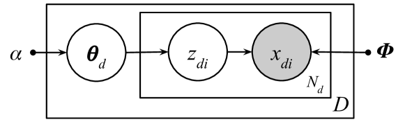
Figure 2: Graphical model for LDA

The topic ($\bm{\phi}$) and document ($\bm{\theta}$) vectors live in $(V-1)$ and $(K-1)$ simplexes respectively. For every word $x_{i}$ in document $d$, there is a discrete latent variable $z_{i}$ that tells which topic was responsible for generating the word. This can be seen from the respective graphical model in Fig. 2.

During inference, the generative process is inverted to obtain posterior distribution over latent variables, $p(\bm{\theta},\bm{z}\,|\,\bm{x},\bm{\alpha},\bm{\phi}_{1:K})$, given the observed data and prior belief. Since the true posterior is intractable, Blei [21] resorted to variational inference which finds an approximation to the true posterior as a variational distribution $q(\bm{\theta},\bm{z})$. Further, mean-field approximation was made to make the inference tractable, i.e., $q(\bm{\theta},\bm{z})=q(\bm{\theta})\prod_{i}q(z_{i})$.

In the original model proposed by Blei [21], the parameters $\bm{\phi}$ were obtained using maximum likelihood approach. The choice of $\mathrm{Dirichlet}$ distribution for $q(\bm{\theta})$ simplifies the inference process because of the $\mathrm{Dirichlet}$-$\mathrm{Multinomial}$ conjugacy. However, the assumption of $\mathrm{Dirichlet}$ distribution causes limitations to the model, and $q(\bm{\theta})$ cannot capture correlations between topics in each document. This was the motivation for Blei [22] to model documents with $\mathrm{Gaussian}$ distributions, and the resulting model is called correlated topic model (CTM).

V-B Correlated topic model

The generative process for a document in CTM [22] is same as in LDA, except for document vectors are now drawn from $\mathrm{Gaussian}$, i.e.,

$$p(\bm{\eta}) =\mathcal{N}(\bm{\eta}\mid\bm{\mu},\mathrm{diag}(\lambda)^{{}^{\mkern-1.2mu\mathsf{-1}}}),$$ (39)

$$\bm{\theta} =\mathrm{softmax}(\bm{\eta}).$$ (40)

In this formulation, the document embeddings $\bm{\eta}$ are no longer in the $(K-1)$ simplex, rather they are dependent through the logistic normal. This is the same as in our proposed Bayesian SMM (1). The advantage is that the document vectors can model the correlations in topics. The topic distributions over vocabulary $\bm{\phi}$, however, still remained $\mathrm{Discrete}$. In Bayesian SMM, the topic-word distributions ($\bm{T}$) are not $\mathrm{Discrete}$ , hence it can model the correlations between words and (latent) topics [22].

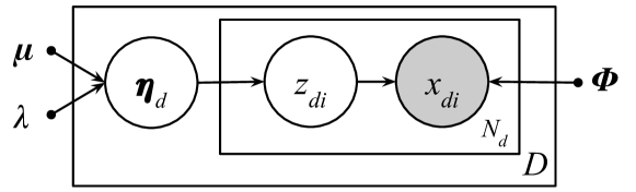
Figure 3: Graphical model for CTM

The variational inference in CTM is similar to that of LDA including the mean-field approximation, because of the discrete latent variable $\bm{z}$ (Fig. 3). An additional problem is dealing with the non-conjugacy. More specifically, it is the intractability while solving the expectation over $\log$-$\mathrm{sum}$-$\exp$ function (see $\mathcal{F}$ from (13)). Blei [22] used Jensen’s inequality to form an upper bound on $\mathcal{F}$, and this in-turn acted as lower bound on ELBO. In our proposed Bayesian SMM, we also encountered the same problem, and we approximated $\mathcal{F}$ using the re-parametrization trick (Section III). There exist similar approximation techniques based on Quasi Monte Carlo sampling [27].

Unlike in LDA or CTM, Bayesian SMM does not require to make mean-field approximation, because the topic-word mixture is not $\mathrm{Discrete}$ thus eliminating the need for discrete latent variable $\bm{z}$.

V-C Subspace multinomial model

SMM is a log-linear model; originally proposed for modelling discrete prosodic features for the task of speaker verification [25]. Later, it was used for phonotatic language recognition [31] and eventually for topic identification and document clustering [19, 20]. Similar model was proposed by Maas [32] for unsupervised learning of word representations. One of the major differences among these works is the type of regularization used for matrix $\bm{T}$.

Another major difference is in obtaining embeddings $\bm{w}_{d}$ for a given test document. Maas [32] obtained them by projecting the vector of word counts $\bm{x}_{d}$ onto the matrix $\bm{T}$, i.e., $\bm{w}_{d}=\bm{T\,x}_{d}$, whereas [19, 20] extracted the embeddings by maximizing regularized $\log$-likelihood function. The embeddings extracted using SMM are prone to over-fitting. Our Bayesian SMM overcomes this problem by capturing the uncertainty of document embeddings in the posterior distribution. Our experimental analysis in section VII-C illustrates the robustness of Bayesian SMM.

V-D Paragraph vector

Paragraph vector bag-of-words (PV-DBOW) [8] is also a log-linear model, which is trained stochastically to maximize the likelihood of a set of words from a given document. SMM can be seen as a special case of PV-DBOW, since it maximizes the likelihood of all the words in a document.

V-E Neural network based models

Neural variational document model (NVDM) is an adaptation of variational auto-encoders for document modelling [15]. The encoder models the posterior distribution of latent variables given the input, i.e., $p_{\theta}(\bm{z}\,|\,\bm{x})$, and the decoder models distribution of input data given the latent variable, i.e., $p_{\theta}(\bm{x}\,|\,\bm{z})$. In NVDM, the authors used bag-of-words as input, while their encoder and decoders are two-layer feed-forward neural networks. The decoder part of NVDM is similar to Bayesian SMM, as both the models maximize expected $\log$-likelihood of data, assuming $\mathrm{Multinomial}$ distribution. In simple terms, Bayesian SMM is a decoder with a single feed forward layer. For a given test document, in NVDM, the approximate posterior distribution of latent variables is obtained directly by forward propagating through the encoder; whereas in Bayesian SMM, it is obtained by iteratively optimizing ELBO. The experiments in Section VII show that the posterior distributions obtained from Bayesian SMM represent the data better as compared to the ones obtained directly from the encoder of NVDM.

V-F Sparsity in topic models

Sparsity is often one of the desired properties in topic models [33, 34]. Sparse coding inspired topic model was proposed by [35], where the authors have obtained sparse representations for both documents and words. $\ell_{1}$ regularization over $\bm{T}$ for SMM ($\ell_{1}$ SMM) was observed to yield better results when compared to LDA, STC and $\ell_{2}$ regularized SMM ($\ell_{2}$ SMM) [20]. Relation between SMM and sparse additive generative model (SAGE) [33] was explained in [19]. In [36], the authors proposed an algorithm to obtain sparse document embeddings (called sparse composite document vector (SCDV)) from pre-trained word embeddings. In our proposed Bayesian SMM, we introduce sparsity into the model parameters $\bm{T}$ by applying $\ell_{1}$ regularization and using orthant-wise learning.

VI Experiments

VI-A Datasets

We have conducted experiments on both speech and text corpora. The speech data used is Fisher phase 1 corpus, which is a collection of 5850 conversational telephone speech recordings with a closed set of 40 topics. Each conversation is approximately 10 minutes long with two sides of the call and is supposedly about one topic. We considered each side of the call (recording) as an independent document, which resulted in a total of 11700 documents. Table I presents the details of data splits; they are the same as used in earlier research [37, 38, 19]. Our preprocessing involved removing punctuation and special characters, but we did not remove any stop words. Using Kaldi open-source toolkit [39], we trained a sequence discriminative DNN-HMM automatic speech recognizer (ASR) system [40] to obtain automatic transcriptions. The ASR system resulted in 18% word-error-rate on a held-out test set. We report experimental results on both manual and automatic transcriptions. The vocabulary size while using manual transcriptions was 24854, for automatic, it was 18292, and the average document length is 830, and 856 words respectively.

TABLE I: Data splits from Fisher phase 1 corpus, where each document represents one side of the conversation.

Set	# docs.	Duration (hrs.)
ASR training	6208	553
Topic ID training	2748	244
Topic ID test	2744	226

The text corpus used is 20Newsgroups, which contains 11314 training and 7532 test documents over 20 topics. Our preprocessing involved removing punctuation and words that do not occur in at least two documents, which resulted in a vocabulary of 56433 words. The average document length is 290 words.

VI-B Hyper-parameters of Bayesian SMM

In our topic ID experiments, we observed that the embedding dimension ($K$) and regularization weight ($\omega$) for rows in matrix $\bm{T}$ are the two important hyper-parameters. The embedding dimension was chosen from $K=\{100,\ldots,800\}$, and regularization weight from $\omega=\{0.0001,\ldots,10.0\}$.

VI-C Proposed topic ID systems

Our Bayesian SMM is an unsupervised model trained iteratively by optimizing the ELBO; it does not necessarily correlate with the performance of topic ID. It is valid for SMM, NVDM or any other generative model trained without supervision. A typical way to overcome this problem is to have an early stopping mechanism (ESM), which requires to evaluate the topic ID accuracy on a held-out (or cross-validation) set at regular intervals during the training. It can then be used to stop the training earlier if needed.

Using the above described scheme, we trained three different classifiers: (i) Gaussian linear classifier (GLC), (ii) multi-class logistic regression (LR), and, (iii) Gaussian linear classifier with uncertainty (GLCU). Note that GLC and LR cannot exploit the uncertainty in the document embeddings; and are trained using only the mean parameter $\bm{\nu}$ of the posterior distributions; whereas GLCU is trained using the full posterior distribution $q(\bm{w})$, i.e., along with the uncertainties of document embeddings as described in Section IV. GLC and GLCU does not have any hyper-parameters to tune, while the $\ell_{2}$ regularization weight of LR was tuned using cross-validation experiments.

VI-D Baseline topic ID systems

VI-D1 NVDM

Since NVDM and our proposed Bayesian SMM share similarities, we chose to extract the embeddings from NVDM and use them for training linear classifiers. Given a trained NVDM model, embeddings for any test document can be extracted just by forward propagating through the encoder. Although this is computationally cheaper, one needs to decide when to stop training, as a fully converged NVDM may not yield optimal embeddings for discriminative tasks such as topic ID. Hence, we used the same early stopping mechanism as described in earlier section. We used the same three classifier pipelines (LR, GLC, GLCU) as we used for Bayesian SMM. Our architecture and training scheme are similar to ones proposed in [15], i.e., two feed forward layers with either $500$ or $1000$ hidden units and $\{\mathrm{sigmoid},\mathrm{ReLU},\mathrm{tanh}\}$ activation functions. The latent dimension was chosen from $K=\{100,\ldots,800\}$. The hyper-parameters were tuned based on cross-validation experiments.

VI-D2 SMM

Our second baseline system is non-Bayesian SMM with $\ell_{1}$ regularization over the rows in $\bm{T}$ matrix, i.e., $\ell_{1}$ SMM. It was trained with hyper-parameters such as embedding dimension $K=\{100,\ldots,800\}$, and regularization weight $\omega=\{0.0001,\ldots,10.0\}$. The embeddings obtained from SMM were then used to train GLC and LR classifiers. Note that we cannot use GLCU here, because SMM yields only point-estimates of embeddings. We used the same early stopping mechanism to train the classifiers. The experimental analysis in Section VII-C shows that Bayesian SMM is more robust to over-fitting when compared to SMM and NVDM, and does not require an early stopping mechanism.

VI-D3 ULMFiT

The third baseline system is the universal language model fine-tuned for classification (ULMFiT) [9]. The pre-trained model consists of 3 BiLSTM layers. Fine-tuning the model involves two steps: (a) fine-tuning LM on the target dataset and (b) training classifier (MLP layer) on the target dataset. We trained several models with various drop-out rates. More specifically, the LM was fine-tuned for 15 epochs, with drop-out rates from: $\{0.2,\ldots,0.6\}$. The classifier was fine-tuned for 50 epochs with drop-out rates from: $\{0.2,\ldots,0.6\}$. A held-out development set was used to tune the hyper-parameters (drop-out rates, and fine-tuning epochs).

VI-D4 TF-IDF

The fourth baseline system is a standard term frequency-inverse document frequency (TF-IDF) based document representation, followed by multi-class logistic regression (LR). Although TF-IDF is not a topic model, the classification performance of TF-IDF based systems are often close to state-of-the-art systems [19]. The hyper-parameter ($\ell_{2}$ regularization weight) of LR was selected based on 5-fold cross-validation experiments on training set.

VII Results and Discussion

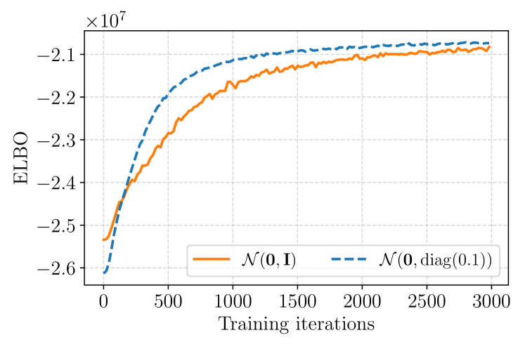
Figure 4: Convergence of Bayesian SMM for various initializations of variational distribution. The model was trained on 20Newsgroups corpus with $K=100$, and $\omega=1$.

VII-A Convergence rate of Bayesian SMM

We observed that the posterior distributions extracted using Bayesian SMM are always much sharper than standard Normal distribution. Hence we initialized the variational distribution to $\mathcal{N}(\bm{0},\,\mathrm{diag}(0.1))$ to speed up the convergence. Fig. 4 shows objective (ELBO) plotted for two different initializations of variational distribution. Here, the model was trained on 20Newsgroups corpus, with the embedding dimension $K=100$, regularization weight $\omega=1.0$ and prior set to standard $\mathrm{Normal}$. We can observe that the model initialized to $\mathcal{N}(\bm{0},\,\mathrm{diag}(0.1))$ converges faster as compared to the one initialized to standard $\mathrm{Normal}$. In all the further experiments, we initialized both the prior and variational distributions to $\mathcal{N}(\bm{0},\,\mathrm{diag}(0.1))$.

VII-B Perplexity

Perplexity is an intrinsic measure for topic models [41, 15]. It is computed as an average of every test document according to:

PPL_DOC $$=\exp\{\dfrac{-1}{\hfill D}\sum_{d=1}^{D}\frac{\log p(\bm{x}_{d})}{N_{d}}\Big{\}},$$ (41)

or for an entire test corpus according to:

PPL_CORPUS $$=\exp\{-\frac{\sum_{d=1}^{D}\log p(\bm{x}_{d})}{\sum_{d=1}^{D}N_{d}}\Big{\}},$$ (42)

where $N_{d}$ is the number of word tokens in document $d$.

TABLE II: Comparison of perplexity (PPL) results on 20Newsgroups. The values in the brackets indicate results with a limited vocabulary of 2000 words.

Model	$K$	PPLCORPUS	PPLDOC
NVDM	50	1287 (769)	1421 (820)
NVDM	200	1387 (852)	1519 (870)
Bayesian SMM	50	1043 (629)	1064 (639)
Bayesian SMM	200	882 (519)	851 (515)
ML estimate	-	153 (90)	93 (42)

In our case, $\log p(\bm{x})$ from (9) cannot be evaluated, because the KL divergence from variational distribution $q$ to the true posterior $p$ cannot be computed; as the true posterior is intractable (4). We can only compute $\mathcal{L}(q)$, which is a lower bound on $\log p(x)$; thus the resulting perplexity values act as upper bounds. This is true for NVDM [15] or any other model in the VB framework where the true posterior is intractable [16]. We estimated $\mathcal{L}(q)$ from (16) using $32$ samples, i.e., $R=32$, in order to compute perplexity. In [15], the authors used $20$ samples.

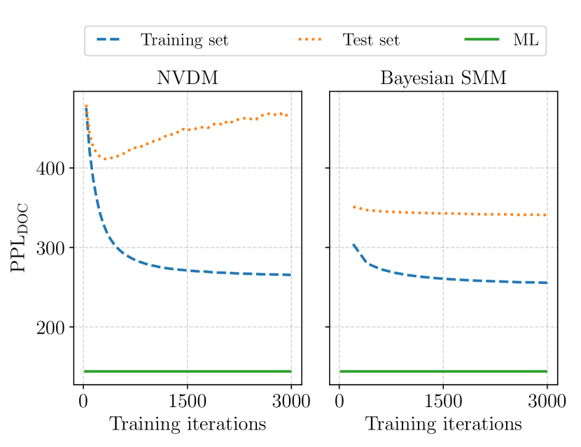
(a) PPL of Fisher test data.

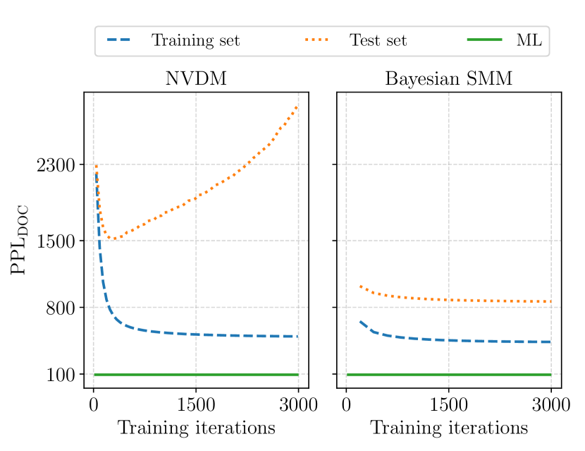
(b) PPL of 20Newsgroups test data.

Figure 5: Comparison of training and test data perplexities obtained using Bayesian SMM and NVDM for both Fisher and 20Newsgroups datasets. The horizontal solid green line shows the test data perplexity computed using the maximum likelihood (ML) probabilities estimated on the test data. The latent (embedding) dimension was set to $200$ for both the models.

We present the comparison of 20Newsgroups test data perplexities obtained using Bayesian SMM and NVDM in Table II. It shows the perplexities of 20Newsgroups corpus under full and a limited vocabulary of 2000 words [15]. We also show the perplexity computed using the maximum likelihood probabilities estimated on the test data. It acts as the lower bound on the test perplexities. NVDM was shown [15] to achieve superior perplexity scores when compared to LDA, docNADE [42], Deep Auto Regressive Neural Network models [43]. To the best of our knowledge, our model achieves state-of-the-art perplexity scores on 20Newsgroups corpus under limited and full vocabulary conditions.

In further investigation, we trained both Bayesian SMM and NVDM until convergence. At regular checkpoints during the training, we froze the model, extracted the embeddings for both training and test data, and computed the perplexities; shown in Figures 5(a) and 5(b). We can observe that both the Bayesian SMM and NVDM fit the training data equally well (low perplexities). However, in the case of NVDM, the perplexity of test data increases after certain number of iterations; suggesting that NVDM fails to generalize and over-fits on the training data. In the case of Bayesian SMM, the perplexity of the test data decreases and remains stable, illustrating the robustness of our model.

VII-C Early stopping mechanism for topic ID systems

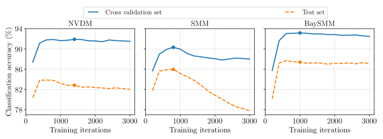
Figure 6: Performance of topic ID systems on Fisher data at various checkpoints during model training. The circular dot ($\bullet$) represents the best cross-validation score and the corresponding test score obtained using the early stopping mechanism (ESM). The embedding dimension was set to 100 for all the models.

The embeddings extracted from a model trained purely in an unsupervised fashion does not necessarily yield optimum results when used in a supervised scenario. As discussed earlier in Sections VI-C, and VI-D, an early stopping mechanism (ESM) during the training of an unsupervised model (eg: NVDM, SMM, and Bayesian SMM) is required to get optimal performance from the subsequent topic ID system. The following experiment illustrates the idea of ESM:

We trained SMM, Bayesian SMM and NVDM on Fisher data until convergence. At regular checkpoints during the training, we froze the model, extracted the embeddings for both training and test data. We chose GLC for SMM, GLCU for NVDM, and Bayesian SMM as topic ID classifiers. We then evaluated the topic ID accuracy on the cross-validation and test sets. Fig. 6 shows the topic ID accuracy on cross-validation and test sets obtained at regular checkpoints for all the three models. The circular dot ($\bullet$) represents the best cross-validation score and the corresponding test score that is obtained by employing ESM. In case of (non-Bayesian) SMM, the test accuracy drops significantly after certain number of iterations; suggesting the strong need of ESM. The cross-validation accuracies of NVDM and Bayesian SMM are similar and remain consistent over the iterations. However, the test accuracy of NVDM is much lower than that of Bayesian SMM and also decreases over the iterations. On the other hand, the test accuracy of Bayesian SMM increases and stays consistent. It shows the robustness of our proposed model, which in addition, does not require any ESM. In all the further topic ID experiments, we report classification results for Bayesian SMM without ESM; while the results for SMM, and NVDM are with ESM.

VII-D Topic ID results

TABLE III: Comparison of results on Fisher test sets, from earlier published works, our baselines and proposed systems. $\star$ indicates a pure discriminative model.

Systems	Model	Classifier	Accuracy (%)	CE	Accuracy (%)	CE
			Manual transcriptions		Automatic transcriptions
Prior works	BoW [37]	NB	87.61	-	-	-
	TF-IDF  [19]	LR	86.41	-	-	-
Our Baseline	TF-IDF	LR	86.59	0.93	86.77	0.94
	ULMFiT $\star$	MLP	86.41	0.50	86.08	0.50
	$\ell_{1}$ SMM	LR	86.81	0.91	87.02	1.09
	$\ell_{1}$ SMM	GLC	85.17	1.64	85.53	1.54
	NVDM	LR	81.16	0.94	83.67	1.15
	NVDM	GLC	84.47	1.25	84.15	1.22
	NVDM	GLCU	83.96	0.93	83.01	0.97
Proposed	Bayesian SMM	LR	89.91	0.89	88.23	0.95
	Bayesian SMM	GLC	89.47	1.05	87.23	1.46
	Bayesian SMM	GLCU	89.54	0.68	87.54	0.77

This section presents the topic ID results in terms of classification accuracy (in %) and cross-entropy (CE) on the test sets. Cross-entropy gives a notion of how confident the classifier is about its prediction. A well calibrated classifier tends to have lower cross-entropy.

Table III presents the classification results on Fisher speech corpora with manual and automatic transcriptions, where the first two rows are the results from earlier published works. Hazen [37], used discriminative vocabulary selection followed by a naïve Bayes (NB) classifier. Having a limited (small) vocabulary is the major drawback of this approach. Although we have used the same training and test splits, May [19] had slightly larger vocabulary than ours, and their best system is similar to our baseline TF-IDF based system. The remaining rows in Table III show our baselines and proposed systems. We can see that our proposed systems achieve consistently better accuracies; notably, GLCU which exploits the uncertainty in document embeddings has much lower cross-entropy than its counter part, GLC. To the best of our knowledge, the proposed systems achieve the best classification results on Fisher corpora with the current set-up, i.e., treating each side of the conversation as an independent document. It can be observed ULMFiT has the lowest cross-entropy among all the systems.

Table IV presents classification results on 20Newsgroups dataset. The first three rows give the results as reported in earlier works. Pappagari et al. [44], proposed a CNN-based discriminative model trained to jointly optimize categorical cross-entropy loss for classification task along with binary cross-entropy for verification task. Sparse composite document vector (SCDV) [36] exploits pre-trained word embeddings to obtain sparse document embeddings, whereas neural tensor skip-gram model (NTSG) [45] extends the idea of a skip-gram model for obtaining document embeddings. The authors in (SCDV) [36] have shown superior classification results as compared to paragraph vector, LDA, NTSG, and other systems. The next rows in Table IV present our baselines and proposed systems. We see that the topic ID systems based on Bayesian SMM and logistic regression is better than all the other models, except for the purely discriminative CNN model. We can also see that all the topic ID systems based on Bayesian SMM are consistently better than variational auto encoder inspired NVDM, and (non-Bayesian) SMM.

The advantages of the proposed Bayesian SMM are summarized as follows: (a) the document embeddings are Gaussian distributed which enables to train simple generative classifiers like GLC, or GLCU; that can extended to newer classes easily, (b) although the Bayesian is trained in an unsupervised fashion, it does not require any early stopping mechanism to yield optimal topic ID results; document embeddings extracted from a fully converged or model can be directly used for classification tasks without any fine-tuning.

TABLE IV: Comparison of results on 20Newsgroups from earlier published works, our baselines and proposed systems. $\star$ indicates a pure discriminative model.

Systems	Model	Classifier	Accuracy (%)	CE
Prior works	CNN [44] $\star$	-	86.12	-
	SCDV [36]	SVM	84.60	-
	NTSG-1 [45]	SVM	82.60	-
Our Baselines	TF-IDF	LR	84.47	0.73
	ULMFiT $\star$	MLP	83.06	0.89
	$\ell_{1}$ SMM	LR	82.01	0.75
	$\ell_{1}$ SMM	GLC	82.02	1.33
	NVDM	LR	79.57	0.86
	NVDM	GLC	77.60	1.65
	NVDM	GLCU	76.86	0.88
Proposed	Bayesian SMM	LR	84.65	0.53
	Bayesian SMM	GLC	83.22	1.28
	Bayesian SMM	GLCU	82.81	0.79

VII-E Uncertainty in document embeddings

The uncertainty captured in the posterior distribution of document embeddings correlates strongly with size of the document. The trace of the covariance matrix of the inferred posterior distributions gives us the notion of such a correlation. Fig. 7 shows an example of uncertainty captured in the embeddings. Here, the Bayesian SMM was trained on 20Newsgroups with an embedding dimension of 100.

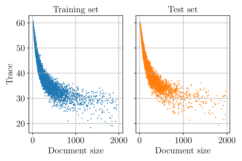
Figure 7: Uncertainty (trace of covariance of posterior distribution) captured in the document embeddings of 20Newsgroups dataset.

VIII Conclusions and future work

We have presented a generative model for learning document representations (embeddings) and their uncertainties. Our proposed model achieved state-of-the-art perplexity results on the standard 20Newsgroups and Fisher datasets. Next, we have shown that the proposed model is robust to over-fitting and unlike in SMM and NVDM, it does not require any early stopping mechanism for topic ID. We proposed an extension to simple Gaussian linear classifier that exploits the uncertainty in document embeddings and achieves better cross-entropy scores on the test data as compared to the simple GLC. Using simple linear classifiers on the obtained document embeddings, we achieved superior classification results on Fisher speech 20Newsgroups text corpora. We also addressed a commonly encountered problem of intractability while performing variational inference in mixed-logit models by using the re-parametrization trick. This idea can be translated in a straightforwardly for subspace $n$-gram model for learning sentence embeddings and also for learning word embeddings along with their uncertainties. The proposed Bayesian SMM can be extended to have topic-specific priors for document embeddings, which enables to encode topic label uncertainty explicitly in the document embeddings. There exists other scoring mechanisms that exploit the uncertainty in embeddings [46], which we plan to explore in our future works.

Appendix A Gradients of Lower Bound

The variational distribution is diagonal with the following parametrization:

$$q(\bm{w})=\mathcal{N}(\bm{w}\,|\,\bm{\nu},\mathrm{diag}(\exp\{2\bm{\varsigma}\})).$$ (43)

The lower bound for a single document is:

$$\mathcal{L}_{d}\approx-\frac{1}{2}\Bigg{[}\lambda\,\mathrm{tr}(\mathrm{diag}(\exp\{2\bm{\varsigma}\}))-\log|\mathrm{diag}(\exp\{2\bm{\varsigma}\})|\\ -K\,\log\lambda+\lambda\bm{\nu}^{{}^{\mkern-1.2mu\mathsf{T}}}\bm{\nu}-K\Bigg{]}\\ +\sum_{i=1}^{V}x_{i}\,\Bigg{[}\,(m_{i}+\bm{t}_{i}\bm{\nu})\\ \scalebox{0.75}[1.0]{$-$}\frac{1}{R}\sum_{r=1}^{R}\log(\sum_{j=1}^{V}\exp\{m_{j}+\bm{t}_{j}\,g(\bm{\epsilon}_{r})\})\Bigg{]},\\$$ (44)

where

$$g(\bm{\epsilon})=\bm{\nu}+\mathrm{diag}(\exp\{\bm{\varsigma}\}){\tilde{\bm{\epsilon}}}.$$ (45)

It is convenient to have the following derivatives:

$$\partialderivative{g({\bm{\epsilon}})}{{\bm{\nu}}} ={\bm{I}}.$$ (46)

$$\partialderivative{(\bm{t}_{i}g(\bm{\epsilon}))}{\bm{\varsigma}} =\mathrm{diag}(\bm{t}_{i}^{{}^{\mkern-1.2mu\mathsf{T}}})\,\mathrm{diag}(\exp\{\bm{\varsigma}\})\,\mathrm{diag}({\tilde{\bm{\epsilon}}})$$

$$=\bm{t}_{i}^{{}^{\mkern-1.2mu\mathsf{T}}}\odot\exp\{\bm{\varsigma}\}\odot{\tilde{\bm{\epsilon}}}.$$ (47)

Derivatives of the parameters of variational distribution:

Taking derivative of the objective function ((LABEL:eq:app_obj_baysmm)) with respect to mean parameter ${\bm{\nu}}$ and using (46):

$$\partialderivative{\mathcal{L}_{d}}{\bm{\nu}} =-\lambda\bm{\nu}+\sum_{i=1}^{V}x_{i}\Bigg{[}\bm{t}_{i}^{{}^{\mkern-1.2mu\mathsf{T}}}-$$

$${}\quad\frac{1}{R}\sum_{r=1}^{R}\sum_{k=1}^{V}\bm{t}_{k}^{{}^{\mkern-1.2mu\mathsf{T}}}{\bm{I}}\,\underbrace{\dfrac{\hfill\exp\{m_{k}+\bm{t}_{k}\,g(\bm{\epsilon}_{r})\}}{\sum_{j}\exp\{m_{j}+\bm{t}_{j}\,g(\bm{\epsilon}_{r})\}}}_{\theta_{kr}}\Bigg{]}$$ (48)

$$=\Big{[}\sum_{i=1}^{V}x_{i}\bm{t}_{i}^{{}^{\mkern-1.2mu\mathsf{T}}}-\sum_{i=1}^{V}\bm{t}_{i}^{{}^{\mkern-1.2mu\mathsf{T}}}\,\frac{1}{R}\sum_{r=1}^{R}\theta_{ir}\sum_{k=1}^{V}x_{k}\Big{]}-\lambda\bm{\nu}$$ (49)

$$\boxed{\nabla\bm{\nu}=\Big{[}\sum_{i=1}^{V}\bm{t}_{i}^{{}^{\mkern-1.2mu\mathsf{T}}}\big{(}x_{i}-\frac{1}{R}\sum_{r=1}^{R}\theta_{ir}\sum_{k=1}^{V}x_{k}\big{)}\Big{]}-\lambda\bm{\nu}.}$$ (50)

Taking the derivative of objective function ((LABEL:eq:app_obj_baysmm)) with respect to $\bm{\varsigma}$ and using (47):

$$\partialderivative{\mathcal{L}_{d}}{\bm{\varsigma}} =-\frac{1}{2}\Big{[}2\lambda\exp\{2\bm{\varsigma}\}-2\bm{I}\Big{]}$$

$${}+\sum_{i=1}^{V}x_{i}\Bigg{[}-\frac{1}{R}\sum_{r=1}^{R}\sum_{k=1}^{V}\bm{t}_{k}^{{}^{\mkern-1.2mu\mathsf{T}}}\bm{\epsilon}_{r}^{{}^{\mkern-1.2mu\mathsf{T}}}\underbrace{\dfrac{\hfill\exp\{m_{k}+\bm{t}_{k}g(\bm{\epsilon}_{r})\}}{\sum_{j}\exp\{m_{j}+\bm{t}_{j}g(\bm{\epsilon}_{r})\}}}_{\theta_{kr}}\Bigg{]}$$

$$=\bm{1}-\lambda\exp\{2\bm{\varsigma}\}$$

$$\qquad-\Big{[}\sum_{i=1}^{V}x_{i}\,\frac{1}{R}\sum_{r=1}^{R}\sum_{k=1}^{V}\bm{t}_{k}^{{}^{\mkern-1.2mu\mathsf{T}}}\odot\exp\{\bm{\varsigma}\}\odot{\tilde{\bm{\epsilon}}}_{r}^{{}^{\mkern-1.2mu\mathsf{T}}}\theta_{kr}\Big{]}$$ (51)

$$\nabla\bm{\varsigma} =\bm{1}-\lambda\exp\{2\bm{\varsigma}\}$$

$$\quad-\Bigg{[}\Big{(}\sum_{i=1}^{V}x_{i}\Big{)}\frac{1}{R}\sum_{r=1}^{R}\sum_{k=1}^{V}\theta_{kr}\bm{t}_{k}^{{}^{\mkern-1.2mu\mathsf{T}}}\odot\exp\{\bm{\varsigma}\}\odot{\tilde{\bm{\epsilon}}}_{r}\Bigg{]}.$$ (52)

Derivatives of the model parameters:

Taking the derivative of complete objective (17) with respect to a row ${\bm{t}}_{k}$ from matrix ${\bm{T}}$:

$$\partialderivative{\mathcal{L}}{\bm{t}_{k}} =\partialderivative{\bm{t}_{k}}\,\sum_{d=1}^{D}\sum_{i=1}^{V}x_{di}\Bigg{[}(m_{i}+\bm{t}_{i}\bm{\nu}_{d})$$

$$\qquad-\frac{1}{R}\sum_{r=1}^{R}\log(\sum_{j=1}^{V}\exp\{m_{j}+\bm{t}_{j}\,g(\,\bm{\epsilon}_{r}\,)\})\Bigg{]}$$

$$\qquad-\omega\sum_{i=1}^{V}\lvert\lvert\bm{t}_{i}\rvert\rvert_{1}$$ (53)

$$=\sum_{d=1}^{D}\Bigg{[}x_{dk}\bm{\nu}_{d}^{{}^{\mkern-1.2mu\mathsf{T}}}$$

$$\qquad-\sum_{i=1}^{V}x_{di}\frac{1}{R}\sum_{r=1}^{R}g(\bm{\epsilon}_{dr})^{{}^{\mkern-1.2mu\mathsf{T}}}\underbrace{\dfrac{\hfill\exp\{m_{i}+\bm{t}_{k}\,g(\bm{\epsilon}_{dr})\}}{\sum_{j}\exp\{m_{j}+\bm{t}_{j}g(\bm{\epsilon}_{dr})\}}}_{\theta_{dkr}}\Bigg{]}$$

$${}\qquad-\omega\,\mathrm{sign}(\bm{t}_{k})$$ (54)

$$=\sum_{d=1}^{D}\Bigg{[}x_{dk}\bm{\nu}_{d}^{{}^{\mkern-1.2mu\mathsf{T}}}-\sum_{i=1}^{V}x_{di}\frac{1}{R}\sum_{r=1}^{R}g(\bm{\epsilon}_{dr})^{{}^{\mkern-1.2mu\mathsf{T}}}\theta_{dkr}\Bigg{]}$$

$$\qquad-\omega\,\mathrm{sign}(\bm{t}_{k})$$ (55)

$${\nabla\bm{t}}_{k} =\sum_{d=1}^{D}\Bigg{[}x_{dk}\bm{\nu}_{d}^{{}^{\mkern-1.2mu\mathsf{T}}}-\Big{[}\Big{(}\sum_{i=1}^{V}x_{di}\Big{)}\frac{1}{R}\sum_{r=1}^{R}\theta_{dkr}g(\bm{\epsilon}_{dr})^{{}^{\mkern-1.2mu\mathsf{T}}}\Big{]}\Bigg{]}$$

$$\qquad-\omega\,\mathrm{sign}(\bm{t}_{k}).$$ (56)

Appendix B EM algorithm for GLCU

E-step:

Obtaining the posterior distribution of latent variable $p({\bm{y}}_{d}\,|\,{\bm{\nu}}_{d},\Theta)$. Using the results from [28] (p. 41, (358)):

$$\log p({\bm{y}}_{d}\, |\,{\bm{\nu}}_{d},{\bm{h}}_{d},\Theta)$$

$$=\log p(\bm{\nu}_{d}\mid\bm{y}_{d},\bm{h}_{d})+\log p(\bm{y}_{d})-\log p(\bm{\nu}_{d})$$

$$=\log\mathcal{N}(\bm{\nu}_{d}\mid\bm{\mu}_{d}+\bm{y}_{d},\bm{D}^{{}^{\mkern-1.2mu\mathsf{-1}}})$$

$${}\quad+\log\mathcal{N}(\bm{y}_{d}\mid\bm{0},\bm{\Gamma}_{d}^{{}^{\mkern-1.2mu\mathsf{-1}}})+\mathrm{const}$$

$$=-\frac{1}{2}(\bm{\nu}_{d}-(\bm{\mu}_{d}+\bm{y}_{d}))^{{}^{\mkern-1.2mu\mathsf{T}}}\bm{D}(\bm{\nu}_{d}-(\bm{\mu}_{d}+\bm{y}_{d}))$$

$${}\quad-\frac{1}{2}\bm{y}_{d}^{{}^{\mkern-1.2mu\mathsf{T}}}\bm{\Gamma}_{d}\bm{y}_{d}+\mathrm{const}$$

$$=-\frac{1}{2}(\bm{y}_{d}-(\bm{\nu}_{d}-\bm{\mu}_{d}))^{{}^{\mkern-1.2mu\mathsf{T}}}\bm{D}(\bm{y}_{d}-(\bm{\nu}_{d}-\bm{\mu}_{d}))$$

$${}\quad-\frac{1}{2}\bm{y}_{d}^{{}^{\mkern-1.2mu\mathsf{T}}}\bm{\Gamma}_{d}\bm{y}_{d}+\mathrm{const}$$

$$=\mathcal{N}(\bm{y}_{d}\mid\bm{u}_{d},\bm{V}_{d}^{{}^{\mkern-1.2mu\mathsf{-1}}})$$

where $${\bm{u}}_{d}$$ is simplified as:

$$\bm{u}_{d} =(\bm{D}+\bm{\Gamma}_{d})^{{}^{\mkern-1.2mu\mathsf{-1}}}(\bm{D}(\bm{\nu}_{d}-\bm{\mu}_{d})+\bm{\Gamma}_{d}\bm{0})$$

$$=[\bm{D}^{{}^{\mkern-1.2mu\mathsf{-1}}}(\bm{D}+\bm{\Gamma}_{d})]^{{}^{\mkern-1.2mu\mathsf{-1}}}(\bm{\nu}_{d}-\bm{\mu}_{d})$$

resulting in:

$$\bm{u}_{d} =[\bm{I}+\bm{D}^{{}^{\mkern-1.2mu\mathsf{-1}}}\bm{\Gamma}_{d}]^{{}^{\mkern-1.2mu\mathsf{-1}}}(\bm{\nu}_{d}-\bm{\mu}_{d})$$ (57)

$$\bm{V}_{d} =\bm{D}+\bm{\Gamma}_{d}$$ (58)

M-step:

Maximizing the auxiliary function

$$\Theta^{\textrm{new}} =\operatorname*{arg\,max}\limits_{\Theta}\,\mathcal{Q}(\Theta,\Theta^{\textrm{old}})$$ (59)

$$q(\bm{y}) =p(\bm{y}\mid\bm{w},\Theta^{\textrm{old}}).$$ (60)

Using the results from [28][p. 43, (378)], the auxiliary function $\mathcal{Q}(\Theta,\Theta^{\textrm{old}})$ is computed as:

$${}\mathcal{Q}(\Theta,\Theta^{\textrm{old}})$$

$$=\mathbb{E}_{q}[\sum_{d=1}^{D}\log p(\bm{\nu}_{d},\bm{y}_{d})]$$

$$=\sum_{d=1}^{D}\mathbb{E}_{q}[\log p(\bm{\nu}_{d}\mid\bm{y}_{d})]+\mathbb{E}_{q}[\log p(\bm{y}_{d})]$$

$$=\sum_{d=1}^{D}\mathbb{E}_{q}[\log\mathcal{N}(\bm{\nu}_{d}\mid\bm{\mu}_{d}+\bm{y}_{d},\bm{D}^{{}^{\mkern-1.2mu\mathsf{-1}}})]+\mathrm{const}$$

$$=\frac{D}{2}\log|\bm{D}|-\frac{1}{2}\sum_{d=1}^{D}\Big{[}\mathbb{E}_{q}[(\bm{\nu}_{d}-(\bm{\mu}_{d}+\bm{y}_{d}))^{{}^{\mkern-1.2mu\mathsf{T}}}\bm{D}$$

$${}\qquad\qquad(\bm{\nu}_{d}-(\bm{\mu}_{d}+\bm{y}_{d}))]\Big{]}+\mathrm{const}$$

$$=\frac{D}{2}\log|\bm{D}|-\frac{1}{2}\sum_{d=1}^{D}\Big{[}\mathrm{tr}(\bm{D}\bm{V}_{d}^{{}^{\mkern-1.2mu\mathsf{-1}}})$$

$${}\quad+(\bm{u}_{d}-(\bm{\nu}_{d}-\bm{\mu}_{d}))^{{}^{\mkern-1.2mu\mathsf{T}}}\bm{D}(\bm{u}_{d}-(\bm{\nu}_{d}-\bm{\mu}_{d}))\Big{]}$$

Maximizing the auxiliary function $\mathcal{Q}$ with respect to model parameters $\Theta=\{\bm{M},\bm{D}\}$

Taking derivative with respect to each column $${\bm{\mu}}_{\ell} {\bm{M}}$$ in and equating it to zero:

$$\partialderivative{\mathcal{Q}}{\bm{\mu}_{\ell}} =-\frac{1}{2}\partialderivative{\bm{\mu}_{\ell}}\sum_{d\in\mathcal{I}_{\ell}}\Big{[}(\bm{u}_{d}-(\bm{\nu}_{d}-\bm{\mu}_{\ell}))^{{}^{\mkern-1.2mu\mathsf{T}}}\bm{D}(\bm{u}_{d}-(\bm{\nu}_{d}-\bm{\mu}_{l}))\Big{]}$$ (61)

$$=-\frac{1}{2}\sum_{d\in\mathcal{I}_{\ell}}\,2\bm{D}\,\big{(}\bm{\mu}_{\ell}-(\bm{\nu}_{d}-\bm{u}_{d})\big{)}$$

$$=-\bm{D}\,\Big{(}\sum_{n\in\mathcal{I}_{\ell}}\,\bm{\mu}_{\ell}-\sum_{n\in\mathcal{I}_{\ell}}\,(\bm{\nu}_{d}-\bm{u}_{d})\Big{)}$$

$$\bm{\mu}_{\ell}=\frac{1}{|\mathcal{I}_{\ell}|}\sum_{n\in\mathcal{I}_{\ell}}(\bm{\nu}_{d}-\bm{u}_{d})$$ (62)

Taking derivative with respect to shared precision matrix ${\bm{D}}$ and equating it to zero:

$$\partialderivative{\mathcal{Q}}{\bm{D}} =\frac{D}{2}\bm{D}^{{}^{\mkern-1.2mu\mathsf{-1}}}-\frac{1}{2}\Big{(}\sum_{d=1}^{D}\bm{V}_{d}^{{}^{\mkern-1.2mu\mathsf{-1}}}\Big{)}^{{}^{\mkern-1.2mu\mathsf{T}}}$$

$$-\frac{1}{2}\Big{(}\sum_{d=1}^{D}(\bm{u}_{d}-(\bm{\nu}_{d}-\bm{\mu}_{d}))(\bm{u}_{d}-(\bm{\nu}_{d}-\bm{\mu}_{nl}))^{{}^{\mkern-1.2mu\mathsf{T}}}\Big{)}^{{}^{\mkern-1.2mu\mathsf{T}}}$$ (63)

$$\bm{D}^{{}^{\mkern-1.2mu\mathsf{-1}}} =\frac{1}{D}\Big{[}\sum_{d=1}^{D}\bm{V}_{d}^{{}^{\mkern-1.2mu\mathsf{-1}}}$$

$${}\quad+\sum_{d=1}^{D}(\bm{u}_{d}-(\bm{\nu}_{d}-\bm{\mu}_{nl}))(\bm{u}_{d}-(\bm{\nu}_{d}-\bm{\mu}_{d}))^{{}^{\mkern-1.2mu\mathsf{T}}}\Big{]}$$ (64)

References

- [1] X. Wei and W. B. Croft, “LDA-based document models for ad-hoc retrieval,” in Proc. of the 29th Annual International ACM SIGIR, August 2006, pp. 178–185.
- [2] T. Mikolov and G. Zweig, “Context dependent recurrent neural network language model,” in IEEE SLT Workshop, December 2012, pp. 234–239.
- [3] J. Wintrode and S. Khudanpur, “Limited resource term detection for effective topic identification of speech,” in IEEE ICASSP, May 2014, pp. 7118–7122.
- [4] X. Chen, T. Tan, X. Liu, P. Lanchantin, M. Wan, M. J. F. Gales, and P. C. Woodland, “Recurrent neural network language model adaptation for multi-genre broadcast speech recognition,” in Proc. Interspeech. ISCA, September 2015, pp. 3511–3515.
- [5] K. Beneš, S. Kesiraju, and L. Burget, “i-Vectors in Language Modeling: An Efficient Way of Domain Adaptation for Feed-Forward Models,” in Proc. Interspeech. ISCA, 2018, pp. 3383–3387.
- [6] T. Mikolov, I. Sutskever, K. Chen, G. S. Corrado, and J. Dean, “Distributed representations of words and phrases and their compositionality,” in Advances in NIPS, December 2013, pp. 3111–3119.
- [7] J. Pennington, R. Socher, and C. D. Manning, “GloVe: Global Vectors for Word Representation,” in Proc. of the 2014 Conference on EMNLP, ACL, October 2014, pp. 1532–1543.
- [8] Q. V. Le and T. Mikolov, “Distributed representations of sentences and documents,” in Proc. of the ICML, June 2014, pp. 1188–1196.
- [9] J. Howard and S. Ruder, “Universal Language Model Fine-tuning for Text Classification,” in Proc. of the 56th Annual Meeting of the ACL. Melbourne, Australia: ACL, Jul. 2018, pp. 328–339.
- [10] M. Peters, M. Neumann, M. Iyyer, M. Gardner, C. Clark, K. Lee, and L. Zettlemoyer, “Deep contextualized word representations,” in Proc. of the NAACL: HLT. ACL, Jun. 2018, pp. 2227–2237.
- [11] J. Devlin, M. Chang, K. Lee, and K. Toutanova, “BERT: Pre-training of Deep Bidirectional Transformers for Language Understanding,” CoRR, vol. abs/1810.04805v1, 2018.
- [12] C. Bishop, “Latent variable models,” in Learning in Graphical Models. MIT Press, January 1999, pp. 371–403.
- [13] D. M. Blei, “Probabilistic topic models,” Commun. ACM, vol. 55, no. 4, pp. 77–84, Apr. 2012.
- [14] D. P. Kingma and M. Welling, “Auto-Encoding Variational Bayes,” in Proc. of the 2nd ICLR, 2014.
- [15] Y. Miao, L. Yu, and P. Blunsom, “Neural variational inference for text processing,” in Proceedings of the 33rd ICML, ser. ICML’16. JMLR.org, 2016, pp. 1727–1736.
- [16] C. M. Bishop, Pattern Recognition and Machine Learning (Information Science and Statistics). Secaucus, NJ, USA: Springer-Verlag New York, Inc., 2006.
- [17] D. J. Rezende, S. Mohamed, and D. Wierstra, “Stochastic backpropagation and approximate inference in deep generative models,” in Proc. of the 31st ICML, ser. Proc. of Machine Learning Research, E. P. Xing and T. Jebara, Eds., vol. 32. Bejing, China: PMLR, 22–24 Jun 2014, pp. 1278–1286.
- [18] M. Soufifar, L. Burget, O. Plchot, S. Cumani, and J. Cernocký, “Regularized subspace n-gram model for phonotactic ivector extraction,” in INTERSPEECH. ISCA, Aug 2013, pp. 74–78.
- [19] C. May, F. Ferraro, A. McCree, J. Wintrode, D. Garcia-Romero, and B. V. Durme, “Topic identification and discovery on text and speech,” in Proc. of the 2015 Conference on EMNLP, September 2015, pp. 2377–2387.
- [20] S. Kesiraju, L. Burget, I. Szöke, and J. Černocký, “Learning Document Representations Using Subspace Multinomial Model,” in Proc. of INTERSPEECH. ISCA, September 2016, pp. 700–704.
- [21] D. M. Blei, A. Y. Ng, and M. I. Jordan, “Latent Dirichlet Allocation,” JMLR, vol. 3, pp. 993–1022, 2003.
- [22] D. M. Blei and J. D. Lafferty, “Correlated topic models,” in Advances in Neural Information Processing Systems NIPS, December 2005, pp. 147–154.
- [23] D. P. Kingma and J. Ba, “Adam: A method for stochastic optimization,” in 3rd ICLR, May 2015.
- [24] G. Andrew and J. Gao, “Scalable Training of L1-Regularized Log-Linear Models,” in Proc. of the 24th ICML. New York, USA: ACM, 2007, pp. 33–40.
- [25] M. Kockmann, L. Burget, O. Glembek, L. Ferrer, and J. Černocký, “Prosodic speaker verification using subspace multinomial models with intersession compensation,” in Proc. of INTERSPEECH. ISCA, September 2010, pp. 1061–1064.
- [26] N. Dehak, P. Kenny, R. Dehak, P. Dumouchel, and P. Ouellet, “Front-end factor analysis for speaker verification,” IEEE Trans. Audio, Speech & Language Processing, vol. 19, no. 4, pp. 788–798, 2011.
- [27] N. Depraetere and M. Vandebroek, “A comparison of variational approximations for fast inference in mixed logit models,” Computational Statistics, vol. 32, no. 1, pp. 93–125, 2017.
- [28] K. B. Petersen and M. S. Pedersen, “The Matrix Cookbook,” Nov 2012.
- [29] P. Kenny, T. Stafylakis, P. Ouellet, M. J. Alam, and P. Dumouchel, “PLDA for speaker verification with utterances of arbitrary duration,” in 2013 IEEE International Conference on Acoustics, Speech and Signal Processing, May 2013, pp. 7649–7653.
- [30] S. Cumani, O. Plchot, and R. Fér, “Exploiting i-vector posterior covariances for short-duration language recognition,” in Proc. of INTERSPEECH, no. 09. ISCA, 2015, pp. 1002–1006.
- [31] M. Soufifar, M. Kockmann, L. Burget et al., “iVector Approach to Phonotactic Language Recognition,” in Proc. of INTERSPEECH. ISCA, August 2011, pp. 2913–2916.
- [32] A. L. Maas, R. E. Daly, P. T. Pham, D. Huang, A. Y. Ng, and C. Potts, “Learning word vectors for sentiment analysis,” in The 49th Annual Meeting of the ACL: Human Language Technologies, June 2011, pp. 142–150.
- [33] J. Eisenstein, A. Ahmed, and E. P. Xing, “Sparse Additive Generative Models of Text,” in Proc. of the 28th ICML. USA: Omnipress, 2011, pp. 1041–1048.
- [34] M. V. S. Shashanka, B. Raj, and P. Smaragdis, “Sparse Overcomplete Latent Variable Decomposition of Counts Data,” in NIPS, December 2007, pp. 1313–1320.
- [35] J. Zhu and E. P. Xing, “Sparse Topical Coding,” in Proc. of the 27th Conference on UAI, July 2011, pp. 831–838.
- [36] D. Mekala, V. Gupta, B. Paranjape, and H. Karnick, “Scdv : Sparse composite document vectors using soft clustering over distributional representations,” in Proc. of the 2017 Conference on EMNLP. Copenhagen, Denmark: ACL, Sep. 2017, pp. 659–669.
- [37] T. J. Hazen, F. Richardson, and A. Margolis, “Topic Identification from Audio Recordings using Word and Phone Recognition Lattices,” in IEEE Workshop on ASRU, December 2007, pp. 659–664.
- [38] T. J. Hazen, “MCE Training Techniques for Topic Identification of Spoken Audio Documents,” IEEE Transactions on Audio, Speech, and Language Processing, vol. 19, no. 8, pp. 2451–2460, Nov 2011.
- [39] D. Povey, A. Ghoshal, G. Boulianne, L. Burget, O. Glembek, N. Goel, M. Hannemann, P. Motlicek, Y. Qian, P. Schwarz, J. Silovsky, G. Stemmer, and K. Vesely, “The Kaldi Speech Recognition Toolkit,” in IEEE Workshop on ASRU. IEEE Signal Processing Society, Dec 2011.
- [40] K. Veselý, A. Ghoshal, L. Burget, and D. Povey, “Sequence-discriminative training of deep neural networks,” in Proc. of INTERSPEECH. ISCA, August 2013, pp. 2345–2349.
- [41] N. Srivastava, R. Salakhutdinov, and G. Hinton, “Modeling documents with a deep boltzmann machine,” in Proc. of the Twenty-Ninth Conference on UAI, ser. UAI’13. Arlington, Virginia, United States: AUAI Press, 2013, pp. 616–624.
- [42] H. Larochelle and S. Lauly, “A neural autoregressive topic model,” in Advances in NIPS, December 2012, pp. 2717–2725.
- [43] A. Mnih and K. Gregor, “Neural variational inference and learning in belief networks,” in Proc. of the 31th ICML, June 2014, pp. 1791–1799.
- [44] R. Pappagari, J. Villalba, and N. Dehak, “Joint verification-identification in end-to-end multi-scale cnn framework for topic identification,” in IEEE ICASSP, April 2018, pp. 6199–6203.
- [45] P. Liu, X. Qiu, and X. Huang, “Learning context-sensitive word embeddings with neural tensor skip-gram model,” in Proc. of the 24th International Conference on Artificial Intelligence, ser. IJCAI’15. AAAI Press, 2015, pp. 1284–1290.
- [46] N. Brümmer, A. Silnova, L. Burget, and T. Stafylakis, “Gaussian meta-embeddings for efficient scoring of a heavy-tailed PLDA model,” in Proc. Odyssey 2018 The Speaker and Language Recognition Workshop, 2018, pp. 349–356.