Siblings, friends and acquaintances:
Testing galaxy association methods

Abstract

In order to constraint the limitations of association methods applied to galaxy surveys, we analysed the catalogue of halos at $z=0$ of a cosmological simulation, trying to reproduce the limitations that an observational survey deal with. We focused in the percolation method, usually called Friends of Friends method, commonly used in literature. The analysis was carried on the dark matter cosmological simulation MDPL2, from the Multidark project. Results point to a large fraction of contaminants for massive halos in high density environments. Thresholds in the association parameters and the subsequent analysis of observational properties can mitigate the occurrence of fake positives. The use of tests for substructures can also be efficient in particular cases.

1 Introduction

The evolution of the galaxies and their current observed properties are a consequence of the combined effects of self-regulated internal processes and external ones related with the environment where they lie. For instance, it is well established in literature that high density environments, like clusters of galaxies, present a larger fraction of early-type galaxies than the field (e.g. Baldry et al., 2006; Rasmussen et al., 2012; Finn et al., 2018), but the processes ruling this quenching are not clearly established and they have been subject of study in the last years (Kawinwanichakij et al., 2017). Several studies also point to differences in the properties of early-type galaxies depending on their environment, with field ellipticals having lower metallicities (Niemi et al., 2010; Lacerna et al., 2016), lighter halos (Méndez et al., 2009; Salinas et al., 2012; Richtler et al., 2015) and a larger proportion of intermediate-age mergers (Hernández-Toledo et al., 2008; Tal et al., 2009; Hirschmann et al., 2013) than those located in clusters. These topics demand a straight comparison between properties obtained from numerical simulations and observational surveys. This becomes more relevant with the new generation of numerical simulations (Vogelsberger et al., 2014; Schaye et al., 2015; Knebe et al., 2018), and the currently available galaxy surveys like Sloan Digital Sky Survey (SDSS York, 2000) or the 2MASS Extended Sources Calatogue (Skrutskie et al., 2006), and upcoming projects like the Large Synoptic Survey Telescope (LSST Ivezić et al., 2008).

Therefore, an accurate classification of the environments where the galaxies reside becomes a key point to understand its role in galaxy evolution. Several attempts to identify nearby groups and clusters of galaxies have been made in the past decades (e.g. de Vaucouleurs, 1975; Paturel, 1979), improving the accuracy of the methods through the development of algorithms based on objective methods like the linking-length percolation (Huchra & Geller, 1982), or the hierarchical clustering (Materne, 1978; Tully, 1988). These methods and similar ones derived from them have been widely applied to successive observational surveys that increased the number of galaxies in the local volume with more precise radial velocities measurements (e.g. Garcia, 1993; Crook et al., 2007; Makarov & Karachentsev, 2011). Global properties have proven to be consistent between several studies. For instance, Garcia (1993) applied a combination of percolation and hierarchical methods, finding that $\approx 42\%$ of the galaxies in the sample were clustered in groups of three or more members. Similar results were obtained by Makarov & Karachentsev (2011) using the percolation method ($\approx 45\%$). Nonetheless, Crook et al. (2007) applied the percolation method assuming two different sets of linking-length parameters, namely two density contrast levels, and the results assuming the low density contrast parameters double those for the high density ones ($\approx 59\%$ and $\approx 36\%$, respectively). This latter result points to the importance of the selection of parameters and the physical motivation for preferring certain values, which might lead to differing interpretations for the same group/cluster of galaxies (e.g. Caso et al., 2015; Hess et al., 2015). A more complex discussion emerges when we also consider the surroundings of clusters of galaxies as possible infalling regions (e.g. Kim et al., 2014), but this approach needs an extensive discussion about the definition of a cluster of galaxies, which exceeds the goals of the present study.

In several catalogues of nearby groups of galaxies based on redshift-space extragalactic databases authors have also analysed mock galaxy catalogues obtained from N-body simulations to test their results (e.g. Berlind et al., 2006; Robotham et al., 2011). In many cases, these analysis were included to determine the completeness of the group catalogues and/or the reliability of their detected members, but restricting their results by using specific sets of linking-length parameters and observational databases in each case. Eke et al. (2004a) applied a percolation method to the Two-Degree Field Galaxy Redshift Survey (2DFGRS), to test how the velocity dispersion and group sizes derived for the 2DFGRS are affected by variations in the algorithm parameters using a mock catalogue, and this analysis was extended to measure the impact of variations in the luminosity function (Eke et al., 2004b). Duarte & Mamon (2014) analysed the percolation method accuracy for different sets of linking-length parameters for a SDSS-like mock catalogue, created from the Millennium-II simulation (Boylan-Kolchin et al., 2009) and a semi-analytic model. Besides the completeness and completeness percentages, they obtained global values of fragmentation and merging for the true groups of galaxies, assuming luminosity and distance completeness with maximum redshift ranging from $z\approx 0.04$ to $z\approx 0.13$ for different luminosity limits (derived from the SDSS completeness). A similar approach was taken by Wojtak et al. (2018), comparing several association methods from recent studies, including percolation ones. They focused on the accuracy of dynamical mass estimations of galaxy clusters, using mock clusters from the Bolshoi cosmological simulation (Klypin et al., 2011) with masses above $10^{13}\,{\rm M_{\odot}}$. They found that all methods overestimate cluster masses when applied to contaminated samples, and underestimated them when the sample is incomplete, concluding that this might be the main source of the scatter in the mass scaling relation. Recently, Tempel et al. (2018) used the Multidark simulation (Klypin et al., 2016) to test contamination and completeness percentages for their galaxy association algorithm, based on Bayesian statistics. All these studies present relevant results in the testing of the accuracy of association methods, but they are focused on particular observational properties or observing catalogues. Hence, it is worth to perform an independent test of the association methods to understand their potential strengths, and how the limitations of observational astronomy can influence the measured properties of galaxy groups derived from the classification through the incidence of fake positives and/or lost members in the association.

In this work we analyse the percolation method by taking advantage of a large sample of galaxy halos extracted from a high resolution cosmological dark matter simulation to model the available data of observational surveys and test the method, focusing on the change in observational properties in the nearby Universe and possible constraints to improve the results. The paper is organised as follows. In Section 2 we describe the analysed simulation and the methods applied to assign magnitudes, velocities uncertainties and calculate the projected distances to build our simulated galaxy catalogue. Section 3 describes the analysed percolation method applied to the galaxy catalogue. Section 4 shows the criteria to select the linking length parameters, and the analysis of the results from the method, including possible constraints to improve the accuracy of the method. Finally, Section 5 summarises the results achieved in this work.

2 The sample

We analyse the MDPL2 cosmological dark matter simulation, which is part of the Multidark project (Klypin et al., 2016), and is publicly available through the official database of the project. This simulation consists in a periodic cubic volume of $1\,{\rm h^{-1}\,Gpc}$ of size length, filled with $3840^{3}$ particles with mass of $1.51\times 10^{9}\,{\rm h^{-1}\,M_{\odot}}$ and it considers the cosmological parameters of Planck Collaboration et al. (2013).

From the simulation we select the complete available catalogue of dark matter halos detected using Rockstar halo finder (Behroozi et al., 2013), specifically the ones corresponding to the local Universe ($z=0$). The catalogue is composed by main host halos found over the background density and satellite halos (or subhalos) lying within another halos. We consider each one of these structures as host of a unique galaxy, so the main halos become hosts of the central galaxies of each system, and the satellite halos are the hosts of the satellite galaxies. From each halo we extracted from the catalogue its position, velocity, host/satellite relationships and the mass and virial radius obtained considering a constant factor $\Delta=200$ with respect to the critical density of the Universe. Using this mass definition we restrict our selection to the halos with virial mass larger than $10^{11}\,\textrm{M}_{\odot}$. In order to obtain a collection of samples similar to the nearby Universe, we divided the simulation in smaller cubic volumes with $100\,{\rm h^{-1}\,Mpc}$ of side length, including an overlapped envelope of $10\,{\rm h^{-1}\,Mpc}$ of width to avoid biases at the edges of the volumes. Therefore, halos lying within these regions might be associated as subhalos by the methods applied in each volume, but they cannot trigger a new association as main halos.

To avoid numerically expensive projection calculations, the analysis is carried on in the three possible projection planes following the basis of the Cartesian comoving coordinates. Distances in the line-of-sight were used to obtain recessional velocities, assuming $H_{0}=67.77$ km s^-1 Mpc^-1.

2.1 Magnitudes allocation

In addition to the halo properties described in the previous section, we assigned to each halo a luminosity in the $K$ band by using a simple implementation of a halo occupation distribution method (HOD Vale & Ostriker, 2006; Conroy et al., 2006), which assigns each luminosity in a non parametric way. We simply assume a monotonic relation between the galaxy luminosities and the halo virial masses without making distinction between main hosts and satellites, by following

$$n_{\textrm{g}}(>L)=n_{\textrm{h}}(>M),$$ (1)

where $n_{\textrm{g}}$ and $n_{\textrm{h}}$ are the number density of galaxies and halos respectively. Whereas the halo number density is extracted directly from the simulation, the number density of galaxies must preserve the galaxy luminosity function (LF) which is modelled by the Schechter (1976) parametric function,

$$\frac{dn_{\textrm{g}}}{dL}=\frac{n_{*}}{L_{*}}\left(\frac{L}{L_{*}}\right)^{\alpha}\exp\left(-L/L_{*}\right).$$ (2)

In our model, we took the $K$–band luminosity function measured by Kochanek et al. (2001) from the 2MASS survey to assign $K$ magnitudes, which parameters are given by $K_{*}-5\log{\rm h}=-23.39\;\textrm{mag}$, $\alpha=-1.09$ and $n_{*}=1.16\times 10^{-2}\,{\rm h^{3}\,Mpc^{-3}}$. Expressing the Schechter LF in terms of the magnitudes and starting from the bright end of the distribution, rest frame $M_{K}$ magnitudes were assigned to all the halos using a precision of 0.01 mag. The most massive main halo in MDPL2 presents a virial mass of $\approx 2\times 10^{15}\,{\rm h^{-1}\,M_{\odot}}$, which is similar to the typical mass values derived for the Coma cluster in literature (e.g. Geller et al., 1999; Łokas & Mamon, 2003; Kubo et al., 2007). Hence, we choose the luminosity of NGC 4889, the brightest galaxy in the Coma cluster, as the upper limit for the HOD. If we assume $K=8.4$ mag (Gavazzi & Boselli, 1996) as the apparent magnitude and a distance of 94 Mpc (mean value for distance estimations from NED), its absolute magnitude in the $K$ filter is $M_{K}=-26.5$.

It is worth noting that this method does not make any distinction between the LFs of main hosts and satellites galaxies, introducing a bias in the assignation of magnitudes to the halos. Environmental effects acting on galaxies hosted on satellite halos influence their properties to evolve differently than those of the central galaxies. This produces a deviation from the assumed monotonic relation between the galaxy stellar mass and the halo dark matter mass. Nonetheless, the assigned magnitudes are only involved in the estimation of the radial velocities uncertainties, and these are large enough to mask any contribution due to the simplified treatment. Then, no effect is expected in the results of our analysis.

2.2 Velocities uncertainties

The uncertainties in radial velocity measurements ($eV_{\textrm{R}}$) are among the observational limitations we should take into account. In order to do this, we analyse $V_{\textrm{R}}$ measurements for a sample of galaxies obtained from the 2MASS Redshift Survey (Huchra et al., 2012), based on the Extended Sources Catalogue from 2MASS (Skrutskie et al., 2006). The Figure 1 shows $eV_{\textrm{R}}$ as a function of galaxy apparent magnitudes in $K$ filter. To obtain a phenomenological model of these measurements, the mean values were calculated using bins of 0.2 mag, which are depicted with open circles. A third-order polynomial was fitted to the data. The resulting curve is represented with the solid red line, while the green dashed lines show one standard deviation of the fit.

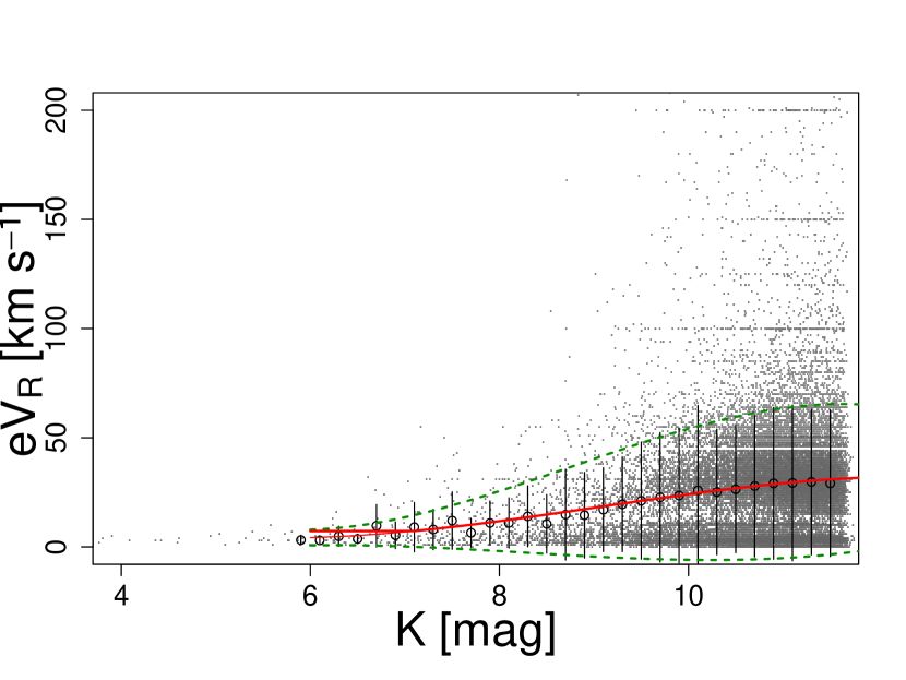
Figure 1: Uncertainties in radial velocity from the 2MASS Redshift Survey (Huchra et al., 2012) as a function of galaxies apparent magnitude in $K$ filter. Open circles show the mean values in bins of 0.2 mag, the solid red line represent a third-order polynomial fitted to data, while green dashed lines correspond to the standard deviation fit.

For each halo, its $K$ luminosity defines three apparent magnitudes, depending on the Cartesian plane chosen as projected sky plane. Hence, we added randomly generated uncertainties to the velocity components, assuming Gaussian distributions for the $eV_{\textrm{R}}$, with mean and standard deviation values are defined as functions of the $K$ apparent magnitude.

2.3 Projected distances

An important limitation in observational surveys of galaxies is the difficulty to measure accurate distances in the line-of-sight. This uncertainty propagates to the projected distances, resulting in a source of noise for the group finder methods. Following the criteria adopted by Crook et al. (2007), for each pair of halos we obtain projected distances from their projected angular separation ($\theta$, calculated from their comoving spatial coordinates) and the line-of-sight distance estimated from the average $V_{\textrm{R}}$. For the latter value there are two sources of uncertainty: the $eV_{\textrm{R}}$ modelled as it was described in the previous Section, and the halo peculiar velocities which might represent a significant fraction of the recessional velocity for nearby galaxies.

3 Linking-length percolation method

This family of methods, also called Friends of Friends methods, have been widely used for galaxy clustering in observational astronomy (e.g. Huchra & Geller, 1982; Garcia, 1993), but also for halo-finding in dark matter $N$-body simulations (e.g. Knebe et al., 2011, and references therein). In observational astronomy, the method proceed by linking a particular galaxy with all its neighbours that fulfil a set of criteria in projected distance and radial velocity, and the process is repeated with all the linked objects in an iterative process until no new galaxies are associated. The result is a unique system where a single member does not necessarily fulfil the criteria with all its partners, but it does it at least with a single one. In this work we follow the association algorithm described by Crook et al. (2007). This method presents two free parameters corresponding to the upper limits of the linking length in both radial velocities ($V_{\textrm{R,max}}$) and projected distances ($D_{\textrm{p,max}}$). To apply this method in the simulated catalogues, we consider two lower limits in virial mass, $10^{11}$ and $10^{12}\,\textrm{M}_{\odot}$, resulting in two different samples which are analysed independently.

In this paper, we do not go further on considerations about biases related to the completeness of the luminosity function for flux-limited surveys, neither completeness in redshift space. We assume the sample is complete up to the limiting virial mass at the entire redshift range, which roughly span up to $10^{4}$ km s^-1.

4 Results

4.1 Simulation statistics

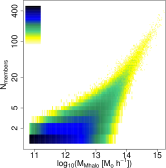
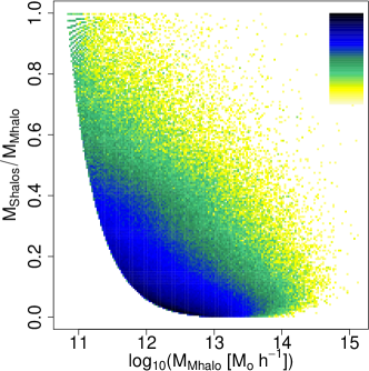
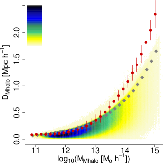
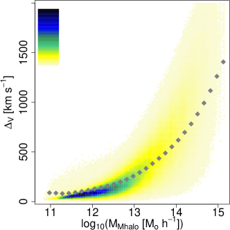
Figure 2: Distribution of different main halo properties as a function of their virial mass. In the four panels, the colour gradient ranges from yellow to black according to the value frequency. Upper-left panel: number of components in main halos, Upper-right panel: fraction of mass enclosed in satellite halos to main halo mass. Lower-left panel: spatial distance of satellite halos to the centre of the main halo. Grey diamonds indicate the mean virial radii ($R_{\textrm{vir}}$), red circles represent the mean distances of the farthest satellite halo ($D_{\max}$) and the error-bars their dispersion ($\sigma_{\textrm{D}}$). Lower-right panel: largest component in commovil velocities with respect to the main halo ($\Delta_{V,\max}$). Grey diamonds represent the mean of the largest component of the velocity dispersions ($\sigma_{V,\max}$) when we assume each satellite halo as a unique galaxy.

As a first approach, we test some general statistical properties of the halos resulting from the MDPL2 simulation which are relevant in the further analysis. These are shown in the Figure 2. The upper-left panel shows the distribution of the number of components in main halos. The y-axis is in logarithmic scale and the colour gradient gets darker towards more populated bins. Systems with at least ten components are typically more massive than $10^{13}\,{\rm M_{\odot}\,h^{-1}}$, whereas those with a hundred components present virial masses around a few times $10^{14}\,{\rm M_{\odot}\,h^{-1}}$. The most massive single halos present masses around $5\times 10^{13}\,{\rm M_{\odot}\,h^{-1}}$. The upper-right panel shows the fraction of mass contained in satellite halos, as a function of the main halo mass. While this fraction is lower than $0.5$ in the majority of the cases, and particularly in massive halos, in low mass halos it can reach larger values.

The lower-left panel in Figure 2 shows the distribution of spatial distances of subhalos to the corresponding main halo, in terms of main halo mass. Grey diamonds indicate the mean virial radii ($R_{\textrm{vir}}$), while red circles and their errorbars represent the mean distances of the farthest subhalo ($D_{\max}$) and their dispersion ($\sigma_{\textrm{D}}$), respectively. This latter parameter goes beyond the $R_{\textrm{vir}}$ for masses larger than $10^{13}\,{\rm M_{\odot}\,h^{-1}}$. For the most massive halos, $D_{\max}+\sigma_{\textrm{D}}$ reaches $\approx 1.5R_{\textrm{vir}}$.

The lower-right panel in Figure 2 shows the distribution of the largest component in peculiar velocities with respect to the corresponding main halo ($\Delta_{\textrm{V,max}}$) in terms of the main halo mass. Grey diamonds represent the mean of the largest component of the velocity dispersion for the system ($\sigma_{\textrm{V,max}}$), assuming each subhalo as a unique galaxy.

For comparison purposes, we calculate for each halo a numerical proxy to characterise the environmental density around it. This numerical density is defined as the number of detected halos having a physical distance lower than $1.75\,{\rm Mpc\,h^{-1}}$. This limiting radius represents the typical virial radius in the most massive main halos (see the third panel in Figure 2). This choice points to avoid biases that smaller radius might introduce in the numerical density of more populous systems.

4.2 Selection of linking length parameters

Crook et al. (2007) tested the variation in the percolation method when different parameter pairs were applied to a sample of nearby galaxy clusters. They found that the numbers of groups with three or more members was maximized for $V_{\textrm{R,max}}=399$ km s^-1 and $D_{\textrm{p,max}}=1.63$ Mpc. They also derived $V_{\textrm{R,max}}=350$ km s^-1 and $D_{\textrm{p,max}}=0.89$ Mpc as the parameters corresponding to a density contrast of $\delta\rho/\rho=80$, typical for groups of galaxies. As the lower-right panel of Figure 2 shows, the fraction of halos with $\Delta_{\textrm{V,max}}$ larger than these values of $V_{\textrm{R,max}}$ increases from $10^{12}\,{\rm M_{\odot}\,h^{-1}}$.

Taking advantage of the comprehensive knowledge of halos properties in the simulation, we proceed to compare the performance of the free parameters of the model by analysing the fraction of success in the allocation of satellite halos considering a mesh of values of the parameters. Assuming the association of halos in the simulation as the correct one, we define the fraction of success as the ratio of satellite halos correctly associated to their main halo to the total sample of satellite halos, in terms of their virial mass. In the Figure 3 we analyse the behaviour of this fraction by applying the percolation method for associating halos considering different sets of parameters. The values of these parameters ranged $D_{\textrm{p,max}}=0.1-2$ Mpc and $V_{\textrm{R,max}}=100-1600$ km s^-1. Smaller steps were adopted in regions with higher fraction of success to constrain the adopted parameters for further analysis. The colour gradients ranges from blue (low accuracy, $\approx 80\%$) to red (high accuracy, $\approx 95\%$). Although this range of accuracy seems quiet narrow, observational results derived under these conditions might differ significantly from the real values. In the following Sections we will go further on this. The upper panel in Figure 3 shows the results for the halos more massive than $10^{11}\,\textrm{M}_{\odot}$. The white curves represent the smoothed contour levels when only the main halos are considered in the calculation, ignoring satellites. This comparison allows us to emphasise the different behaviours related with changes in the linking length parameter. As expected, main halos tend to favour small values of $D_{\textrm{p,max}}$, with a weak dependence of the adopted $V_{\textrm{R,max}}$.

The lower panel is analogue to the previous one but applying the method in the sample of halos more massive than $10^{12}\,\textrm{M}_{\odot}$. Main halos with masses under this limit represent $\approx 87\%$ of the number of main halos but only $\approx 22\%$ of the virial mass. Their absence implies an increase in the mean distances between main halos and translates in wider ranges of $D_{\textrm{p,max}}$ for constant fractions of success.

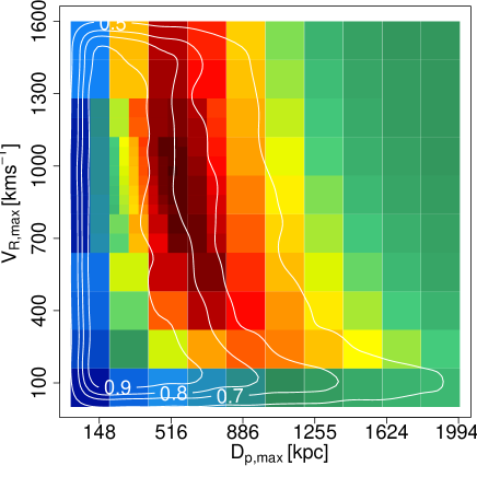
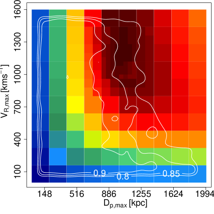
Figure 3: Ratio of satellite halos accurately associated to their main halo to the total sample of satellite halos in terms of the virial mass for different values of linking-length parameters in projected distance $D_{\textrm{p,max}}$ and radial velocity $V_{\textrm{R,max}}$. The colour gradients ranges from blue (low accuracy, $\approx 80\%$) to red (high accuracy, $\approx 95\%$). White curves indicate smoothed contour levels when main halos instead of satellite ones are taken into account. The upper and lower panels correspond to halos more massive than $10^{11}$ and $10^{12}\,\textrm{M}_{\odot}$, respectively.

In both cases, the behaviour of the fraction of success exhibit a strong dependence with the adopted value of $D_{\textrm{p,max}}$, whereas for $V_{\textrm{R,max}}$ there is a wide range of velocities which produce similar results. According to this, in both cases we manually select a definite set of parameters which maximises the fraction of success for both the main and satellite halos. Considering these selected values of the parameters and the original ones defined by Crook et al. (2007), we define three different cases to be analysed in more detail:

• Case (A) with $D_{\mathrm{p,max}}=525\,\mathrm{kpc}$ and $V_{\mathrm{R,max}}=980\,\mathrm{km\;s}^{-1}$. These give the best results for halos more massive than $10^{11}\,\textrm{M}_{\odot}$

• Case (B) with $D_{\mathrm{p,max}}=975\,\mathrm{kpc}$ and $V_{\mathrm{R,max}}=1100\,\mathrm{km\;s}^{-1}$. These give the best results for halos more massive than $10^{12}\,\textrm{M}_{\odot}$

• Case (C) with $D_{\mathrm{p,max}}=890\,\mathrm{kpc}$ and $V_{\mathrm{R,max}}=350\,\mathrm{km\;s}^{-1}$. These were defined by Crook et al. (2007), and we apply them to the sample of halos halos more massive than $10^{12}\,\textrm{M}_{\odot}$.

The choice of the more massive sample of halos for the case (C) is motivated on comparison purposes, considering that in the lower panel of Figure 3 these parameters show a low fraction of success for satellite halos, but a higher fraction for main halos than case (B).

It is worth noting that we repeated this analysis without considering the added noise in the radial velocities, resulting in no appreciable differences in the behaviour of the success fraction presented in the Figure 3.

In the following we highlight the main results from the percolation method. For simplicity, only results from a single projected plane are exposed. However the size of the sample avoid possible biases, which was tested from the comparison of the results in the three planes.

4.3 Method success and environmental density

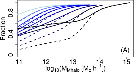
Figure 4: Fraction of halos (solid lines) and main halos (dashed lines) accurately classified by the method as a function of their main halo virial mass in case (A). The sample was split in several ranges of environmental density which are depicted with different line colours, so that darker colours represent denser environments.

To analyse the method success on the classification we quantify the number of halos that are accurately classified by the method with respect to the total. For this, we define as accurately classified halos to those assigned by the percolation method to the same system than the halo finder over the dark matter simulation. According to this, Figure 4 shows in solid lines the fraction of halos accurately classified by the method as a function of their main halo virial mass for the selection of halos more massive than $10^{11}\,{\rm M_{\odot}}$. The sample was split in percentiles of environmental density, so that line colours become darker towards denser environments. For instance, light blue corresponds to halos presenting at most a single neighbour closer than $1.75\,{\rm Mpch^{-1}}$, which represents $\approx 20\%$ of the halos, whereas the black line corresponds to the $5\%$ of halos located in the densest regions, typically cluster environments. The dashed lines correspond to main halos only, following the same density breaks than those applied to the general halo population. The cut off for low density percentiles responds to the absence of main halos more massive than a certain value.

These results indicate that the correct assignation of the halos has a strong dependence on the environment, with a large fraction of success for halos in low density ones. The accuracy get worse for main halos in denser environments, which are associated by the method to more massive halos close to them. The results for the general population of halos in these latter percentiles are noticeably better. This improvement is due to the selection of the linking-length parameters in Section 4.2 was optimised to accurately associate satellites to their main halos.

Figure 5 corresponds to the set of parameters analysed for halos more massive than $10^{12}\,{\rm M_{\odot}}$. The behaviour of the method is analogue to the case (A) in Figure 4, being less accurate for low mass main halos in denser environments. When we focus in main halos samples only, the results obtained in cases (B) and (C) differs significantly, as expected from their parameters chosen in Section 4.2.

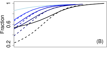
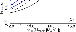
Figure 5: Same as in Figure 4, but for halos more massive than $10^{12}\,{\rm M_{\odot}}$ in cases (B) and (C).

Going forward with this analysis, we focus in the fate of halos wrongly classified by the method. Since the halo population is dominated by isolated low mass halos in the field or grouped in pairs (representing $\approx 93\%$ and $\approx 5\%$ of the main halos, respectively), we studied separately the sample of main halos presenting at least two satellites, assuming this as a simplistic threshold to define galaxy groups. We define $R_{\textrm{S/O}}$ as the ratio between the number of satellites originally defined by the halo finder over the dark matter simulation (S) and the number of halos associated by the method from the observable information (O). According to this, when $R_{\textrm{S/O}}>1$ the method associates too few halos as satellites, whereas when $R_{\textrm{S/O}}<1$ the method associates more satellites than the ones originally defined. Using this definition, Figure 6 shows the smoothed distribution of $R_{\textrm{S/O}}$ for the main halos having more than one satellite, as a function of the virial mass in case (A). The three panels correspond to density ranges with comparable number of halos, increasing from left to right. The colour bar ranges from yellow to black in the same manner than Figure 2, increasing for more probable values.

The distribution of ratios in the left panel looks somehow discretised in comparison with the other two panels. This is due to the low density of the environment where these main halos are located, particularly in main halos with few satellites and less neighbours. The method results successful in identifying the members of a larger number of main halos grouped around $R_{\textrm{S/O}}=1$, representing the $40\%$ of the main halos in this sample. Around $10\%$ of the main halos were associated to more massive ones, and for the $\approx 48\%$ the method associated a larger number of halos than their real satellites. There is a small fraction of halos with ratios larger than unity, indicating they were identified as main halos but lost some of their satellites. These halos typically present masses larger than $10^{12}\,{\rm M_{\odot}\,h^{-1}}$. On the other hand, the more massive main halos are able to achieve lower values of $R_{\textrm{S/O}}$. This might be due to the increase in the velocity dispersions of their real satellites, favouring the occurrence of fake positives.

The middle panel corresponds to intermediate environmental densities. The percentage of main halos with $R_{\textrm{S/O}}=1$ decreases ($\approx 18\%$) in favour of lower ratios ($\approx 63\%$). Also the fractions of main halos stripped of satellites or associated to more massive halos increase, representing the $14$ and $5\%$, respectively.

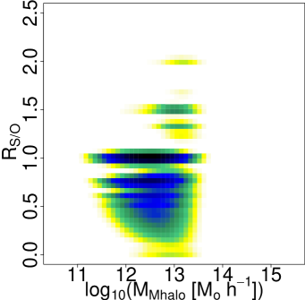
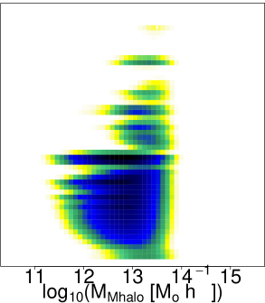
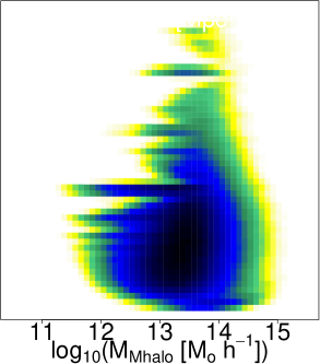
Figure 6: Smoothed distribution of the ratio between the number of satellites (S) and the number halos associated by the method from the observational constraints (O), $R_{S/O}$, for these main halos as a function of the virial mass in case (A). The three panels correspond to equally populated ranges of environmental density, increasing from left to right. The colour bar varies from yellow to black in the same manner as Figure 2, increasing for more probable values.

The right panel corresponds to the highest density environments, typical of rich groups and cluster of galaxies. The masses spans a wider range than previous panels, and the results point to a lack of accuracy in halos association. The behaviour of this sample continues the general trend of the previous panels, but with a marginal fraction of main halos around $R_{\textrm{S/O}}=1$ ($\approx 7\%$) and many cases of fake positives ($\approx 62\%$), with $\mu_{\textrm{R}}=0.5$ and $\sigma_{\textrm{R}}=0.22$ the mean and dispersion for main halos presenting $R_{\textrm{S/O}}<1$. The fraction of main halos stripped of their satellites decreases in favour of the halos associated to more massive main halos, representing the $7$ and $25\%$, respectively.

Figure 7 is analogue to the panel corresponding to the densest percentile in Figure 6, but for halos more massive than $10^{12}\,{\rm M_{\odot}\,h^{-1}}$ in cases (B) and (C), left and right panel, respectively. We do not include the panels corresponding to sparser environments to limit the number of figures. In both cases we found the same differences as in Figure 6.

In case (B) the distribution of main halos resembles the behaviour from Figure 6 (corresponding to case A). The distribution favour discrete values in sparser environments, presenting a large fraction of halos around $R_{\textrm{S/O}}=1$ which drops in denser regions from $54$ to $14\%$. On the other hand, main halos with $R_{\textrm{S/O}}<1$ rises from $36\%$ up to $62\%$ in cluster-like environments. The percentage of halos striped of satellites or that were associated to more massive main halos also increases with environmental density, remaining in all cases below $\approx 12\%$. These latter values are lower than those in case (A), indicating that the absence of the large number of halos with masses below $10^{12}\,{\rm M_{\odot}\,h^{-1}}$ makes more difficult the occurrence of fake positives.

The behaviour of the ratio differs for case (C) due to the different value of $V_{\textrm{R,max}}$, being 350 instead of 1100 km s^-1. This constrains the percentage of main halos with $R_{\textrm{S/O}}<1$ below $30\%$. Despite of this, there is no improvement in the fraction of main halos around $R_{\textrm{S/O}}=1$, which ranges from 44 to $12\%$, slightly smaller values than in case (B) and similar behaviour towards denser environments. The number of main halos accreted by more massive ones remains below $5\%$, but there is a large fraction of halos with lost satellites (i.e., $R_{\textrm{S/O}}>1$). This results are expected since the linking-length parameters chosen for case (C) favour the correct identification of main halos in detriment of satellites detection (see lower panel in Figure 3 and Section 4.2).

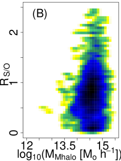
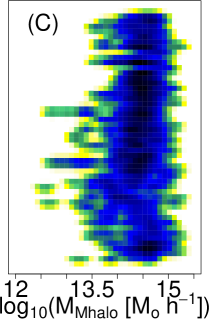
Figure 7: Smoothed distribution of the ratio between the number of satellites and the number halos associated by the method ($R_{\textrm{S/O}}$) for the densest percentile of halos more massive than $10^{12}\,{\rm M_{\odot}\,h^{-1}}$ in cases (B) and (C), left and right panels, respectively.

In Figures 6 and 7 we focused on main halos presenting at least two satellites because field halos and those with a single satellite dominate the population at low masses. Therefore, we now analyse the associations of the halos presenting less than two satellites.

The Figure 8 shows the distribution of the number of satellites associated by the method for different main halo masses and environmental densities. We split the sample in six mass bins and each one in three bins of increasing environmental density, with the first one corresponding to isolated galaxies, and the third one to the surroundings of a group/cluster of galaxies. The cuts to define the ranges of environmental density are chosen such that its bins are equally populated. The number of associated satellites is depicted with different colours, and in each bin they are organised in the y–axis according to the corresponding cumulative fraction with respect to the total. The upper panel of the figure corresponds to fields halos in case (A). Independently of the virial mass, the method is correctly classifying (those labelled with “0”) $\approx 70\%$ of the halos located in low density environments, with this fraction decreasing towards denser environments. Depending on the virial mass, misclassified halos will be associated to a more massive one (labelled with a dash in the plot) or will “acquire” fake satellites.

The lower panel of the Figure 8 is analogue to the upper one but only considering main halos with a single satellite. Once again, the method is more successful in low density environments, with slightly better results for intermediate mass halos. Except for the most massive bin, the number of halos classified as field ones is negligible. This occur because main halos with masses below few times $10^{13}\,{\rm M_{\odot}\,h^{-1}}$ present typical separations with their satellites in both projected distance and radial velocity smaller than $D_{\textrm{p,max}}$ and $V_{\textrm{R,max}}$, respectively (see middle-right and right panels in Figure 2). Hence, the chosen linking-length parameters restrict the association outcome of main halos and satellites. As expected, the most critical scenario takes place for halos in dense environments, with only $\approx 20\%$ of the cases being correctly classified.

The results when the analysed sample is restricted to halos more massive than $10^{12}\,{\rm M_{\odot}}$ varies depending on the linking-length parameters. The absence of halos in the mass range $10^{11}-10^{12}\,{\rm M_{\odot}}$ leads to larger mean distances for halos, driving to better results for larger $D_{\textrm{p,max}}$ (lower panel Figure 3). In case (B) the distribution presents a similar behaviour as in Figure 8, with minor changes in the percentages, for both field halos and those with a single satellite. In case (C) the fraction of properly classified field halos is larger and the typical number of fake satellites associated to massive halos is smaller. It also decreases the fraction of low mass main halos wrongly associated to more massive halos. For main halos presenting a single satellite results are also different in cases (B) and (C). In this latter case the method is successful for a larger fraction of main halos when their virial masses are lower than $10^{13}\,{\rm M_{\odot}\,h^{-1}}$, but it classifies as field halos a considerable fraction of halos above this limit. This is probably due to the restrictive value of $V_{\textrm{R,max}}$ considered in case (C).

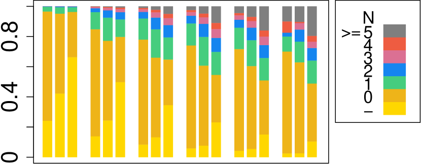
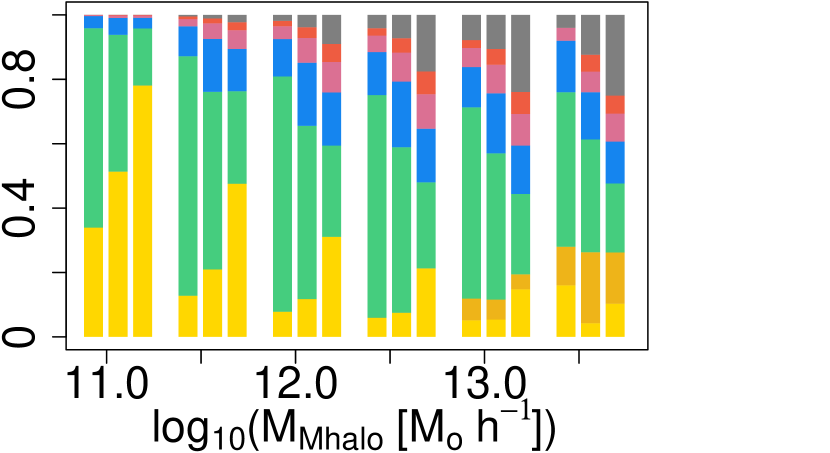
Figure 8: Distribution of the number of satellites associated by the method for field halos (upper panel) and halos with a single satellite (lower panel) in case (A). The samples are split in six bins of mass and each one in three density bins. The colour labelled with a dash correspond to halos associated by the method to more massive ones.

4.4 Comparing observational properties of real satellites and associated halos

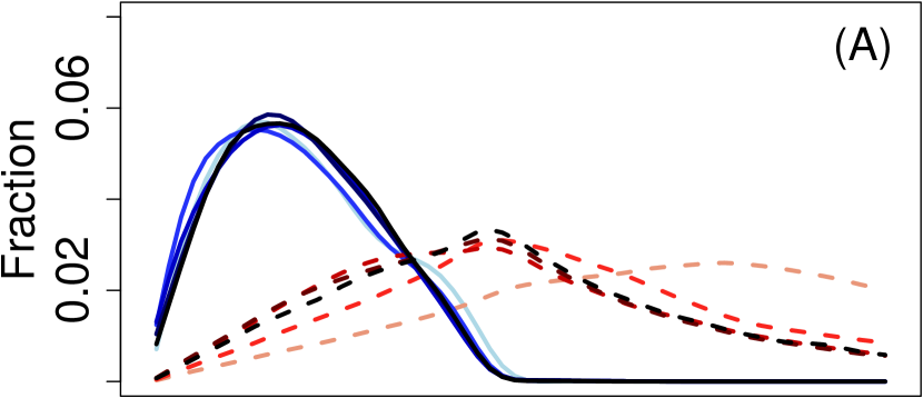
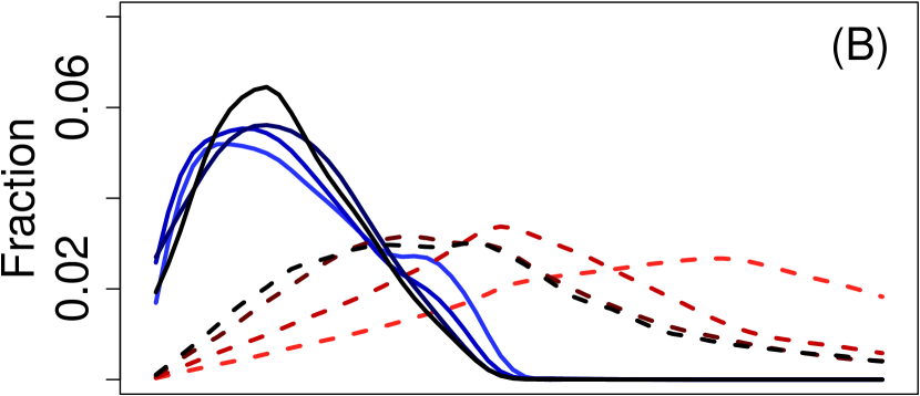
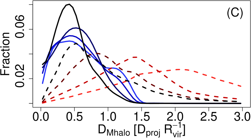
Figure 9: Distribution of projected distances to the main halo associated by the method for real satellites (solid lines) and fake positives (dashed lines). The gradient in colour scheme corresponds to mass intervals for the main halos, from the least (light) to the most massive ones (dark). The upper corresponds to the case of halos more massive than $10^{11}\,{\rm M_{\odot}}$, while middle and lower panels correspond to the two case analyzed for halos more massive than $10^{12}\,{\rm M_{\odot}}$.

Henceforth we analyse the impact on the derived observational properties of galaxies due to the method performance for the cases selected in Section 4.2. As a first approach, Figure 9 shows the distribution of projected distances to the main halo associated by the method for real satellites (solid lines) and fake positives (dashed lines). The gradient in colour corresponds to mass intervals for the main halos, from the least (lighter) to the most massive ones (darker). The projected distances are normalised by the virial radii, to facilitate the comparison between different mass intervals. In the three cases, most of the satellite distributions reach their upper limit at $R_{\rm proj}\approx 1.5R_{\rm vir}$, which is in agreement with the results from Section 4.1 and Figure 2.

The upper panel corresponds to results when the method is applied to halos more massive than $10^{11}\,{\rm M_{\odot}}$ (case A). In this case, the distributions of fake positives grow with the projected distance up to $R_{\rm proj}\approx 1.5R_{\rm vir}$, where distributions start to decline due the lack of “real” satellites to be associated with. The only exception is the distribution of the less massive main halos, which grows up to $\approx 3R_{\rm vir}$. This occurs because the mass interval spans virial masses in the range $\approx 10^{11}-10^{12}\,{\rm M_{\odot}\,h^{-1}}$, whose typical virial radii are much lower than the linking-length in projected distance $D_{\rm p,max}=525$ Mpc, i.e., $\approx 355\,{\rm Mpc\,h^{-1}}$.

A similar behaviour can be found in the middle panel, which corresponds to the case (B). In this case the linking-length is $\approx 660\,{\rm Mpc\,h^{-1}}$, comparable with the virial radius for a main halo of $\approx 5\times 10^{13}\,{\rm M_{\odot}\,h^{-1}}$. Likewise, the lower panel shows the results from case (C). The observed differences with the previous ones are a consequence of the more restrictive linking-length in radial velocities ($V_{\rm R,max}$) used in this case. For the most massive main halos, this choice translates in a lost of satellites in the outskirts (dark solid curve), resulting in a narrow distribution in comparison with case (B). This was already noticed in Figures 5 and 7. The choice of $V_{\rm R,max}$ also modified the distributions of fake positives, shifting the location of their maximum towards smaller projected distances (in terms of the virial radii).

The harmonic radius in groups of galaxies is associated with the spread in projected spatial distance between the members. The left panels in Figure 10 shows the ratio between the harmonic radius of galaxy groups associated by the method and the real harmonic radius of the groups, with this property as defined by Firth et al. (2006). As previously indicated, we consider the main halos with at least two satellite halos as a simplistic definition of galaxy groups. The sample is split in three bins of $R_{\rm S/O}$, presenting main halos largely contaminated ($R_{\rm S/O}<0.33$) with solid contour levels, moderately contaminated ($0.33<R_{\rm S/O}<0.66$) ones with dashed curves, and less contaminated main halos ($0.66<R_{\rm S/O}<1$) with dotted contour levels. The rows correspond to the three cases analysed in this paper. Those main halos largely contaminated show a wider distribution of ratios in cases (A) and (B), with the dotted distribution more concentrated towards ratio $\approx 1$. In case (C) the ratio of the harmonic radius for largely contaminated halos extend up to smaller values in comparison with case (B), due to the its more restrictive value of the linking-length $V_{\rm R,max}$, which is particularly important for massive main halos (see Figure 7). The right panels correspond to the ratio between the projected distances of the farthest halo associated by the method to that of the farthest real member, separated in bins of $R_{\rm S/O}$ in the same manner than in the other panels. This parameter exhibits a larger dispersion than the harmonic radius in all the cases, particularly in the cases of main halos largely contaminated.

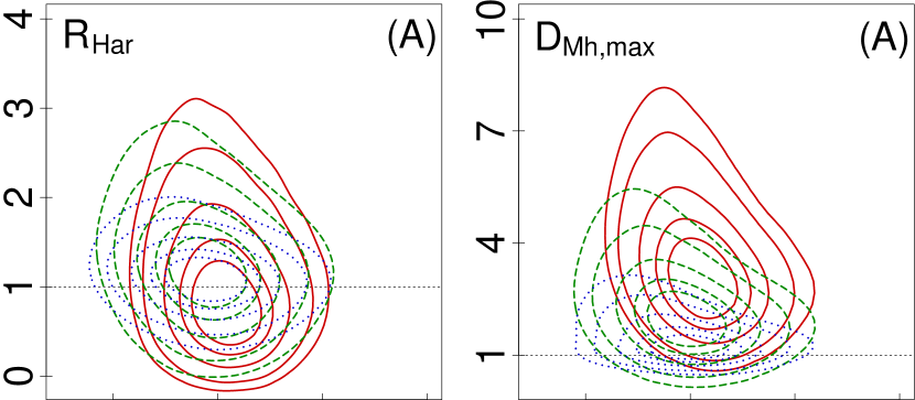
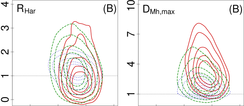
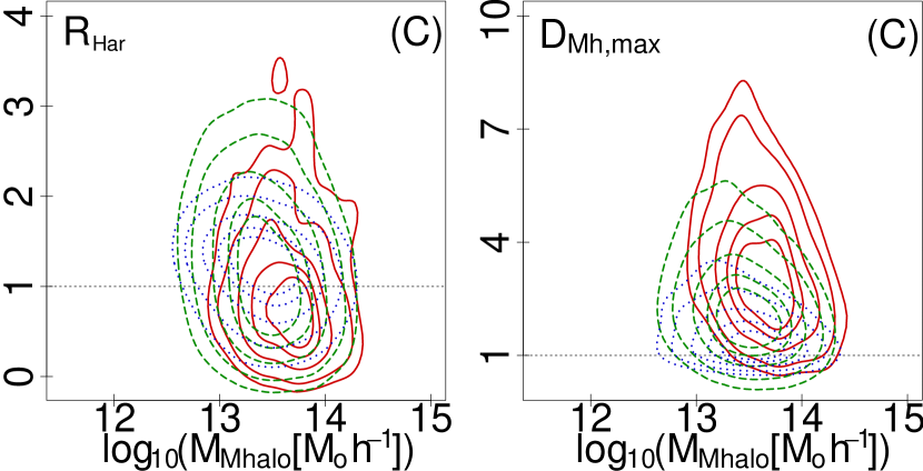
Figure 10: Left panels: Ratio between the harmonic radius associated by the method for galaxy groups, and their real harmonic radius, for the three cases analysed in this paper. Solid contour levels correspond to main halos with $R_{\rm S/O}<0.33$, dashed ones to $0.33<R_{\rm S/O}<0.66$, and dotted curves represent those with $0.66<R_{\rm S/O}<1$. Right panels: Ratio between the projected distances of the farthest halo associated by the method to that of the farthest real member, applying the same line code as previously indicated.

The distribution of radial velocities is useful to determine the probability of belonging to a group/cluster for galaxies with close projected distances. Nonetheless, the occurrence of fake positives in the association method can produce changes in the velocity dispersions observationally obtained for a main halo (i.e., “group/cluster of galaxies”) from their assumed members. Figure 11 shows the ratio between the velocity dispersion derived for halos associated by the method and their real velocity dispersion (R$\sigma_{\rm V_{x}}$) when halos more massive than $10^{11}\,{\rm M_{\odot}}$ are considered (i.e., case A). A value larger than one indicates the dispersion increases when we considered fake positives from the method. Its general distribution is depicted using filled coloured contours, where the darker ones represents the most populated levels. Moreover, we split the sample in three bins of $R_{\rm S/O}$ represented with different contour curves in the plot, considering main halos largely contaminated ($R_{\rm S/O}<0.33$, solid curves), moderately contaminated ($0.33<R_{\rm S/O}<0.66$, dashed curves) and less contaminated ($0.66<R_{\rm S/O}<1$, dotted curves). As expected, main halos largely contaminated show a wide and asymmetric distribution of ratios. The fraction of main halos with R$\sigma_{\rm V_{x}}>1$ decreases towards massive halos, reaching 0.5 at $\approx 10^{13}\,{\rm M_{\odot}\,h^{-1}}$. This mass roughly correspond to $\sigma_{\rm V_{x}}\approx 330$ km s^-1. Less massive main halos exhibit smaller dispersions, and the assumed linking-length $V_{\rm R,max}=980$ km s^-1 lead to an increase in the velocity dispersions due to fake associations of satellites. On the other hand, the majority of main halos at the massive end present R$\sigma_{\rm V_{x}}<1$.

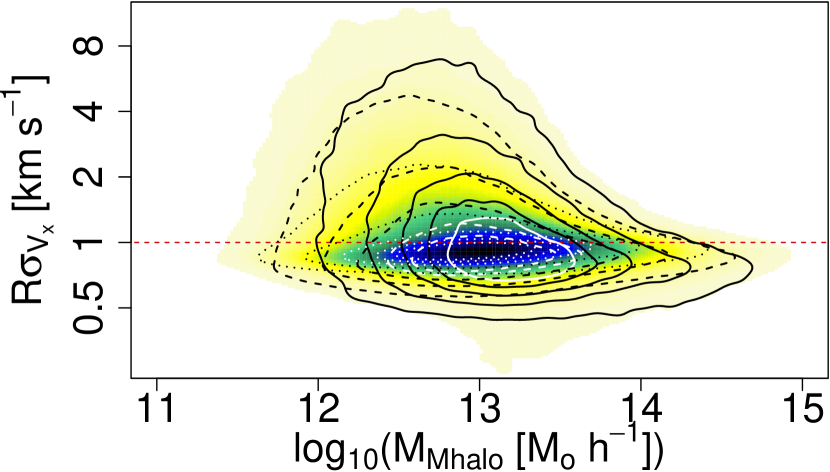
Figure 11: Distribution of the ratio between the velocity dispersion of main halos (R$\sigma_{\rm V_{x}}$) derived from halos associated by the method and the obtained from the real satellite halos, for the case (A), depicted with filled coloured contours. A value larger than 1 indicates the dispersion obtained from this latter halos is larger than the original. We also split the sample in three bins of $R_{\rm S/O}$ represented with different contour curves in the plot, considering main halos largely contaminated ($R_{\rm S/O}<0.33$, solid curves), moderately contaminated ($0.33<R_{\rm S/O}<0.66$, dashed curves) and less contaminated ($0.66<R_{\rm S/O}<1$, dotted curves).

Similar distributions are shown in Figure  12 for both linking-length choices when halos more massive than $10^{12}\,{\rm M_{\odot}}$ are considered. The behaviour is clearly different in cases (B) and (C), with this latter one presenting a bulk of main halos with R$\sigma_{\rm V_{x}}<1$ spread over a large range of masses. The sample was split in three bins in the same manner as Figure 11, and the contour curves follow the same prescription. Considering main halos ranging $0<R_{\rm S/O}<1$ do not describe the complete distribution in case (C), we added a fourth bin corresponding to $R_{\rm S/O}>1$ with dash–dotted lines. This is in agreement with the right panel of Figure 7, where a large number of main halos were located in this range, and it is responsible for the existence of this second bulk. The narrow linking-length assumed in case (C) lead to strip many satellites with large peculiar velocities from their main halos, with the subsequent decrease in the “observed” velocity dispersion.

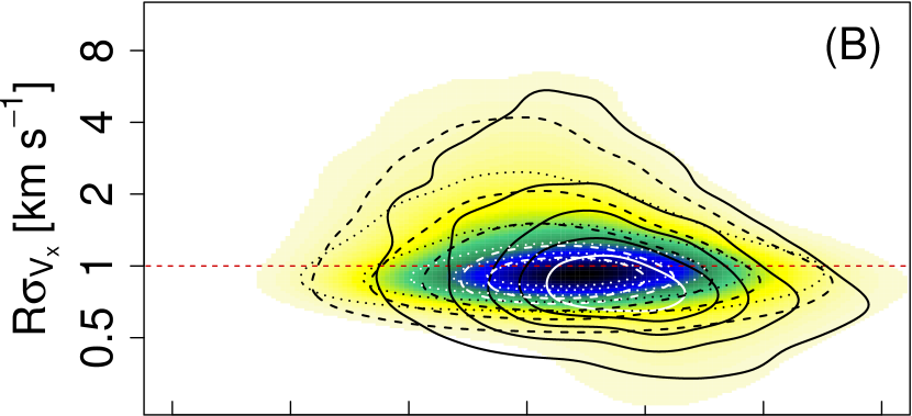
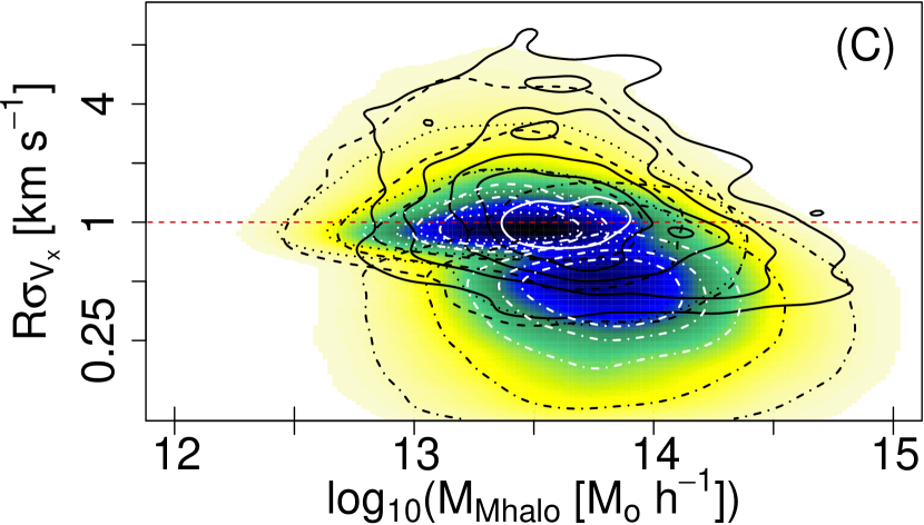
Figure 12: Distribution of velocity dispersion ratios, analogue to Figure 11 but for halos more massive than $10^{12}\,{\rm M_{\odot}}$ separating the cases (B) and (C). For this latter case, the main halos with $R_{\rm S/O}>1$ are also indicated in the diagram with dash–dotted contour curves.

The luminosity function is a well studied property in groups/clusters of galaxies (e.g. Schechter, 1976; Ricci et al., 2018, and references there in), having relevance as a constraint in numerical simulations of galaxy evolution (e.g. Gonzalez-Perez et al., 2014; Cora et al., 2018). In particular, the conditional luminosity functions of satellites and central galaxies are more affected by the association method, as halos incorrectly classified can highly contribute to the number counts of galaxies for main halos in specific virial mass ranges. The $K$ magnitude allocation described in Section 2.1 order the halos in terms of their virial masses without discrimination between field or satellite ones. Because galaxy evolution might depend on environmental factors, our luminosities are only indicative, and we do not pretend to directly compare results from this Section with observational neither numerical ones. However, the comparison between luminosity functions from real cluster members and halos associated by the method in this analysis is relevant to understand how dependent are observational results from the association of galaxies.

Figure 13 shows conditional luminosity functions for clusters of galaxies. These are obtained by selecting the main halos with virial masses larger than $10^{15}\,{\rm M_{\odot}\,h^{-1}}$ when the systems associations with the percolation method in the case (A) are considered (filled histograms), and they are compared with the clusters defined by the original simulation (solid thick line histograms). In both cases, the central galaxies (i.e, the luminosities assigned to the main halos) and satellites are presented separately with yellow and blue histograms, respectively. The luminosity function of central galaxies is significantly different in both cases, with a large contribution to lower luminosities of main halos achieving virial masses above $10^{15}\,{\rm M_{\odot}\,h^{-1}}$ when the method is applied. This behaviour is a consequence of the large number of fake satellites that are assigned by the method (these correspond typically to main halos with $R_{\rm S/O}<1$ in the right panel of Figure 6). Therefore, when results from the percolation method are assumed, the number of systems in this mass range is $\approx 4$ times larger than expected. These additional main halos constitute the population of galaxies that fills the fainter part of the distribution of luminosities. On the other hand, the number of satellites associated to these systems by the method is $\approx 7$ times larger, which implies that the number of satellite halos associated is $\approx 1.8$ times the mean number of satellites for main halos in this mass range. This overestimation of satellites contributes to the luminosity function homogeneously, since no difference is expected in the shape of the luminosity function for satellites with respect to the main halos virial mass.

Figure 13: Conditional luminosity functions of galaxies belonging to main halos with virial mass larger than $10^{15}\,{\rm M_{\odot}\,h^{-1}}$. Systems obtained from the percolation method in case (A) are shown in filled histograms, whereas the expected luminosity functions corresponding to the systems defined by the simulation are shown in solid thick lines histograms. Satellites and centrals are represented separately in blue and yellow histograms, respectively.

We repeated this analysis for decreasing virial mass ranges $10^{14}<M_{\rm vir}<10^{15}\,{\rm M_{\odot}\,h^{-1}}$ and $10^{13}<M_{\rm vir}<10^{14}\,{\rm M_{\odot}\,h^{-1}}$. The number of main halos in these mass ranges from the percolation method in terms of the real number of main halos decreases to $\approx 1.5$ and $\approx 1$, respectively. In both cases there is a paucity of main halos in the bright end of the distribution, and an excess of faint ones, both resulting from the contribution of fake satellites to the system virial mass. In these cases there also exist an overpopulation of satellites, which contributes homogeneously over the entire distributions, resulting $\approx 2.7$ and $\approx 2$ times the number of the originally bounded satellites, respectively. Hence, the mean excess of satellites per main halo are $\approx 1.8$ and $\approx 2$, respectively. This indicates an approximately steady mean fraction of fake positives for main halos more massive than $10^{13}\,{\rm M_{\odot}\,h^{-1}}$, which is in agreement with the distribution shown in the right panel of Figure 6.

On the other hand, results when halos more massive than $10^{12}\,{\rm M_{\odot}}$ are considered differ depending on the linking-length parameters (cases B and C). In case (B) we obtained a similar behaviour than previously indicated for case (A) for the three mass bins.

The restrictive choice for $V_{\rm R,max}$ for case (C) limits the identification of a significant portion of real satellites for massive main halos (right panel of Figure 7), comparable with massive clusters of galaxies, which present radial velocity dispersions in the order of several hundreds km s^-1. This is particularly striking for masses above $10^{15}\,{\rm M_{\odot}\,h^{-1}}$ whose conditional luminosity functions are presented in Figure 14. As it can be seen from the figure, it leads to a paucity of faint main halos and a shallower distribution for satellites, which result in ratios of $\approx 0.6$ and $\approx 0.3$, respectively. Therefore, the method only associates half the number of bounded satellites to halos more massive than $10^{15}\,{\rm M_{\odot}\,h^{-1}}$. This paucity is mitigated for halos in the bin $10^{14}<M_{\rm vir}<10^{15}\,{\rm M_{\odot}\,h^{-1}}$ and it is absent for the less massive bin where the ratios for main and satellite halos are $\approx 1$ and $\approx 1.5$, respectively, similar to those in cases (B) and (C).

Figure 14: Analogue to Figure 13 but considering halos more massive than $10^{12}\,{\rm M_{\odot}}$ (case C).

4.5 Dependence on approximations

To clarify previous analysis it is important to take into consideration how estimations ruled by observational limitations might affect the method. In this issue we point to the effect that velocity uncertainties and the estimation of projected distances might yield differences in the method results. Thus, we repeated the application of the method on our sample but considering two simplifications. First, to isolate the effect of the uncertainties in $V_{\rm R}$ we exclude them from the calculations. As simulated uncertainties depend on the apparent $K$ magnitude, we restricted this analysis to halos less massive than $10^{12}\,{\rm M_{\odot}\,h^{-1}}$, i.e. (fainter than $M_{K}=-23.1$ mag). We split the sample in three equally populated ranges of $V_{\rm R}$ and compared the fraction of accurately classified halos as a function of their virial mass. No significant changes were appreciated in the distributions, and the number of halos whose classification changed with respect to the original one was $\approx 1\%$ in the three cases, but with a lower fraction of success in the bin that corresponds to the lower $V_{\rm R}$ compared with the other ones. The negligible effect of this uncertainties in the overall analysis is expected due to the assumed values for the linking-length parameter $V_{\rm R,max}$. We must notice that the distribution of uncertainties assumed in Section 2.2 implies for a galaxy with $K=11$ mag $eV_{\rm R}=136\,{\rm km\,s^{-1}}$ at $3\sigma$ level.

To understand the different behaviour of the bin that corresponds to the lower $V_{\rm R}$, besides avoiding the uncertainties in $V_{\rm R}$, as a second approach we calculate the projected distances for each pair of halos from the real line-of-sight distance, instead of approaching it from the $V_{\rm R}$ mean (see Section 2.3). The sample was also split in three equally populated bins of $V_{\rm R}$. For neither the two furthest thirds, the comparison with the previous simplification results in no striking differences, with $\approx 3\%$ halos changing their classification. There was an improvement of performance for the nearest bin, achieving a similar fraction of accurately classified halos than the other bins, with $\approx 13\%$ of the halos changing their classification in comparison with the previous one. This points to the estimation of the line-of-sight distance as the main source of the discrepancy, due to the noise added by the relative peculiar velocity of the pair. This effect was mitigated for the other bins because the contribution from outflow velocities dominates the $V_{\rm R}$.

4.6 Constraints to the method

Even though our choices for linking-length parameters ensure a high fraction of success for both main and satellites halos, it is worth to go further with the analysis of typical projected distances.

From Figure 2 we concluded that the mean distance from the main halos centre to their furthest satellite ($D_{Mh,max}$) exceeds the typical virial radius for main halos more massive than $10^{13}\,{\rm M_{\odot}\,h^{-1}}$, evolving up to $\approx 1.4R_{\rm vir}$. Additionally, in the previous Section we noticed the differences in the distribution of projected distances to the main halo between real satellites and fake positives (Figure 9). For constraining the projected distances, we select as an upper limit the 95th percentile of $D_{Mh,max}$, which barely matches the $2\sigma$ deviation from the mean value of $D_{\rm Mh,max}$ across the entire mass range. The curve can be accurately approximated by the function

$${\rm D_{Mh,max}}(M)=\alpha\left(1+\frac{\beta(M-\gamma)}{\sqrt{1+\beta^{2}(M-\gamma)^{2}}}\right),$$ (3)

where $M$ corresponds to the $M_{\rm vir}$ of the main halo in logarithmic scale and units of ${\rm M_{\odot}\,h^{-1}}$, and ${\rm D_{Mh,max}}$ is in units of ${\rm Mpc\,h^{-1}}$. The fit of the function gives $\alpha=2.66\pm 0.11$, $\beta=-0.75\pm 0.01$ and $\gamma=14.93\pm 0.05$.

An equivalent analysis can be done for the radial velocity differences between the main halos and their satellites. We fitted the same function to the 95th percentile of ${\rm\Delta V_{R,max}}$ across the entire mass range, in units of ${\rm km\,s^{-1}}$. In this case, the parameters were $\alpha=1255\pm 19$, $\beta=-0.83\pm 0.01$ and $\gamma=14.03\pm 0.03$.

We rerun the percolation algorithm for halos more massive than $10^{11}\,{\rm M_{\odot}\,h^{-1}}$ (case A), applying the restrictions in the maximum projected distance to the main halo ($D_{\rm Mh,max}$) and the maximum difference in radial velocity (${\rm\Delta V_{R,max}}$). These restrictions resulted in an improvement in the fraction of halos accurately classified by the method. As an example, the upper panel of Figure 15 shows the evolution of the fraction of halos (solid curves) and main halos (dashed curves) accurately classified as a function of their main halo virial mass, for several ranges of environmental density. This is analogue to Figure 4, corresponding to case (A). The middle panel shows the ratio of the harmonic radius for halos associated by the method to halos gravitationally bounded in case (A), representing an improvement in comparison with the first row in Figure 10. The lower panel corresponds to the ratio of velocity dispersions, analogue to Figure 11. In this case the overall distribution follows the contour curves corresponding to the bin $0.66<R_{\rm S/O}<1$, pointing to the minor relevance of the other two bins.

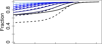
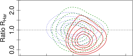
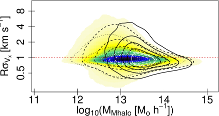
Figure 15: Upper panel: Fraction of halos (solid curves) and main halos (dashed curves) accurately classified as a function of their main halo virial mass, as in Figure 4 (case A). The sample was split in several ranges of environmental density, with colours becoming darker towards denser environments. Middle panel: Ratio between the harmonic radius (${\rm R_{Har}}$) of halos associated by the method and halos gravitationally bounded in case (A). The contour curves represent three bins of $R_{\rm S/O}$, as in Figure 10. Lower panel: Ratio between the velocity dispersion (R$\sigma_{\rm V_{x}}$) derived from halos associated by the method and real satellite halos, for the case (A). The colour gradient indicates the density distribution, and the contour curves represent three bins of $R_{\rm S/O}$, as in Figure 11.

In order to assess additional constraints, we also analysed the distribution of projected distances of satellite halos to their nearest neighbour (i.e., the nearest halo that belongs to the same main halo). We split the sample of main halos in five mass bins, each one equally populated of satellites halos. In each case, we rejected the cases which do not fulfil the linking-length criteria for $V_{\rm R}$. This is shown in the left panel of Figure 16 with different symbols. The labels refer to $M_{\rm vir}$ for the main halos in units of ${\rm M_{\odot}\,h^{-1}}$ and logarithmic scale. The distributions present a similar behaviour, becoming more disperse for more massive halos. The projected distance corresponding to the 95-percentile evolve from 240 kpc to 610 kpc from the less massive to the most massive bins, with marginal changes in the $D_{\rm near}$ distribution for main halos more massive than $10^{13}\,{\rm M_{\odot}\,h^{-1}}$. The latter values for the 95-percentile are barely larger than $D_{\rm p,max}=525$ kpc, the linking-length limit chosen in Section 4.2 for halos more massive than $10^{11}\,\textrm{M}_{\odot}$. A similar result is obtained when halos more massive than $10^{12}\,\textrm{M}_{\odot}$ are considered. Hence, this might be used to select an appropriate linking-length parameter $D_{\rm p,max}$ in observational studies.

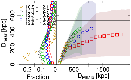
Figure 16: Left panel: Distribution of projected distances of satellite halos to their nearest neighbour, separated in five bins of mass equally populated. Right panel: change in the mean value of $D_{\rm near}$ for satellite halos, as a function of the distance to the centre of their main halo $D_{\rm Mhalo}$. Shaded regions represent the dispersion for each distribution.

The right panel of Figure 16 shows the change in the mean value of $D_{\rm near}$ for satellite halos, as a function of their projected distance to the centre of the corresponding main halo $D_{\rm Mhalo}$. The mass bins correspond to those indicated in the left panel, keeping the same symbol references. For main halos with masses below $10^{13}\,{\rm M_{\odot}\,h^{-1}}$ the change of $D_{\rm near}$ as a function of $D_{\rm Mhalo}$ does not depend on $M_{\rm vir}$. Instead, from that value it starts to become less steepy with increasing $M_{\rm vir}$. The filled regions indicate the ranges $D_{\rm near}$ spans within the 5th percentile lower and upper tails. The black solid line shows the linking-length parameter ($D_{\rm p,max}$) chosen in Section 3. The latter value is smaller than the 95th percentile for distances to the main halo comparable with the $R_{\rm Vir}$, but in Fig 9 it was found that the contribution of satellites at similar distances is minor, hence its 95th percentile is barely negligible. A similar result is obtained when only halos more massive than $10^{12}\,{\rm M_{\odot}\,h^{-1}}$ are considered. In this case, the typical number of satellites is lower, and the behaviour of $D_{\rm near}$ do not vary with the virial mass of the main halo. Then, no trend between the main halo virial mass and the typical value of $D_{\rm near}$, e.g. its 95th percentile, is evident for halos more massive than $10^{13}\,{\rm M_{\odot}\,h^{-1}}$. Similar results were obtained when the difference in radial velocities, ${\rm\Delta V_{R}}$, was taken into account. Then, we avoided to apply variable linking-length parameters.

From the results in previous Sections we can conclude that the method is less accurate for dense environments and low mass halos. This is particularly noticeable for main halos, due to the large number of field halos in the low mass regime. For instance, we selected from the simulation main halos in dense environments with more than ten satellites and virial masses from a few times $10^{13}$ to $10^{14}\,{\rm M_{\odot}}$, which correspond to the mass range of nearby clusters of galaxies like Fornax and Virgo. For those to whom the algorithm associated a larger number of halos than real satellites (corresponding to $\approx 70$ per cent of the total), the mean number of wrongly classified halos was $\approx 8.3$, with $\approx 81$ per cent of them being field halos and only $\approx 5$ per cent belonging to systems with more than five members. From these fake positives, $\approx 85$ per cent present masses below $10^{12}\,{\rm M_{\odot}}$. Consequently, the contribution to the virial mass of the main halo is negligible, but their inclusion might lead to inaccurate mass estimations due to variations in the dispersion of $V_{R\rm}$ (see Fig. 11).

We explored several options to identify main halos presenting a large fraction of fake positives, like Gaussian Mixture Model (Muratov & Gnedin, 2010) and nearest neighbours tests (Colless & Dunn, 1996), but the large fraction of fake positives corresponding to field halos blur structures in $V_{\rm R}$-space in the majority of the cases. A simplistic but efficient way to estimate the degree of contaminants in a cluster catalogue is to compare the distribution of projected distances to the main halo centre with the expected one, that presents a similar behaviour at all virial masses ranges when it is defined in terms of the main halo virial radius (see Figure 9). A particular case might be the analogue to a low-mass group classified by the method as part of a more massive cluster of galaxies. To present analogues to nearby clusters of galaxies, we selected again main halos in dense environments, with more than ten satellites and virial masses from a few times $10^{13}$ to $10^{14}\,{\rm M_{\odot}}$. We focused on those presenting at least five fake positives corresponding to the same main halo. We run the substructure test described in Colless & Dunn (1996) for the ten nearest neighbours. In this test the statistic is ruled by the probability of the K-S two-sample distribution (Kolmogorov, 1933; Smirnov, 1948), between each galaxy and its nearest neighbours, and the entire sample. The significance of the statistic is estimated by Monte Carlo simulations, in which the velocities of the galaxies are shuffled randomly. Hence, the zero hypothesis is that there is no substructure in the sample of galaxies. In a third of the main halos the presence of substructure cannot be ruled out at the 0.1 confidence level, and the proportion increases to nearly 50 per cent for the 0.2 confidence level. A control sample was chosen from the main halos in similar environments and mass range, but presenting a fraction of $R_{\rm S/O}$ from 0.9 to 1.1. From these, in 1 per cent of the cases the presence of substructure cannot be ruled out at the 0.1 confidence level. Hence, although the percolation algorithm results in an overpopulation of satellites for massive halos, subsequent analysis might improve the characterization.

In order to avoid adding noise from empirical fits and theoretical assumptions, the resulted fits were presented so far in terms of the halos virial mass instead of parameters like the stellar mass or the luminosity which might allow a direct comparison from observations. Despite of this, we are aware that observational surveys usually lack of accurate virial mass determinations due to the costs in telescope time of this type of analysis. Accurate constraints of mass-to-light ratios should be used to properly compare the results from the MDPL2 simulation with observational surveys, but this exceeds the goals from the present paper.

4.7 Implementation on observational data

Although the build-up of a group/clusters catalogue from observational surveys exceed the goals of this paper, it is worth testing the results with a sample of galaxies. We chose the surroundings of the Virgo cluster, because it has been extensively studied in the literature, including its substructure and satellite galaxies that might be falling in it.

The catalogue was obtained from the SDSS Data Release 7 (Abazajian et al., 2009), which has been used in previous studies focused on the Virgo cluster (Kim et al., 2014; Lisker et al., 2018). The chosen region spans $30\times 30$ deg², presenting galaxies that satisfy $172<RA<202$ deg and $-5<DE<25$ deg and ${\rm V_{R}<3000km\,s^{-1}}$, that includes the Virgo cluster and several groups of galaxies conforming the extended Virgo cluster catalogue (EVCC Kim et al., 2014, 2016). The SDSS spectroscopic survey covers galaxies brighter than $r\lesssim 17.77$, but bright and bulge-dominated galaxies were excluded due saturation problems. Hence, the catalogue was complemented with data from HyperLeda database (Makarov et al., 2014). The distance modulus for each galaxy was calculated from their radial velocities. This quantity was latter used to obtain absolute magnitudes in the $K$ filter. From the MDPL2 simulation we found that a halo with $10^{11}\,{\rm M_{\odot}}$ presents $M_{K}\approx-21$, then we used this magnitude as a selection limit for the sample of galaxies, resulting in 305 galaxies.

We applied the percolation method to the sample, using the linking length parameters calculated in Section 4.2 for the indicated mass limit corresponding to the case (A). The largest group of galaxies associated by the method might be identified with the main body of the Virgo cluster. This contains the giant ellipticals M 87 and M 49, as well as other 90 members (blue violet diamonds in Figure 17). Although it should be stressed that the use of radial velocities to estimate the distance in the line-of-sight leads to NGC 4501 as the most luminous galaxy of this association, instead of M 87. For instance, this approach estimates for NGC 4501 a distance modulus of $m_{M}\approx 32.6$, while SNIa measurements results in $m-M\approx 30.9$ (Mandel et al., 2011) and Tully-Fisher relations in $m-M\approx 31.5$ (Tully et al., 2013). Because redshift-independent measurements are not usually available in galaxy surveys, alternative estimations should be introduced in order to minimise these uncertainties.

The groups of galaxies typically called the W and M clouds were identified as independent associations to the Virgo cluster, which is supported by discussion about their stage of infall in literature (e.g. Binggeli et al., 1993; Gavazzi et al., 1999; Kim et al., 2014; Lisker et al., 2018). The percolation method also found the NGC 4636 group, a dinamically old group, lacking of late-type galaxies (Kim et al., 2014) and that exhibits intragroup X-ray emission that is distinct from the emission of the Virgo cluster (Brough et al., 2006).

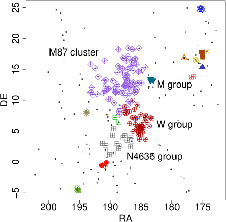
Figure 17: Results from applying the percolation method with the linking length parameters calculated in Section sec.param for a sample of galaxies brighter than $M_{K}=-21$ in the surroundings of the Virgo cluster. Different symbols correspond to associations of galaxies found by the method.

5 Summary

We applied a percolation method, commonly used in observational astronomy to identify groups and clusters, to the catalogue of halos corresponding to the local Universe ($z=0$) from the MDPL2 cosmological dark matter simulation. Two different cuts in halo mass were assumed in order to reproduce results for different completeness depths. We added noise to our incoming parameters, projected distances and radial velocities, looking to reproduce the limitations from an observational surveys. We summarizes our findings as follows:

• The method is less efficient in dense environments, presenting a large fraction of fake positives. The uncertainties in the incoming parameters are not responsible for the misclassified halos.

• The selection of the linking-length parameters is crucial for the success of the method. Because the number of satellite halos increases strongly with virial mass, the parameters that produce better results are defined by the most massive main halos.

• The linking-length parameter in projected distance depends strongly on the mass cut of the analysis, and it might be approximated by the 95-percentile of the distribution of projected distances to the closest neighbour in massive main halos.

• Observational properties derived from contaminated catalogues, like velocity dispersions or luminosity functions might deviate significantly from the accurate ones.

• Constraints to maximum projected distance and difference in radial velocities, in terms of the main halo virial mass, can contribute to significantly reduce fraction of misclassified halos.

• The analysis of the distribution of projected distances might be helpful to identify largely contaminated systems. The use of substructure tests can also provide information in particular cases.

• The method with the constraints derived in Section 4.6 was applied to a sample of galaxies in the surroundings of the Virgo cluster with halo masses above $10^{11}\,{\rm M_{\odot}}$. The groups identified by the method are in agreement with the results from the literature for this region.

References

- Abazajian et al. (2009) Abazajian K. N., et al., 2009, ApJS, 182, 543
- Baldry et al. (2006) Baldry I. K., Balogh M. L., Bower R. G., Glazebrook K., Nichol R. C., Bamford S. P., Budavari T., 2006, MNRAS, 373, 469
- Behroozi et al. (2013) Behroozi P. S., Wechsler R. H., Wu H.-Y., 2013, ApJ, 762, 109
- Berlind et al. (2006) Berlind A. A., et al., 2006, ApJS, 167, 1
- Binggeli et al. (1993) Binggeli B., Popescu C. C., Tammann G. A., 1993, A&AS, 98, 275
- Boylan-Kolchin et al. (2009) Boylan-Kolchin M., Springel V., White S. D. M., Jenkins A., Lemson G., 2009, MNRAS, 398, 1150
- Brough et al. (2006) Brough S., Forbes D. A., Kilborn V. A., Couch W., 2006, MNRAS, 370, 1223
- Caso et al. (2015) Caso J. P., Bassino L. P., Gómez M., 2015, MNRAS, 453, 4421
- Colless & Dunn (1996) Colless M., Dunn A. M., 1996, ApJ, 458, 435
- Conroy et al. (2006) Conroy C., Wechsler R. H., Kravtsov A. V., 2006, ApJ, 647, 201
- Cora et al. (2018) Cora S. A., et al., 2018, MNRAS, 479, 2
- Crook et al. (2007) Crook A. C., Huchra J. P., Martimbeau N., Masters K. L., Jarrett T., Macri L. M., 2007, ApJ, 655, 790
- Duarte & Mamon (2014) Duarte M., Mamon G. A., 2014, MNRAS, 440, 1763
- Eke et al. (2004a) Eke V. R., et al., 2004a, MNRAS, 348, 866
- Eke et al. (2004b) Eke V. R., et al., 2004b, MNRAS, 355, 769
- Finn et al. (2018) Finn R. A., et al., 2018, ApJ, 862, 149
- Firth et al. (2006) Firth P., Evstigneeva E. A., Jones J. B., Drinkwater M. J., Phillipps S., Gregg M. D., 2006, MNRAS, 372, 1856
- Garcia (1993) Garcia A. M., 1993, A&AS, 100, 47
- Gavazzi & Boselli (1996) Gavazzi G., Boselli A., 1996, Astrophysical Letters and Communications, 35, 1
- Gavazzi et al. (1999) Gavazzi G., Boselli A., Scodeggio M., Pierini D., Belsole E., 1999, MNRAS, 304, 595
- Geller et al. (1999) Geller M. J., Diaferio A., Kurtz M. J., 1999, ApJ, 517, L23
- Gonzalez-Perez et al. (2014) Gonzalez-Perez V., Lacey C. G., Baugh C. M., Lagos C. D. P., Helly J., Campbell D. J. R., Mitchell P. D., 2014, MNRAS, 439, 264
- Hernández-Toledo et al. (2008) Hernández-Toledo H. M., Vázquez-Mata J. A., Martínez-Vázquez L. A., Avila Reese V., Méndez-Hernández H., Ortega-Esbrí S., Núñez J. P. M., 2008, AJ, 136, 2115
- Hess et al. (2015) Hess K. M., Jarrett T. H., Carignan C., Passmoor S. S., Goedhart S., 2015, preprint, (arXiv:1506.06143)
- Hirschmann et al. (2013) Hirschmann M., De Lucia G., Iovino A., Cucciati O., 2013, MNRAS, 433, 1479
- Huchra & Geller (1982) Huchra J. P., Geller M. J., 1982, ApJ, 257, 423
- Huchra et al. (2012) Huchra J. P., et al., 2012, ApJS, 199, 26
- Ivezić et al. (2008) Ivezić Ž., et al., 2008, arXiv e-prints, p. arXiv:0805.2366
- Kawinwanichakij et al. (2017) Kawinwanichakij L., et al., 2017, ApJ, 847, 134
- Kim et al. (2014) Kim S., et al., 2014, ApJS, 215, 22
- Kim et al. (2016) Kim S., et al., 2016, ApJ, 833, 207
- Klypin et al. (2011) Klypin A. A., Trujillo-Gomez S., Primack J., 2011, ApJ, 740, 102
- Klypin et al. (2016) Klypin A., Yepes G., Gottlöber S., Prada F., Heb S., 2016, MNRAS, 457, 4340
- Knebe et al. (2011) Knebe A., et al., 2011, MNRAS, 415, 2293
- Knebe et al. (2018) Knebe A., et al., 2018, MNRAS, 474, 5206
- Kochanek et al. (2001) Kochanek C. S., et al., 2001, ApJ, 560, 566
- Kolmogorov (1933) Kolmogorov A., 1933, Giornale dell’Istituto Italiano degli Attuari, 4, 83
- Kubo et al. (2007) Kubo J. M., Stebbins A., Annis J., Dell’Antonio I. P., Lin H., Khiabanian H., Frieman J. A., 2007, ApJ, 671, 1466
- Lacerna et al. (2016) Lacerna I., Hernández-Toledo H. M., Avila-Reese V., Abonza-Sane J., del Olmo A., 2016, A&A, 588, A79
- Lisker et al. (2018) Lisker T., Vijayaraghavan R., Janz J., Gallagher III J. S., Engler C., Urich L., 2018, ApJ, 865, 40
- Łokas & Mamon (2003) Łokas E. L., Mamon G. A., 2003, MNRAS, 343, 401
- Makarov & Karachentsev (2011) Makarov D., Karachentsev I., 2011, MNRAS, 412, 2498
- Makarov et al. (2014) Makarov D., Prugniel P., Terekhova N., Courtois H., Vauglin I., 2014, A&A, 570, A13
- Mandel et al. (2011) Mandel K. S., Narayan G., Kirshner R. P., 2011, ApJ, 731, 120
- Materne (1978) Materne J., 1978, A&A, 63, 401
- Méndez et al. (2009) Méndez R. H., Teodorescu A. M., Kudritzki R.-P., Burkert A., 2009, ApJ, 691, 228
- Muratov & Gnedin (2010) Muratov A. L., Gnedin O. Y., 2010, ApJ, 718, 1266
- Niemi et al. (2010) Niemi S.-M., Heinämäki P., Nurmi P., Saar E., 2010, MNRAS, 405, 477
- Paturel (1979) Paturel G., 1979, A&A, 71, 106
- Planck Collaboration et al. (2013) Planck Collaboration et al., 2013, preprint, (arXiv:1303.5076)
- Rasmussen et al. (2012) Rasmussen J., Mulchaey J. S., Bai L., Ponman T. J., Raychaudhury S., Dariush A., 2012, ApJ, 757, 122
- Ricci et al. (2018) Ricci M., et al., 2018, A&A, 620, A13
- Richtler et al. (2015) Richtler T., Salinas R., Lane R. R., Hilker M., Schirmer M., 2015, A&A, 574, A21
- Robotham et al. (2011) Robotham A. S. G., et al., 2011, MNRAS, 416, 2640
- Salinas et al. (2012) Salinas R., Richtler T., Bassino L. P., Romanowsky A. J., Schuberth Y., 2012, A&A, 538, A87
- Schaye et al. (2015) Schaye J., et al., 2015, MNRAS, 446, 521
- Schechter (1976) Schechter P., 1976, ApJ, 203, 297
- Skrutskie et al. (2006) Skrutskie M. F., et al., 2006, AJ, 131, 1163
- Smirnov (1948) Smirnov N., 1948, The Annals of Mathematical Statistics, 19, 279
- Tal et al. (2009) Tal T., van Dokkum P. G., Nelan J., Bezanson R., 2009, AJ, 138, 1417
- Tempel et al. (2018) Tempel E., Kruuse M., Kipper R., Tuvikene T., Sorce J. G., Stoica R. S., 2018, A&A, 618, A81
- Tully (1988) Tully R. B., 1988, Nearby galaxies catalog
- Tully et al. (2013) Tully R. B., et al., 2013, AJ, 146, 86
- Vale & Ostriker (2006) Vale A., Ostriker J. P., 2006, MNRAS, 371, 1173
- Vogelsberger et al. (2014) Vogelsberger M., et al., 2014, MNRAS, 444, 1518
- Wojtak et al. (2018) Wojtak R., et al., 2018, MNRAS, 481, 324
- York (2000) York D. G. S., 2000, AJ, 120, 1579
- de Vaucouleurs (1975) de Vaucouleurs G., 1975, ApJ, 202, 610