Benadé and Hooker

Optimization Bounds from the Branching Dual

Optimization Bounds from the Branching Dual

J. G. Benadé, J. N. Hooker Carnegie Mellon University, jbenade@andrew.cmu.edu, jh38@andrew.cmu.edu

We present a general method for obtaining strong bounds for discrete optimization problems that is based on a concept of branching duality. It can be applied when no useful integer programming model is available, and we illustrate this with the minimum bandwidth problem. The method strengthens a known bound for a given problem by formulating a dual problem whose feasible solutions are partial branching trees. It solves the dual problem with a “worst-bound” local search heuristic that explores neighboring partial trees. After proving some optimality properties of the heuristic, we show that it substantially improves known combinatorial bounds for the minimum bandwidth problem with a modest amount of computation. It also obtains significantly tighter bounds than depth-first and breadth-first branching, demonstrating that the dual perspective can lead to better branching strategies when the object is to find valid bounds.

branching dual, dual bounds, minimum bandwidth

1 Introduction

Establishing bounds on the optimal value of a problem is an essential tool for combinatorial optimization. In a heuristic method, a good bound provides an indication of how close the solution is to optimality. In an exact algorithm, a known bound can allow one to prove optimality of a feasible solution found early in the search.

We propose a general method for obtaining optimization bounds that is based on the concept of a branching dual. It can, in particular, be applied to discrete optimization problems for which no useful integer programming models or cutting planes are available. It begins with a known bound, perhaps a weak one, and builds a branching tree that strengthens the bound as much as desired.

To obtain a good bound more quickly, we reconceive the branching process as local search in a dual space. We regard partial branching trees as dual solutions of the optimization problem and obtain neighboring solutions by adding branches to the tree. The value of a dual solution is defined to be the bound on the optimal value that is proved by the tree. If the objective of the primal problem is to minimize, the dual problem seeks to maximize this bound.

This results in a different kind of branching scheme than ordinarily used in methods that seek an optimal solution. Such methods typically attempt to solve both a primal and dual problem simultaneously. They branch in such a way as to find good feasible solutions, while simultaneously seeking to prove a tight bound on the optimal value. It is difficult to design a branching strategy that is effective at both tasks. We propose instead to focus on the dual problem by constructing trees that are specifically designed to discover good bounds.

The branching dual is clearly a strong dual, because a complete branching tree proves a bound equal to the optimal value. In practice, however, we seek a suboptimal solution of the dual that yields a good bound after a reasonable amount of computation. We do so by designing an effective local search procedure that takes advantage of problem structure. This affords an alternative perspective that may yield a bound more quickly than standard branching procedures.

The approach is somewhat similar to a Lagrangian method in which bounds are obtained by partially solving the Lagrangian dual, perhaps by subgradient optimization. Yet there are key differences. Because there is no duality gap, the branching dual can deliver a bound as tight as desired if we invest sufficient computational resources. Furthermore, there is no need for inequality constraints in the problem formulation (only inequality constraints can be dualized in a Lagrangian method), and no need to compute a subgradient or adjust the stepsize.

To solve the branching dual, we propose a worst-bound local search heuristic that examines neighboring solutions obtained by branching at nodes with the worst relaxation value. It is based on the principle that one should move to a neighboring solution that has some possibility of being better than the current solution.

We show that when the variable selected for branching at a node depends only on the node’s level in the tree (layered branching), the worst-bound heuristic is optimal in two senses. It obtains any desired bound with a tree of minimum size, and it obtains the tightest possible bound that can be obtained from a tree of a given size. In fact, these results hold more generally for fixed variable selection, which means that the choice of branching variable at a node depends only on the choices along the path from the root to the node.

When variable selection is not fixed, the heuristic examines neighboring solutions that result from various branching decisions. The search can be designed to exploit the characteristics of the problem at hand, much as is done with local search methods in general. We will see that a relatively simple local search procedure can substantially improve the bound.

The bound proved by a partial search tree is a function of the relaxation values computed at nodes of the tree. The relaxation value at a node is a bound on the value of any solution obtained in a subtree rooted at that node. If the problem has a tractable continuous relaxation, as in linear integer programming, we can obtain a relaxation value simply by fixing the variables on which the search has branched so far and solving the continuous relaxation that results. Relaxation values can often be obtained, however, without a continuous relaxation. If there is a known combinatorial bound for a given problem, we need only determine how to alter the bound to reflect the fact that certain variables have been fixed. This defines the relaxation values at nodes and allows a local search to improve the original bound, perhaps significantly.

We illustrate this strategy with the minimum bandwidth problem, for which no practical integer programming model is known. Bounds for this problem have been studied at least since 1970, when Chvátal introduced his famous density bound for the problem (Chvátal 1970). Since the density bound is NP-hard to compute, polynomially computable bounds have been proposed, such as those of Blum et al. (1998) and Caprara and Salazar-González (2005). We obtain relaxation values by adapting the Caprara–Salazar-González bound to the case where some variables are fixed.

We find in computational testing that the worst-bound heuristic delivers bounds that are not only better than the three bounds just mentioned, but that improve the Caprara–Salazar-González bound significantly faster than depth-first and breadth-first branching trees that use the same relaxation values. We obtain these results both with a layered branching order, where all the nodes on the same level branch on the same variable, and without. In fact, when variable selection does not only depend on the level a node is on, a straightforward local search heuristic can significantly improve the bounds. We conclude that the dual perspective proposed here can lead to better branching strategies when the object is to find valid bounds.

The paper is organized a follows. After a brief survey of related work, we define the branching dual and develop the idea of a relaxation function, which allows dual solutions to prove bounds on the optimal value. We then describe the worst-bound heuristic and show that it is optimal for fixed variable selection. The paper concludes with a computational study of the minimum bandwidth problem and remarks on future research.

2 Related work

A number of branching strategies have been proposed over the years, but almost always with the aim of solving a problem rather than obtaining a good dual bound quickly. Depth-first search immediately probes to the bottom of the tree and may therefore discover feasible solutions early in the search. It requires little space but tends to make slow progress toward improving the dual bound. Breadth-first search explores all the nodes on one level before moving to the next. It finds the best available bound down to the current depth but requires too much space for practical implementation.

Primal/dual node selection strategies attempt to obtain some of the advantages of both depth-first and breadth-first search. Iterative deepening (Korf 1985) conducts complete depth-first searches to successively greater depths, each time re-starting the search. It inherits the bound-proving capacity of breadth-first search while avoiding its exponential space requirement, but the amount of work still grows exponentially with the depth. Limited discrepancy search (Harvey and Ginsberg 1995) conducts a depth-first search in a band of nodes of gradually increasing width. Iteration 0 is a probe directly to the bottom of the tree. Iteration $k$ is a depth-first search in which at most $k$ variables are set to values different from those in iteration 0. This provides a bound at least as good as breadth-first search to level $k$, but the size of the search tree grows exponentially with $k$.

Cost-based branching uses relaxation values at nodes as a guide to branching. It is popular in mixed-integer solvers, where the relaxation values are obtained by solving (or estimating the solution value of) a continuous relaxation of the problem. The two basic strategies are worst-first and best-first node selection. Worst-first branching explores a node with the largest relaxation value first (if we are minimizing). Strong branching (Applegate et al. 2007, Bixby et al. 1995) might be viewed as similar to a worst-first strategy because it selects a branching variable that, when fixed, causes a large increase in the relaxation value. Pseudocosts (Benichou et al. 1971, Gautier and Ribier 1977) are often used instead of exact relaxation values to save computation time. Worst-first branching is slow to improve the dual bound, because it leaves nodes with small relaxation values open longer. This is of relatively little concern in branch-and-bound methods, because they use an upper bound and relaxation values at nodes (rather than the overall dual bound) to prune the search tree. However, worst-first branching is a poor strategy for quickly obtaining a good dual bound. Further discussion of these and related branching strategies can be found in Achterberg et al. (2005), Hooker (2012) and Linderoth and Savelsbergh (1999).

Best-first branching, by contrast, tends to improve the overall dual bound more quickly, because it explores nodes with the smallest relaxation value first. It is nondeterministic because there may be multiple nodes with the same relaxation value. It is shown in Achterberg (2007) that when variable selection is fixed, there exists a best-first node selection strategy that solves a given problem instance in a minimum number of nodes. This, of course, leaves open the question of which best-first strategy achieves this result. There is also the larger issue of which variable selection rule is best.

The worst-bound heuristic proposed here is based on the same idea as best-first branching but differs in that it simultaneously explores the children of all nodes with the smallest relaxation value. We call it “worst-bound” rather than “best-first” to reflect this difference and our emphasis on the dual bound. Because we are interested in bounding the optimal value rather than finding an optimal solution, we obtain somewhat stronger results than Achterberg (2007). Without assuming fixed variable selection, we show that for some selection of branching variables at nodes, the worst-bound heuristic proves any given valid bound with the minimum number of nodes. This does not tell us which variable selection rule is best, but the heuristic can conduct a local search to find a promising variable to branch on at a given node. Furthermore, we show that when the variable selection rule is fixed in advance, the worst-bound heuristic always proves a given bound with the minimum number of nodes, and it always proves the best bound that can be obtained by a tree with a given number of nodes.

We therefore build on Achterberg’s work in four ways: (a) we expand all relevant nodes with the minimum relaxation value, thus removing the non-determinism of best-first branching; (b) we prove the resulting algorithm is optimal for proving a dual bound; (c) we strengthen the algorithm with local search inspired by a concept of branching duality; and (d) we show empirically that the algorithm yields stronger dual bounds than depth-first and breadth-first branching.

Failure-directed search, recently proposed by Vilím et al. (2015) for scheduling problems, is similar to worst-bound branching in that it seeks to prove a bound (or infeasibility) rather than find a solution. However, the mechanism is quite different, because it makes branching “choices” that are most likely to lead to infeasibility, based on the structure of the scheduling problem. A “choice” is normally a higher-level decision, such as which currently unscheduled job to perform first. Orbital branching (Ostrowski et al. 2011) is designed for integer programming problems with a great deal of symmetry. Groups of equivalent variables are used to partition the feasible region, so as to reduce the effects of symmetry. It is unclear how these methods can be extended to a general branching method for optimization problems.

The idea of branching duality was introduced for purposes of sensitivity analysis in Hooker (1996) and Dawande and Hooker (2000). It is further developed in Hooker (2012), which suggests using a local search heuristic to solve the branching dual so as to obtain a bound on the optimal value. In the present paper, we carry out this suggestion by formulating a specific heuristic, proving its optimality properties, and applying it to the minimum bandwidth problem.

3 The Branching Dual

The branching dual is most naturally defined for a problem with finite-domain variables. We therefore consider an optimization problem of the form

$$\min\;\{f(x)\;|\;x\in F,\;x\in D\}$$ (1)

where $x=(x_{1},\ldots,x_{n})$, $F$ is the feasible set, $D=D_{x_{1}}\times\cdots\times D_{x_{n}}$, and each $D_{x_{j}}$ is the finite domain of variable $x_{j}$.

A (partial or complete) branching tree for (1) can be defined as follows. Let $T$ be a rooted tree, and for any node $u$ of $T$, let $P[u]$ be the path from the root to node $u$. We will say that $u$ is on level $j$ of $T$ when $P[u]$ contains $j-1$ arcs. A terminal node is any node on level $n+1$. Then $T$ is a branching tree if

(a) every nonterminal node $u$ is labeled with a variable $x_{j(u)}$ designating the variable being branched on at $u$, and the nodes in $P[u]$ have distinct labels;

(b) the arcs from any nonleaf node $u$ to its children are associated with distinct values in $x_{j(u)}$’s domain.

The value associated with an arc leaving $u$ is viewed as an assignment to $x_{j(u)}$. The arcs in $P[u]$ define a partial assignment $x[u]$ if $u$ is nonterminal and a complete assignment if $u$ is terminal.

Each branching tree $T$ establishes a lower bound $\theta(T)$ on the optimal value of (1), in a manner to be discussed in the next section. We will regard the tree $T$ as a dual solution of (1), and $\theta(T)$ as its value. The branching dual of (1) seeks a tree with maximum value:

$$\max\;\{\theta(T)\;|\;T\in\mathcal{T}\}$$ (2)

where $\mathcal{T}$ is the set of branching trees for (1). The branching dual maximizes the bound that can be obtained from a branching tree.

4 The Relaxation Function

To relate the structure of a tree $T$ to the bound $\theta(T)$, we suppose that each node $u$ of $T$ has a relaxation value $c_{u}$. This is a lower bound on the objective function value of any solution of (1) consistent with the partial assignment $x[u]$. We assume the following:

(a) The relaxation value is nondecreasing with tree depth, so that $c_{t}\leq c_{u}$ when $t$ is a parent of $u$.

(b) The relaxation value is a sharp bound at any terminal node $u$, meaning that $c_{u}$ is exactly the value of the corresponding assignment $x[u]$.

(c) The relaxation value is a function solely of the partial assignment $x[u]$, so that we can write $c_{u}=c(x[u])$, where $c(\cdot)$ is the relaxation function.

Condition (c) is useful because it implies that the relaxation value of $u$ does not change when nodes are added to the tree. This will allow us to prove various properties of the dual and algorithms for solving it.

Let an open node $u$ of $T$ be a nonterminal node at which branching is still possible; that is, $u$ has fewer than $|D_{x_{j(u)}}|$ children. A node that is not open is closed. Thus we have the following.

Lemma 4.1

A branching tree $T$ for (1) establishes a bound $\theta(T)$ equal to the minimum of $c_{u}$ over all terminal and open nodes $u$ in $T$.

The relaxation values can be obtained in any number of ways, so long as they satisfy (a)–(c). They can be values of a linear programming relaxation, perhaps strengthened with cutting planes, or they can reflect combinatorial bounds, as in the discussion of the minimum bandwidth problem to follow. They can also be strengthened by domain filtering and constraint propagation, as in constraint programming.

We will assume that any feasibility checks are encoded in the relaxation value, so that $c_{u}=\infty$ whenever infeasibility is detected at node $u$. We will say that $u$ is infeasible when $c_{u}=\infty$ and feasible when $c_{u}<\infty$. An infeasible node is more accurately called a provably infeasible node, but for brevity we will refer to it simply as an infeasible node.

The branching dual is a strong dual because $\theta(T)$ is the optimal value of (1) when $T$ is a complete branching tree. $T$ is complete when every node of $T$ is closed or infeasible.

Theorem 4.2

If $T$ is a complete branching tree for (1), then $\theta(T)$ is the optimal value of (1).

Proof. Suppose first that (1) is feasible, and let $x^{*}$ be an optimal solution. Let $P[u]$ be a longest path in $T$ for which $x[u]$ is consistent with $x^{*}$. Suppose $u$ is nonterminal. If $u$ is closed, some arc leaving $u$ assigns $x^{*}_{j(u)}$ to $x_{j(u)}$, which is impossible because $P[u]$ has maximal length. Also $u$ cannot be infeasible, because $x^{*}$ is feasible. Therefore, $u$ is terminal, which implies $c_{u}=\theta(T)=f(x^{*})$. If (1) is infeasible and thus has value $\infty$, any terminal node of $T$ must be infeasible. Since any open node is infeasible, Lemma 4.1 implies that $\theta(T)=\infty$. $\Box$

Corollary 4.3

The branching dual is a strong dual.

5 Solving the Dual

The branching dual can be solved by a local search algorithm that moves from the current solution to a neighboring solution. In general, a neighbor of $T$ could be any tree obtained by adding children to open nodes and/or removing leaf nodes. We will suppose that the algorithm only adds nodes and does not remove them, because this prevents cycling and ensures that the number of iterations is bounded by the number of possible nodes. In addition, the monotonicity of the relaxation function implies that the resulting dual values are nondecreasing. Because there is no cycling, uphill search eventually finds an optimal solution. This can still be regarded as local search in the sense that it searches a neighborhood of the current solution in each iteration.

It remains to specify which nodes to add in each iteration. Recall that the value of the current dual solution is governed by the worst (smallest) relaxation value of an open or terminal node $u$. If $u$ is terminal, the heuristic terminates with the optimal bound $c_{u}$. Otherwise, we propose adding nodes that can actually improve the current bound. Expanding a node with a relaxation value better than the worst cannot improve the bound, because it leaves open nodes with relaxation values equal to the current bound. However, expanding all nodes with the worst relaxation value can improve the bound. We will refer to this as a worst-bound heuristic.

The heuristic is stated more precisely in Algorithm 1, in which $T$ is the current dual solution. An eligible node is an open node $u$ with relaxation value $c_{u}=\theta(T)$. Note that every dual solution created by the heuristic is a saturated tree, meaning that all of its nonleaf nodes are closed.

Let $T$ initially consist of the root node;

while some open or terminal node in $T$ is feasible do

       if some terminal node $u$ in $T$ has relaxation value $c_{u}=\theta(T)$ then

             stop with the optimal bound $\theta(T)$;

            

      else

             for each eligible node $u$ in $T$ do

                   select a label $x_{j(u)}$ for $u$ that does not occur in path $P[u]$;

                   add to $T$ all children of $u$ to create the next dual solution;

                  

             end for

            

       end if

      

end while

problem (1) is infeasible;

Algorithm 1 Worst-bound heuristic

The heuristic must somehow specify how to select a label for each eligible node $u$. The labels are predetermined if variable selection is fixed, because in this case, the label at a node $u$ is a function of the labels on the other nodes along the path $P[u]$. As an example, Fig. 1 shows how the worst-bound heuristic may proceed when variable selection is not only fixed, but branching is layered (i.e., each node on level $j$ receives label $x_{j}$).

Figure 1: Three iterations of the worst-bound heuristic for a layered variable ordering. Each node is inscribed with its relaxation value. All variables are binary: a solid arc indicates assigning the value 1, a dashed arc 0. The shaded nodes will be examined in the next iteration.

If variable section is not fixed, a local search is conducted to select labels for eligible nodes. A greedy heuristic is the simplest approach, and we use it here. For each eligible node $u$, examine a subset of the variables that are available to label $u$, and select one that will maximize the minimum relaxation value of $u$’s children. The subset of variables considered depends on the characteristics of the problem at hand. Naturally, if the subset selected depends only on $P[u]$, the local search simply defines a fixed variable selection rule. However, if the subset is random or depends on factors other than $P[u]$, then variable selection is not fixed. Even if the local search yields a fixed selection rule, a rule obtained at runtime may be better than one determined a priori. We will find that this is in fact the case. In addition, the worst-bound heuristic is optimal for a branching rule obtained at runtime when it is a fixed selection rule.

The worst-bound heuristic is polynomial in the number of possible nodes, because the number of iterations is bounded by the number of nodes, and each iteration requires, at worst, examining each node of the current tree, and for each node, the children that result from selecting each possible label.

6 Properties of the Worst-Bound Heuristic

If variable selection is fixed, the worst-bound heuristic is optimal in two senses: it finds the smallest branching tree that yields a given bound, and it finds the tightest possible bound that can be obtained from a tree of a given size. We first establish a general result that holds even when there is no fixed variable selection. We will say that branching tree $T^{\prime}$ is a branching subtree of branching tree $T$ if $T^{\prime}$ is a subtree of $T$ and the node labels in $T^{\prime}$ are the same as in $T$.

Theorem 6.1

Given any branching tree $T$ for (1) that establishes a bound $\lambda$, the worst-bound heuristic can be executed in such a way as to create a branching subtree of $T$ that establishes the same bound $\lambda$.

Proof. We wish to show that the worst-bound heuristic can construct a branching subtree $T^{\prime}$ of $T$ that establishes the bound $\lambda$. We do so by first removing nodes from $T$ in a particular order until only the root node remains, and then constructing $T^{\prime}$ by showing that the worst-first heuristic restores removed nodes in reverse order until $\lambda$ is proved. We denote by $\lambda_{1},\ldots,\lambda_{k}$ the distinct relaxation values of the nodes of $T$ that are less than or equal to $\lambda$, where $\lambda_{k}=\lambda$ and $\lambda_{1}<\cdots<\lambda_{k}$. We next clean up $T$ by removing all leaf nodes whose parents have relaxation value of $\lambda_{k}$ or higher, and repeating until no such leaf nodes remain. This yields a branching subtree $T_{k}$ of $T$ that still establishes bound $\lambda_{k}$. Furthermore, $T_{k}$ is saturated, because if it contained an open nonleaf node $u$, then either $c_{u}<\lambda_{k}$ or $c_{u}\geq\lambda_{k}$. In the former case, $T_{k}$ would not prove the bound $\lambda$, and in the latter case, $u$ would be a leaf node because its children would be removed. Now remove from $T_{k}$ all leaf nodes whose parents have relaxation value $\lambda_{k-1}$, and repeat until no such nodes remain. This yields a saturated tree $T_{k-1}$ that establishes the bound $\lambda_{k-1}$. In similar fashion, remove nodes to obtain trees $T_{k-2},\ldots,T_{1}$ ($T_{1}$ will consist of the root node only). Since trees $T_{1},\ldots,T_{k}$ are saturated, they can now be reconstructed by adding nodes according to the worst-bound heuristic, provided each node is given the label it has in $T_{k}$. If we let $T^{\prime}=T_{k}$, $T^{\prime}$ proves bound $\lambda$ and is a branching subtree of $T$, and the theorem follows. $\Box$

Theorem 6.1 provides no guidance on how the heuristic should label nodes to obtain a desired bound. However, if variable selection is fixed, the labels are determined by previous branches, as noted in the previous section. In this case, we have the following.

Corollary 6.2

Suppose variable selection is fixed, and the worst-bound heuristic is terminated at a point where the current tree contains $N$ nodes. This tree establishes the tightest bound that can be obtained from a tree of $N$ nodes.

Proof. Suppose $T$ is the tree obtained from the worst-bound heuristic, and $T^{\prime}$ is a tree of size $N$ that establishes a bound $\theta(T^{\prime})>\theta(T)$. By Theorem 6.1, the worst-bound heuristic yields a branching subtree $T^{\prime\prime}$ of $T^{\prime}$ that establishes the bound $\theta(T^{\prime})$, so that $\theta(T^{\prime\prime})\geq\theta(T^{\prime})$. But since variable selection is fixed and the size of $T^{\prime\prime}$ is at most $N$, $T^{\prime\prime}$ is a branching subtree of $T$. So we have $\theta(T)\geq\theta(T^{\prime\prime})\geq\theta(T^{\prime})>\theta(T)$, a contradiction. $\Box$

Corollary 6.3

Suppose variable selection is fixed, and the worst-bound heuristic is terminated as soon as it proves a bound of $\lambda$. The resulting tree is the smallest tree that establishes the bound $\lambda$.

Proof. Suppose $T$ is the tree obtained from the heuristic, and $T^{\prime}$ is a smaller tree with $\theta(T^{\prime})=\lambda$. By Theorem 6.1, the worst-bound heuristic yields a branching subtree $T^{\prime\prime}$ of $T^{\prime}$ that establishes the bound $\lambda$, for a suitable choice of node labels. But since variable selection is fixed, $T$ must be a branching subtree of $T^{\prime\prime}$, because it is the first tree obtained by the worst-bound heuristic that proves $\lambda$. Thus if we let size$(T)$ denote the size of $T$, we have size$(T)>\mathrm{size}(T^{\prime})\geq\mathrm{size}(T^{\prime\prime})\geq\mathrm{size}(T)$, a contradiction. $\Box$

7 The Minimum Bandwidth Problem

The minimum bandwidth problem asks for a linear arrangement of the vertices of a graph that minimizes the length of the longest edge, where the length of an edge is measured by the distance it spans in the arrangement. That is, given a graph $G=(V,E)$, the problem is to find

$$\phi(G)=\min_{\tau}\max_{(i,j)\in E}|\tau_{i}-\tau_{j}|$$ (3)

where $\tau$ is any permutation of $1,\ldots,|V|$, and $\tau_{i}$ is the position of vertex $i$ in the arrangement. A graph with five vertices may be seen in Fig. 2, together with two of its linear arrangements. The first linear arrangement has value 3 while the second has value 2 and is optimal.

             

Figure 2: A graph and two linear arrangements of its vertices with edge lengths indicated.

Several graph theoretic lower bounds have been derived for this problem. Perhaps the best known is the density bound of Chvátal (1970). Let $d(s,t)$ denote the distance between vertices $s,t\in V$, defined as the length of a shortest path connecting $s$ and $t$, where the length of a path is the number of edges in it. Given vertex sets $S,T\subseteq V$, let the distance from $S$ to $T$ be $d(S,T)=\max\{d(s,t):s\in S,t\in T\}$, and let $d(S)=d(S,S)$ be the diameter of $S$. The density bound is defined to be

$$\beta(G)=\max_{S\subseteq V}\left\lceil\frac{|S|-1}{d(S)}\right\rceil=\max_{S\subseteq V}\min_{v\in S}\left\lceil\frac{|S|-1}{d(v,S)}\right\rceil.$$ (4)

It is clear from the reformulation in (4) that calculating $\beta(G)$ is equivalent to finding the largest clique in $G$ and is therefore NP-hard.

Blum et al. (1998) propose a $1/2$-approximation of the density bound,

$$\alpha(G)=\max_{v\in V}\max_{\begin{subarray}{c}S\subseteq V\\ v\in S\end{subarray}}\left\lceil\frac{|S|-1}{2d(v,S)}\right\rceil=\max_{v\in V}\max_{k=1}^{d(v,V)}\left\lceil\frac{|N_{k}(v)|-1}{2k}\right\rceil,$$ (5)

where $N_{k}(v)=\{u\in V:d(u,v)\leq k\}$ is the $k$-neighborhood of $v$. The reformulation shows that $\alpha(G)$ is computable in time $O(nm)$ by viewing every vertex as the root of a layered graph.

Caprara and Salazar-González (2005) similarly propose a bound computable through layered graphs,

$$\gamma(G)=\min_{v\in V}\max_{\begin{subarray}{c}S\subseteq V\\ v\in S\end{subarray}}\left\lceil\frac{|S|-1}{d(v,S)}\right\rceil=\min_{v\in V}\max_{k=1}^{d(v,V)}\left\lceil\frac{|N_{k}(v)|-1}{k}\right\rceil.$$ (6)

It places $v$ in the first position of an arrangement and greedily places all the vertices in $N_{k}(v)$ directly after it in the arrangement. This bound can also be computed in polynomial time. As Caprara and Salazar-González point out, this bound has the advantage that it can be naturally be adapted to the case when some vertices have fixed positions, as in a branching tree. We will exploit this advantage in the next section.

8 Branching Dual for Minimum Bandwidth

To formulate the branching dual of the minimum bandwidth problem, it is convenient to state the problem using different variables than in (3). We let $x_{i}$ be the vertex that is placed in position $i$ of the arrangement. Then the problem is

$$\min_{x}\max_{\begin{subarray}{c}i,j\\ (x_{i},x_{j})\in E\end{subarray}}|i-j|$$ (7)

where $x=(x_{1},\ldots,x_{n})$ is a permutation of $1,\ldots,n$ and $n=|V|$.

We construct branching trees by branching on the variables $x_{i}$. We use a branching order that alternates between assigning vertices to the left and right ends of the arrangement, because this will be convenient for the relaxation function described below. Thus at each node $t$ in level $i$, the partial assignment $x(t)$ fixes variables $x_{1},x_{n},x_{2},x_{n-1},x_{3},x_{n-2},\ldots,x_{i}$. Let $L$ be the set of vertices that are assigned to the left end of the arrangement by fixing vertices $u_{1},\ldots,u_{|L|}$ to positions $1,\ldots,|L|$. $R$ is similarly the vertices fixed to the the right end of the arrangement with vertices $v_{1},\ldots,v_{|R|}$ in positions $n,\ldots,n-|R|+1.$ Denote with $F=V\setminus(L\cup R)$ the set of unplaced vertices.

The relaxation value is defined as follows. Since the vertices in $L\cup R$ have already been assigned positions, each arc leaving $t$ that assigns one of these vertices to $x_{i}$ leads to an infeasible child node $u$ with relaxation value $c_{u}=\infty$. The remaining arcs lead to feasible child nodes. To define the relaxation value $c_{u}$ at such a node, we modify the bound (6) as in Caprara and Salazar-González (2005) to reflect the fact that vertices in $L$ and $R$ have been assigned positions. The resulting value $c_{u}$ is given by the optimal value of the integer programming problem (29) stated in their article which we repeat here for completeness. Let $\Pi$ be the set of all permutations of $\{1,\ldots,n\}$, and $\Pi_{p}$ the set of all permutations of subsets of $\{1,\ldots,n\}$ of cardinality $p$. The bi-level integer linear programming relaxation used as relaxation value is

$$\min\phi$$

$$f_{v}\leq\tau_{v}\leq\ell_{v},\;\;v\in F,$$

$$\tau_{u_{h}}=h,\;\;h=1,\ldots,|L|,$$

$$\tau_{v_{i}}=n-i+1,\;\;i=1,\ldots,|R|,$$

$$\tau\in\Pi$$

$$\ell_{u_{h}}=h,\;\;h=1,\ldots,|L|,$$

$$\phi\geq i-h,\;\;(u_{i},u_{h})\in E,$$

$$f_{v_{i}}=n-i+1,\;\;i=1,\ldots,|R|,$$

$$\phi\geq i-h,\;\;(v_{i},v_{h})\in E,$$

where

$$\ell_{v}=\max_{\pi^{v}\in\Pi_{|N_{1}^{L}(v)\cup\{v\}|}}\Big{\{}\pi_{v}^{v}\;\Big{|}\;\phi\geq\pi_{v}^{v}-\pi_{u}^{v},\;\pi_{u}^{v}\leq\ell_{u},\;\forall u\in N_{1}^{L}(v)\Big{\}},\;v\in F$$

$$f_{v}=\max_{\rho^{v}\in\Pi_{|N_{1}^{R}(v)\cup\{v\}|}}\Big{\{}\rho_{v}^{v}\;\Big{|}\;\phi\geq\rho_{v}^{v}-\rho_{u}^{v},\;\rho_{u}^{v}\leq f_{u},\;\forall u\in N_{1}^{R}(v)\Big{\}},\;v\in F$$

Here $N_{1}^{L}(v)$ is the set of nodes adjacent to $v$ for which the shortest distance to any node in $L$ is exactly one unit shorter than the shortest distance from $v$ to a node in $L$. $N_{1}^{R}$ is defined analogously.

The inner-level ILP’s compute the accurate values for $f_{v}$ and $\ell_{v}$, the first and last positions available to $v\in F$ without violating the current value of $\phi.$ The outer level ILP optimizes the bandwidth and location of the free vertices subject to these constraints on their positions while ensuring that the fixed vertices are placed in the correct locations and ensuring that the bandwidth is at least the length of the longest edge between two vertices in $L$ or $R$. Edges incident to a free vertex are implicitly considered when computing $\ell_{v}$ and $f_{v}$, but edges between a vertex in $L$ and one in $R$ do not affect the bandwidth, making this a relaxation.

Propositions 12 and 15 in Caprara and Salazar-González (2005) present a simple algorithm for solving this problem which performs binary search on the value of $\phi$ guided by the feasibility of the bounds imposed on the unfixed vertices by $f_{v}$ and $\ell_{v}$. The complexity of the algorithm is $O(m\log n+n\log^{2}n)$.

Consider, as a simple example, the graph in Figure 2. Suppose that $\phi\leq 2$ and vertex $c$ has been fixed to the first position of the arrangement, so $\tau_{c}=1$. This allows us to bound the domains of its neighbours, $\ell_{b}=3$ and $\ell_{e}=3$ and similarly $\ell_{d}=5$, which of course has been known all along. Observe that one of vertices $b$ or $e$ must be placed into position 2, so although $\ell_{c}=\ell_{e}=3$, we improve on the bounds by inferring $\ell_{d}=4$ followed by $\tau_{a}=5$.

We can also include variable selection in the worst-bound heuristic, using the greedy algorithm described earlier, rather than relying on a fixed, alternating branching order. We consider only two candidates for the next variable on which to branch. At each eligible node $u$, we let the branching variable be the next variable on the left or the next variable on the right, rather than strictly alternating as above. Thus if the currently fixed variables at $u$ are $x_{1},\ldots,x_{i}$ and $x_{k},\ldots,x_{n}$, we choose between $x_{i+1}$ and $x_{k-1}$ as the next branching variable. The greedy choice is the variable that maximizes the smallest relaxation value among $u$’s children.

9 Computational Results

We compare bounds obtained by the worst-bound heuristic (WBH) to known graph-theoretic bounds for the minimum bandwidth, as well as to bounds obtained from depth-first search (DFS) and breadth-first search (BFS). We find that the WBH can strengthen bounds more rapidly than DFS and BFS when a fixed, layered branching order is used. Furthermore, these bounds can be improved significantly when variable selection is included in the heuristic, rather than using a fixed layered branching order.

We use two types of randomly generated test instances and a set of benchmark instances from the literature. The first set of randomized instances, denoted Random, consists of 90 random graph instances with 30 vertices. We generated 10 instances for each density $d\in\{0.1,\ldots,0.9\}$ so that every edge independently has probability $d$ of occurring.

The second type of instances, denoted Turner, are generated according to the random model of Turner (1986), which was also used for experiments in Caprara and Salazar-González (2005). This model controls the bandwidth to be at most $\phi$ while keeping the density fixed at $d\in\{0.3,0.5\}$. We generated instances with 30 vertices for $\phi\in\{3,6,\ldots,27\}$, resulting in 180 instances, instances with 100 vertices for $\phi\in\{10,20,30,40,50\}$, and instances with 250 and $1\,000$ vertices for $\phi\in\{20,40,60,80\}$ and $\phi\in\{50,100,150,200\}$, respectively, for a total of 440 instances.

Finally, we test on the set of Matrix Market benchmark instances. As in Caprara and Salazar-González (2005), we restrict ourselves to instances with up to 250 vertices, leaving 39 instances with between 24 and 245 vertices (including 26 with at least 100 vertices).

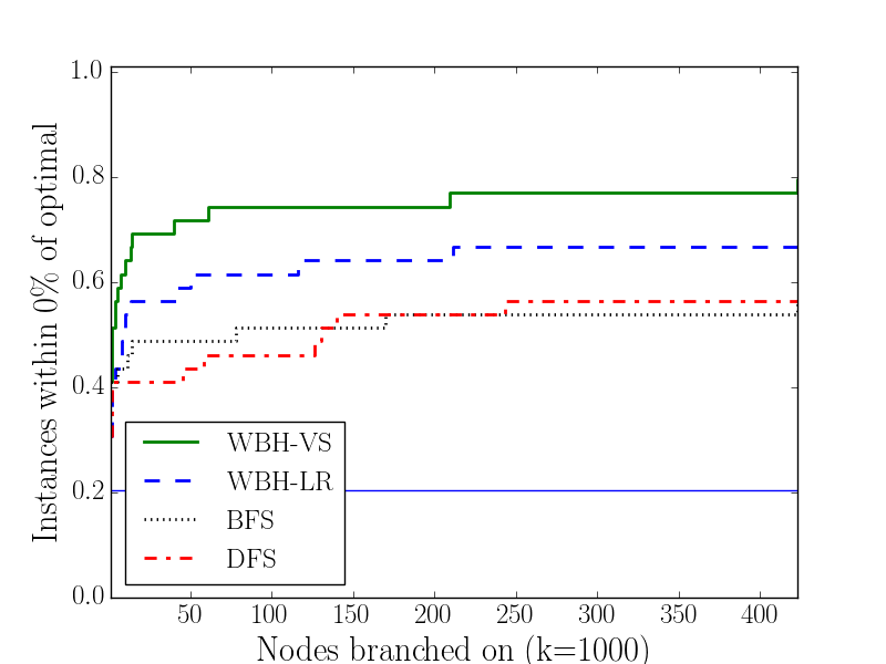
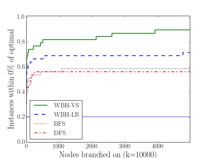
Figure 9: A performance profile showing the fraction of MM instances which a target bound is proved. The partial tree is limited to at most $1\,000$, or $10\,000$ internal nodes.

Figures 3, 5, 6,8 and 9 are a representative sample of performance profiles that indicate the fraction of instances (vertical axis) for which a given branching strategy proves a target bound after branching on a given number of nodes (horizontal axis). The target bound is typically within 0% or 5% of the optimal bandwidth (for the Random and MM instances), or $\phi$ (for the Turner instances). The branching strategies compared are WBH with greedy variable selection (WBH-VS) and WBH with layered branching order which alternates between placing vertices in the left and right of the permutation (WBH-LR), as well as DFS and BFS with the same alternating branching order. Where relevant the figures also show the fraction of instances for which the tighter of the graph theoretic lower bounds (5) and (6) achieved the target bound. The number of internal nodes are limited to $k\in\{100,1\,000,10\,000\}$; when the horizontal axis terminates before $k$ all of the curves are flat for a larger number of branches up to $k$. We omit results for the Turner instances with 1000 vertices, since the gap between the tightest graph theoretic lower bound and the upper bound $phi$ was found to be $0.35\%$ on average, leaving little room for improvement.

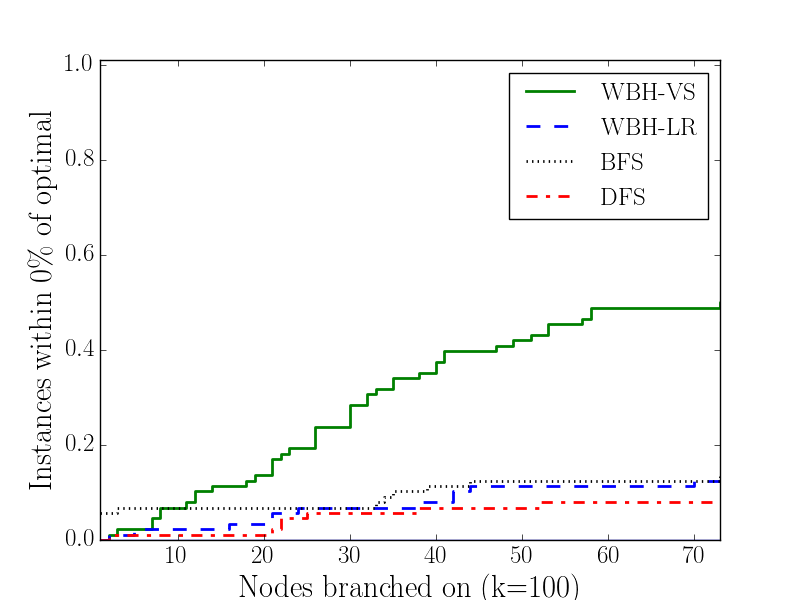
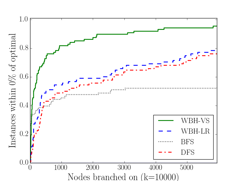
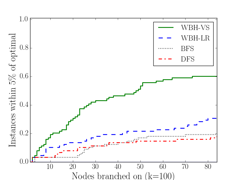
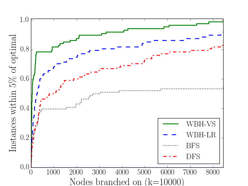
Figure 3: A performance profile showing the fraction of Random instances with 30 vertices for which a target bound is proved. The blue baseline is the fraction of instances where the unstrengthened graph theoretic bounds achieved the target bound. The partial tree is limited to $k=100$ or $k=10,000$ internal nodes.

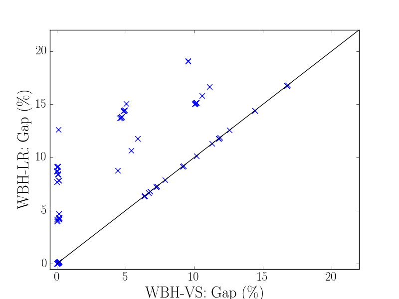
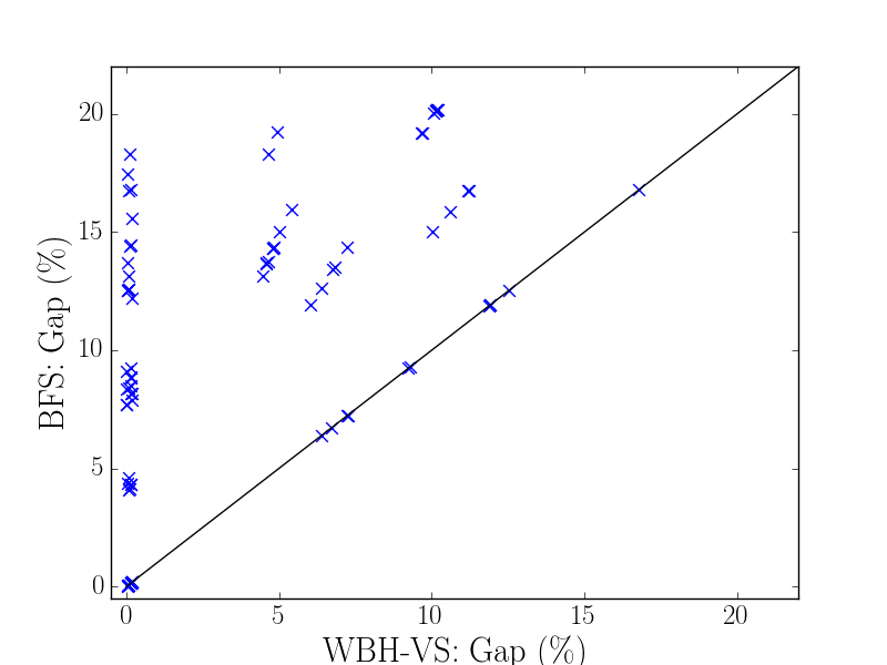
Figure 4: Scatter plot showing the relative performance of BFS and WBH-LR compared to WBH-VS on the 90 Random instances with 30 vertices after branching on 100 nodes.

The figures indicate that worst-bound branching with fixed variable order is superior to both breadth-first and depth-first branching, and far superior to the graph-theoretic bounds. Moreover, worst-bound branching with variable selection tightens the bound substantially, for any given time investment. In fact, on the Random, Turner30 and MM instances it obtains the optimal value for most instances after only modest computational effort. WBH-VS and WBH-LR retains a clear advantage over BFS and DFS on the larger MM instances. On the larger instances it is unsurprisingly more difficult for any of the branching methods to achieve the target bound in a limited number of nodes. On the Turner250 instances the worst-bound heuristic provides a smaller benefit over the alternatives, in part because the node limits are more restrictive in a large graph with an increased branching factor, and in part due of the fact that the gap between the graph theoretic lower bounds and $\phi$ is much smaller (see Table 2). Yet the worst-first heuristic continues to prove stronger bounds than BFS and DFS while requiring significantly less computation.

Figures 4, 7 and 10 are scatter plots comparing the gap between the lower and upper bound for the respective branching strategies on a per-instance basis after branching on a specified number of nodes. The plots for the omitted test sets are similar. We observe that WBH-VS inproves over WBH-LR and BFS on a significant fraction of the instances, including many which are solved optimally by WBH-VS while the alternative methods report gaps in excess of 5 or 10%.

Table 2 shows the average gap between the lower and upper bounds after branching on $100,1\,000$ or $10\,000$ nodes for each of the methods. As benchmark we also report the average gap between the strongest of the graph theoretic bounds and the best known upper bound. For all test sets, the gap is significantly reduced by WBH-LR and WBH-VS after branching on only 100 nodes. On all the test sets except Turner100, WBH-VS achieves an average gap of less than 1% after branching on $10\,000$ vertices. We also observe that the graph-theoretic bounds are far tighter on the Turner250 instances than any other, with an average gap of $4.7\%$. This decreases to $0.35\%$ in our randomly generated Turner1000 instances (not shown). Finally, we remark that it is perhaps somewhat surprising that DFS on occasion reports smaller gaps than BFS. This suggests that having strong upper bounds is useful even when solving the branching dual.

Table 2 reports the maximum frontier size encountered while branching on up to $k\in\{100,1\,000,10\,000\}$ nodes, averaged over the instances in each of the test sets. The maximum frontier size is the largest number of open nodes stored at any point during the computation. As expected, DFS leads to significantly smaller frontier sizes than any of the other methods since it quickly probes to a layer deep in the tree where the average branching factor is likely to be much lower than at the root node, and spends the bulk of the computation time at that depth. The memory requirements of WBH-VS is comparable to that of WBH-LR on the smaller instances, and within a factor of 2.5 on Turner250 and MM. Both variants of the worst-bound heuristic generally have much smaller frontier sizes than BFS.

Although our theoretical results do not guarantee the strongest bound for a given frontier size, we observe that the maximum frontier size is strongly correlated with the node limit $k$ and the size of the instance. A user who has limited memory available may select a node limit $k$ appropriately and strengthen the bound as much as possible subject to the node limit $k$ as guaranteed by Corollary 6.2. This is unlikely to differ much from the best possible bound subject to an explicit constraint on the frontier size.

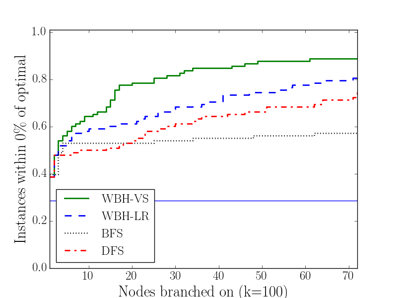
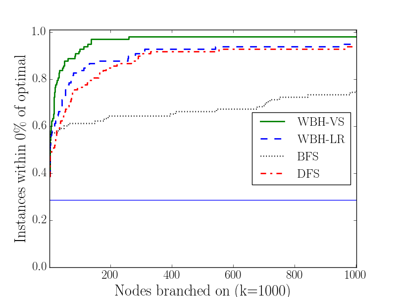
Figure 5: A performance profile showing the fraction of Turner instances with 30 vertices for which a target bound is proved. The partial tree is limited to at most $100$, or $1\,000$ internal nodes.

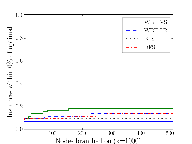
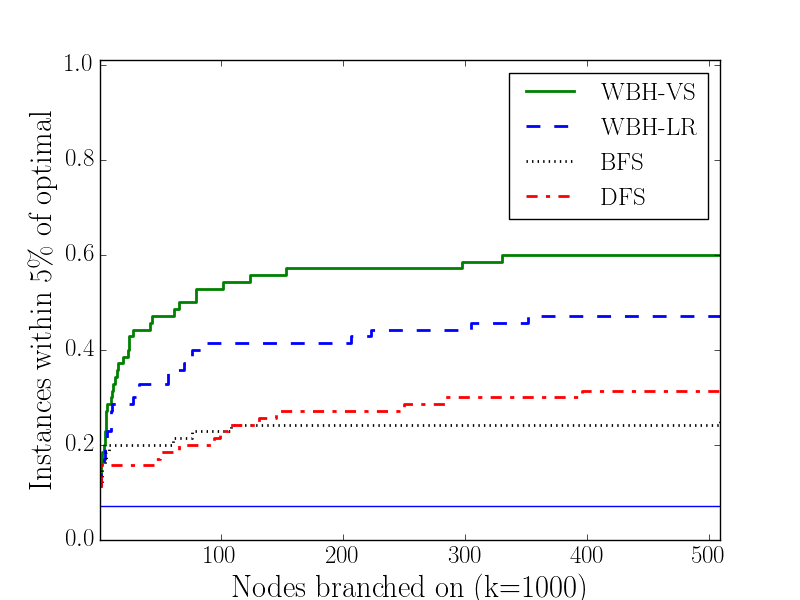
Figure 6: A performance profile showing the fraction of Turner instances with 100 vertices for which a target bound is proved. The partial tree is limited to at most $1\,000$ internal nodes.

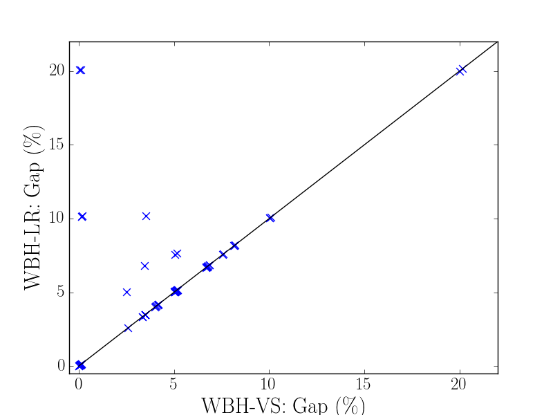
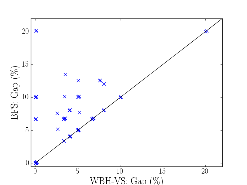
Figure 7: Scatter plot comparing WBH-VS with BFS and WBH-LR on the 70 Turner instances with 100 vertices after branching on $10\,000$ nodes.

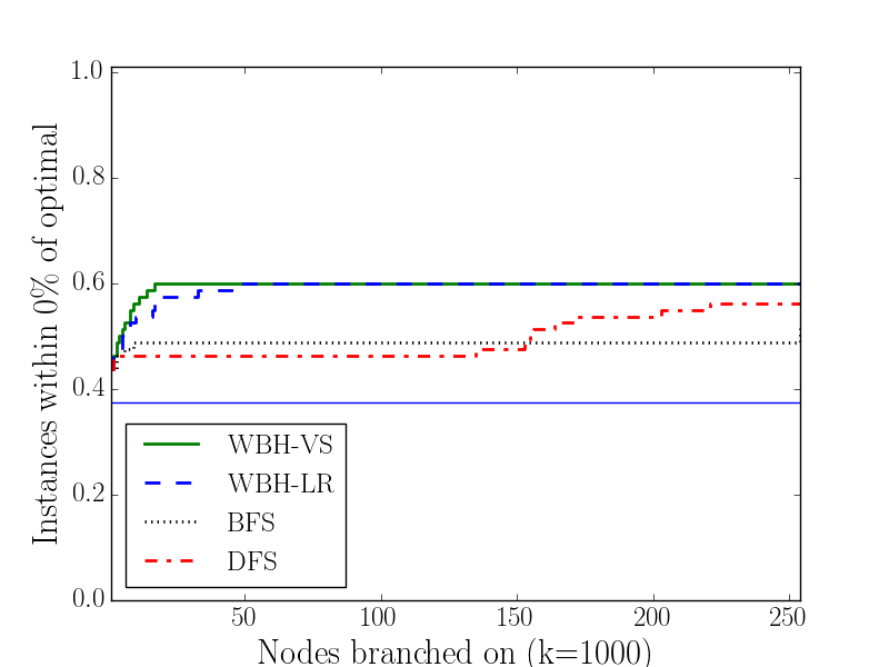
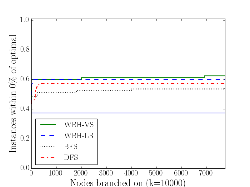
Figure 8: A performance profile showing the fraction of Turner instances with 250 vertices for which a target bound is proved. The partial tree is limited to at most $1\,000$, or $10\,000$ internal nodes.

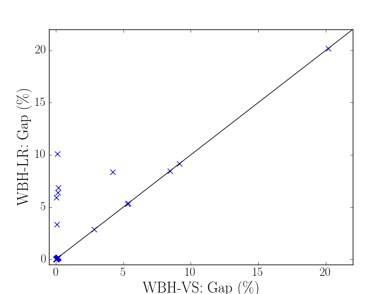
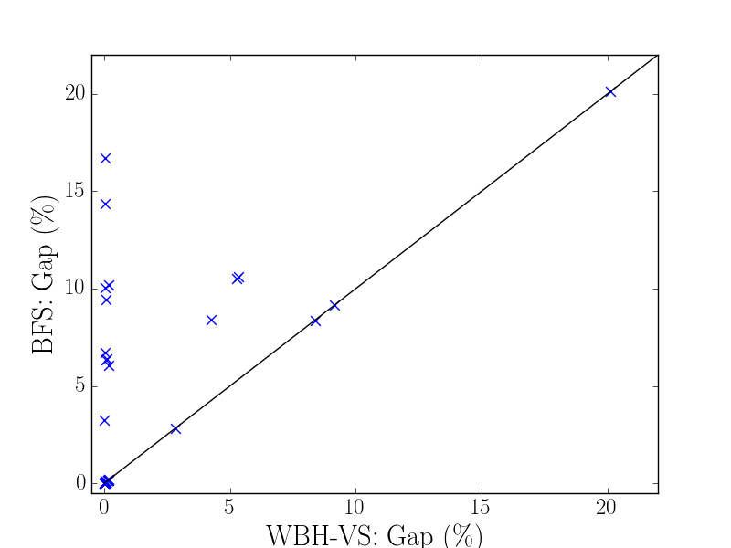
Figure 10: Scatter plot comparing WBH-VS with BFS and WBH-LR on the 39 MM instances after branching on $1\,000$ nodes.

Table 1: Average gap size (%) between the optimal lower bound and the best lower bound proved after branching on $100$, $1\,000$ and $10\,000$ nodes on the respective test instances. Benchmark (BM) is the strongest of the graph theoretic bounds.

	Turner30			Turner100			Turner250			Random30			Benchmarks
	Nodes branched on			Nodes branched on			Nodes branched on			Nodes branched on			Nodes branched on
Method	100	$1\,000$	$10\,000$	100	$1\,000$	$10\,000$	100	$1\,000$	$10\,000$	100	$1\,000$	$10\,000$	100	$1\,000$	$10\,000$
BFS	3.671	1.798	0.781	8.843	8.307	7.507	1.760	1.646	1.432	11.111	6.816	4.459	5.099	4.054	3.503
DFS	2.782	0.819	0.000	8.940	8.190	7.810	1.870	1.469	1.323	14.290	8.786	1.523	5.937	4.630	4.630
WBF-LR	1.497	0.564	0.000	6.871	6.100	5.707	1.214	1.068	1.016	8.098	3.350	0.723	3.368	2.334	2.067
WBF-VS	0.654	0.213	0.000	5.933	5.505	4.457	1.068	0.964	0.880	4.307	1.429	0.076	1.926	1.406	0.283
BM	27.99	27.99	27.99	18.07	18.07	18.07	4.729	4.729	4.729	32.53	32.53	32.53	20.54	20.54	20.54

Table 2: Average maximum frontier size after branching on $100$, $1\,000$ and $10\,000$ nodes on the test instances instances.

	Turner30			Turner100			Turner250			Random30			Benchmarks
	Nodes branched on			Nodes branched on			Nodes branched on			Nodes branched on			Nodes branched on
Method	100	$1\,000$	$10\,000$	100	$1\,000$	$10\,000$	100	$1\,000$	$10\,000$	100	$1\,000$	$10\,000$	100	$1\,000$	$10\,000$
BFS	557	$2\,541$	$7\,861$	$2\,371$	$22\,392$	$184\,578$	$4\,445$	$37\,049$	$310\,281$	975	$5\,800$	$24\,699$	$3\,794$	$28\,530$	$211\,566$
DFS	$82$	$82$	$82$	$753$	$753$	$753$	$2\,667$	$2\,880$	$2\,880$	$93$	$93$	$93$	$1\,640$	$1\,794$	$1\,794$
WBH-LR	227	984	$2\,968$	$1\,058$	$8\,461$	$73\,035$	$1\,306$	$10\,009$	$83\,734$	391	$2\,186$	$8\,395$	$1\,168$	$9\,667$	$78\,666$
WBH-VS	275	858	$2\,041$	$1\,926$	$15\,318$	$122\,814$	$2\,570$	$18\,238$	$140\,324$	573	$2\,107$	$6\,788$	$3\,321$	$19\,643$	$196\,432$

10 Conclusion

We studied the branching dual of an optimization problem for the purpose of strengthening an existing bound. We showed that for fixed variable selection, a natural worst-bound node selection heuristic is optimal for proving bounds with a given computational investment. We evaluated the worst-bound heuristic experimentally on the minimum bandwidth problem using a relaxation function in Caprara et al. (2011) and found that it is much more effective at proving bounds that depth-first or breadth-first search. Finally, we showed how combining this node selection heuristic with local search strategies for variable selection can lead to significant improvements in the quality of the bounds.

The branching dual method is proposed here primarily for combinatorial problems that have no useful integer programming model. In such cases, one need only determine how to strengthen a known bound, even a weak one, to reflect the fact that some variables have been fixed. However, the same technique can also be used to obtain bounds for integer or mixed integer programming models. In this case, modifying the linear programming bound to reflect fixed variables is trivial. The method can also applied at individual nodes of a conventional branch-and-cut tree to obtain bounds that may be tighter than those obtained from a linear relaxation with cutting planes. More generally, the method can be used for problems with a mixture of discrete variables (not necessarily integer) and continuous variables, so long as a relaxation value can be computed when some of the discrete variables have been fixed. These remain topics for future research.

References

- Achterberg (2007) Achterberg T (2007) Constraint Integer Programming. Ph.D. thesis, Technische Universität Berlin.
- Achterberg et al. (2005) Achterberg T, Koch T, Martin A (2005) Branching rules revisited. Operations Research Letters 33(1):42–54.
- Alvarez et al. (2017) Alvarez AM, Louveaux Q, Wehenkel L (2017) A machine learning-based approximation of strong branching. INFORMS Journal on Computing 29:185–195.
- Applegate et al. (2007) Applegate DL, Bixby RE, Chvátal V, Cook WJ (2007) The Traveling Salesman Problem: A Computational Study (Princeton University Press).
- Benichou et al. (1971) Benichou M, Gautier JM, Girodet P, Hentges G, Ribiere R, Vincent O (1971) Experiments in mixed-integer linear programming. Mathematical Programming 1:76–94.
- Bixby et al. (1995) Bixby RE, Cook W, Cox A, Lee EK (1995) Parallel mixed integer programming. Technical report CRPC-TR95554, Center for Research on Parallel Computation.
- Blum et al. (1998) Blum A, Konjevodand G, Ravi R, Vempala S (1998) Semi-definite relaxations for minimum bandwidth and other vertex-ordering problems. Proceedings of the thirtieth annual ACM symposium on Theory of computing, 100–105 (ACM).
- Caprara et al. (2011) Caprara A, Letchford AN, Salazar-González JJ (2011) Decorous lower bounds for minimum linear arrangement. INFORMS Journal on Computing 23:26–40.