Collective project

Abstract

The study of Frobenius endomorphism provides numerous information about its corresponding Abelian variety. To understand the action of the Frobenius endomorphism, one may be interested in its eigenvalues. According to Weil’s third conjecture ("Riemann hypothesis over finite fields"), they all have absolute value less than or equal to $2g\sqrt{p}$. Thus, the eigenvalues of the Frobenius endomorphism all belong to the same compact subset of the complex plane, and are roots of the same monic polynomial with integer coefficients (the characteristic polynomial of the Frobenius endomorphism). Such complex numbers are called algebraic integers "totally" in a compact subset, which means algebraic integers all conjugates of which belong to a same given compact subset of the complex plane.

The study of such algebraic integers helps to understand the eigenvalues of the Frobenius endomorphism, especially their distribution. In this paper, we will study the following question : under which conditions a compact subset of the complex plane has a finite or infinite number of algebraic integers totally in it ? The problem can be studied in light of the notion of capacity of a compact subset, which comes from potential theory. In this paper, we will present the theory of capacity and some theorems (Fekete, Szegö, Robinson) derived from it that partially answer the question: in the case of a union of real segments, when the capacity is smaller (resp. larger) than 1, it contains a finite (resp. infinite) number of algebraic integers totally in it. For instance, for real line segments, the limit length is 4.

This paper is written as part of a collective project conducted in École Polytechnique (France). It is aimed towards undergraduate audience in mathematics, with basic knowledge in algebra, topology, analysis, and dwells into a modern topic of research.

Preamble

0.1  Motivation

Since the XIX-th century, research in arithmetic uses concepts from other branches of mathematics, leading to great progress with surprising efficiency. One of the branches created by this diversification is arithmetic geometry, which combines algebra and geometry to solve number theory problems. A quick description of the success of this union can be found in [articlegéoarithmétique].

One of the main subject of study in this area is the behavior of geometric objects (e.g. "curves") defined over finite fields. These "curves" are rigorously defined as the domain on which a certain number of multi-variable polynomials defined over the considered finite field vanish. For instance, the first bisector is the domain in which the polynomial $P(X,Y)=X-Y$ vanishes. As a reminder, a finite field is a finite set with a well defined addition and multiplication. For example, we can take the field $\mathbb{F}_{p}=\mathbb{Z}/p\mathbb{Z}$, where $p$ is a prime number, as well as the extensions $\mathbb{F}_{p^{n}}$ obtained by adding the root of an irreducible polynomial of degree $n$.

One of the remarkable properties of these curves is that we can associate them with abelian groups in which it is possible – in a certain way – to "sum" two points on the curve, and to find an opposite to each point. These groups, called abelian varieties exhibit very interesting properties and are still today an active area of mathematical research, with numerous results [articleRechercheRécent][articleVariétés].

To study the curves over finite fields, a classical method is to study the action of homomorphisms (i.e. applications compatible with the algebraic structure of the field) on those curves. One of the most famous and important homomorphisms in such cases is the so-called Frobenius endomorphism $\mathrm{Fr}$ which raises the coordinates of a point of the curve to the $p$-th power, where $p$ is the characteristic of the field (the smallest integer such that $p\times 1=0$ in the field, with $1$ the unit of the field). In general algebra, the study of Frobenius endomorphism allows to deduce a number of properties on the set on which it acts. As such, it is natural to try to study it in the case of curves over finite fields. Especially, since $x^{p}=x$ for all $x\in\mathbb{F}_{p}$, the number of fixed points of the Frobenius endomorphism is the number of points of the curve with coordinates in $\mathbb{F}_{p}$. In the same way, the fixed points of $\mathrm{Fr}^{n}$ are the points of the curve whose coordinates belong to $\mathbb{F}_{p^{n}}$.

It is then possible to construct the generating function $\exp(\sum_{n\geq 1}N_{n}\frac{T^{n}}{n})$, where $N_{n}$ is the number of points of the curve with coordinates in $\mathbb{F}_{p^{n}}$. According to the Weil conjectures [articleFrob], this power series is actually a rational function : more precisely, a quotient $P(T)/(1-T)(1-pT)$ with $P\in\mathbb{Z}[X]$ a monic polynomial with integer coefficients. This polynomial is the characteristic polynomial of $\mathrm{Fr}$ acting – not on the curve as previously seen – but on the abelian variety defined from the curve. The eigenvalues of this Frobenius endomorphism are the root of the characteristic polynomial, which, according to Weil’s third conjecture, ("Riemann hypothesis over finite fields"), are all inferior in absolute value to $2g\sqrt{p}$, in which $g$ is the dimension of the abelian variety. In particular, they are all included in the same compact subset (i.e. closed and bounded) $K$ of the complex plane. The roots of such a polynomial are called algebraic integers totally included in $K$. Of course, all monic polynomials with such roots are not associated with Frobenius endomorphisms. But understanding the behavior of this kind of polynomials allows a better comprehension of Frobenius endomorphisms.

With that being said, it is natural to inquire about the distribution of those eigenvalues, which can be deduced from the distribution of algebraic integers totally in a compact subset. This distribution itself can be deduced from the case where $K$ is a real line segment, studied by Robinson who showed in 1962 the following result: if the length of $K$ is strictly more than 4, there is an infinite number of algebraic integers totally in it; if the length is strictly inferior to 4, there is only a finite number of such numbers. The case in which the length is exactly 4 is – for now – only solved for a few special cases. The paper we present here gives a proof of this result.

0.2  Outline of the paper

In a formal way, algebraic integers are complex numbers which are the roots of a monic polynomial with coefficients in $\mathbb{Z}$. We shall call $\mathbb{Q}$-conjugates of an algebraic integer $\alpha$ the roots of the unique monic polynomial $P$ with rational coefficients of minimal degree for which $P(\alpha)=0$ (minimal polynomial). Given a compact set $K$ of $\mathbb{C}$, we say that an algebraic integer is totally in $K$ if all his $\mathbb{Q}$-conjugates are in $K$. We call degree of an algebraic integer the degree of his minimal polynomial.

The study of the distribution of algebraic integers totally in a real line began in the beginning of the XX-th century, with a first result from Schur in 1918 which solves the case of real lines with length strictly below 4. Many other results follow in the next years. Then, some 40 years later, Robinson eventually demonstrates his theorem, leaving only the case of length 4 unresolved.

The proof we shall give here for Robinson’s theorem follows an article from Jean-Pierre Serre [serre2018bourbaki] which summarizes a lecture given during the Bourbaki seminar of March 2018 in Paris. The purpose of the present paper is to be understandable by a non-specialist audience, but one that has a solid grasp on the basic elements of algebra (group, polynomials), topology (weak convergence) and analysis (continuity, basic complex analysis). It seems to us that an undergraduate audience can follow our work and the proof we shall give without too much trouble. The more interested readers can find in the appendix additions on measure theory, on more subtle analysis points used in our reasoning, as well as proofs deemed too technical and without much interest as far as understanding the essence of this proof goes.

In the first part (Elementary remarks), we shall make a range of first observations on this problem, which will lead to ideas of proof, or invalidate certain proof schemes that could be thought of. This part includes an algorithmic approach that allows us to get an intuition on the result (although the programs’ complexity does not allow for a very deep dive into polynomials of high degrees). Finally, we will demonstrate a first result first found by Kronecker (1857) which deals with the case where the compact subset of the complex plane is the unit circle. From this case, we will deduce the behavior of the real line $[-2,2]$, and, more widely, of any real line of the form $[n-2,n+2]$, with $n\in\mathbb{Z}$. From these remarks, we will give first bounds for the length of real lines containing an infinite/finite number of algebraic integers totally in it.

In the second part, we will look into the theory of capacity, which is the natural frame of study for dealing with the " size" of a compact set for this problem. This notion of capacity is deeply linked to the concepts introduced in measure theory, and some of the results from this part – once combined with results from the last part – allow us to prove a slightly stronger result than Robinson’s theorem. In particular, we prove the convergence (in a certain sense) of a measure associated with a sub-sequence of polynomials towards the measure of equilibrium of the compact set.

We will then show in the third part Fekete’s theorem LABEL:thmFekete which solves the case of a real line of length strictly less than four, then, Fekete-Szegö’s theorem LABEL:thmFeketeSzego which is the equivalent of Robinson’s theorem for complex compact subset of the complex plane (as opposed to the real lines of Robinson’s theorem). We will see how the proof of this theorem is not sufficient to yield the real case, although some ideas can be reused to solve the latter, which is why the study of this theorem is very interesting for this proof.

In the last part of this paper, we will eventually give the full proof of Robinson’s theorem, using the tools developed in the first parts as well as a few results pertaining to the field of algebraic geometry. After a quick introduction to the core concept of algebraic curves, we will use those results to finish the proof of the main result of this paper.

1Elementary remarks

Let us start by reminding ourselves of the definition of our object of study: algebraic integers totally in a compact set.

Definition 1.1 

1. An algebraic integer is a complex number that is a root of some monic polynomial with coefficients in $\mathbb{Z}$.

2. Given an algebraic integer $\zeta\in\mathbb{C}$, we call minimal polynomial of $\zeta$ the unique monic polynomial with integer coefficients among these with $\zeta$ as a root.

3. Let us denote by $\mathrm{Gal}(\zeta)$ the set of all roots of the minimal polynomial of $\zeta$.

4. Let $E$ be a subset of $\mathbb{C}$ and $\zeta$ an algebraic integer. We say that $\zeta\in\mathbb{C}$ is totally in $E$ if $\mathrm{Gal}(\zeta)\subset E$.

1.1  First results

In this first section, we will start by stating three "elementary" remarks about the problem: first, at a fixed degree, there is only a finite number of algebraic integers totally in a given compact set; then, the derivatives of a minimal polynomial of algebraic integers totally in a compact set have interesting properties; finally, if $K_{1}\subset K_{2}$ are two compact sets, then the numbers of algebraic integers totally in $K_{1}$ and $K_{2}$ respectively, can be compared.

Remark 1.1 

Let $K$ be a compact subset of $\mathbb{C}$. Let $P$ be a monic polynomial of degree $n$ the roots of which are all in $K$, we can upper bound the $k$-th coefficient of $P$ by $\sup(K)^{k}\binom{n}{k}$. It is enough to assure that, at fixed degree, there exists a finite number of such polynomials with all roots in $K$, and therefore a finite number of algebraic integers of degree $n$ totally in $K$.

This remark leads us to several interesting approaches:

• We can find (algorithmically) the adequate polynomials of small degrees.

• If we want to prove that there exists a finite number of algebraic integers in a compact set, it is enough to prove that the degree of such an integer is bounded.

Remark 1.2 

Let us consider a monic polynomial $P$ with integer coefficients whose roots are algebraic integers totally in a compact set $K$, where the degree of $P$ is greater than or equal to $2$, its derivative is not a monic polynomial. However it is still a polynomial with integer coefficients, and its roots are still in $K$, if this compact set is convex (which is the case for real line segments). Indeed, it follows from Gauss-Lucas theorem that the roots of $P^{\prime}$ are in the convex hull of the set of roots of $P$.

Therefore we notice that the knowledge of $P^{\prime}$ gives us information on the roots of $P$. This idea will be useful when we compute algorithmically algebraic integers totally in a compact set.

Remark 1.3 

Let $K_{1}$ and $K_{2}$ be $2$ compact sets such that $K_{1}\subset K_{2}$, then there is at least as many algebraic integers totally in $K_{2}$ as those totally in $K_{1}$ (since any algebraic integer totally in $K_{1}$ is an algebraic integer totally in $K_{2}$). This somewhat obvious remark will be of great use for proofs where it is easier to work on a smaller compact set.

1.2  Algorithmic approach

In order to get an intuition about the algebraic integers totally in a compact set, we have decided to conceive and implement an algorithm listing algebraic integers totally in a line segment, the minimal polynomial of which, is of fixed degree. These results will later be compared to the demonstrated theorems.

Let $K$ be a compact subset of $\mathbb{C}$. Two questions were kept to be answered by numerical experiments:

• What are the algebraic integers totally in $K$? A particular focus is done on the distribution of such numbers. The results can be compared to the cases studied in section 1.3. This question seems difficult because it requires a fine knowledge of the algebraic integers totally in $K$. That is why the core question of our paper is actually :

• Is there an infinite number of algebraic integers totally in $K$ ? The numerical answer to this question can be compared to the results of sections LABEL:sectionthFEk and LABEL:section3.

First, we will state the algorithmic principle that we use, then we will comment on the results we obtained.

1.2.1  The algorithmic principle

In order to get numerical results, only monic polynomials with integer coefficients, the degree of which, is less than a given integer $n$ will be studied. The goal is to find a list as short as possible with all minimal polynomials, with degree less than $n$, of algebraic integers totally in $K$.

The remark 1.1 allows to give bounds to the coefficients of polynomial with a given degree, the roots of which, are all in $K$. Therefore, for a given degree, the polynomials that could be the minimal polynomial of an algebraic integer totally in $K$ can be enumerated:

Algorithm 1 Naive algorithm

  $l$ empty list

  for all $P$ monic polynomial of degree less than n, the coefficients of which, are integers in the bounds of remarks 1.1 do

     if the roots of $P$ are totally in $K$ then

        add the roots of $P$ to $l$

     end if

  end for

  return  $l$

However, this method is not very efficient. Indeed, the complexity is greater than the product of the double of the bounds:

$$\prod_{k=1}^{n}(2\sup(K))^{k}\binom{n}{k}C(n)\geqslant(2\sup(K))^{n^{2}/2},$$

where $C(n)$ is the complexity of computing the roots of a polynomial of degree $n$ (done by computing the eigenvalues of the companion matrix). For instance, when the compact set $K$ is a line segment subset of [-2.5,2.5], this algorithm cannot list the algebraic integers totally in $K$ with minimal polynomial of degree higher than $n=4$. This data is unfortunately not enough to make interesting conjectures.

Since we mainly focus on the case of real segments, we implemented another specific algorithm for segments of $\mathbb{R}$. Remark 1.2 can therefore apply and gives a great improvement in efficiency. Indeed, when $K$ is a segment of $\mathbb{R}$, for all algebraic integers totally in $K$, all the derivatives of its minimal polynomial have simple roots and all the zeros are in $K$. More generally, let $l<n-1$ and let us consider the polynomials $P=\displaystyle\sum^{n}_{k=0}a_{k}X^{k}$ where the $n-l-1$ greatest coefficients $a_{l+1},\dots,a_{n-1}$ are fixed and $a_{n}=1$. Then $P^{(l)}=l!a_{l}+\displaystyle\sum_{k=1}^{n-l}\frac{(l+k)!}{k!}a_{l+k}X^{k}$ has $n-l$ roots in $K$. More specifically, $-a_{l}$ is between the maximum of all local minimums and the minimum of all local maximums of $\displaystyle\sum_{k=1}^{n-l}\frac{(l+k)!}{k!}a_{l+k}X^{k}$. Thus, by repeating for $l$ ranging from $n-2$ to $0$, we obtain stricter constraints on $a_{0},\dots,a_{n-1}$ and thus a list of polynomials likely to have all their roots in $K$ much more restricted than in the naive algorithm. In summary, the limits of the remark 1.1 have been refined by taking into account the value of the other coefficients already set. Thus the polynomials whose roots are calculated are much less numerous and of lower degree, which explains why this algorithm is more efficient than the previous one. Thanks to this optimization, it was possible to obtain all algebraic integers, whose minimum polynomial’s degree is at most $n=7$ for segments included in $[-2.5,2.5]$. The analysis of figure 2 corroborates this observation. While it has been calculated that the naive algorithm has a complexity of at least $C^{n^{2}}$, the second algorithm has an experimental complexity close to $15^{n}$.

After writing this algorithm, we tried to compare it with the state of the art. In [articleAlgo], the authors combine techniques very close to ours but more refined with algebraic properties to solve a problem close to ours. Their algorithm allows to go up to degree 13 in a reasonable time. But unfortunately, we cannot directly apply their algorithm to our problem.

1.2.2  Results

Considering remark 1.3, an algebraic integer totally in a compact set $K$ is totally in all compact sets containing $K$. We can think that "large" compact sets will have an infinite number of algebraic integers while "small" compact sets will have a finite number.

To verify this, we have plotted the evolution of the number of algebraic integers totally in $K$ according to the degree of their minimal polynomial for different segments $K$ of $\mathbb{R}$. The results in figure 3 show that the length 4 is the boundary between "small" and "large" segments. For segments with lengths less than 4, there are fewer and fewer new algebraic integers as the degree increases (blue, orange). On the contrary, for segments longer than 4, there are more and more (green, red, purple). This observation remains valid when translating the segments.

These observations are in accordance with the theorems that we will demonstrate in this paper. The behavior of "small" segments is treated by Fekete’s theorem LABEL:thmFekete and that of "large" segments by Robinson’s theorem LABEL:thmRobinson.

When $K=[-2.2]$, we can notice that the number of new algebraic integers totally in $K$ found at the $n$ degree seems to increase, but not exponentially (figure 2). We can verify that the algebraic integers found are of the form $2\cos(\frac{2k\pi}{m})$ with $k$ and $m$ integers. We will see in the following subsection (1.1) that the algebraic integers totally in $[-2.2]$ are the $2\cos(\frac{2k\pi}{m})$ with $k$ and $m$ integers. However, the algorithm does not find them by increasing $m$.

Beyond the finiteness of the set of algebraic integers totally in a compact set, one can be interested in the distribution of these numbers. The figure 4 shows that the distribution is essentially the same both when translating slightly and when the length changes. Moreover, this distribution is similar to that of the roots of the Chebyshev polynomials.

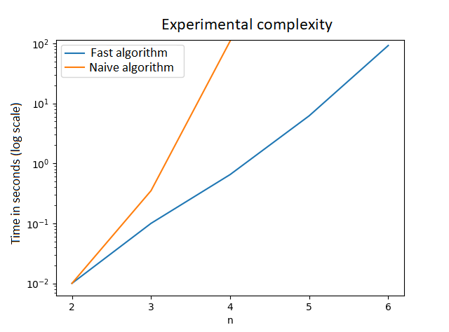
Figure 1: Experimental complexity of the two algorithms (length = 3.9)

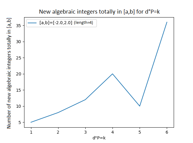
Figure 2: Number of new algebraic integers in function of the degree of the minimum polynomials for $K=[-2,2]$

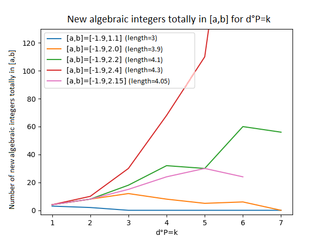
Figure 3: Number of new algebraic integers found in function of the degree of the polynomials traversed

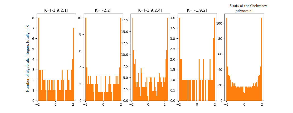
Figure 4: Distribution of algebraic integers of lower degree for different segments compared to that of the roots of Chebyshev polynomials

1.3  Two elementary cases : $\mathbb{U}$ and $[-2,2]$

Let us start with the well known cases of the unit circle and segments with length $4$ and integer end points.

1.3.1  $K=\mathbb{U}$ : Kronecker’s theorem

When $K=\mathbb{U}$ is the unit circle, Kronecker’s theorem gives us the following result :

Theorem 1.1  (Kronecker). 

Let $P\in\mathbb{Z}[X]$ be a monic polynomial whose complex roots are all in the unit circle $\mathbb{U}$, then its roots are roots of unity.

Let us start with the following lemma :

Lemma 1.1 

Let $n,k\in\mathbb{N}$ and $Q$ be a polynomial with expression $\displaystyle\prod_{i=1}^{n}(X-\alpha_{i})$.
If $Q\in\mathbb{Z}[X]$, then $Q_{k}(X):=\displaystyle\prod_{i=1}^{n}(X-\alpha_{i}^{k})\in\mathbb{Z}[X]$.

Proof.

Let us consider such a polynomial $Q$ and integers $n$ and $k$. The Frobenius companion matrix $M$ of $Q$ is a matrix of $M_{n}(\mathbb{Z})$ whose characteristic polynomial is $Q$. Therefore the $\alpha_{i}$ are the eigenvalues of $M$. $M$ is similar to an upper triangular matrix with main diagonal $\alpha_{1},\dots,\alpha_{n}$, which results in $M^{k}$ being similar to an upper triangular matrix with main diagonal $\alpha_{1}^{k},\dots,\alpha_{n}^{k}$. Thus, the $\alpha_{i}^{k}$ are the eigenvalues of $M^{k}$ with the same multiplicity as for $M$. It implies that $Q_{k}$ is the characteristic polynomial of $M^{k}$. Since this matrix has integer coefficients, $Q_{k}$ has as well. ∎

Let us prove Kronecker’s theorem:

Proof. Let us consider $P=X^{n}+p_{n-1}X^{n-1}+\dots+p_{0}\in\mathbb{Z}[X]$ a monic polynomial such that $Z(P)\subset\mathbb{U}$, where $Z(P)=\{\alpha_{1},\dots,\alpha_{n}\}$ is the set of the complex roots of $P$. It follows from the Vieta’s formulas that:

$$p_{n-k}=(-1)^{k}\displaystyle\sum_{J\in\mathcal{P}_{k}([1,\dots,n])}\displaystyle\prod_{i=1}^{k}\alpha_{j_{i}}.$$

Since the $\alpha_{i}$ are of magnitude $1$, the triangle inequality gives us that $|p_{n-k}|\leq\binom{n}{k}$. The coefficients of $P$ being integers, we deduce that $\mathcal{E}_{n}$, the set of polynomials of degree $n$ which verify the hypotheses of the theorem, is a finite set. It implies that $\mathcal{R}_{n}$, the set of roots of polynomials in $\mathcal{E}_{n}$ is also finite.

Let $\alpha_{i}$ be a root of $P$ and let us consider the multiplicative group generated by $\alpha_{i}$, $G=\{\alpha_{i}^{k},k\in\mathbb{Z}\}$. With the notations from lemma  1.1, for all $k\in\mathbb{Z}$, $\alpha_{i}^{k}$ is a root of $Q_{k}\in\mathcal{E}_{n}$ according to the lemma. Therefore, $G$ is a finite group since $G\subset\mathcal{R}_{n}$. As a result, there exists integers $k<k^{\prime}$ such that $\alpha^{k}=\alpha^{k^{\prime}}$, which means $\alpha^{k^{\prime}-k}=1$. ∎

Remark 1.4 

Let us give another proof of lemma 1.1 using symmetric polynomials. Let us consider $P=\displaystyle\sum_{j=1}^{n}p_{j}X^{j}=\displaystyle\prod_{i=1}^{n}(X-\alpha_{i})\in\mathbb{Z}[X]$ and $Q=\displaystyle\sum_{j=1}^{n}q_{j}X^{j}=\displaystyle\prod_{i=1}^{n}(X-\alpha_{i}^{k})$. Let $S_{j}$ denote the $j$-th elementary symmetric polynomial in $n$ variables. It follows from the Vieta’s formulas that : $p_{n-j}=(-1)^{j}S_{j}(\alpha_{1},\dots,\alpha_{n})$ and $q_{n-j}=(-1)^{j}S_{j}(\alpha_{1}^{k},\dots,\alpha_{n}^{k})$. According to the fundamental theorem of symmetric polynomials,

there exists a polynomial $R\in\mathbb{Z}[X_{1},\dots,X_{n}]$ such that

$$S_{j}(X_{1}^{k},\dots,X_{n}^{k})=R(S_{1},\dots,S_{n})$$

Therefore, the coefficients of $Q$

$$q_{n-j}=(-1)^{j}S_{k}(\alpha_{1}^{k},\dots,\alpha_{n}^{k})=(-1)^{j}R(-p_{n-1},\cdots,(-1)^{n}p_{0})$$

are integers.

Actually, the fundamental theorem of symmetric polynomials applies to all the symmetric polynomials, so that all the symmetric combinations of $\alpha_{1},\dots,\alpha_{n}$, with integer coefficients, are integers.

Remark 1.5 

Note that the use of companion matrices in the proof of lemma 1.1 allows us to give a direct proof of this following particular case of the fundamental theorem of symmetric polynomials: "there exists $R\in\mathbb{Z}[X_{1},\dots,X_{n}],$ such that $S_{j}(X_{1}^{k},\dots,X_{n}^{k})=R(S_{1},\dots,S_{n})$".

Indeed, using the previous notations, let $M$ be the companion matix of $P$.

$$\forall\,1\leqslant i,j\leqslant n,\quad M_{i,j}\in\{S_{j}(\alpha_{1},\dots,\alpha_{n}))\,|\,0\leqslant j\leqslant n\}\cup\{0,1\}.$$

We deduce from it that :

$$\forall\,(i,j),\quad M_{i,j}\in\mathbb{Z}[S_{0}(\alpha_{1},\dots,\alpha_{n}),\dots,S_{n}(\alpha_{1},\dots,\alpha_{n})].$$

Thus the coefficients of the characteristic polynomial of $M^{k}$ are in $\mathbb{Z}[S_{0}(\alpha_{1},\dots,\alpha_{n}),\dots,S_{n}(\alpha_{1},\dots,\alpha_{n})]$. However, these coefficients turn out to be, regardless of the sign, the $(S_{i}(\alpha_{1}^{k},\dots,\alpha_{n}^{k}))_{0\leqslant i\leqslant n}$.
We conclude that :

$$\forall\,0\leqslant i\leqslant n,\quad S_{i}(\alpha_{1}^{k},\dots,\alpha_{n}^{k})\in\mathbb{Z}[S_{0}(\alpha_{1},\dots,\alpha_{n}),\dots,S_{n}(\alpha_{1},\dots,\alpha_{n})].$$

Conclusion of the case $K=\mathbb{U}$ :

algebraic integers totally in $\mathbb{U}$ are the roots of unity, and there is an infinite number of them. We have an example of a compact set with an infinite number of algebraic integers totally in it.

1.3.2  $K=[-2,2]$

Proposition 1.1 

Let us consider $P\in\mathbb{Z}[X]$ a monic polynomial such that $Z(P)\subset[-2;2]$.
The roots of $P$ all have the following expression: $z+\overline{z}$, where $z$ is a root of unity.

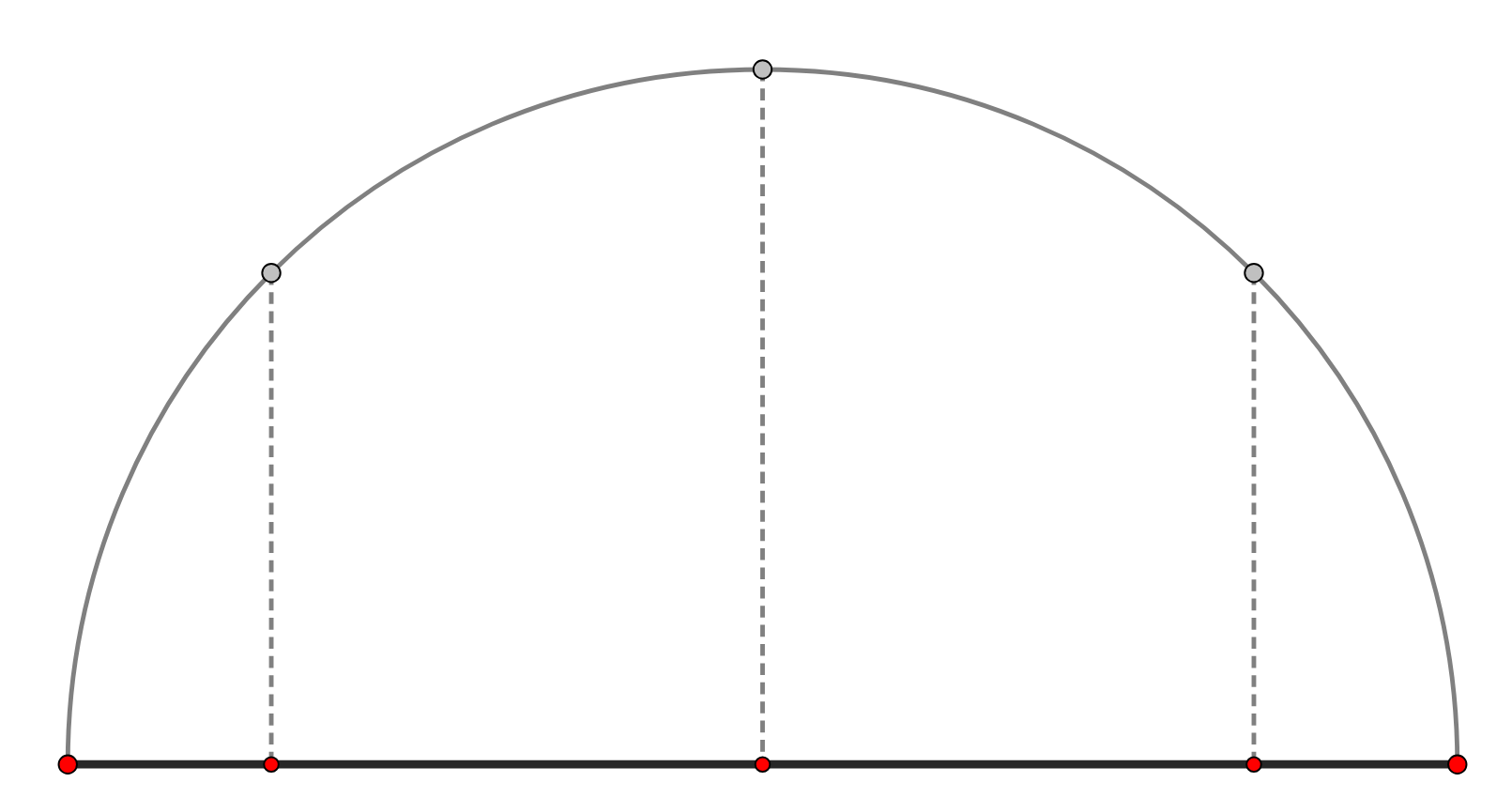
Figure 5: examples of points totally in $K=[-2,2]$

Proof. Let $P$ be a polynomial of degree $n$ verifying the assumptions of the proposition. Let us consider $Q=X^{n}P(X+\frac{1}{X})$. Using the binomial formula, we show that $Q$ is a monic polynomial of degree $2n$ with integer coefficients. Let us note that $0$ is not a root of $Q$ since the polynomial’s constant coefficient equals $1$. Therefore, for all $z\in\mathbb{C}$,

$$Q(z)=0\Leftrightarrow P(z+\frac{1}{z})=0.$$

Let $z$ be a complex root of $Q$. Then, $z+\frac{1}{z}$ is a root of $P$, and $z+\frac{1}{z}\in[-2,2]$. In particular, $z+\frac{1}{z}$ is a real number. If we write the obvious equality between this real number and its complex conjugate, we get that $\rho\sin(\theta)=\frac{1}{\rho}\sin(\theta)$, where $\rho$ and $\theta$ are the modulus and an argument of $z$ respectively. Two cases are possible:

• if $\sin(\theta)=0$, then $z\in\mathbb{R}$. In order to verify $z+\frac{1}{z}\in[-2,2]$, studying the sign of this expression shows us that $z=\pm 1$.

• if $\rho=\frac{1}{\rho}$, $\rho=1$, since the modulus is a non-negative number.

In all cases, $z\in\mathbb{U}$. It follows from Kronecker’s theorem that all the roots of $Q$ are roots of unity.

Let $r$ be a root of $P$. Since $r\in[-2,2]$, we can write $r=z+\overline{z}$, with $z=\frac{r}{2}+i\sqrt{1-\frac{r^{2}}{4}}$. Since $z\in\mathbb{U}$, $r=z+\frac{1}{z}$. Therefore, $z$ is a root of $Q$, which means that $z$ is a root of unity. ∎

Corollary 1.1 

The algebraic integers totally in $[-2,2]$ are real numbers with the following expression: $z+\overline{z}$, where $z$ is a root of unity.

Proof. The previous proposition shows us that the algebraic integers totally in $[-2,2]$ all have the following expression: $z+\overline{z}$, where $z$ is a root of unity. Let us prove the reciprocal implication.

Let $(U_{n})_{n}$ be the Chebyshev polynomials of the second kind defined as follows:

$$U_{0}=1\text{ et }\displaystyle U_{n+1}=2XU_{n}-U_{n-1},\ \ \forall n\geq 1.$$

We use induction on $n$ to show that $P_{n}(X)=U_{n}(\frac{X}{2})$ are monic polynomials of degree $n$ and with integer coefficients. They verify that $\forall\theta\in\mathbb{R}\setminus\pi\mathbb{Z}\quad\frac{\sin\left((n+1)\theta\right)}{\sin\theta}=P_{n}(2\cos\theta)$. We deduce from it that:

$$\forall n\geqslant 1,Z(P_{n})=\{2\cos{\frac{k\pi}{n+1}},\quad\forall k\in\{1,\ldots,n\}\}\subset[-2,2].$$

Therefore, for all $n\geqslant 1,Z(P_{n})$ is a set of algebraic integers totally in $[-2,2]$, which implies that for any root of unity $z$, $z+\overline{z}$ is totally in $[-2,2]$. ∎

Conclusion of the case $K=[-2,2]$ :

algebraic integers totally in $[-2,2]$ are the $z+\frac{1}{z}$, with $z$ some root of unity.

It follows from translating the previous result, this claim for any segment of $\mathbb{R}$ with length $4$ and integer end points:

Corollary 1.2 

Let $K=[n-2,n+2]$ be a real segment with length $4$, integer endpoints and $n\in\mathbb{Z}$ its middle point. The algebraic integers totally in $K$ are $n+z+\frac{1}{z}$, with $z$ a root of unity.

Proof. Let $P\in\mathbb{Z}[X]$ be a monic polynomial such that $Z(P)\subset[n-2,n+2]$ and let us consider $Q=P(X+n)$. Since $n\in\mathbb{Z}$, $Q$ is a monic polynomial with integer coefficients, and $Z(Q)\subset[-2,2]$. The proposition 1.1 allows us to conclude. ∎

From this particular case, we deduce a more general theorem which gives us a first piece of information:

Theorem 1.2  (Upper bound of the minimal length to contain an infinite number of algebraic integers totally in a segment). 

Segments with length greater than or equal to 5 have an infinite number of algebraic integers totally in them.

Proof. Segments with length $5$ contain a segment with length $4$ and integer endpoints, and according to remark 1.3, they contain at least as many algebraic integers as the smaller segments, therefore containing an infinite number, according to corollary 1.2. ∎

A first stage of the work was done with general remarks, an algorithmic approach to convince ourselves of the result and a first particular case. Let us now build a general framework to tackle the general case of the theorem.

2Capacity theory

First and foremost, let us focus our interest on the notion of capacity. It is a non-negative number describing the size of a set, but not a geometric size related to its measure : the terminology comes from physics, more specifically, from the capacity of a capacitor, which describes the ability of a set to contain electric charges. We shall see that it is an "adequate " definition of the size of a compact set when it comes to algebraic integers. This notion gives us a criterion which allows us to determine whether or not a compact set has an infinite number of algebraic integers totally in it (cf. LABEL:section3), with Fekete’s and Fekete-Szegö’s theorems.

The goal of this section is to give three equivalent definitions of the notion of capacity : transfinite diameter (2.1), logarithmic capacity (2.2) and the Chebyshev’s constant (2.4). The main theorem of this section is theorem LABEL:chebEgalCapaEgalTau which proves the equivalence between the three definitions, and states important properties of objects which allow us to link these three approaches: Fekete’s measures, equilibrium measure, equilibrium potential, Fekete’s polynomials, Chebyshev polynomials… In section 2.3, we will also prove a formula to calculate a type of capacity thanks to semi harmonic functions: this section, which is quite technical, can be skipped at first reading.

We will first introduce the notion of transfinite diameter of a compact set thanks to Fekete points ; then we will study the notion of logarithmic capacity and equilibrium measure before unifying these two notions. Finally we will give a third definition of the capacity using Chebyshev polynomials. Thanks to this last approach we will be able to calculate the capacity of segments.

2.1  Transfinite diameter, Fekete points

To get a first intuition, let us consider a geometric problem from electrostatics: let us place electrons in a bounded domain. These electrons will tend to maximize their mutual distances in order to minimize the overall energy. In $3$ dimensions, the force is proportional to the square of the inverse of the distance, and the potential is proportional to the inverse of the distance. Since we are working in the two-dimensional complex plane, the force is proportional to the inverse of the distance and the potential is proportional to $\log$ of the distance.

Given $K$ a compact subset of $\mathbb{C}$ and $z_{1},\dots,z_{n}\in K$, let us define the potential at point $z_{i}$ (which can be equal to $+\infty$) as follows :

$$U_{z_{1},\dots,z_{n}}(z_{i})=-\sum_{j\neq i}\log\left\lvert z_{j}-z_{i}\right\rvert.$$

Let us also define the energy of the configuration $(z_{1},\dots,z_{n})$ as the mean of the potentials at each point :

$$E(z_{1},\dots,z_{n})=-\frac{2}{n(n-1)}\sum_{i<j}\log\left\lvert z_{i}-z_{j}\right\rvert=-\log\prod_{i<j}\left\lvert z_{i}-z_{j}\right\rvert^{\frac{2}{n(n-1)}}$$

Let us focus on minimizing the energy of the compact set $K$ for a given number $n$ of points :

$$E(K)=\min_{z_{1},\dots,z_{n}\in K}E(z_{1},\dots,z_{n})=-\log\max_{z_{1},\dots,z_{n}\in K}\prod_{i<j}\left\lvert z_{i}-z_{j}\right\rvert^{\frac{2}{n(n-1)}}$$

The lower bound is reached since $K$ is compact, hence the $\min$ in the optimization formula. The points where this minimum is reached are called the Fekete points :

Definition 2.1  (Fekete points). 

Let $K$ be a compact subset of $\mathbb{C}$. Let us define

$$\delta_{n}(K)=\max_{z_{1},\dots,z_{n}\in K}\prod_{i<j}\left\lvert z_{i}-z_{j}\right\rvert^{2/n(n-1)}$$

This maximum value is reached at the Fekete points (of degree $n$).

Remark 2.1 

It matches the definition of the usual diameter for $n=2$.

Lemma 2.1 

let $f:K\times K\to\mathbb{R}\cup\{-\infty\}$ be a function and for all $n\in\mathbb{N}^{*}$, let us consider

$$m_{n}^{f}(K)=\sup_{x_{1},\dots,x_{n}\in K}\frac{1}{n(n-1)}\sum_{i\neq j}f(x_{i},x_{j}).$$

The sequence $(m_{n}^{f}(K))_{n}$ is decreasing.

Proof. Let $n\geq 1$, and $x_{1},\dots,x_{n+1}\in K$ (not necessarily distinct). We obtain the following equality:

$$\frac{1}{n(n+1)}\sum_{i\neq j}f(x_{i},x_{j})=\frac{1}{n+1}\sum_{k=1}^{n+1}\left(\frac{1}{n(n-1)}\sum_{i\neq j,i\neq k,j\neq k}f(x_{i},x_{j})\right);$$

indeed, it is easily verified by calculating the coefficients of $f(x_{i},x_{j})$ on each side: the term $f(x_{i},x_{j})$ on the right is only affected by the $k\in[\![1,n+1]\!]\backslash\{i,j\}$ so there are $n-1$ choices. Given a $k$, the sum $\sum_{i\neq j,i\neq k,j\neq k}$ on the right can be considered as $\sum_{i\neq j}$ where $i,j\in[\![1,n+1]\!]\backslash\{k\}$, which is lower or equal to $m^{f}_{n}(K)$ by definition. Then, as we consider the supremum on $x_{1},\dots,x_{n}\in K$, we obtain that :

$$m_{n+1}^{f}(K)\leqslant\displaystyle\sup_{x_{1},\dots,x_{n}\in K}\frac{1}{n+1}\sum^{n+1}_{k=1}m_{n}^{f}(K)=m_{n}^{f}(K).$$

∎

Definition 2.2  (Transfinite diameter). 

The sequence $(\delta_{n}(K))_{n\geqslant 2}$ is non-negative and decreasing. The limit

$$\tau(K)=\lim_{n\to\infty}\delta_{n}(K)$$

is called the transfinite diameter.

Proof. We deduce the fact that $(\delta_{n}(K))_{n\geqslant 2}$ is decreasing from lemma 2.1. ∎

We have given our first definition of the notion of capacity : the transfinite diameter. Let us now prove a few elementary properties and give a few examples as well.

Proposition 2.1 

Let $K$ be a compact subset of $\mathbb{C}$, then

1. if $a,b\in\mathbb{C}$, then $\tau(aK+b)=\left\lvert a\right\rvert\tau(K)$;

2. $\delta_{n}(K)=\delta_{n}(\partial K)$ and then $\tau(K)=\tau(\partial K)$.

Proof. (a) can be easily deduced from the definition.

(b) Let us consider $n\geq 2$ and $h(z_{1},\dots,z_{n})=\prod_{1\leq i<j\leq n}(z_{i}-z_{j})$. It is a holomorphic function of $n$ complex variables on $\mathbb{C}^{n}$, therefore $\|h\|_{K^{n}}=\|h\|_{(\partial K)^{n}}$ (we can use the maximum modulus principle of a holomorphic function of one variable), where $\delta_{n}(K)=\delta_{n}(\partial K)$. ∎

Proposition 2.2  (Unit circle). 

The Fekete points on $\mathbb{U}$ are the $n$-th roots of unity, up to a rotation. The transfinite diameter of the unit circle equals $1$.

Proof. Let us consider $n\geqslant 2$ and $x_{1},\dots,x_{n}\in\mathbb{U}$, let us denote by $D(x_{1},\dots,x_{n})$ the determinant of the Vandermonde matrix $D(x_{1},\dots,x_{n})=\det((x_{i}^{j-1})_{1\leq i,j\leq n})=\prod_{i<j}(x_{j}-x_{i})$.
We have $\delta_{n}(\mathbb{U})=\displaystyle\max_{x_{1},\dots,x_{n}\in\mathbb{U}}|D(x_{1},\dots,x_{n})|^{\frac{2}{n(n-1)}}$. Hadamard’s inequality gives us

$$|D(x_{1},\dots,x_{n})|\leq\left|\left|\!\begin{pmatrix}1\\ \vdots\\ 1\end{pmatrix}\!\right|\right|_{2}\,\left|\left|\!\begin{pmatrix}x_{1}\\ \vdots\\ x_{n}\end{pmatrix}\!\right|\right|_{2}\dots\,\left|\left|\!\begin{pmatrix}x_{1}^{n-1}\\ \vdots\\ x_{n}^{n-1}\end{pmatrix}\!\right|\right|_{2}=n^{\frac{n}{2}}.$$

Therefore, $\delta_{n}(\mathbb{U})\leq n^{\frac{1}{n-1}}$.

The equality is reached when the row vectors form a family of orthogonal vectors that are linearly independent or contains a null vector, which can be written as follows :

$$D(x_{1},\dots,x_{n})=n^{\frac{n}{2}} \Leftrightarrow\forall i<j\in[\![1,n]\!],\begin{pmatrix}x_{i}^{0}\\ \vdots\\ x_{i}^{n-1}\end{pmatrix}\cdot\begin{pmatrix}x_{j}^{0}\\ \vdots\\ x_{j}^{n-1}\end{pmatrix}=0$$

$$\Leftrightarrow\forall i<j\in[\![1,n]\!],\sum_{k=0}^{n-1}(x_{j}\overline{x_{i}})^{k}=0$$

$$\Leftrightarrow\forall i<j\in[\![1,n]\!],x_{j}\neq x_{i}\text{ et }\frac{1-(x_{j}\overline{x_{i}})^{n}}{1-x_{j}\overline{x_{i}}}=0$$

$$\Leftrightarrow\forall i<j\in[\![1,n]\!],x_{j}\overline{x_{i}}\in\mathbb{U}_{n}-\{1\}$$

$$\Leftrightarrow\{x_{1},\dots,x_{n}\}=x_{1}\mathbb{U}_{n}$$

Therefore $\delta_{n}(\mathbb{U})=n^{\frac{1}{n-1}}$, the Fekete points on $\mathbb{U}$ are the $n$-th roots of unity, up to a rotation, and then $\tau(\mathbb{U})=\displaystyle\lim_{n\rightarrow\infty}n^{\frac{1}{n-1}}=1$. ∎

Corollary 2.1 

We have $\tau(\overline{B}(0,\rho))=\rho$.

Proof. It follows from Prop. 2.1 and Prop. 2.2 that

$$\tau(\overline{B}(0,\rho))=\rho\,\tau(B(0,1))=\rho\,\tau(\partial B(0,1))=\rho\,\tau(\mathbb{U})=\rho.$$

∎

Proposition 2.3 

Let us consider $K=\{0\}\cup\{1,\frac{1}{2},\frac{1}{3},\dots\}$. We have $\tau(K)=0$.

Proof. Let us consider $n\geq 2$. Let $x_{n}\leq y\leq x_{n-1}\leq\dots\leq x_{1}$ be a choice of Fekete points in $K\subset[0,1]$, then

$$\delta_{n+1}(K)^{\frac{(n+1)n}{2}} =(y-x_{n})\left(\prod_{i=1}^{n-1}(x_{i}-y)\right)\left(\prod_{1\leq i<j\leq n}(x_{i}-x_{j})\right)$$

$$\leq(y-x_{n})\left(\prod_{i=1}^{n-1}(x_{i}-y)\right)\delta_{n}(K)^{\frac{n(n-1)}{2}}$$

We can obtain an upper bound using $x_{n}\geqslant 0$ and since all points are distinct, $x_{i}\leq\frac{1}{i}$ for $i\in[\![1,n-1]\!]$ and $y\leq\frac{1}{n}$, therefore

$$(y-x_{n})\left(\prod_{i=1}^{n-1}(x_{i}-y)\right)\leq\left(\frac{1}{n}-0\right)\prod_{i=1}^{n-1}\left(\frac{1}{i}-0\right)=\frac{1}{n\,!}$$

Hence

$$\delta_{n+1}(K)^{\frac{(n+1)n}{2}}\leq\frac{1}{n\,!}\delta_{n}(K)^{\frac{n(n-1)}{2}}$$

Therefore we obtain by induction, using $\delta_{2}(K)=1$, the following inequality

$$\delta_{n+1}(K)\leq\left(\prod_{i=2}^{n}i\,!\right)^{-\frac{2}{(n+1)n}}$$

Finally, let us notice that this last term tends to 0 when $n\to\infty$. Indeed, we obtain for $n\geq 8$

$$\log\left(\prod_{i=2}^{n}i\,!\right) =\sum_{i=2}^{n}\sum_{j=2}^{i}\log j=\sum_{j=2}^{n}(n+1-j)\log j$$

$$\geq\sum_{j=[\frac{n}{4}]}^{3[\frac{n}{4}]}\dots\geq\sum_{j=[\frac{n}{4}]}^{3[\frac{n}{4}]}\frac{n}{4}\log\left[\frac{n}{4}\right]=\Theta(n^{2}\log n),\quad n\to\infty$$

∎

We will be able to give another proof later (cf. Ex. 2.4, Thm. 2.3).

2.2  Passage from discrete to continuous : equilibrium measure and logarithmic capacity

In this section, we will use probability measures on a compact set and a few results on measures. Notions from the theory of measures are provided in the appendix LABEL:appendixmeasure.

Fekete points describe an equilibrium when dealing with a finite number of particles. The transfinite diameter describes the ability of a compact set to have electric charges (like in a capacitor). When the number of charges tends to infinity, their distribution becomes continuous.

This passage to the limit can be formalized using the concept of weak convergence-$*$ of measures. Let us remind ourselves of the definition here:

Definition 2.3  (Weak-$*$ convergence). 

Let us consider $D\subset\mathbb{C}$ and $(\mu_{n})_{n\in\mathbb{N}}$ a sequence of measures on $D$. Let $\mu$ be a measure on $D$. We say that $(\mu_{n})_{n\in\mathbb{N}}$ converges weakly to $\mu$, written $\mu_{n}\overset{*}{\longrightarrow}\mu$, if and only if

$$\forall f\in C_{c}^{0}(D,\mathbb{R}),\ \lim_{n\to\infty}\int_{D}f\ \mathrm{d}\mu_{n}=\int_{D}f\ \mathrm{d}\mu$$

.

Example 2.1  (Riemann integral). 

The Riemann integral can be considered as the limit measure of a sequence of counting measures: indeed, if $f:[0,1]\to\mathbb{R}$, we have

$$\lim_{n\to\infty}\frac{1}{n}\displaystyle\sum_{k=0}^{n}f\left(\frac{k}{n}\right)=\int_{0}^{1}f\ \ \mathrm{d}x$$

If we denote by $\nu_{n}$ the counting measure with respect to the points $\{\frac{k}{n}\ |\ k=0,\dots,n\}$, the continuous linear form $\displaystyle\int_{0}^{1}$ is the limit measure of the sequence $(\nu_{n})$ for the weak convergence-$*$.

Example 2.2 

If $\nu_{n}$ is the counting measure with respect to the set of the $n$-th roots of unity $\{e^{\frac{2\pi ik}{n}}\ |\ k=0,\dots,n-1\}$, then

$$\lim_{n\to\infty}\int f\ \mathrm{d}\nu_{n}=\frac{1}{2\pi}\int_{0}^{2\pi}f(e^{i\theta})\ \mathrm{d}\theta$$

The space of probability measures on a compact set can be equipped with a topology associated with this notion of convergence: the weak-* topology. The main result is that this space is sequentially compact.

Theorem 2.1  (Banach-Alaoglu-Bourbaki). 

Let $K$ be a compact subset of $\mathbb{C}$. Let us denote by $\mathcal{P}(K)$ the set of probability measures on $K$. $\mathcal{P}(K)$ is sequentially a compact set for the weak topology-*.

In other words, for any sequence of probability measures $(\mu_{n})_{n}$, there exists a sub-sequence $(\mu_{\varphi(n)})_{n}$ and a probability measure $\mu$ such that $\mu_{\varphi(n)}\overset{*}{\longrightarrow}\mu$, i.e.

$$\forall\phi\in C(X),\int_{X}\phi~{}\ \mathrm{d}\mu_{\varphi(n)}{\longrightarrow}\int_{X}\phi~{}\ \mathrm{d}\mu$$

The proof of this claim is given in the appendix LABEL:appendixmeasure.

Let $K\subset\mathbb{C}$ be a compact set and use again the electrostatic model introduced in sub-subsection 2.1. We can consider a probability measure $\mu\in\mathcal{P}(K)$ as a distribution of positive electric charges in $K$. For example, a punctual charge at point $z$ can be modelled by $\delta_{z}$ a Dirac measure centered on $z$, and a discrete distribution can be modelled by a counting measure.

Definition 2.4  (Potential, energy). 

Let $K\subset\mathbb{C}$ be a compact set. Let us consider $\mu\in\mathcal{P}(K)$ a probability measure on $K$.

Let us define the potential of $\mu$ in $z$

$$U^{\mu}(z)=\int_{K}\log\frac{1}{\left\lvert z-t\right\rvert}\ \mathrm{d}\mu(t)$$

and the energy of the compact set $K$, with respect to $\mu$

$$I(\mu)=\int_{K}U^{\mu}(z)\ \mathrm{d}\mu(z)=\iint_{K^{2}}\log\frac{1}{\left\lvert z-t\right\rvert}\ \mathrm{d}\mu(z)\ \mathrm{d}\mu(t)$$

At equilibrium, the distribution of the charges tends to minimize the overall energy. We therefore have an energy minimization problem on the space of measures on $K$.

Definition 2.5  (Logarithmic capacity, equilibrium measure). 

Let us define the Robin constant

$$V_{K}=\inf_{\mu\in\mathcal{P}(K)}I(\mu)$$

and the logarithmic capacity

$$\mathrm{Cap}(K)=e^{-V_{K}}.$$

If the infimum $V_{K}=\inf_{\mu\in\mathcal{P}(K)}I(\mu)$ is reached for a measure $\mu_{K}$, this measure is called equilibrium measure. In that case, we have $\mathrm{Cap}(K)=e^{-I(\mu_{K})}$.

The potential $U^{\mu_{K}}$ associated with the equilibrium measure is called the equilibrium potential.

Definition 2.6 

The capacity of a borel set $B\subset\mathbb{C}$ is defined as

$$\mathrm{Cap}(B)=\sup\left\{\mathrm{Cap}(K):K\subset B,K\textrm{ compact}\right\}$$

Definition 2.7  ("quasi-almost everywhere"). 

Let $K$ be a compact set. We write that some property holds quasi-almost everywhere (q-a. e.) in a set $K$, if there exists a compact subset $S$ of capacity zero such that the property holds for all $\zeta\in K\backslash S$.

Example 2.3 

Let us consider $\mu\in\mathcal{P}(K)$; if there exists a point $z\in K$ such that $\mu(\{z\})>0$, then $I(\mu)=+\infty$ by definition. Furthermore, if for all $\mu\in\mathcal{P}(K)$ there exists such a point, then $\mathrm{Cap}(K)=0$.

Example 2.4 

A countable set has a capacity of zero. In fact, a probability measure on such a set is atomic. The previous example gives us the expected result.

Remark 2.2  (Heuristic approach). 

If we consider $\nu_{F}$ the averaged counting measure with respect to $F=\{z_{1},\dots,z_{n}\}$, by neglecting the divergent terms, we find the discrete definition given in sub-section 2.1

$$I(\nu_{F})=-\frac{1}{n(n-1)}\sum_{i\neq j}\log\left\lvert z_{i}-z_{j}\right\rvert=-\log\prod_{i\neq j}\left\lvert z_{i}-z_{j}\right\rvert^{\frac{2}{n(n-1)}}$$

To determine the measure that minimizes the energy, it becomes natural to consider the limit measure of the counting measures with respect to the Fekete points.

This intuition will be justified later.

Lemma 2.2 

Let $(\mu_{n})$ be a sequence of measures of $\mathcal{P}(K)$ such that $\mu_{n}\stackrel{{\scriptstyle*}}{{\to}}\mu$, then for all $z\in\mathbb{C}$,

$$U^{\mu}(z)\leqslant\liminf_{n\to\infty}U^{\mu_{n}}(z)$$

hence

$$I(\mu)\leqslant\liminf_{n\to\infty}I(\mu_{n})$$

Proof. This lemma is a consequence of proposition LABEL:prop-smi-cvf applied to $t\mapsto\log\frac{1}{\left\lvert z-t\right\rvert}$ which is l.s.c. :

$$\int_{K}\log\frac{1}{\left\lvert z-t\right\rvert}\ \mathrm{d}\mu(t)\leqslant\liminf_{n\to\infty}\int_{K}\log\frac{1}{\left\lvert z-t\right\rvert}\ \mathrm{d}\mu_{n}(t)$$

for all $z\in K$, hence the first inequality. The second inequality follows by integrating with respect to $\!\ \mathrm{d}\mu(z)$ and by applying Fatou’s lemma. ∎

Theorem 2.2  (Equilibrium measure). 

There always exists an equilibrium measure. Moreover, if $V_{K}<+\infty$ (or equivalently $\mathrm{Cap}(K)>0$), the equilibrium measure is unique.

Proof. The uniqueness follows directly from the fact that $\mu\mapsto I(\mu)$ is strictly convex on $\{\mu\in\mathcal{P}(K):I(\mu)<\infty\}$ ([saff2013logarithmic], Chap. I, Thm. 1.3(b), Lem. 1.8). The existence results from theorem 2.1 which states that the space of probability measures on a compact set is a compact set. In fact,

$$V_{K}=\inf_{\mu\in\mathcal{P}(K)}I(\mu)$$

Let $(\mu_{n})$ be a sequence of measures such that $I(\mu_{n})\to V_{K}$. By compactness, there exists $\mu\in\mathcal{P}(K)$ and a sub-sequence $(\mu_{n_{k}})$ such that $\mu_{n_{k}}\overset{*}{\longrightarrow}\mu$. By lemma 2.2 :

$$I(\mu)\leqslant\liminf_{k\to+\infty}I(\mu_{n_{k}})=V_{K}\leqslant I(\mu)$$

since $V_{K}$ is the infimum. Hence $V_{K}=I(\mu)$. ∎

We now have all the keys to prove the equivalence between the two definitions of the capacity which were previously defined.

Theorem 2.3 

Let $K$ be a compact subset of $\mathbb{C}$. We have

$$\tau(K)=\mathrm{Cap}(K).$$

Moreover, if $\mathrm{Cap}(K)>0$ and we denote by $\mu_{K}$ the equilibrium measure of $K$ and by $\nu_{n}$ the counting measures with respect to the Fekete points, then

$$\nu_{n}\overset{*}{\longrightarrow}\mu_{K}$$

The Fekete points are said to be equidistributed with respect to the equilibrium measure of $K$.

Proof. Let us rather compare $V_{K}=\log\frac{1}{\mathrm{Cap}(K)}$ and $\log\frac{1}{\tau(K)}$. First of all, let us show that $\log\frac{1}{\mathrm{Cap}(K)}\geqslant\log\frac{1}{\tau(K)}$.

Let us define for $z_{1},\dots,z_{n}\in K$ :

$$F(z_{1},\dots,z_{n}):=\sum_{i<j}\log\frac{1}{\left\lvert z_{i}-z_{j}\right\rvert}$$

Let us remind ourselves of the definition of $\delta_{n}(K)$ in definition 2.1 :

$$\delta_{n}(K)=\max_{z_{1},\dots,z_{n}\in K}\prod_{i<j}\left\lvert z_{i}-z_{j}\right\rvert^{2/n(n-1)}$$

and that $\tau(K)=\lim\delta_{n}(K)$. Let us also define the minimal energy associated with a $n$-point configuration:

$$\mathcal{E}_{n}:=\min_{z_{1},\dots,z_{n}\in K}F(z_{1},\dots,z_{n})=\frac{n(n-1)}{2}\log\frac{1}{\delta_{n}(K)}$$

Let $\mu_{K}$ be an equilibrium measure on $K$. Let us consider

$$J :=\int\cdots\int F(z_{1},\dots,z_{n})\ \mathrm{d}\mu_{K}(z_{1})\dots\ \mathrm{d}\mu_{K}(z_{n})$$

$$=\sum_{i<j}\int\cdots\int\log\frac{1}{\left\lvert z_{i}-z_{j}\right\rvert}\ \mathrm{d}\mu_{K}(z_{1})\dots\ \mathrm{d}\mu_{K}(z_{n})$$

$$=\sum_{i<j}\int\int\log\frac{1}{\left\lvert z_{i}-z_{j}\right\rvert}\ \mathrm{d}\mu_{K}(z_{i})\ \mathrm{d}\mu_{K}(z_{j})$$

$$=\sum_{1\leqslant i<j\leqslant n}V_{K}$$

$$=\frac{n(n-1)}{2}V_{K}$$

On the other hand

$$J \geqslant\int\cdots\int\mathcal{E}_{n}\ \mathrm{d}\mu_{K}(z_{1})\dots\ \mathrm{d}\mu_{K}(z_{n})$$

$$=\mathcal{E}_{n}$$

$$=\frac{n(n-1)}{2}\log\frac{1}{\delta_{n}(K)}$$

Hence $V_{K}=\log\frac{1}{\mathrm{Cap}(K)}\geqslant\log\frac{1}{\tau(K)}$.

Let us denote by $\nu_{n}$ the counting measures with respect to the Fekete points $\{z_{1},\dots,z_{n}\}$. By compactness, there exists a sub-sequence $(\nu_{n_{k}})$ and $\mu\in\mathcal{P}(K)$ so that $\nu_{n_{k}}\overset{*}{\longrightarrow}\mu$. Then

$$I(\mu) =\iint\log\frac{1}{\left\lvert z-t\right\rvert}\ \mathrm{d}\mu(z)\ \mathrm{d}\mu(t)$$

$$=\lim_{M\to+\infty}\iint\min[M,\log\frac{1}{\left\lvert z-t\right\rvert}]\ \mathrm{d}\mu(z)\ \mathrm{d}\mu(t)$$

$$=\lim_{M\to+\infty}\lim_{k\to+\infty}\iint\min[M,\log\frac{1}{\left\lvert z-t\right\rvert}]\ \mathrm{d}\nu_{n_{k}}(z)\ \mathrm{d}\nu_{n_{k}}(t)$$

$$=\lim_{M\to+\infty}\lim_{k\to+\infty}\frac{1}{n_{k}^{2}}\sum_{1\leqslant i,j\leqslant n_{k}}\min[M,\log\frac{1}{\left\lvert z_{i}-z_{j}\right\rvert}]$$

$$\leqslant\lim_{M\to+\infty}\lim_{k\to+\infty}\frac{1}{n_{k}^{2}}(\sum_{i=1}^{n_{k}}M+2\sum_{1\leqslant i<j\leqslant n_{k}}\log\frac{1}{\left\lvert z_{i}-z_{j}\right\rvert})$$

$$\leqslant\lim_{M\to+\infty}\lim_{k\to+\infty}\frac{1}{n_{k}^{2}}(n_{k}M+n_{k}(n_{k}-1)\log\frac{1}{\delta_{n_{k}}(K)})$$

$$=\log\frac{1}{\tau(K)}$$

Then

$$I(\mu)\leqslant\log\frac{1}{\tau(K)}\leqslant\log\frac{1}{\mathrm{Cap}(K)}=V_{K}\leqslant I(\mu)$$

Therefore, $\tau(K)=\mathrm{Cap}(K)$.

Furthermore, $I(\mu)=V_{K}=I(\mu_{K})$. In the case where $\mathrm{Cap}(K)>0$, $\mu=\mu_{K}$ the unique equilibrium measure on $K$. $(\nu_{n})$ is a sequence of elements of a compact set with $\mu_{K}$ as its unique accumulation point, therefore

$$\nu_{n}\overset{*}{\longrightarrow}\mu_{K}$$

∎

Example 2.5 

The equilibrium measures $\mu_{\mathbb{U}}$ and $\mu_{\overline{B}}$ of the unit circle $\mathbb{U}$ and the unit disk $\overline{B}$ are both $\frac{\mathrm{d}\theta}{2\pi}$ on $\mathbb{U}$, and the corresponding equilibrium potential is

$$U^{\mu}(z)=-\log^{+}\left\lvert z\right\rvert=-\max(0,\log\left\lvert z\right\rvert)$$

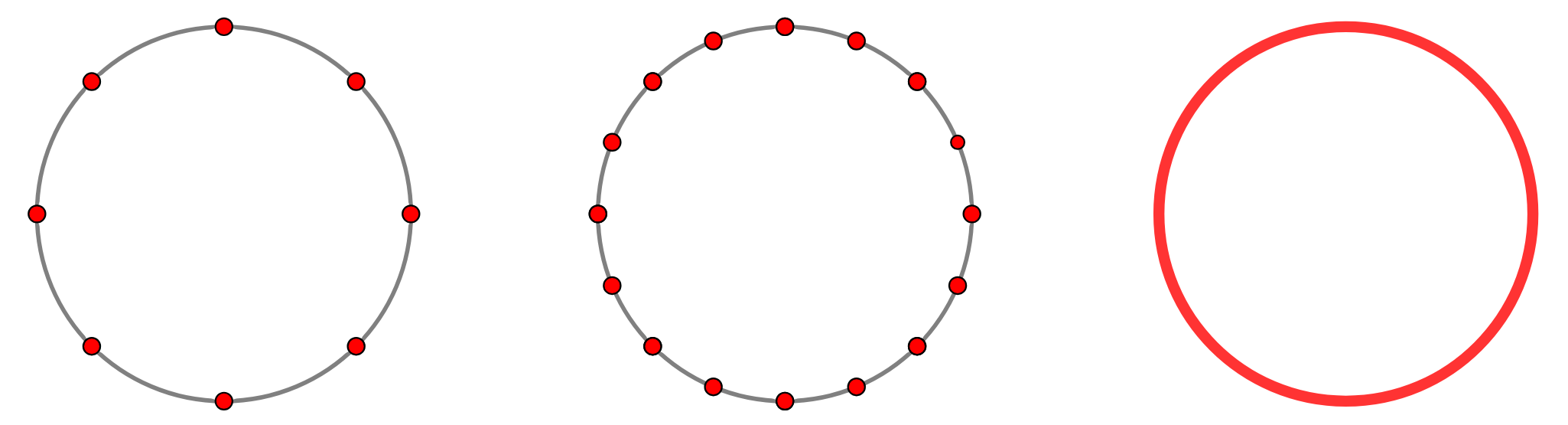
Figure 6: Fekete points for $n\in\{8,16\}$ and equilibrium measure with $K=\mathbb{U}$

Proof.

• Let $f$ be a continuous function. By applying the convergence theorem of Riemann sums to $\theta\mapsto f(e^{i\theta})$, we obtain :

  $$\nu(\mathbb{U}_{n})(f)=\frac{1}{n}\sum^{n-1}_{k=0}f(\exp{\frac{2ik\pi}{n}})\underset{n\rightarrow\infty}{\rightarrow}\int^{2\pi}_{0}f(e^{i\theta})\frac{\text{d}\theta}{2\pi}$$

  But $\mathbb{U}_{n}$ is a set of Fekete points of $\mathbb{U}$ (Prop. 2.2) therefore $\nu(\mathbb{U}_{n})\overset{*}{\longrightarrow}\mu_{\mathbb{U}}$ (Thm. 2.3). Hence $\boxed{\mu_{\mathbb{U}}=\frac{\text{d}\theta}{2\pi}}$.

• By making the substitution $t:=\theta+\phi$ :

  $$U^{\mu_{\mathbb{U}}}(z)=-\int^{2\pi}_{0}\log(\left\lvert z-e^{i\theta}\right\rvert)\frac{\text{d}\theta}{2\pi}=-\int^{2\pi}_{0}\log(\left\lvert ze^{i\phi}-e^{it}\right\rvert)\frac{\text{d}t}{2\pi}=U^{\mu_{\mathbb{U}}}(\left\lvert z\right\rvert)$$

  Let us consider $r\in\mathbb{R}_{+}$

  $$U^{\nu(\mathbb{U}_{n})}(r)=-\frac{1}{n}\log\left\lvert\prod^{n-1}_{k=0}(r-e^{\frac{2ik\pi}{n}})\right\rvert=-\frac{1}{n}\log\left\lvert r^{n}-1\right\rvert$$

  • If $r<1$, $\left\lvert r^{n}-1\right\rvert\rightarrow 1$, therefore $U^{\nu(\mathbb{U}_{n})}(r)=-\frac{1}{n}\log\left\lvert r^{n}-1\right\rvert\underset{n\rightarrow\infty}{\rightarrow}0$

  • If $r>1$, $U^{\nu(\mathbb{U}_{n})}(r)=-\frac{1}{n}\log\left\lvert r^{n}-1\right\rvert=-\log(r)-\frac{1}{n}\log\left\lvert\frac{1}{r}^{n}-1\right\rvert\underset{n\rightarrow\infty}{\rightarrow}-\log(r)$

  When $r\neq 1$, the function $t\in\mathbb{U}\mapsto-\log\left\lvert z-t\right\rvert\in\mathbb{C}$ is continuous, therefore
  $U^{\mu_{\mathbb{U}}}(r)=\displaystyle\lim_{n\rightarrow\infty}U^{\nu(\mathbb{U}_{n})}(r)=\begin{cases}0\text{ if }r<1\\ \log\frac{1}{r}\text{ if }r>1\end{cases}$
  When $r=1$, by using 2.2 and 2.3 we obtain : $0=-\log(\tau(\mathbb{U}))=V_{\mathbb{U}}=\int_{\mathbb{U}}U^{\mu_{\mathbb{U}}}(z)\ \mathrm{d}\mu_{\mathbb{U}}(z)=U^{\mu_{\mathbb{U}}}(1)$
  Hence $\boxed{U^{\mu_{\mathbb{U}}}(z)=-\log^{+}\left\lvert z\right\rvert}$

• From the proposition 2.4(c), it follows that $\mathrm{Cap}(\mathbb{U})=\mathrm{Cap}(\overline{B})$ and $V_{\overline{B}}=I(\mu_{\mathbb{U}})\neq+\infty$ thanks to the uniqueness of the equilibrium measure, hence $\mu_{\overline{B}}=\mu_{\mathbb{U}}$ and $U^{\mu_{\overline{B}}}=U^{\mu_{\mathbb{U}}}$.

∎

Now that we have unified the two notions of capacity previously defined, let us introduce a few properties of our capacity.

Proposition 2.4 

Let us consider $(K_{n})$ compact subsets of $\mathbb{C}$.

1. Let us consider $K_{1}\subset K_{2}$, then $\mathrm{Cap}(K_{1})\leq\mathrm{Cap}(K_{2})$.

2. Let us consider $\alpha,\beta\in\mathbb{C}$, then $\mathrm{Cap}(\alpha K+\beta)=\left\lvert\alpha\right\rvert\mathrm{Cap}(K)$.

3. $\mathrm{Cap}(K)=\mathrm{Cap}(\partial K)$.

4. Let us consider $(K_{n})_{n}$ a decreasing sequence and let us consider $K=\bigcap_{n}K_{n}$, then $\mathrm{Cap}(K)=\lim_{n}\mathrm{Cap}(K_{n})$.

5. Let us consider $(K_{n})_{n}$ an increasing sequence and let us assume that $K=\bigcup_{n}K_{n}$ is a compact set, then $\mathrm{Cap}(K)=\lim_{n}\mathrm{Cap}(K_{n})$.

6. Assume that $\mathrm{Cap}(K)=0$. Then $\nu(K)=0$, for all finite measures with compact support $\nu$ on $\mathbb{C}$ such that $I(\nu)<+\infty$. In particular, Lebesgue measure $m_{2}(K)=0$.

Proof. (a) and (b) are immediate consequences of the definition.

(c) results from theorem 2.3 and proposition 2.1.

(d) According to (a), it is enough to show that $\mathrm{Cap}(K)\geq\lim_{n}\mathrm{Cap}(K_{n})$, and moreover we can assume that $\mathrm{Cap}(K_{n})>0$ for all $n$. Let $\mu_{K_{n}}$ be the equilibrium measure of $K_{n}$, then $\mu_{E_{n}}\in\mathcal{P}(K_{0})$. According to Banach-Alaoglu-Bourbaki theorem, we can extract a sub-sequence $(\mu_{E_{\varphi(n)}})_{n}$ which converges weakly-* to a measure $\mu^{\star}\in\mathcal{P}(K_{0})$. Then lemma 2.2 gives us

$$I(\mu^{\star})\leq\liminf_{n}I(\mu_{\varphi(n)})=\liminf_{n}\left(-\log\mathrm{Cap}(K_{\varphi(n)})\right)=-\lim_{n}\log\mathrm{Cap}(K_{n})$$

On the other hand, Prop. LABEL:propSuppDecroi implies that

$$\operatorname{supp}\mu^{\star}\subset\bigcap_{n}\operatorname{supp}\mu_{E_{\varphi(n)}}\subset\bigcap_{n}K_{\varphi(n)}=\bigcap_{n}K_{n}=K$$

Therefore $\mu^{\star}\in\mathcal{P}(K)$, then

$$\mathrm{Cap}(K)\geq e^{-I(\mu^{\star})}\geq\exp\left(\lim_{n}\log\mathrm{Cap}(K_{n})\right)=\lim_{n}\mathrm{Cap}(K_{n})$$

(e) According to (a), it is enough to show that $\mathrm{Cap}(K)\leq\lim_{n}\mathrm{Cap}(K_{n})$, and moreover we can assume that $\mathrm{Cap}(K)>0$. Let us consider $\mu\in\mathcal{P}(K)$. Since $\lim_{n}\mu(K_{n})=\mu(K)=1$, we have $\mu(K_{n})>0$ for a sufficiently large $n$ . Then for such a $n$, we consider $\frac{\mu|_{K_{n}}}{\mu(K_{n})}\in\mathcal{P}(K_{n})$. We have

$$-\log\mathrm{Cap}(K_{n})\leq I\left(\frac{\mu|_{K_{n}}}{\mu(K_{n})}\right)=\frac{1}{\mu(K_{n})^{2}}\int_{K_{n}}\int_{K_{n}}\log\frac{1}{\left\lvert z-t\right\rvert}\ \mathrm{d}\mu(t)\ \mathrm{d}\mu(z)$$

Since the domain of integration $K_{n}\times K_{n}$ increases with $n$ and tends to $K\times K$, because $(K_{n})$ is increasing and tends to $K$, we obtain that

$$-\log\left(\lim_{n}\mathrm{Cap}(K_{n})\right)\leq\frac{1}{\lim_{n}\mu(K_{n})^{2}}\int_{K}\int_{K}\log\frac{1}{\left\lvert z-t\right\rvert}\ \mathrm{d}\mu(t)\ \mathrm{d}\mu(z)=I(\mu)$$

where we apply the monotone convergence theorem, after verifying that on $K\times K$, $\log\frac{1}{\left\lvert z-t\right\rvert}$ is lower bounded by $\log(1/\delta_{2}(K))$. In particular, when $\mu=\mu_{K}$ the equilibrium measure of $K$, $I(\mu_{K})=-\log\mathrm{Cap}(K)$, we obtain that $\mathrm{Cap}(K)\leq\lim_{n}\mathrm{Cap}(K_{n})$.

(f) Let $\nu$ be a measure verifying the theorem’s assumptions. If $\nu(K)>0$, then $\frac{\nu|_{K}}{\nu(K)}\in\mathcal{P}(K)$, therefore since $\mathrm{Cap}(K)=0$, we have

$$I\left(\frac{\nu|_{K}}{\nu(K)}\right)=\frac{1}{\nu(K)^{2}}\int_{K}\int_{K}\log\frac{1}{\left\lvert z-t\right\rvert}\ \mathrm{d}\nu(t)\ \mathrm{d}\nu(z)=+\infty$$

Then

$$I(\nu) =\iint\log\frac{1}{\left\lvert z-t\right\rvert}\ \mathrm{d}\nu(t)\ \mathrm{d}\nu(z)$$

$$=\left(\int\int_{(K\times K)^{c}}+\int_{K}\int_{K}\right)\log\frac{1}{\left\lvert z-t\right\rvert}\ \mathrm{d}\nu(t)\ \mathrm{d}\nu(z)$$

$$\geqslant\left(1-\nu(K)^{2}\right)\log\frac{1}{\delta_{2}(\operatorname{supp}(\nu))}+\nu(K)^{2}I\left(\frac{\nu|_{K}}{\nu(K)}\right)=+\infty$$

which is contradicted by $I(\nu)<+\infty$.

If $K\subset B(0,r)$, we have $m_{2}|_{B(0,r)}(\mathbb{C})=\pi r^{2}$ and $I(m_{2}|_{B(0,r)})<+\infty$. In fact, for all $z\in B(0,r)$,

$$\int_{B(0,r)}\log\frac{1}{\left\lvert z-t\right\rvert}\ \mathrm{d}m_{2}(t) \leq\int_{B(z,2r)}\log\frac{1}{\left\lvert z-t\right\rvert}\ \mathrm{d}m_{2}(t)$$

$$=\int_{0}^{2\pi}\int_{0}^{2r}\left(\log\frac{1}{\rho}\right)\rho\ \mathrm{d}\rho\leq 4\pi r\left\|\rho\log\rho\right\|_{L^{\infty}(]0,r])}<+\infty$$

Therefore we can apply what we have just proved to obtain that $m_{2}(K)=0$. ∎

Corollary 2.2 

Let $a=(a_{1}<\dots<a_{2n})$ be a set of strictly increasing real numbers. Let us consider $E_{a}=\displaystyle\bigcup_{k=0}^{n-1}[a_{2k+1},a_{2k+2}]$. The capacity of $E_{a}$ continuously varies with $a$.

Proof. Let us consider $d=\min_{i}\{a_{i+1}-a_{i}\}$ and $\varepsilon\in]0,d/2[$. Let

$$a_{\varepsilon,+}=(a_{1}-\varepsilon,a_{2}+\varepsilon,\dots a_{2n-1}-\varepsilon,a_{2n}+\varepsilon),\ a_{\varepsilon,-}=(a_{1}+\varepsilon,a_{2}-\varepsilon,\dots a_{2n-1}+\varepsilon,a_{2n}-\varepsilon),$$

We have $E_{a_{\varepsilon,-}}\subset E_{a}\subset E_{a_{\varepsilon,+}}$.

The left (resp. right) continuity of $\mathrm{Cap}(E_{a})$ with respect to $a$ is equivalent to $\mathrm{Cap}(E_{a})=\sup\mathrm{Cap}(E_{a_{\varepsilon,-}})$ (resp. $\mathrm{Cap}(E_{a})=\inf\mathrm{Cap}(E_{a_{\varepsilon,+}})$). These two conditions are insured by points (d) and (e) of the previous proposition.

∎

Definition 2.8 

Let $K\subset\mathbb{C}$ be a compact subset. Let us denote by $\Omega_{K}$ the unbounded connected component of $\mathbb{C}\backslash K$. Let us define the external boundary of a compact set $K\subset\mathbb{C}$ as the boundary of $\Omega_{K}$, subset of $\mathbb{C}$:

$$\partial_{\infty}K:=\partial\Omega_{K}$$

and the essential closure as the complement of $\Omega_{K}$ with respect to $\mathbb{C}$:

$$K^{ce}:=\mathbb{C}\backslash\Omega_{K}$$

Corollary 2.3 

Let $K\subset\mathbb{C}$ be a compact set, then:

1. If $\mathring{K}$ is non-empty, then $\mathrm{Cap}(K)>0$; in other words, $\mathrm{Cap}(K)=0$ implies that $K=\partial K$;

2. $\Omega_{K}=\Omega_{\partial K}=\Omega_{\partial_{\infty}K}=\Omega_{K^{ce}}$;

3. $\partial_{\infty}K=\partial K^{ce}$, $K^{ce}\supset K\supset\partial_{\infty}K$;

4. $\mathrm{Cap}(K^{ce})=\mathrm{Cap}(\partial_{\infty}K)=\mathrm{Cap}(K)=\mathrm{Cap}(\partial K)$.

5. Let $\mu_{K}$ be the equilibrium measure of $K$. If $\mathrm{Cap}(K)>0$, then $\operatorname{supp}(\mu_{K})\subset\partial_{\infty}K$ and $\mu_{K}=\mu_{K^{ce}}=\mu_{\partial_{\infty}K}$.

6. Let $(K_{n})$ be an increasing sequence of compact subsets of $\mathbb{C}$, and $B=\bigcup_{n}K_{n}$. Then $\mathrm{Cap}(B)=\lim_{n}\mathrm{Cap}(K_{n})$.

Proof. (a) results from Prop. 2.4 (f) using Lebesgue measure.

(b) and (c) result from the definition.

(d) can be deduced from (c) and Prop. 2.4 (a),(c). And (e) results from it, given the uniqueness (Thm. 2.2).

(f) Let us suppose $K_{n}$ of finite capacity. Let $K\subset B$ be a compact. Then $(K\cap K_{n})$ is an increasing sequence that converges to $K$, then we have

$$\mathrm{Cap}(K)=\lim_{n}\mathrm{Cap}(K\cap K_{n})$$

hence $\mathrm{Cap}(B)\leq\lim_{n}\mathrm{Cap}(K_{n})$. The other inequality is trivial. ∎

2.3  Potentials and semi harmonic functions

For some probability measure $\mu$, the associated potential $U^{\mu}$ is a function of a complex variable belonging to a specific family of functions: semi-harmonic functions. These are semi-continuous functions which verify the maximum/minimum modulus principle. Notions on these functions are provided in the appendix LABEL:appendixeSemiharmonic.

By using properties of these functions, we will prove several important results on potentials and capacities. First, we will prove Frostman’s theorem (Thm. 2.5) which states that the equilibrium potential of a compact set $K$ has the shape of a platter on $K$. Secondly we will prove theorem 2.8 which states that under a few assumptions of regularity, a holomorphic function transforms the capacity of a compact set according to its monomial of highest degree. This theorem and its two corollaries 2.10, 2.11, provide a useful tool to calculate some capacities.

A few technical proofs are gathered in the appendix LABEL:appendixthmPrincpMaxPotent.

2.3.1  Frostman’s theorem

To begin with, let us remind ourselves of the definition of semi-harmonic functions and give two important examples of super-harmonic functions.

Definition 2.9  ((super-,sub-)harmonic functions). 

Let $D\subset\mathbb{C}$ be an open set. A function $f:D\to\mathbb{R}$ is called harmonic (resp. super-harmonic, sub-harmonic) if it is continuous (resp. lower semi-continuous, upper semi-continuous) and if it verifies the mean value property (resp. super-mean, sub-mean): for all $z\in D$, if the disk $\{\left\lvert\zeta-z\right\rvert\leq r\}\subset D$, we have

$$f(z)=\frac{1}{2\pi}\int_{0}^{2\pi}f(z+re^{i\theta})\ \mathrm{d}\theta\quad(\emph{resp}.\;\geq,\leq)$$

Example 2.6 

$g(z)=\log\frac{1}{\left\lvert z-t\right\rvert}$ is superharmonic and harmonic at points $z\neq t$. ∎

Example 2.7 

Let $\mu$ be a positive measure with compact support $K$, then the potential

$$U^{\mu}(z)=\int\log\frac{1}{\left\lvert z-t\right\rvert}\ \mathrm{d}\mu(t)$$

is superharmonic on $\mathbb{C}$ and harmonic on $\mathbb{C}\backslash K$.

Proof. $U^{\mu}$ is lower semi-continuous since $\log\frac{1}{\left\lvert z-t\right\rvert}$ is for all $t$. By using Fubini-Tonelli theorem, we obtain

$$\frac{1}{2\pi}\int_{0}^{2\pi}U^{\mu}(z+re^{i\theta})\ \mathrm{d}\theta=\int\frac{1}{2\pi}\int_{0}^{2\pi}\log\frac{1}{\left\lvert z+re^{i\theta}-t\right\rvert}\ \mathrm{d}\theta\ \mathrm{d}\mu(t).$$

The example 2.6 gives us that this last integral is smaller than $\displaystyle\int\log\frac{1}{\left\lvert z-t\right\rvert}\ \mathrm{d}\mu(t)=U^{\mu}(z)$. Therefore, $U^{\mu}$ is superharmonic on $\mathbb{C}$. By considering $z\notin K$ and $r<\mathrm{dist}(z,K)$, it follows from example 2.6 that this last integral is equal to $U^{\mu}(z)$, hence the harmonicity. ∎

Theorem 2.4  (Maximum principle for potentials). 

Let $\mu$ be a finite positive measure with compact support. If $U^{\mu}(z)\leq M$ for all $z\in\operatorname{supp}(\mu)$, then the same goes for all $z\in\mathbb{C}$.

The proof is given in the appendix LABEL:appendixeSemiharmonic, Corollary LABEL:appendixthmPrincpMaxPotent.

Let us state and prove an important theorem on equilibrium potentials : Frostman’s theorem, which claims that the equilibrium potential has the shape of a platter and is upper bounded every where by Robin’s constant (cf. Figure 7).

Theorem 2.5  (Frostman). 

Let $K$ be a compact subset of $\mathbb{C}$ such that $\mathrm{Cap}(K)>0$, then

1. $U^{\mu_{K}}(z)\leqslant V_{K}$ for all $z\in\mathbb{C}$

2. $U^{\mu_{K}}(z)=V_{K}$ for all $z\in K-S$ where $\mathrm{Cap}(S)=0$

3. $U^{\mu_{K}}(z)<V_{K}$ for all $z\in\Omega$ where $\Omega$ is the non bounded connected component of $\mathbb{C}-K$

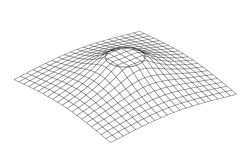
Figure 7: Frostman’s theorem

Proof. The formal argument proceeds in three steps. First of all, let us define for $n\geq 1$ the following sets: $K_{n}=\left\{z\in K|U^{\mu_{K}}\leq V_{K}-1/n\right\}$ and $L_{n}=\left\{z\in\operatorname{support}\left(\mu_{K}\right)|U^{\mu_{K}}(z)>V_{K}+1/n\right\}$. We will first show that the $K_{n}$ have capacity zero, then that the $L_{n}$ are empty, and we will finally conclude, using the maximum principle for potentials (2.4).

Let us argue by contradiction to prove that $\operatorname{Cap}(K_{n})=0$. Assume there exists $n\geq 1$ such that $\operatorname{Cap}(K_{n})>0$. We remind that $V_{K}=I\left(\mu_{K}\right)=\int U^{\mu_{K}}d\mu_{K}$, therefore, there exists some $z_{0}$ in the support of $\mu_{K}$ verifying $U^{\mu_{K}}\left(z_{0}\right)\geq V_{K}$. By using the lower semi-continuity of $U^{\mu_{K}}$, there exists a closed ball denoted by $B$ with radius $r>0$ and center $z_{0}$, on which we have $U^{\mu_{K}}(z)>V_{K}-1/2n$. Then, we have $B\cap K_{n}=\emptyset$, and $\mu_{K}(B)=a>0$ because $z_{0}$ is in the support of $\mu_{K}$. To get a contradiction, we want to build a measure that contradicts the fact that $V_{K}$ is minimal. To do so, we use the assumption that $\operatorname{Cap}(K_{n})>0$. In fact, we can consider a measure $\mu$ on $K_{n}$ such that $I(\mu)$ is finite. We then build the following measure:

$$\sigma=\left\{\begin{array}[]{ll}{\mu,}&{\text{ on }K_{n}}\\ {-\mu_{K}/a,}&{\text{ on }B}\\ {0,}&{\text{ on the rest }}\end{array}\right.$$

Let us then consider the family of probability measures $\mu_{t}=\mu_{K}+t\sigma$ for $t\in]0;a[$. Given how we built $B$, we obtain :

$$I\left(\mu_{K}\right)-I\left(\mu_{t}\right)\geq 2t\left(V_{K}-1/2n-V_{K}+1/n\right)+O\left(t^{2}\right)$$

Therefore for all $t$ sufficiently close to $0$ (we remind that here $n$ is fixed), we have $I\left(\mu_{K}\right)=V_{K}\geq I\left(\mu_{t}\right)$, which contradicts the fact that $\mu_{K}$ is minimal since here , $\mu_{t}\neq\mu_{K}$.

Secondly, let us show by contradiction that $L_{n}=\emptyset$. If one of the $L_{n}$ is non-empty, using the same argument as earlier, there exists a closed ball $\tilde{B}$ on which $U^{\mu_{K}}(z)>V_{K}+1/n$. As we did earlier, we consider $\tilde{a}=\mu_{K}(\tilde{B})>0$. According to the previous point, we obtain for all $n$, $\mu_{K}(K_{n})=0$, therefore, $U^{\mu_{K}}(z)\geq V_{K}$ except on a set with measure zero. We then have :

$$V_{K}=I\left(\mu_{K}\right) =\int_{K}U^{\mu_{K}}d\mu_{K}$$

$$=\int_{\tilde{B}}U^{\mu_{K}}d\mu_{K}+\int_{K\backslash\tilde{B}}U^{\mu_{K}}d\mu_{K}$$

$$\geq\left(V_{K}+\frac{1}{n}\right)\tilde{a}+V_{K}(1-\tilde{a})>V_{K}$$

We obtain a contradiction, and the $L_{n}$ are empty.

These two facts allow us to prove the three claims of the theorem : since all the $L_{n}$ are empty, we have the inequality of the first claim on the support of $\mu_{K}$, therefore, on $\mathbb{C}$, thanks to the maximum principle. The second claim results from the fact that $\operatorname{Cap}(\bigcup_{n}K_{n})=0$ which gives us that $U^{\mu_{K}}(z)\geq V_{K}$ on $K\backslash\bigcup_{n}K_{n}$, and from the first claim which states that $U^{\mu_{K}}(z)\leq V_{K}$. Finally, the last claim results from the harmonicity of $U^{\mu_{K}}$ on $\Omega$.

∎

Example 2.8 

When $K=\mathbb{U}$ (Prop. 2.5), the potential $U^{\mu_{\mathbb{U}}}(z)=\begin{cases}0=V_{\mathbb{U}}\text{ if }\left\lvert z\right\rvert\leqslant 1\\ \log(\frac{1}{\left\lvert z\right\rvert})\text{ if }\left\lvert z\right\rvert>1\end{cases}$ verifies Frostman’s theorem with $S=\emptyset$.

Corollary 2.4 

Let $K\subset\mathbb{C}$ be a compact set with $\mathrm{Cap}(K)>0$ and $\mu_{K}$ its equilibrium measure. Then $U^{\mu_{K}}\equiv V_{K}$ in the interior of $K$. Moreover, since $\mu_{K}=\mu_{K^{ce}}$ (Cor. 2.3(e)), we have $U^{\mu_{K}}\equiv V_{K}$ in the interior of $K^{ce}$.

Proof. Frostman’s theorem implies that

$$U^{\mu_{K}}(z)=V_{K},\quad q-a.e.\text{~{}in~{}}\partial K$$

On the other hand, $U^{\mu_{K}}$ is superharmonic and lower bounded by $\log(1/d_{2}(K))$ in $K$. Then the maximum principle can be applied to $U^{\mu_{K}}$ on each connected component of $\mathring{K}$ to obtain $U^{\mu_{K}}\geq V_{K}$ in $\mathring{K}$. However, Frostman’s theorem already gives us an upper bound, $V_{K}$. Therefore $U^{\mu_{K}}=V_{K}$ in $\mathring{K}$.

∎

2.3.2  Calculation of capacities

The goal of this section is theorem 2.8, which states that a holomorphic function transforms the capacity according to its monomial of highest degree, and two corollaries which serve as tools to calculate some capacities.

The main tool of this proof is Green’s function with respect to a compact set.

Theorem 2.6 

Let $K\subset\mathbb{C}$ be a compact set with $\mathrm{Cap}(K)>0$ and $\Omega_{K}$ the non bounded connected component of $\mathbb{C}\backslash K$. Then there exists a unique function $g_{K}(\cdot,\infty):\Omega_{K}\to\mathbb{R}$ characterized by the following properties:

1. $g_{K}(\cdot,\infty)$ is harmonic on $\Omega_{K}$ and bounded outside of all the neighborhoods of $\infty$;

2. $g_{K}(\cdot,\infty)-\log\left\lvert\cdot\right\rvert$ is bounded on a neighborhood of $\infty$;

3. $\lim_{z\to\zeta}g_{K}(z,\infty)=0$ q-a.e. in $\partial\Omega_{K}$.

Proof. The existence is given by Frostman’s theorem and example 2.7 if we consider

$$g_{K}(z,\infty)=V_{K}-U^{\mu_{K}}(z).$$ (1)

Let $g,g^{\prime}$ be two functions verifying these three properties, then $g-g^{\prime}$ is harmonic and bounded on $\Omega_{K}$, and therefore can be extended to a harmonic function on $\Omega_{K}\cup\{\infty\}$. According to the second point, we have $g(z)>0$ (resp. $g^{\prime}(z)>0$) for $R\gg 0$ so that $K\subset B(0,R)$; the minimum principle applied on $\Omega_{K}\cap B(0,R)$ gives us that $g(z)>0$ (resp. $g^{\prime}(z)>0$) on $\Omega_{K}\cap B(0,R)$, and then on $\Omega_{K}$. The uniqueness results from the third property and the minimum principle applied twice on $\Omega_{K}\cup\{\infty\}$ to $g(z)-g^{\prime}(z)$ and $g^{\prime}(z)-g(z)$ respectively. ∎

Definition 2.10 

Let us denote by $g_{K}(\cdot,\infty):\Omega_{K}\to\mathbb{R}$ the Green’s function with respect to $K$, with a pole at infinity.

Corollary 2.5 

Let $K\subset\mathbb{C}$ be a compact set such that $\mathrm{Cap}(K)>0$. We then have $g_{K}(\cdot,\infty)>0$ on $\Omega_{K}$.

Corollary 2.6 

If two compact sets $K_{1},K_{2}\subset\mathbb{C}$ are such that $\mathrm{Cap}(K_{1})>0$ or $\mathrm{Cap}(K_{2})>0$, and that $\Omega_{K_{1}}=\Omega_{K_{2}}$, then

$$g_{K_{1}}(\cdot,\infty)=g_{K_{2}}(\cdot,\infty).$$

In particular, let $K\subset\mathbb{C}$ be a compact set with $\mathrm{Cap}(K)>0$, then

$$g_{K}(\cdot,\infty)=g_{\partial K}(\cdot,\infty)=g_{\partial_{\infty}K}(\cdot,\infty)=g_{K^{ce}}(\cdot,\infty).$$

Proof. Note that the three claims in Thm. 2.6 only depend on $\Omega_{K}$, the non bounded connected component of $\mathbb{C}\backslash K$ ; therefore the result immediately follows from the definition and Cor. 2.3. ∎

Theorem 2.7 

Let $K\subset\mathbb{C}$ be a compact set with $\mathrm{Cap}(K)>0$ and $g_{K}(\cdot,\infty)$ Green’s function with respect to $K$, with a pole at infinity. Then

1. $g_{K}(z,\infty)=\log\left\lvert z\right\rvert+V_{K}+o_{z\to\infty}(1)$;

2. The equilibrium potential of $K$ is $U^{\mu_{K}}=V_{K}-g_{K}(\cdot,\infty)$; then (Thm. 2.5) $g_{K}(\cdot,\infty)>0$ on $\Omega_{K}$.

Proof. It immediately results from the formula (1) given in the proof of theorem 2.6 and in the definition of the potential $U^{\mu_{K}}$. ∎

Let us define the notion of regularity of a compact set. We will see later that it is the right assumption to link the capacity of two compact sets and thanks to Prop 2.7, it is a special case that will be useful in a more general approach.

Definition 2.11 

Let $K\subset\mathbb{C}$ be a compact set such that $\mathrm{Cap}(K)>0$. We call $\zeta_{0}\in\partial\Omega_{K}$ a regular point if

$$\lim_{\Omega_{K}\ni z\to\zeta_{0}}U^{\mu_{K}}(z)=V_{K};$$

otherwise, we write that $\zeta_{0}$ is an irregular point. We write that $\Omega_{K}$ is a regular set if all the points of $\partial\Omega_{K}$ are regular.

According to the relation between the potential and Green’s function (Thm. 2.7), we have the following property :

Corollary 2.7 

A point $\zeta_{0}\in\partial\Omega_{K}$ is regular if and only if $\lim_{z\to\zeta_{0}}g_{K}(z,\infty)=0$.

Proposition 2.5 

Let $K\subset\mathbb{C}$ be a compact set such that $\mathrm{Cap}(K)>0$. Then $U^{\mu_{K}}(\zeta_{0})=V_{K}$ implies the continuity of $U^{\mu_{K}}$ at point $\zeta_{0}$. The reciprocal implication is true if $\zeta_{0}\in\operatorname{supp}(\mu_{K})$.

Proof. It follows from the semi-continuity of $U^{\mu_{K}}$ and Frostman’s theorem that:

$$U^{\mu_{K}}(\zeta_{0})\leq\liminf_{z\to\zeta_{0}}U^{\mu_{K}}(z)\leq\limsup_{z\to\zeta_{0}}U^{\mu_{K}}(z)\leq V_{K}.$$

Therefore if $U^{\mu_{K}}(\zeta_{0})=V_{K}$, $U^{\mu_{K}}$ is continuous at point $\zeta_{0}$.

Conversely, if $U^{\mu_{K}}$ is continuous at point $\zeta_{0}$ and $U^{\mu_{K}}(\zeta_{0})<V_{K}$, then there exists $r>0$ such that $U^{\mu_{K}}<V_{K}$ on $\overline{B(\zeta_{0},r)}$, therefore according to Frostman’s theorem, $\mathrm{Cap}(\overline{B(\zeta_{0},r)})\cap K)\leq\mathrm{Cap}(S)=0$, then according to Prop. 2.4(f), we have

$$\mu_{K}(\overline{B(\zeta_{0},r)}\cap K)=0.$$

Therefore $\mu_{K}(\overline{B(\zeta_{0},r)})=0$ and we deduce from it that $\zeta_{0}\notin\operatorname{supp}(\mu_{K})$. ∎

Corollary 2.8 

Let us consider $\zeta_{0}\in\operatorname{supp}(\mu_{K})$ then for all $r>0$, $\mathrm{Cap}(B(\zeta_{0},r)\cap K)>0$.

Proof. It is indeed the contrapositive of the last argument of the previous proof. ∎

Corollary 2.9 

The set of all irregular points has capacity zero.

Proof. Let us assume that $\mathrm{Cap}(K)>0$. Then the corollary results from Frostman’s theorem. ∎

To get a sufficient condition of regularity, let us introduce the following notion:

Definition 2.12 

Let us consider $\Omega\subset\mathbb{C}$. We write that $\Omega$ verifies the cone condition if for all $\zeta\in\partial\Omega$, there exists $\zeta_{1}\neq\zeta$ such that the segment $[\zeta,\zeta_{1}]\subset\mathbb{C}\backslash\Omega$.

Proposition 2.6 

Let $K\subset\mathbb{C}$ be a compact set with $\mathrm{Cap}(K)>0$. If $\Omega_{K}$ verifies the cone condition, then $\Omega_{K}$ is a regular set.

The proof is given in appendix LABEL:propConditionConeRegProof.

The following proposition will be useful in order to consider the domain regular.

Proposition 2.7 

Let $K\subset\mathbb{C}$ be a non-empty compact set and let $K^{\epsilon}=\{z\in\mathbb{C}:\mathrm{dist}(z,K)\leq\epsilon\}$. Then $\mathrm{Cap}(K^{\epsilon})>0$ and $\Omega_{K^{\epsilon}}$ verifies the cone condition, therefore $\Omega_{K^{\epsilon}}$ is regular.

Proof. Since the interior of $K^{\epsilon}$ is non-empty, we have $\mathrm{Cap}(K^{\epsilon})>0$. Moreover, by definition, all points $\zeta$ in $\partial K^{\epsilon}$ are exactly at a distance of $\epsilon$ from $K$, therefore there exists $\zeta_{1}\in K$ such that $[\zeta,\zeta_{1}]\subset K^{\epsilon}\subset\mathbb{C}\backslash\Omega_{K}$. ∎

We will now prove a few results that allow us to compare the capacity of two compact sets thanks to holomorphic functions and the notion of regularity previously defined.

Lemma 2.3 

Let $f$ be a non locally constant holomorphic function defined at $\infty$ by $f(\infty)=\infty$. Then there exists some integer $n\in\mathbb{N}^{*}$ and some $A\neq 0$ such that

$$f(z)\sim Az^{n},\quad z\to\infty$$

$$\log\left\lvert f(z)\right\rvert=n\log\left\lvert z\right\rvert+\log\left\lvert A\right\rvert+o(1),\quad z\to\infty$$

Let us define $A_{f}=A,n_{f}=\operatorname{ord}_{\infty}(f)=n$. ∎

Theorem 2.8 

Let $K_{1},K_{2}\subset\mathbb{C}$ be two non-empty compact sets. Let $f:\Omega_{K_{1}}\cup\{\infty\}\to\Omega_{K_{2}}\cup\{\infty\}$ be a non constant holomorphic function such that $f(\infty)=\infty$. Then,

1. $\left\lvert A_{f}\right\rvert\mathrm{Cap}(K_{1})^{n_{f}}\geq\mathrm{Cap}(K_{2})$.

2. Moreover assume that :

   1. $\mathrm{Cap}(K_{2})>0$;

   2. $f^{-1}(\infty)=\{\infty\}$;

   3. $\Omega_{K_{2}}$ is regular;

   4. $f$ can be continuously extended to the boundaries $\partial\Omega_{K_{1}}\to\partial\Omega_{K_{2}}.$

   Then, $\mathrm{Cap}(K_{1})$>0, $\Omega_{K_{1}}$ is a regular set and

   $$g_{K_{1}}(\cdot,\infty)=\frac{1}{n_{f}}g_{K_{2}}(f(\cdot),\infty)$$

   $$\left\lvert A_{f}\right\rvert\mathrm{Cap}(K_{1})^{n_{f}}=\mathrm{Cap}(K_{2}).$$

The complete proof is provided in the appendix LABEL:appendixthmPrincpMaxPotent.

To understand how to apply this theorem, let us see when the conditions in $(b)$ are verified:

(ii) holds when $f$ is biholomorphic, or when $f$ is a polynomial;

(iii) holds when $\Omega_{K}$ verifies the cone condition (Prop. 2.6).

We therefore have the two following corollaries (by applying the same technique as in Prop. 2.7 if necessary):

Corollary 2.10 

If $f$ is biholomorphic, we have $n_{f}=n_{f^{-1}}=1$ and $A_{f}A_{f^{-1}}=1$; Let us apply (a) twice to obtain (with notation $f^{\prime}(\infty)=A_{f}$)

$$\left\lvert f^{\prime}(\infty)\right\rvert\mathrm{Cap}(K_{1})=\mathrm{Cap}(K_{2}).$$

∎

Corollary 2.11 

Assume that $f$ is a polynomial function of degree $n$:

$$f(z)=\sum_{i=0}^{n}a_{i}x^{i},\quad a_{n}\neq 0.$$

Let $K\subset\mathbb{C}$ be a compact set. Then

$$\left\lvert a_{n}\right\rvert\mathrm{Cap}(f^{-1}(K))^{n}=\mathrm{Cap}(K).$$

Proof. Assume that $K\neq\emptyset$. Let us try to apply theorem 2.8 (b). Since $f$ is a polynomial function, (ii) is verified for all compacts in $\mathbb{C}$. For $\epsilon>0$, let us consider $K^{\epsilon}=\{z\in\mathbb{C}:\mathrm{dist}(z,K)\leq\epsilon\}$. Let us show that the conditions (i),(iii),(iv) of the theorem are verified for the compact sets $f^{-1}(K^{\epsilon})$ and $K^{\epsilon}$ and that $f(\Omega_{f^{-1}(K^{\epsilon})})\subset\Omega_{K^{\epsilon}}$; It will result in

$$\left\lvert a_{n}\right\rvert\mathrm{Cap}(f^{-1}(K^{\epsilon}))^{n}=\mathrm{Cap}(K^{\epsilon}).$$

When $\epsilon\to 0$, it allows us to conclude.

(i) $K^{\epsilon}$ has a non-empty interior, therefore $\mathrm{Cap}(K^{\epsilon})>0$ (Cor. 2.3).

(iii) results from Prop. 2.6 and Prop. 2.7.

(iv) We will actually prove this claim for all compact sets $K$ (instead of $K^{\epsilon}$). A topological analysis shows that $f(\partial f^{-1}(K))=\partial K$. We have left to prove that $f(\partial\Omega_{f^{-1}(K)})\subset\partial\Omega_{K}$. We have $f(\infty)=\infty$ and $K$ a compact set, therefore $f^{-1}(K)$ is a compact set; likewise, the inverse image of each (open) bounded connected component of $\mathbb{C}\backslash K$ is bounded, therefore included in one of the bounded component of $\ f^{-1}(K)$. Therefore $\Omega_{f^{-1}(K)}\subset f^{-1}(\Omega_{K})$, then

$$f(\Omega_{f^{-1}(K)})\subset\Omega_{K}$$

$$f(\partial\Omega_{f^{-1}(K)})\subset\overline{\Omega_{K}}.$$

We finally obtain that

$$f(\partial\Omega_{f^{-1}(K)})\subset\overline{\Omega_{K}}\cap\partial K=\partial\Omega_{K},$$

which allows us to apply theorem 2.8 (b) to obtain the final result. ∎

2.4  Chebyshev constant

Let us now give a third equivalent definition of the capacity, defined thanks to Chebyshev polynomials. This point of view is very useful to calculate the capacity of segments of $\mathbb{R}$.

First, let us state the equioscillation theorem :

Theorem 2.9  (Equioscillation). 

Let us consider $n\in\mathbb{N}$. Let $f$ be a continuous function on $[a,b]$. Let us consider $P\in\mathbb{R}_{n}[X]$. $P$ minimizes $||f-P||_{\infty,[a,b]}$ if and only if there exists $n+2$ points $a\leqslant x_{0}<x_{1}<\dots x_{n+1}\leqslant b$ such that $f(x_{i})-P(x_{i})=\pm(-1)^{i}||f-P||_{\infty,[a,b]}$

The proof of this theorem is not that hard but is quite long. In order not to overfill this paper, we advise the reader to read article [equioscillation] for a complete and illustrated proof.

Definition 2.13  (The Chebyshev constant). 

Let us consider some $n\in\mathbb{N}$ and $K$ a compact subset of $\mathbb{C}$, let us denote by $||\cdot||_{K}$ the uniform norm on $K$ and :

$$t_{n}(K)=\displaystyle\inf_{P\in\mathbb{C}_{n-1}[X]}||X^{n}+P||_{K}.$$

If $K$ contains an infinite number of points, there exists a unique monic polynomial $T_{n}\in\mathbb{R}_{n}[X]$, called Chebyshev polynomial such that $t_{n}(K)=||T_{n}||_{K}$.

Let us define the Chebyshev constant as follows :

$$\mathrm{Cheb}(K)=\lim_{n\rightarrow+\infty}t_{n}(K)^{\frac{1}{n}}.$$

Proof.

• If $K$ is an infinite set, $||\cdot||_{K}$ is a norm on $\mathbb{C}[X]$. The existence of $T_{n}$ follows from the fact that the distance to a closed vector subspace is reached. The uniqueness follows from the reciprocal implication of the equioscillation theorem (2.9).

• Let us consider $n,m\in\mathbb{N}$. Since $T_{n}T_{m}$ is a monic polynomial of degree $n+m$, we have

  $$||T_{n+m}||_{K}=\displaystyle\inf_{\begin{subarray}{c}P\in\mathbb{C}_{n+m}[X]\\ \text{monic}\end{subarray}}||P||_{K}\leqslant||T_{n}T_{m}||_{K}\leqslant||T_{n}||_{K}||T_{m}||_{K}$$

  Therefore $t_{n+m}(K)\leqslant t_{n}(K)t_{m}(K)$ and $(\log(t_{n}(K)))_{n\in\mathbb{N}}$ is sub-additive. It follows from the sub-additivity lemma that $(\frac{1}{n}\log(t_{n}(K)))_{n\in\mathbb{N}}$ converges, which proves that $\mathrm{Cheb}(K)$ is well defined.

∎

The Chebyshev constant is equivalent to the logarithmic capacity and the transfinite diameter :