Transferring Robustness for Graph Neural Network Against Poisoning Attacks

Abstract.

Graph neural networks (GNNs) are widely used in many applications. However, their robustness against adversarial attacks is criticized. Prior studies show that using unnoticeable modifications on graph topology or nodal features can significantly reduce the performances of GNNs. It is very challenging to design robust graph neural networks against poisoning attack and several efforts have been taken. Existing work aims at reducing the negative impact from adversarial edges only with the poisoned graph, which is sub-optimal since they fail to discriminate adversarial edges from normal ones. On the other hand, clean graphs from similar domains as the target poisoned graph are usually available in the real world. By perturbing these clean graphs, we create supervised knowledge to train the ability to detect adversarial edges so that the robustness of GNNs is elevated. However, such potential for clean graphs is neglected by existing work. To this end, we investigate a novel problem of improving the robustness of GNNs against poisoning attacks by exploring clean graphs. Specifically, we propose PA-GNN, which relies on a penalized aggregation mechanism that directly restrict the negative impact of adversarial edges by assigning them lower attention coefficients. To optimize PA-GNN for a poisoned graph, we design a meta-optimization algorithm that trains PA-GNN to penalize perturbations using clean graphs and their adversarial counterparts, and transfers such ability to improve the robustness of PA-GNN on the poisoned graph. Experimental results on four real-world datasets demonstrate the robustness of PA-GNN against poisoning attacks on graphs. Code and data are available here: https://github.com/tangxianfeng/PA-GNN.

1. Introduction

Graph neural networks (GNNs) (Kipf and Welling, 2016; Hamilton et al., 2017), which explore the power of neural networks for graph data, have achieved remarkable results in various applications (Veličković et al., 2017; Fan et al., 2019; Huang et al., 2019). The key to the success of GNNs is its signal-passing process (Wu et al., 2019c), where information from neighbors is aggregated for every node in each layer. The collected information enriches node representations, preserving both nodal feature characteristics and topological structure.

Though GNNs are effective for modeling graph data, the way that GNNs aggregate neighbor nodes’ information for representation learning makes them vulnerable to adversarial attacks (Zügner et al., 2018; Zügner and Günnemann, 2019; Dai et al., 2018; Wu et al., 2019b; Xu et al., 2019a). Poisoning attack on a graph (Zügner et al., 2018), which adds/deletes carefully chosen edges to the graph topology or injects carefully designed perturbations to nodal features, can contaminate the neighborhoods of nodes, bring noises/errors to node representations, and degrade the performances of GNNs significantly. The lack of robustness become a critical issue of GNNs in many applications such as financial system and risk management (Akoglu et al., 2015). For example, fake accounts created by a hacker can add friends with normal users on social networks to promote their scores predicted by a GNN model. A model that’s not robust enough to resist such “cheap” attacks could lead to serious consequences. Hence, it is important to develop robust GNNs against adversarial attacks. Recent studies of adversarial attacks on GNNs suggest that adding perturbed edges is more effective than deleting edges or adding noises to node features (Wu et al., 2019b). This is because node features are usually high-dimensional, requiring larger budgets to attack. Deleting edges only result in the loss of some information while adding edges is cheap to contaminate information passing dramatically. For example, adding a few bridge edges connecting two communities can affect the latent representations of many nodes. Thus, we focus on defense against the more effective poisoning attacks that a training graph is poisoned with injected adversarial edges.

To defend against the injected adversarial edges, a natural idea is to delete these adversarial edges or reduce their negative impacts. Several efforts have been made in this direction (Zhu et al., 2019; Wu et al., 2019b; Jin et al., 2019). For example, Wu et al. (Wu et al., 2019b) utilize Jaccard similarity of features to prune perturbed graphs with the assumption that connected nodes have high feature similarity. RGCN in (Zhu et al., 2019) introduce Gaussian constrains on model parameters to absorb the effects of adversarial changes. The aforementioned models only rely on the poisoned graph for training, leading to sub-optimal solutions. The lack of supervised information about real perturbations in a poisoned graph obstructs models from modeling the distribution of adversarial edges. Therefore, exploring alternative supervision for learning the ability to reduce the negative effects of adversarial edges is promising.

There usually exist clean graphs with similar topological distributions and attribute features to the poisoned graph. For example, Yelp and Foursquare have similar co-review networks where the nodes are restaurants and two restaurants are linked if the number of co-reviewers exceeds a threshold. Facebook and Twitter can be treated as social networks that share similar domains. It is not difficult to acquire similar graphs for the targeted perturbed one. As shown in existing work (Shu et al., 2018; Lee et al., 2017), because of the similarity of topological and attribute features, we can transfer knowledge from source graphs to target ones so that the performance on target graphs is elevated. Similarly, we can inject adversarial edges to clean graphs as supervisions for training robust GNNs, which are able to penalize adversarial edges. Such ability can be further transferred to improve the robustness of GNNs on the poisoned graph. Leveraging clean graphs to build robust GNNs is a promising direction. However, prior studies in this direction are rather limited.

Therefore, in this paper, we investigate a novel problem of exploring clean graphs for improving the robustness of GNNs against poisoning attacks. The basic idea is first learning to discriminate adversarial edges, thereby reducing their negative effects, then transferring such ability to a GNN on the poisoned graph. In essence, we are faced with two challenges: (i) how to mathematically utilize clean graphs to equip GNNs with the ability of reducing negative impacts of adversarial edges; and (ii) how to effectively transfer such ability learned on clean graphs to a poisoned graph. In an attempt to solve these challenges, we propose a novel framework Penalized Aggregation GNN (PA-GNN). Firstly, clean graphs are attacked by adding adversarial edges, which serve as supervisions of known perturbations. With these known adversarial edges, a penalized aggregation mechanism is then designed to learn the ability of alleviating negative influences from perturbations. We further transfer this ability to the target poisoned graph with a special meta-optimization approach, so that the robustness of GNNs is elevated. To the best of our knowledge, we are the first one to propose a GNN that can directly penalize perturbations and to leverage transfer learning for enhancing the robustness of GNN models. The main contributions of this paper are:

• We study a new problem and propose a principle approach of exploring clean graphs for learning a robust GNN against poisoning attacks on a target graph;

• We provide a novel framework PA-GNN, which is able to alleviate the negative effects of adversarial edges with carefully designed penalized aggregation mechanism, and transfer the alleviation ability to the target poisoned graph with meta-optimization;

• We conduct extensive experiments on real-world datasets to demonstrate the effectiveness of PA-GNN against various poisoning attacks and to understand its behaviors.

The rest of the paper is organized as follows. We review related work in Section 2. We define our problems in Section 3. We introduce the details of PA-GNN in Section 4. Extensive experiments and their results are illustrated and analyzed in Section 5. We conclude the paper in Section 6.

2. Related Work

In this section, we briefly review related works, including graph neural networks, adversarial attack and defense on graphs.

2.1. Graph Neural Networks

In general, graph neural networks refer to all deep learning methods for graph data (Wu et al., 2019a; Ma et al., 2019a, b, c; Ding et al., 2019b, a). It can be generally categorized into two categories, i.e., spectral-based and spatial-based. Spectral-based GNNs define “convolution” following spectral graph theory (Bruna et al., 2013). The first generation of GCNs are developed by Bruna et al. (Bruna et al., 2013) using spectral graph theory. Various spectral-based GCNs are developed later on (Defferrard et al., 2016; Kipf and Welling, 2016; Henaff et al., 2015; Li et al., 2018b). To improve efficiency, spatial-based GNNs are proposed to overcome this issue (Hamilton et al., 2017; Monti et al., 2017; Niepert et al., 2016; Gao et al., 2018). Because spatial-based GNNs directly aggregate neighbor nodes as the convolution, and are trained on mini-batches, they are more scalable than spectral-based ones. Recently, Veličković et al. (Veličković et al., 2017) propose graph attention network (GAT) that leverages self-attention of neighbor nodes for the aggregation process. The major idea of GATs (Zhang et al., 2018) is focusing on most important neighbors and assign higher weights to them during the information passing. However, existing GNNs aggregates neighbors’ information for representation learning, making them vulnerable to adversarial attacks, especially perturbed edges added to the graph topology. Next, we review adversarial attack and defense methods on graphs.

2.2. Adversarial Attack and Defense on Graphs

Neural networks are widely criticized due to the lack of robustness (Goodfellow et al., 2014; Li et al., 2019b, 2018a; Cheng et al., 2018; Li et al., 2019a, c), and the same to GNNs. Various adversarial attack methods have been designed, showing the vulnerability of GNNs (Dai et al., 2018; Bojchevski and Günnemann, 2019; Chen et al., 2018; Zügner and Günnemann, 2019; Xu et al., 2019b). There are two major categories of adversarial attack methods, namely evasion attack and poisoning attack. Evasion attack focuses on generating fake samples for a trained model. Dai et al. (Dai et al., 2018) introduce an evasion attack algorithm based on reinforcement learning. On the contrary, poisoning attack changes training data, which can decrease the performance of GNNs significantly. For example, Zügner et al. (Zügner et al., 2018) propose nettack which make GNNs fail on any selected node by modifying its neighbor connections. They further develop metattack (Zügner and Günnemann, 2019) that reduces the overall performance of GNNs. Comparing with evasion attack, poisoning attack methods are usually stronger and can lead to an extremely low performance (Zügner et al., 2018; Zhu et al., 2019; Sun et al., 2019), because of its destruction of training data. Besides, it is almost impossible to clean up a graph which is already poisoned. Therefore, we focus on defending the poisoning attack of graph data in this paper.

How to improve the robustness of GNNs against adversarial poising attacks is attracting increasing attention and initial efforts have been taken (Xu et al., 2019a; Wu et al., 2019b; Zhu et al., 2019; Jin et al., 2019). For example, Wu et al. (Wu et al., 2019b) utilize the Jaccard similarity of features to prune perturbed graphs with the assumption that connected nodes should have high feature similarity. RGCN in (Zhu et al., 2019) adopts Gaussian distributions as the node representations in each convolutional layer to absorb the effects of adversarial changes in the variances of the Gaussian distributions. The basic idea of aforementioned robust GNNs against poisoning attack is to alleviate the negative effects of the perturbed edges. However, perturbed edges are treated equally as normal edges during aggregation in existing robust GNNs.

The proposed PA-GNN is inherently different from existing works: (i) instead of purely trained on the poisoned target graph, adopting clean graphs with similar domains to learn the ability of penalizing perturbations; and (ii) investigating meta-learning to transfer such ability to the target poisoned graph for improving the robustness.

3. Preliminaries

3.1. Notations

We use $\mathcal{G}=(\mathcal{V},\mathcal{E},\mathbf{X})$ to denote a graph, where $\mathcal{V}=\{v_{1},\dots,v_{N}\}$ is the set of $N$ nodes, $\mathcal{E}\subseteq\mathcal{V}\times\mathcal{V}$ represents the set of edges, and $\mathbf{X}=\{\mathbf{x}_{1},\dots,\mathbf{x}_{N}\}$ indicates node features. In a semi-supervised setting, partial nodes come with labels and are defined as $\mathcal{V}^{L}$, where the corresponding label for node $v$ is denoted by $y_{v}$. Note that the topology structure of $\mathcal{G}$ is damaged, and the original clean version is unknown. In addition to the poisoned graph $\mathcal{G}$, we assume there exists $M$ clean graphs sharing similar domains with $\mathcal{G}$. For example, when $\mathcal{G}$ is the citation network of publications in data mining field, a similar graph can be another citation network from physics. We use $\{\mathbf{G}_{1},\dots,\mathbf{G}_{M}\}$ to represent clean graphs. Similarly, each clean graph consists of nodes and edges. We use $\mathbf{V}_{i}^{L}$ to denote the labeled nodes in graph $\mathbf{G}_{i}$.

3.2. Basic GNN Design

We introduce the general architecture of a graph neural network. A graph neural network contains multiple layers. Each layer transforms its input node features to another Euclidean space as output. Different from fully-connected layers, a GNN layer takes first-order neighbors’ information into consideration when transforming the feature vector of a node. This “message-passing” mechanism ensures the initial features of any two nodes can affect each other even if they are faraway neighbors, along with the network going deeper. The input node features to the $l$-th layer in an $L$-layer GNN can be represented by a set of vectors $\mathbf{H}^{l}=\{\mathbf{h}_{1}^{l},\dots,\mathbf{h}_{N}^{l}\},\mathbf{h}_{i}^{l}\in\mathbb{R}^{d_{l}}$, where $\mathbf{h}_{i}^{l}$ corresponds to $v_{i}$. Obviously, $\mathbf{H}^{1}=\mathbf{X}$. The output node features of the $l$-th layer, which also formulate the input to the next layer, are generated as follows:

(1) $$\mathbf{h}_{i}^{l+1}=\text{Update}\big{[}\mathbf{h}_{i}^{l},\text{Agg}(\mathbf{h}_{j}^{l}|j\in\mathcal{N}_{i})\big{]}$$

where $\mathcal{N}_{i}$ is the set of first-order neighbors of node $i$, $\text{Agg}(\cdot)$ indicates a generic aggregation function on neighbor nodes, and $\text{Update}(\cdot)$ is an update function that generates a new node representation vector from the previous one and messages from neighbors. Most graph neural networks follow the above definition. For example, Hamilton et al. (Hamilton et al., 2017) introduce mean, pooling and LSTM as the aggregation function, Veličković et al. (Veličković et al., 2017) leverage self-attention mechanism to update node representations. A GNN can be represented by a parameterized function $f_{\theta}$ where $\theta$ represents parameters, the loss function can be represented as $\mathcal{L}_{c}(\theta)$. In semi-supervised learning, the cross-entropy loss function for node classification takes the form:

(2) $$\small\mathcal{L}_{c}(\theta)=-\sum_{v\in\mathcal{V}^{L}}y_{v}\log\hat{y}_{v},$$

where $\hat{y}_{v}$ is the predicted label generated by passing the output from the final GNN layer to a softmax function.

3.3. Problem Definition

The problem of exploring clean graphs for learning a robust GNN against poisoning attacks on a target graph is formally defined as:

Problem 1.

Given the target graph $\mathcal{G}$ that is poisoned with adversarial edges, a set of clean graphs $\{\mathbf{G}_{1},\dots,\mathbf{G}_{M}\}$ from similar domain as $\mathcal{G}$, and the partially labeled nodes of each graph (i.e., $\{\mathbf{V}_{1}^{L},\dots,\mathbf{V}_{M}^{L};\mathcal{V}^{L}\}$), we aim at learning a robust GNN to predict the unlabeled nodes of $\mathcal{G}$.

It is worth noting that, in this paper, we learn a robust GNN for semi-supervised node classification. The proposed PA-GNN is a general framework for learning robust GNN of various graph mining tasks such as link prediction.

4. Proposed Framework

Figure 1. Overall framework of PA-GNN. Thicker arrows indicate higher attention coefficients. $\theta^{*}$ denotes the model initialization from meta-optimization.

In this section, we give the details of PA-GNN. An illustration of the framework is shown in Figure 1. Firstly, clean graphs $\{\mathbf{G}_{1},\dots,\mathbf{G}_{M}\}$ are introduced to generate perturbed edges. The generated perturbations then serve as supervised knowledge to train a model initialization for PA-GNN using meta-optimization. Finally, we fine-tune the initialization on the target poisoned graph for the best performance. Thanks to the meta-optimization, the ability to reduce negative effects of adversarial attack is retained after adapting to $\mathcal{G}$. In the following sections, we introduce technical details of PA-GNN.

4.1. Penalized Aggregation Mechanism

We begin by analyzing the reason why GNNs are vulnerable to adversarial attacks with the general definition of GNNs in Equation 1. Suppose the graph data fed into a GNN is perturbed, the aggregation function $\text{Agg}(\cdot)$ treats “fake” neighbors equally as normal ones, and propagates their information to update other nodes. As a result, GNNs fail to generate desired outputs under influence of adversarial attacks. Consequently, if messages passing through perturbed edges are filtered, the aggregation function will focus on “true” neighbors. In an ideal condition, GNNs can work well if all perturbed edges produced by attackers are ignored.

Motivated by above analysis, we design a novel GNN with penalized aggregation mechanism (PA-GNN) which automatically restrict the message-passing through perturbed edge. Firstly, we adopt similar implementation from (Vaswani et al., 2017) and define the self-attention coefficient $\text{a}_{ij}^{l}$ for node features of $v_{i}$ and $v_{j}$ on the $l$-the layer using a non-linear function:

(3) $$\small\text{a}_{ij}^{l}=\text{LeakyReLU}\big{(}(\mathbf{a}^{l})^{\top}[\mathbf{W}^{l}\mathbf{h}_{i}^{l}\oplus\mathbf{W}^{l}\mathbf{h}_{j}^{l}]\big{)},$$

where $\mathbf{a}^{l}$ and $\mathbf{W}^{l}$ are parameters, $\top$ represents the transposition, and $\oplus$ indicates the concatenation of vectors. Note that coefficients are only defined for first-order neighbors. Take $v_{i}$ as an example,we only compute $\text{a}_{ij}^{l}$ for $j\in\mathcal{N}_{i}$, which is the set of direct neighbors of $v_{i}$. The attention coefficients related to $v_{i}$ are further normalized among all nodes in $\mathcal{N}_{i}$ for comparable scores:

(4) $$\small\alpha_{ij}^{l}=\frac{\text{exp}\big{(}\text{a}_{ij}^{l}\big{)}}{\sum_{k\in\mathcal{N}_{i}}\text{exp}\big{(}\text{a}_{ik}^{l}\big{)}}.$$

We use normalized attention coefficient scores to generate a linear combination of their corresponding node features. The linear combination process serves as the aggregating process, and its results are utilized to update node features. More concretely, a graph neural network layer is constructed as follows:

(5) $$\small\mathbf{h}_{i}^{l+1}=\sigma\big{(}\sum_{j\in\mathcal{N}_{j}}\alpha_{ij}^{l}\mathbf{W}^{l}\mathbf{h}_{j}^{l}\big{)}.$$

A similar definition can be found in (Veličković et al., 2017). Clearly, the above design of GNN layer cannot discriminate perturbed edges, let alone alleviate their negative effects on the “message-passing” mechanism, because there is no supervision to teach it how to honor normal edges and punish perturbed ones. A natural solution to this problem is reducing the attention coefficients for all perturbed edges in a poisoned graph. Noticing the exponential rectifier in Equation 4, a lower attention coefficient only allows little information passing through its corresponding edge, which mitigate negative effects if the edge is an adversarial one. Moreover, since normalized attention coefficient scores of one node always sum up to 1, reducing the attention coefficient for perturbed edges will also introduce more attention to clean neighbors. To measure the attention coefficients received by perturbed edges, we propose the following metric:

(6) $$\small\mathcal{S}_{p}=\sum_{l=1}^{L}\sum_{e_{ij}\in\mathcal{P}}\text{a}_{ij}^{l},$$

where $L$ is the total number of layers in the network, and $\mathcal{P}$ denotes the perturbed edges. Generally, a smaller $\mathcal{S}_{p}$ indicates less attention coefficients received by adversarial edges. To further train GNNs such that a lower $\mathcal{S}_{p}$ is guaranteed, we design the following loss function to penalize perturbed edges:

(7) $$\small\mathcal{L}_{dist}=-\min\Big{(}\eta,\ \mathop{\mathbb{E}}_{\begin{subarray}{c}e_{ij}\in\mathcal{E}\backslash\mathcal{P}\\ 1\leq l\leq L\end{subarray}}\text{a}_{ij}^{l}-\mathop{\mathbb{E}}_{\begin{subarray}{c}e_{ij}\in\mathcal{P}\\ 1\leq l\leq L\end{subarray}}\text{a}_{ij}^{l}\Big{)},$$

where $\eta$ is a hyper parameter controlling the margin between mean values of two distributions, $\mathcal{E}\backslash\mathcal{P}$ represents normal edges in the graph, and $\mathbb{E}$ computes the expectation. Using the expectation of attention coefficients for all normal edges as an anchor, $\mathcal{L}_{dist}$ aims at reducing the averaged attention coefficient of perturbed edges, until a certain discrepancy of $\eta$ between these two mean values is satisfied. Note that minimizing $\mathcal{S}_{p}$ directly instead of $\mathcal{L}_{dist}$ will lead to unstable attention coefficients, making PA-GNN hard to converge. The expectations of attention coefficients are estimated by their empirical means:

(8) $$\small\mathop{\mathbb{E}}_{\begin{subarray}{c}e_{ij}\in\mathcal{E}\backslash\mathcal{P}\\ 1\leq l\leq L\end{subarray}}\text{a}_{ij}^{l} =\frac{1}{L|\mathcal{E}\backslash\mathcal{P}|}\sum_{l=1}^{L}\sum_{e_{ij}\in\mathcal{E}\backslash\mathcal{P}}\text{a}_{ij}^{l},$$

(9) $$\small\mathop{\mathbb{E}}_{\begin{subarray}{c}e_{ij}\in\mathcal{P}\\ 1\leq l\leq L\end{subarray}}\text{a}_{ij}^{l} =\frac{1}{L|\mathcal{P}|}\sum_{l=1}^{L}\sum_{e_{ij}\in\mathcal{P}}\text{a}_{ij}^{l},$$

where $|\cdot|$ denotes the cardinality of a set. We combine $\mathcal{L}_{dist}$ with the original cross-entropy loss $\mathcal{L}_{c}$ and create the following learning objective for PA-GNN:

(10) $$\small\min_{\theta}\mathcal{L}=\min_{\theta}(\mathcal{L}_{c}+\lambda\mathcal{L}_{dist}),$$

where $\lambda$ balances the semi-supervised classification loss and the attention coefficient scores on perturbed edges.

Training PA-GNN with the above objective directly is non-trivial, because it is unlikely to distinguish exact perturbed edges $\mathcal{P}$ from normal edges in a poisoned graph. However, it is practical to discover vulnerable edges from clean graphs with adversarial attack methods on graphs. For example, metattack poisons a clean graph to reduces the performance of GNNs by adding adversarial edges, which can be treated as the set $\mathcal{P}$. Therefore, we explore clean graphs from domains similar to the poisoned graph. Specifically, as shown in Figure 1, we first inject perturbation edges to clean graphs using adversarial attack methods, then leverage those adversarial counterparts to train the ability to penalize perturbed edges. Such ability is further transferred to GNNs on the target graph, so that the robustness is improved. In the following section, we discuss how we transfer the ability to penalize perturbed edges from clean graphs to the target poisoned graph in detail.

4.2. Transfer with Meta-Optimization

As discussed above, it is very challenging to train PA-GNN for a poisoned graph because the adversarial edge distribution remains unknown. We turn to exploit clean graphs from similar domains to create adversarial counterparts that serve as supervised knowledge. One simple solution to utilize them is pre-training PA-GNN on clean graphs with perturbations, which formulate the set of adversarial edges $\mathcal{P}$. Then the pre-trained model is fine-tuned on target graph $\mathcal{G}$ purely with the node classification objective. However, the performance of pre-training with clean graphs and adversarial edges is rather limited, because graphs have different data distributions, making it difficult to equip GNNs with a generalized ability to discriminate perturbations. Our experimental results in Section 5.3 also confirm the above analysis.

In recent years, meta-learning has shown promising results in various applications (Santoro et al., 2016; Vinyals et al., 2016; Yao et al., 2019a; Yao et al., 2019c). The goal of meta-learning is to train a model on a variety of learning tasks, such that it can solve new tasks with a small amount or even no supervision knowledge (Hochreiter et al., 2001; Finn et al., 2017; Yao et al., 2019b). Finn et al. (Finn et al., 2017) propose model-agnostic meta-learning algorithm where the model is trained explicitly such that a small number of gradient steps and few training data from a new task can also produce good generalization performance on that task. This motivates us to train a meta model with a generalized ability to penalize perturbed edges (i.e., assign lower attention coefficients). The meta model serve as the initialization of PA-GNN, and its fast-adaptation capability helps retain such penalizing ability as much as possible on the target poisoned graph. To achieve the goal, we propose a meta-optimization algorithm that trains the initialization of PA-GNN. With manually generated perturbations on clean graphs, PA-GNN receive full supervision and its initialization preserve the penalizing ability. Further fine-tuned model on the poisoned graph $\mathcal{G}$ is able to defend adversarial attacks and maintain an excellent performance.

We begin with generating perturbations on clean graphs. State-of-the-art adversarial attack method for graph – metattack (Zügner and Günnemann, 2019) is chosen. Let $\mathcal{P}_{i}$ represent the set of adversarial edges created for clean graph $\mathbf{G}_{i}$. Next, we define learning tasks for the meta-optimization. The learning objective of any task is defined in Equation 10, which aims at classifying nodes accurately while assigning low attention coefficient scores to perturbed edges on its corresponding graph. Let $\mathcal{T}_{i}$ denote the specific task for $\mathbf{G}_{i}$. Namely, there are $M$ tasks in accordance with clean graphs. Because clean graphs are specified for every task, we use $\mathcal{L}_{\mathcal{T}_{i}}(\theta)$ to denote the loss function of task $\mathcal{T}_{i}$. We then compile support sets and query sets for learning tasks. Labeled nodes from each clean graph is split into two groups – one for the support set and the other as the query set. Let $\mathbf{S}_{i}$ and $\mathbf{Q}_{i}$ denote the support set and the query set for $\mathbf{G}_{i}$, respectively.

Given $M$ learning tasks, the optimization algorithm first adapts the initial model parameters to every learning task separately. Formally, $\theta$ becomes $\theta^{\prime}_{i}$ when adapting to $\mathcal{T}_{i}$. We use gradient descent to compute the updated model parameter $\theta^{\prime}_{i}$. The gradient w.r.t $\theta^{\prime}_{i}$ is evaluated using $\mathcal{L}_{\mathcal{T}_{i}}(\theta)$ on corresponding support set $\mathbf{S}_{i}$, and the initial model parameters $\theta$ are updated as follows:

(11) $$\theta^{\prime}_{i}=\theta-\alpha\nabla_{\theta}\mathcal{L}_{\mathcal{T}_{i}}(\theta),$$

where $\alpha$ controls the learning rate. Note that only one gradient step is shown in Equation 11, but using multiple gradient updates is a straightforward extension, as suggested by (Finn et al., 2017). There are $M$ different versions of the initial model (i.e., $f_{\theta_{i}^{\prime}},\cdots,f_{\theta_{M}^{\prime}}$) constructed in accordance with learning tasks.

The model parameters are trained by optimizing for the performance of $f_{\theta_{i}^{\prime}}$ with respect to $\theta$ across all tasks. More concretely, we define the following objective function for the meta-optimization:

(12) $$\small\min_{\theta}\sum_{i=1}^{M}\mathcal{L}_{\mathcal{T}_{i}}({\theta^{\prime}_{i}})=\min_{\theta}\sum_{i=1}^{M}\mathcal{L}_{\mathcal{T}_{i}}({\theta-\alpha\nabla_{\theta}\mathcal{L}_{\mathcal{T}_{i}}(\theta)}).$$

Because both classifying nodes and penalizing adversarial edges are considered by the objective of PA-GNN, model parameters will preserve the ability to reduce the negative effects from adversarial attacks while maintaining a high accuracy for the classification. Note that we perform meta-optimization over $\theta$ with the objective computed using the updated model parameters $\theta^{\prime}_{i}$ for all tasks. Consequently, model parameters are optimized such that few numbers of gradient steps on a new task will produce maximally effective behavior on that task. The characteristic of fast-adaptation on new tasks would help the model retain the ability to penalize perturbed edges on $\mathcal{G}$, which is proved by the experiential results in Section 5.3.1. Formally, stochastic gradient descent (SGD) is used to update model parameters $\theta$ cross tasks:

(13) $$\small\theta \leftarrow\theta-\beta\nabla_{\theta}\sum_{i=1}^{M}\mathcal{L}_{\mathcal{T}_{i}}({\theta_{i}^{\prime}}).$$

In practice, the above gradients are estimated using labeled nodes from query sets $\mathbf{S}_{i}$ of all tasks. Our empirical results suggest that splitting support sets and query sets on-the-fly through iterations of the meta-optimization improves overall performance. We adopt this strategy for the training procedure of PA-GNN.

Training Algorithm An overview of the training procedure of PA-GNN is illustrated in Algorithm 1.

Input: $\mathcal{G}$ and $\{\mathbf{G}_{1},\dots,\mathbf{G}_{M}\}$

Output: Model parameters $\theta$

1 Randomly initialize $\theta$;

2 for $\mathbf{G}_{i}=\mathbf{G}_{1},\dots,\mathbf{G}_{M}$ do

3       Select perturbed edge set $\mathcal{P}_{i}$ with metattack;

4      

5 end for

6while not early-stop do

7       for $\mathbf{G}_{i}=\mathbf{G}_{1},\dots,\mathbf{G}_{M}$ do

8             Split labeled nodes of $\mathbf{G}_{i}$ into support set $\mathbf{S}_{i}$ and $\mathbf{Q}_{i}$;

9             Evaluating $\nabla_{\theta}\mathcal{L}_{\mathcal{T}_{i}}({\theta})$ with $\mathbf{S}_{i}$ and $\mathcal{L}_{\mathcal{T}_{i}}$;

10             Compute adapted parameters $\theta_{i}^{\prime}$ with gradient descent: $\theta^{\prime}_{i}\leftarrow\theta-\alpha\nabla_{\theta}\mathcal{L}_{\mathcal{T}_{i}}({\theta})$;

11            

12       end for

13      Update $\theta$ on $\{\mathbf{Q}_{1},\dots,\mathbf{Q}_{M}\}$ with: $\theta\leftarrow\theta-\beta\nabla_{\theta}\sum_{i=1}^{M}\mathcal{L}_{\mathcal{T}_{i}}({\theta_{i}^{\prime}})$;

14      

15 end while

Fine-tune $\theta$ on $\mathcal{G}$ use $\mathcal{L}_{c}$;

Algorithm 1 The training framework of PA-GNN

5. Experiments

In this section, we conduct experiments to evaluate the effectiveness of PA-GNN. We aim to answer the following questions:

• Can PA-GNN outperform existing robust GNNs under representative and state-of-the-art adversarial attacks on graphs?

• How the penalized aggregation mechanism and the meta-optimization algorithm contribute to PA-GNN?

• How sensitive of PA-GNN on the hyper-parameters?

Next, we start by introducing the experimental settings followed by experiments on node classification to answer these questions.

5.1. Experimental Setup

5.1.1. Datasets.

To conduct comprehensive studies of PA-GNN, we conduct experiments under two different settings:

• Same-domain setting: We sample the poisoned graph and clean graphs from the same data distribution. Two popular benchmark networks (i.e., Pubmed (Sen et al., 2008) and Reddit (Hamilton et al., 2017)) are selected as large graphs. Pubmed is a citation network where nodes are documents and edges represent citations; Reddit is compiled from reddit.com where nodes are threads and edges denote two threads are commented by a same user. Both graphs build nodal features using averaged word embedding vectors (Pennington et al., 2014) of documents/threads. We create desired graphs using sub-graphs of the large graph. Each of them is randomly split into 5 similar-size non-overlapping sub-graphs. One graph is perturbed as the poisoned graph, while the remained ones are used as clean graphs.

• Similar-domain setting: We put PA-GNN in real-world settings where graphs come from different scenarios. More concretely, we compile two datasets from Yelp Review, which contains point-of-interests (POIs) and user reviews from various cities in Northern American. Firstly, each city in Yelp Review is transferred into a graph, where nodes are POIs, nodal features are averaged word-embedding vector (Pennington et al., 2014) of all reviews that a POI received, and binary labels are created to tell whether corresponding POIs are restaurants. We further define edges using co-reviews (i.e., reviews from the same author). Graphs from different cities have different data distribution because of the differences in tastes, culture, lifestyle, etc. The first dataset (Yelp-Small) contains four middle-scale cities including Cleveland, Madison, Mississauga, and Glendale where Cleveland is perturbed as $\mathcal{G}$. The second dataset (Yelp-Large) contains top-3 largest cities including Charlotte, Phoenix, and Toronto. Specifically, we inject adversarial edges to the graph from Toronto to validate the transferability of PA-GNN because Toronto is a foreign city compared with others.

We itemize statistics of datasets in Table 1. We randomly select 10% of nodes for training, 20% for validation and remained for testing on all datasets (i.e., on $\mathcal{G}$). 40% nodes from each clean graph are selected to build support and query sets, while remained ones are treated as unlabeled. Support sets and query sets are equally split on-the-fly randomly for each iteration of the meta-optimization (i.e., after $\theta$ is updated) to ensure the maximum performance.

Table 1. Statistics of datasets

	Pubmed	Reddit	Yelp-Small	Yelp-Large
Avg. # of nodes	1061	3180	3426	15757
Avg. # of edges	2614	14950	90431	160893
# of features	500	503	200	25
# of classes	3	7	2	2

5.1.2. Attack Methods.

To evaluate how robust PA-GNN is under different attack methods and settings, three representative and state-of-the-art adversarial attack methods on graphs are chosen:

• Non-Targeted Attack: Non-targeted attack aims at reducing the overall performance of GNNs. We adopt metattack (Zügner and Günnemann, 2019) for non-targeted attack, which is also state-of-the-art adversarial attack method on graph data. We increase the perturbation rate (i.e., number of perturbed edges over all normal edges) from 0 to 30%, by a step size of 5% (10% for Yelp-Large dataset due to the high computational cost of metattack). We use the setting with best attack performance according to (Zügner and Günnemann, 2019).

• Targeted Attack: Targeted attack focuses on misclassifying specific target nodes. nettack (Zügner et al., 2018) is adopted as the targeted attack method. Specifically, we first randomly perturb 500 nodes with nettack on target graph, then randomly assign them to training, validating, and testing sets according to their proportions (i.e., 1:2:7). This creates a realistic setting since not all nodes will be attacked (hacked) in a real-world scenario, and perturbations can happen in training, validating and testing sets. We adopt the original setting for nettack from (Zügner et al., 2018).

• Random Attack: Random attack randomly select some node pairs, and flip their connectivity (i.e., remove existing edges and connect non-adjacent nodes). It can be treated as an injecting random noises to a clean graph. The ratio of the number of flipped edges to the number of clean edges varies from 0 to 100% with a step size of 20%.

We evaluate compared methods against state-of-the-art non-targeted attack method metattack on all datasets. We analyze the performances against targeted attack on Reddit and Yelp-Large datasets. For random attack, we compare each method on Pubmed and Yelp-Small datasets as a complementary. Consistent results are observed on remained datasets.

Table 2. Node classification performance (Accuracy$\pm$Std) under non-targeted metattack (Zügner and Günnemann, 2019)

Dataset	Ptb Rate (%)	0	5	10	15	20	25	30
Pubmed	GCN	77.81$\pm$0.34	76.00$\pm$0.24	74.74$\pm$0.55	73.69$\pm$0.37	70.39$\pm$0.32	68.78$\pm$0.56	67.13$\pm$0.32
	GAT	74.28$\pm$1.80	70.19$\pm$1.59	69.36$\pm$1.76	68.79$\pm$1.34	68.29$\pm$1.53	66.35$\pm$1.95	65.47$\pm$1.99
	PreProcess	73.69$\pm$0.42	73.49$\pm$0.29	73.76$\pm$0.45	73.60$\pm$0.26	73.85$\pm$0.48	73.46$\pm$0.55	73.65$\pm$0.36
	RGCN	77.81$\pm$0.24	78.07$\pm$0.21	74.86$\pm$0.37	74.31$\pm$0.35	70.83$\pm$0.28	67.63$\pm$0.21	66.89$\pm$0.48
	VPN	77.92$\pm$0.93	75.83$\pm$1.14	74.03$\pm$2.84	74.31$\pm$0.93	70.14$\pm$1.26	68.47$\pm$1.11	66.53$\pm$1.09
	PA-GNN	82.92$\pm$0.13	81.67$\pm$0.21	80.56$\pm$0.07	80.28$\pm$0.25	78.75$\pm$0.17	76.67$\pm$0.42	75.47$\pm$0.39
Reddit	GCN	96.33$\pm$0.13	91.87$\pm$0.18	89.26$\pm$0.16	87.26$\pm$0.14	85.55$\pm$0.17	83.50$\pm$0.14	80.92$\pm$0.27
	GAT	93.81$\pm$0.35	92.13$\pm$0.49	89.88$\pm$0.60	87.91$\pm$0.45	85.43$\pm$0.61	83.40$\pm$0.39	81.27$\pm$0.38
	PreProcess	95.22$\pm$0.18	95.14$\pm$0.19	88.40$\pm$0.35	87.00$\pm$0.27	85.70$\pm$0.25	83.59$\pm$0.27	81.17$\pm$0.30
	RGCN	93.15$\pm$0.44	89.20$\pm$0.37	85.81$\pm$0.35	83.58$\pm$0.29	81.83$\pm$0.42	80.22$\pm$0.36	76.42$\pm$0.82
	VPN	95.91$\pm$0.17	91.95$\pm$0.17	89.03$\pm$0.28	86.97$\pm$0.15	85.38$\pm$0.24	83.49$\pm$0.29	80.85$\pm$0.28
	PA-GNN	95.80$\pm$0.11	94.35$\pm$0.33	92.16$\pm$0.49	90.74$\pm$0.56	88.44$\pm$0.20	86.60$\pm$0.17	84.45$\pm$0.34
Yelp-Small	GCN	87.27$\pm$0.31	74.54$\pm$0.98	73.44$\pm$0.35	73.30$\pm$0.83	72.16$\pm$0.88	69.70$\pm$0.90	68.55$\pm$0.85
	GAT	86.22$\pm$0.18	81.09$\pm$0.31	76.29$\pm$0.74	74.21$\pm$0.51	73.43$\pm$0.78	71.80$\pm$0.69	70.58$\pm$1.22
	PreProcess	86.53$\pm$0.97	82.89$\pm$0.33	73.52$\pm$1.59	72.99$\pm$0.68	71.72$\pm$0.99	70.38$\pm$0.62	69.31$\pm$1.32
	RGCN	88.19$\pm$0.31	79.70$\pm$0.69	77.25$\pm$2.12	75.85$\pm$1.31	75.65$\pm$0.33	74.71$\pm$0.21	73.30$\pm$2.95
	VPN	86.05$\pm$1.60	78.13$\pm$0.38	74.36$\pm$1.54	74.33$\pm$0.59	72.54$\pm$0.35	71.86$\pm$0.78	70.13$\pm$1.72
	PA-GNN	86.53$\pm$0.18	86.34$\pm$0.18	84.17$\pm$0.17	82.41$\pm$0.46	77.69$\pm$0.25	76.77$\pm$0.60	76.20$\pm$0.39
Yelp-Large	GCN	84.21$\pm$0.48	$-$	80.96$\pm$1.66	$-$	80.56$\pm$1.69	$-$	78.64$\pm$0.46
	GAT	84.73$\pm$0.22	$-$	81.25$\pm$0.36	$-$	79.82$\pm$0.42	$-$	77.81$\pm$0.39
	PreProcess	84.54$\pm$0.25	$-$	82.16$\pm$4.12	$-$	78.80$\pm$2.17	$-$	78.05$\pm$2.63
	RGCN	85.09$\pm$0.13	$-$	79.42$\pm$0.27	$-$	78.31$\pm$0.08	$-$	77.74$\pm$0.12
	VPN	84.36$\pm$0.23	$-$	82.77$\pm$0.25	$-$	80.64$\pm$2.41	$-$	79.22$\pm$2.32
	PA-GNN	84.98$\pm$0.16	$-$	84.66$\pm$0.09	$-$	82.71$\pm$0.29	$-$	81.48$\pm$0.12

5.1.3. Baselines.

We compare PA-GNN with representative and state-of-the-art GNNs and robust GNNs. The details are:

• GCN (Kipf and Welling, 2016): GCN is a widely used graph neural network. It defines graph convolution via spectral analysis. We adopt the most popular version from (Kipf and Welling, 2016).

• GAT (Hamilton et al., 2017): As introduced in Section 2.1, GAT leverages multi-head self-attention to assign different weights to neighborhoods.

• PreProcess (Wu et al., 2019b): This method improves the robustness of GNNs by removing existing edges whose connected nodes have low feature similarities. Jaccard similarity is used sparse features and Cosine similarity is adopted for dense features.

• RGCN (Zhu et al., 2019): RGCN aims to defend against adversarial edges with Gaussian distributions as the latent node representation in hidden layers to absorb the negative effects of adversarial edges.

• VPN (Jin et al., 2019): Different from GCN, parameters of VPN are trained on a family of powered graphs of $\mathcal{G}$. The family of powered graphs increases the spatial field of normal graph convolution, thus improves the robustness.

Note that PreProcess, RGCN and VPN are state-of-the-art robust GNNs developed to defend against adversarial attacks on graphs.

5.1.4. Settings and Parameters.

We report the averaged results of 10 runs for all experiments. We deploy a multi-head mechanism (Vaswani et al., 2017) to enhance the performance of self-attention. We adopt metattack to generate perturbations on clean graphs. All hyper-parameters are tuned on the validation set to achieve the best performance. For a fair comparison, following a common way (Zhu et al., 2019), we fix the number of layers to 2 and the total number of hidden units per layer to 64 for all compared models. We set $\lambda$ to 1.0 and $\eta$ to 100 for all settings. Parameter sensitivity on $\lambda$ and $\eta$ will be analyzed in Section 5.4. We perform 5 gradient steps to estimate $\theta^{\prime}$ as suggested by (Finn et al., 2017).

5.2. Robustness Comparison

To answer the first question, we evaluate the robustness of PA-GNN under various adversarial attack scenarios with comparison to baseline methods. We adopt semi-supervised node classification as our evaluation task as described in Section 5.1.4.

5.2.1. Defense Against Non-Targeted Attack.

We first conduct experiments under non-targeted attack on four datasets. Each experiment is conducted 10 times. The average accuracy with standard deviation is reported in Table 2. From the table, we make the following observations: (i) As illustrated, the accuracy of vanilla GCN and GAT decays rapidly when the perturbation rate goes higher, while other robust GNN models achieve relatively higher performance in most cases. This suggests the necessity of improving the robustness of GNN models; (ii) The prepossessing-based method shows consistent results on the Pubmed dataset with sparse features. However, it fails for other datasets. Because the feature similarity and neighbor relationship are often complementary, purely relying on feature similarity to determining perturbation edges is not a promising solution. On the contrary, PA-GNN aims at learning the ability to detect and penalizing perturbations from data, which is more dynamic and reliable; (iii) Comparing with RGCN, PA-GNN achieves higher performance under different scenarios. This is because PA-GNN successfully leverages clean graphs for improving the robustness. Moreover, instead of constraining model parameters with Gaussian distributions, PA-GNN directly restricts the attention coefficients of perturbed edges, which is more straightforward. The above observations articulate the efficacy of PA-GNN, which successfully learns to penalize perturbations thanks to the meta-optimization on clean graphs. Lastly, we point out that PA-GNN achieves slightly higher or comparable performance even if $\mathcal{G}$ is clean (i.e., no adversarial edges), showing the advantage of the meta-optimization process.

5.2.2. Defense Against Targeted Attack

We further study how robust PA-GNN is under targeted attack. As shown in Table 3, PA-GNN outperforms all the compared methods under targeted attack, with approximate 5% performance improvements on both datasets compared with second accurate methods. This confirms the reliability of PA-GNN against targeted attack. Moreover, note that the perturbations of clean graphs are generated by metattack, which is a non-target adversarial attack algorithm. We conclude that PA-GNN does not rely on specific adversarial attack algorithm to train model initialization. The ability to penalize perturbation can be generalized to defend other adversarial attacks. A similar conclusion can be drawn from following experiments against random attack.

Table 3. Node classification accuracy under targeted attack.

Dataset	GCN	GAT	PreProcess	RGCN	VPN	PA-GNN
Reddit	74.25$\pm$0.20	73.83$\pm$0.12	73.02$\pm$0.18	74.75$\pm$0.15	74.00$\pm$0.07	79.57$\pm$0.13
Yelp-Large	71.97$\pm$0.12	71.12$\pm$0.73	74.83$\pm$0.12	77.01$\pm$0.24	72.09$\pm$0.73	82.28$\pm$0.49

5.2.3. Defense Against Random Attack.

Finally, we evaluate all compared methods against random attack. As shown in Figure 2, PA-GNN consistently out-performs all compared methods. Thanks to the meta-optimization process, PA-GNN successfully learns to penalize perturbations, and transfers such ability to target graph with a different kind of perturbation. Besides, the low performance of GAT indicates the vulnerability of the self-attention, which confirms the effectiveness of the proposed penalizing aggregation mechanism.

(a) Pubmed

(b) Yelp-Small

Figure 2. Node classification accuracy under random attack.

Table 4. Node classification accuracy of ablations.

Ptb Rate (%)	0	5	10	15	20	25	30
$\text{{PA-GNN}}_{np}$	95.25$\pm$0.81	92.17$\pm$0.23	90.45$\pm$0.72	88.72$\pm$0.61	86.66$\pm$0.18	84.68$\pm$0.52	81.53$\pm$0.34
$\text{{PA-GNN}}_{2nd}$	77.11$\pm$0.67	75.43$\pm$1.11	71.18$\pm$1.24	68.51$\pm$1.95	64.86$\pm$1.59	63.16$\pm$1.29	61.08$\pm$1.07
$\text{{PA-GNN}}_{ft}$	96.72$\pm$0.09	91.89$\pm$0.14	89.79$\pm$0.24	87.56$\pm$0.25	85.41$\pm$0.17	83.88$\pm$0.35	82.14$\pm$0.38
$\text{{PA-GNN}}_{jt}$	96.63$\pm$0.18	92.13$\pm$0.19	88.62$\pm$0.35	87.00$\pm$0.27	84.65$\pm$0.25	82.75$\pm$0.27	81.20$\pm$0.30
PA-GNN	95.80$\pm$0.11	94.35$\pm$0.33	92.16$\pm$0.49	90.74$\pm$0.56	88.44$\pm$0.20	86.60$\pm$0.17	84.45$\pm$0.34

Table 5. Mean values of attention coefficients.

	Normal edges	Ptb. edges
W/o penalty	12.63	12.80
With penalty	4.76	3.86

5.3. Ablation Study

To answer the second question, we conduct ablation studies to understand the penalized aggregation and meta-optimization algorithm.

5.3.1. Varying the Penalized Aggregation Mechanism.

We analyze the effect of proposed penalized aggregation mechanism from two aspects. Firstly, we propose $\text{{PA-GNN}}_{np}$, a variant of PA-GNN that removes the penalized aggregation mechanism by setting $\lambda=0$. We validate $\text{{PA-GNN}}_{np}$ on Reddit dataset, and its performance against different perturbation rates is reported in Table 4. As we can see, PA-GNN consistently out-performs $\text{{PA-GNN}}_{np}$ by 2% of accuracy. The penalized aggregation mechanism limits negative effects from perturbed edges, in turns improves the performance on the target graph. Secondly, we explore distributions of attention coefficient on the poisoned graph of PA-GNN with/without the penalized aggregation mechanism. Specifically, the normalized distributions of attention coefficients for normal and perturbed edges are plotted in Figure 3. We further report their mean values in Table 5. Without the penalized aggregation, perturbed edges obtain relatively higher attention coefficients. This explains how adversarial attacks hurt the aggregation process of a GNN. As shown in Figure 3(b), normal edges receive relative higher attention coefficients through PA-GNN, confirming the ability to penalize perturbations is transferable since PA-GNN is fine-tuned merely with the node classification objective. These observations reaffirm the effectiveness of the penalized aggregation mechanism and the meta-optimization algorithm, which successfully transfers the ability to penalize perturbations in the poisoned graph.

(a) W/o penalized aggregation.

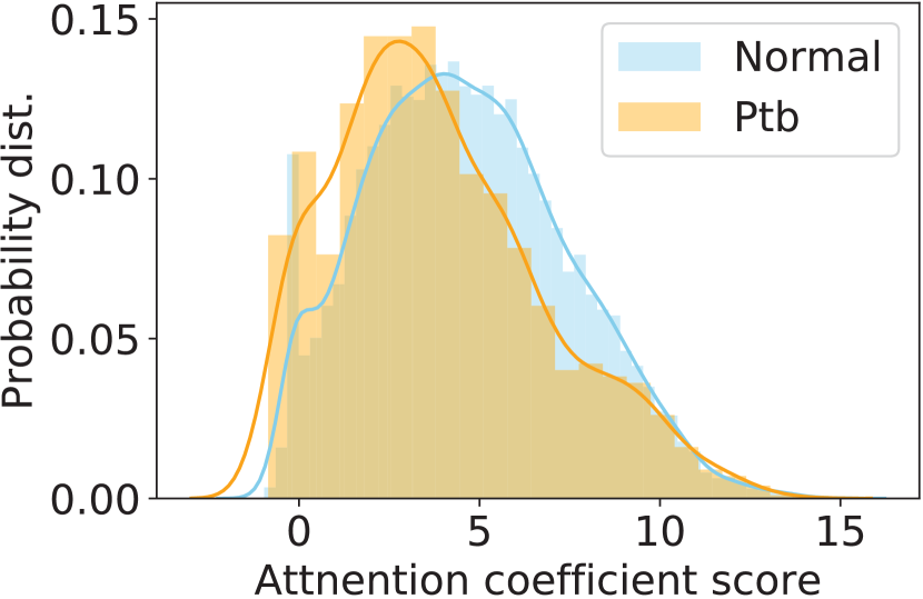
(b) With penalized aggregation.

Figure 3. Distributions of attention coefficients in PA-GNN.

5.3.2. Varying the Meta-Optimization Algorithm.

Next, we study the contribution of the meta-optimization algorithm. As discussed in Section 4.2, three ablations are created accordingly: $\text{{PA-GNN}}_{2nd}$, $\text{{PA-GNN}}_{ft}$, and $\text{{PA-GNN}}_{jt}$. $\text{{PA-GNN}}_{2nd}$ ignores clean graphs and rely on a second-time attack to generate perturbed edges. $\text{{PA-GNN}}_{ft}$ omit the meta-optimization process, training the model initialization on clean graphs and their adversarial counterparts jointly. We then fine-tune the initialization for $\mathcal{G}$ using the classification loss $\mathcal{L}_{c}$. $\text{{PA-GNN}}_{jt}$ further simplifies $\text{{PA-GNN}}_{ft}$ by adding $\mathcal{G}$ to the joint training step. Note that we remove $\mathcal{L}_{dist}$ for $\mathcal{G}$ because detailed perturbation information is unknown for a poisoned graph. All three variants are evaluated on Reddit dataset, and their performance is reported in Table 4.

$\text{{PA-GNN}}_{2nd}$ performs the worst among all variations. Because perturbed edges from the adversarial attack can significantly hurt the accuracy, treating them as clean edges is not a feasible solution. $\text{{PA-GNN}}_{ft}$, and $\text{{PA-GNN}}_{jt}$ slightly out-perform PA-GNN when $\mathcal{G}$ is clean. This is not amazing since more training data can contribute to the model. However, their performance decreases rapidly as the perturbation rate raises up. Because the data distribution of a perturbed graph is changed, barely aggregate all available data is not an optimal solution for defending adversarial attack. It is vital to design PA-GNN which leverages clean graphs from similar domains for improving the robustness of GNNs. At last, $\text{{PA-GNN}}_{np}$ consistently out-performs $\text{{PA-GNN}}_{ft}$, and $\text{{PA-GNN}}_{jt}$ in perturbed cases. shown advantages of the meta-optimization algorithm which utilizes clean graphs to train the model regardless of the penalized aggregation mechanism.

5.4. Parameter Sensitivity Analysis

We investigate the sensitivity of $\eta$ and $\lambda$ for PA-GNN. $\eta$ controls the penalty of perturbed edges, while $\lambda$ balances the classification objective and the penalized aggregation mechanism. Generally, a larger $\eta$ pull the distribution of perturbed edges farther away from that of normal edges. We explore the sensitivity on Pubmed and Reddit datasets, both with a 10% perturbation rate. We alter $\eta$ and $\lambda$ among $\{0,1,10,100,1000\}$ and $\{0,50,100,200,400,800\}$, respectively. The performance of PA-GNN is illustrated in Figure 4. As we can see, the accuracy of PA-GNN is relatively smooth when parameters are within certain ranges. However, extremely large values of $\eta$ and $\lambda$ result in low performances on both datasets, which should be avoided in practice. Moreover, increasing $\lambda$ from 0 to 1 improves the accuracy on both datasets, demonstrating the proposed penalized aggregation mechanism can improve the robustness of PA-GNN.

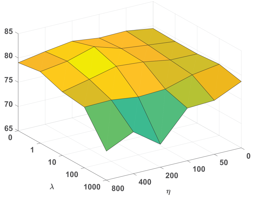
(a) Pubmed with 10% Ptb.

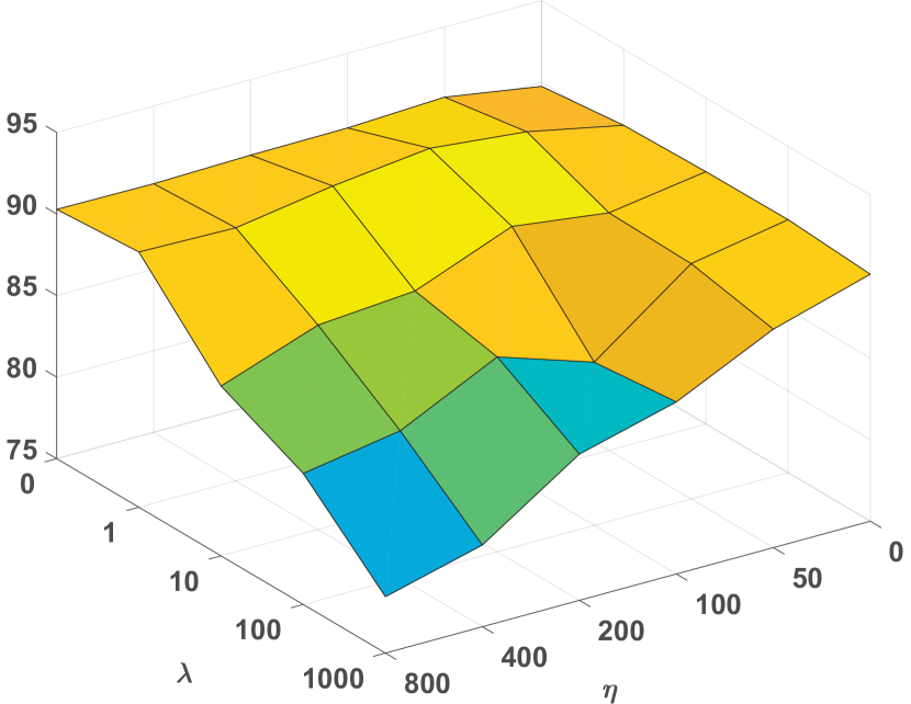
(b) Reddit with 10% Ptb.

Figure 4. Parameter sensitivity analysis.

6. Conclusion and Future Work

In this paper, we study a new problem of exploring extra clean graphs for learning a robust GNN against the poisoning attacks on a target graph. We propose a new framework PA-GNN, that leverages penalized attention mechanism to learn the ability to reduce the negative impact from perturbations on clean graphs and meta-optimization to transfer the alleviation ability to the target poisoned graph. Experimental results of node classification tasks demonstrate the efficacy of PA-GNN against different poisoning attacks. In the future, we would like to explore the potential of transfer learning for improving robustness on other models, such as community detection and graph classification.

- (1)
- Akoglu et al. (2015) Leman Akoglu, Hanghang Tong, and Danai Koutra. 2015. Graph based anomaly detection and description: a survey. Data mining and knowledge discovery 29, 3 (2015), 626–688.
- Bojchevski and Günnemann (2019) Aleksandar Bojchevski and Stephan Günnemann. 2019. Adversarial Attacks on Node Embeddings via Graph Poisoning. In ICML.
- Bruna et al. (2013) Joan Bruna, Wojciech Zaremba, Arthur Szlam, and Yann LeCun. 2013. Spectral networks and locally connected networks on graphs. arXiv preprint arXiv:1312.6203 (2013).
- Chen et al. (2018) Jinyin Chen, Yangyang Wu, Xuanheng Xu, Yixian Chen, Haibin Zheng, and Qi Xuan. 2018. Fast gradient attack on network embedding. arXiv preprint arXiv:1809.02797 (2018).
- Cheng et al. (2018) Minhao Cheng, Thong Le, Pin-Yu Chen, Jinfeng Yi, Huan Zhang, and Cho-Jui Hsieh. 2018. Query-efficient hard-label black-box attack: An optimization-based approach. arXiv preprint arXiv:1807.04457 (2018).
- Dai et al. (2018) Hanjun Dai, Hui Li, Tian Tian, Xin Huang, Lin Wang, Jun Zhu, and Le Song. 2018. Adversarial attack on graph structured data. ICML (2018).
- Defferrard et al. (2016) Michaël Defferrard, Xavier Bresson, and Pierre Vandergheynst. 2016. Convolutional neural networks on graphs with fast localized spectral filtering. In Advances in neural information processing systems. 3844–3852.
- Ding et al. (2019a) Kaize Ding, Jundong Li, Rohit Bhanushali, and Huan Liu. 2019a. Deep Anomaly Detection on Attributed Networks. In SDM.
- Ding et al. (2019b) Kaize Ding, Yichuan Li, Jundong Li, Chenghao Liu, and Huan Liu. 2019b. Graph Neural Networks with High-order Feature Interactions. arXiv preprint arXiv:1908.07110 (2019).
- Fan et al. (2019) Wenqi Fan, Yao Ma, Qing Li, Yuan He, Eric Zhao, Jiliang Tang, and Dawei Yin. 2019. Graph Neural Networks for Social Recommendation. In The World Wide Web Conference. ACM, 417–426.
- Finn et al. (2017) Chelsea Finn, Pieter Abbeel, and Sergey Levine. 2017. Model-agnostic meta-learning for fast adaptation of deep networks. In ICML.
- Gao et al. (2018) Hongyang Gao, Zhengyang Wang, and Shuiwang Ji. 2018. Large-scale learnable graph convolutional networks. In KDD.
- Goodfellow et al. (2014) Ian J Goodfellow, Jonathon Shlens, and Christian Szegedy. 2014. Explaining and harnessing adversarial examples. arXiv preprint arXiv:1412.6572 (2014).
- Hamilton et al. (2017) Will Hamilton, Zhitao Ying, and Jure Leskovec. 2017. Inductive representation learning on large graphs. In NeurIPS.
- Henaff et al. (2015) Mikael Henaff, Joan Bruna, and Yann LeCun. 2015. Deep convolutional networks on graph-structured data. arXiv preprint arXiv:1506.05163 (2015).
- Hochreiter et al. (2001) Sepp Hochreiter, A Steven Younger, and Peter R Conwell. 2001. Learning to learn using gradient descent. In ICANN. Springer, 87–94.
- Huang et al. (2019) Chao Huang, Xian Wu, Xuchao Zhang, Chuxu Zhang, Jiashu Zhao, Dawei Yin, and Nitesh V Chawla. 2019. Online Purchase Prediction via Multi-Scale Modeling of Behavior Dynamics. In KDD. ACM, 2613–2622.
- Jin et al. (2019) Ming Jin, Heng Chang, Wenwu Zhu, and Somayeh Sojoudi. 2019. Power up! Robust Graph Convolutional Network against Evasion Attacks based on Graph Powering. arXiv preprint arXiv:1905.10029 (2019).
- Kipf and Welling (2016) Thomas N Kipf and Max Welling. 2016. Semi-Supervised Classification with Graph Convolutional Networks. arXiv preprint arXiv:1609.02907 (2016).
- Lee et al. (2017) Jaekoo Lee, Hyunjae Kim, Jongsun Lee, and Sungroh Yoon. 2017. Transfer learning for deep learning on graph-structured data. In AAAI.
- Li et al. (2019c) Ruirui Li, Liangda Li, Xian Wu, Yunhong Zhou, and Wei Wang. 2019c. Click Feedback-Aware Query Recommendation Using Adversarial Examples. In The World Wide Web Conference. ACM, 2978–2984.
- Li et al. (2018b) Ruoyu Li, Sheng Wang, Feiyun Zhu, and Junzhou Huang. 2018b. Adaptive graph convolutional neural networks. In AAAI.
- Li et al. (2019a) Yingwei Li, Song Bai, Cihang Xie, Zhenyu Liao, Xiaohui Shen, and Alan L Yuille. 2019a. Regional Homogeneity: Towards Learning Transferable Universal Adversarial Perturbations Against Defenses. arXiv preprint arXiv:1904.00979 (2019).
- Li et al. (2018a) Yingwei Li, Song Bai, Yuyin Zhou, Cihang Xie, Zhishuai Zhang, and Alan Yuille. 2018a. Learning Transferable Adversarial Examples via Ghost Networks. arXiv preprint arXiv:1812.03413 (2018).
- Li et al. (2019b) Yandong Li, Lijun Li, Liqiang Wang, Tong Zhang, and Boqing Gong. 2019b. NATTACK: Learning the Distributions of Adversarial Examples for an Improved Black-Box Attack on Deep Neural Networks. ICML (2019).
- Ma et al. (2019a) Yao Ma, Suhang Wang, Charu C. Aggarwal, and Jiliang Tang. 2019a. Graph Convolutional Networks with EigenPooling. In KDD.
- Ma et al. (2019b) Yao Ma, Suhang Wang, Charu C. Aggarwal, Dawei Yin, and Jiliang Tang. 2019b. Multi-dimensional Graph Convolutional Networks. In SDM.
- Ma et al. (2019c) Yao Ma, Suhang Wang, Lingfei Wu, and Jiliang Tang. 2019c. Attacking Graph Convolutional Networks via Rewiring. arXiv preprint:1906.03750 (2019).
- Monti et al. (2017) Federico Monti, Davide Boscaini, Jonathan Masci, Emanuele Rodola, Jan Svoboda, and Michael M Bronstein. 2017. Geometric deep learning on graphs and manifolds using mixture model cnns. In CVPR.
- Niepert et al. (2016) Mathias Niepert, Mohamed Ahmed, and Konstantin Kutzkov. 2016. Learning convolutional neural networks for graphs. In ICML.
- Pennington et al. (2014) Jeffrey Pennington, Richard Socher, and Christopher Manning. 2014. Glove: Global vectors for word representation. In EMNLP.
- Santoro et al. (2016) Adam Santoro, Sergey Bartunov, Matthew Botvinick, Daan Wierstra, and Timothy Lillicrap. 2016. Meta-learning with memory-augmented neural networks. In ICML.
- Sen et al. (2008) Prithviraj Sen, Galileo Namata, Mustafa Bilgic, Lise Getoor, Brian Galligher, and Tina Eliassi-Rad. 2008. Collective classification in network data. AI magazine 29, 3 (2008), 93–93.
- Shu et al. (2018) Kai Shu, Suhang Wang, Jiliang Tang, Yilin Wang, and Huan Liu. 2018. Crossfire: Cross media joint friend and item recommendations. In WSDM.
- Sun et al. (2019) Yiwei Sun, Suhang Wang, Xianfeng Tang, Tsung-Yu Hsieh, and Vasant Honavar. 2019. Node Injection Attacks on Graphs via Reinforcement Learning. arXiv preprint arXiv:1909.06543 (2019).
- Vaswani et al. (2017) Ashish Vaswani, Noam Shazeer, Niki Parmar, Jakob Uszkoreit, Llion Jones, Aidan N Gomez, Lukasz Kaiser, and Illia Polosukhin. 2017. Attention is all you need. In Advances in neural information processing systems. 5998–6008.
- Veličković et al. (2017) Petar Veličković, Guillem Cucurull, Arantxa Casanova, Adriana Romero, Pietro Lio, and Yoshua Bengio. 2017. Graph attention networks. arXiv preprint arXiv:1710.10903 (2017).
- Vinyals et al. (2016) Oriol Vinyals, Charles Blundell, Timothy Lillicrap, Daan Wierstra, et al. 2016. Matching networks for one shot learning. In Advances in neural information processing systems. 3630–3638.
- Wu et al. (2019c) Felix Wu, Tianyi Zhang, Amauri Holanda de Souza Jr, Christopher Fifty, Tao Yu, and Kilian Q Weinberger. 2019c. Simplifying graph convolutional networks. arXiv preprint arXiv:1902.07153 (2019).
- Wu et al. (2019b) Huijun Wu, Chen Wang, Yuriy Tyshetskiy, Andrew Docherty, Kai Lu, and Liming Zhu. 2019b. Adversarial Examples on Graph Data: Deep Insights into Attack and Defense. In IJCAI.
- Wu et al. (2019a) Zonghan Wu, Shirui Pan, Fengwen Chen, Guodong Long, Chengqi Zhang, and Philip S Yu. 2019a. A comprehensive survey on graph neural networks. arXiv preprint arXiv:1901.00596 (2019).
- Xu et al. (2019b) Han Xu, Yao Ma, Haochen Liu, Debayan Deb, Hui Liu, Jiliang Tang, and Anil Jain. 2019b. Adversarial attacks and defenses in images, graphs and text: A review. arXiv preprint arXiv:1909.08072 (2019).
- Xu et al. (2019a) Kaidi Xu, Hongge Chen, Sijia Liu, Pin-Yu Chen, Tsui-Wei Weng, Mingyi Hong, and Xue Lin. 2019a. Topology Attack and Defense for Graph Neural Networks: An Optimization Perspective. arXiv preprint arXiv:1906.04214 (2019).
- Yao et al. (2019a) Huaxiu Yao, Yiding Liu, Ying Wei, Xianfeng Tang, and Zhenhui Li. 2019a. Learning from Multiple Cities: A Meta-Learning Approach for Spatial-Temporal Prediction. In The World Wide Web Conference. ACM, 2181–2191.
- Yao et al. (2019b) Huaxiu Yao, Ying Wei, Junzhou Huang, and Zhenhui Li. 2019b. Hierarchically Structured Meta-learning. In ICML. 7045–7054.
- Yao et al. (2019c) Huaxiu Yao, Chuxu Zhang, Ying Wei, Meng Jiang, Suhang Wang, Junzhou Huang, Nitesh V Chawla, and Zhenhui Li. 2019c. Graph Few-shot Learning via Knowledge Transfer. arXiv preprint arXiv:1910.03053 (2019).
- Zhang et al. (2018) Jiani Zhang, Xingjian Shi, Junyuan Xie, Hao Ma, Irwin King, and Dit-Yan Yeung. 2018. Gaan: Gated attention networks for learning on large and spatiotemporal graphs. arXiv preprint arXiv:1803.07294 (2018).
- Zhu et al. (2019) Dingyuan Zhu, Ziwei Zhang, Peng Cui, and Wenwu Zhu. 2019. Robust Graph Convolutional Networks Against Adversarial Attacks. In KDD.
- Zügner et al. (2018) Daniel Zügner, Amir Akbarnejad, and Stephan Günnemann. 2018. Adversarial attacks on neural networks for graph data. In KDD.
- Zügner and Günnemann (2019) Daniel Zügner and Stephan Günnemann. 2019. Certifiable robustness and robust training for graph convolutional networks. In KDD.
- Zügner and Günnemann (2019) Daniel Zügner and Stephan Günnemann. 2019. Adversarial Attacks on Graph Neural Networks via Meta Learning. In ICLR.