Modeling UV Radiation Feedback from Massive Stars:
III. Escape of Radiation from Star-forming Giant Molecular Clouds

Abstract

Using a suite of radiation hydrodynamic simulations of star cluster formation in turbulent clouds, we study the escape fraction of ionizing (Lyman continuum) and non-ionizing (FUV) radiation for a wide range of cloud masses and sizes. The escape fraction increases as H II regions evolve and reaches unity within a few dynamical times. The cumulative escape fraction before the onset of the first supernova explosion is in the range 0.05–0.58; this is lower for higher initial cloud surface density, and higher for less massive and more compact clouds due to rapid destruction. Once H II regions break out of their local environment, both ionizing and non-ionizing photons escape from clouds through fully ionized, low-density sightlines. Consequently, dust becomes the dominant absorber of ionizing radiation at late times and the escape fraction of non-ionizing radiation is only slightly larger than that of ionizing radiation. The escape fraction is determined primarily by the mean $\langle\tau\rangle$ and width $\sigma$ of the optical-depth distribution in the large-scale cloud, increasing for smaller $\langle\tau\rangle$ and/or larger $\sigma$. The escape fraction exceeds (sometimes by three orders of magnitude) the naive estimate $e^{-\langle\tau\rangle}$ due to non-zero $\sigma$ induced by turbulence. We present two simple methods to estimate, within $\sim 20\%$, the escape fraction of non-ionizing radiation using the observed dust optical depth in clouds projected on the plane of sky. We discuss implications of our results for observations, including inference of star formation rates in individual molecular clouds, and accounting for diffuse ionized gas on galactic scales.

1 Introduction

Intense ultraviolet (UV) radiation produced by massive OB stars regulates heating, ionization, and chemistry in the interstellar medium (ISM), both within and beyond star-forming clouds. Lyman continuum (LyC) photons capable of ionizing hydrogen (with energy $h\nu>13.6{\,{\rm eV}}$) create H II regions around massive stars or clusters in giant molecular clouds (GMCs). Due to elevated local pressure, H II regions dynamically expand and strongly affect GMC evolution and star formation within them (McKee & Ostriker, 2007; Krumholz et al., 2014; Dale, 2015; Krumholz et al., 2018, and references therein). Far-UV (FUV) photons (with energy $6.0{\,{\rm eV}}<h\nu<13.6{\,{\rm eV}}$) can penetrate deep into GMCs to ionize and dissociate numerous atomic and molecular species, forming photodissociation regions. Emission lines from these photodissociation regions are crucial probes of the physical conditions in star-forming GMCs (Hollenbach & Tielens, 1999).

Some fraction of UV photons emitted by massive stars can escape from GMCs without being absorbed by gas and dust. The leakage of ionizing photons from “classical” H II regions embedded in GMCs is the most likely source of photoionization of warm ionized gas in the diffuse ISM (the diffuse ionized gas (DIG) or warm ionized medium (WIM); e.g., Reynolds, 1984; Haffner et al., 2009). The further escape of stellar ionizing photons from galaxies into the intergalactic medium is crucial to the reionization history of the early universe (e.g., Loeb & Barkana, 2001; Robertson et al., 2010; Bromm & Yoshida, 2011; Wise, 2019). It is estimated that an escape fraction of least 10–30% is required for typical stellar populations in star-forming galaxies to induce significant reionization at a redshift $7\lesssim z\lesssim 9$ (e.g., Bouwens et al. 2011; Finkelstein et al. 2012; Robertson et al. 2015, but see Finkelstein et al. 2019), placing demanding requirements on the cloud-scale escape fraction.

Equally important to the escape of ionizing photons, FUV photons escaping into the diffuse ISM determine the strength of the interstellar background radiation field (Parravano et al., 2003). Via the photoelectric effect on dust, this FUV radiation provides the dominant form of heating for the diffuse atomic ISM (e.g Wolfire et al., 1995, 2003), amounting to most of the gas mass in galaxies. Diffuse FUV heating controls the thermal pressure in the diffuse ISM ($P_{\rm th}\propto J_{\rm FUV}$), providing partial support against gravity and contributing to the self-regulation of star formation on galactic scales (e.g., Ostriker et al., 2010; Kim et al., 2013).

Despite the importance of escaping LyC and FUV radiation from star-forming regions, direct observational constraints on the escape fraction from GMCs have been scarce and remain uncertain (e.g., Smith & Brooks, 2007; Doran et al., 2013; Voges et al., 2008; Pellegrini et al., 2012; Binder & Povich, 2018; McLeod et al., 2019). Smith & Brooks (2007) estimated the escape fraction of ionizing radiation, $f_{\rm esc,i}$, from the Carina Nebula, using spectral classifications of individual massive stars to establish the baseline for the total ionizing photon production rate (Smith, 2006). By comparing to the observed free-free emission, they estimated that $\sim 25\%$ of ionizing photons escape through holes in the nebula. They also estimated the escape fraction of non-ionizing radiation, $f_{\rm esc,n}\sim 20\%$, by comparing the total FUV output of known OB stars with the infrared (IR) emission from the cool dust component. Doran et al. (2013) took a similar approach to estimate $f_{\rm esc,i}\sim 6\%$ for the 30 Doradus region. Voges et al. (2008) compared the observed (extinction-corrected) H$\alpha$ luminosity of H II regions in the Large Magellanic Cloud with the expected H$\alpha$ luminosity from the observed stellar content, finding that $\sim 20$–$30\%$ of H II regions are density-bounded. Pellegrini et al. (2012) investigated $f_{\rm esc,i}$ of individual H II regions in the Large and Small Magellanic Clouds based on the optical depth of H II regions from the map of emission-line ratios such as [S II]/[O III]. They found the luminosity-weighted escape fractions amount to $\sim 0.4$, dominated by the most luminous H II regions.

An additional but more indirect constraint on $f_{\rm esc,i}$ is obtained by measuring the contribution of diffuse H$\alpha$ emission relative to the total (diffuse + classical H II regions) H$\alpha$ emission in external galaxies. Provided that photons from massive stars in young clusters dominate in ionizing the diffuse gas and that the galaxy-scale escape fraction is low, the diffuse H$\alpha$ fraction probes the (globally averaged) cloud-scale escape fraction. Deep H$\alpha$ images of nearby galaxies show significant ($\sim 20$–$60\%$) diffuse emission across their disks (e.g., Ferguson et al., 1996; Hoopes et al., 1996; Zurita et al., 2000; Oey et al., 2007; Kreckel et al., 2016; Lacerda et al., 2018; Poetrodjojo et al., 2019). For a sample of 109 H I-selected nearby galaxies, Oey et al. (2007) found that the mean fraction of diffuse H$\alpha$ emission is $0.59$, with a systematically lower diffuse fraction in starburst galaxies. Weilbacher et al. (2018) found that 60% of the H$\alpha$ emission comes from the diffuse ionized gas in the central regions of the interacting Antennae galaxy. Weilbacher et al. (2018) also estimated $f_{\rm esc,i}$ of individual H II regions by comparing their H$\alpha$ luminosity with the LyC production rate estimated from the catalog of young star clusters inside H II regions, and found that the overall cloud-scale escape fraction is consistent with the diffuse fraction.

For a complete accounting, it is necessary to allow for dust absorption of ionizing radiation, and the H$\alpha$ emission must be extinction-corrected, for both star-forming regions and diffuse gas. These adjustments can be quite important, and “raw” H$\alpha$ fractions may be misleading subject to the relative roles of dust in the diffuse and dense ISM. For example, the relative probability of losing LyC photons to ionization vs. dust absorption depends inversely on the ionization parameter (e.g., Dopita et al., 2003), which is higher in H II regions than the diffuse ISM; H$\alpha$ from dense star forming regions is strongly extincted compared to H$\alpha$ from the diffuse ISM.

While there are some (albeit uncertain) empirical estimates regarding escape fractions of photons from star forming regions, on the theory side current understanding is more limited. Theoretical models of the internal structure of H II regions are mostly limited to spherical, ionization-bounded H II regions with $f_{\rm esc,i}=0$ (e.g., Petrosian et al., 1972; Inoue, 2002; Dopita et al., 2003; Draine, 2011), so they are not useful for studying escape fractions (but see Rahner et al., 2017). Massive stars form in clusters deeply embedded within dense cores of GMCs (Tan et al., 2014), so that nascent H II regions are highly compact and ionization bounded (Hoare et al., 2007). However, expansion with evolution leads to a situation where H II regions become density bounded and exhibit extended envelopes (e.g., Kim & Koo, 2001, 2003), since turbulence and stellar feedback create low-density, optically-thin holes through which radiation can escape. As the processes involved are highly nonlinear, time dependent, and lacking in any simplifying symmetry, radiation hydrodynamic (RHD) simulations are essential for quantifying photon escape fractions.

In recent years, several numerical studies have investigated the UV escape fraction on cloud scales using simulations of star cluster formation with self-consistent radiation feedback (Dale et al., 2012, 2013; Walch et al., 2012; Howard et al., 2017; Raskutti et al., 2017; Kimm et al., 2019). For instance, Dale et al. (2012, 2013) performed simulations of cloud disruption with the effects of photoionization feedback included. Using cloud models with the initial virial parameter of $\alpha_{\rm vir,0}=1.4$ or $4.6$, they found that $f_{\rm esc,i}$ increases with time as clouds are dispersed by feedback. For clouds with low escape velocities and large virial ratios, $f_{\rm esc,i}$ reaches $\gtrsim 50\%$ before the onset of first supernovae ($3\,{\rm Myr}$ after massive star formation). Howard et al. (2017, 2018) simulated cluster formation in an initially unbound GMCs with $\alpha_{\rm vir,0}=3$ and masses $10^{4}$–$10^{6}\,M_{\odot}$ under the influence of both photoionization and radiation pressure feedback. They studied the temporal changes of $f_{\rm esc,i}$ in these models during the first $\sim 5\,{\rm Myr}$ of the cloud evolution after massive star formation. They found that $f_{\rm esc,i}$ is highly variable with time because the surrounding gas is highly turbulent, and that the highest escape fraction ($f_{\rm esc,i}>0.9$) is achieved only in intermediate cloud masses ($\sim 5\times 10^{4}\,M_{\odot}$). More recently, Kimm et al. (2019) performed RHD simulations of cloud destruction by the combined action of photoionization, radiation pressure, and supernovae explosions, also following evolution of several chemical species. They found a strong positive relationship between the star formation efficiency and the time-averaged LyC escape fraction, as stronger feedback clears away the gas and lowers the neutral gas covering fraction more rapidly.

Although the previous numerical studies mentioned above have greatly improved our understanding of the cloud-scale escape fraction, they are not without limitations. One limitation has been in the radiation model and cloud parameter space. For example, the simulations of Dale et al. (2012, 2013) did not incorporate the effects of dust absorption on $f_{\rm esc,i}$. Howard et al. (2017, 2018) considered clouds with fixed mean density, so that they covered only a narrow range of the parameter space. Kimm et al. (2019) mostly focused on two basic cloud models while considering low and high SFE and low and high metallicity. In addition, most of these previous studies focused only on $f_{\rm esc,i}$, but did not study $f_{\rm esc,n}$, which is crucial for understanding emission from star-forming clouds as well as the interstellar radiation field. Raskutti et al. (2017), on the other hand, studied the escape of non-ionization radiation, but did not include ionizing photons.

In a series of numerical RHD studies, we have been investigating star cluster formation in turbulent GMCs with diverse properties, as well as the impact of stellar radiation feedback on cloud disruption. In Kim et al. (2017, hereafter Paper I), we presented the implementation and tests of our numerical RHD method, which adopts the adaptive ray-tracing algorithm of Abel & Wandelt (2002) for point source radiative transfer. In Kim et al. (2018, hereafter Paper II), we presented results from models with a range of GMC size and mass, assessing the dependence of star formation efficiency (SFE) and cloud lifetime on the cloud surface density, quantifying mass loss due to photoevaporation, and analyzing momentum injection and disruption driven by gas and radiation pressure forces.

In this paper, we reanalyze the simulations presented in Paper II, focusing on the escape fractions of both ionizing and non-ionizing radiation. Our main objectives are as follows. First, we explore how $f_{\rm esc,i}$ and $f_{\rm esc,n}$ from star-forming GMCs vary with time and calculate the cumulative escape fractions before the epoch of the first supernova. Second, we compare the fraction of ionizing radiation absorbed by gas and dust with the prediction from analytic solutions for static, spherical, ionization-bounded H II regions. Third, we investigate how closely $f_{\rm esc,i}$ is related to $f_{\rm esc,n}$. Fourth, we investigate how escape fractions can be estimated from the angular distribution of the optical depth seen from the sources. Lastly, we propose methods to estimate the escape fractions from the mean optical depth or the area distribution of the optical depth projected along the line of sight of an external observer.

The rest of this paper is organized as follows. In Section 2, we briefly describe our numerical methods and initial conditions of the simulations. In Section 3, we present results on the overall evolution of the simulated clouds. This includes quantifying the fractions of photons that are absorbed by gas, by dust, and that escape from the clouds. In Section 4, we calculate optical depth distributions as seen from the luminosity center or by an external observer, and we relate these distributions to the measured escape fractions. In Section 5, we summarize and discuss our main results. In Appendix A, we develop and apply a subgrid model to explore how radiation absorbed in the immediate vicinity of sources (which we do not numerically resolve) may affect SFE estimates. In Appendix B, we explore the potential effect of dust destruction in ionized gas on the escape fraction of radiation.

2 Numerical Methods

We study the escape fractions of ionizing and non-ionizing radiation from star-forming, turbulent GMCs based on a suite of RHD simulations presented in Paper II. These simulations were performed using the grid-based magnetohydrodynamics code Athena (Stone et al., 2008), equipped with modules for self-gravity, sink particles, and point source radiative transfer. In this section, we briefly summarize the numerical methods and cloud models. The reader is referred to Paper I and Paper II for technical details as well as more quantitative results.

2.1 Radiation Hydrodynamics Scheme

We solve the equations of hydrodynamics in conservation form using the van Leer type time integrator (Stone & Gardiner, 2009), HLLC Riemann solver, and piecewise linear spatial reconstruction method. We employ the sink particle method of Gong & Ostriker (2013) to handle cluster formation and ensuing mass accretion. A Lagrangian sink particle (representing a subcluster of young stars) is created if a gas cell (1) has the density above a threshold value set by the Larson-Penston self-gravitating collapse solution imposed at the grid scale, (2) has a converging velocity field around it, and (3) is at the local minimum of the gravitational potential. The gas mass that is accreted onto a sink particle is calculated based on the fluxes returned by the Riemann solver at the boundary faces of a $3^{3}$-cell control volume surrounding it. The gravitational potential from gas and stars is computed using the fast Fourier transform Poisson solver with the vacuum boundary conditions (Skinner & Ostriker, 2015).

The UV radiative output of a star cluster is calculated based on the mass-luminosity relation obtained from Monte-Carlo simulations for the spectra of a zero-age main sequence population with a Chabrier initial mass function (IMF) (Kim et al., 2016). For a given total cluster mass $M_{*,{\rm tot}}$, we compute the total UV luminosity $L=L_{\rm i}+L_{\rm n}\equiv\Psi M_{*,{\rm tot}}$ and the total ionizing photon rate $Q_{\rm i}=L_{\rm i}/(h\nu_{\rm i})\equiv\Xi M_{*,{\rm tot}}$, where $L_{\rm i}$ and $L_{\rm n}$ refer to the luminosity of ionizing and non-ionizing radiation, respectively, and $h\nu_{\rm i}=18{\,{\rm eV}}$ is the mean energy of ionizing photons. The light-to-mass ratios $\Psi$ and $\Xi$ are in general functions of $M_{*,{\rm tot}}$. To allow for the effects of incomplete sampling of the IMF at the high-mass end, we fit $\Psi$ and $\Xi$ to the median values of multiple realizations of the IMF. It turns out that $\Psi\rightarrow 912\,L_{\odot}\,M_{\odot}^{-1}$ and $\Xi\rightarrow 5.05\times 10^{46}\,{\rm s}^{-1}\,M_{\odot}^{-1}$ in the limit of a fully sampled IMF ($M_{*,{\rm tot}}\gtrsim 10^{4}\,M_{\odot}$), while they sharply decline with decreasing $M_{*,{\rm tot}}\lesssim 10^{3}\,M_{\odot}$. We treat the instantaneous set of star particles as a single cluster to determine the total luminosity, and the luminosity of each sink particle is assigned in proportion to its mass. We do not consider temporal evolution of $\Psi$ and $\Xi$ in the present work.

We adopt the adaptive ray-tracing method (Abel & Wandelt, 2002) to track the radiation field emitted from multiple sources. Photon packets injected at the position of each source particle propagate along the rays whose directions are determined by the HEALPix scheme of Górski et al. (2005), which divides the unit sphere into equal-area pixels. Rays are split adaptively to ensure that each cell is crossed by at least four rays per source. The length of a line segment passing through the cell is used to calculate the optical depth that is required to evaluate the volume-averaged radiation energy densities $\mathcal{E}_{\rm i},\mathcal{E}_{\rm n}$ and fluxes $\mathbf{F}_{\rm i},\mathbf{F}_{\rm n}$ in the ionizing and non-ionizing frequency bins at every cell.

As sources of UV opacity, we consider absorption of ionizing photons by neutral hydrogen and that of both ionizing and non-ionizing photons by dust. We adopt constant values of $\sigma_{\rm ph}=6.3\times 10^{-18}\,{\rm cm}^{2}\,{\rm H}^{-1}$ for the photoionization cross section (Krumholz et al., 2007) and $\sigma_{\rm d,i/n}=\sigma_{\rm d}=1.17\times 10^{-21}\,{\rm cm}^{2}\,{\rm H}^{-1}$ for the dust absorption cross section per hydrogen (or cross section per unit gas mass $\kappa_{\rm d}=\sigma_{\rm d}/\mu_{\rm H}=500\,{\rm cm}^{2}\,\,{\rm g}^{-1}$, with $\mu_{\rm H}=1.4m_{\rm H}$ being the mean molecular weight) (Draine, 2011). We discuss the potential impact of dust destruction in ionized regions on the escape fraction in Section 5.2.4. The resulting radiation energy and flux densities are used to calculate the local photoionization rate $\mathcal{I}=n_{\rm H^{0}}\sigma_{\rm ph}c\mathcal{E}_{\rm i}/(h\nu_{\rm i})$ and radiation pressure force $\frac{n_{{\rm H^{0}}}\sigma_{\rm ph}}{c}\mathbf{F}_{\rm i}+\frac{n_{\rm H}\sigma_{\rm d}}{c}(\mathbf{F}_{\rm i}+\mathbf{F}_{\rm n})$ on dusty gas, where $n_{\rm H}$ and $n_{\rm H^{0}}$ are the number density of total and neutral hydrogen, respectively.

We solve the continuity equation for neutral hydrogen including source and sink terms due to recombination and photoionization, adopting case B recombination rate coefficient $\alpha_{\rm B}=3.03\times 10^{-13}\,{\rm cm}^{3}\,{\rm s}^{-1}(T/8000\,{\rm K})^{-0.7}$ (Krumholz et al., 2007). The source and sink terms are explicitly updated every substep in an operator split fashion. The gas temperature is set to vary smoothly as a function of the neutral gas fraction between $20\,{\rm K}$ and $8000\,{\rm K}$, corresponding to the temperature of fully neutral and fully ionized gas, respectively. The use of constant equilibrium temperature is a good approximation if the gas cooling time is short compared to the dynamical timescale (e.g., Lefloch & Lazareff, 1994). Although our model cannot represent the detailed thermal structure of H II regions because we neglect ionization of helium and do not follow specific heating/cooling processes, it still captures the essential physics needed to follow the dynamics of H II regions with self-consistent star formation, which is crucial for modeling escape of radiation.

2.2 Initial and Boundary Conditions

We establish initial conditions of our model clouds following Skinner & Ostriker (2015). We start with a uniform-density gas sphere with mass $M_{\rm 0}$ and radius $R_{\rm 0}$ placed at the center of a computational box, surrounded by a tenuous medium with density $10^{3}$ times lower than the cloud. The box is a cube with each side $L_{\rm box}=4R_{\rm 0}$. Our standard resolution is $N=256$ cells in one direction, although we also run simulations with $N=128$ or $512$ to test convergence for the fiducial model. Initially, the cloud is completely neutral and seeded by a (decaying) turbulent velocity field with a power spectrum $|\delta\mathbf{v}_{k}|^{2}\propto k^{-4}$ over the wavenumber range $k\in\left[2,64\right]\times 2\pi/L_{\rm box}$. The initial cloud is set to be marginally bound, with the initial virial parameter $\alpha_{\rm vir,0}\equiv 5\sigma_{v,0}^{2}R_{\rm 0}/(3GM_{\rm 0})=2$, where $\sigma_{v,0}$ is the turbulent velocity dispersion (e.g., Bertoldi & McKee, 1992).

We adopt strict outflow (diode-like) boundary conditions both at the outer boundaries of the computational domain and at the boundary faces of the control volume surrounding each sink particle. The $3^{3}$ control-volume cells serve as internal ghost zones within the simulation domain. Because of the presence of a point mass which is also a source of radiation, gravity and hydrodynamic variables are unresolved within control volumes, and we do not attempt to model photon-gas interactions. Instead, we simply allow all of the photons emitted by a sink particle to emerge from the control volume without absorption, corresponding to $f_{\rm esc,*}=1$, where $f_{\rm esc,*}$ denotes the escape fraction of radiation from the control volume (i.e., “subgrid” scale). In reality, photon-gas interactions inside the control volume would lower $f_{\rm esc,*}$ below unity and thus reduce the overall efficiency of radiation feedback on cloud scales. In Appendix A, we explore the effect of varying $f_{\rm esc,*}$ on the cloud-scale SFE, using simulations with only non-ionizing radiation. There, we discuss the plausible range of $f_{\rm esc,*}$, and show that the final stellar mass in our fiducial cloud is increased only modestly ($\sim 0.1M_{\rm 0}$) if $f_{\rm esc,*}$ is allowed to drop below unity.

Table 1: Model parameters and simulation results

Model	$M_{0}$	$R_{0}$	$\Sigma_{0}$	$n_{\rm H,0}$	$t_{\rm ff,0}$	$t_{\rm dest}$	$Q_{\rm i,max}$	$f_{\rm esc,i}^{\rm cum}$	$f_{\rm phot,i}^{\rm cum}$	$f_{\rm dust,i}^{\rm cum}$	$f_{\rm esc,n}^{\rm cum}$	$f_{\rm dust,n}^{\rm cum}$
(1)	(2)	(3)	(4)	(5)	(6)	(7)	(8)	(9)	(10)	(11)	(12)	(13)
M1E5R50	$10^{5}$	$50.0$	$12.7$	$5.5$	$18.5$	$10.4$	$10^{50.2}$	$0.58$	$0.28$	$0.14$	$0.72$	$0.28$
M1E5R40	$10^{5}$	$40.0$	$19.9$	$10.8$	$13.2$	$10.4$	$10^{50.4}$	$0.48$	$0.34$	$0.18$	$0.61$	$0.39$
M1E5R30	$10^{5}$	$30.0$	$35.4$	$25.5$	$8.6$	$8.2$	$10^{50.6}$	$0.45$	$0.36$	$0.20$	$0.56$	$0.44$
M1E4R08	$10^{4}$	$8.0$	$49.7$	$134.7$	$3.7$	$3.9$	$10^{49.0}$	$0.47$	$0.38$	$0.15$	$0.58$	$0.42$
M1E6R80	$10^{6}$	$80.0$	$49.7$	$13.5$	$11.8$	$8.2$	$10^{51.7}$	$0.12$	$0.56$	$0.33$	$0.23$	$0.77$
M5E4R15	$5\times 10^{4}$	$15.0$	$70.7$	$102.2$	$4.3$	$6.3$	$10^{50.5}$	$0.37$	$0.39$	$0.24$	$0.46$	$0.54$
M1E5R20	$\bf 10^{5}$	$\bf 20.0$	$\bf 79.6$	$\bf 86.2$	$\bf 4.7$	$\bf 6.5$	$10^{50.8}$	$\bf 0.30$	$\bf 0.38$	$\bf 0.32$	$\bf 0.39$	$\bf 0.61$
M1E4R05	$10^{4}$	$5.0$	$127.3$	$551.8$	$1.9$	$3.8$	$10^{49.7}$	$0.35$	$0.40$	$0.26$	$0.42$	$0.58$
M1E6R45	$10^{6}$	$45.0$	$157.2$	$75.7$	$5.0$	$6.9$	$10^{52.0}$	$0.10$	$0.54$	$0.36$	$0.14$	$0.86$
M1E5R10	$10^{5}$	$10.0$	$318.3$	$689.7$	$1.7$	$3.7$	$10^{51.1}$	$0.12$	$0.50$	$0.38$	$0.16$	$0.84$
M1E4R03	$10^{4}$	$3.0$	$353.7$	$2554.6$	$0.9$	$2.7$	$10^{49.9}$	$0.49$	$0.28$	$0.23$	$0.52$	$0.48$
M1E6R25	$10^{6}$	$25.0$	$509.3$	$441.4$	$2.1$	$5.0$	$10^{52.3}$	$0.05$	$0.62$	$0.32$	$0.07$	$0.93$
M1E4R02	$10^{4}$	$2.0$	$795.8$	$8621.6$	$0.5$	$1.9$	$10^{50.3}$	$0.45$	$0.38$	$0.17$	$0.47$	$0.53$
M1E5R05	$10^{5}$	$5.0$	$1273.2$	$5517.8$	$0.6$	$2.1$	$10^{51.4}$	$0.38$	$0.38$	$0.24$	$0.39$	$0.61$
M1E5R20_N128	$10^{5}$	$20.0$	$79.6$	$86.2$	$4.7$	$5.3$	$10^{50.9}$	$0.25$	$0.40$	$0.35$	$0.35$	$0.65$
M1E5R20_N512	$10^{5}$	$20.0$	$79.6$	$86.2$	$4.7$	$7.2$	$10^{50.8}$	$0.28$	$0.44$	$0.28$	$0.36$	$0.64$

Note. — Column 1: model name indicating initial cloud mass and radius. Column 2: initial gas mass ($M_{\odot}$). Column 3: initial radius (${\rm pc}$). Column 4: initial gas surface density ($M_{\odot}\,{\rm pc}^{-2}$). Column 5: initial number density of H (${\rm cm}^{-3}$). Column 6: initial free-fall time (${\rm Myr}$). Column 7: cloud destruction timescale (${\rm Myr}$). Column 8: maximum ionizing photon production rate (${\rm s}^{-1}$). Column 9: cumulative escape fraction of ionizing photons at $t_{*,0}+3\,{\rm Myr}$. Column 10: cumulative hydrogen absorption fraction of ionizing photons at $t_{*,0}+3\,{\rm Myr}$. Column 11: cumulative dust absorption fraction of ionizing photons at $t_{*,0}+3\,{\rm Myr}$. Column 12: cumulative dust absorption fraction of non-ionizing photons at $t_{*,0}+3\,{\rm Myr}$. The fiducial model M1E5R20 is shown in bold.

2.3 Cloud Model

We consider 14 models that span two orders of magnitude in mass ($10^{4}\,M_{\odot}<M_{\rm 0}<10^{6}\,M_{\odot}$) and surface density ($12.7\,M_{\odot}\,{\rm pc^{-2}}<\Sigma_{\rm 0}<1.27\times 10^{3}\,M_{\odot}\,{\rm pc^{-2}}$) to explore a range of star-forming environments. For example, low surface density ($\Sigma_{\rm 0}\sim 10^{2}\,M_{\odot}\,{\rm pc^{-2}}$) and massive ($M_{\rm 0}\sim 10^{5}$–$10^{6}\,M_{\odot}$) clouds are representative of typical GMCs in the Milky Way and normal spiral galaxies, whereas high surface density ($\Sigma_{\rm 0}\gtrsim 500\,M_{\odot}\,{\rm pc^{-2}}$) and low mass ($M_{\rm 0}\lesssim 10^{5}\,M_{\odot}$) clouds correspond to individual cluster-forming clumps within GMCs (e.g., Tan et al., 2014). The Columns 1–6 of Table 1 respectively list the model names, mass $M_{\rm 0}$, radius $R_{\rm 0}$, surface density $\Sigma_{\rm 0}=M_{\rm 0}/(\pi R_{\rm 0}^{2})$, number density of hydrogen $n_{\rm H,0}$, and free-fall time $t_{\rm ff,0}=\tfrac{\pi}{2}\sqrt{R_{\rm 0}^{3}/(2GM_{\rm 0})}$ of the initial model clouds. Given the initial virial parameter $\alpha_{\rm vir,0}=2$ in all our simulations, the initial turbulent Mach number varies from $\mathcal{M}_{0}=\sigma_{v,0}/c_{\rm s}=$ 6 to 33 for the sound speed of neutral gas $c_{\rm s}=0.26\,{\rm km}\,{\rm s}^{-1}$. We take the “Orion-like” model M1E5R20 with $M_{\rm 0}=10^{5}\,M_{\odot}$ and $R_{\rm 0}=20\,{\rm pc}$ as our fiducial case. Models M1E5R20_N128 and M1E5R20_N512 correspond to the fiducial cloud at different resolution with $N=128$ and 512, respectively.

2.4 Absorption and Escape Fractions of Radiation

The escape of ionizing radiation is hindered by absorption by dust and neutral hydrogen. Let $Q_{\rm gas,i}=\int\mathcal{I}dV$ denote the total photoionization rate and $Q_{\rm dust,i}=\int n_{\rm H}\sigma_{\rm d}c\mathcal{E}_{\rm i}/(h\nu_{\rm i})dV$ the total dust absorption rate. Then, the rate of ionizing photons escaping from the computational domain is given by $Q_{\rm esc,i}=Q_{\rm i}-Q_{\rm gas,i}-Q_{\rm dust,i}$. The adaptive ray tracing calculates $\mathcal{E}_{\rm i}$ at every cell and keeps track of $Q_{\rm esc,i}$ explicitly, allowing us to calculate the hydrogen absorption fraction, dust absorption fraction, and escape fraction defined as

$$f_{\rm gas,i} \equiv\frac{Q_{\rm gas,i}}{Q_{\rm i}},$$ (1)

$$f_{\rm dust,i} \equiv\frac{Q_{\rm dust,i}}{Q_{\rm i}},$$ (2)

$$f_{\rm esc,i} \equiv\frac{Q_{\rm esc,i}}{Q_{\rm i}}=1-f_{\rm gas,i}-f_{\rm dust,i},$$ (3)

respectively. These instantaneous quantities are luminosity-weighted averages over individual sources. We also calculate the cumulative escape fraction defined as

$$f_{\rm esc,i}^{\rm cum}(t^{\prime})\equiv\dfrac{\int_{t_{*,0}}^{t}Q_{\rm i,esc}\,dt}{\int_{t_{*,0}}^{t}Q_{\rm i}\,dt},$$ (4)

and similarly for the cumulative absorption fractions, $f_{\rm gas,i}^{\rm cum}$ and $f_{\rm dust,i}^{\rm cum}$. Here, $t_{*,0}$ is the time at which the first sink particle is created and radiative feedback is turned on, and $t^{\prime}=t-t_{*,0}$. We similarly monitor the dust absorption fraction $f_{\rm dust,n}$ and the escape fraction $f_{\rm esc,n}=1-f_{\rm dust,n}$ of non-ionizing photons.

3 Time Evolution

Figure 1: Snapshots of the fiducial model M1E5R20 ($M_{\rm 0}=10^{5}\,M_{\odot}$ and $R_{\rm 0}=20\,{\rm pc}$) at $0.5$, $1.5$, $3.0$, and $5.0\,{\rm Myr}$ (left to right) after the first star formation. (top row) Gas surface density projected along the $y$-direction. In each panel, the projected positions of star particles are indicated by small circles, with age indicated by color. The star particle center of mass is indicated with a star symbol. The plus signs and the dotted circles mark the center of mass and the half-mass radius of the gas in projection, respectively. (middle row) Slices through the most massive star particle (marked with $\times$ symbol) of the number density of neutral (blue) and ionized (orange) hydrogen in the $x$–$z$ plane. Only the star particles within $\Delta y=\pm R_{\rm 0}/2$ of the slice are shown. (bottom row) Hammer projection maps of the angular distributions of the escape probabilities $\exp(-\tau^{\rm c}_{\rm i})$ and $\exp(-\tau^{\rm c}_{\rm n})$ for ionizing and non-ionizing radiation as seen from the position of the most massive sink particle. At the times shown (left to right), the instantaneous escape fraction is $f_{\rm esc,i}=(15,31,37,59)\%$ for ionizing radiation and $f_{\rm esc,n}=(31,39,45,65)\%$ for non-ionizing radiation.

Figure 2: Same as Figure 1 but for model M1E5R05 with $M_{\rm 0}=10^{5}\,M_{\odot}$ and $R_{\rm 0}=5\,{\rm pc}$ at times $t^{\prime}=$ $0.3$, $1.0$, $2.0$, and $2.5\,{\rm Myr}$ after the first star formation. From left to right, the instantaneous escape fraction radiation is $f_{\rm esc,i}=(2.3,3.1,26,88)\%$ for ionizing radiation and $f_{\rm esc,n}=(3.8,4.5,28,88)\%$ for non-ionizing radiation.

Figure 3: Evolution of the instantaneous escape fraction $f_{\rm esc,i}$ (top), the hydrogen absorption fraction $f_{\rm gas,i}$ (middle), and the dust absorption fraction $f_{\rm dust,i}$ (bottom) for ionizing radiation. Time is measured from the creation of the first star particle ($t^{\prime}=t-t_{*,0}$), in units of $t_{\rm ff,0}$ (left) or Myr (right). All models are shown, with the thickness and color of each line indicating the initial cloud mass $M_{\rm 0}$ and surface density $\Sigma_{\rm 0}$, respectively. With small $t_{\rm ff,0}$, high-$\Sigma_{\rm 0}$ clouds evolve rapidly: most gas is cleared away and $f_{\rm esc,i}$ reaches unity in a few Myr, before massive stars explode as supernovae.

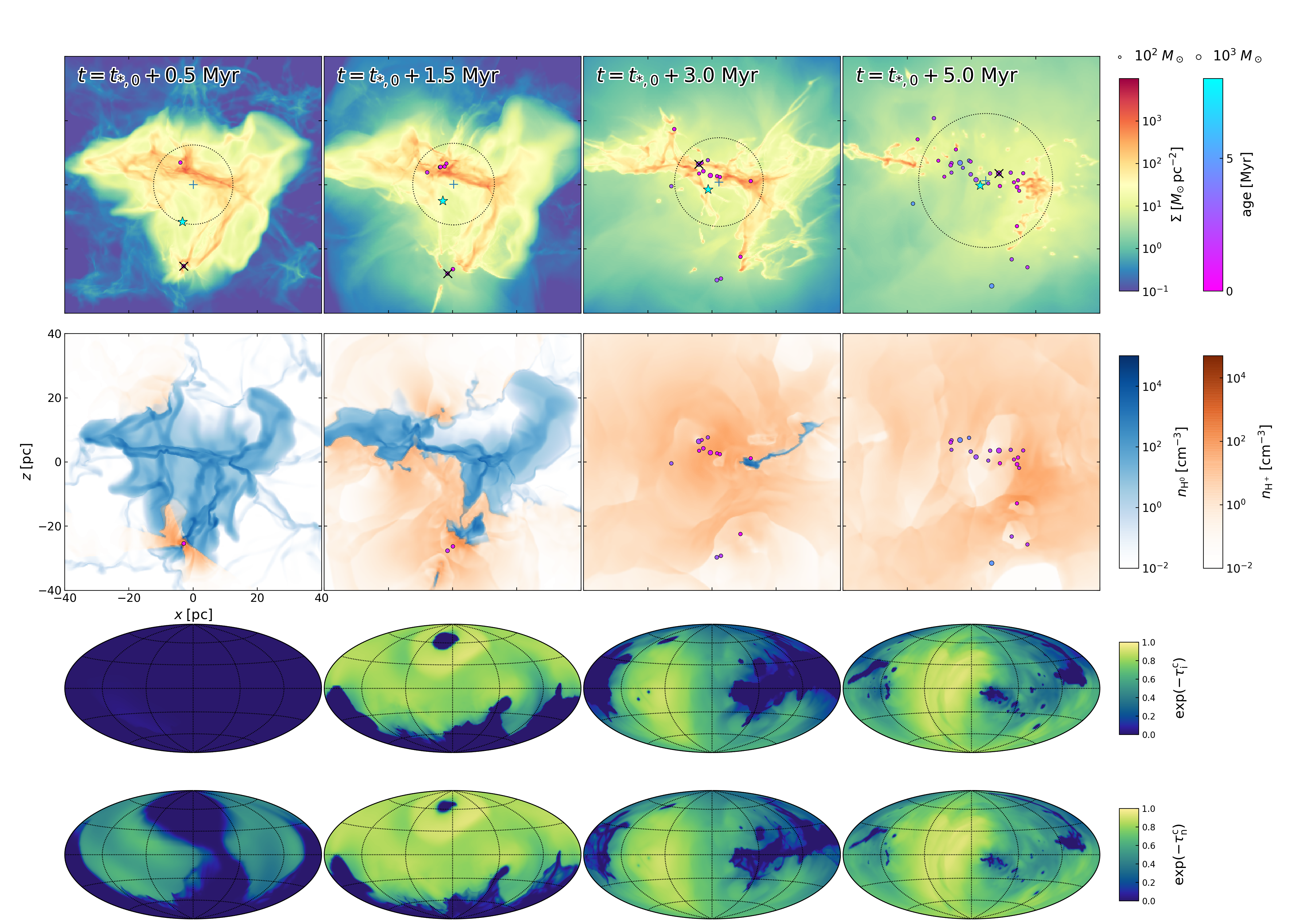
We begin by presenting temporal evolution of our fiducial model, with a focus on the absorption and escape fractions of radiation. Figure 1 displays snapshots of the fiducial model ($M_{\rm 0}=10^{5}\,M_{\odot}$ and $R_{\rm 0}=20\,{\rm pc}$, with $\Sigma_{\rm 0}=80\,M_{\odot}\,{\rm pc^{-2}}$ and $n_{\rm H,0}=86\,{\rm cm}^{-3}$) at times $t^{\prime}=0.5$, $1.5$, $3$, and $5\,{\rm Myr}$, from left to right, after the first star formation event occurring at $t_{*,0}=1.87\,{\rm Myr}$. From top to bottom, the rows show gas surface density projected along the $y$-axis, slices of the neutral (blue) and ionized (orange) gas density through the most massive sink particle in the $x$–$z$ plane, and the Hammer projections of the angular distributions of the escape probabilities, $\exp(-\tau^{\rm c}_{\rm i})$ and $\exp(-\tau^{\rm c}_{\rm n})$, of the ionizing and non-ionizing radiation, respectively, as seen from the most massive sink particle. Here, the superscripts “c” indicate the optical depth calculated outward from a point within the cloud to the edge of the simulation domain. In the top row, the dotted circles draw the projected regions enclosing half the total gas mass in the simulation domain, while the star symbols mark the projected center of mass of the star particles represented by small circles in the top and second rows.

Cloud evolution is initially driven by supersonic turbulence that readily produces shock-compressed filaments and clumps. The densest parts of these structures become gravitationally unstable and soon spawn sink particles. Ensuing radiation feedback from the sink particles form small H II regions around them. The H II regions expand outward and break out of the natal clumps, eventually merging with each other. In this process, the low density gas becomes rather quickly ionized by the passage of R-type ionization fronts, increasing its volume fraction from 27% at $t^{\prime}=0.2\,{\rm Myr}$ to 78% at $t^{\prime}=1.5\,{\rm Myr}$ in the fiducial model. The gas that acquires sufficient radial momentum via thermal and radiation pressures leaves the simulation domain, which in turn destroys the cloud and limits the SFE. We measure the cloud destruction timescale as the time taken to photoevaporate and/or eject 95% of the initial cloud mass after the onset of radiation feedback (so that only 5% of the initial cloud mass is left over as the neutral phase in the simulation domain), i.e., $t_{\rm dest}\equiv t_{{\rm neu},5\%}-t_{*,0}$, and the net SFE as the fraction of the initial cloud mass that turned into stars over the cloud lifetime, i.e., $\varepsilon_{*}\equiv M_{*,{\rm final}}/M_{\rm 0}$. For the fiducial model, we find $t_{\rm dest}=6.5\,{\rm Myr}=1.39t_{\rm ff,0}$ and $\varepsilon_{*}\equiv M_{*,{\rm final}}/M_{\rm 0}=0.13$. As discussed in Paper II, the dominant feedback mechanism is photoionization rather than radiation pressure: 81% of the initial cloud mass is lost by photoevaporation; the radial momentum injected by thermal pressure in this model is $\sim 5$ times higher than that from radiation pressure.

As the Hammer projections in Figure 1 show, an appreciable fraction of radiation can escape from the H II regions even before the complete destruction of the natal clumps. For instance, the instantaneous escape fractions amount to $f_{\rm esc,i}=15\%$ and $f_{\rm esc,n}=31\%$ at $t^{\prime}=0.5\,{\rm Myr}$ when about $98\%$ of the gas mass is in the neutral phase. This is because turbulence naturally creates sightlines with low optical depth along which the H II regions are density bounded, permitting easy escape of radiation. As star formation continues and gas photoevaporates, the fraction of solid angle with optically thick, ionization-bounded sightlines steadily decreases. This lowers the hydrogen absorption fraction, while increasing the escape fraction more or less monotonically with time (see Figure 2 of Paper II). The dust absorption fraction reaches $f_{\rm dust,i}\sim 37\%$ at $t^{\prime}=1\,{\rm Myr}$ and is then maintained at $\sim 30$–$35\%$ for about $3.5\,{\rm Myr}$ before starting to decline gradually.

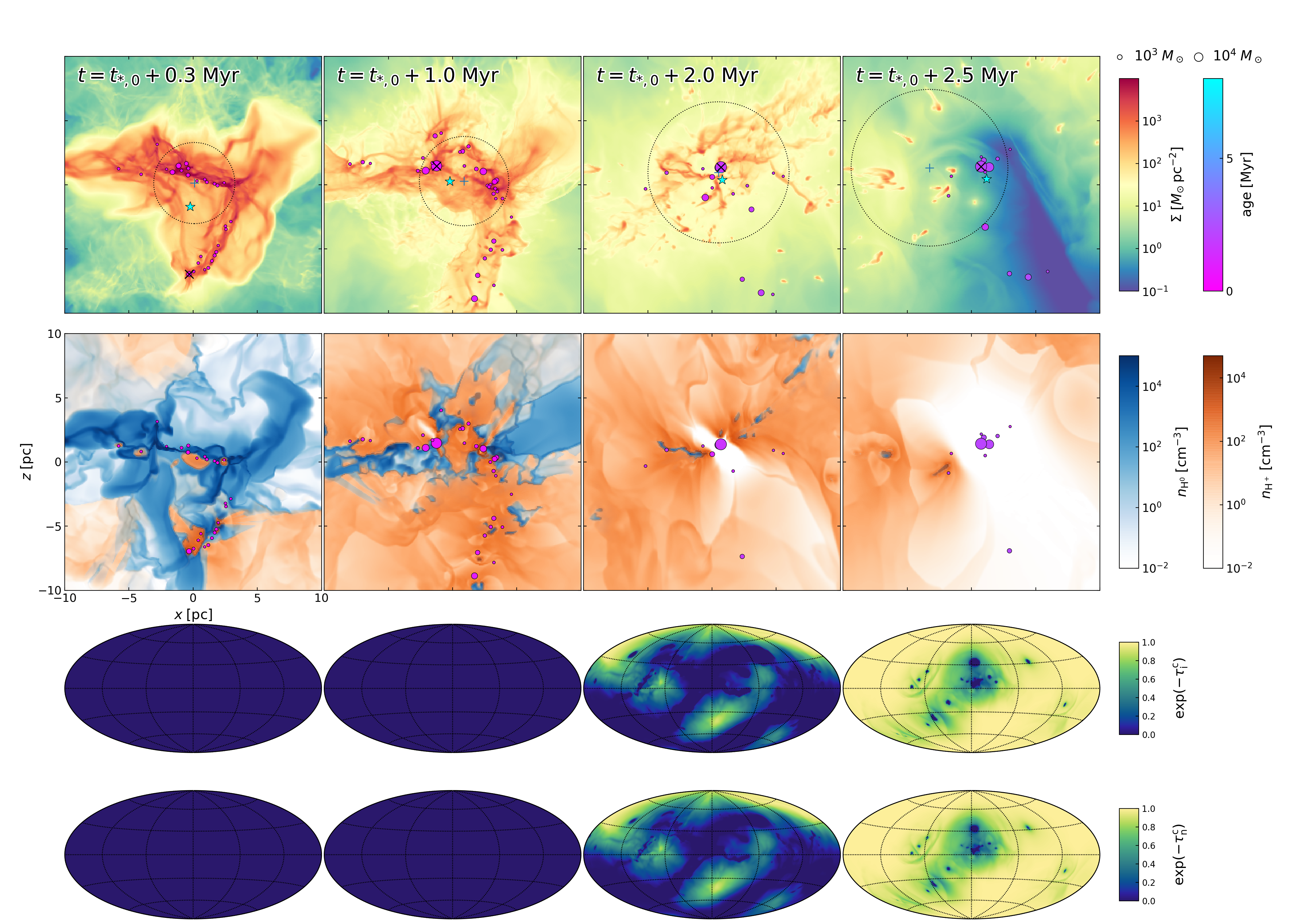
While the overall dynamical evolution of other models is qualitatively similar, we find that the evolution of the absorption and escape fractions depend on the initial surface density. Figure 2 plots snapshots of gas surface density, slices of neutral and ionized volume density, and angular distributions of the radiation escape probabilities for model M1E5R05 ($M_{\rm 0}=10^{5}M_{\rm 0},R_{\rm 0}=5\,{\rm pc}$, $\Sigma_{\rm 0}=1.3\times 10^{3}\,M_{\odot}\,{\rm pc^{-2}}$, and $n_{0}=5.5\times 10^{3}\rm\,{\rm cm}^{-3}$). Compared to the fiducial run with $\Sigma_{\rm 0}=80\,M_{\odot}\,{\rm pc^{-2}}$, the denser recombination layers and deeper gravitational potential in model M1E5R05 make radiation feedback less effective in photoevaporating the neutral gas and ejecting gas by radiation and thermal pressures, yielding a higher SFE of $\varepsilon_{*}=0.51$ (Paper II; see also Geen et al. 2017; Grudić et al. 2018). The cloud destruction time is only $t_{\rm dest}=2.1\,{\rm Myr}$ since all dynamical processes are rapid at high density; the free-fall time for this model is just $t_{\rm ff,0}=0.6\,{\rm Myr}$. Due to high dust column, trapped H II regions barely break out and both $f_{\rm esc,i}$ and $f_{\rm esc,n}$ remain very small during most of the cloud evolution, as evidenced by the angular distributions of the escape probabilities shown in Figure 2. For example, at $t^{\prime}=1.0\,{\rm Myr}$, $f_{\rm esc,i}=0.02$ even though the ionized gas fills $\sim 80\%$ of the entire volume. At $t^{\prime}=2\,{\rm Myr}$ when star formation is completed and the ionized-gas volume filling factor is 97%, $f_{\rm esc,i}$ and $f_{\rm esc,n}$ increase only to 0.26 and 0.28, respectively. The cumulative escape and absorption fractions at $t^{\prime}=2\,{\rm Myr}$ are $f_{\rm esc,i}^{\rm cum}=0.08$, $f_{\rm gas,i}^{\rm cum}=0.63$, $f_{\rm dust,i}^{\rm cum}=0.29$, $f_{\rm esc,n}^{\rm cum}=0.10$, and $f_{\rm dust,n}^{\rm cum}=0.90$ in this model.

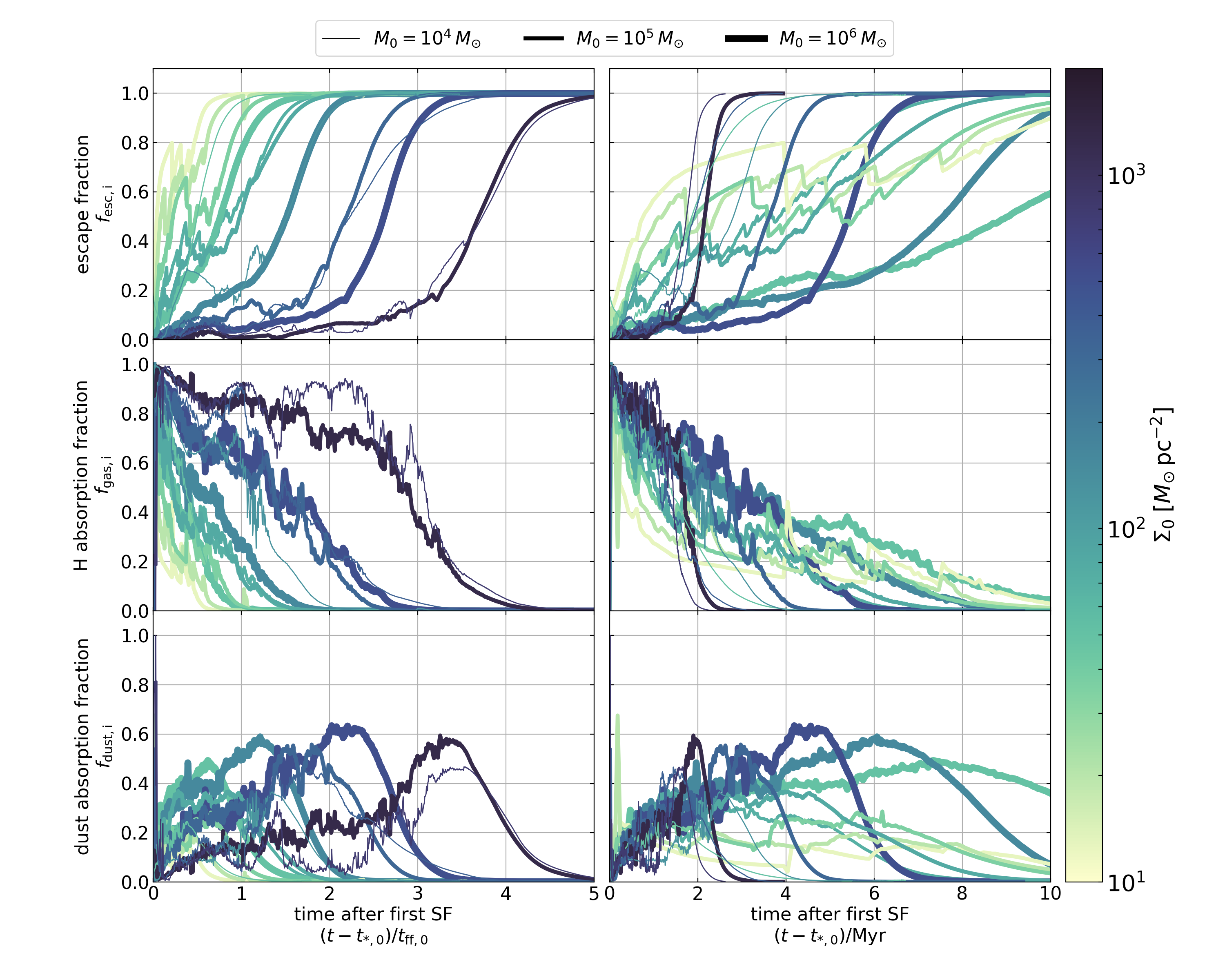
Figure 3 plots the ionizing radiation history of $f_{\rm esc,i}$ (top), $f_{\rm gas,i}$ (middle), and $f_{\rm dust,i}$ (bottom) as functions of the time for all models. The line thickness and color indicate $M_{\rm 0}$ and $\Sigma_{\rm 0}$, respectively. For all models, time is measured since the first star formation, and shown in units of $t_{\rm ff,0}$ and Myr in the left and right panels, respectively. Overall, $f_{\rm esc,i}$ increases as H II regions evolve, consistent with expectations and with results from previous simulations (Walch et al., 2012; Dale et al., 2013; Kimm et al., 2019). The escape of ionizing radiation is limited primarily by photoionization in early evolutionary stages and by dust absorption in late stages. The dust absorption fraction peaks slightly before cloud destruction, and vanishes as the remaining gas is cleared out. Although higher-$\Sigma_{\rm 0}$ clouds appear to live longer in terms of $t_{\rm ff,0}$, they are actually destroyed earlier in real time. Note that clouds with $\Sigma_{\rm 0}\gtrsim 300\,M_{\odot}\,{\rm pc^{-2}}$ and $M_{\rm 0}\leq 10^{5}\,M_{\odot}$ (M1E4R03, M1E4R02, M1E5R05) are destroyed in less than $3\,{\rm Myr}$ after the onset of star formation (Column 7 in Table 1), resulting in substantial escape of radiation before the advent of supernova explosions (Section 3.3).

3.1 Comparison with Spherical Models

Figure 4: Dependence of (a) the instantaneous escape fraction $f_{\rm esc,i}$, (b) the hydrogen absorption fraction $f_{\rm gas,i}$, and (c) the dust absorption fraction $f_{\rm dust,i}$ of ionizing radiation on the product of the total photoionization rate $Q_{\rm gas,i}$ and the rms number density of the ionized gas $n_{\rm i,rms}$. The thickness and color of each line indicate the initial gas mass $M_{\rm 0}$ and surface density $\Sigma_{\rm 0}$ in the model. The orange dashed and solid lines in (b) and (c) draw the predictions of the theoretical models for embedded ($f_{\rm esc,i}=0$), spherical, static H II regions with (Draine, 2011) and without (Petrosian et al., 1972) the effects of radiation pressure, respectively. The open symbols in (b) are the observational estimates for $f_{\rm gas,i}$ from the Galactic H II regions by Inoue et al. (2001, diamonds), Inoue (2002, squares), and Binder & Povich (2018, circles).

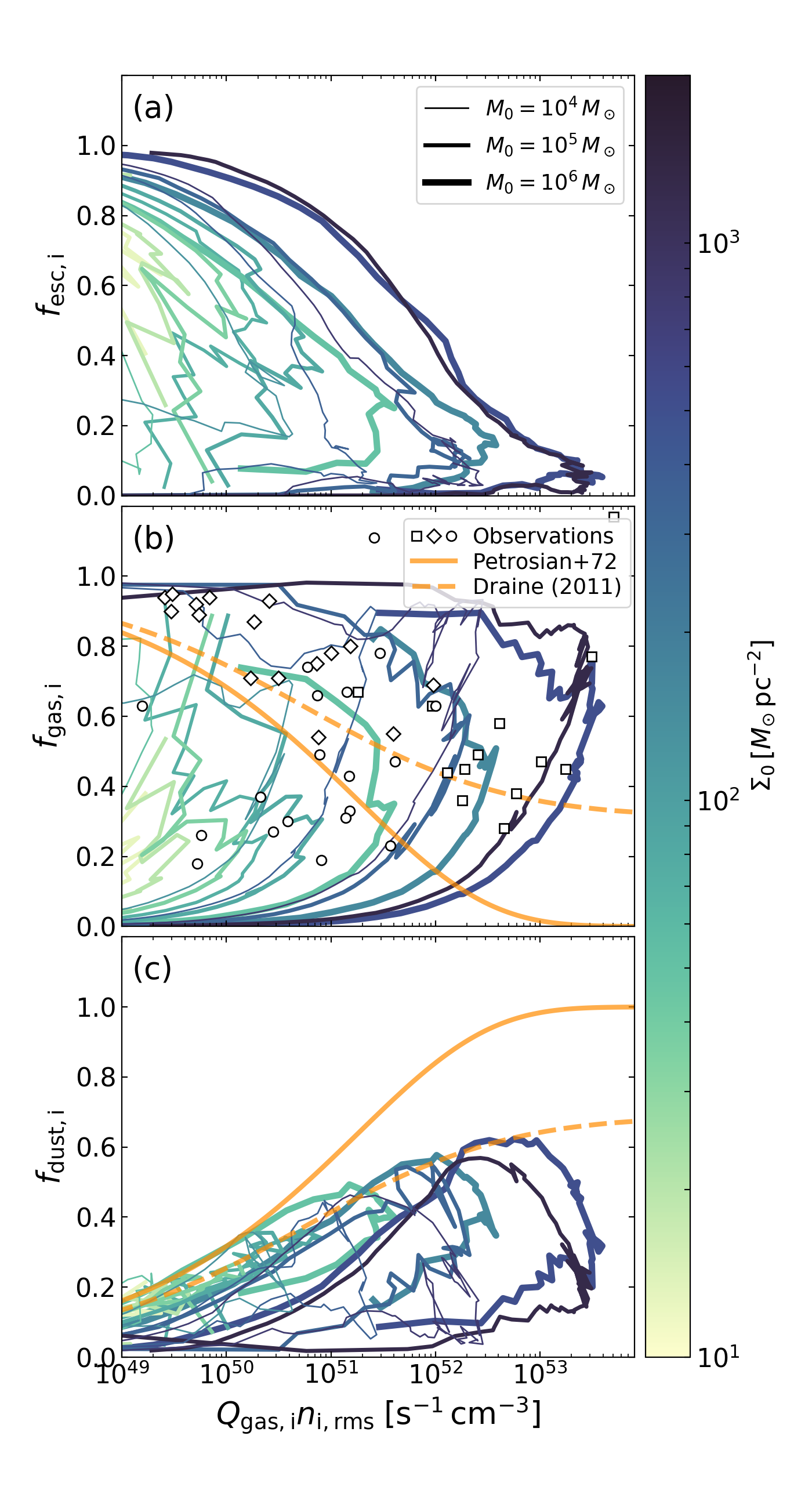
It is interesting to compare the hydrogen and dust absorption fractions calculated in our simulations with the analytic predictions for static, spherical, ionization-bounded ($f_{\rm esc,i}=0$) H II regions. For this purpose, Figure 4 plots as various lines (a) the escape fraction ($f_{\rm esc,i}$), (b) the hydrogen absorption fraction ($f_{\rm gas,i}$), and (c) the dust absorption fraction ($f_{\rm dust,i}$) of ionizing radiation for all models. The abscissa is the product of the effective ionizing photon rate $Q_{\rm gas,i}=f_{\rm gas,i}Q_{\rm i}$ and the rms number density of the ionized gas $n_{\rm i,rms}=(\int_{\rm\mathcal{V}}n_{\rm i}^{2}dV/\int_{\rm\mathcal{V}}dV)^{1/2}$, which are often accessible to observers via free-free radio continuum and/or nebular emission lines. We take the integration volume $\mathcal{V}$ as a sphere around the cluster center that encloses 99% of $\int n_{\rm i}^{2}dV$ over the whole domain. In each model, $Q_{\rm gas,i}n_{\rm i,rms}$ increases with time in the early phase of evolution, but decreases as gas is removed by feedback in the late phase. Thus, individual model tracks start at the left, evolve to the right, and then return toward the left. Meanwhile, $f_{\rm esc,i}$ tends to secularly increase and $f_{\rm gas,i}$ to decrease with time, while $f_{\rm dust,i}$ starts small, reaches a maximum, and then decreases again.

Petrosian et al. (1972) derived an analytic expression for the dust absorption fraction for a uniform-density, embedded, spherical H II region with a constant dust-to-gas ratio (see also Inoue, 2002). Their predictions for $f_{\rm gas,i}$ and $f_{\rm dust,i}$ ($=1-f_{\rm gas,i}$ since $f_{\rm esc,i}\equiv 0$), both as functions of $Q_{\rm gas,i}n_{\rm i,rms}$, are plotted as orange solid lines in Figure 4(b) and (c). This model predicts that the photon absorption is dominated by dust when $Q_{\rm gas,i}n_{\rm i,rms}$ is very large. Also considering a spherical H II region but including radiation pressure on dust and solving for the dynamical equilibrium radial profiles, Draine (2011) found that strong radiation pressure acting on dusty gas creates a central cavity and an outer high-density shell. The resulting absorption fractions are plotted as dashed lines in Figure 4. Because of the enhanced density in the outer radiation-compressed shell in the Draine (2011) model, recombination raises the neutral fraction and hydrogen can absorb a larger fraction of ionizing photons, raising $f_{\rm gas,i}$ and lowering $f_{\rm dust,i}$ relative to the uniform model of Petrosian et al. (1972). In the limit of $Q_{\rm i}n_{\rm i,rms}\rightarrow\infty$, the Draine (2011) model predicts $f_{\rm gas,i}\rightarrow 0.31$ and $f_{\rm dust,i}\rightarrow 0.69$ for the parameters we adopt ($\beta=1.41$, $\gamma=7.58$; see Eqs. (6) and (7) in Kim et al. 2016). Although the Draine (2011) solutions were calculated under the assumption of static equilibrium, we previously showed (Kim et al., 2016) that the interior structure of spherical H II regions that are undergoing pressure-driven expansion (with both radiation and gas pressure) are in good agreement with the profiles predicted by Draine (2011). For fixed $Q_{\rm i}$, $n_{\rm i,rms}$ decreases over time; following the Draine (2011) solution for a spherical, embedded H II region, this would correspond to a decrease in $f_{\rm dust,i}$ and increase in $f_{\rm gas,i}$ over time.

Our numerical results show that both $f_{\rm gas,i}$ and $f_{\rm dust,i}$ depend on the evolutionary state and generally do not follow the trends expected for spherical H II regions. This is of course because (1) H II regions in our simulations have highly non-uniform, non-spherical distributions of gas and dust and (2) a significant fraction of photons can escape without being caught by the dusty gas. Even in the embedded phase with $f_{\rm esc,i}\ll 1$, H II regions in high-$\Sigma_{\rm 0}$ clouds have $f_{\rm gas,i}$ higher than the theoretical predictions for given $Q_{\rm gas,i}n_{\rm i,rms}$. This is likely caused by turbulent mixing that transports neutral gas to the interiors of H II regions, making them non-steady and out of ionization-recombination equilibrium. We also note that in a system containing multiple sources with similar individual values of $n_{\rm i,rms}$, $f_{\rm gas,i}$, and $f_{\rm dust,i}$, the numerical curves would appear to the right of the analytic curves because the total $Q_{\rm gas,i}$ would be a multiple of the individual values. However, this cannot account for the orders of magnitude shift to the right relative to the single-source analytic $f_{\rm gas,i}$ curve. Moreover, whereas $f_{\rm gas,i}$ would increase in time for an expanding spherical H II region, in fact $f_{\rm gas,i}$ decreases in time for the simulations (because of escaping radiation).

Although the spherical analytic predictions for $f_{\rm gas,i}$ appear uncorrelated with results from simulations, there is some resemblance between the analytic prediction and the numerical results for $f_{\rm dust,i}$, in that the former marks the upper envelope of the latter’s distribution. One possible reason that this may not be entirely a coincidence is that $f_{\rm dust,i}$ is greatest at a late stage when the H II region most resembles an idealized shell-bounded Strömgren sphere with a central source.

The hydrogen absorption fraction $f_{\rm gas,i}$ of Galactic H II regions has been estimated by Inoue et al. (2001), Inoue (2002), and Binder & Povich (2018). Inoue et al. (2001) estimated $f_{\rm gas,i}$ of Galactic H II regions using the model of Petrosian et al. (1972) for dusty H II regions. For Galctic ultracompact and compact H II regions, Inoue (2002) derived a relation between $f_{\rm gas,i}$ and the ratio between the total IR and unobscured H$\alpha$ (or free-free) fluxes assuming that UV photons absorbed by dust grains are re-emitted in IR. Binder & Povich (2018) estimated $f_{\rm gas,i}$ of massive star forming regions by taking the ratio between the ionizing photon rate obtained from the Planck free-free emission and the total ionizing photon rate estimated from known massive stellar content. Their estimated values of $f_{\rm gas,i}$ are plotted as open diamonds (Inoue et al., 2001), squares (Inoue, 2002), and circles Binder & Povich (2018) in Figure 4(b). We note that Inoue et al. (2001) and Inoue (2002) did not account for radiation escape, so that the observed $f_{\rm gas,i}$ corresponds to an upper limit on the real hydrogen absorption fraction. Draine (2011) attributed the range of observed $f_{\rm gas,i}$ to the variations in the dust-to-gas ratio. Since $f_{\rm gas,i}$ varies during evolution of a star-forming GMC in our simulations, the observed diversity of $f_{\rm gas,i}$ may also reflect that the observed H II regions are at a different evolutionary stage.

3.2 Similarity between $f_{\rm esc,n}$ and $f_{\rm esc,i}$

Figure 5: Evolution of the instantaneous escape fraction of ionizing ($f_{\rm esc,i}$, orange) and non-ionizing ($f_{\rm esc,n}$, blue) radiation for selected models whose mass and radius are specified in each panel. The dotted and dashed lines in black draw the escape fraction of ionizing radiation $\langle\exp(-\tau^{\rm c}_{\rm i})\rangle_{\Omega}$ and non-ionizing radiation $\langle\exp(-\tau^{\rm c}_{\rm n})\rangle_{\Omega}$, respectively, measured from the center of the stellar luminosity (see Section 4.1).

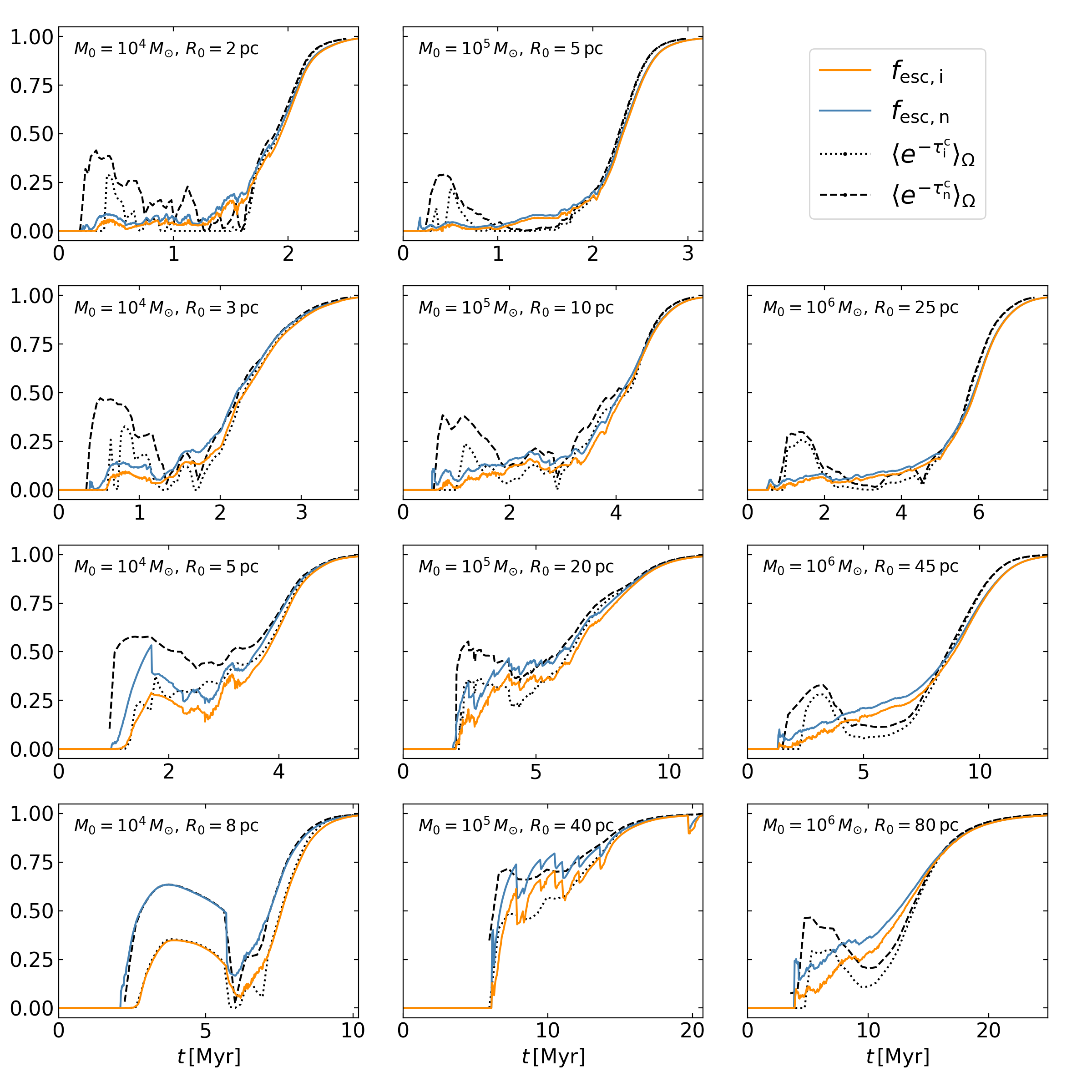
Figure 5 plots evolution of the escape fraction of ionizing (orange) and non-ionizing (blue) radiation for selected models. Notably, the difference between $f_{\rm esc,i}$ and $f_{\rm esc,n}$ is small or only modest. This is also clear from the comparison of the angular distributions of $\exp(-\tau^{\rm c}_{\rm i})$ and $\exp(-\tau^{\rm c}_{\rm n})$, shown in the bottom row of Figures 1 and 2. Although the covering fraction of optically thick clumps/filaments to ionizing radiation is slightly enhanced relative to the non-ionizing counterpart owing to the presence of the recombining gas in photoevaporation flows, overall they appear quite similar. The reason that $f_{\rm esc,n}$ and $f_{\rm esc,i}$ appear so similar is that both ionizing and non-ionizing photons escape through low-density channels in which the gas is almost fully ionized and the H II region is density bounded.

For our models, the difference between the escape probabilities for a single line of sight is $e^{-\tau_{\rm n}}-e^{-\tau_{\rm i}}=e^{-\tau_{\rm n}}(1-e^{-\tau_{\rm ph}})$, where $\tau_{\rm n}=\tau_{\rm d}=\int n_{\rm H}\sigma_{\rm d}d\ell$ is the dust optical depth (assumed to be the same for FUV and EUV) and $\tau_{\rm ph}=\int n_{\rm H^{0}}\sigma_{\rm ph}d\ell=\langle x_{\rm n}\rangle\tfrac{\sigma_{\rm ph}}{\sigma_{\rm d}}\tau_{\rm n}$ is the optical depth due to photoionization of neutral hydrogen, for the mean neutral fraction $\langle x_{\rm n}\rangle$. Note that the difference is bounded above by $e^{-\tau_{\rm n}}$, and also bounded above by $\tau_{\rm ph}$. Both of these upper limits can help to explain why $f_{\rm esc,n}$ and $f_{\rm esc,i}$ are similar, in different circumstances.

If an H II region is ionization bounded ($e^{-\tau_{\rm ph}}\ll 1$) along most sightlines (high covering fraction of neutral gas), the difference between the escape fractions of ionizing and non-ionizing radiation is determined by the dust optical depth. In this case, the escape fractions of ionizing and non-ionizing radiation are small and almost equal as long as $\tau_{\rm d}\gg 1$ along most sightlines. This explains why $f_{\rm esc,n}$ and $f_{\rm esc,i}$ are nearly identical in the highest-$\Sigma_{\rm 0}$ clouds at early times (models M1E4R02, M1E5R05, and M1E6R25). However, in low-$\Sigma_{\rm 0}$ clouds at early times, a non-negligible fraction of non-ionizing photons can escape through sightlines along which the H II region is ionization-bounded ($\tau_{\rm ph}\gg 1$) but has $\tau_{\rm d}\lesssim 1$. This can explain noticeable differences between $f_{\rm esc,i}$ and $f_{\rm esc,n}$ at early times in low-$\Sigma_{\rm 0}$ clouds (models M1E4R08, M1E4R05, M1E5R20, M1E5R40, and M1E6R80).

At late stages of evolution for all models, the H II region breaks out and becomes density bounded along most sightlines (high covering fraction of ionized gas), i.e. $\tau_{\rm ph}\lesssim 1$. In this circumstance, since $e^{-\tau_{\rm n}}-e^{-\tau_{\rm i}}<\tau_{\rm ph}$, the difference between $f_{\rm esc,n}$ and $f_{\rm esc,i}$ will depend on the value of $\tau_{\rm ph}$, which depends in turn on the ionization fraction.

Quantitatively, for low density gas exposed to ionizing radiation, $\langle x_{\rm n}\rangle$ is close to the equilibrium value $x_{\rm n,eq}$ determined by photoionization-recombination balance $\mathcal{I}\approx\mathcal{R}$, where $\mathcal{R}=\alpha_{\rm B}n_{\rm i}n_{e}\approx\alpha_{\rm B}(1-x_{\rm n})^{2}n_{\rm H}^{2}$ is the local recombination rate, with $\alpha_{\rm B}=3.03\times 10^{-13}\,{\rm cm}^{3}\,{\rm s}^{-1}$ being the case B recombination coefficient. Solving for $x_{\rm n,eq}\;(\ll 1)$ gives

$$x_{\rm n,eq}\approx\dfrac{x_{\rm n,eq}}{(1-x_{\rm n,eq})^{2}}=\dfrac{\alpha_{\rm B}n_{\rm H}}{c\sigma_{\rm ph}\mathcal{E}_{\rm i}/(h\nu_{\rm i})}\,.$$ (5)

Note that $x_{\rm n,eq}$ is inversely proportional to the local ionization parameter $\mathcal{E}_{\rm i}/(n_{\rm H}h\nu_{\rm i})$. On directions that are density-bounded, the radius $R$ is less than the Strömgren radius so that $n_{\rm H}<[(3Q_{\rm phot,i})/(4\pi\alpha_{\rm B}R^{3})]^{1/2}$. Taking $\mathcal{E}_{\rm i}\sim h\nu_{\rm i}Q_{\rm i}/(4\pi cR^{2})$ along ionized directions, one can obtain

$$x_{\rm n,eq}\lesssim\dfrac{1}{\sigma_{\rm ph}}\left(\dfrac{12\pi\alpha_{\rm B}R}{Q_{\rm phot,i}}\right)^{1/2}\sim 3.0\times 10^{-4}Q_{\rm phot,i,49}^{-1/2}R_{\rm 2}^{1/2}$$ (6)

with $Q_{\rm phot,i,49}=Q_{\rm phot,i}/(10^{49}\,{\rm s}^{-1})$ and $R_{\rm 2}=R/(10^{2}\,{\rm pc})$. We then have

$$\tau_{\rm ph}\approx 5.4\times 10^{3}\langle x_{\rm n,eq}\rangle\tau_{\rm d}\lesssim 1.6Q_{\rm phot,i,49}^{-1/2}R_{\rm 2}^{1/2}\tau_{\rm d}.$$ (7)

Equations (6) and (7) suggest that optically observed H II regions ($\tau_{\rm d}\lesssim 1$) which are bright and compact ($Q_{\rm phot,i,49}^{1/2}R_{\rm 2}^{-1/2}\gg 1$) would have very low neutral fraction $x_{\rm n}\ll 1$ along density-bounded directions and also $\tau_{\rm ph}\ll 1$, and thus would have $f_{\rm esc,i}\approx f_{\rm esc,n}=\langle e^{-\tau_{\rm d}}\rangle$. This explains our result that $f_{\rm esc,i}\approx f_{\rm esc,n}$ at late times in all models.

3.3 Cumulative Escape Fraction Before First Supernovae

Figure 6: Cumulative escape fractions of ionizing (orange) and non-ionizing (blue) radiation up to time $t^{\prime}=3\,{\rm Myr}$ after the first star formation, plotted against the initial cloud surface density $\Sigma_{\rm 0}$. Although the cumulative escape fraction tends to decrease with increasing $\Sigma_{\rm 0}$, dense clouds with $t_{\rm dest}<3\,{\rm Myr}$ have relatively high cumulative escape fractions because of rapid destruction.

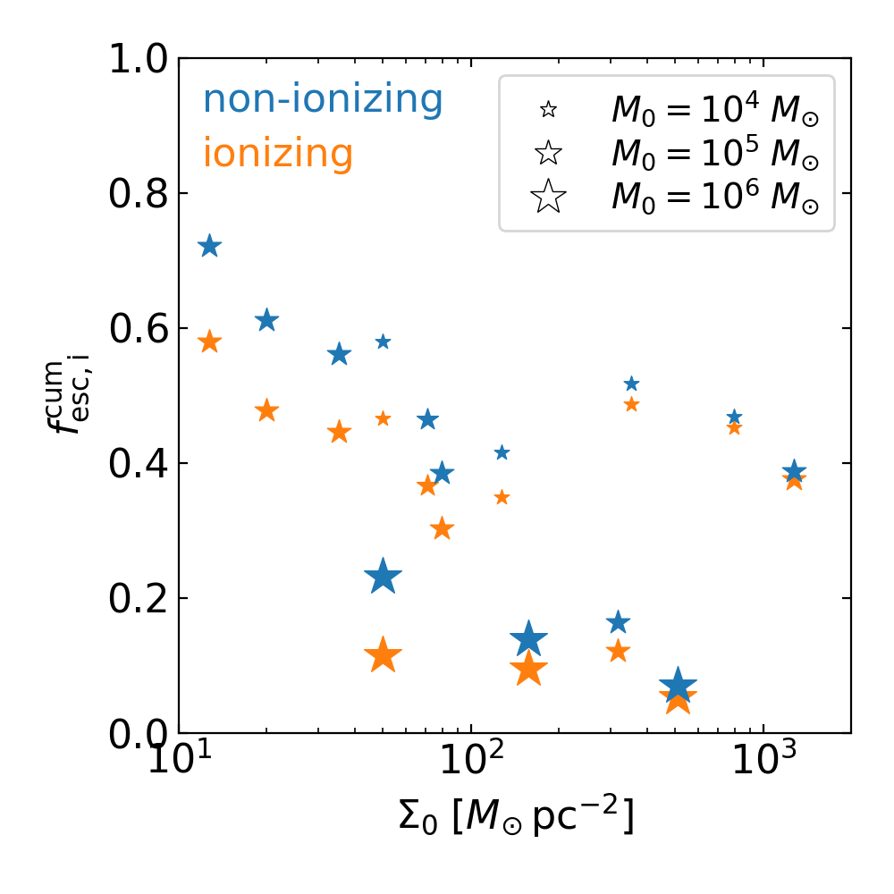
Although our simulations do not account for the time variation of UV luminosity due to stellar evolution, it is worth examining the cumulative fraction of UV photons that escape from the natal cloud up to the time when the first supernova explosions would occur. After this time, impact of SN blasts would affect the cloud structure, and the ionizing photon production rate would drop considerably. Figure 6 plots the cumulative escape fraction of ionizing (orange) and non-ionizing (blue) photons at $t^{\prime}=t-t_{*,0}=3\,{\rm Myr}$ as a function of $\Sigma_{\rm 0}$. These values together with the cumulative dust absorption fractions are also listed in Columns 9–13 of Table 1.

In general, both $f_{\rm esc,i}^{\rm cum}$ and $f_{\rm esc,i}^{\rm cum}$ tend to decrease with increasing $\Sigma_{\rm 0}$, except for models M1E4R02, M1E4R03, and M1E5R05 which have $f_{\rm esc,i}^{\rm cum},f_{\rm esc,n}^{\rm cum}\sim 0.4$–$0.5$. These dense clouds have a short evolutionary timescale, with $t_{\rm dest}<3\,{\rm Myr}$ (see Column 7 of Table 1). In contrast, massive clouds ($M_{\rm 0}=10^{6}\,M_{\odot}$) have a relatively long evolutionary time, and only a tiny fraction of the initial gas mass has been ejected by radiation feedback at $t^{\prime}=3\,{\rm Myr}$ (see Figure 15 in Paper II), leading to very low cumulative escape fractions. Supernova feedback is expected to play a greater role than radiation feedback in destroying these massive clouds. Destruction of these massive clouds by SNe at early times would also increase $f_{\rm esc}^{\rm cum}$ above what is shown in Figure 6 and listed in Table 1.

4 Escape Fraction vs. Optical Depth Distribution

The escape fraction is intrinsically linked to the distribution of optical depth around the sources that emit radiation. In this section, we will first calculate the solid-angle probability distribution function (PDF) of the optical depth as seen from the luminosity center of the sources, and show that its mean and dispersion can be used to predict the escape fraction. Next, we calculate the area PDF of the optical depth projected through the whole cloud as seen by an external observer, and explore ways to estimate the escape fraction using this area PDF. We focus mainly on the escape fraction of non-ionizing radiation since this is determined by the dust optical depth distribution, which can be traced observationally using far-IR thermal dust emission or near-IR extinction mapping (e.g., Lombardi et al., 2014). As demonstrated in Section 3.2, $f_{\rm esc,i}$ is expected to be similar to $f_{\rm esc,n}$.

4.1 Solid Angle-Weighted PDF of Optical Depth

We first provide a general framework to consider escape of radiation from an inhomogeneous cloud, and then we turn to results from our simulations.

For an isotropically emitting point source, the escape fraction of radiation is determined by the solid angle distribution of the optical depth measured from the source. Consider a point source embedded in an isolated dusty cloud with mass $M$ and constant dust opacity per unit mass $\kappa_{\rm d}=\sigma_{\rm d}/\mu_{\rm H}$. The dust optical depth averaged over the solid angle $\Omega$ is

$$\langle\tau^{\rm c}\rangle_{\Omega}=\dfrac{\iint\rho(r,\Omega)\kappa_{\rm d}drd\Omega}{\int d\Omega}\equiv\kappa_{\rm d}\langle\Sigma^{\rm c}\rangle_{\Omega},$$ (8)

where $\rho(r,\Omega)$ is the gas density and $\langle\Sigma^{\rm c}\rangle_{\Omega}=M/(4\pi\bar{r}^{2})$ is the characteristic surface density of the circumsource material with $\bar{r}\equiv(\int r^{-2}dM/\int dM)^{-1/2}$. Here, the superscripts “c” again indicate measurements of circumsource material relative to the cluster center. Let $P_{\Omega}(\ln\,\tau^{\rm c})d\ln\,\tau^{\rm c}=d\Omega/(4\pi)$ denote the fraction of the whole solid angle covered by sightlines with the logarithm of the dust optical depth in the range between $\ln\,\tau^{\rm c}$ and $\ln\,\tau^{\rm c}+d\ln\,\tau^{\rm c}$. The escape fraction of non-ionizing radiation is then given by

$$\langle e^{-\tau^{\rm c}}\rangle_{\Omega}=\int e^{-\tau^{\rm c}}P_{\Omega}(\ln\,\tau^{\rm c})\,d\ln\,\tau^{\rm c}\geq e^{-\langle\tau^{\rm c}\rangle_{\Omega}}\,,$$ (9)

where the inequality follows from $\langle e^{-\tau^{\rm c}}\rangle_{\Omega}=e^{-\langle\tau^{\rm c}\rangle_{\Omega}}\langle e^{-\tau^{\rm c}+\langle\tau^{\rm c}\rangle_{\Omega}}\rangle$ and $\langle e^{-\tau^{\rm c}+\langle\tau^{\rm c}\rangle_{\Omega}}\rangle\geq\langle(1-\tau^{\rm c}+\langle\tau^{\rm c}\rangle_{\Omega}\rangle_{\Omega}=1$. Note that this inequality holds independent of the functional form for the PDF of $\tau^{\rm c}$. Equation (9) states that the true escape fraction $\langle e^{-\tau^{\rm c}}\rangle_{\Omega}$ is always greater than or equal to the naive estimate $e^{-\langle\tau^{\rm c}\rangle_{\Omega}}$ based on the mean optical depth.

Figure 7: (a) Escape fraction of non-ionizing radiation as a function of the solid-angle averaged optical depth $\langle\tau^{\rm c}\rangle_{\Omega}$ seen from the source. With solid lines we show expectations based on lognormal distributions of the optical depth, with standard deviation $\sigma^{\rm c}=0,0.5,\cdots,2.5$ from left to right. (b) The reduction factor $\mathcal{F}$ defined as the ratio of the effective optical depth $\tau_{\rm eff}=-\ln\langle e^{-\tau^{\rm c}}\rangle_{\Omega}$ to $\langle\tau^{\rm c}\rangle_{\Omega}$ as a function of $\sigma^{\rm c}$. The solid lines indicate the reduction factor expected for lognormal distributions with $\langle\tau^{\rm c}\rangle_{\Omega}=0,0.1,1,10,50$, from top to bottom. Small circles in (a) show characteristic escape fraction and in (b) show characteristic reduction factor as measured from each simulation snapshot, where for this purpose we assume that all the sources are gathered at the center of luminosity. Colors correspond to measured value of $\sigma^{\rm c}$ in (a) and $\langle\tau^{c}\rangle_{\Omega}$ in (b).

A broad distribution of the optical depth can make $\langle e^{-\tau^{\rm c}}\rangle_{\Omega}$ much larger than the naive estimate. To demonstrate this, we consider an idealized situation in which $P_{\Omega}$ follows a lognormal distribution

$$P_{\Omega,{\rm LN}}(\ln\tau^{\rm c};\mu^{\rm c},\sigma^{\rm c})\equiv\dfrac{1}{\sqrt{2\pi}\sigma^{\rm c}}\exp\left[-\frac{(\ln\tau^{\rm c}-\mu^{\rm c})^{2}}{2(\sigma^{\rm c})^{2}}\right],$$ (10)

with the mean $\mu^{\rm c}=\langle\ln\tau^{\rm c}\rangle_{\Omega}$ and the standard deviation $\sigma^{\rm c}=\langle(\ln\tau^{\rm c}-\mu^{\rm c})^{2}\rangle_{\Omega}^{1/2}$. The mean optical depth is then given by $\langle\tau^{\rm c}\rangle_{\Omega}=e^{\mu^{\rm c}+(\sigma^{\rm c})^{2}/2}$.

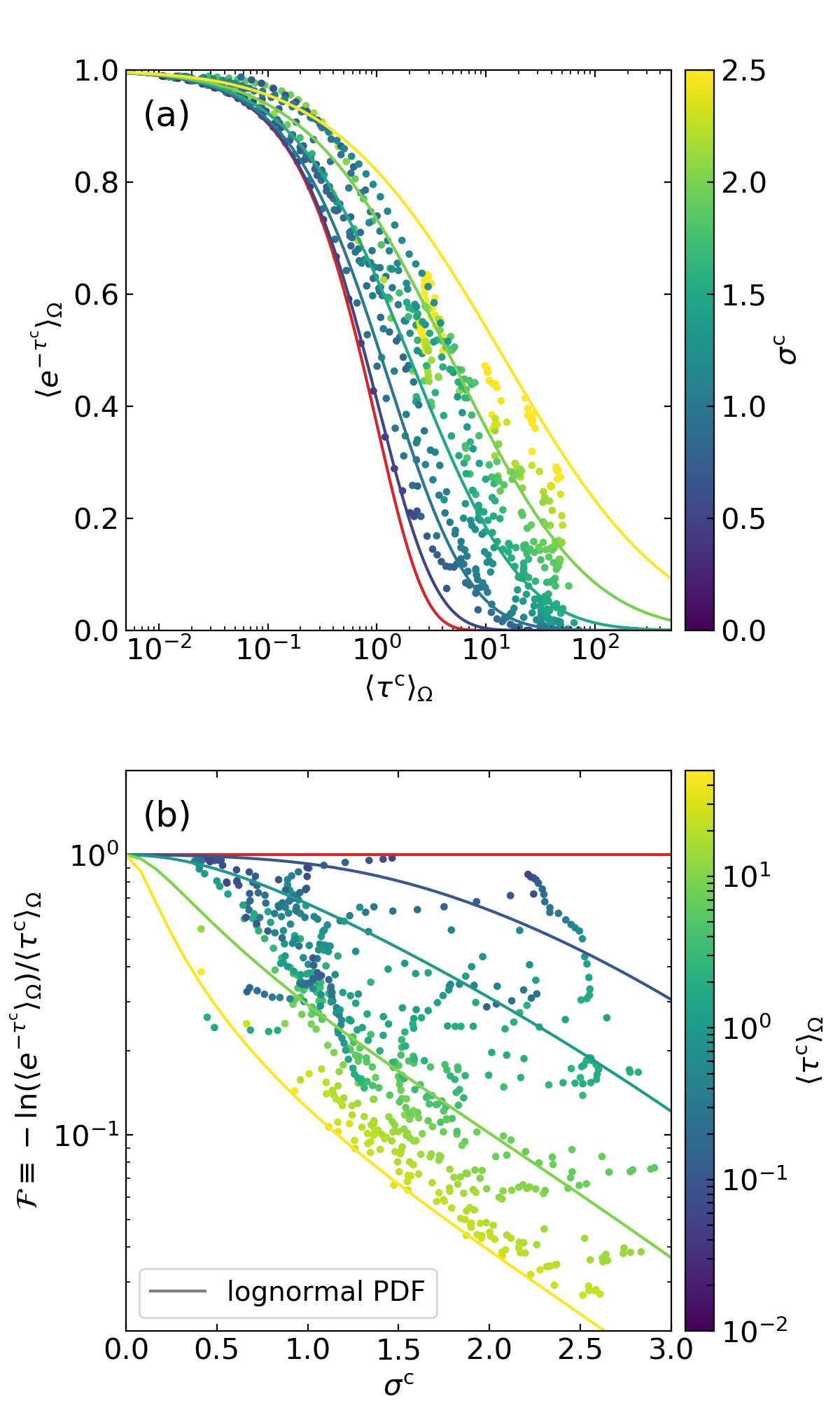
In Figure 7(a) we plot as solid lines the escape fraction $\langle e^{-\tau^{\rm c}}\rangle_{\Omega}$ as a function of $\langle\tau^{\rm c}\rangle_{\Omega}$. All curves are based on lognormal distributions, and each line is colored by its value of $\sigma^{\rm c}$, given by $\sigma^{\rm c}=0,0.5,\cdots,2.5$ from left to right. For $\sigma^{\rm c}\rightarrow 0$, $P_{\Omega}(\ln\tau^{\rm c})$ becomes a delta function and $\langle e^{-\tau^{\rm c}}\rangle_{\Omega}\rightarrow e^{-\langle\tau^{\rm c}\rangle_{\Omega}}$, plotted as the red solid line. Note that the escape fraction is close to unity regardless of $\sigma^{\rm c}$ when $\langle\tau^{\rm c}\rangle_{\Omega}\ll 1$. For $\langle\tau^{\rm c}\rangle_{\Omega}\gtrsim 1$, however, nonzero $\sigma^{\rm c}$ can boost the escape fraction by a large factor relative to the $\sigma^{\rm c}=0$ case. For example, when $\langle\tau^{\rm c}\rangle_{\Omega}=10$, the escape fraction is 0.18 when $\sigma^{\rm c}=1.5$, which is $4000$ times higher than the value $e^{-10}\approx 4.5\times 10^{-5}$ that applies when $\sigma^{\rm c}=0$, since a significant fraction of the sky has $\tau^{\rm c}\lesssim 1$ when the cloud is nonuniform.

The boost of the escape fraction due to inhomogeneous gas distributions around sources corresponds to a reduction in the effective optical depth, $-\ln(\langle e^{-\tau^{\rm c}}\rangle_{\Omega})$. We define the reduction factor

$$\mathcal{F}\equiv-\frac{\ln(\langle e^{-\tau^{\rm c}}\rangle_{\Omega})}{\langle\tau^{\rm c}\rangle_{\Omega}}\leq 1,$$ (11)

which quantifies how much the effective optical depth is reduced relative to the mean optical depth. In Figure 7(b) we plot with solid lines $\mathcal{F}$ as a function of $\sigma^{\rm c}$ for a lognormal PDF with several different values of $\langle\tau^{\rm c}\rangle_{\Omega}$. Curves are colored to indicate the value of $\langle\tau^{\rm c}\rangle_{\Omega}=0,0.1,1,10,50$, from top to bottom. Again, the reduction factor is close to unity regardless of $\sigma^{\rm c}$ for $\langle\tau^{\rm c}\rangle_{\Omega}\ll 1$, but $\mathcal{F}$ can be as small as 0.1 when $\langle\tau^{\rm c}\rangle_{\Omega}\sim 10$ and $\sigma^{\rm c}\sim 2$.

We now turn our attention to $P_{\Omega}(\ln\tau_{\rm n}^{\rm c})$ for our simulation data. For the purpose of measuring a characteristic escape fraction from the cloud in each simulation snapshot, we assume that all radiation is emitted from a single point source located at the stellar center of luminosity $\mathbf{r}_{\rm CL}=\sum_{k}L_{k}\mathbf{r}_{k}/\sum_{k}L_{k}$. We use a trilinear interpolation to remap the density fields $n_{\rm H}$ and $n_{\rm H^{0}}$ from the Cartesian onto a spherical grid with $(N_{r},N_{\theta},N_{\phi})=(128,128,256)$ zones centered at $\mathbf{r}_{\rm CL}$. We set the radial grid spacing to $\Delta r=(2R_{\rm 0}-|\mathbf{r}_{\rm CL}|)/N_{r}$, and calculate the optical depth measured from $\mathbf{r}_{\rm CL}$.

In Figure 7, for all model snapshots we overlay as filled circles (a) the escape fraction of non-ionizing radiation as seen from the center of luminosity against the solid angle-averaged dust optical depth, and (b) the optical-depth reduction factor as a function of the standard deviation of the raw PDFs. As expected, all the data for the escape fraction measurements lie above the red line in (a), corresponding to $\langle e^{-\tau^{\rm c}}\rangle_{\Omega}=e^{-\langle\tau^{\rm c}\rangle_{\Omega}}$, due to finite width of the PDFs. The reduction factor becomes smaller with increasing $\langle\tau^{\rm c}\rangle_{\Omega}$ and $\sigma^{\rm c}$, which is also qualitatively consistent with the lognormal PDF prediction.

Figure 8: (Top) Solid-angle-weighted PDFs of the optical depth for non-ionizing ($\tau_{\rm d}^{\rm c}$, blue) and ionizing ($\tau_{\rm i}^{\rm c}$, orange) radiation measured from the stellar center of luminosity for the fiducial model at $0.5$, $1.5$, $3$, and $5\,{\rm Myr}$ after the first epoch of star formation. (Bottom) Area-weighted PDFs of the optical depth projected along the three principal axes for non-ionizing ($\tau_{\rm d}^{\rm ext}$, blue) and ionizing ($\tau_{\rm i}^{\rm ext}$, orange) radiation within the half-mass radius $R_{\rm h}$.

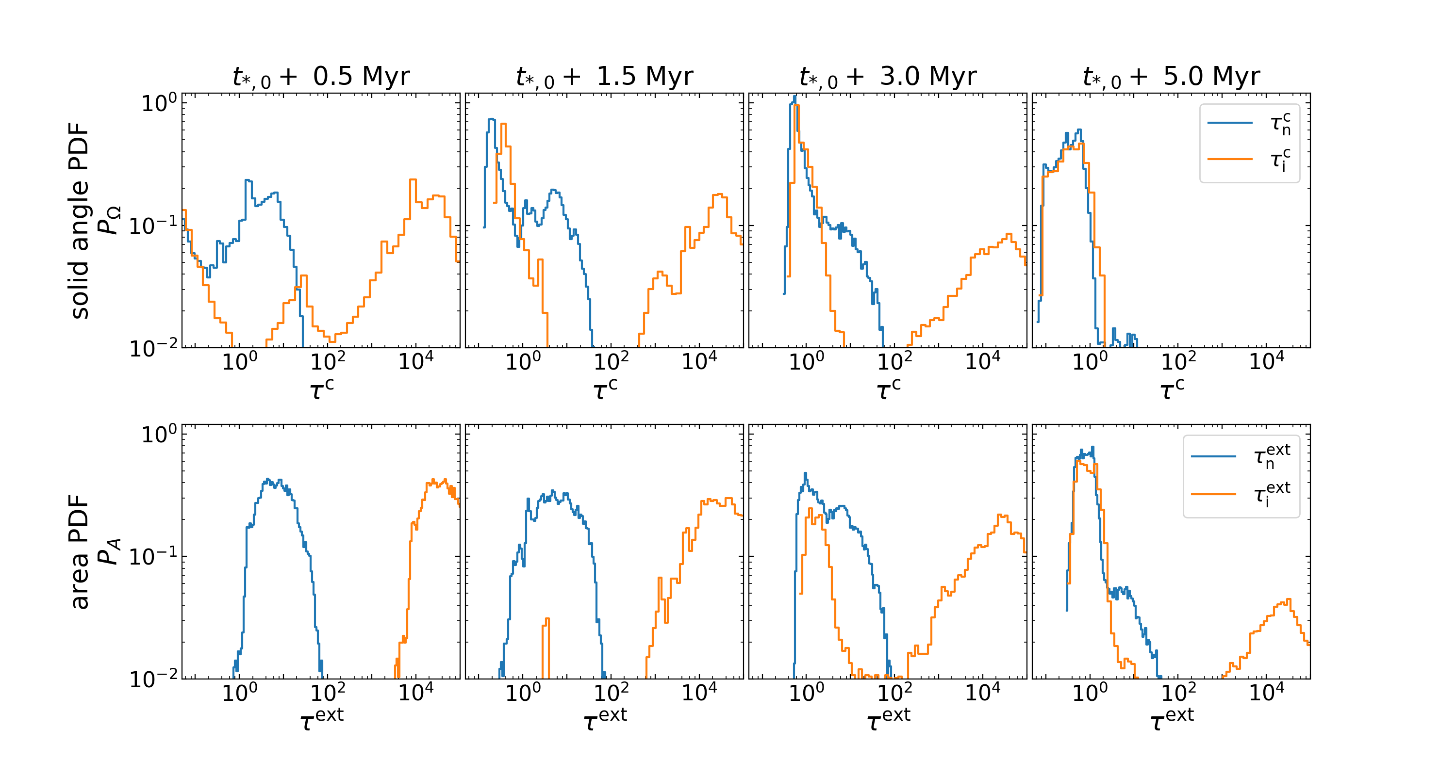
The top row of Figure 8 plots the solid-angle PDFs of the optical depth for non-ionizing (blue) and ionizing (orange) radiation, as measured from the center of luminosity for the fiducial model at the four different times shown in Figure 1. The PDFs, in general, do not look like lognormal distributions, with multiple peaks and shoulders associated with low-density holes and dense neutral clumps. Except at very late times, the solid-angle PDF for ionizing radiation is typically bimodal, while for non-ionizing radiation the solid-angle PDFs are unimodal.

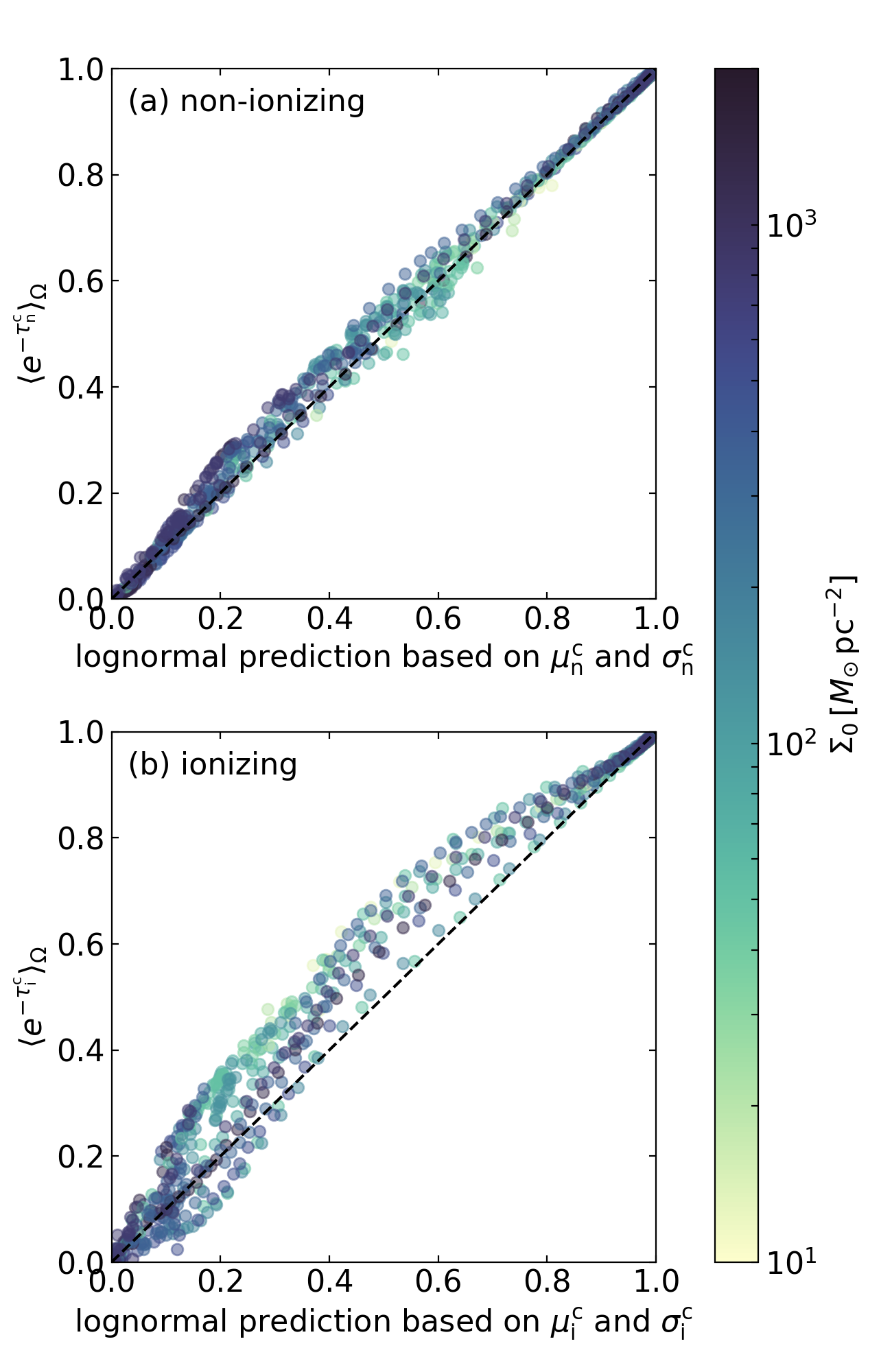
For each simulation snapshot in all models, we measure the mean $\mu^{\rm c}$ and standard deviation $\sigma^{\rm c}$ from the raw PDFs, for both ionizing and non-ionizing radiation. We then calculate what the escape fraction would be using Equation (9) with a lognormal (Equation 10) for $P_{\Omega}(\ln\tau^{\rm c})$, using the measured $\mu^{\rm c}$ and $\sigma^{\rm c}$ values. We also directly evaluate Equation (9) using the raw PDF for $P_{\Omega}(\ln\tau^{\rm c})$ to obtain the true escape fraction $\langle e^{-\tau^{\rm c}}\rangle_{\Omega}$ from the luminosity center. Figure 9 compares the true escape fractions with the estimated escape fractions based on lognormals with the same $\mu^{\rm c}$ and $\sigma^{\rm c}$, for all simulation snapshots. We show results for both (a) non-ionizing and (b) ionizing radiation. The lognormal estimate agrees with the raw escape fraction within $7\%$ for non-ionizing and within $20\%$ for ionizing radiation. This suggests that quite a good estimate of the escape fraction can be obtained given knowledge of the mean and variance in $\ln\tau^{\rm c}$. The superiority of the estimated escape fraction for non-ionizing radiation compared to ionizing radiation is not surprising, given that the former is typically closer to a lognormal (as the example in Figure 8 shows), but our results demonstrate that the escape fraction is insensitive to the detailed functional form of the PDF.

The temporal evolution of $\langle e^{-\tau_{\rm i}^{\rm c}}\rangle_{\Omega}$ and $\langle e^{-\tau_{\rm n}^{\rm c}}\rangle_{\Omega}$ for some selected models are plotted as dotted and dashed lines in Figure 5. Overall, these agree quite well with the luminosity-weighted escape fractions $f_{\rm esc,n}$ and $f_{\rm esc,i}$, suggesting that distributed sources can be regarded as if they were gathered at the luminosity center for the purpose of calculating the photon escape fractions. We note that the predicted escape fraction from a single source is somewhat larger than the actual escape fraction in the early phase of evolution. This is because at early time sources are clustered in a few widely-separated regions (e.g., leftmost column of Figure 1) and the luminosity center is located in a low-density void created by turbulence, in which case the gas distribution around the luminosity center does not properly represent the actual gas distributions surrounding individual sources.

Figure 9: Comparison of the true escape fraction as seen from the cluster center with an estimated escape fraction for (a) non-ionizing and (b) ionizing radiation, for all simulation snapshots. The true escape fraction $\langle e^{-\tau^{\rm c}}\rangle_{\Omega}$ on the ordinate is calculated from Equation (9) using the raw PDF for $P_{\Omega}$. The estimated escape fraction on the abscissa uses Equation (10) for $P_{\Omega}$, with the mean (${\mu}^{\rm c}$) and width (${\sigma}^{\rm c}$) as measured from the raw solid-angle PDF.

4.2 Area-Weighted PDF of Optical Depth

While the solid-angle PDF of the optical depth, $P_{\Omega}(\tau^{\rm c})$, determines the escape fraction, it is not directly available to an external observer. At best, several individual line-of-sight values of $\tau^{\rm c}$ could be obtained from spectral observations of stars within a cloud. If the H II region is well resolved, sampling of multiwavelength nebular spectra in sufficiently many locations could also be used to estimate the distribution of optical depths e.g., using the Balmer decrement method. Alternatively, given sufficient resolving power, an external observer could use IR dust extinction or emission maps to measure the area distribution, $P_{A}(\tau_{\rm n}^{\rm ext})$, of the dust optical depth $\tau_{\rm n}^{\rm ext}$ projected on the plane of the sky. Can the observer use $P_{A}(\tau_{\rm n}^{\rm ext})$ to obtain an estimate of the escape fraction close to the real value? We explore this possibility below.

Since the area PDF defined over the entire domain depends on the box size, we consider the gas only within the half-mass radius of the cloud as follows. We first calculate the column-density weighted mean position of a gas cloud with total mass $M_{\rm gas}$, and take it as the cloud center in the projected plane of the sky (cross symbols in the top row of Figures 1 and 2). Next, we draw a circle with the half-mass radius $R_{\rm h}$ about the center that encloses 50% of the total gas mass (dotted circles in the top row of Figures 1 and 2). This allows us to define the area-averaged surface density $\langle\Sigma^{\rm ext}\rangle_{A}\equiv\tfrac{1}{2}{M_{\rm gas}}/(\pi R_{\rm h}^{2})$ and the area-averaged non-ionizing (dust) optical depth $\langle\tau_{\rm n}^{\rm ext}\rangle_{A}=\kappa_{\rm d}\langle\Sigma^{\rm ext}\rangle_{A}$ within the half-mass radius. We post-process all snapshots in the time range ($t_{*,0},t_{\rm ej,99\%}$) at $0.05t_{\rm ff,0}$ interval, where $t_{\rm ej,99\%}$ denotes the time at which 99% of initial gas mass has been ejected from the simulation domain.

The bottom row of Figure 8 plots as blue lines the area-weighted PDFs of the dust optical depth within the half-mass radius in the fiducial model, at four different times shown in Figure 1. The PDFs along the three principal ($x$, $y$, and $z$) axes are combined. At $t^{\prime}=0.5\,{\rm Myr}$, the area PDF is approximately lognormal since the density distribution is dominated by supersonic turbulence (e.g., McKee & Ostriker, 2007). The fraction of area with low $\tau_{\rm n}^{\rm ext}$ grows over time due to photoevaporation. At $t^{\prime}=5\,{\rm Myr}$, the area PDF exhibits a narrow width and a pronounced peak at $\tau_{\rm n}^{\rm ext}\sim 1$.

In the bottom row of Figure 8, we also plot as orange lines the area-weighted PDFs of the projected optical depth for ionizing radiation $\tau_{\rm i}^{\rm ext}=\int(n_{\rm H}\sigma_{\rm d}+n_{\rm H^{0}}\sigma_{\rm ph})\,dz$. At early times, the area PDF of $\tau_{\rm i}^{\rm ext}$ is largely similar in shape to the PDF of $\tau_{\rm n}^{\rm ext}$ with a shift to the right by a factor $\sigma_{\rm ph}/\sigma_{\rm d}$ because only a tiny fraction of sightlines are optically thin and $\tau_{\rm i}\sim\tau_{\rm d}(\sigma_{\rm ph}/\sigma_{\rm d})$ along most sightlines. At intermediate times, the area-weighted PDFs of $\tau_{\rm i}^{\rm ext}$ have two peaks and shoulders associated with neutral clumps and ionized interclump gas. Later, the PDFs for $\tau_{\rm i}$ and $\tau_{\rm n}$ become similar as neutral gas covers only a tiny fraction of the total area within $R_{\rm h}$ and most sightlines have $x_{\rm n}\lesssim\sigma_{\rm d}/\sigma_{\rm ph}$.

Figure 10: Instantaneous escape fraction $f_{\rm esc,n}$ of non-ionizing radiation against the area-averaged dust optical depth $\langle\tau^{\rm ext}_{\rm n}\rangle_{A}$ within the half-mass radius for all models. The color of each dot indicates the initial surface density of the cloud. The horizontal bars represent the 1-sigma uncertainty based on $\langle\tau^{\rm ext}_{\rm n}\rangle_{A}$ measured along three different orientations. Red dashed lines provided for comparison correspond to $f_{\rm esc,n}=e^{-\langle\tau_{\rm n}^{\rm ext}\rangle_{A}}$, $e^{-0.1\langle\tau_{\rm n}^{\rm ext}\rangle_{A}}$, and $e^{-0.01\langle\tau_{\rm n}^{\rm ext}\rangle_{A}}$ from left to right. This shows that the effective optical depth for escape of photons is much lower than the value implied by the mean column of gas in the cloud. The estimate of escape fraction $f_{\rm esc,n}^{\rm est,1}$ is shown with a solid red curve (see Equation 12).

4.2.1 Estimation of $f_{\rm esc,n}$

Figure 11: Area-averaged dust optical depth $\langle\tau_{\rm n}^{\rm ext}\rangle_{A}$ within the half-mass radius vs. the reduction factor $\mathcal{F}^{\rm ext}\equiv-\ln\,(f_{\rm esc,n})/\langle\tau_{\rm n}^{\rm ext}\rangle_{A}$ for an external observer for all models. The error bars show the standard deviation of measurements along three projection directions. The effective optical depth for photons escaping from embedded clusters is reduced by a factor $\sim 0.5$ (at low $\langle\tau_{\rm n}^{\rm ext}\rangle_{A}$) to $\sim 0.02$ (at high $\langle\tau_{\rm n}^{\rm ext}\rangle_{A}$) compared to the mean cloud optical depth $\langle\tau_{\rm n}^{\rm ext}\rangle_{A}$ seen by an external observer.

Figure 12: Actual escape fraction $f_{\rm esc,n}$ of non-ionizing radiation vs. estimated escape fraction (a) based on the area-averaged optical depth $f_{\rm esc,n}^{\rm est,1}=\exp(-\eta_{1}\langle\tau_{\rm n}^{\rm ext}\rangle_{A})$ with $\eta_{1}=0.56/(1+1.25\langle\tau_{\rm n}^{\rm ext}\rangle_{A}^{0.48})$ and (b) the area-averaged escape fraction $f_{\rm esc,n}^{\rm est,2}=\langle\exp(-\eta_{2}\tau_{\rm n}^{\rm ext})\rangle_{A}$ with $\eta_{2}=0.30$. The dashed lines draw $f_{\rm esc,n}/f_{\rm esc,n}^{\rm est}=1$.

Marginally-resolved Cloud Case

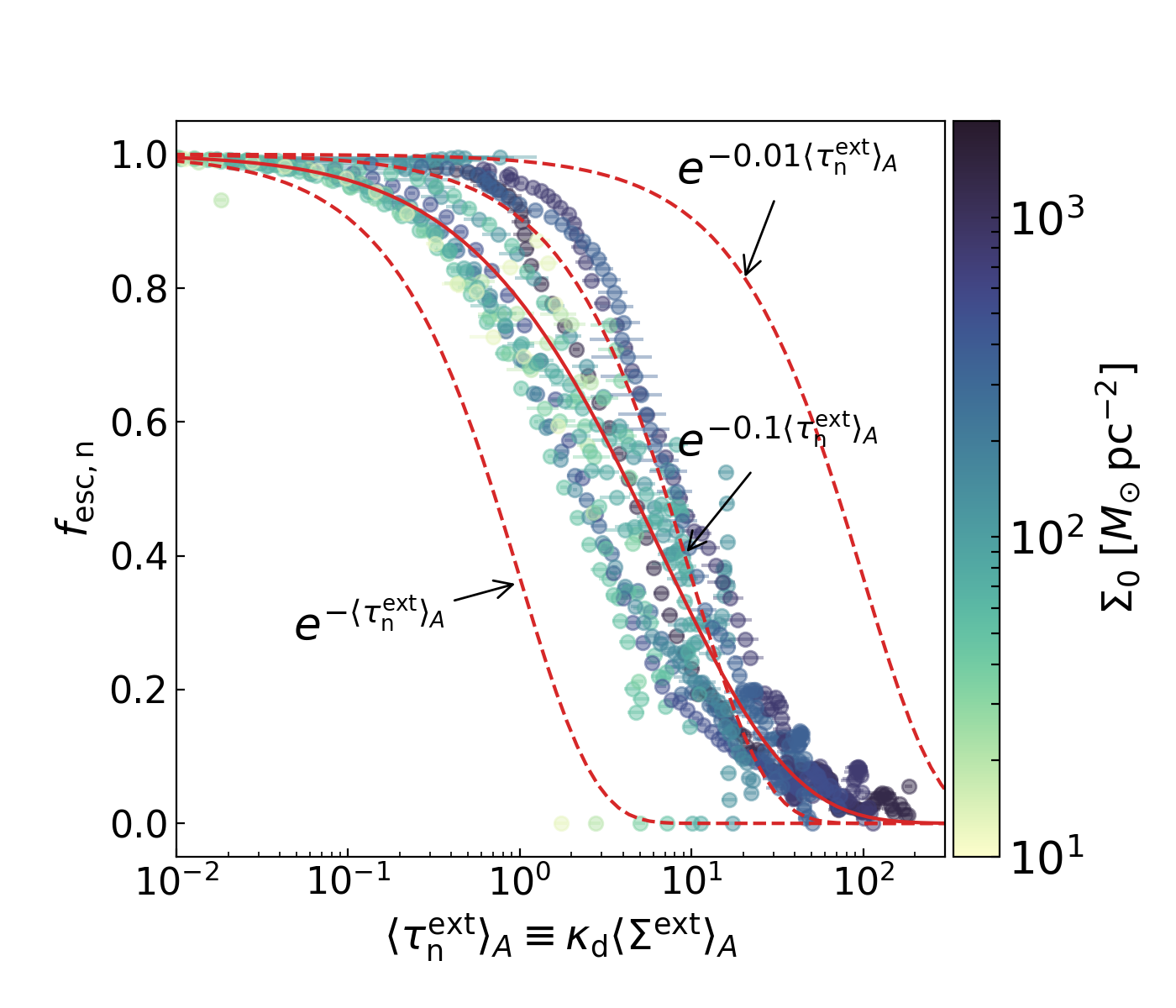
The simplest estimate of the escape fraction would make use of the mean column of dust in a cloud, averaged over the aperture. This would be useful for a cloud that is distant and not well resolved. Figure 10 plots the instantaneous escape fractions $f_{\rm esc,n}$ of non-ionizing radiation as a function of the area-averaged optical depth $\langle\tau_{\rm n}^{\rm ext}\rangle_{A}$ for all models, with the color representing the initial cloud surface density. The circles show the median value of $\langle\tau_{\rm n}^{\rm ext}\rangle_{A}$ measured along the three principal axes, while the horizontal bars indicate the sample standard deviation, which is typically $\sim 20$–$30\%$ of $\langle\tau_{\rm n}^{\rm ext}\rangle_{A}$. Note that all clouds start from $\langle\Sigma^{\rm ext}\rangle_{A}\sim\Sigma_{\rm 0}$ and evolve towards a state with $\langle\Sigma^{\rm ext}\rangle_{A}\rightarrow 0$ and $f_{\rm esc,n}\rightarrow 1$. For comparison, we plot as red dashed lines the simple predictions assuming that the optical depth is equal to the mean value within the half-mass radius, or is reduced by a factor of $10$ or $100$, i.e. $e^{-\langle\tau_{\rm n}^{\rm ext}\rangle_{A}}$, $e^{-0.1\langle\tau_{\rm n}^{\rm ext}\rangle_{A}}$, and $e^{-0.01\langle\tau_{\rm n}^{\rm ext}\rangle_{A}}$ from left to right.

Figure 10 shows that the actual escape fraction is significantly higher than the naive estimate $e^{-\langle\tau_{\rm n}^{\rm ext}\rangle_{A}}$. The reason is twofold. First, using just a single mean optical depth does not account for the variance associated with turbulence-driven structure, and leads to an underestimate of the escape fraction for the reasons explained in Section 4.1. Second, even the area-averaged optical depth measured by an external observer would be higher than the solid angle-averaged optical depth measured by an internal observer located at the luminosity center. For example, a uniform density sphere with radius $R$ and density $\rho$ has a half-mass radius $R_{\rm h}=(1-2^{-2/3})^{1/2}R$ so that $\langle\tau_{\rm n}^{\rm ext}\rangle_{A}=1.8\rho R\kappa_{\rm d}$, nearly a factor two larger than $\tau^{\rm c}_{\rm n}$. While not as extreme in turbulent clouds, Figure 8 shows that the mean $\langle\tau_{\rm n}^{\rm ext}\rangle_{A}$ of the area PDF is larger than the mean $\langle\tau_{\rm n}^{\rm c}\rangle_{\Omega}$ of the solid angle PDF.

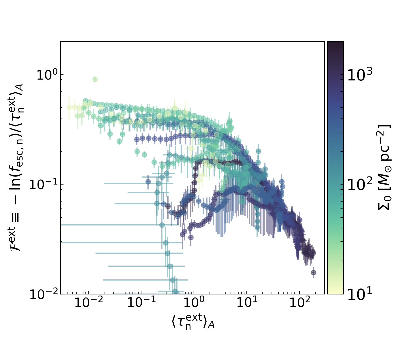
The results in Figure 10 suggest that an approximate estimate of the escape fraction may be obtained by applying an appropriate reduction factor to $\langle\tau_{\rm n}^{\rm ext}\rangle_{A}$. Similar to Equation (11), we define the reduction factor $\mathcal{F}^{\rm ext}\equiv-\ln\,(f_{\rm esc,n})/\langle\tau_{\rm n}^{\rm ext}\rangle_{A}$ for an external observer. It tells us what the reduction in the effective optical depth is relative to the area-averaged optical depth $\langle\tau_{\rm n}^{\rm ext}\rangle_{A}$ and depends both on the geometric distribution of gas and stars and (weakly) on the viewing angle of the observer. Figure 11 plots as circles $\mathcal{F}^{\rm ext}$ as a function of $\langle\tau_{\rm n}^{\rm ext}\rangle_{A}$ with error bars indicating the standard deviation of the values measured along three principal axes. The reduction tends to be more significant for snapshots with larger $\langle\tau_{\rm n}^{\rm ext}\rangle_{A}$, similar to the trend we found for $\mathcal{F}$ in Figure 7 (see also Figure 14 in Appendix). In the limit $\langle\tau_{\rm n}^{\rm ext}\rangle_{A}\ll 1$, the reduction factor tends to the geometric correction factor $\sim 1/1.8$ for uniform density sphere.

Based on the above findings, we estimate the escape fraction as

$$f_{\rm esc,n}^{\rm est,1}=\exp\left(-\eta_{1}\langle\tau_{\rm n}^{\rm ext}\rangle_{A}\right)\,.$$ (12)

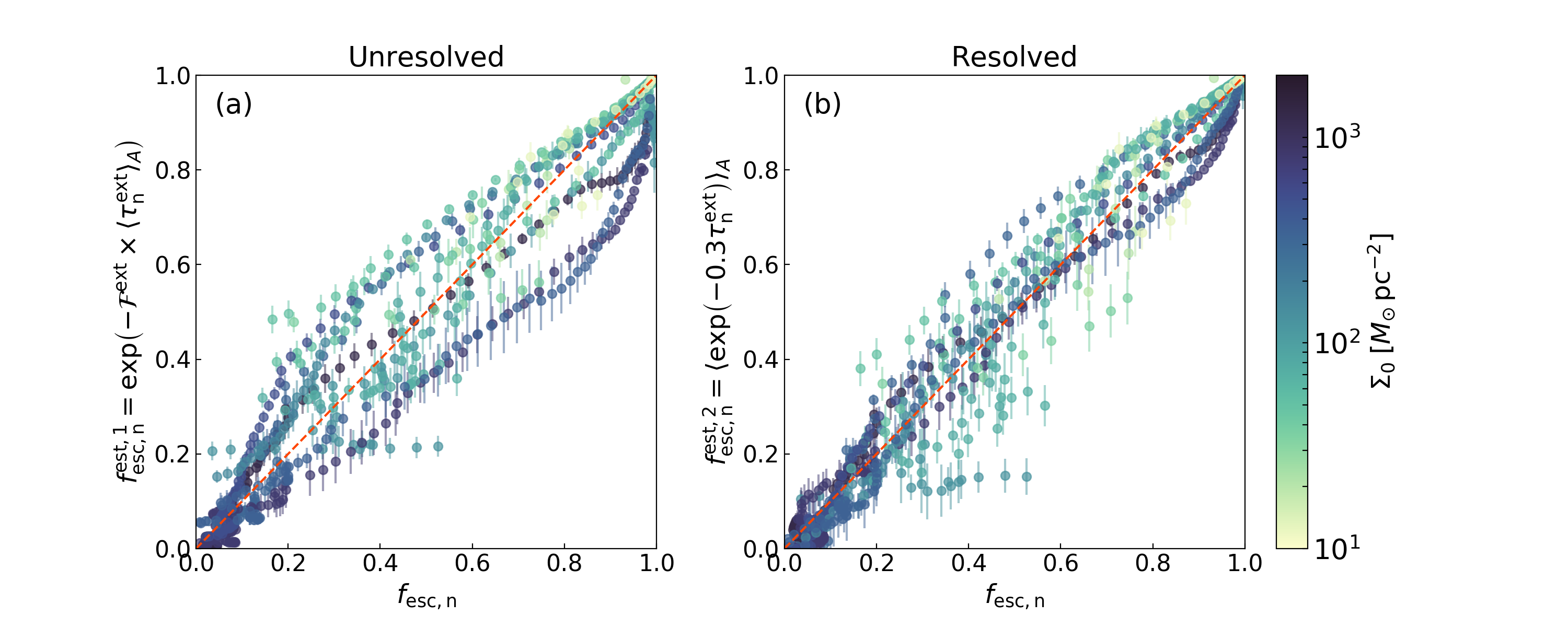
As an estimate of a correction factor $\mathcal{F}^{\rm ext}$ based only on information that would be available for a marginally-resolved cloud, we adopt a functional form $\eta_{1}=\tfrac{1/1.8}{1+a\langle\tau_{\rm n}^{\rm ext}\rangle_{A}^{b}}$, with constants $a$ and $b$ to be determined. The estimate in Equation (12) depends only on $\langle\tau_{\rm n}^{\rm ext}\rangle_{A}$ and approaches $\eta_{1}\rightarrow 1/1.8$ for $\langle\tau_{\rm n}^{\rm ext}\rangle_{A}\rightarrow 0$. We perform a least square fit to find parameters $a=1.25$, $b=0.48$ that minimize the sum of squared errors ($(f_{\rm esc,n}-f_{\rm esc,n}^{\rm est,1})^{2}$) compared to our simulation results. Figure 12(a) compares the actual escape fraction $f_{\rm esc,n}$ of non-ionizing radiation and $f_{\rm esc,n}^{\rm est,1}=\exp\left(\tfrac{-0.56\langle\tau_{\rm n}^{\rm ext}\rangle_{A}}{1+1.25\langle\tau_{\rm n}^{\rm ext}\rangle_{A}^{0.48}}\right)$ for all models, with color corresponding to the initial cloud surface density. This estimator predicts $f_{\rm esc,n}$ within $\sim 20\%$. The estimator of Equation (12) is also shown as a red solid line in Figure 10).

Resolved Cloud Case

We have also tested a second method to estimate the escape fraction assuming that the area PDF of $\tau_{\rm n}^{\rm ext}$ is available. In this approach, one may estimate the escape fraction by taking the direct area average

$$f_{\rm esc,n}^{\rm est,2}=\langle\exp(-\eta_{2}\tau_{\rm n}^{\rm ext})\rangle_{A}\,,$$ (13)

where $\eta_{2}$ is a constant correction factor. To find the optimal value of $\eta_{2}$, we calculate the individual correction factor $\eta$ that gives $\langle\exp(-\eta\tau_{\rm n}^{\rm ext})\rangle_{A}=f_{\rm esc,n}$ for each snapshot of all simulations. The resulting $\eta$ values range between 0.1 and 0.5, with an average value of 0.30 and standard deviation of 0.14. We also adopt the constant value of $\eta_{2}$ for all snapshots and find that $\eta_{2}=0.30$ minimizes the sum of the square of the differences $(f_{\rm esc,n}^{\rm est,2}-f_{\rm esc,n})^{2}$. Figure 12(b) compares $f_{\rm esc,n}^{\rm est,2}$ with the actual escape fraction, again showing that this method predicts $f_{\rm esc,n}$ within 20%.

These results indicate that the two methods based on externally-observed mean dust optical depth or optical depth distribution around a young star cluster can be reliably used to infer the actual escape fraction from the cluster. Although the largest errors are comparable for the two methods, the mean errors are smaller using the second method. This implies that more accurate estimates of the escape fraction may be obtained when the resolved dust distribution (or gas distribution, with an assumed dust-to-gas value) can be measured.

5 Summary and Discussion

5.1 Summary

Stellar UV photons escaping from star-forming regions have a profound influence on the ISM, especially its thermal and chemical state, together with the resulting dynamical evolution including star formation. Despite this importance, the escape fraction has not previously been well characterized in observations, and theoretical predictions are also lacking. In this work, we have used a suite of radiation hydrodynamic simulations to study the evolution of the escape fractions $f_{\rm esc,n}$ and $f_{\rm esc,i}$ for both non-ionizing and ionizing radiation, and to analyze in detail how the escape fraction depends on the dust optical depth distribution. Our simulations span a range of physical conditions and include the effects of photoionization and radiation pressure from UV radiation, but do not consider stellar evolution and other forms of stellar feedback such as stellar winds or supernovae.

Utilizing the adaptive ray tracing module, we accurately follow the propagation of ionizing and non-ionizing radiation from multiple sources and monitor temporal evolution of the escape fraction, the dust absorption fraction, and the hydrogen absorption fraction. We also explore how the escape fraction is related to the solid-angle weighted distribution of the optical depth as seen from the center of sources, and to the area-weighted distribution of the optical depth as seen from outside the cloud. Based on our results, we propose two methods to estimate the escape fraction from the observed optical depth in the plane of sky.

Our key findings are summarized below.

1. Temporal Evolution

   In all of our simulations, the escape fraction increases with time and becomes unity within a few free-fall times after the onset of feedback (Figures 3 and 5). While clouds with low surface density are dispersed by radiation feedback rather quickly in a single free-fall time (Figures 1 and 3), H II regions formed in clouds with high surface density spend a long embedded-phase ($\sim 2$–$3t_{\rm ff,0}$) during which the escape fraction of ionizing radiation is small ($f_{\rm esc,i}\lesssim 0.1$), while the hydrogen absorption fraction ($f_{\rm gas,i}$) remains high (Figures 2 and 3). Overall, $f_{\rm gas,i}$ decreases more-or-less monotonically with time, while the dust absorption fraction of ionizing photons ($f_{\rm dust,i}$) reaches a peak slightly before the cloud destruction and decreases in the late evolutionary phase (Figure 3). The escape of both ionizing and non-ionizing radiation occurs mainly through low-density regions, along directions for which the H II region is density-bounded (Figures 1 and  2). As a result, the difference between the escape fraction of non-ionizing ($f_{\rm esc,n}$) and ionizing radiation is quite small or only modest (Figure 5), with the dust absorption controlling the escape of UV radiation in the late phase.

2. Comparison to Semi-analytic Models for Spherical, Embedded H II Regions

   Previous theoretical models for spherical, static, and embedded H II regions with $f_{\rm esc,i}=0$ have predicted that $f_{\rm gas,i}=Q_{\rm gas,i}/Q_{\rm i}$ increases (and $f_{\rm dust,i}$ decreases) with increasing $Q_{\rm gas,i}n_{\rm i,rms}$, where $Q_{\rm gas,i}$ is the absorption rate of ionizing photons by hydrogen and $n_{\rm i,rms}$ is the rms number density of ionized gas inside an H II region. In our simulations, however, the relationship between $f_{\rm gas,i}$ (or $f_{\rm dust,i}$) and $Q_{\rm gas,i}n_{\rm i,rms}$ depends on the evolutionary phase of an H II region, and deviates considerably from the theoretical predictions (Figure 4). The discrepancy between the spherical model prediction and our numerical results is caused by the fact that H II regions in our simulations are highly non-uniform and subject to loss of ionizing radiation through optically-thin holes, and that in time-dependent flows ionization rates can be enhanced by “fresh” neutral gas. The range of $f_{\rm gas,i}$ in our simulations is consistent with observed estimates in galactic H II regions.

3. Cumulative Escape Fraction Before First Supernovae

   The cumulative escape fraction of ionizing photons ($f_{\rm esc,i}^{\rm cum}$) before the time of the first supernovae ($3\,{\rm Myr}$ after the onset of radiation feedback) ranges from 5% to 58% (Table 1). The range of $f_{\rm esc,n}^{\rm cum}$ for non-ionizing photons is 7% to 72%. For fixed cloud mass, and both EUV and FUV, $f_{\rm esc}^{\rm cum}(3\,{\rm Myr})$ tends to decrease with increasing $\Sigma_{\rm 0}$ (Figure 6). At a given $\Sigma_{\rm 0}$, large, massive clouds have smaller $f_{\rm esc}^{\rm cum}(3\,{\rm Myr})$ than compact, less massive clouds owing to longer evolutionary timescales. Dense, cluster-forming clumps that are destroyed within $3\,{\rm Myr}$ (M1E4R03, M1E4R02, and M1E5R05) have relatively high values of $f_{\rm esc}^{\rm cum}(3\,{\rm Myr})\sim 40\%$–$50\%$.

4. Solid-Angle Weighted Optical Depth PDF

   For an isotropic point source of radiation, the escape fraction is determined by the solid-angle weighted PDF $P_{\Omega}$ of the optical depth as seen from the point source through Equation (9). Assuming that $P_{\Omega}$ is lognormal, we demonstrate that the point-source escape fraction $\langle e^{-\tau^{\rm c}}\rangle_{\Omega}$ is much higher than would be estimated based on the solid-angle averaged optical depth, ($e^{-\langle\tau^{\rm c}\rangle_{\Omega}}$), if the PDF has a large dispersion $\sigma^{\rm c}$ (Figure 7). We calculate $P_{\Omega}$ in our simulations by assuming that all radiation is emitted from the luminosity center of source particles. The shape of $P_{\Omega}$ is in general not lognormal, with peaks and dips associated with dense, star-forming clumps and photoevaporated, outflowing gas (top row of Figure 8). Nevertheless, the lognormal estimates based on the mean and standard deviation of $P_{\Omega}$ are quite close to the true escape fraction $\langle e^{-\tau^{\rm c}}\rangle_{\Omega}$ from the luminosity center (Figure 9). We define the reduction factor $\mathcal{F}=-\ln(\langle e^{-\tau^{\rm c}}\rangle_{\Omega})/\langle\tau^{\rm c}\rangle_{\Omega}$ that measures the effective optical depth relative to the mean value for non-ionizing radiation. We show that $\mathcal{F}$ decreases as $\langle\tau^{\rm c}\rangle_{\Omega}$ and/or $\sigma^{\rm c}$ increases (Figure 7).

5. Area Weighted Optical Depth PDF

   We calculate the area-weighted PDF $P_{A}$ of the optical depth within the half-mass radius of gas, as would be measured by an external observer, finding that the shape and temporal change of $P_{A}$ are similar to those of the solid-angle PDF $P_{\Omega}$ (Figure 8). Consistent with results from the solid-angle PDF, a simple estimate of the escape fraction ($e^{-\langle\tau^{\rm ext}_{\rm n}\rangle_{A}}$) based on the area-averaged optical depth $\langle\tau^{\rm ext}\rangle_{A}$ significantly underestimates the real escape fraction (Figure 10). This is because $\langle\tau^{\rm ext}\rangle_{A}$ is higher than $\langle\tau^{\rm c}\rangle_{\Omega}$ measured from the luminosity center (due to path length differences) and does not properly account for the variance in optical depth; the latter is more important at high optical depth. The reduction in the effective optical depth tends is quite dramatic for larger $\langle\tau^{\rm ext}_{\rm n}\rangle_{A}$ (Figure 11), such that the effective optical depth is $\sim 1$ when $\langle\tau^{\rm ext}\rangle_{A}\sim 10$.

   We present two simple methods for estimating $f_{\rm esc,n}$ for observed star-forming regions. In the first method, we assume a marginally resolved cloud for which only the area-averaged dust optical depth $\langle\tau^{\rm ext}\rangle_{A}$ is observationally available. We show that our results agree with the estimate of the escape fraction $f_{\rm esc,n}^{\rm est,1}=e^{-\eta_{1}\langle\tau^{\rm ext}\rangle_{A}}$, where the correction factor $\eta_{1}=0.56/(1+1.25\langle\tau^{\rm ext}\rangle_{A}^{0.48})$ depends only on $\langle\tau^{\rm ext}\rangle_{A}$. In the second method, we assume that the area distribution $P_{A}$ of the dust optical depth $\tau^{\rm ext}_{\rm n}$ surrounding sources is observationally available. We show that our results agree well with the estimate based on an area average, $f_{\rm esc,n}^{\rm est,2}=\langle e^{-\eta_{2}\tau^{\rm ext}_{\rm n}}\rangle_{A}$ with a constant correction factor $\eta_{2}=0.3$. The two methods both yield estimates within $\sim 20\%$ of the actual luminosity-weighted escape fraction obtained from adaptive ray tracing in our simulations (Figure 12).

5.2 Discussion

5.2.1 Comparison with Other Simulations

In previous work, we compared radiation fields computed from a two-moment radiation scheme with $M_{1}$-closure relation with those computed with ART for identical distributions of sources and gas density, and found that the two methods are in good agreement with each other in terms of large-scale radiation field and escape fraction (Paper I). One would therefore expect similar results for $f_{\rm esc,n}$ to the findings reported in Raskutti et al. (2017), which used the $M_{1}$ scheme to study the interaction between non-ionizing radiation and gas using the same basic cloud model as we adopt here (see Raskutti et al., 2016, but note specific model parameters differ). In practice, however, it is not meaningful to make a detailed comparison because the evolution of SFE with time diverges between simulations that use ART and those that use M1. Paper II compared our ART simulations with the results of Raskutti et al. (2016) and showed that use of the $M_{1}$ method can overestimate the SFE, since radiation forces are underestimated in the vicinity of star particles. Thus, while trends of cumulative $f_{\rm esc,n}$ with cloud properties are quite similar here to those reported in Raskutti et al. (2017), specific models cannot be directly compared.

It is even more difficult to make comparisons of escape fractions with other simulations in which not just the radiative transfer scheme but also cloud parameters, treatment of sink/source particles, dust opacity, and feedback mechanisms are quite different from those we have considered. Nevertheless, it is noteworthy to observe that there is a consistent common trend among different studies of decreasing cumulative (or instantaneous) LyC escape fraction at the time of the first supernovae with increasing cloud mass. In our simulations, low-mass clouds that evolve rapidly ($t_{\rm ff,0}<1\,{\rm Myr}$) and are destroyed before $t^{\prime}=3\,{\rm Myr}$ have $f_{\rm esc,i}^{\rm cum}(3\,{\rm Myr})\gtrsim 0.4$, while massive ($M_{\rm 0}=10^{6}\,M_{\odot}$) clouds with $t_{\rm ff,0}\gtrsim 5\,{\rm Myr}$ have $f_{\rm esc,i}^{\rm cum}(3\,{\rm Myr})\sim 0.1$ (see Section 3.3 and Table 1). Likewise, Dale et al. (2012) found that dense, compact clouds (their Runs F, I, J) exhibit $f_{\rm esc,i}\gtrsim 0.8$ at the time of the first supernovae, whereas massive ($M_{\rm 0}=10^{6}\,M_{\odot}$) clouds (their Runs A, B, X) have $f_{\rm esc,i}\lesssim 0.2$. Kimm et al. (2019) report that the luminosity-weighted, time-averaged escape fraction is only $5.2\%$ for a solar-metallicity cloud with $M_{\rm 0}=10^{6}\,M_{\odot}$, $\Sigma_{\rm 0}\sim 1.3\times 10^{2}\,M_{\odot}\,{\rm pc^{-2}}$, and $M_{*}=10^{5}\,M_{\odot}$ over the cloud lifetime $20\,{\rm Myr}$. In Howard et al. (2018), the cumulative escape fraction of LyC radiation at $t^{\prime}=5\,{\rm Myr}$ is only $8\%$ for a cloud with $10^{6}\,M_{\odot}$ and $\Sigma_{\rm 0}\sim 280\,M_{\odot}\,{\rm pc^{-2}}$, while less massive ($M_{\rm 0}=5\times 10^{4}$, $10^{5}\,M_{\odot}$) clouds with $\Sigma_{\rm 0}\sim 10^{2}\,M_{\odot}\,{\rm pc^{-2}}$ are almost entirely destroyed before $t^{\prime}=5\,{\rm Myr}$ and have $f_{\rm esc,i}^{\rm cum}(5\,{\rm Myr})\sim 0.64$. Taken together, these results suggest that the escape of radiation before the time of the first supernovae is intimately linked to the timescale of cloud evolution.

As noted in Section 3, several other groups observed (as did we) an overall monotonic increase of LyC escape fraction $f_{\rm esc,i}$ with time in their simulations, as an increasing fraction of photons escapes through low-density channels created by feedback (e.g., Walch et al., 2012; Dale et al., 2013; Kimm et al., 2019). In contrast, Howard et al. (2018) found large fluctuations (up to a factor of $\sim 6$) in $f_{\rm esc,i}$ over short ($\lesssim 1\,{\rm Myr}$) timescales as small-scale turbulent flows around sources absorb photons and make H II regions “flicker”. While it is difficult to fully ascertain the causes of the difference, it is likely to reflect different subgrid models for star formation and/or radiation-gas interaction. For example, Howard et al. (2018) assume that only a fraction of gas mass accreted onto a sink particle is converted into stars. The remaining gas in the “reservoir” would lower the light-to-mass ratio of the sink particle and make H II regions become more easily trapped by accretion flows.

In addition to affecting the short-term evolution of $f_{\rm esc}$, “subgrid” treatment of radiation in the immediate vicinity of star particles can also affect the local collapse and therefore the cumulative star formation efficiency and escape fraction for different RHD methods or subgrid model treatments, as recently emphasized by Krumholz (2018) and Hopkins & Grudić (2019). We investigate some aspects of this question in Appendix A by exploring differing subgrid models for local escape fractions. Our conclusion is that provided the resolution is sufficiently high, effects on cloud evolution (and therefore $f_{\rm esc}$) are relatively modest.

5.2.2 Implications for Diffuse Ionized Gas and Galaxy-Scale Escape Fraction

Based on work summarized in Section 1, ionizing radiation from young massive stars is the only known source that can explain the maintenance of diffuse ionized gas in the Galaxy and in external galaxies (Haffner et al., 2009). This relies on a substantial fraction of ionizing photons escaping from natal clouds, but direct evidence of this escape has been lacking. In our simulations, the cumulative escape fraction of ionizing photons before the onset of supernova feedback in GMCs with typical gas mass $M_{\rm 0}\sim 10^{5}\,M_{\odot}$ and surface density $\Sigma_{\rm 0}\sim 10^{2}\,M_{\odot}\,{\rm pc^{-2}}$ is $30$–$40\%$ (Figure 6). This suggests that a substantial fraction of UV photons produced by massive stars can escape into the surrounding ISM through low-density holes induced by turbulence and radiation feedback. Our work thus supports the claim that leakage of ionizing photons from H II regions is responsible for the photoionization of the warm ionized medium in the diffuse ISM.

Understanding how stellar ionizing photons can leak out of host galaxy’s ISM and make it all the way to the intergalactic medium is still under active investigation (e.g., Wise et al., 2014; Ma et al., 2015; Paardekooper et al., 2015; Kimm et al., 2017; Kakiichi, & Gronke, 2019; Rigby et al., 2019; McCandliss et al., 2019). Observational studies that directly detect escaping Lyman continuum radiation indicate that the LyC escape fraction is generally small with $f_{\rm esc,i}^{\rm gal}\sim 1$–$10\%$ or less (e.g., Leitet et al., 2013; Borthakur et al., 2014; Izotov et al., 2016; Leitherer et al., 2016), with only a few exceptions (e.g., Shapley et al., 2016; Izotov et al., 2018; Rivera-Thorsen et al., 2019). Unless a galaxy is completely obscured by dust, the difference between $f_{\rm esc,i}^{\rm gal}$ and $f_{\rm esc,n}^{\rm gal}$ is expected to be large. This is in contrast to the similarity between cloud-scale escape fraction $f_{\rm esc,i}$ and $f_{\rm esc,n}$ found in the present work, which we interpret as being due to the high ionization parameter (or low hydrogen neutral fraction) in classical H II regions, which makes dust grains the primary absorber of both ionizing and non-ionizing radiation (Section 3.2). Due primarily to the geometric dilution of radiation, the diffuse ionized gas exhibits line ratios characteristic of gas in a low stage of ionization (e.g., [S II] and [N II]) and low ionization parameter (Domgorgen & Mathis, 1994; Mathis, 2000; Sembach et al., 2000). This suggests that neutral hydrogen absorption is more important in diffuse ionized gas than in H II regions and $f_{\rm esc,i}^{\rm gal}$ would be reduced more relative to $f_{\rm esc,n}^{\rm gal}$. The preliminary results for the galaxy-scale escape fractions obtained by post-processing galactic disk simulations with adaptive ray tracing are indeed in agreement with this expectation (Kado Fong et al., 2019 in preparation).

5.2.3 Implications for Cloud-Scale Star Formation Indicators

The escape of a substantial fraction of UV photons (both ionizing and non-ionizing) from H II regions also has important implications for observational determinations of star formation rates and efficiencies on cloud scales. Most star formation rate estimators are tied to the luminosity from massive stars, with optical emission lines such as H$\alpha$ from photoionized gas being the most traditional indicators. However, rate indicators based on H$\alpha$ emission (or free-free emission, also produced by photoionized gas) cannot fully recover the intrinsic ionizing luminosity of a cluster because of dust absorption (e.g., Binder & Povich, 2018). For this reason, combinations of H$\alpha$ (or UV) and IR measurements have been extensively explored to calibrate the dust absorption (as well as dust attenuation of recombination emission lines) and are widely adopted in Galactic and extragalactic studies (see Kennicutt & Evans, 2012, for review). Unfortunately, calibration to account for the escape of radiation has been largely ignored. This is likely not a serious issue for measuring large-scale star formation, assuming the ISM overall acts as a bolometer (but see Heckman et al., 2011). However, for individual star-forming clouds the use of star formation rate indicators correcting only for dust absorption may systematically underestimate the true star formation rate, considering that the escape fraction of radiation may be appreciable.

In this regard, our proposed methods for estimating $f_{\rm esc,n}$ (see Section 4.2.1 for $f_{\rm esc,n}^{\rm est,1}$ and $f_{\rm esc,n}^{\rm est,2}$) can be useful for recovering the bolometric luminosity of star clusters. The column density distribution of Galactic molecular clouds has been extensively studied using CO line emission (e.g., Goodman et al., 2009), near-IR dust extinction (e.g., Kainulainen et al., 2009), and far-IR thermal dust emission maps (e.g., Lombardi et al., 2014). For star-forming clouds that are well resolved, the distribution of observed optical depth with a correction factor can be used to directly estimate $f_{\rm esc,n}\approx\langle\exp(-0.3\tau_{\rm n}^{\rm ext})\rangle_{A}$; this also provides an upper bound on $f_{\rm esc,i}$. In cases where the overall size of the cloud can be measured but the column density distribution is unavailable due to poor resolution (presumably for most massive star-forming clouds in external galaxies), one may utilize the area-averaged dust optical depth, again applying a correction factor, with $f_{\rm esc,n}\approx\exp\left(\tfrac{-0.56\langle\tau_{\rm n}^{\rm ext}\rangle_{A}}{1+1.25\langle\tau_{\rm n}^{\rm ext}\rangle_{A}^{0.48}}\right)$. When applied to our simulation data, these methods approximate the actual escape fraction to within $\sim 20\%$ (Figure 12).

5.2.4 Potential Effect of Dust Destruction

Our simulation results suggest that dust absorption plays an important role in controlling the escape fraction of radiation. While we adopted constant dust absorption cross sections for both ionizing and non-ionizing radiation, dust grains (e.g., small carbon grains and PAHs) in H II regions can be destroyed by intense UV radiation field (e.g., Voit, 1992; Tielens, 2008; Deharveng et al., 2010; Lopez et al., 2014; Salgado et al., 2016; Binder & Povich, 2018; Chastenet et al., 2019). This can potentially lead to an increase in the escape fraction. To study this question quantitatively, we have run additional models for the fiducial cloud in which dust grains absorbing ionizing radiation (and non-ionizing radiation) are completely destroyed in fully ionized gas, full details of which can be found in Appendix B. Our results suggest that, although the overall cloud evolution is quite similar to the standard model without dust destruction, the boost in escape fraction can be significant. Under the assumption that ionizing radiation is not absorbed by dust in ionized regions, we find cumulative $f_{\rm esc,i}^{\rm cum}(t^{\prime}=3\,{\rm Myr})=0.5$, which is 0.2 higher than the standard model and close to the value Kimm et al. (2019) found ($\sim 0.5$–$0.6$) for their model M5_SFE10, which is fairly similar in cloud parameters and SFE to our model. Since the complete destruction of dust in ionized gas is unlikely to occur in reality, our results put an upper limit on the escape of radiation in H II regions with dust destruction. Ideally, future models should incorporate the effects of varying grain properties that depend on the local radiative and chemical environment (e.g., Glatzle et al., 2019) to provide more realistic estimate of dust absorption and escape fractions.

5.2.5 Limitations of the Current Model

Finally, we comment on the potentially important effects of physical processes that are not modeled in our simulations. Our simulations neglect radiation-matter interaction at subgrid scales, adopting $f_{\rm esc,*}=1$ from sink particle regions. Since we neglect potential small-scale absorption (e.g., Krumholz, 2018), the cloud-scale escape fraction that we calculate may be an overestimate. However, our simulations also neglect other forms of pre-supernovae feedback such as stellar winds and/or protostellar outflows, which in principle could can further increase the porosity of the gas surrounding sources and increase the escape of radiation from cloud scales. In a low-metallicity environment, radiation pressure exerted by resonantly scattered Lyman-$\alpha$ photons can play an important role in disrupting clouds and raising the escape fraction (Kimm et al., 2019). After $t=t_{*,0}+3\,{\rm Myr}$, supernovae explosions of most massive stars occurring inside molecular clouds may effectively clear out the remaining gas and increase the escape fraction of radiation (e.g., Rogers & Pittard, 2013; Geen et al., 2015; Iffrig & Hennebelle, 2015). This is particularly the case for massive clouds whose evolutionary timescale is expected to be longer than $3\,{\rm Myr}$ (Paper II). However, the cumulative escape fraction of ionizing radiation may not increase significantly due to a sharp drop in the photon production rate caused by the death of the massive stars (e.g., Kimm, & Cen, 2014; Kimm et al., 2019). Expansion of superbubbles driven by multiple supernovae may further help UV photons propagate hundreds of parsecs from the birth cloud (e.g., Dove et al., 2000; Kim et al., 2017; Trebitsch et al., 2017). Multi-scale simulations of GMC evolution with comprehensive feedback mechanisms included are necessary to fully understand the escape of UV radiation in realistic environments. As a first step towards this goal, efforts to incorporate UV radiation feedback in the TIGRESS numerical framework (Kim & Ostriker, 2017), which models a local patch of galactic disk with self-consistent star formation and supernovae feedback, are currently underway.

Appendix A Effect on Star Formation Efficiency of Escape Fraction at Subgrid Scale

A.1 Background

For simulations that include point sources of stellar radiation and gravity, it is important to treat radiation pressure and gravitational forces at small scales consistently. In our simulations, the gravitational force produced by star particles is computed using a particle-mesh scheme (Gong & Ostriker, 2013). This approach inevitably loses its accuracy in the vicinity of sink particles as each point mass is smeared out over a few grid cells over which the gas distribution is unresolved. The radiation force is calculated using the volume-averaged radiation flux returned from the ray tracing (Paper I), but it also suffers the momentum cancellation effect on the smallest resolved scales. It has been proposed that momentum associated with radiation forces can be injected under the assumption of an isotropic radial flux distribution at subgrid scales (Hopkins & Grudić, 2019). However, for consistency one would also have to include subgrid gravity, and the proper subgrid treatment of extinction is unclear.

To avoid potentially inconsistent treatment of gravity and radiation for regions surrounding a sink/source particle, we assume that all the gas accreted onto the boundary faces of the $3^{3}$-cell control volume does not interact with radiation, falls without obstruction, and is instantly converted into stars. We also allow photons emitted by a source to interact with gas only after they emerge from its control volume (Paper II). The complete neglect of gas-radiation interactions inside the unresolved control volume results in the maximal gas accretion and radiation escape in our models: the corresponding escape fraction is $f_{\rm esc,*}=1$ from unresolved scales. Physically, this situation would hold in the limiting case when accreting gas is extremely clumpy with a negligible covering fraction.

Recently, Krumholz (2018) considered the opposite extreme in which accreting material is smooth and spherically symmetric and interacts with radiation most strongly. He showed that a steady-state spherical inflow solution does not exist if the outward radiation force (by both UV and dust-reprocessed IR radiation) exceeds the inflow momentum rate (by inward gravity), which occurs when the mass inflow rate $\dot{M}_{*}$ is smaller than a critical rate $\dot{M}_{\rm*,crit,sph}$. Conversely, in spherical symmetry radiation is completely smothered by the accreting flows if $\dot{M}_{*}>\dot{M}_{\rm*,crit,sph}$. In the absence of IR radiation (and photoionization), the critical accretion rate is given by $\dot{M}_{\rm*,crit,sph}={L_{*}}/{[cv_{\rm in}(r_{\rm s})]}$, where $L_{*}$ is the source luminosity and $v_{\rm in}(r_{\rm s})=\sqrt{2GM_{*}/r_{\rm s}}$ is the free-fall inflow speed at the dust sublimation radius $r_{\rm s}\approx 3.4\times 10^{2}\,{\rm AU}(L_{*}/10^{6}\,L_{\odot})^{1/2}$ for the dust sublimation temperature $T_{\rm s}=1500\,{\rm K}$. Krumholz (2018) also showed through 1D numerical experiments that the numerical resolution should be high enough to resolve the dust sublimation radius to successfully reproduce the behavior of the spherical steady-state solution. In unresolved runs, the radius at which photon momentum is deposited moves outward so that radiation incorrectly overcomes the inward momentum of the inflowing material and can freely escape. As the dust sublimation radius is practically impossible to resolve for simulations of star clusters or galaxies, he proposed a subgrid model for radiation feedback in which the emergent luminosity on the resolved scale is $L_{*}$ (i.e., $f_{\rm esc,*}=1$) if $\dot{M}_{*}<\dot{M}_{*,{\rm crit,sph}}$, and zero ($f_{\rm esc,*}=0$) otherwise.

Since accreting material is likely clumpy, but has a nonzero covering fraction, the reality should be somewhere in between the two extremes discussed above. However, the question of how strongly infalling material interacts with radiation and modifies the emergent radiation field is an interesting and complicated problem on its own; understanding these processes would require numerical simulations resolving a wide range of spatial scales. In this Appendix, we instead conduct a simple experiment to explore the impact of varying the grid-scale escape fraction $f_{\rm esc,*}$ on the cloud-scale SFE.

A.2 Subgrid Model

We make following assumptions about accreting flows and radiation-matter interactions at subgrid scales.

1. A gaseous parcel accreting onto the control volume of a sink particle continues to move inward without being turned around by the radiation pressure force. Accretion of a parcel into the sink region would occur if its surface density exceeds the Eddington surface density $\Sigma_{\rm Edd}=\Psi/(4\pi cG)=370\,M_{\odot}\,{\rm pc^{-2}}(\Psi/10^{3}\,L_{\odot}\,M_{\odot}^{-1})$ (e.g., Raskutti et al., 2017). Because surface densities naturally increase in the converging inflow, parcels that exceed $\Sigma_{\rm Edd}$ at resolved scales would be expected to grow in surface density at smaller scales. With $\Sigma$ ever larger than $\Sigma_{\rm Edd}$, these parcels would therefore continue to accrete inward to unresolved scales. We note that because material arrives at the sink region in an inhomogeneous state, we do not consider it necessary for the accretion rate to exceed $\dot{M}_{\rm*,crit,sph}$ in order to successfully overcome the effects of radiation; this differs from Krumholz (2018), which assumed spherical accretion at all distances.

2. For a steady-state free-falling inflow, the angle-averaged density profile is $\langle\rho(r)\rangle_{\Omega}=\dot{M}_{*}/[4\pi r^{2}v_{\rm in}(r)]$ for $v_{\rm in}(r)=(2GM_{*}/r)^{1/2}$. The solid angle-averaged dust optical depth from $r_{\rm s}$ to the edge of the control volume $\Delta x\;(\gg r_{\rm s})$ is then given by

   $$\langle\tau_{\rm s}\rangle_{\Omega} =\int_{r_{\rm s}}^{\Delta x}\kappa_{\rm d}\langle\rho(r)\rangle_{\Omega}dr$$

   $$\equiv\beta_{\rm p}\kappa_{\rm d}\Sigma_{\rm Edd}=76\beta_{\rm p}\left(\tfrac{\kappa_{\rm d}}{500\,{\rm cm}^{2}\,{\rm g}^{-1}}\right)\left(\tfrac{\Psi}{10^{3}\,L_{\odot}\,M_{\odot}^{-1}}\right)\,,$$ (A1)

   where

   $$\beta_{\rm p} =\dfrac{\dot{M}_{*}}{\dot{M}_{*,{\rm crit,sph}}}$$ (A2)

   $$=3.5\left(\tfrac{\dot{M}_{*}}{10^{-3}\,M_{\odot}\,{\rm yr}^{-1}}\right)\left(\tfrac{\Psi}{10^{3}\,L_{\odot}\,M_{\odot}^{-1}}\right)^{5/4}\left(\tfrac{M_{*}}{10^{3}\,M_{\odot}}\right)^{3/4}$$ (A3)

   is a dimensionless parameter characterizing the inflow rate of momentum due to the free-falling gas normalized to the rate of momentum injection by stellar radiation.

3. The instantaneous escape fraction for a sink particle is set to

   $$f_{\rm esc,*}=\exp(-\mathcal{F}_{*}\langle\tau_{\rm s}\rangle_{\Omega})\,,$$ (A4)

   where the reduction factor $0\leq\mathcal{F}_{*}\leq 1$ is a free parameter characterizing the clumpiness of the inflowing gas at subgrid scales. When $\mathcal{F}_{*}=0$, gas-radiation interactions are negligible inside the control volume, while $\mathcal{F}_{*}=1$ corresponds to a spherically symmetric inflow.

Figure 13: Net SFE from the radiation pressure-only simulations of the fiducial cloud with $M_{\rm 0}=10^{5}\,M_{\odot}$ and $R_{\rm 0}=20\,{\rm pc}$ as a function of the subgrid-scale reduction factor $\mathcal{F}_{*}$. The subgrid-scale escape fraction of non-ionizing radiation is set to $f_{\rm esc,*}=\exp(-\mathcal{F}_{*}\langle\tau_{\rm s}\rangle_{\Omega})$, where $\langle\tau_{\rm s}\rangle_{\Omega}\propto\dot{M}_{*}$ is the solid angle-averaged dust optical depth from the dust sublimation radius to the resolved scale $\Delta x$. The gray circles are from the models with fixed $\mathcal{F}_{*}$. The blue circles with horizontal bars are from the runs in which $\mathcal{F}_{*}$ is set to vary according to the mass inflow rate under the assumption that the optical-depth PDFs are lognormal with standard deviation $\sigma^{\rm c}=1.0,1.5,2.0,2.5$ from right to left. The horizontal position of the bars and blue circles mark 25th, 50th, 75th percentiles of the $\mathcal{F}_{*}$ distribution when $10^{-6}\,M_{\odot}\,{\rm yr}^{-1}<\dot{M}_{*}<10^{-2}\,M_{\odot}\,{\rm yr}^{-1}$.

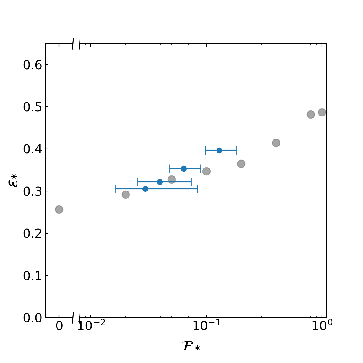
A.3 Effect on Star Formation Efficiency

We perform a set of numerical simulations by adopting Equation (A4) with fixed $\mathcal{F}_{*}$ for the grid-scale escape fraction of individual sink particles. We consider the fiducial cloud ($M_{\rm 0}=10^{5}\,M_{\odot}$ and $R_{\rm 0}=20\,{\rm pc}$) with radiation pressure feedback only (no photoionization). Figure 13 plots as gray circles the net SFE from the models with various $\mathcal{F}_{*}$. The net SFE increases mildly from 0.26 to 0.49 as $\mathcal{F}_{*}$ varies from 0 to 1. This is because as the feedback efficiency decreases (with increasing $\mathcal{F}_{*}$), more stellar mass is required to drive outflows to disrupt the cloud. We find that the timescales for star formation and cloud destruction do not vary by more than 10% in all runs with differing $\mathcal{F}_{*}$.

Figure 14: Cloud-scale reduction factor $\mathcal{F}$ for non-ionizing radiation as measured from the stellar center of luminosity as a function of $\langle\tau_{\rm n}^{\rm c}\rangle_{\Omega}$. The circles are from our simulations, with colors corresponding to $\sigma^{\rm c}$. The lines draw the reduction factor expected for lognormal PDFs with $\sigma^{\rm c}=0.5,1,\cdots,3.0$ from top to bottom.

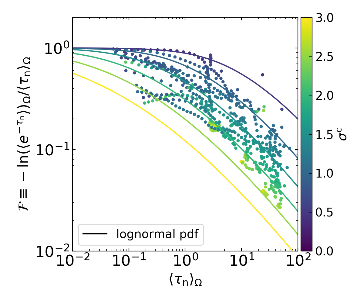
We also consider models in which $\mathcal{F}_{*}$ varies over time consistently with the instantaneous sink luminosity and accretion rate. While we cannot directly determine $\mathcal{F}_{*}$ without running simulations that resolve structures close to $r_{\rm s}$, the cloud-scale reduction factor $\mathcal{F}$ based on the resolved radiation-gas interaction (Section 4.1) can shed some light on the possible behavior of $\mathcal{F}_{*}$ at subgrid scales. Figure 7(b) showed that $\mathcal{F}$ tends to decrease with the width $\sigma_{c}$ of the optical-depth PDF and the solid angle-averaged optical depth $\langle\tau^{\rm c}\rangle_{\Omega}$. Figure 14 plots $\mathcal{F}$ again, this time as a function of $\langle\tau^{\rm c}\rangle_{\Omega}$. Most of the simulation results (filled circles) are consistent with the predictions of lognormal PDFs (lines) with $1.0\lesssim\sigma^{\rm c}\lesssim 2.5$. In the absence of photoionization and other feedback processes, one may assume that the accreting flows remain clumpy at subgrid scales and the reduction factor $\mathcal{F}_{*}$ is correlated with the angle-averaged optical depth of the accreting flow $\langle\tau_{\rm s}\rangle_{\Omega}$ in the same way that $\mathcal{F}$ is correlated with $\langle\tau^{\rm c}\rangle_{\Omega}$ as displayed in Figure 14.

Figure 15: 2D histograms of the grid-scale escape fraction $f_{\rm esc,*}$ and the mass accretion rate $\dot{M}_{*}$ onto sink particles for the fiducial cloud model, under the assumption that the optical-depth PDF at subgrid scales follows a lognormal distribution with the mean $\langle\ln\tau_{\rm s}\rangle_{\Omega}=\ln(\langle\tau_{\rm s}\rangle_{\Omega})+(\sigma^{\rm c})^{2}/2$ and the standard deviation $\sigma^{\rm c}=1.0,2.0,2.0,2.5$. The vertical solid lines mark the critical mass accretion rate $\dot{M}_{\rm*,crit,sph}$ for the existence of steady spherical inflow solutions (Krumholz, 2018). The thick dashed lines draw the relationship between $\dot{M}_{*}$ and $f_{\rm esc,*}$ expected for a cluster particle with mass $M_{*}=10^{3}\,M_{\odot}$ and a constant light-to-mass ratio $\Psi=10^{3}\,L_{\odot}\,M_{\odot}^{-1}$, while the thin dotted lines correspond to the case of the spherical accretion with $\mathcal{F}_{*}=1$.

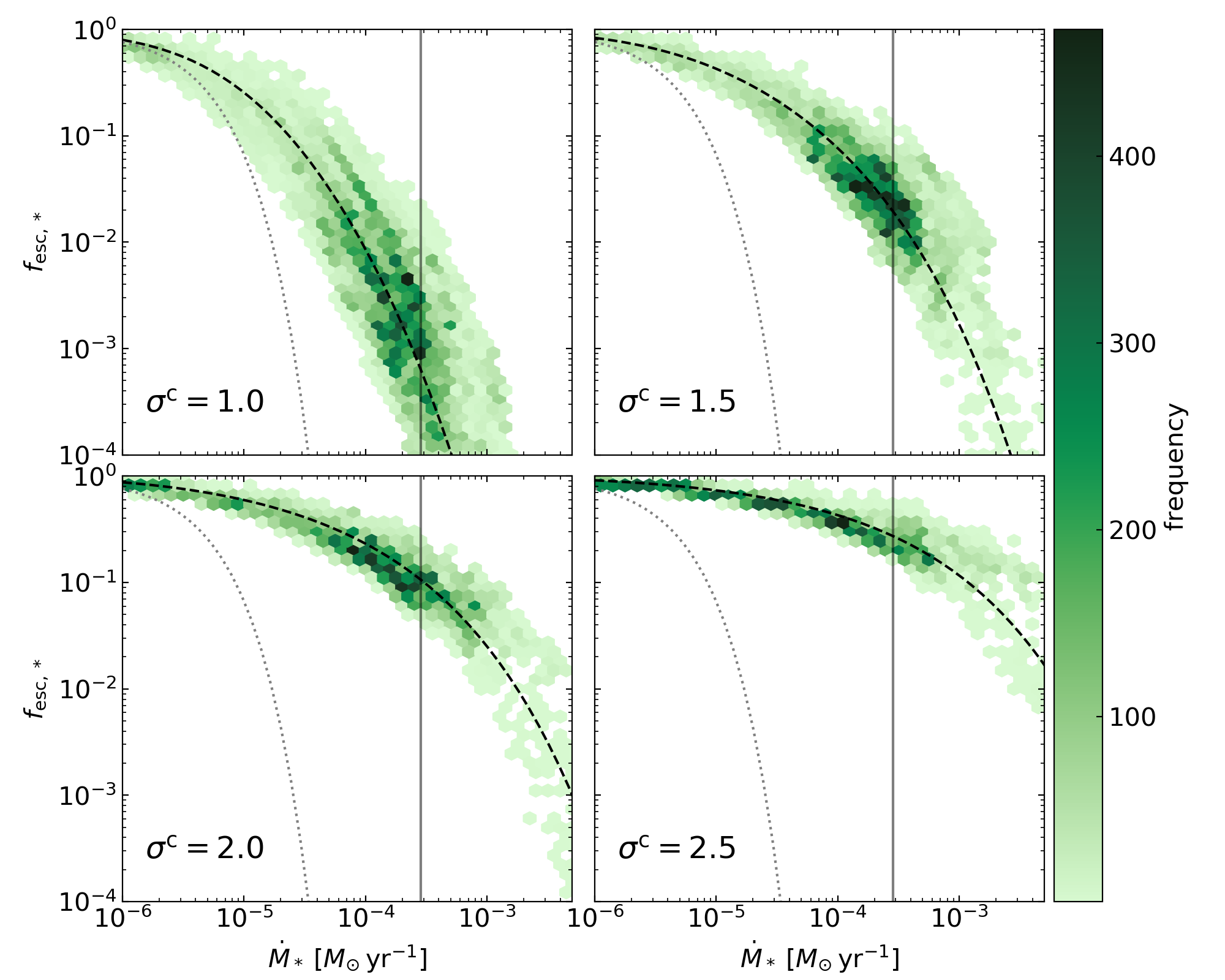
We run four simulations assuming that the optical-depth PDF on subgrid scales follows a lognormal distribution with $\sigma^{\rm c}=1.0$, $1.5$, $2.0$, and $2.5$. In each run with given $\sigma^{\rm c}$, we calculate $\langle\tau_{\rm s}\rangle_{\Omega}$ for individual sink particles using Equation (A1), obtain $\mathcal{F}_{*}$ from $\langle\tau_{\rm s}\rangle_{\Omega}$ using the corresponding $\mathcal{F}$–$\langle\tau^{\rm c}\rangle_{\Omega}$ relation shown as solid lines in Figure 14, and then apply the instantaneous escape fraction according to Equation (A4).

Figure 15 plots the 2D histograms on the $f_{\rm esc,*}$–$\dot{M}_{*}$ plane of sink particles in all runs. For reference, the thick dashed curves plot the relationships between $\dot{M}_{*}$ and $f_{\rm esc,*}$ expected for a cluster particle with mass $M_{*}=10^{3}\,M_{\odot}$ and light-to-mass ratio $\Psi=10^{3}\,L_{\odot}\,M_{\odot}^{-1}$ from Equations (A1)–(A4). Even when $\mathcal{F}_{*}$ is allowed to vary with $\langle\tau_{\rm s}\rangle_{\Omega}$, the escape fraction still decreases with increasing $\dot{M}_{*}$, but much more mildly compared to the case of spherical accretion with $\mathcal{F}_{*}=1$, plotted as thin dotted lines. When $\sigma^{\rm c}=2.0$, for example, the grid scale escape fraction $f_{\rm esc,*}$ drops below $\sim 10\%$ if $\dot{M}_{*}\gtrsim\dot{M}_{\rm*,crit,sph}=2.8\times 10^{-4}\,M_{\odot}\,{\rm yr}^{-1}(M_{*}/10^{3}\,M_{\odot})^{3/4}$. However, the mass accretion phase with $\dot{M}_{*}>\dot{M}_{\rm*,crit,sph}$ and $f_{\rm esc,*}\ll 1$ lasts only for a brief period of time ($\lesssim 1\,{\rm Myr}$), so that the evolution of cloud-scale escape fraction is not significantly affected by the choice of $\sigma^{\rm c}$. The median values of $\mathcal{F}_{*}$ for $10^{-6}\,M_{\odot}\,{\rm yr}^{-1}<\dot{M}_{*}<10^{-2}\,M_{\odot}\,{\rm yr}^{-1}$ in the four runs with $\sigma^{\rm c}=(1.0,1.5,2.0,2.5)$ are (0.13, 0.063, 0.039, 0.029), respectively. The resulting relationship between the net SFE and the subgrid-scale escape fraction from all four runs is plotted in Figure 13 as blue circles with horizontal bars, which is overall similar to the results with fixed $\mathcal{F}_{*}$.

To conclude, our numerical experiments demonstrate that the grid-scale escape fraction has a modest impact on the effectiveness of radiation feedback in halting accretion and controlling the SFE. To better understand the detailed process of gas-radiation interactions and provide constraints on $\mathcal{F}_{*}$ on smaller scales, it is desirable to perform numerical simulations of accretion flows onto massive stars resolving a wide range of spatial scales in the presence of various feedback mechanisms.

Figure 16: Effect of dust destruction in ionized gas for the fiducial cloud with $M_{\rm 0}=10^{5}\,M_{\odot}$ and $R_{\rm 0}=20\,{\rm pc}$. Time evolution of (a) total gas mass in the simulation domain (black), stellar mass (green), ejected gas mass (red), and photoevaporated gas mass (yellow); (b) instantaneous and (c) cumulative escape fractions for ionizing (orange) and non-ionizing (blue) radiation. The solid lines show the standard model (“No dest”) in which dust absorption cross section $\sigma_{\rm d}$ is constant everywhere ($1.17\times 10^{-21}{\rm cm}^{2}\,{\rm H}^{-1}$). The dashed lines show the comparison run in which destruction of dust grains in ionized gas is assumed to prevent absorption of ionizing radiation (Dest-i), while the dotted lines show the comparison run in which destruction of dust grains in ionized gas is assumed to prevent absorption of both non-ionizing and ionizing radiation (Dest-i/n). The vertical dashed line incidates the epoch of the first supernova ($t^{\prime}=3\,{\rm Myr}$).

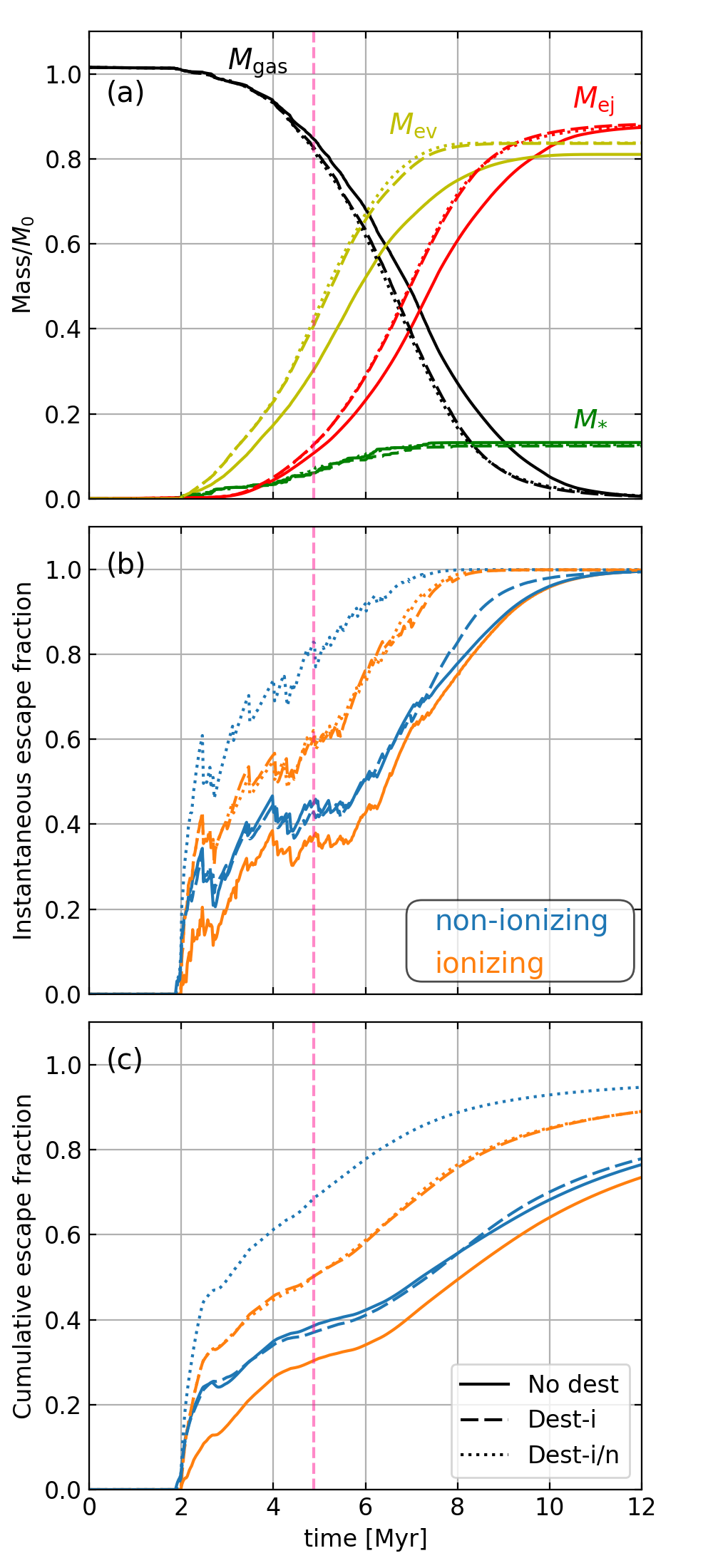
Appendix B Effects of Dust Destruction for the Fiducial Model

Our simulations adopted a constant grain absorption cross section $\sigma_{\rm d,i}=\sigma_{\rm d,n}=1.17\times 10^{-21}{\rm cm}^{2}\,{\rm H}^{-1}$ for both ionizing and non-ionizing radiation. For dust models characteristic of the diffuse ISM (e.g., Weingartner, & Draine, 2001), the UV extinction steeply rises toward shorter wavelengths and peaks at $h\nu\sim 17{\,{\rm eV}}$ due mainly to small carbon grains and PAHs (Draine, 2003; Glatzle et al., 2019); the frequency-averaged dust absorption cross section for ionizing radiation is $\sim(1$–$1.5)\times 10^{-21}\,{\rm cm}^{2}\,{\rm H}^{-1}$ for ionizing stars with blackbody temperature $2.5\times 10^{4}\,{\rm K}<T_{*}<5.0\times 10^{4}\,{\rm K}$ and has a slightly lower ($\sim 20$–$30\%$) value at FUV wavelengths (Draine, 2011). However, both theory and observations suggest that dust grains are destroyed by intense UV radiation in star-forming clouds (e.g., Voit, 1992; Tielens, 2008; Deharveng et al., 2010; Lopez et al., 2014; Salgado et al., 2016; Binder & Povich, 2018; Chastenet et al., 2019), which may lessen the UV extinction and boost escape of radiation in ionized gas. For example, Glatzle et al. (2019) adopted Weingartner, & Draine (2001)’s case A size distributions and found that $\sigma_{\rm d,i}$ can be reduced by a factor $\sim 2$–3 if the two log-normal components representing PAHs and very small carbon grains ($b_{\rm C}=0.0$) are completely absent.

To examine the potential impact of dust destruction on the escape of radiation, we have run additional simulations for the fiducial model ($M_{\rm 0}=10^{5}\,M_{\odot}$, $R_{\rm 0}=20\,{\rm pc}$, $N=256$) assuming that dust grains are destroyed in ionized gas. Since dust properties in H II regions are quite uncertain, we consider two extreme situations to bracket the range of possible outcomes:

• model Dest-i: the dust absorption cross section for ionizing radiation scales with the neutral fraction ($\sigma_{\rm d,i}=x_{\rm n}\times 1.17\times 10^{-21}{\rm cm}^{2}\,{\rm H}^{-1}$), but the cross section for non-ionizing radiation remains unchanged.

• model Dest-i/n: the dust absorption cross section for both ionizing and non-ionizing radiation scales with the neutral fraction ($\sigma_{\rm d,i}=\sigma_{\rm d,n}=x_{\rm n}\times 1.17\times 10^{-21}{\rm cm}^{2}\,{\rm H}^{-1}$).

The first of these corresponds to the preferential destruction of grains that absorb ionizing radiation in ionized gas, and the second corresponds to destruction of all grains in ionized gas. A similar approach has been adopted by Laursen et al. (2009), Howard et al. (2017), and Kimm et al. (2019). Since the complete destruction of dust grains in H II regions is unlikely to occur in reality, these models put an upper limit on the escape of radiation in H II regions.

Figure 16(a) plots the temporal evolution of gas mass ($M_{\rm gas}$, black), stellar mass ($M_{*}$, green), ejected gas mass ($M_{\rm ej}$, red), and photoevaporated gas mass ($M_{\rm ev}$, yellow) for different models. In the absence of dust grains to absorb ionizing photons in H II regions ($f_{\rm dust,i}\approx 0$), we expect photoionization feedback to be more efficient and the outflow driving by radiation pressure to be less efficient or absent (e.g., radiation pressure exerts no force on ionized gas in model Dest-i/n). As photoionization is the dominant feedback mechanism in low surface-density clouds (Paper II), it has a greater impact on the simulation outcome than radiation pressure. However, the overall cloud evolution does not change much. Compared to the standard model, the photoevaporation efficiency ($M_{\rm ev,final}/M_{\rm 0}$) is only 0.03 higher, while the net SFE is lower by less than 0.01 in both models Dest-i and Dest-i/n.

In contrast, the evolution of the escape of radiation is noticeably different from the standard model. Figure 16(b) and (c) show the evolution of instantaneous and cumulative escape fractions for ionizing (orange) and non-ionizing (blue) radiation. At $t^{\prime}=3\,{\rm Myr}$, the instantaneous escape fractions are $(f_{\rm esc,i},f_{\rm esc,n})=(0.60,0.42)$ in model Dest-i and $(f_{\rm esc,i},f_{\rm esc,n})=(0.62,0.83)$ in model Dest-i/n, while the cumulative escape fractions are $(f_{\rm esc,i}^{\rm cum},f_{\rm esc,n}^{\rm cum})=(0.50,0.37)$ in model Dest-i and $(f_{\rm esc,i}^{\rm cum},f_{\rm esc,n}^{\rm cum})=(0.50,0.69)$ in model Dest-i/n. In model Dest-i, $f_{\rm esc,n}$ and $f_{\rm esc,n}^{\rm cum}$ evolve quite similarly to those in the standard model, but are smaller than $f_{\rm esc,i}$ and $f_{\rm esc,i}^{\rm cum}$. In both models Dest-i and Dest-i/n, $f_{\rm esc,i}^{\rm cum}$ at $t^{\prime}=3\,{\rm Myr}$ is 0.20 greater than that in the standard run ($f_{\rm esc,i}^{\rm cum}=0.30$). In the standard model, ionizing photons escape through low-density density-bounded sightlines along which absorption by neutral hydrogen is unimportant and the escape fraction is mainly determined by dust absorption (Section 3.2). Therefore, the escape fraction $f_{\rm esc,i}$ in the absence of dust absorption simply reflects (the luminosity-weighted average of) the fraction of the sightlines that are density-bounded.

References

- Abel & Wandelt (2002) Abel, T., & Wandelt, B. D. 2002, MNRAS, 330, L53
- Bertoldi & McKee (1992) Bertoldi, F., & McKee, C. F. 1992, ApJ, 395, 140
- Binder & Povich (2018) Binder, B. A., & Povich, M. S. 2018, ApJ, 864, 136
- Borthakur et al. (2014) Borthakur, S., Heckman, T. M., Leitherer, C., & Overzier, R. A. 2014, Science, 346, 216
- Bouwens et al. (2011) Bouwens, R. J., Illingworth, G. D., Oesch, P. A., et al. 2011, ApJ, 737, 90
- Bromm & Yoshida (2011) Bromm, V., & Yoshida, N. 2011, ARA&A, 49, 373
- Burkhart & Lazarian (2012) Burkhart, B., & Lazarian, A. 2012, ApJ, 755, L19.
- Chastenet et al. (2019) Chastenet, J., Sandstrom, K., Chiang, I.-D., et al. 2019, ApJ, 876, 62
- Dale (2015) Dale, J. E. 2015, New A Rev., 68, 1
- Dale et al. (2013) Dale, J. E., Ercolano, B., & Bonnell, I. A. 2013, MNRAS, 430, 234
- Dale et al. (2012) Dale, J. E., Ercolano, B., & Bonnell, I. A. 2012, MNRAS, 424, 377
- Domgorgen & Mathis (1994) Domgorgen, H., & Mathis, J. S. 1994, ApJ, 428, 647
- Dopita et al. (2003) Dopita, M. A., Groves, B. A., Sutherland, R. S., & Kewley, L. J. 2003, ApJ, 583, 727
- Doran et al. (2013) Doran, E. I., Crowther, P. A., de Koter, A., et al. 2013, A&A, 558, A134
- Dove et al. (2000) Dove, J. B., Shull, J. M., & Ferrara, A. 2000, ApJ, 531, 846
- Draine (2003) Draine, B. T. 2003, ARA&A, 41, 241
- Draine (2011) Draine, B. T. 2011, ApJ, 732, 100
- Ferguson et al. (1996) Ferguson, A. M. N., Wyse, R. F. G., Gallagher, J. S., III, & Hunter, D. A. 1996, AJ, 111, 2265
- Finkelstein et al. (2019) Finkelstein, S. L., D’Aloisio, A., Paardekooper, J.-P., et al. 2019, ApJ, 879, 36
- Finkelstein et al. (2012) Finkelstein, S. L., Papovich, C., Ryan, R. E., et al. 2012, ApJ, 758, 93
- Geen et al. (2015) Geen, S., Rosdahl, J., Blaizot, J., Devriendt, J., & Slyz, A. 2015, MNRAS, 448, 3248
- Geen et al. (2017) Geen, S., Soler, J. D., & Hennebelle, P. 2017, MNRAS, 471, 4844
- Glatzle et al. (2019) Glatzle, M., Ciardi, B., & Graziani, L. 2019, MNRAS, 482, 321
- Górski et al. (2005) Górski, K. M., Hivon, E., Banday, A. J., et al. 2005, ApJ, 622, 759
- Gong & Ostriker (2013) Gong, H., & Ostriker, E. C. 2013, ApJS, 204, 8
- Goodman et al. (2009) Goodman, A. A., Pineda, J. E., & Schnee, S. L. 2009, ApJ, 692, 91
- Grudić et al. (2018) Grudić, M. Y., Hopkins, P. F., Faucher-Giguère, C.-A., et al. 2018, MNRAS, 475, 3511
- Haffner et al. (2009) Haffner, L. M., Dettmar, R.-J., Beckman, J. E., et al. 2009, Reviews of Modern Physics, 81, 969
- Heckman et al. (2011) Heckman, T. M., Borthakur, S., Overzier, R., et al. 2011, ApJ, 730, 5
- Hoare et al. (2007) Hoare, M. G., Kurtz, S. E., Lizano, S., Keto, E., & Hofner, P. 2007, Protostars and Planets V, 181
- Hollenbach & Tielens (1999) Hollenbach, D. J., & Tielens, A. G. G. M. 1999, Reviews of Modern Physics, 71, 173
- Hoopes et al. (1996) Hoopes, C. G., Walterbos, R. A. M., & Greenwalt, B. E. 1996, AJ, 112, 1429
- Hopkins & Grudić (2019) Hopkins, P. F., & Grudić, M. Y. 2019, MNRAS, 483, 4187
- Hunter (2007) Hunter, J. D. 2007, CSE, 9, 90
- Howard et al. (2017) Howard, C., Pudritz, R., & Klessen, R. 2017, ApJ, 834, 40
- Howard et al. (2018) Howard, C. S., Pudritz, R. E., Harris, W. E., & Klessen, R. S. 2018, MNRAS, 475, 3121
- Iffrig & Hennebelle (2015) Iffrig, O., & Hennebelle, P. 2015, A&A, 576, A95
- Inoue (2002) Inoue, A. K. 2002, ApJ, 570, L97
- Inoue et al. (2001) Inoue, A. K., Hirashita, H., & Kamaya, H. 2001, ApJ, 555, 613
- Izotov et al. (2016) Izotov, Y. I., Schaerer, D., Thuan, T. X., et al. 2016, MNRAS, 461, 3683
- Izotov et al. (2018) Izotov, Y. I., Schaerer, D., Worseck, G., et al. 2018, MNRAS, 474, 4514
- Kainulainen et al. (2009) Kainulainen, J., Beuther, H., Henning, T., & Plume, R. 2009, A&A, 508, L35
- Kakiichi, & Gronke (2019) Kakiichi, K., & Gronke, M. 2019, arXiv e-prints, arXiv:1905.02480
- Kennicutt & Evans (2012) Kennicutt, R. C., & Evans, N. J. 2012, ARA&A, 50, 531
- Kim et al. (2013) Kim, C.-G., Ostriker, E. C., & Kim, W.-T. 2013, ApJ, 776, 1
- Kim et al. (2017) Kim, C.-G., Ostriker, E. C., & Raileanu, R. 2017, ApJ, 834, 25
- Kim & Ostriker (2017) Kim, C.-G., & Ostriker, E. C. 2017, ApJ, 846, 133
- Kim et al. (2016) Kim, J.-G., Kim, W.-T., & Ostriker, E. C. 2016, ApJ, 819, 137
- Kim et al. (2018) Kim, J.-G., Kim, W.-T., & Ostriker, E. C. 2018, ApJ, 859, 68 (Paper II)
- Kim et al. (2017) Kim, J.-G., Kim, W.-T., Ostriker, E. C., & Skinner, M. A. 2017, ApJ, 851, 93 (Paper I)
- Kim & Koo (2003) Kim, K.-T., & Koo, B.-C. 2003, ApJ, 596, 362
- Kim & Koo (2001) Kim, K.-T., & Koo, B.-C. 2001, ApJ, 549, 979
- Kimm, & Cen (2014) Kimm, T., & Cen, R. 2014, ApJ, 788, 121
- Kimm et al. (2017) Kimm, T., Katz, H., Haehnelt, M., et al. 2017, MNRAS, 466, 4826
- Kimm et al. (2019) Kimm, T., Blaizot, J., Garel, T., et al. 2019, MNRAS, 486, 2215
- Kreckel et al. (2016) Kreckel, K., Blanc, G. A., Schinnerer, E., et al. 2016, ApJ, 827, 103
- Krumholz et al. (2007) Krumholz, M. R., Stone, J. M., & Gardiner, T. A. 2007, ApJ, 671, 518
- Krumholz et al. (2014) Krumholz, M. R., Bate, M. R., Arce, H. G., et al. 2014, Protostars and Planets VI, 243
- Krumholz (2018) Krumholz, M. R. 2018, MNRAS, 480, 3468
- Krumholz et al. (2018) Krumholz, M. R., McKee, C. F., & Bland-Hawthorn, J. 2018, arXiv e-prints , arXiv:1812.01615.
- Lacerda et al. (2018) Lacerda, E. A. D., Cid Fernandes, R., Couto, G. S., et al. 2018, MNRAS, 474, 3727
- Laursen et al. (2009) Laursen, P., Sommer-Larsen, J., & Andersen, A. C. 2009, ApJ, 704, 1640
- Lefloch & Lazareff (1994) Lefloch, B., & Lazareff, B. 1994, A&A, 289, 559
- Leitet et al. (2013) Leitet, E., Bergvall, N., Hayes, M., Linné, S., & Zackrisson, E. 2013, A&A, 553, A106
- Leitherer et al. (2016) Leitherer, C., Hernandez, S., Lee, J. C., & Oey, M. S. 2016, ApJ, 823, 64
- Loeb & Barkana (2001) Loeb, A., & Barkana, R. 2001, ARA&A, 39, 19
- Lombardi et al. (2014) Lombardi, M., Bouy, H., Alves, J., & Lada, C. J. 2014, A&A, 566, A45
- Lopez et al. (2014) Lopez, L. A., Krumholz, M. R., Bolatto, A. D., et al. 2014, ApJ, 795, 121
- Ma et al. (2015) Ma, X., Kasen, D., Hopkins, P. F., et al. 2015, MNRAS, 453, 960
- Mathis (2000) Mathis, J. S. 2000, ApJ, 544, 347
- McCandliss et al. (2019) McCandliss, S., Calzetti, D., Ferguson, H. C., et al. 2019, BAAS, 51, 535
- McLeod et al. (2019) McLeod, A. F., Dale, J. E., Evans, C. J., et al. 2019, MNRAS, 486, 5263
- McKee & Ostriker (2007) McKee, C. F., & Ostriker, E. C. 2007, ARA&A, 45, 565
- McKinney (2010) McKinney, W. 2010, in Proc. 9th Python in Science Conf., Data Structures for Statistical Computing in Python, ed. S. van der Walt & J. Millman (Austin, TX: SciPy), 51
- Oey et al. (2007) Oey, M. S., Meurer, G. R., Yelda, S., et al. 2007, ApJ, 661, 801
- Ostriker et al. (2010) Ostriker, E. C., McKee, C. F., & Leroy, A. K. 2010, ApJ, 721, 975
- Paardekooper et al. (2015) Paardekooper, J.-P., Khochfar, S., & Dalla Vecchia, C. 2015, MNRAS, 451, 2544
- Parravano et al. (2003) Parravano, A., Hollenbach, D. J., & McKee, C. F. 2003, ApJ, 584, 797
- Pellegrini et al. (2012) Pellegrini, E. W., Oey, M. S., Winkler, P. F., et al. 2012, ApJ, 755, 40
- Pérez & Granger (2007) Pérez, F., & Granger, B. E. 2007, CSE, 9, 21
- Petrosian et al. (1972) Petrosian, V., Silk, J., & Field, G. B. 1972, ApJ, 177, L69
- Poetrodjojo et al. (2019) Poetrodjojo, H., D’Agostino, J. J., Groves, B., et al. 2019, MNRAS, 1197.
- Rahner et al. (2017) Rahner, D., Pellegrini, E. W., Glover, S. C. O., et al. 2017, MNRAS, 470, 4453
- Raskutti et al. (2016) Raskutti, S., Ostriker, E. C., & Skinner, M. A. 2016, ApJ, 829, 130
- Raskutti et al. (2017) Raskutti, S., Ostriker, E. C., & Skinner, M. A. 2017, ApJ, 850, 112
- Reynolds (1984) Reynolds, R. J. 1984, ApJ, 282, 191
- Rigby et al. (2019) Rigby, J., Berg, D., Bordoloi, R., et al. 2019, BAAS, 51, 245
- Rivera-Thorsen et al. (2019) Rivera-Thorsen, T. E., Dahle, H., Chisholm, J., et al. 2019, arXiv:1904.08186
- Robertson et al. (2010) Robertson, B. E., Ellis, R. S., Dunlop, J. S., McLure, R. J., & Stark, D. P. 2010, Nature, 468, 49
- Robertson et al. (2015) Robertson, B. E., Ellis, R. S., Furlanetto, S. R., & Dunlop, J. S. 2015, ApJ, 802, L19
- Rogers & Pittard (2013) Rogers, H., & Pittard, J. M. 2013, MNRAS, 431, 1337
- Rosdahl et al. (2015) Rosdahl, J., Schaye, J., Teyssier, R., et al. 2015, MNRAS, 451, 34
- Salgado et al. (2016) Salgado, F., Berné, O., Adams, J. D., et al. 2016, ApJ, 830, 118
- Sembach et al. (2000) Sembach, K. R., Howk, J. C., Ryans, R. S. I., & Keenan, F. P. 2000, ApJ, 528, 310
- Shapley et al. (2016) Shapley, A. E., Steidel, C. C., Strom, A. L., et al. 2016, ApJ, 826, L24
- Skinner & Ostriker (2015) Skinner, M. A., & Ostriker, E. C. 2015, ApJ, 809, 187
- Smith (2006) Smith, N. 2006, MNRAS, 367, 763
- Smith & Brooks (2007) Smith, N., & Brooks, K. J. 2007, MNRAS, 379, 1279
- Stone & Gardiner (2009) Stone, J. M., & Gardiner, T. 2009, New A, 14, 139
- Stone et al. (2008) Stone, J. M., Gardiner, T. A., Teuben, P., Hawley, J. F., & Simon, J. B. 2008, ApJS, 178, 137
- Tan et al. (2014) Tan, J. C., Beltrán, M. T., Caselli, P., et al. 2014, Protostars and Planets VI, 149
- Tielens (2008) Tielens, A. G. G. M. 2008, ARA&A, 46, 289
- Trebitsch et al. (2017) Trebitsch, M., Blaizot, J., Rosdahl, J., Devriendt, J., & Slyz, A. 2017, MNRAS, 470, 224
- Tsang & Milosavljević (2018) Tsang, B. T.-H., & Milosavljević, M. 2018, MNRAS, 478, 4142
- Turk et al. (2011) Turk, M. J., Smith, B. D., Oishi, J. S., et al. 2011, ApJS, 192, 9
- van der Walt et al. (2011) van der Walt, S., Colbert, S. C., & Varoquaux, G. 2011, CSE, 13, 22
- Voges et al. (2008) Voges, E. S., Oey, M. S., Walterbos, R. A. M., & Wilkinson, T. M. 2008, AJ, 135, 1291
- Voit (1992) Voit, G. M. 1992, MNRAS, 258, 841
- Walch et al. (2012) Walch, S. K., Whitworth, A. P., Bisbas, T., Wünsch, R., & Hubber, D. 2012, MNRAS, 427, 625
- Weilbacher et al. (2018) Weilbacher, P. M., Monreal-Ibero, A., Verhamme, A., et al. 2018, A&A, 611, A95
- Weingartner, & Draine (2001) Weingartner, J. C., & Draine, B. T. 2001, ApJ, 548, 296
- Wise et al. (2014) Wise, J. H., Demchenko, V. G., Halicek, M. T., et al. 2014, MNRAS, 442, 2560
- Wise (2019) Wise, J. H. 2019, arXiv e-prints, arXiv:1907.06653
- Wolfire et al. (1995) Wolfire, M. G., Hollenbach, D., McKee, C. F., Tielens, A. G. G. M., & Bakes, E. L. O. 1995, ApJ, 443, 152
- Wolfire et al. (2003) Wolfire, M. G., McKee, C. F., Hollenbach, D., & Tielens, A. G. G. M. 2003, ApJ, 587, 278
- Deharveng et al. (2010) Deharveng, L., Schuller, F., Anderson, L. D., et al. 2010, A&A, 523, A6
- Zurita et al. (2000) Zurita, A., Rozas, M., & Beckman, J. E. 2000, A&A, 363, 9