Galactic Cosmic Ray Sun Shadow during the declining phase of cycle 24 observed by HAWC

Abstract:

The High Altitude Water Cherenkov (HAWC) array is sensitive to high energy Cosmic Rays (CR) in the $\sim 10$ to $\sim 200$ TeV energy range, making it possible to construct maps of the so called “Sun Shadow” ($SS$), i. e. of the deficit of CR coming from the direction of the Sun. In this work, we present the variation of the Relative Intensity of the deficit ($SS_{RI}$) for three years of HAWC observations form 2016 to 2018 in which we found a clear decreasing trend of the ($SS_{RI}$) over the studied period, corresponding to the declining phase of the solar cycle 24. By comparing the $SS_{RI}$ with the photospheric magnetic field evolution, we show that there is a linear relationship between the $SS_{RI}$ and the median photospheric magnetic field of the Active Region belt (-40${}^{\circ}\leq$ lat $\leq$ 40^∘) and a inverse linear relationship with the polar photospheric magnetic field (lat $\geq\pm$ 60^∘). The former relationship is due to the magnetic field causing a deviation of the CR, whereas the latter reflects the change of the heliospheric field topology from multipolar to dipolar configurations. These relationships are valid only when the median magnetic field is lower than 8 G, during the declining and minimum phases of the solar cycle 24. Finally, we show that relativistic charged particles, in the 10 to 200 TeV energy range, are deflected a few degrees.

1 Introduction

HAWC is an air shower array located at 4100 m above the sea level on the Sierra Negra Volcano in the central part of Mexico (N 18^∘ 59’ 48”, W 97^∘ 18’ 34”), intended for the exploration of the Northern hemisphere sky in high energy gamma rays. Although, as the majority of primary particles (¿ 99%) are hadrons, HAWC is a sensitive Galactic Cosmic Rays (GCR) telescope with an energy range from $\sim 10$ to $\sim 200$ TeV. A description of HAWC is presented in [1, 2].

GCRs are charged particles, mainly protons, with energies ranging form few $10^{6}$ up to $10^{20}$ eV arriving isotropically from outside the heliosphere. The heliospheric magnetic field modulates the GCR flux that reaches the Earth, making the study of GCR an excellent tool to remotely explore the Heliosphere. For example, low energy GCRs (E $<10^{6}$) provide information on the outer Heliospheric Magnetic Field [3] and long term solar modulation [4]. At higher energies (tens of GeV) GCRs are well suited for short term solar transient studies, such as coronal mass ejections, solar flares and high speed steamers [5]. Only high energy GCRs (E $>10^{12}$ eV) are unaffected by the interplanetary magnetic fields and therefore, are able to reach the low atmosphere of the Sun, interacting there with both: the strong near-photospheric magnetic fields and particles [6] giving in this way, valuable information of these fields. At the Earth, an observer with a sufficiently sensitive GCR telescope pointing towards the Sun, will see the deficit of the high energy GCR flux, because of the Sun’s physical presence and the deviation of the GCRs caused by the solar magnetic field.

In this work we use the High Altitude Water Cherenkov Array data to construct maps of the high energy GCR deficit observed at the solar position, the so called Sun Shadow ($SS$) maps (Sec. 2). Because HAWC has been observing the high energy sky since 2016, we have enough data to explore the SS with long integration times (giving signal to noise ratios greater than 40) and with medium integration times corresponding to one Carrington Rotation ($\sim 27$ days). The period of our study corresponds to the declining phase of Cycle 24 and in Sec. 3. We explore the photospheric magnetic field evolution during this phase. The physical connection between high energy GCR and the photospheric magnetic field is explored through a basic simulation in Sec. 4. Finally, our conclusions are in Sec. 5.

2 Sun Shadow Maps

We have used standard HAWC procedures [2, 7, 8] to construct sky maps in a region where the Sun is positioned and the GCR deficit or Sun Shadow is caused by the interaction between these GCR and both: the Sun itself and the magnetic field of the solar atmosphere [9]. For this work, we consider HAWC data taken during the years 2016 to 2018 and compute the $SS_{RI}$ maps integrated on a yearly basis, as shown in Figures 1 (a and b), and 2 (a), respectively.

(a) 2016

(b) 2017

Figure 1: Maps of the relative intensity of the $SS_{RI}$ integrated during 2016 (a) and 2017 (b) The contours correspond to the 2D fitted to each map.

It is clear that the $SS_{RI}$ changes with time. To order quantify these changes, we fitted a circular 2-dimensional gaussian $F(x,y)=A_{0}+A_{RI}\exp(-(((x-C_{x})/W_{x})^{2}+((y-C_{y})/W_{y})^{2})/2)$ where $W_{x}=W_{y}$. For example, Figure 2 (b) shows the 2D gaussian fitted to the $SS_{RI}$ map integrated for the year 2018. $A_{RI}$ corresponds to the relative intensity deficit measured by the height of the 2D gaussian and this is the parameter selected for the analysis in this work. The $A_{RI}$ distribution is plotted in Figure 3. The distributions of the widths and centroids of the fitted 2D gaussians are shown in Figure 4, where the dashed vertical lines mark the cuts in both parameters that we consider for further analysis. These are maps with $0.6\leq W\leq 1.3$ and $-0.5\leq C_{x,y}\leq 0.5$.

(a)

(b)

Figure 2: (a) Similar as Figure 1 but for the year 2018 and its fitted 2D gaussian (b).

As HAWC is located at $\sim 19^{\circ}$ North latitude, so the apparent latitudinal movement of the Sun with respect to the observatory zenith angle ($\theta_{z}$) changes during the year from +4.5^∘ to -42.5^∘, and taking into account that the observational limit of HAWC is $\sim 40^{\circ}$, this implies that during six months of the year (April to September) the $\theta_{z}$ is $<20^{\circ}$. We consider this to be the best time window for our study. Therefore, we limit our study to Carrington rotations within this time window. Furthermore, as the detected GCR flux decreases as $\sim\cos({\theta_{az}})$, for this work we assume that our uncertainty ($\epsilon$, marked by the error bars in the following Figures) is: $\epsilon=\sqrt{\epsilon_{RI}^{2}+A_{RI}\cos({\frac{9}{2}\theta_{az}+\pi})^{2}}$ where $A_{0}$ and $\epsilon_{fit}$ are the fitted amplitude and its associated error and the factor $\frac{9}{2}$ maximizes the error when $\theta_{z}=20^{\circ}$.

Figure 3: Distribution of the amplitudes of the gaussians fitted to the GCR deficit maps.

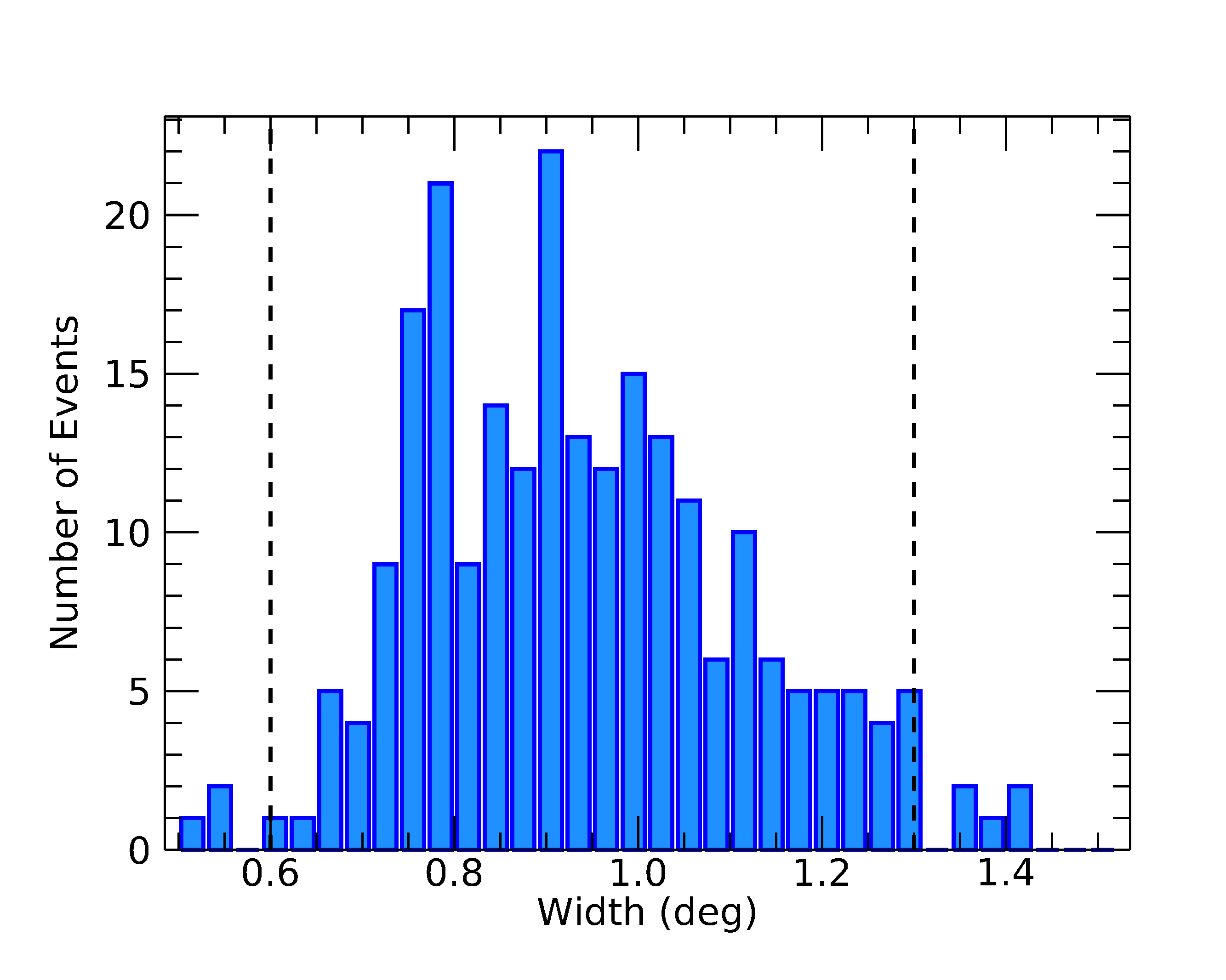
(a) 2016

(b) 2017

Figure 4: Distribution of the widths (a) and centroid (b) of the gaussians fitted to the GCR deficit maps.

2.1 Time Evolution

The relative intensity decreases over the time during our period of analysis as shown in Figure 5 (a) where we show the variation with time of the relative intensity maps integrated over one year. The high sensitivity of HAWC allows us to compute $SS_{RI}$ maps with relatively short integration times. In this work, we have generated maps with integration times of one solar rotation, i. e., we have computed a map for each Carrington Rotation (Carr_Rot) in our period of study, starting with Carr_Rot 2173 (Jan 21, 2016) up to Carr_Rot 2210 (Oct 26, 2018). Clearly, the time evolution of the $SS_{RI}$ integrated by Carr_Rot also decreases along the time as shown in Figure 5 (a) where the $A_{RI}$ during each Carr_Rot are plotted.

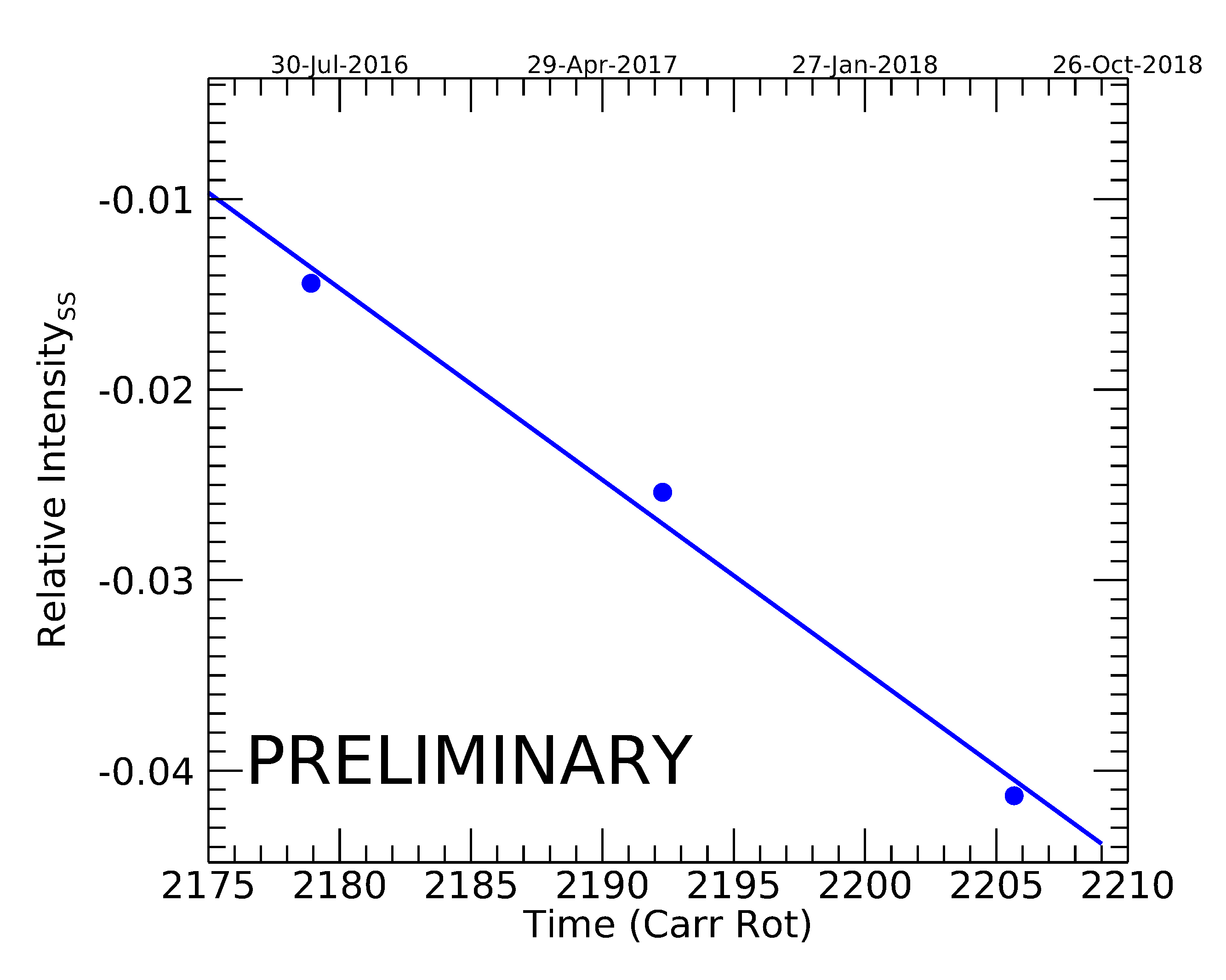
(a)

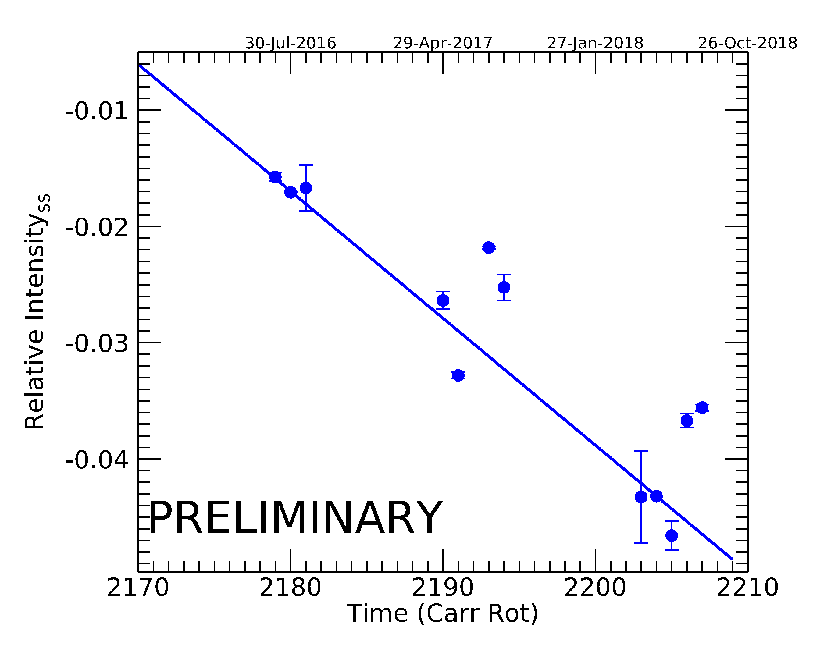
(b)

Figure 5: Relative Intensity of the $SS_{RI}$ as a function of time, integrated by six months (a) and one Carr_Rot (b).

Further more the dependence of the RI is quasi-linear with the time with a rate of change of -0.013 and -0.015 year^-1 for the yearly and Carr_Rot integrated maps, respectively.

It is well know that the GCR flux is modulated by the solar activity. Although this modulation has been observed at relatively low energies (up to several tens of GeV) and is attributed to the solar wind and the large scale disturbances traveling in it. At higher energies ($\sim 10-200$ TeV), as the HAWC maps analyzed in this work, the modulation should occur only very close to the solar surface where the magnetic field is strong enough to deviate such high energy particles.

3 Solar Cycle and Photospheric Magnetic Field

The solar activity follows a magnetic cycle of $\sim$ 22 years, and during the 2016-2018 period, the solar cycle 24 was declining as shown by the Sun Spot Number (SSN) plotted in Figure 6 (a). In similar way, the modulated CGR flux measured by neutron monitors changes during the cycle as shown in Figure 6 (b).

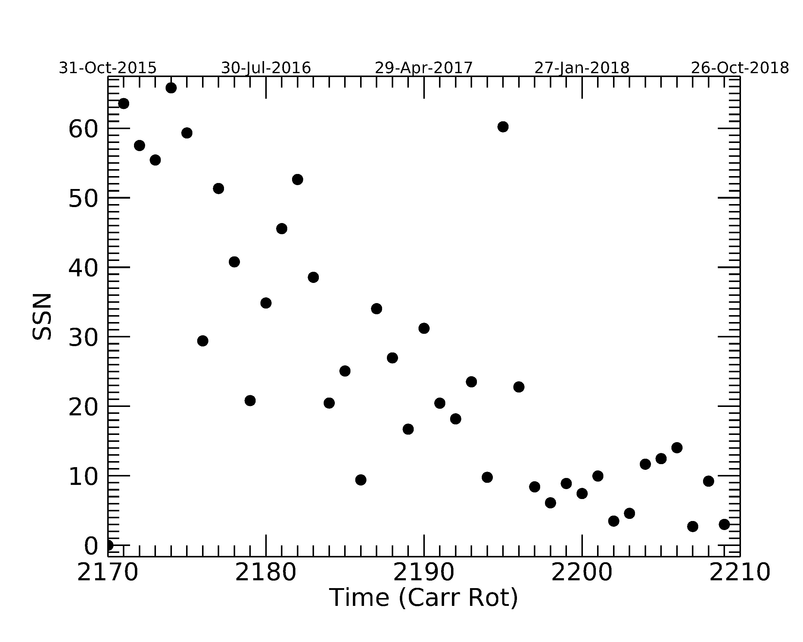
(a)

(b)

Figure 6: SSN during solar cycle 24 (a), and the modulated GCR flux as observed by Neutron Monitors during the same period (b).

The SSN is a proxy of the solar activity, and should not be compared directly with the GCR modulation, rather the magnetic field (and the solar wind speed for low energy GCR) should be used. This represents a problem for low energy GCR studies, due to the fact that our measurements of the solar wind parameters are limited to one or few points in the heliosphere, where spacecraft reside. Conversely, the high energy GCRs that HAWC observes are related to strong magnetic fields in the low solar atmosphere, which are measurable (in the case of the photosphere) and can be extrapolated up to few solar radii with a magnetic potential (current free) model.

In this work we compare the changes in the $SS_{RI}$ with the photospheric magnetic field. Because this field is highly variable, from $\sim 1000$ G inside Active Regions to $\sim 1$ 1 G in quiet regions, we use the median to characterize this field. Figure 7 (a) shows the evolution of the median photospheric magnetic field as a function of time during our period of study. To compare this evolution with that of the $SS_{RI}$, Figure 7 (b) shows the RI of the $SS_{RI}$ as a function of the median photospheric magnetic field.

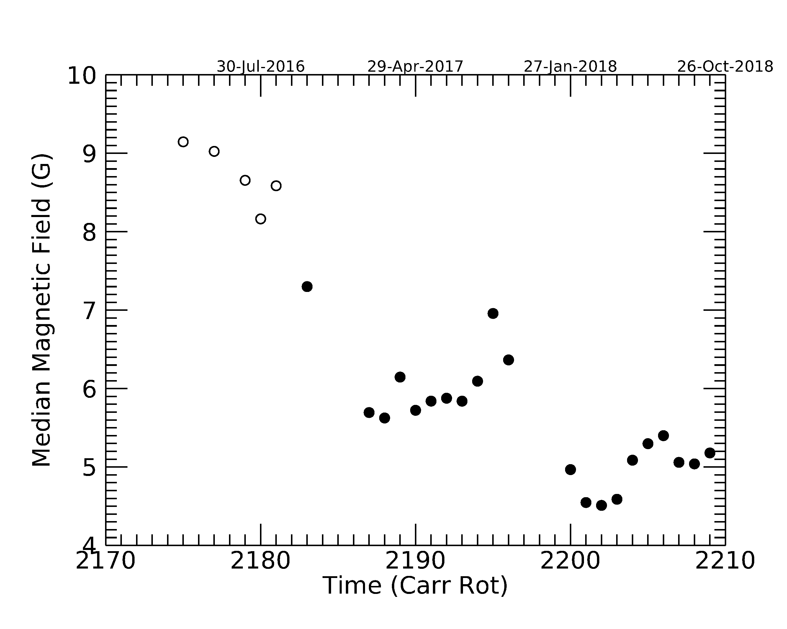
(a)

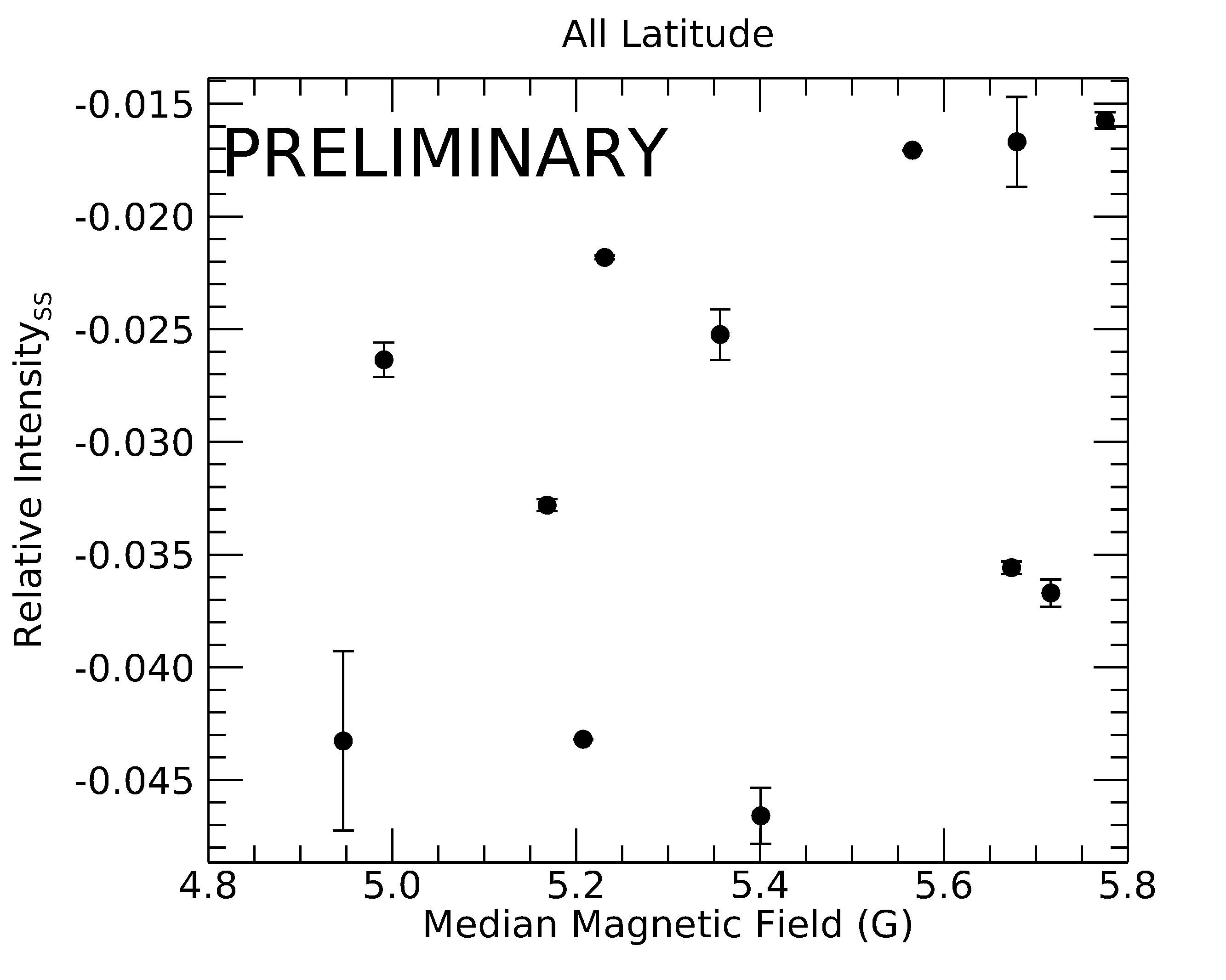
(b)

Figure 7: (a) Median photospheric magnetic field computed at all latitudes for each Carr_Rot considered in this work. (b) The $A_{RI}$ as a function of the median photospheric magnetic field.

We attribute this lack of correlation to the fact that the solar magnetic field evolves differently, depending on the latitude. For example, in the so called Active Region belt (ranging from $\sim-30^{\circ}$ to $\sim 30^{\circ}$ of latitude), the magnetic field attains the highest strengths during the maximum of activity with a toroidal configuration, wheras this strength is lowest during the minimum of activity. On the other hand the configuration on the poles (lat $\geq\pm 60^{\circ}$) attains the the lowest values during the maximum and increases towards the minimum of activity with a global dipolar topology.

The RI as a function of the toroidal (low latitudes) and poloidal (high latitudes) magnetic fields are shown in Figures 8 a and b, respectively.

(a)

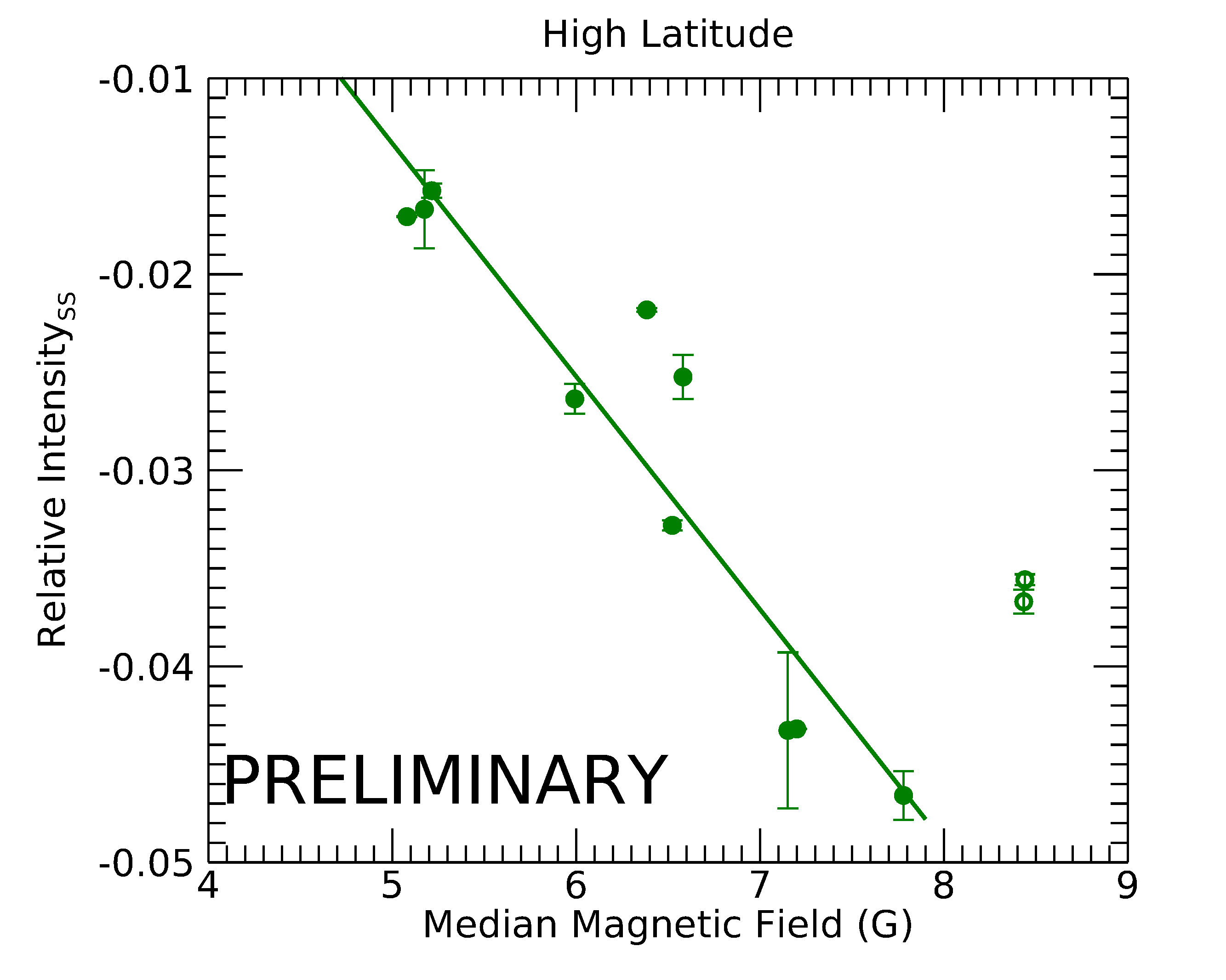
(b)

Figure 8: The $A_{RI}$ as a function of the median photospheric magnetic field at low (a) and high (b) latitudes.

Interestingly, the dependence (at low magnetic field values), of the RI with the magnetic field is linear at both low and high latitudes, but of opposite sign. The corresponding rates of change are $1.46\times 10^{-2}$ G^-1 and $-1.19\times 10^{-2}$ G^-1.

This relationship is valid for low activity periods, where the median magnetic field is lower than 8 G. When the solar activity and the magnetic field is greater, as during Carr_Rots 2179 , 2180 and 2181 (on July and August 2016) the linear relationship is no longer valid, as seen in Figure 8.

4 Bending of cosmic rays in coronal magnetic field

A simulation was performed to estimate the GCR bending in the solar corona. In this approximation, the solar magnetic field was modeled assuming a symmetric photospheric field ($B_{phot}$) with a range of 0.1 to 20 G and decreasing as the square of the radial distance ($B_{r}=\frac{B_{phot}}{(r-r_{phot})^{2}}$). The Larmor radius of a CR in the magnetic field is given as,

$$R_{L}~{}~{}=~{}~{}(3.3\times 10^{12}~{}cm)\times\frac{E(GeV)}{B(\mu G)}$$ (1)

The deviation experienced by the cosmic ray while it is traveling a small distance ’$dL$’ through the magnetic field can be expressed in terms of the Larmor radius as $d\Theta=dL/R_{L}$. The total deflection angle of the particle was estimated by a numerical integration over its trajectory within the magnetic field profile as described above. The simulation was carried out for different energies; tracing the trajectory of the particle inside the corona; defining the initial distance as the distance between the photosphere and the line marked by the initial trajectory of the particle along a radius perpendicular to this line; and setting the initial and final integration points the positions where the particle crosses the 3 $R_{\odot}$ limit. As an example, Figure 9 shows the deviation angle (indicated by the color code) as a function of the initial distance and the photospheric magnetic field for two energy bins of HAWC, 7 and 85 TeV on the left and right panels respectively. It is clear that the deviation angle is less than 2^∘ when particles of 7 and 85 TeV traverse the atmosphere at an initial distance of 2 and 0.3 solar radii, respectively.

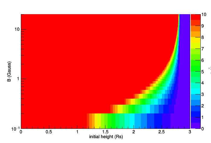
(a)

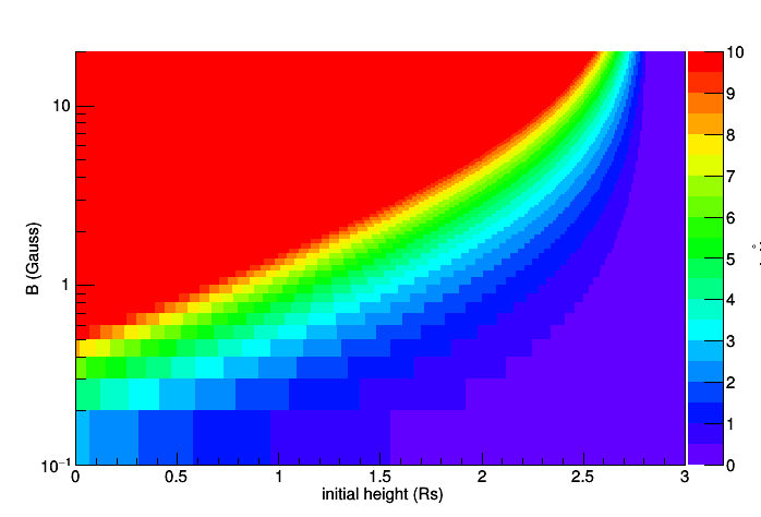
(b)

Figure 9: Simulations of the deviation of GCR of 7 (left) and 85 (right) TeV, passing through the coronal magnetic field.

5 Summary and Conclusions

We performed a temporal analysis of the deficit of GCR caused by the Sun during the 2016 to 2018 year period. In particular, we analyzed the behavior of the amplitude of a 2D symmetric gaussian, adjusted to the relative intensity maps of the $SS$ made using two integration times of $\sim 1$ and 6 months. We found a decreasing trend of the $SS_{RI}$ with time. Furthermore, by comparing the $SS_{RI}$ with the photospheric magnetic field, we found a linear correlation between the signal amplitude and the median magnetic field measured at the Active Region belt ($-30^{\circ}\geq$ Lat $\geq 30^{\circ}$), i.e., with the toroidal magnetic field during the high activity phase of the cycle, and a linear anti-correlation between the $SS_{RI}$ and the median magnetic field at polar regions ( Lat $\geq\pm 60^{\circ}$). This is related to the transition from a multipolar configuration to a simpler dipolar magnetic field during the low activity phase. Finally, we presented simulations of the passage of high energy particles through a spherical symmetrical magnetic field, to show that the GCR of energies detected by HAWC are deviated few degrees and cause the observed $SS$.

References

- [1] Abeysekara, A. U., and 104 colleagues 2014. Sensitivity of HAWC to high-mass dark matter annihilations. Physical Review D 190, 122002.
- [2] Abeysekara, A. U., and 106 colleagues 2017. Observation of the Crab Nebula with the HAWC Gamma-Ray Observatory. The Astrophysical Journal 843, 39.
- [3] Haasbroek, L. J., Potgieter, M. S. 1998. A new model to study galactic cosmic ray modulation in an asymmetrically bounded heliosphere. Journal of Geophysical Research 103, 2099.
- [4] Moraal, H., Stoker, P. H. 2010. Long-term neutron monitor observations and the 2009 cosmic ray maximum. Journal of Geophysical Research (Space Physics) 115, A12109.
- [5] Braun, I., Engler, J., Hörandel, J. R., Milke, J. 2009. Forbush decreases and solar events seen in the 10-20 GeV energy range by the Karlsruhe Muon Telescope. Advances in Space Research 43, 480.
- [6] Seckel, D., Stanev, T., Gaisser, T. K. 1992. Cosmic ray albedo -rays from the quiet Sun.. NASA Conference Publication 542.
- [7] Abeysekara, A. U., and 102 colleagues 2018. Observation of Anisotropy of TeV Cosmic Rays with Two Years of HAWC. The Astrophysical Journal 865, 57.
- [8] Górski, K. M., and 6 colleagues 2005. HEALPix: A Framework for High-Resolution Discretization and Fast Analysis of Data Distributed on the Sphere. The Astrophysical Journal 622, 759.
- [9] Enriquez-Rivera, O., Lara, A. 2015. The Galactic cosmic-ray Sun shadow observed by HAWC. 34th International Cosmic Ray Conference (ICRC2015) 99.