Long distance effects in inclusive rare $B$ decays and phenomenology of $\bar{B}\to X_{d}\ell^{+}\ell^{-}$

Abstract

Rare inclusive $B$ decays such as $\bar{B}\to X_{s(d)}\ell^{+}\ell^{-}$ are interesting probes for physics beyond the Standard Model. Due to the complementarity to their exclusive counterparts, they might shed light on the anomalies currently seen in exclusive $b\to s$ transitions. Distinguishing new-physics effects from the Standard Model requires precise predictions and necessitates the control of long distance effects. In the present work we revisit and improve the description of various long distance effects in inclusive decays such as charmonium and light-quark resonances, nonfactorizable power corrections, and cascade decays. We then apply these results to a state-of-the-art phenomenological study of $\bar{B}\to X_{d}\ell^{+}\ell^{-}$, including also logarithmically enhanced QED corrections and the recently calculated five-body contributions. To fully exploit the new-physics potential of inclusive flavour-changing neutral current decays, the $\bar{B}\to X_{d}\ell^{+}\ell^{-}$ observables should be measured in a dedicated Belle II analysis.

1 Introduction

Since the Higgs discovery at the LHC in 2012 Aad:2012tfa ; Chatrchyan:2012xdj completed the particle content of the Standard Model (SM) of particle physics, no new fundamental degrees of freedom have been discovered in direct searches for physics beyond the SM (BSM). The current situation therefore underlines the importance of indirect searches for BSM particles via virtual effects. The latter requires precision studies of low-energy observables, most prominently in quark and lepton flavour physics.

Inclusive flavour-changing neutral current (FCNC) decays of $B$ mesons provide a perfect environment for this kind of program for several reasons. First, FCNC decays are especially sensitive to potential BSM effects because they proceed through loop-suppressed electroweak interactions in the SM. Second, the necessary precision can be achieved on both the theoretical and experimental side. Theoretically, inclusive FCNC $B$-meson decays can be reliably predicted using an Operator Product Expansion (OPE), in which non-perturbative effects appear as corrections to the partonic rate at inverse powers of the heavy $b$-quark mass.

The theory approach to inclusive FCNC decays is in this sense somewhat different compared to exclusive ones; in particular, the underlying hadronic uncertainties in inclusive modes are largely independent of those in exclusive transitions. Hence, one useful way to shed light on the nature of the anomalies currently outstanding in exclusive $B$ decays at various experiments Lees:2012tva ; Wehle:2016yoi ; Aaij:2019wad ; Aaij:2017vbb ; Aaij:2016cbx ; Aaij:2016kqt ; Aaij:2014pli ; Aaij:2015oid ; Aaij:2015esa ; Aaij:2015xza ; Sirunyan:2017dhj ; Aaboud:2018krd ; Abdesselam:2019lab is a cross-check via the corresponding observables in the inclusive modes. Indeed, a study on the combined new-physics sensitivity clearly revealed the synergy and complementarity of exclusive versus inclusive FCNC decays Kou:2018nap .

The FCNC decays that have been studied most intensively are $b\to s$ transitions. The amplitude for these decays contains the three combinations of Cabibbo-Kobayashi-Maskawa (CKM) elements $V^{\ast}_{ts}V_{tb}$, $V^{\ast}_{cs}V_{cb}$, and $V^{\ast}_{us}V_{ub}$. In an expansion in the Wolfenstein parameter $\lambda\approx\left|V_{us}\right|\simeq 0.22$ they start at orders ${\cal O}(\lambda^{2})$, ${\cal O}(\lambda^{2})$, and ${\cal O}(\lambda^{4})$, respectively. Neglecting $V^{\ast}_{us}V_{ub}$ compared to the other two and using CKM unitarity, the $b\to s$ amplitudes are thus proportional to the single combination $V^{\ast}_{ts}V_{tb}$. In $b\to d$ transitions the situation is different since $V^{\ast}_{td}V_{tb}$, $V^{\ast}_{cd}V_{cb}$, and $V^{\ast}_{ud}V_{ub}$ are all ${\cal O}(\lambda^{3})$. This renders the size of the $b\to d$ rate about two orders of magnitude smaller compared to its $b\to s$ counterpart. On the other hand, the $b\to d$ unitarity triangle is non-degenerate. Trading $V^{\ast}_{cd}V_{cb}$ in favour for the other two via CKM unitarity, one obtains a piece proportional to $V^{\ast}_{td}V_{tb}$ (which is analogous to the $V^{\ast}_{ts}V_{tb}$ term in $b\to s$ transitions except for a replacement of the overall CKM factor) and a piece proportional to $V^{\ast}_{ud}V_{ub}$ that contains the effective operators $P_{1,2}^{u}$ whose matrix elements are not CKM-suppressed in the $b\to d$ case.

While $b\to d\ell^{+}\ell^{-}$ decays have played little role in the program of flavour experiments so far because of their low statistics, they will become accessible in the Belle II era. A naive rescaling of the corresponding ${\bar{B}\to X_{s}\,\ell^{+}\ell^{-}}$ errors given in Kou:2018nap (without taking detector efficiencies etc. into account) shows promising prospects for this decay at Belle II. Therefore, it would be worthwhile to carry out a dedicated ${\bar{B}\to X_{d}\,\ell^{+}\ell^{-}}$ analysis at Belle II. Besides serving as a cross-check of inclusive ${\bar{B}\to X_{s}\,\ell^{+}\ell^{-}}$ and exclusive $b\to d\ell^{+}\ell^{-}$ measurements it has the potential to yield important information on the phenomenon of CP violation.

On the theoretical side the latest phenomenological study of ${\bar{B}\to X_{d}\,\ell^{+}\ell^{-}}$ dates back fifteen years Asatrian:2003vq . Since it is based on short-distance partonic contributions only and includes neither power corrections nor effects from resonances, it is lacking a lot of features that are inherent to inclusive semileptonic FCNC decays. In view of the prospects on the experimental side, a new theory analysis of ${\bar{B}\to X_{d}\,\ell^{+}\ell^{-}}$ including nonperturbative features is therefore timely.

In the theoretical description of inclusive ${\bar{B}\to X_{d}\,\ell^{+}\ell^{-}}$ decays, many of the results obtained in inclusive ${\bar{B}\to X_{s}\,\ell^{+}\ell^{-}}$ apply after trivial modifications. The short-distance partonic amplitude of the latter is known to NLO Misiak:1992bc ; Buras:1994dj and NNLO Bobeth:1999mk ; Gambino:2003zm ; Gorbahn:2004my ; Asatryan:2001zw ; Asatrian:2001de ; Asatryan:2002iy ; Ghinculov:2002pe ; Asatrian:2002va ; Asatrian:2003yk ; Ghinculov:2003bx ; Ghinculov:2003qd ; Greub:2008cy ; Bobeth:2003at ; deBoer:2017way in QCD, and to NLO in QED Huber:2005ig ; Huber:2007vv ; Huber:2015sra . Power-corrections that scale as $1/m_{b}^{2}$ Falk:1993dh ; Ali:1996bm ; Chen:1997dj ; Buchalla:1998mt , $1/m_{b}^{3}$ Bauer:1999kf ; Ligeti:2007sn , and $1/m_{c}^{2}$ Buchalla:1997ky have been analysed. The contributions specific to ${\bar{B}\to X_{d}\,\ell^{+}\ell^{-}}$ decays are available from Asatrian:2003vq ; Seidel:2004jh , where two-loop virtual and bremsstrahlung corrections involving $P^{u}_{1,2}$ have been computed. Recently, also contributions from multi-particle final states at leading power have been calculated analytically Huber:2018gii . In the present work we derive the logarithmically enhanced QED corrections to the matrix elements of $P^{u}_{1,2}$.

Whereas the theoretical prediction of the branching ratio in the low-$q^{2}$ region is well under control and a precision below $\sim 8\%-10\%$ can be achieved the same quantity in the high-$q^{2}$ region suffers from large uncertainties of ${\cal O}(40\%)$ due to the failure of the heavy-mass expansion near the kinematic endpoint: The partonic rate tends to zero while the local $1/m_{b}^{2}$ and $1/m_{b}^{3}$ power corrections within the heavy mass expansion approach a finite, non-zero value. It was found in Neubert:2000ch ; Bauer:2001rc that the expansion is effectively in inverse powers of $m_{b}(1-\sqrt{s_{\rm min}}/m_{b})$ and depends on the lower dilepton mass cut $s_{\rm min}$. Therefore, only integrated observables are meaningful in the high-$q^{2}$ region. In practice the large uncertainty originates from poorly known HQET matrix elements of dimension five and six operators that scale as $1/m_{b}^{2}$ and $1/m_{b}^{3}$, respectively. In the present work we obtain their values and uncertainties from analyses of moments of inclusive charged-current semi-leptonic $B$ Gambino:2016jkc and $D$ decays Gambino:2010jz . We emphasize that the precision of theoretical predictions for semileptonic FCNC decays in the high-$q^{2}$ region would greatly benefit from further studies and lattice calculations of these HQET matrix elements. In order to reduce the uncertainties from $1/m_{b}^{2}$ and $1/m_{b}^{3}$ corrections, it was proposed in Ligeti:2007sn to normalise the ${\bar{B}\to X_{s}\,\ell^{+}\ell^{-}}$ rate to the inclusive semi-leptonic $\bar{B}^{0}\to X_{u}\ell\nu$ rate with the same dilepton mass cut. Subsequent phenomenological analyses showed indeed a pronounced reduction of the uncertainties for ${\bar{B}\to X_{s}\,\ell^{+}\ell^{-}}$ Huber:2007vv ; Huber:2015sra and we confirm this behaviour for ${\bar{B}\to X_{d}\,\ell^{+}\ell^{-}}$ in the present work.

Besides, long distance effects that are not captured by the OPE play an essential role in the phenomenology of inclusive ${\bar{B}\to X_{s(d)}\,\ell^{+}\ell^{-}}$ decays, the most prominent coming from intermediate charmonium resonances $J/\psi$ and $\psi(2S)$ which show up as large peaks in the dilepton invariant mass spectrum of any angular observable. For ${\bar{B}\to X_{d}\,\ell^{+}\ell^{-}}$, resonances with a $u\bar{u}$ component such as $\rho$ and $\omega$ are also relevant. The resonance regions can be removed by appropriate kinematic cuts in the dilepton invariant mass squared $q^{2}$. This leads to the so-called low-$q^{2}$ region $1\,{\rm GeV}^{2}<q^{2}<6\,{\rm GeV}^{2}$ and the high-$q^{2}$ region with $q^{2}>14.4\,{\rm GeV}^{2}$. Whereas the low-$q^{2}$ region is only affected by the tail of the $c\bar{c}$ peaks, rather broad resonances are present in the high-$q^{2}$ region itself. One way of dealing with the resonances was proposed by Krüger and Sehgal (KS) Kruger:1996cv ; Kruger:1996dt . They relied on the assumption that the $c\bar{c}$ loop and the $b\to s(d)$ transition factorise into two color-singlet currents, and used a dispersion relation to connect the electromagnetic vacuum polarisation, whose imaginary part is proportional to the hadronic $R$-ratio, to the $b\to s(d)c\bar{c}\to s(d)\ell^{+}\ell^{-}$ long distance amplitude. In the present work, we revisit, refine and improve the KS approach in several respects. We use all available data from BESII and BaBar on $e^{+}e^{-}\to$ hadrons as well as from ALEPH on $\tau\to\nu+$hadrons for a precise description of the imaginary part of the vacuum polarisation. Moreover, we carefully investigate the impact of the choice of the subtraction point of the dispersive integral, and the replacement of the perturbative loop functions by the KS functions. Finally, we comment on the size of the uncertainties that originate from the KS integral and their impact on the ${\bar{B}\to X_{d}\,\ell^{+}\ell^{-}}$ observables.

It has been pointed out in the literature that color-octet production of charmonium resonances can be sizeable Ko:1995iv ; Beneke:1998ks ; Beneke:2009az ; Khodjamirian:2010vf ; Lyon:2014hpa , and that the pure color-singlet treatment by the KS approach does not capture the full size of the $\psi$ resonances. In the present article we further elaborate on the size and treatment of color-octet $c\bar{c}$ production and the impact on ${\bar{B}\to X_{s(d)}\,\ell^{+}\ell^{-}}$ observables. To cure the situation a purely phenomenological factor has been introduced Kruger:1996cv to reproduce the hadronic branching fraction ${\cal B}(\bar{B}\to\psi X_{s})$. However, as was already argued in refs. Ghinculov:2003qd ; Huber:2007vv , the introduction of such kind of factor leads to a double-counting because nonfactorizable corrections due to a $c\bar{c}$ loop are already taken into account as one of the so-called resolved contributions in the low-$q^{2}$ region. These are nonlocal power corrections which occur when other operators than the leading ones are considered in the effective field theory. They indicate a breakdown of the local heavy mass expansion in $\Lambda_{\rm QCD}/m_{b}$. Recently the factorisation of these nonlocal power corrections in ${\bar{B}\to X_{s}\,\ell^{+}\ell^{-}}$ was analysed within the soft-collinear effective theory (SCET) Hurth:2017xzf ; Benzke:2017woq by systematically computing these resolved contributions in the low-$q^{2}$ region. Furthermore, it was shown that in the high-$q^{2}$ region the dominating power contribution (due to operators beyond the leading ones), the nonfactorizable $c\bar{c}$ contribution, can be expanded in local operators again and can be treated along the lines of Voloshin:1996gw ; Buchalla:1997ky .

The systematic SCET analysis of the resolved power corrections in the low-$q^{2}$ region allows for another crucial observation: the resolved $u\bar{u}$ contribution vanishes at order $\Lambda_{\rm QCD}/m_{b}$ in CP-averaged observables in the low-$q^{2}$ region Hurth:2017xzf ; Benzke:2017woq , which significantly reduces the uncertainties in the ${\bar{B}\to X_{d}\,\ell^{+}\ell^{-}}$. For the CP asymmetry, these long distance effects dominate, making our theoretical prediction less clean. Irrespectively, the CP asymmetry remains an interesting observable because it might receive sizeable contributions from BSM effects.

An additional long distance effect at low-$q^{2}$ comes from cascade decays $\bar{B}\to X_{1}(c\bar{c}\to X_{2}\ell^{+}\ell^{-})$ through the radiative decay of a narrow charmonium resonance such as $\eta_{c},J/\psi,\chi_{cJ}$ etc. They form a background that has to be removed by suitable kinematic cuts. Inclusive radiative charmonium decays have been discussed in the context of $\bar{B}\to X_{s}\gamma$ Buchalla:1997ky and $\bar{B}\to X_{s}\ell^{+}\ell^{-}$ Beneke:2009az . Here we revisit and systematically investigate the role these decays play as a background, as well as their dependence on a kinematic cut on the hadronic invariant mass $M_{X}$.

A cut on the hadronic mass $M_{X}$ might still be required on the experimental side to remove other sources of background at Belle II. The effect of such an $M_{X}$ cut was previously analysed in ${\bar{B}\to X_{s}\,\ell^{+}\ell^{-}}$ in Lee:2005pk ; Lee:2005pwa ; Lee:2008xc . However, the authors of ref. Bell:2010mg indicated a conceptual problem in those analyses and the authors of refs. Hurth:2017xzf ; Benzke:2017woq showed that the assumption made in refs. Lee:2005pk ; Lee:2005pwa ; Lee:2008xc that the photon virtuality in the low-$q^{2}$ region scales as a hard mode in SCET is problematic since the kinematics in the presense of an $M_{X}$ cut implies the scaling of $q^{2}$ as (anti-)hard-collinear in the low-$q^{2}$ region. This leads to a different matching and power counting, as well as to the existence of resolved contributions within SCET. It was shown in refs. Hurth:2017xzf ; Benzke:2017woq that the resolved contributions represent an irreducible uncertainty even in the absence of an $M_{X}$-cut. The results of the numerical analysis of these corrections, as given in Hurth:2017xzf ; Benzke:2017woq , are used in the phenomenological part of the present paper. Finally, we emphasize that our predictions are given for the case without a hadronic mass cut, leaving such a study for future work.

This article is organised as follows. In sections 2 and 3 we define the ${\bar{B}\to X_{d}\,\ell^{+}\ell^{-}}$ observables under consideration and give master formulas for their phenomenological implementation, respectively. Section 4 contains our study of long distance contributions such as the $q\bar{q}$ resonances, cascade decays, and resolved contributions. Sections 5 and 6 contain the extraction of our input parameters and the phenomenological results, respectively. We conclude in section 7. Appendix A contains the expressions for certain two-loop functions, while appendix B contains those of the logarithmically enhanced QED corrections.

2 Definition of the observables

In this work, we consider the CP-averaged branching ratio, forward-backward asymmetry and the CP asymmetry of the inclusive $\bar{B}\to X_{d}\ell^{+}\ell^{-}$ decay. Additional angular-distribution observables Lee:2006gs are left for possible future studies in case they become accessible experimentally. Alike for the inclusive $\bar{B}\to X_{s}\ell^{+}\ell^{-}$ decays, appropriate kinematic cuts have to be taken in order to remove the large peaks of the $c\bar{c}$ resonances. Here we focus on two regions, the low dilepton mass region $1\ {\rm GeV}^{2}<q^{2}<6\ \rm{GeV}^{2}$ and the high dilepton mass region $q^{2}>14.4$ GeV².

The definitions of the differential decay width ${d\Gamma}/{dq^{2}}$ and of the differential forward-backward asymmetry ${dA_{\rm FB}}/{dq^{2}}$ are given by

$$\frac{d\Gamma}{dq^{2}} \equiv\int_{-1}^{+1}\frac{d^{2}\Gamma}{dq^{2}dz}dz\;,$$ (1)

$$\frac{dA_{\rm FB}}{dq^{2}} \equiv\int_{-1}^{+1}\frac{d^{2}\Gamma}{dq^{2}dz}{\rm sign}(z)dz\;,$$ (2)

where $z=\cos\theta$ and $\theta$ is the angle between the $\ell^{+}$ and the $B$ meson in the dilepton rest frame. The differential forward-backward asymmetry ${dA_{\rm FB}}/{dq^{2}}$ is related to the angular-distribution observable $H_{A}(q^{2})$ by Lee:2006gs

$$\frac{dA_{\rm FB}}{dq^{2}}={3\over 4}H_{A}(q^{2})\;.$$ (3)

To keep consistent with Huber:2015sra , we give the master formula for $H_{A}(q^{2})$, from which ${dA_{\rm FB}}/{dq^{2}}$ can be derived. We will calculate the normalized forward-backward asymmetry $\overline{A}_{\rm FB}$ integrated in a region $q_{m}^{2}<q^{2}<q_{M}^{2}$

$$\overline{A}_{\rm FB}[q_{m}^{2},q_{M}^{2}]\equiv\frac{\int_{q_{m}^{2}}^{q_{M}^{2}}dq^{2}({dA_{\rm FB}}/{dq^{2}})}{\int_{q_{m}^{2}}^{q_{M}^{2}}dq^{2}({d\Gamma}/{dq^{2}})}\;.$$ (4)

The integrations in eq. (4) are performed numerically.

In the high-$q^{2}$ region we include hadronic power corrections up to ${\cal O}(1/m_{b}^{3})$. As we will show, similar to the $b\to s$ case, the uncertainties on these power corrections dominate in that region. These uncertainties can be significantly reduced by normalising the $\bar{B}\rightarrow X_{d}\ell^{+}\ell^{-}$ decay rate to the semileptonic $\bar{B}\rightarrow X_{u}\ell\bar{\nu}$ decay rate with the same $q^{2}$-cut Ligeti:2007sn :

$${\cal R}(s_{0})=\int_{\hat{s}_{0}}^{1}{\rm d}\hat{s}\,{{\rm d}{\Gamma}(\bar{B}\to X_{d}\ell^{+}\ell^{-})\over{\rm d}\hat{s}}\,/\,\int_{\hat{s}_{0}}^{1}{\rm d}\hat{s}\,{{\rm d}{\Gamma}(\bar{B}\to X_{u}\ell\nu)\over{\rm d}\hat{s}}\,,$$ (5)

where $\hat{s}=q^{2}/m_{b,\rm{pole}}^{2}$.

We note that the above quantities are all CP averaged. In addition, we also calculate the normalized integrated CP asymmetry, defined by

$$\overline{A}_{\rm CP}[q_{m}^{2},q_{M}^{2}]\equiv\frac{\int_{q_{m}^{2}}^{q_{M}^{2}}dq^{2}\left[{d\Gamma(\bar{B}\to X_{d}\ell^{+}\ell^{-})}/{dq^{2}}-{d\Gamma(B\to X_{\bar{d}}\ell^{+}\ell^{-})}/{dq^{2}}\right]}{\int_{q_{m}^{2}}^{q_{M}^{2}}dq^{2}\left[{d\Gamma(\bar{B}\to X_{d}\ell^{+}\ell^{-})}/{dq^{2}}+{d\Gamma(B\to X_{\bar{d}}\ell^{+}\ell^{-})}/{dq^{2}}\right]}\;.$$ (6)

3 Master formulas for the observables

As emphasized earlier, the inclusive ${\bar{B}\to X_{d}\,\ell^{+}\ell^{-}}$ decay distinguishes itself from ${\bar{B}\to X_{s}\,\ell^{+}\ell^{-}}$ since the $u$-quark current-current operators are not CKM suppressed and have to be taken into account. The effective Lagrangian is as follows  Buchalla:1995vs ; Chetyrkin:1997gb ,

$$\allowdisplaybreaks\mathcal{L}_{\text{eff}}= \ \mathcal{L}_{\text{QCD}\times\text{QED}}(u,d,s,c,b,e,\mu,\tau)-\frac{4G_{F}}{\sqrt{2}}\sum\limits_{p=u,c}V^{*}_{pd}V_{pb}\left(C_{1}(\mu)P_{1}^{p}+C_{2}(\mu)P_{2}^{p}\right)$$

$$+\frac{4G_{F}}{\sqrt{2}}V^{*}_{td}V_{tb}\left(\sum_{i=3}^{10}C_{i}(\mu)P_{i}+\sum_{i=3}^{6}C_{iQ}(\mu)P_{iQ}+C_{b}(\mu)P_{b}\right),$$ (7)

where

$$P_{1}^{u} =(\bar{d}_{L}\gamma_{\mu}T^{a}u_{L})(\bar{u}_{L}\gamma^{\mu}T^{a}b_{L}), P_{5} =(\bar{d}_{L}\gamma_{\mu_{1}}\gamma_{\mu_{2}}\gamma_{\mu_{3}}b_{L})\Sigma_{q}(\bar{q}\gamma^{\mu_{1}}\gamma^{\mu_{2}}\gamma^{\mu_{3}}q),$$

$$P_{2}^{u} =(\bar{d}_{L}\gamma_{\mu}u_{L})(\bar{u}_{L}\gamma^{\mu}b_{L}), P_{6} =(\bar{d}_{L}\gamma_{\mu_{1}}\gamma_{\mu_{2}}\gamma_{\mu_{3}}T^{a}b_{L})\Sigma_{q}(\bar{q}\gamma^{\mu_{1}}\gamma^{\mu_{2}}\gamma^{\mu_{3}}T^{a}q),$$

$$P_{1}^{c} =(\bar{d}_{L}\gamma_{\mu}T^{a}c_{L})(\bar{c}_{L}\gamma^{\mu}T^{a}b_{L}), P_{7} ={e/(16\pi^{2})}m_{b}(\bar{d}_{L}\sigma^{\mu\nu}b_{R})F_{\mu\nu},$$

$$P_{2}^{c} =(\bar{d}_{L}\gamma_{\mu}c_{L})(\bar{c}_{L}\gamma^{\mu}b_{L}), P_{8} ={g/(16\pi^{2})}m_{b}(\bar{d}_{L}\sigma^{\mu\nu}T^{a}b_{R})G_{\mu\nu}^{a},$$

$$P_{3} =(\bar{d}_{L}\gamma_{\mu}b_{L})\Sigma_{q}(\bar{q}\gamma^{\mu}q), P_{9} =(\bar{d}_{L}\gamma_{\mu}b_{L})\Sigma_{l}(\bar{l}\gamma^{\mu}l),$$

$$P_{4} =(\bar{d}_{L}\gamma_{\mu}T^{a}b_{L})\Sigma_{q}(\bar{q}\gamma^{\mu}T^{a}q), P_{10} =(\bar{d}_{L}\gamma_{\mu}b_{L})\Sigma_{l}(\bar{l}\gamma^{\mu}\gamma_{5}l),$$ (8)

and

$$P_{3Q} =(\bar{d}_{L}\gamma_{\mu}b_{L})\Sigma_{q}Q_{q}(\bar{q}\gamma^{\mu}q),$$

$$P_{4Q} =(\bar{d}_{L}\gamma_{\mu}T^{a}b_{L})\Sigma_{q}Q_{q}(\bar{q}\gamma^{\mu}T^{a}q),$$

$$P_{5Q} =(\bar{d}_{L}\gamma_{\mu_{1}}\gamma_{\mu_{2}}\gamma_{\mu_{3}}b_{L})\Sigma_{q}Q_{q}(\bar{q}\gamma^{\mu_{1}}\gamma^{\mu_{2}}\gamma^{\mu_{3}}q),$$

$$P_{6Q} =(\bar{d}_{L}\gamma_{\mu_{1}}\gamma_{\mu_{2}}\gamma_{\mu_{3}}T^{a}b_{L})\Sigma_{q}Q_{q}(\bar{q}\gamma^{\mu_{1}}\gamma^{\mu_{2}}\gamma^{\mu_{3}}T^{a}q),$$

$$P_{b} ={1\over 12}[(\bar{d}_{L}\gamma_{\mu_{1}}\gamma_{\mu_{2}}\gamma_{\mu_{3}}b_{L})(\bar{b}\gamma^{\mu_{1}}\gamma^{\mu_{2}}\gamma^{\mu_{3}}b)-4(\bar{d}_{L}\gamma_{\mu}b_{L})(\bar{b}\gamma^{\mu}b)]$$ (9)

and $q=u,d,s,c,b$ and $l$ runs over the three charged lepton flavours.

Similar to the analyses for $\bar{B}\to X_{s}\ell^{+}\ell^{-}$ Huber:2005ig ; Huber:2007vv , we make a double expansion in $\tilde{\alpha}_{s}=\alpha_{s}(\mu_{b})/(4\pi)$ and $\kappa=\alpha_{e}(\mu_{b})/\alpha_{s}(\mu_{b})$, and in the squared amplitude retain terms up to $\mathcal{O}(\alpha_{s}^{3}\kappa^{3})$. In addition, we normalize our observables to the inclusive $\bar{B}\to X_{c}e\bar{\nu}$ decay,

$$\mathcal{H}_{I} = {\cal B}(B\to X_{c}e\bar{\nu})_{\rm exp}\;\left|\frac{V_{td}^{*}V_{tb}}{V_{cb}}\right|^{2}\;\frac{4}{C}\;\frac{\Phi_{\ell^{+}\ell^{-}}^{I}(\hat{s})}{\Phi_{u}}\;.$$ (10)

As mentioned above, among the angular observables $\mathcal{H}_{T,A,L}$ Lee:2006gs we consider only the branching ratio ($I=B=T+L$) and the forward-backward asymmetry ($I=A$). In the following, we give the expressions for $\bar{B}\to X_{d}\ell^{+}\ell^{-}$ only. From these, the CP averaged quantities and the CP asymmetry can be trivially obtained. Here Bobeth:2003at ; Gambino:2001ew

$$C=\left|\frac{V_{ub}}{V_{cb}}\right|^{2}\frac{\Gamma(\bar{B}\to X_{c}e\bar{\nu})}{\Gamma(\bar{B}\to X_{u}e\bar{\nu})}\;,$$ (11)

and $\Phi_{u}$ is defined by Huber:2005ig

$$\Gamma(\bar{B}\to X_{u}e\bar{\nu})=\frac{G_{F}^{2}m_{b,{\rm pole}}^{5}}{192\pi^{3}}\left|V_{ub}\right|^{2}\;\Phi_{u}.$$ (12)

Explicitly Huber:2015sra ,

$$\Phi_{u} =1+\tilde{\alpha}_{s}\varphi^{(1)}+\kappa\left[\frac{12}{23}\left(1-\eta^{-1}\right)\right]+\tilde{\alpha}_{s}^{2}\left[\varphi^{(2)}+2\beta_{0}^{(5)}\varphi^{(1)}\ln\left(\frac{\mu_{b}}{m_{b}}\right)\right]+\frac{\lambda_{1}}{2m_{b}^{2}}-\frac{9\lambda_{2}^{\rm eff}}{2m_{b}^{2}}$$

$$+\frac{77}{6}\frac{\rho_{1}}{m_{b}^{3}}-8\frac{f_{u}}{m_{b}^{3}}+{\cal O}(\tilde{\alpha}_{s}^{3},\kappa^{2},\tilde{\alpha}_{s}\kappa,\tilde{\alpha}_{s}\Lambda^{2}/m_{b}^{2})\;,$$

$$\varphi^{(1)} =\frac{50}{3}-\frac{8\pi^{2}}{3}\;,$$

$$\varphi^{(2)} =n_{h}\left(-\frac{2048\zeta_{3}}{9}+\frac{16987}{54}-\frac{340\pi^{2}}{81}\right)+n_{l}\left(\frac{256\zeta_{3}}{9}-\frac{1009}{27}+\frac{308\pi^{2}}{81}\right)$$

$$-\frac{41848\zeta_{3}}{81}+\frac{578\pi^{4}}{81}-\frac{104480\pi^{2}}{729}+\frac{1571095}{1458}-\frac{848}{27}\pi^{2}\ln(2)\;,$$ (13)

where the $\mathcal{O}(\tilde{\alpha}^{2}_{s})$ are taken from vanRitbergen:1999gs . Here, $n_{h}=2$ and $n_{l}=3$ are the numbers of heavy and light quark flavours, respectively, and $\beta_{0}^{(5)}=23/3$ is the one-loop QCD $\beta$-function for five active flavours. We include explicitly the power-suppressed $1/m_{b}^{2}$ terms $\lambda_{1},\lambda_{2}$, the $1/m_{b}^{3}$ terms $\rho_{1}$ and the four-quark matrix element $f_{u}$. These matrix elements are defined and discussed in more detail in section 5.

The dimensionless function $\Phi_{\ell^{+}\ell^{-}}(\hat{s})$ arises from the matrix elements of all the operators and is written as

$$\Phi_{\ell^{+}\ell^{-}}^{I}(\hat{s})=\text{Re}\;\left(\sum_{i\leq j}\mathcal{R}^{ij}_{\text{CKM}}C_{i}^{\text{eff}*}(\mu_{b})C_{j}^{\text{eff}}(\mu_{b})\mathcal{H}^{I}_{ij}(\hat{s})\right)\ ,$$ (14)

where $i,j=1u,2u,1c,2c,3\ldots 10,3Q\ldots 6Q,b$. The low-scale Wilson coefficients $C_{i}^{\text{eff}}$ are given explicitly (both analytically and numerically) in Huber:2005ig and $C_{i}^{\text{eff}}$ are unequal to $C_{i}$ only for $i=7,8$. To be specific, we use:

$$C_{7}^{\rm eff}(\mu_{b}){} \equiv C_{7}(\mu_{b})-\frac{1}{3}C_{3}(\mu_{b})-\frac{4}{9}C_{4}(\mu_{b})-\frac{20}{3}C_{5}(\mu_{b})-\frac{80}{9}C_{6}(\mu_{b})\ ,$$

$$C_{8}^{\rm eff}(\mu_{b}){} \equiv C_{8}(\mu_{b})+C_{3}(\mu_{b})-\frac{1}{6}C_{4}(\mu_{b})+20C_{5}(\mu_{b})-\frac{10}{3}C_{6}(\mu_{b})\,.$$ (15)

The different CKM prefactors are given by

$$\mathcal{R}^{ij}_{\text{CKM}}=\begin{cases}|\xi_{u}|^{2},&\text{for}\ i,j=1u,2u;\\ |1+\xi_{u}|^{2},&\text{for}\ i,j=1c,2c;\\ -\xi_{u}^{*}(1+\xi_{u}),&\text{for}\ i=1u,2u,j=1c,2c;\\ -\xi_{u}^{*},&\text{for}\ i=1u,2u,j=3,...,10,3Q\ldots 6Q,b;\\ 1+\xi_{u}^{*},&\text{for}\ i=1c,2c,j=3,...,10,3Q\ldots 6Q,b;\\ 1,&\text{for}\ i,j=3,...,10,3Q\ldots 6Q,b,\\ \end{cases}$$ (16)

with $\xi_{u}\equiv({V_{ud}^{*}V_{ub}})/({V_{td}^{*}V_{tb}})$. For the braching ratio,

$$\mathcal{H}^{B}_{ij}=\left\{\begin{array}[]{ll}{}~{}\sum~{}~{}|M_{i}^{N}|^{2}\;S^{B}_{NN}+M_{i}^{7*}M_{i}^{9}\;S^{B}_{79}+\Delta\mathcal{H}^{B}_{ii}\;,&\mbox{for~{}}i=j\,,\\[-5.69054pt] {\!\!\!\scriptscriptstyle N=7,9,10}\\[5.69054pt] {}~{}\sum~{}~{}2M_{i}^{N*}M_{j}^{N}\;S^{B}_{NN}+\;\left(M_{i}^{7*}M_{j}^{9}+M_{i}^{9*}M_{j}^{7}\right)\;S^{B}_{79}+\Delta\mathcal{H}^{B}_{ij}\;,&\mbox{for~{}}i<j\,.\\[-5.69054pt] {\!\!\!\scriptscriptstyle N=7,9,10}\end{array}\right.$$ (17)

For $I=A$, only the interference terms contribute:

$$\mathcal{H}^{A}_{ij}=\left\{\begin{array}[]{ll}\;\;0\;,&\mbox{for~{}}i=j\;,\\ {}~{}\sum~{}~{}\;\left(M_{i}^{N*}M_{j}^{10}+M_{i}^{10*}M_{j}^{N}\right)\;S^{A}_{N10}+\Delta\mathcal{H}^{A}_{ij}\;,&\mbox{for~{}}i<j\;.\\[-5.69054pt] {\,\scriptscriptstyle N=7,9}\end{array}\right.$$ (18)

The matrix elements $M_{i}$ will be discussed in section 3.1. The functions $S_{NM}^{I}$ can be written as

$${\rm S}^{I}_{NM}= \ \sigma_{NM}^{I}(\hat{s})\left\{1+8\,\tilde{\alpha}_{s}\,\omega_{NM,I}^{(1)}(\hat{s})+16\,\tilde{\alpha}_{s}^{2}\,\omega_{NM,I}^{(2)}(\hat{s})\right\}$$

$$+\frac{\lambda_{1}}{m_{b}^{2}}\;\chi_{1,NM}^{I}(\hat{s})+\frac{\lambda_{2}^{\rm eff}}{m_{b}^{2}}\;\chi_{2,NM}^{I}(\hat{s})+\frac{\rho_{1}}{m_{b}^{3}}\;\chi_{3,NM}^{I}(\hat{s})+\frac{f_{d}}{m_{b}^{3}}\;\chi_{4,NM}^{I}(\hat{s})\,.$$ (19)

For the relevant combinations, we find

$$\sigma_{77}^{B}(\hat{s}) =(1-\hat{s})^{2}(4+8/\hat{s})\,, \sigma_{710}^{A}(\hat{s}) =-8(1-\hat{s})^{2}\,,$$

$$\sigma_{79}^{B}(\hat{s}) =12(1-\hat{s})^{2}\,, \sigma_{910}^{A}(\hat{s}) =-4\hat{s}(1-\hat{s})^{2}\,,$$

$$\sigma_{99}^{B}(\hat{s}) =\sigma_{1010}^{B}(\hat{s})=(1+2\hat{s})(1-\hat{s})^{2}\,.$$ (20)

The one-loop QCD functions for the branching ratio, $\omega_{NM,B}^{(1)}(\hat{s})$, are given by eqs. (127) and (129) – (131) in Huber:2005ig (see also Jezabek:1988ja ; Misiak:1992bc ; Buras:1994dj ; Asatryan:2001zw ) and the non-vanishing function for $\mathcal{H}_{A}$ is given in eq. (A.2) of Huber:2015sra (see also Asatrian:2002va ; Lee:2006gs ). The two-loop QCD function $\omega_{99,B}^{(2)}(\hat{s})=\omega_{1010,B}^{(2)}(\hat{s})$ is given by

$$\omega_{99,B}^{(2)}(\hat{s})=\beta_{0}^{(5)}\log\left({\mu_{b}\over m_{b}}\right)\omega_{99,B}^{(1)}(\hat{s})+\left\{\begin{array}[]{ll}X_{2}(\omega=\hat{s})/X_{0}(\omega=\hat{s})\;,&\text{for low-$q^{2}$}\,,\\ X_{2}(\delta=1-\hat{s})/X_{0}(\delta=1-\hat{s})\;,&\text{for high-$q^{2}$}\,,\end{array}\right.$$ (21)

where $\beta_{0}^{(5)}=23/3$. The $\omega=\hat{s}$ expanded result for the low-$q^{2}$ function $X_{2}(\omega)$ is given in eq. (60) of Blokland:2005vq and $X_{0}(\omega)$ in eq. (2) of Blokland:2004ye . The $\delta=1-\hat{s}$ expanded results for the high-$q^{2}$ functions $X_{2}(\delta)$ and $X_{0}(\delta)$ are given in eq. (2) and (3) of Czarnecki:2001cz . Note that the normalization of the $X_{i}$ are different by a factor of 2 between Blokland:2005vq ; Blokland:2004ye and Czarnecki:2001cz . We have checked the consistency between eq. (21) and the fit results for two-loop QCD functions $\omega_{99,T}^{(2)}(\hat{s})$ and $\omega_{99,L}^{(2)}(\hat{s})$ in eq. (A.3) of Huber:2015sra . For the two-loop QCD function $\omega_{910,A}^{(2)}(\hat{s})$ for $H_{A}$, we use the fit result given in eq. (A.3) of Huber:2015sra , which was extracted from the fully differential calculation of the inclusive $\bar{B}\to X_{u}\ell\bar{\nu}_{\ell}$ decay at two loops in QCD Brucherseifer:2013cu . Other two-loop QCD functions such as $\omega_{79,B}^{(2)}$ and $\omega_{710,A}^{(2)}$ are still unknown.

For the ${\cal O}(\Lambda_{\rm QCD}^{2}/m_{b}^{2})$ corrections, the functions $\chi_{i,NM}^{I}(\hat{s})$ ($i=1,2$) are given by

$$\chi_{1,77}^{B}(\hat{s}) =\frac{2}{\hat{s}}(1-\hat{s})^{2}(2+\hat{s})\,, \chi_{1,79}^{B}(\hat{s}) =6(1-\hat{s})^{2}\,,$$

$$\chi_{1,99}^{B}(\hat{s}) =\chi_{1,1010}^{B}(\hat{s})={1\over 2}(1-\hat{s})^{2}(2\hat{s}+1)\,,$$

$$\chi_{1,710}^{A}(\hat{s}) =-\frac{4}{3}\left(3\hat{s}^{2}+2\hat{s}+3\right)\,, \chi_{1,910}^{A}(\hat{s}) =-\frac{2}{3}\hat{s}\left(3\hat{s}^{2}+2\hat{s}+3\right)\,,$$ (22)

$$\chi_{2,77}^{B}(\hat{s}) =\frac{6}{\hat{s}}\left(5\hat{s}^{3}-3\hat{s}-6\right)\,, \chi_{2,79}^{B}(\hat{s}) =6\left(7\hat{s}^{2}-6\hat{s}-5\right)\,,$$

$$\chi_{2,99}^{B}(\hat{s}) =\chi_{2,1010}^{B}(\hat{s})={3\over 2}\left(10\hat{s}^{3}-15\hat{s}+1\right)\,,$$

$$\chi_{2,710}^{A}(\hat{s}) =-4\left(9\hat{s}^{2}-10\hat{s}-7\right)\,, \chi_{2,910}^{A}(\hat{s}) =-2\hat{s}\left(15\hat{s}^{2}-14\hat{s}-9\right)\,,$$ (23)

$$\chi_{3,77}^{B}(\hat{s}) =\frac{2}{3\hat{s}}\left(-22+33\hat{s}+24\hat{s}^{2}+5\hat{s}^{3}\right)-{32\over(1-\hat{s})_{+}}-16\delta(1-\hat{s})\,,$$

$$\chi_{3,79}^{B}(\hat{s}) =2\left(13+14\hat{s}-3\hat{s}^{2}\right)-{32\over(1-\hat{s})_{+}}-16\delta(1-\hat{s})\,,$$

$$\chi_{3,99}^{B}(\hat{s}) =\chi_{3,1010}^{B}(\hat{s})={1\over 6}\left(37+24\hat{s}+33\hat{s}^{2}+10\hat{s}^{3}\right)-{8\over(1-\hat{s})_{+}}-4\delta(1-\hat{s})\,,$$ (24)

$$\chi_{4,77}^{B}(\hat{s}) =-16\delta(1-\hat{s})\,, \chi_{4,79}^{B}(\hat{s}) =-16\delta(1-\hat{s})\,,$$

$$\chi_{4,99}^{B}(\hat{s}) =\chi_{4,1010}^{B}(\hat{s})=-4\delta(1-\hat{s})\,.$$ (25)

The plus distribution can be defined via

$$\int_{x_{0}}^{1}{1\over(1-x)_{+}}f(x)\equiv\lim_{\epsilon\to 0}\int_{x_{0}}^{1}dx\left[{\theta(1-x-\epsilon)\over 1-x}+\delta(1-x-\epsilon)\ln\epsilon\right]f(x).$$ (26)

These expressions have been checked to be consistent with Falk:1993dh ; Ali:1996bm ; Buchalla:1998mt ; Lee:2006gs ; Huber:2015sra . The ${\cal O}(1/m_{b}^{3})$ corrections to the forward-backward asymmetries are missing, but fortunately we are only concerned about the forward-backward asymmetries in the low-$q^{2}$ region, where the ${\cal O}(1/m_{b}^{3})$ corrections are negligible.

The quantities $\Delta H^{I}_{ij}$ contain additional corrections that can be parameterized as

$$\Delta H^{I}_{ij}=b^{I}_{ij}+c^{I}_{ij}+u^{I}_{ij}+e^{I}_{ij}+f^{I}_{ij}\;,$$ (27)

where $b^{I}_{ij}$ represent finite bremsstrahlung corrections that appear at NNLO and are given in Asatryan:2002iy ; Asatrian:2003vq for $I=B$ and in Asatrian:2003yk ; Asatrian:2003vq for $I=A$. In addition, $c^{I}_{ij}(u^{I}_{ij})$ are the non-perturbative $c$($u$)-loop power corrections, while $e^{I}_{ij}$ are the $\ln(m_{b}^{2}/m_{\ell}^{2})$-enhanced electromagetic corrections and $f^{I}_{ij}$ are five-body contributions. We discuss these contributions in the following subsections.

3.1 Matrix elements

The matrix elements entering the master formula in eq. (17) and (18) are obtained from one-loop penguin contractions of the four-fermion operators. They are given by

$$\langle P_{i}\rangle^{\rm peng} = M_{i}^{9}\langle P_{9}\rangle_{\rm tree}+M_{i}^{7}\frac{\langle P_{7}\rangle_{\rm tree}}{\tilde{\alpha}_{s}(\mu_{b})\kappa(\mu_{b})}+M_{i}^{10}\langle P_{10}\rangle_{\rm tree}\;.$$ (28)

The coefficients $M_{i}^{A}$ are summarized in table 1

	$M_{i}^{9}$	$M_{i}^{7}$	$M_{i}^{10}$
i=1u, 2u, 1c, 2c	$\tilde{\alpha}_{s}\kappa\;f_{i}(\hat{s})-\tilde{\alpha}_{s}^{2}\kappa\;F_{i}^{9}(\hat{s})$	$-\tilde{\alpha}_{s}^{2}\kappa\;F_{i}^{7}(\hat{s})$	0
i=3-6,3Q-6Q,b	$\tilde{\alpha}_{s}\kappa\;f_{i}(\hat{s})$	0	0
i=7	0	$\tilde{\alpha}_{s}\kappa$	0
i=8	$-\tilde{\alpha}_{s}^{2}\kappa\;F_{8}^{9}(\hat{s})$	$-\tilde{\alpha}_{s}^{2}\kappa\;F_{8}^{7}(\hat{s})$	0
i=9	$1+\tilde{\alpha}_{s}\kappa\;f_{9}^{\rm pen}(\hat{s})$	0	0
i=10	0	0	1

Table 1: Matrix elements $M_{i}^{A}$ discussed in eq. (28).

in terms of the one-loop functions $f_{i},f_{9}^{\text{pen}}$ and the two-loop functions $F_{i}^{A}(\hat{s})$. The one-loop perturbative functions are

$$f_{i}(\hat{s}) = \gamma_{i}\ln\frac{m_{b}}{\mu_{b}}+\sum_{q=u,d,s,c,b}\rho_{i}^{q}\,h(y_{q})+\rho_{i}^{\$}\;.$$ (29)

and

$$f_{9}^{\rm pen}(\hat{s})=8\ln\frac{m_{b}}{\mu_{b}}-3h(y_{\tau})+\frac{8}{3}\left(\ln\hat{s}-i\pi\right)-\frac{40}{9}\;.$$ (30)

Here $y_{a}=4(m_{a,{\rm pole}}^{2}-i\eta)/q^{2}$ with an infinitesimally small, positive quantity $\eta$ that takes care of the correct analytic continuation. Compared to the widely-used one-loop function $g(y_{a})$ in the literature, we introduce $\displaystyle h(y_{a})=g(y_{a})+(8/9)\ln(m_{b}/m_{a})$ here. Contrary to previous studies for ${\bar{B}\to X_{s}\,\ell^{+}\ell^{-}}$, we split the coefficients $\rho_{i}$ into their different quark flavour contributions $\rho_{i}^{q}$, collected in table 2. These numbers reduce to those presented in table 7 of Huber:2005ig once the distinction between the light quark flavours is given up and $h(y_{a})$ is traded in for $g(y_{a})$. The perturbative one-loop function is

$$h(y_{a}) = \frac{8}{9}\ln\frac{m_{b}}{m_{a}}+\frac{20}{27}+\frac{4}{9}y_{a}+\frac{2i}{9}(2+y_{a})\sqrt{y_{a}-1}\;H_{+}\!\left(\frac{i}{\sqrt{y_{a}-1}}\right)$$ (31)

$$= \frac{8}{9}\ln\frac{m_{b}}{m_{a}}+\frac{20}{27}+\frac{4}{9}y_{a}-\frac{2}{9}(2+y_{a})\sqrt{|1-y_{a}|}\left\{\begin{array}[]{ll}\ln\left|\frac{1+\sqrt{1-y_{a}}}{1-\sqrt{1-y_{a}}}\right|,&{\rm for}~{}y_{a}<0,\\[3.99994pt] 2\arctan\frac{1}{\sqrt{y_{a}-1}},&{\rm for}~{}y_{a}\geq 1,\\[3.99994pt] \ln\left|\frac{1+\sqrt{1-y_{a}}}{1-\sqrt{1-y_{a}}}\right|-i\pi,&{\rm for}~{}0<y_{a}<1,\end{array}\right.$$ (35)

which holds for massive particles, i.e. $a=b,c,\tau$. The harmonic polylogarithm of weight “$+$” simply reads $H_{+}(z)=\ln\left(\frac{1+z}{1-z}\right)$. For the light quarks $u,d,s$, this function reduces to

$$h(y_{u,d,s})=\frac{20}{27}+\frac{4i}{9}\pi-\frac{4}{9}\ln\hat{s}\ .$$ (36)

$$\hskip 42.67912pt\begin{array}[]{|c|rrrrrrrrrrrrr|}\hline\cr&1c&2c&1u&2u&3&4&5&6&3Q&4Q&5Q&6Q&b\\ \hline\cr&&&&&&&&&&&&&\\[-8.53581pt] \rho_{i}^{u}&0&0&\frac{4}{3}&1&6&0&60&0&4&0&40&0&0\\[5.69054pt] \rho_{i}^{d}&0&0&0&0&-\frac{7}{2}&-\frac{2}{3}&-38&-\frac{32}{3}&\frac{7}{6}&\frac{2}{9}&\frac{38}{3}&\frac{32}{9}&0\\[5.69054pt] \rho_{i}^{s}&0&0&0&0&-3&0&-30&0&1&0&10&0&0\\[5.69054pt] \rho_{i}^{c}&\frac{4}{3}&1&0&0&6&0&60&0&4&0&40&0&0\\[5.69054pt] \rho_{i}^{b}&0&0&0&0&-\frac{7}{2}&-\frac{2}{3}&-38&-\frac{32}{3}&\frac{7}{6}&\frac{2}{9}&\frac{38}{3}&\frac{32}{9}&-2\\[5.69054pt] \rho_{i}^{\$}&-\frac{16}{27}&-\frac{4}{9}&-\frac{16}{27}&-\frac{4}{9}&\frac{4}{9}&\frac{16}{27}&\frac{8}{9}&\frac{320}{27}&-\frac{4}{27}&-\frac{16}{81}&-\frac{872}{27}&-\frac{320}{81}&\frac{26}{27}\\[2.84526pt] \gamma_{i}&-\frac{32}{27}&-\frac{8}{9}&-\frac{32}{27}&-\frac{8}{9}&-\frac{16}{9}&\frac{32}{27}&-\frac{112}{9}&\frac{512}{27}&-\frac{272}{27}&-\frac{32}{81}&-\frac{2768}{27}&-\frac{512}{81}&\frac{16}{9}\\[5.69054pt] \hline\cr\end{array}$$

Table 2: Coefficients $\rho^{q}_{i}$ and $\gamma_{i}$ occurring in the four-quark operator matrix elements in eq. (29).

The two-loop contributions $F_{i}^{A}(\hat{s})$ for the $c$-operators $P_{1,2}^{c}$ valid in the low-$q^{2}$ region are given in Asatryan:2001zw as an expansion in $\hat{s}$ up to ${\cal O}(\hat{s}^{3})$. In the high-$q^{2}$ region they were first calculated in Ghinculov:2003qd using a semi-numerical method and analytically given in Greub:2008cy . For the $u$-operators, which is the massless limit of the charm, analytic functions for all $q^{2}$ are available Seidel:2004jh

$$F_{1u}^{7} = -A(\hat{s}),$$ (37)

$$F_{2u}^{7} = 6A(\hat{s}),$$ (38)

$$F_{1u}^{9} = -B(\hat{s})-4C(\hat{s}),$$ (39)

$$F_{2u}^{9} = 6B(\hat{s})-3C(\hat{s}),$$ (40)

where $A(\hat{s})$, $B(\hat{s})$ and $C(\hat{s})$ are listed eqs. (29) – (31) of Seidel:2004jh . In a recent study deBoer:2017way (see also Bell:2014zya ), the analytical expressions of the two-loop functions $F_{i}^{A}(\hat{s})$ for both the up and charm cases have been worked out for arbitrary $q^{2}$. As in our previous studies Huber:2005ig ; Huber:2007vv we convert the pole masses of the bottom and charm quark perturbatively to a short-distance mass at the level of the squared amplitude in order to eliminate renormalon ambiguities.

When considering also non-perturbative corrections, the factorizable pieces of these perturbative corrections are replaced by their corresponding Krüger-Sehgal (KS) functions, which we discuss in detail in section 4.1. Contrary to previous works, we do not only replace the one-loop perturbative corrections $h(y_{u,d,s,c})$ by the KS functions, but also the factorizable pieces of the two-loop corrections $F_{i}^{A}$. These two-loop factorizable pieces, defined as $h^{(1)}_{q}$ with $q=u,d,s,c$, can be found in deBoer:2017way and are listed in Appendix A. Explicitly, we replace

$$h^{\rm fact}_{q}\to h_{q}^{\rm KS}\ ,$$ (41)

where

$$h^{\rm fact}_{q}=h(y_{q})+\tilde{\alpha}_{s}h^{(1)}_{q}\ .$$ (42)

3.2 Resolved photon corrections at low $q^{2}$

Contrary to previous studies in ${\bar{B}\to X_{s}\,\ell^{+}\ell^{-}}$ Huber:2015sra , we do not use the local description of the nonfactorizable $c\bar{c}$ power correction of order $\mathcal{O}(\Lambda_{\text{QCD}}^{2}/m_{c}^{2})$ in the low-$q^{2}$ region Voloshin:2001xi ; Buchalla:1997ky . Instead, we follow the recent analysis in Hurth:2017xzf ; Benzke:2017woq to adopt a more systematic approach to describe these so-called resolved power corrections, including the effect of non-local shape functions. We relegate the conceptual description of these contributions to section 4.2, and at this point quote the numerical result for the relevant contributions available up to order $\Lambda_{\rm QCD}/m_{b}$ Hurth:2017xzf ; Benzke:2017woq . The sum of the resolved contributions, including also an estimate of a numerically relevant term at quadratic order, leads to an additional uncertainty on the branching ratio of $[-4.9,+5.1]\,\%$. We add this uncertainty to our numerical results in section 6.1. For the forward-backward asymmetry, the first nontrivial resolved contribution is of order $\Lambda_{\text{QCD}}^{2}/m_{b}^{2}$ and yet unknown, which leads us to add an uncertainty of $\pm 5\%$ to our final result until an explicit estimate is available Benzkeworkinprogress .

We emphasize that in the low-$q^{2}$ region the nonfactorizable $u\bar{u}$ power correction to CP-averaged observables vanish due to specific properties of the corresponding shape functions. This contribution previously represented the main uncertainty in $b\to d$ decay (for more details see section 4.2).

3.3 Nonfactorizable power corrections at high $q^{2}$

For the high-$q^{2}$ region the power corrections from nonfactorizable $c\bar{c}$ and $u\bar{u}$ loops are available. They can be described as a local power correction as shown in Buchalla:1997ky and discussed in more detail in section 4.3. For the $c\bar{c}$ contributions the coefficients are given by Buchalla:1997ky

$$c^{B}_{i2c} = -\tilde{\alpha}_{s}\kappa\frac{8\lambda_{2}}{9m_{c}^{2}}\,(1-\hat{s})^{2}\,F(r)\left[\frac{1+6\hat{s}-\hat{s}^{2}}{\hat{s}}\,M_{i}^{7\ast}+(2+\hat{s})\,M_{i}^{9\ast}\right]\;,\hskip 14.22636pt{\rm for}\;i=1u,2u\;,$$

$$c^{B}_{i1c} = -{\textstyle\frac{1}{6}}\;c^{B}_{i2c}\;,\hskip 42.67912pt{\rm for}\;i=1u,2u\;,$$

$$c^{B}_{2cj} = -\tilde{\alpha}_{s}\kappa\frac{8\lambda_{2}}{9m_{c}^{2}}\,(1-\hat{s})^{2}\,F^{\ast}(r)\left[\frac{1+6\hat{s}-\hat{s}^{2}}{\hat{s}}\,M_{j}^{7}+(2+\hat{s})\,M_{j}^{9}\right]\;,\hskip 14.22636pt{\rm for}\;j\neq 1u,2u,1c\;,$$

$$c^{B}_{1cj} = -{\textstyle\frac{1}{6}}\;c^{B}_{2cj}\;,\hskip 42.67912pt{\rm for}\;j\neq 1u,2u,1c,2c\;,$$

$$c^{B}_{1c1c} = +\tilde{\alpha}_{s}\kappa\frac{4\lambda_{2}}{27m_{c}^{2}}\,(1-\hat{s})^{2}\,F^{\ast}(r)\left[\frac{1+6\hat{s}-\hat{s}^{2}}{\hat{s}}\,M_{1c}^{7}+(2+\hat{s})\,M_{1c}^{9}\right]\;,$$

$$c^{B}_{1c2c} = -\tilde{\alpha}_{s}\kappa\frac{8\lambda_{2}}{9m_{c}^{2}}\,(1-\hat{s})^{2}\!\left[F(r)\left(\frac{1+6\hat{s}-\hat{s}^{2}}{\hat{s}}\,M_{1c}^{7\ast}+(2+\hat{s})\,M_{1c}^{9\ast}\right)\right.$$

$$\hskip 93.89418pt\left.-\frac{1}{6}\,F^{\ast}(r)\left(\frac{1+6\hat{s}-\hat{s}^{2}}{\hat{s}}\,M_{2c}^{7}+(2+\hat{s})\,M_{2c}^{9}\right)\right]\;,$$

$$c^{A}_{2c10} = +\tilde{\alpha}_{s}\kappa\frac{4\lambda_{2}}{9m_{c}^{2}}(1-\hat{s})^{2}(1+3\hat{s})\,F^{*}(r)\;,$$

$$c^{A}_{1c10} = -{\textstyle\frac{1}{6}}\;c^{A}_{2c10}\;,$$ (43)

where $r=q^{2}/(4m_{c}^{2})>1$ for the high-$q^{2}$ region and Buchalla:1997ky

$$F(r)=\frac{3}{2r}\left[\frac{1}{2\sqrt{r(r-1)}}\left(\ln\frac{1-\sqrt{1-1/r}}{1+\sqrt{1-1/r}}+i\pi\right)-1\right]\;.$$ (44)

For the $u\bar{u}$ contribution, the results are obtained by taking the $m_{c}\to 0$ limit of the $c_{ij}^{I}$ in eq. (43). Explicitly,

$$u^{B}_{2uj} = \tilde{\alpha}_{s}\kappa\frac{16\lambda_{2}}{3q^{2}}\,(1-\hat{s})^{2}\,\left[\frac{1+6\hat{s}-\hat{s}^{2}}{\hat{s}}\,M_{j}^{7}+(2+\hat{s})\,M_{j}^{9}\right]\;,\hskip 42.67912pt{\rm for}\;j\neq 1u\;,$$

$$u^{B}_{1uj} = -{\textstyle\frac{1}{6}}\;u^{B}_{2uj}\;,\hskip 42.67912pt{\rm for}\;j\neq 1u,2u\;,$$

$$u^{B}_{1u1u} = -\tilde{\alpha}_{s}\kappa\frac{8\lambda_{2}}{9q^{2}}\,(1-\hat{s})^{2}\,\left[\frac{1+6\hat{s}-\hat{s}^{2}}{\hat{s}}\,M_{1u}^{7}+(2+\hat{s})\,M_{1u}^{9}\right]\;,$$

$$u^{B}_{1u2u} = +\tilde{\alpha}_{s}\kappa\frac{16\lambda_{2}}{3q^{2}}\,(1-\hat{s})^{2}\!\left[\left(\frac{1+6\hat{s}-\hat{s}^{2}}{\hat{s}}\,M_{1u}^{7\ast}+(2+\hat{s})\,M_{1u}^{9\ast}\right)\right.$$ (45)

$$\hskip 93.89418pt\left.-\frac{1}{6}\,\left(\frac{1+6\hat{s}-\hat{s}^{2}}{\hat{s}}\,M_{2u}^{7}+(2+\hat{s})\,M_{2u}^{9}\right)\right]\;,$$

$$u^{A}_{2u10} = -\tilde{\alpha}_{s}\kappa\frac{8\lambda_{2}}{3q^{2}}(1-\hat{s})^{2}(1+3\hat{s})\,\;,\hskip 42.67912ptu^{A}_{1u10}=-{\textstyle\frac{1}{6}}\;c^{A}_{2u10}\;.$$ (46)

3.4 Logarithmically enhanced electromagnetic corrections

The functions $e^{I}_{ij}$ describe the logarithmically enhanced electromagnetic corrections. For $I=B$, we find

$$e^{B}_{77} =8\,\tilde{\alpha}_{s}^{3}\kappa^{3}\,\sigma_{77}^{B}(\hat{s})\,\omega_{77}^{\rm(em)}(\hat{s})^{*}\;, e^{B}_{79} =8\,\tilde{\alpha}_{s}^{2}\kappa^{2}\,\sigma_{79}^{B}(\hat{s})\,\omega_{79}^{\rm(em)}(\hat{s})^{*}\;,$$

$$e^{B}_{99} =8\,\tilde{\alpha}_{s}\kappa\,\sigma_{99}^{B}(\hat{s})\,\omega_{99}^{\rm(em)}(\hat{s})^{*}\;, e^{B}_{1010} =e^{B}_{99}\;,$$

$$e^{B}_{2a9} =8\,\tilde{\alpha}_{s}^{2}\kappa^{2}\,\sigma_{99}^{B}(\hat{s})\,\omega_{2a9}^{\rm(em)}(\hat{s})^{*}\,, e^{B}_{2a2a} =8\,\tilde{\alpha}_{s}^{3}\kappa^{3}\,\sigma_{99}^{B}(\hat{s})\,\omega_{2a2a}^{\rm(em)}(\hat{s})^{*}\,,$$

$$e^{B}_{1a1a} ={\textstyle\frac{16}{9}}\;e^{B}_{2a2a}\,, e^{B}_{1a2a} ={\textstyle\frac{8}{3}}\;e^{B}_{2a2a}\,,$$

$$e^{B}_{2a7} =8\,\tilde{\alpha}_{s}^{3}\kappa^{3}\,\sigma_{79}^{B}(\hat{s})\,\omega_{2a7}^{\rm(em)}(\hat{s})^{*}\,, e^{B}_{1aj} ={\textstyle\frac{4}{3}}e^{B}_{2aj},$$

$$e^{B}_{2u2c} =8\,\tilde{\alpha}_{s}^{3}\kappa^{3}\,\sigma_{99}^{B}(\hat{s})\,\omega_{2u2c}^{\rm(em)}(\hat{s})^{*}\,, e^{B}_{1u1c} ={\textstyle\frac{4}{3}}e^{B}_{1u2c}={\textstyle\frac{4}{3}}e^{B}_{2u1c}={\textstyle\frac{4}{3}}e^{B}_{1u1c}\,;$$ (47)

for $I=A$, we find

$$e^{A}_{710} =8\,\tilde{\alpha}_{s}^{2}\kappa^{2}\,\sigma_{710}^{A}(\hat{s})\,\omega_{710}^{\rm(em)}(\hat{s})^{*}\;, e^{A}_{2a10} =8\,\tilde{\alpha}_{s}^{2}\kappa^{2}\,\sigma_{910}^{A}(\hat{s})\,\omega_{2a10}^{\rm(em)}(\hat{s})^{*}\;,$$

$$e^{A}_{910} =8\,\tilde{\alpha}_{s}\kappa\,\sigma_{910}^{A}(\hat{s})\,\omega_{910}^{\rm(em)}(\hat{s})^{*}\;, e^{A}_{1a10} ={\textstyle\frac{4}{3}}e^{A}_{2a10},$$ (48)

with $a=u,c$ and $j=7,9$. The $\sigma$ functions were introduced already in eq. (20). Exact analytical expressions are available for most of the $\omega_{ij}^{\rm(em)}(\hat{s})$ functions Huber:2005ig ; Huber:2007vv ; Huber:2015sra and for completeness are listed in Appendix B. However, the operators $P_{1}^{u}$ and $P_{2}^{u}$ induce additional functions which were up to now not available. We derived these formulas following the methods discussed in Huber:2005ig , and listed them in Appendix B.

3.5 Five-particle contributions

The five-particle processes $b\to dq\bar{q}\ell^{+}\ell^{-}$ at the partonic level also contribute to the inclusive ${\bar{B}\to X_{d}\,\ell^{+}\ell^{-}}$ decay. While similar contributions are CKM suppressed for the $b\to s$ transition, such five-particle contributions are at the same order in the Wolfenstein expansion compared to the partonic three-particle ones. The branching ratios and the forward-backward asymmetries of $b\to dq\bar{q}\ell^{+}\ell^{-}$ have been calculated at tree level in Huber:2018gii . Correspondingly, the $f_{ij}^{I}$ functions in eq. (27) summarizing such contributions can be written as

$$f_{ij}^{B}=\left\{\begin{array}[]{ll}{}~{}\mathcal{F}_{ii}(\hat{s})\;,&\mbox{for~{}}i=j\,,\\ {}~{}\mathcal{F}_{ij}(\hat{s})+\mathcal{F}_{ji}(\hat{s})\;,&\mbox{for~{}}i<j\,,\end{array}\right.$$ (49)

$$f_{ij}^{A}=\left\{\begin{array}[]{ll}-{4\over 3}\mathcal{A}_{i}(\hat{s})\;,&\mbox{for~{}}i=1u,2u,3,\ldots,6,j=10\,,\\ 0\;,&\mbox{for the others}\,,\end{array}\right.$$ (50)

where the functions $\mathcal{F}_{ij}(\hat{s})$ and $\mathcal{A}_{i}(\hat{s})$ can be found in eqs. (31) and (37) of Huber:2018gii , respectively. The matrix elements involving $1c,2c$ and $b$ vanish, while those of the electroweak penguins $3Q,\ldots,6Q$ are neglected in the $f^{A,B}_{ij}$. The indices $1u,2u$ in $f^{A,B}_{ij}$ correspond to $1,2$ in $\mathcal{F}_{ij}$ and $\mathcal{A}_{i}$.

4 Long distance contributions and backgrounds

If only the operators $P_{7,9,10}$ in the effective Hamiltonian were considered, the local heavy mass expansion would be applicable to ${\bar{B}\to X_{s(d)}\,\ell^{+}\ell^{-}}$ observables integrated over the hadronic mass $M_{X}$. Then, a local OPE would hold and the hadronic decay would be described in terms of the partonic decay plus local power corrections. Inclusion of operators other than $P_{7,9,10}$ introduces various other long distance effects, and the purpose of the present section is to categorize them for ${\bar{B}\to X_{s(d)}\,\ell^{+}\ell^{-}}$.

The ${\bar{B}\to X_{s(d)}\,\ell^{+}\ell^{-}}$ decay rate is enormously enhanced through the process $\bar{B}\to X_{s(d)}(J/\psi,\psi(2S)\to\ell^{+}\ell^{-})$ mediated by the $c$-quark operators $P_{1,2}^{c}$ Beneke:2009az . These resonances are a long-distance feature of the partonic decay; they are not power suppressed. While these two resonances can be removed by appropriate $q^{2}$-cuts, the persistence of higher charmonium resonances in the high-$q^{2}$ region renders a purely perturbative prediction unreliable there, even if the large $1/m_{b}$ corrections are taken into account. Perturbation theory is likewise unreliable in the light-quark resonance region $q^{2}\;\raisebox{-3.00003pt}{$\stackrel{{\scriptstyle\displaystyle<}}{{\sim}}$}\;4~{}\text{GeV}^{2}$, affecting low-$q^{2}$ observables of ${\bar{B}\to X_{d}\,\ell^{+}\ell^{-}}$, while for ${\bar{B}\to X_{s}\,\ell^{+}\ell^{-}}$ they are strongly CKM suppressed. To incorporate the resonances into the phenomenological analysis the Krüger-Sehgal (KS) approach Kruger:1996cv is adopted Huber:2007vv ; Huber:2015sra . It connects the factorizable part of the resonant amplitude to the hadronic vacuum polarization which can be extracted from $e^{+}e^{-}\to\text{hadrons}$ via a dispersion relation. In the present work we significantly improve the KS approach in several aspects. Following ref. Lyon:2014hpa we use accurate interpolations of $e^{+}e^{-}\to\text{hadrons}$ data directly as opposed to parameterizations of the resonances, and in contrast to ref. Kruger:1996dt we show that in order to extract the $u\bar{u}$, $d\bar{d}$ and $s\bar{s}$ correlators we need to use $\tau$-decay data which projects out the $u$-quark vacuum polarization from the rest. We also investigate the uncertainties associated with the KS functions and find them to be small. Moreover, for the first time we properly combine resonant amplitudes and ${\cal O}(\alpha_{s})$ corrections. Lastly, we emphasize that the subtraction point of the dispersion relation must be chosen large and negative to avoid sensitivity to vacuum condensates. We thoroughly investigate all these points in section 4.1.

At this point we want to pick up the issue of color-octet production of charmonium resonances. It was pointed out in the literature that this production mechanism leads to sizeable effects Ko:1995iv ; Beneke:1998ks ; Beneke:2009az ; Lyon:2014hpa , and that the pure color-singlet treatment of the KS approach does not capture the full size of the $\psi$ resonances. In the case of the narrow $J/\psi$ and $\psi(2S)$ resonances, color octet effects are of course very important at the position of the resonances, but due to their sharpness are confined to the close neighborhood of the peaks. One can therefore expect the low-$q^{2}$ region to remain unaffected by these effects. The high-$q^{2}$ region is more delicate in this respect since one integrates over broad resonances. However, there the non-factorisable $c\bar{c}$-resonances are included in the Voloshin term Voloshin:2001xi ; Buchalla:1997ky , which corresponds to a local power correction in the high-$q^{2}$ region (see below and section 3.3), as long as one considers integrals over sufficiently large dilepton invariant mass intervals. In that case one can – via global quark hadron duality – expect that the color-octet induced “wiggles” average out and are effectively taken into account by the partonic description of the Voloshin effect. In total, we reason that the color-singlet resonances are under control with the KS method and for the color-octet ones we correctly include their integral via the Voloshin term, thereby also avoiding double counting.

As pointed out above, the local heavy mass expansion breaks down if operators other than $P_{7,9,10}$ in the effective field theory are considered. This breakdown leads to nonlocal power corrections that can be described in the low-$q^{2}$ region within SCET using subleading shape functions Benzke:2017woq ; Hurth:2017xzf . In the high-$q^{2}$ region the Voloshin term mentioned already above can be expanded locally Voloshin:2001xi ; Buchalla:1997ky . In sections 4.2 and 4.3 we review the essential conceptual steps which lead to this behaviour in the low and high-$q^{2}$ region, respectively, while the numerical impact of these findings were already given in sections 3.2 and 3.3.

Finally, in section 4.4 we emphasize that the charmonium cascade decays $\bar{B}\to X_{1}(c\bar{c}\to X_{2}\ell^{+}\ell^{-})$, where the total $X_{d}=X_{1}+X_{2}$ is measured, are not captured by other elements of our calculation and would form a large background in the low-$q^{2}$ region if not for the $M_{X}$ cut, which is very effective in removing them.

4.1 The Krüger-Sehgal approach

Under the assumption that the currents associated with the production of a vector hadronic system $V$ in ${B\to X_{d}V}$ and the subsequent electromagnetic decay ${V\to\ell^{+}\ell^{-}}$ factorize, the hadronization of the $X_{d}$ system following the electroweak decay is described by an OPE in $\Lambda_{\text{QCD}}/m_{b}$, while the lepton pair production is modified by the quark vacuum polarization amplitudes accessible in hadron spectroscopy experiments. Krüger and Sehgal (KS) used $e^{+}e^{-}\to\text{hadrons}$ data and a dispersion relation for ${B\to X_{d}\ell^{+}\ell^{-}}$ applications Kruger:1996dt , following similar work in ${B\to X_{s}\ell^{+}\ell^{-}}$ Lim:1988yu ; Kruger:1996cv . Here we supplement the procedure with data from inclusive hadronic $\tau$ decays for the first time in a data-driven analysis.

The correlation functions between each individual quark current and the electromagnetic current which couples to the leptons are needed. We define the following KS function for each flavour, normalized in accordance to their evaluation in perturbation theory, c.f. eqs. (31) and (36).

$$(q^{\mu}q^{\nu}-q^{2}g^{\mu\nu})h^{\text{KS}}_{q}(q^{2})=\frac{16\pi^{2}}{9Q_{q}}~{}i\int d^{4}x~{}e^{iqx}\braket{0}{TJ_{q}^{\mu}(0)J^{\nu}_{\text{em}}(x)^{\dagger}}{0},$$ (51)

where $Q_{q}$ is the quark charge and the currents are

$$J_{q}^{\mu}=\bar{q}\gamma^{\mu}q,\hskip 28.45274ptJ_{\text{em}}=\frac{2}{3}J_{u}-\frac{1}{3}J_{d}+\frac{2}{3}J_{c}-\frac{1}{3}J_{s}.$$ (52)

The electromagnetic current in (51) guarantees that the correlator has a transverse structure according to the Ward identity. The contributions from the correlators $\braket{J_{q_{1}}J_{q_{2}}}$ between different quark flavours are systematically included here, although they are suppressed in perturbation theory at $\mathcal{O}(\alpha_{s}^{3})$.

The imaginary part of the photon vacuum polarization $\Pi_{\gamma}$ in

$$(q^{\mu}q^{\nu}-q^{2}g^{\mu\nu})\Pi_{\gamma}(q^{2})=i\int d^{4}x~{}e^{iqx}\braket{0}{TJ_{\text{em}}^{\mu}(0)J_{\text{em}}^{\nu}(x)^{\dagger}}{0}$$ (53)

is accessible in the inclusive cross section $\sigma_{\text{had}}$ for $e^{+}e^{-}\to\text{hadrons}$, represented in terms of the hadronic R-ratio

$$R_{\text{had}}(s)\equiv\frac{3s}{4\pi\alpha^{2}}~{}\sigma_{\text{had}}(s)=12\pi~{}\text{Im}[\Pi_{\gamma}(s)].$$ (54)

Similarly, the imaginary part of the charged vector current correlator $\Pi_{\bar{u}q}$ in

$$(q^{\mu}q^{\nu}-q^{2}g^{\mu\nu})\Pi_{\bar{u}q}(q^{2})=i\int d^{4}x~{}e^{iqx}\braket{0}{TJ_{\bar{u}q}^{\mu}(0){J_{\bar{u}q}^{\nu}}(x)^{\dagger}}{0},$$ (55)

where $J_{\bar{u}q}^{\mu}=\bar{u}\gamma^{\mu}q$ ($q=d,s$), is related to the vector spectral function

$$V_{1q}=2\pi~{}\text{Im}[\Pi_{\bar{u}q}],$$ (56)

which in turn parameterizes the nonperturbative effects in inclusive hadronic $\tau$ decays into strange ($V_{1s}^{-}$) or nonstrange ($V_{1d}^{-}$) vector final states:

$$\frac{d\mathcal{B}(\tau^{-}\to V_{1q}\nu_{\tau})}{ds}=\frac{6|V_{uq}|^{2}}{m_{\tau}^{2}}\frac{\mathcal{B}(\tau^{-}\to e^{-}\bar{\nu}_{e}\nu_{\tau})}{\mathcal{B}(\tau^{-}\to V_{1q}\nu_{\tau})}\left(1-\frac{s}{m_{\tau}^{2}}\right)^{2}\left(1+\frac{2s}{m_{\tau}^{2}}\right)V_{1q}(s).$$ (57)

In sections 4.1.2 and 4.1.3, we explain under what approximations $\text{Im}[h_{q}^{\text{KS}}]$ is obtained from $R_{\text{had}}$ and $V_{1q}$. In particular, the charge-weighted sum of (51) is fixed to experiment:

$$\sum_{q}Q_{q}^{2}~{}\text{Im}[h_{q}^{\text{KS}}]=\frac{4\pi}{27}R_{\text{had}}.$$ (58)

Both the real and imaginary parts of $h_{q}^{\text{KS}}$ appear in $\bar{B}\to X_{d}\ell^{+}\ell^{-}$ observables through interference effects with the short distance amplitudes. Therefore, the real parts are obtained through the subtracted dispersion relation

$$h^{\text{KS}}_{q}(s)=h^{\text{KS}}_{q}(s_{0})+\frac{s-s_{0}}{\pi}\int_{0}^{\infty}dt~{}\frac{\text{Im}[h^{\text{KS}}_{q}(t)]}{(t-s_{0})(t-s-i\epsilon)}$$ (59)

where $s_{0}<0$. The subtraction point $s_{0}$ should be chosen sufficiently large and negative such that $h_{q}^{\text{KS}}(s_{0})$ is dominated by short distance fluctuations of the correlator (51) and can be reliably computed in perturbation theory. This is especially important for light quark loops, for which the perturbative matrix elements in (36) diverge at $s=0$. In the following we choose $s_{0}=-(5\text{ GeV})^{2}$ to minimize the impact of higher order perturbative corrections which depend on $\log s_{0}/\mu_{b}^{2}$.

When replacing the perturbative functions by the KS functions there are a number of subtleties at higher orders in the coupling and power expansion. The KS functions encompass factorizable corrections to all orders in $\alpha_{s}$. Therefore, the KS functions should replace not only the one-loop but also by the $n$-loop factorizable perturbative contributions to avoid double counting. Factorizable QCD corrections are known analytically up to two loops (see deBoer:2017way and Appendix A). The procedure is schematically shown in the first line of figure 1. Via this procedure $\alpha_{s}$-suppressed corrections shown in the second line of figure 1 are replaced as well.

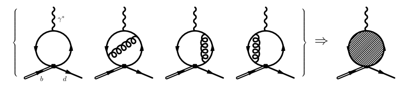
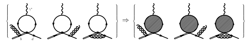
Figure 1: The one- and two-loop factorizable quark loop amplitudes and the all-orders factorizable amplitude that replaces them. Nonfactorizable contributions, where the gluon connects the quark-loop and the heavy-light current or radiates off the quark-loop, are kept perturbative and are not replaced by the KS function.

Secondly the function $h(y_{q})$ appears at leading power in the $\Lambda_{\text{QCD}}/m_{b}$ OPE for $\bar{B}\to X_{d}\ell^{+}\ell^{-}$, and also at leading power in the $\Lambda_{\text{QCD}}/Q$ OPE for $e^{+}e^{-}\to\text{hadrons}$. However, there are power-suppressed effects in $e^{+}e^{-}\to\text{hadrons}$ which appear in $\bar{B}\to X_{d}\ell^{+}\ell^{-}$ at leading power, depicted in figure 2. The light quarks and gluons couple strongly to the QCD vacuum and form $\mathcal{O}(\Lambda_{\text{QCD}})$ condensates: $\braket{\bar{q}q},\braket{GG}$, etc. This is captured by the dispersive analysis which evaluates the factorized hadronic “blob” for both positive and negative $q^{2}$. This neatly encapsulates why the dispersive analysis improves upon a purely perturbative calculation: it resums not only the coupling expansion but also an implicit power expansion in $\Lambda_{\text{QCD}}/Q.$

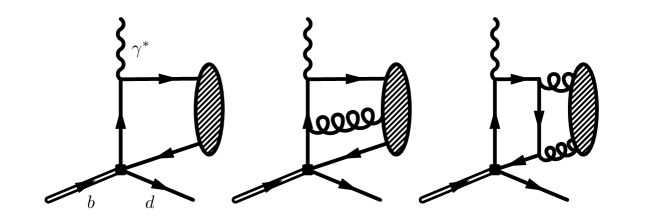
Figure 2: Schematic representation of QCD condensates that appear in $\bar{B}\to X_{d}\ell^{+}\ell^{-}$ at leading power.

4.1.1 Experimental inputs

For the flavour threshold regions we use a compilation of all available data on the hadronic R-ratio Keshavarzi:2018mgv , in which the data is provided in center of mass energy points with a total point-to-point covariance matrix. The BESII data Ablikim:2007gd dominates the statistics in the charm threshold region. The broad oscillation at $\sqrt{s}\sim 1.6\text{ GeV}$ due to the phase space enhancements of isobar processes including $e^{+}e^{-}\to\rho^{+}\rho^{-}\to\pi^{+}\pi^{-}\pi^{0}\pi^{0}$ has been resolved by precise measurements of multi-body final states at BABAR TheBaBar:2017vzo ; Aubert:2005eg ; Aubert:2007ef ; TheBABAR:2017aph ; Aubert:2006jq ; Lees:2014xsh ; Aubert:2007ur ; Aubert:2007ym ; TheBABAR:2018vvb ; TheBABAR:2017vgl . The total nonstrange vector spectral function from $\tau$ decays is taken from ALEPH Davier:2013sfa . A compilation of the data is shown in figure 3. We do not use the strange spectral function because the vector (V) and axial vector (A) contributions are more difficult to distinguish experimentally in this case, and are currently only available in the form V+A.

We supplement this data outside of the resonance region with the results of the program Rhad Harlander:2002ur for computing the hadronic R-ratio up to ${\cal O}(\alpha_{s}^{4})$ in perturbation theory. The only inputs into the program are the $\overline{\text{MS}}$ mass $\overline{m}_{c}(\overline{m}_{c})=1.275(25)$ GeV and $\alpha_{s}(M_{Z})=0.1181(11)$ from table 5, $\overline{m}_{b}(\overline{m}_{b})=4.18(4)\text{ GeV}$ and $\overline{m}_{t}(\overline{m}_{t})=160(5)\text{ GeV}$ Tanabashi:2018oca . The default decoupling scales $\mu_{c}=2m_{c}$, $\mu_{b}=m_{b}$ and $\mu_{t}=m_{t}$ are used, and the scale is varied between $\sqrt{s}/2<\mu<2\sqrt{s}$ to estimate the effect of higher order corrections. In our data-driven approach, we integrate the data directly rather than fit it to a certain model for the resonances.

Figure 3: The hadronic R-ratio Keshavarzi:2018mgv and spectral function from hadronic $\tau$ decay Davier:2013sfa . Under isospin considerations, $3V_{1d}$ is to be compared with the isovector contribution to $R_{\text{had}}$ (from the $\rho$ resonance) with the discrepancy due to the $\omega$ shown in the subfigure. Flavour $SU(3)$ symmetry predicts $R_{\text{had}}=4V_{1d}$. For further details see section 4.1.3.

4.1.2 Charm resonances at high $q^{2}$

Below open charm threshold, to a good approximation, $\text{Im}[h^{\text{KS}}_{c}]$ only has support near the masses of the $\psi$ and $\psi^{\prime}$ resonances, which may eventually decay into light hadrons but resonate through a $c\bar{c}$ current. Above open charm threshold, and below the matching point to perturbation theory with $n_{f}=4$ flavours at $\sqrt{s}=6\text{ GeV}$, the contribution to the R-ratio from the light quarks is perturbative and can be subtracted from the measured spectrum.

$$\text{Im}[h^{\text{KS}}_{c}]=\left\{\begin{array}[]{ll}0\,,&~{}\sqrt{s}<3\text{ GeV},\\[8.0pt] \dfrac{\pi}{3}\left(R_{\text{had}}-R_{uds}^{\text{pert}}\right)\,,&~{}3\text{ GeV}<\sqrt{s}<6\text{ GeV},\\[10.0pt] \dfrac{\pi}{3}R_{c}^{\text{pert}}\,,&~{}\sqrt{s}>6\text{ GeV}\end{array}\right.$$ (60)

We note that a charmonium resonance can form from a vector current of light quarks in $e^{+}e^{-}\to\text{hadrons}$ through single photon or three gluon exchange. This mixing has a substantial effect for the CP asymmetry in $\bar{B}\to X_{d}\psi$ decays Dunietz:1993cg ; Soares:1994vi . Since the QED correction contributes to the present calculation without logarithmic enhancement, we neglect it and the comparable QCD correction and we expect in this case no major nonperturbative enhancement away from the $\psi$ and $\psi^{\prime}$ resonances.

4.1.3 Light quark resonances at low $q^{2}$

The most important new feature for the light quark resonances which we introduce in this paper is to include matrix elements $\langle J_{q}J_{q^{\prime}}\rangle_{q\neq q^{\prime}}$ involving different light-quark currents at very low $q^{2}$. As a consequence, $R_{\rm had}$ alone is not sufficient to extract $\text{Im}[h^{\text{KS}}_{u,d,s}(q^{2})]$.

Figure 4: “Hairpin-turn” diagram in QCD which is ${\cal O}(\alpha_{s}^{3})$-suppressed in perturbation theory, and the origin of its nonperturbative enhancement for low momentum transfer.

The dominant contributions to the $e^{+}e^{-}\to\text{hadrons}$ OPE are from $\langle J_{q}J_{q}\rangle$ for $q=u,d,s$ as they enter at $\mathcal{O}(\alpha_{s}^{0})$. The leading power contributions to $\langle J_{q}J_{q^{\prime}}\rangle_{q\neq q^{\prime}}$ (see left panel of figure 4) are $\mathcal{O}(\alpha_{s}^{3})$ and therefore very small. An expression for these contributions can be found in Harlander:2002ur . This is what lead the authors of ref. Kruger:1996dt to systematically neglect all terms with $q\neq q^{\prime}$ in (51). Unfortunately, at low $q^{2}$ the OPE for $e^{+}e^{-}\to\text{hadrons}$ breaks down and we have to adopt a sum-over-hadrons picture. For instance, at very low $q^{2}$ $(\;\raisebox{-3.00003pt}{$\stackrel{{\scriptstyle\displaystyle<}}{{\sim}}$}\;1\text{ GeV}^{2})$ the dominant hadronic final states are two and three pions – corresponding essentially to the $\rho$ and $\omega$ resonances – and $\langle J_{u}J_{d}\rangle\sim\langle J_{u}|\pi\pi(\pi)\rangle\langle\pi\pi(\pi)|J_{d}\rangle\sim\langle J_{u}|\pi\pi(\pi)\rangle\langle\pi\pi(\pi)|J_{u}\rangle\sim\langle J_{u}J_{u}\rangle$. At larger $q^{2}$ $(\;\raisebox{-3.00003pt}{$\stackrel{{\scriptstyle\displaystyle>}}{{\sim}}$}\;4\text{ GeV}^{2})$ there is a proliferation of multiparticle intermediate states and the OPE result that $\braket{J_{u}J_{d}}\sim 0$ is recovered via dramatic cancellations between various exclusive final states Lipkin:1984sw ; Lipkin:1986av as confirmed by lattice-QCD calculations Isgur:2000ts .

To quantify these effects, it is convenient to work in terms of a basis of neutral isospin currents

$$J_{0}=\frac{J_{u}+J_{d}}{\sqrt{2}},\hskip 14.22636ptJ_{1}=\frac{J_{u}-J_{d}}{\sqrt{2}},\hskip 14.22636ptJ_{s},$$ (61)

where $J_{0},J_{s}$ are singlets under isospin and $J_{1}$ transforms as a vector. The correlation functions of these currents describe the propagation of the relevant degrees of freedom in the low energy resonance region:

$$(q^{2}g^{\mu\nu}-q^{\mu}q^{\nu})\Pi_{ab}(q^{2})=i\int d^{4}x~{}e^{iqx}\braket{0}{T{J_{a}}^{\mu}(0){J_{b}}^{\nu}(x)}{0}.$$ (62)

Note that if the six correlators $\Pi_{ab}$ were known exactly, the six correlators between quark currents $\braket{J_{q_{1}}J_{q_{2}}}$ and finally the KS functions (51) would be determined exactly through simple relations at the operator level. We note in particular that the electromagnetic current and the $u-$quark current are given exactly by

$$J_{u}=\frac{J_{1}+J_{0}}{\sqrt{2}},\hskip 14.22636ptJ_{\text{em}}=\frac{3J_{1}+J_{0}-\sqrt{2}J_{s}}{3\sqrt{2}}.$$ (63)

In the isospin limit, the correlators $\Pi_{10}$ and $\Pi_{1s}$ vanish, (53) and (55) simplify to

$$\Pi_{\gamma}=\frac{9\Pi_{11}+\Pi_{00}+2\Pi_{ss}-2\sqrt{2}\Pi_{0s}}{18},\hskip 14.22636pt\Pi_{\bar{u}d}=\Pi_{11},$$ (64)

and the KS functions simplify to

$$h^{\text{KS}}_{u} =\frac{4\pi^{2}}{9}(3\Pi_{11}+\Pi_{00}-\sqrt{2}\Pi_{0s}),$$

$$h^{\text{KS}}_{d} =\frac{4\pi^{2}}{9}(6\Pi_{11}-2\Pi_{00}+2\sqrt{2}\Pi_{0s}),$$

$$h^{\text{KS}}_{s} =\frac{4\pi^{2}}{9}(4\Pi_{ss}-2\sqrt{2}\Pi_{0s}).$$ (65)

Since the KS functions in the isospin limit depend on the four correlators $\Pi_{11},\Pi_{00},\Pi_{ss},\Pi_{0s}$ and only two observables $R_{\text{had}}$ and $V_{1d}$ are available, additional assumptions are required whose range of applicability depends on the energy.

$$\Big{(}$$ (GeV)

0

Table 3: Imaginary parts of the KS functions in various regions as determined from experimental data. One has $\hat{R}_{\text{had}}=4\pi/9R_{\text{had}}$ and $\hat{V}_{1d}=4\pi/9V_{1d}$.

Below $K\bar{K}$ threshold, in addition to isospin symmetry, we assume that the hidden strange contributions to the final states $\pi^{+}\pi^{-}$ and $\pi^{+}\pi^{-}\pi^{0}$ are small ($\text{Im}[\Pi_{ss}]=\text{Im}[\Pi_{0s}]=0$). Then the Krüger-Sehgal functions as well as $R_{\text{had}}$ and $V_{1d}$ depend only on $\Pi_{00}$ and $\Pi_{11}$, and inverting these equations yields the second column of table 3.

The $\phi$ resonance, which we identify as the region between $K\bar{K}$ and $K\bar{K}\pi$ thresholds, decays predominantly into $\pi^{+}\pi^{-}\pi^{0}$ and $K\bar{K}$ final states, and these contributions are understood as contributions to $\Pi_{ss}$ up to rescattering effects suppressed in $\Pi_{0s}$ and further suppressed in $\Pi_{00}$, which we both neglect. The isovector background dominated by the tail of the $\rho$ is understood from the $\tau$ data, using the isospin correspondence $R^{I=1}_{\text{had}}\to 3V_{1d}$ (see figure 3). This yields the third column of table 3.

Above $K\bar{K}\pi$ threshold, all four correlators $\Pi_{ab}$ appearing in (65) are important. To proceed, we consider the consequences of enlarging the symmetry group to flavour $SU(3)$, introducing the currents:

$$J_{0}^{(3)}=\frac{J_{u}+J_{d}+J_{s}}{\sqrt{3}},\hskip 8.5359ptJ_{3}^{(3)}=\frac{J_{u}-J_{d}}{\sqrt{2}},\hskip 8.5359ptJ_{8}^{(3)}=\frac{J_{u}+J_{d}-2J_{s}}{\sqrt{6}}.$$ (66)

where $J_{0}^{(3)}$ is an $SU(3)$ singlet and $J_{3,8}^{(3)}$ transform as vectors (the subscripts refer to Gell-Mann matrix indices). In the flavour symmetry limit, the correlators $\Pi_{03}^{(3)}$ and $\Pi_{08}^{(3)}$ vanish, $\Pi_{38}^{(3)}$ vanishes by isospin symmetry, and $\Pi_{33}^{(3)}=\Pi_{88}^{(3)}$. Only two independent correlators remain: $\Pi_{33}^{(3)}$ and $\Pi_{00}^{(3)}$. The vacuum polarization and spectral function, however, are independent of $\Pi_{00}^{(3)}$. Therefore flavour symmetry predicts $R_{\text{had}}=4V_{1d}$, to be compared with experiment (figure 3). The difference between $R_{\text{had}}$ and $4V_{1d}$ corresponds to the breaking of flavour symmetry, which is apparent but moderate. In the flavour symmetry limit the Krüger-Sehgal functions are independent of flavour, but there is a systematic error associated to the difference between $R_{\text{had}}$ and $4V_{1d}$. We account for this by introducing standard normal variables $\delta_{u,d,s}$ which are varied in the error analysis (see fourth column of table 3). For $\sqrt{s}>1.65\text{ GeV}$, where there is no reliable $\tau$ data, we assume flavour symmetry, see last column of table 3. The perturbative result from Rhad Harlander:2002ur is used for $\sqrt{s}>3\text{ GeV}$.

By means of this procedure, we obtain the KS functions which are displayed in figure 5 together with the perturbative functions up to two loops. Uncertainties are propagated by generating samples of the data, and for each sample calculating $\text{Im}[h_{q}^{\text{KS}}]$ using table 3 and eq. (60), and subsequently calculating the real part via the integral (59). Note that in this way, estimates of $SU(3)$ breaking and uncertainties in charmonium resonance parameters are included in the error analysis. We investigated the dependence on the subtraction point $s_{0}$ and found it to be small.

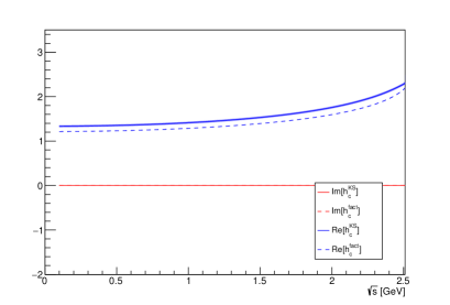
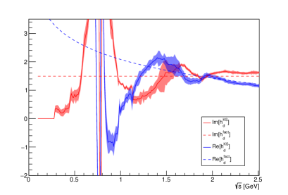
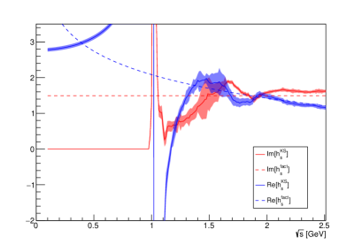
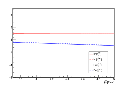
Figure 5: KS functions and the corresponding perturbative functions to two loops in the low- and high-$q^{2}$ region. See text for further details.

4.2 Resolved contributions at low $q^{2}$

As discussed at the beginning of this section, the local heavy mass expansion breaks down if one includes operators beyond the leading ones in the effective field theory. One then finds nonlocal power corrections in the low-$q^{2}$ region which can be systematically analysed within soft-collinear effective theory (SCET). The resolved photon contributions to the inclusive decay $\bar{B}\rightarrow X_{s(d)}\ell^{+}\ell^{-}$ contain subprocesses in which the virtual photon couples to light partons instead of connecting directly to the effective weak-interaction vertex. These resolved contributions of the $\bar{B}\rightarrow X_{s}\ell^{+}\ell^{-}$ decay were calculated in SCET in the presence of an $M_{X}$ cut to order $1/m_{b}$ Hurth:2017xzf ; Benzke:2017woq . They can be represented as the convolution integrals of a jet-function, characterizing the hadronic final state $X_{s(d)}$, and of a soft (shape) function which is defined by a non-local heavy-quark effective theory matrix element. The hard contribution is factorized into the Wilson coefficients. It was explicitly shown Hurth:2017xzf ; Benzke:2017woq , that the resolved contributions stay nonlocal when the hadronic cut is released and thus, represent an irreducible uncertainty. The support properties of the shape function imply that the resolved contributions (besides the ${\cal O}_{8g}-{\cal O}_{8g}$ one) are almost cut-independent.

Within the inclusive decay $\bar{B}\to X_{d}\ell^{+}\ell^{-}$, there are four resolved contributions at leading order in $1/m_{b}$ for the decay rate, namely from the interference terms ${\cal O}_{7\gamma}-{\cal O}_{8g}$,  ${\cal O}_{8g}-{\cal O}_{8g}$, and ${\cal O}^{c}_{1}-{\cal O}_{7\gamma}$, but also ${\cal O}^{u}_{1}-{\cal O}_{7\gamma}$ . For the $b\to d$ case the resolved contributions need some obvious modifications compared to the $b\to s$ case which was calculated in Refs. Hurth:2017xzf ; Benzke:2017woq : The CKM parameter combinations $\lambda_{i}^{s}=V_{is}^{\ast}V_{ib}$ have to be replaced by $\lambda_{i}^{d}=V_{id}^{\ast}V_{ib}$ and $s$-quark fields have to be replaced by $d$-quark fields in the shape functions. These modifications only change the numerical results.

It is well-known that the ${\cal O}^{u}_{1}-{\cal O}_{7\gamma}$ contribution is CKM-suppressed in the $b\to s$ case, but not in the $b\to d$ case. However, both in $b\to d$ and in $b\to s$, this contribution from the $u$-quark loop vanishes within the CP averaged quantities at the order $1/m_{b}$ as one can derive from the results given in Ref. Benzke:2017woq : If we start with the ${\cal O}^{c}_{1}-{\cal O}_{7\gamma}$ contribution in eq. (6.3) of ref. Benzke:2017woq and consider the penguin functions given in eqs. (4.4) and (4.5) of that reference, which enter the jet function, we find in the limit $m_{c}\to m_{u}=0$ that the $\omega_{1}$ integral reduces to

$$\int d\omega_{1}\frac{1}{\omega_{1}+i\epsilon}\times\frac{1}{\omega_{1}}\left[\,\,\omega_{1}\,\,\right]\,g_{17}(\omega,\omega_{1},\mu)\,.$$ (67)

The trace formalism of HQET (see ref. Benzke:2010js ) implies that

$$\int_{-\infty}^{\bar{\Lambda}}\!d\omega\,g_{17}(\omega,\omega_{1},\mu)=\int_{-\infty}^{\bar{\Lambda}}\!d\omega\,(g_{17}(\omega,-\omega_{1},\mu))^{*}.$$ (68)

Moreover, it is a consequence of PT invariance that $g_{17}$ is real. Thus, the integration of $\omega_{1}$ leads to the result that the interference term ${\cal O}^{u}_{1}-{\cal O}_{7\gamma}$ vanishes within the integrated CP averaged rate. This is a crucial result for all CP-averaged inclusive $b\to d\ell^{+}\ell^{-}$ quantities because previously no estimate for this up-quark loop of order $\Lambda_{\rm QCD}/m_{b}$ was available (see ref. Buchalla:1997ky ) and thus represented the main uncertainty in the inclusive $b\to d\ell^{+}\ell^{-}$ observables. Further insight into the moments of $g_{17}$ was recently given in Gunawardana:2019gep .

The calculation of the other (nontrivial) resolved contributions given in refs. Hurth:2017xzf ; Benzke:2017woq starts with the explicit form of the shape functions as HQET matrix elements and derives general properties of those. One can then use various model functions which have all these properties to get conservative estimates of the resolved contributions by maximizing the value of the convolution integral of the subleading shape function with the perturbatively calculable jet function (for more details see ref. Benzke:2017woq ). We are interested in the relative magnitude of the resolved contributions compared to the total decay rate. We finally get for the various contributions at order $1/m_{b}$ in the $b\to s$ and $b\to d$ decays:

$${\mathcal{F}}^{s}_{17}\in[-0.5,+3.4]\,\%, {\mathcal{F}}^{d}_{17}\in[-0.6,+4.1]\,\%,{\mathcal{F}}^{d,s}_{78}\in[-0.2,-0.1]\,\%, {\mathcal{F}}^{d,s}_{88}\in[0,0.5]\,\%\,.$$

Summing them up in a conservative way we arrive at

$${\mathcal{F}}^{d}_{{1/m_{b}}}\in[-0.8,+4.5]\,\%,\,\,{\mathcal{F}}^{s}_{{1/m_{b}}}\in[-0.7,+3.8]\,\%.$$ (70)

It was found Hurth:2017xzf ; Benzke:2017woq that at leading order in $1/m_{b}$ there is no resolved contribution to the forward-backward asymmetry. This starts at order $1/m_{b}^{2}$ only with an interference term of ${\cal O}^{c}_{1}-{\cal O}_{10}$ for example. Also the resolved ${\cal O}^{c}_{1}-{\cal O}_{9}$ term, contributing to the rate, only occurs at the subleading $1/m_{b}^{2}$ order. This is a consequence of the fact that the virtual photon is hard-collinear and not hard in the low-$q^{2}$ region as explicitly shown in refs. Hurth:2017xzf ; Benzke:2017woq . On the other hand, these $1/m_{b}^{2}$ terms might be numerically relevant due to the large ratio $|C_{9/10}|\sim 13|C_{7\gamma}|$ of Wilson coefficients which necessitates their calculation Benzkeworkinprogress .

Because of the opposite sign of $C_{9}$ compared to $C_{7}$ one can also expect the same behaviour of the resolved ${\cal O}^{c}_{1}-{\cal O}_{9}$ term with respect to ${\cal O}^{c}_{1}-{\cal O}_{7\gamma}$. We therefore estimate the interval of the missing ${\cal O}^{c}_{1}-{\cal O}_{9}$ piece to be reversed with respect to eq. (LABEL:eq:Fijresolved) and add it linearly to the interval of the corresponding ${\cal O}^{c}_{1}-{\cal O}_{7\gamma}$ term,

$${\mathcal{F}}^{s}_{1(7+9)}\in[-3.9,+3.9]\,\%, {\mathcal{F}}^{d}_{1(7+9)}\in[-4.7,+4.7]\,\%.$$ (71)

In our final calculation we combine this result with the ${\cal O}_{7\gamma}-{\cal O}_{8g}$ and ${\cal O}_{8g}-{\cal O}_{8g}$ interferences from (LABEL:eq:Fijresolved) to obtain

$${\mathcal{F}}^{s}\in[-4.1,+4.3]\,\%, {\mathcal{F}}^{d}\in[-4.9,+5.1]\,\%.$$ (72)

For the first nontrivial resolved contribution to the forward backward asymmetry from the ${\cal O}^{c}_{1}-{\cal O}_{10}$ term at order $1/m_{b}^{2}$ we add an error of $\pm 5\%$ in our final result before an explicit estimate is available Benzkeworkinprogress .

4.3 Nonfactorizable power contributions at high $q^{2}$

Power corrections due to operators beyond the leading ones also exist in the high-$q^{2}$ region. The only available pieces are the nonfactorizable charm- and up-loop diagrams of the four-quark operator ${P}_{1,2}$ with a soft gluon which interacts with the spectator cloud. However, in the high-$q^{2}$ region the dilepton mass $q^{2}$ is a hard momentum and any cut on the hadronic mass has no influence in the high-$q^{2}$ region. Thus, the kinematic situation is a different one compared to the low-$q^{2}$ region, in particular there is no nonlocal shape function involved. In this case the original treatment of Voloshin Voloshin:1996gw is applicable which leads to a local expansion again Buchalla:1997ky .

Here we briefly recall the crucial issues of the calculational details presented in ref. Buchalla:1997ky . The nonperturbative effect due to the $\bar{s}b\gamma g$ vertex is represented by a form factor $\overline{F}$ which depends on the two variables $r=q^{2}/(4m_{c}^{2})$ and $t=k\cdot q/(2m_{c}^{2})$ where $k$ denotes the soft gluon momentum ($k^{2}=0$) and $q$ the virtual photon momentum. The form factor ${\overline{F}}(r+t,t)$ is given in eq. (4.28) of ref. Buchalla:1997ky . One may expand ${\overline{F}}$ in powers of $t$ . In the high-$q^{2}$ region $q$ is a hard momentum (of order $m_{b}$) and $k$ is a soft momentum. Thus, if $m_{b}\Lambda_{QCD}/(2m_{c}^{2})$ is small the first term in the expansion about $t=0$ can be regarded as dominating. Moreover, one may additionally expand the form factor also in $1/r$ which is of order $4m_{c}^{2}/m_{b}^{2}$. The authors of ref. Buchalla:1997ky then keep only the leading term in $1/r$ in each of the coefficients of $t^{n}$ and find

$${\overline{F}}(r+t,t)\approx\sum^{\infty}_{n=0}(-1)^{n+1}\frac{3}{(n+2)r^{n+1}}t^{n}=-\frac{3}{2r}+\frac{t}{r^{2}}+\ldots$$ (73)

This means that the leading corrections to the $t=0$ result are suppressed by $t/r=2k\cdot q/q^{2}$. An additional numerical test Buchalla:1997ky suggests that the $t=0$ term is the dominating one in the high-$q^{2}$ region. The concrete results for the leading $1/m_{c}^{2}$ term are given in section 3.3. If we consider the corresponding nonfactorizable contribution with an up-quark loop in the high-$q^{2}$ region, one finds that the leading term is of order $\Lambda^{2}_{\text{QCD}}/q^{2}$ and corrections are suppressed by powers of $t/r\sim\Lambda_{\text{QCD}}/(2\sqrt{q^{2}})$ Buchalla:1997ky . The leading order results for the up-quark are also given in section 3.3.

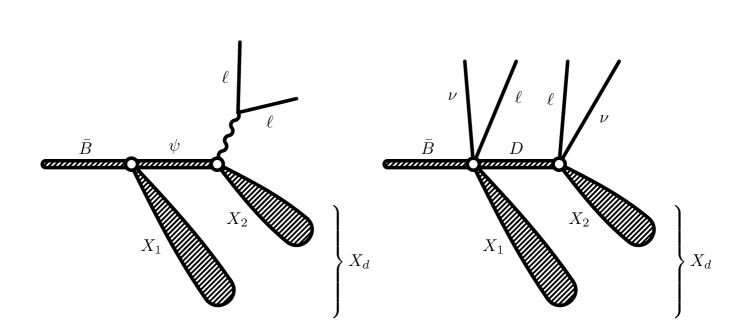
Figure 6: Long distance backgrounds not removed by $q^{2}$ cuts. Left: Charmonium cascade lowering $q^{2}$ to the perturbative window. Right: Double semileptonic background through sequential weak decays.

4.4 Charmonium cascade backgrounds

Another long distance effect at low $q^{2}$ are the cascade decays $\bar{B}\to X_{1}(c\bar{c}\to X_{2}\ell^{+}\ell^{-})$ through the radiative decay of a narrow charmonium resonance $\eta_{c},\eta_{c}^{\prime},\psi,\psi^{\prime},\chi_{cJ},h_{c}$ or exotic XYZ state, collectively referred to as $c\bar{c}$, as depicted in the left panel of figure 6. In contrast to the infamous $\psi\to\ell^{+}\ell^{-}$, for example the decay $\psi\to\eta^{\prime}\ell^{+}\ell^{-}$ completely escapes the upper cut $q^{2}=\text{6 GeV}^{2}$ in $\bar{B}\to X_{q}\ell^{+}\ell^{-}$:

$$4m_{\ell}^{2}<q^{2}<(M_{c\bar{c}}-M_{X_{2}})^{2}.$$ (74)

In the following we focus on $\bar{B}\to X_{s}(c\bar{c}\to X_{2}\ell^{+}\ell^{-})$ with the understanding that the relative effect of the cascades on $\bar{B}\to X_{d}\ell^{+}\ell^{-}$ and $\bar{B}\to X_{s}\ell^{+}\ell^{-}$ are roughly the same due to the CKM scaling of charmonium production:

$$\frac{\Gamma(B\to X_{s}c\bar{c})}{\Gamma(B\to X_{d}c\bar{c})}\sim\frac{\Gamma(B\to X_{s}\ell^{+}\ell^{-})}{\Gamma(B\to X_{d}\ell^{+}\ell^{-})}\sim\left|\frac{V_{cb}V_{cs}}{V_{cb}V_{cd}}\right|^{2}.$$ (75)

Charmonium production from $B$-decays is reasonably well described by an expansion in the heavy quark velocity (NRQCD) Beneke:1998ks ; Beneke:1999gq and has been investigated by several experiments, summarized in table 4. The inclusive spectra from $c\bar{c}\to X\ell^{+}\ell^{-}$ are not yet available, although the decays $\psi\to(\pi^{0},\eta,\eta^{\prime})\ell^{+}\ell^{-}$ have been measured at BESIII Ablikim:2014nro ; Ablikim:2018eoy ; Ablikim:2018bhf , and happen to be the most important. We note that the dilepton decays between charmonium states Ablikim:2017kia ; Ablikim:2019jqp ; Aaij:2017vck are not pertinent to $\bar{B}\to X_{s}\ell^{+}\ell^{-}$ because the leptons in this case come with invariant mass below the difference in charmonium masses, which is less than $1\text{ GeV}$.

Radiative and dilepton charmonium decays have been mentioned in the context of $\bar{B}\to X_{s}\gamma$ Misiak:2000jh ; Buchalla:1997ky ; Beneke:2009az and $\bar{B}\to X_{s}\ell^{+}\ell^{-}$ Buchalla:1997ky . The background in $\bar{B}\to X_{s}\ell^{+}\ell^{-}$ could simply be subtracted by vetoing events where the two leptons and any permutation of light hadrons reconstruct any of the charmonium masses. However, only the direct leptonic decay of $\psi$ and $\psi^{\prime}$ were interpreted as background to $\bar{B}\to X_{s}\ell^{+}\ell^{-}$ at Belle Sato:2014pjr ; Iwasaki:2005sy and BaBar Lees:2013nxa . This is problematic because there are also cascade decays of the type $\bar{B}\to X_{1}\psi\to X_{1}X_{2}\ell^{+}\ell^{-}$ that form a reducible background in the limit in which interference between the cascade and the genuine short distance $\bar{B}\to X_{s}\ell^{+}\ell^{-}$ amplitudes is negligible. On general grounds this interference is expected to be much smaller than the square of the cascade amplitude. If estimates of the cascade contributions are low enough, we can argue that interference effects can be neglected, implying that these cascades are a reducible background that can be either separately calculated and subtracted or experimentally removed. As we show below, cascades in $\bar{B}\to X_{s}\ell^{+}\ell^{-}$ satisfy this requirement, but only after taking into account the cut on the invariant mass of the $X_{s}$ system which is required experimentally to remove the double semileptonic background, as shown in the right panel of figure 6. In the rest of this subsection we show how to estimate the impact of the $M_{X}$ cuts on a generic cascade.

	$\mathcal{B}\times 10^{3}$		$\mathcal{B}\times 10^{5}$
$\bar{B}\to X_{s}\psi$	$7.8\pm 0.4$	$\psi\to\eta\ell^{+}\ell^{-}$	$1.43\pm 0.07$
$\bar{B}\to X_{s}\psi^{\prime}$	$3.07\pm 0.21$	$\psi\to\eta^{\prime}\ell^{+}\ell^{-}$	$6.59\pm 0.18$
$\bar{B}\to X_{s}\chi_{c1}$	$3.09\pm 0.22$	$\psi\to\pi^{0}\ell^{+}\ell^{-}$	$0.076\pm 0.014$
$\bar{B}\to X_{s}\chi_{c2}$	$0.75\pm 0.11$	$\psi^{\prime}\to\eta^{\prime}\ell^{+}\ell^{-}$	$0.196\pm 0.026$
$\bar{B}\to X_{s}\eta_{c}$	$4.88\pm 0.97$ Aaij:2014bga
$\bar{B}\to X_{s}\chi_{c0}$	$3.0\pm 1.0$ Aaij:2017tzn
$\bar{B}\to X_{s}h_{c}$	$2.4\pm 1.0^{\dagger}$ Beneke:1998ks
$\bar{B}\to X_{s}\eta_{c}^{\prime}$	$0.12\pm 0.22^{\dagger}$ Fan:2011aa

Table 4: Branching ratios of (direct) inclusive $B$-decay into charmonium, and of vector charmonium dilepton decay to light pseudoscalars. Numbers marked with $\dagger$ are NRQCD estimates, and unless otherwise stated are taken from the PDG Tanabashi:2018oca .

The relative momentum between $X_{1}$ and $X_{2}$ implies that the cascade events come with somewhat large total $M_{X}$ when the two systems are combined. Since it is already necessary to measure $\bar{B}\to X_{s}\ell^{+}\ell^{-}$ with an $M_{X}$ cut to remove the double semileptonic background, if cascade events were efficiently removed by this cut, then there would be no need for their further consideration. The invariant mass of the $X$ system is given by

$$M_{X}^{2} =M_{X_{1}}^{2}+M_{X_{2}}^{2}+2E_{X_{1}}E_{X_{2}}\left(1-\frac{|\vec{p}_{X_{1}}||\vec{p}_{X_{2}}|}{E_{X_{1}}E_{X_{2}}}\cos\theta_{X}\right),$$ (76)

$$E_{X_{1}} =\frac{M_{B}^{2}-M_{c\bar{c}}^{2}-M_{X_{1}}^{2}}{2M_{c\bar{c}}},$$ (77)

$$E_{X_{2}} =\frac{M_{c\bar{c}}^{2}+M_{X_{2}}^{2}-q^{2}}{2M_{c\bar{c}}},$$ (78)

where $\theta_{X}$ is the angle between the $X_{1}$ and $X_{2}$ systems in the charmonium rest frame. It is interesting to consider the minimum value of $M_{X_{2}}$ such that $M_{X}>M_{X}^{\text{cut}}$ for all $q^{2}$ and $M_{X_{1}}$. This is given in closed form by

$$M_{X_{2}}^{\text{cut}}=\frac{M_{c\bar{c}}M_{X}^{\text{cut}}}{M_{B}}$$ (79)

and corresponds to the extreme values $\theta_{X}=0$, $M_{X_{1}}=0$ and $q^{2}=0$. States with $M_{X_{2}}$ heavier than (79) are completely removed by the $M_{X}$ cut. In the case of $\psi$-decays with $M_{X}^{\text{cut}}=2\text{ GeV}$, $M_{X_{2}}^{\text{cut}}\sim 1.2\text{ GeV}$ (the minimum mass $M_{X_{1}}=M_{K}$ and cut at $q^{2}=1\text{ GeV}^{2}$ causes this to be slightly smaller). The decays $\psi\to(\pi,\eta,\eta^{\prime})\ell^{+}\ell^{-}$ and nonresonant S- or D-wave $\psi\to 2\pi\ell^{+}\ell^{-}$ are therefore of interest, while the resonances $\psi\to(f_{0},f_{2})\ell^{+}\ell^{-}$ are cut away. Inferring from the photon energy spectrum in $\psi\to 2\pi\gamma$, nonresonant $\psi\to 2\pi\ell^{+}\ell^{-}$ is probably very small. Similarly $h_{c}\to(\eta,\eta^{\prime},2\pi)\ell^{+}\ell^{-}$ and $\chi_{c1}\to(\rho,\omega)\ell^{+}\ell^{-}$ are of interest but they are suppressed by an order of magnitude compared with the $\psi$ decays in the real photon case:

$$\frac{\mathcal{B}(B\to X\chi_{c1})\mathcal{B}(\chi_{c1}\to\rho\gamma)}{\mathcal{B}(B\to X\psi)\mathcal{B}(\psi\to\eta\gamma)}\sim 0.08\,,\hskip 28.45274pt\frac{\mathcal{B}(B\to Xh_{c})\mathcal{B}(h_{c}\to\eta\gamma)}{\mathcal{B}(B\to X\psi)\mathcal{B}(\psi\to\eta\gamma)}\sim 0.14\ .$$ (80)

The sequence $\bar{B}\to X_{1}\psi^{\prime}$, $\psi^{\prime}\to 2\pi\psi$, $\psi\to\eta(\eta^{\prime})\ell^{+}\ell^{-}$ is also of interest but the total $M_{X}$ from $X_{1}$, $2\pi$ and $\eta(\eta^{\prime})$ is largish. Finally, we observe that the branching ratio of $\psi\to\pi\ell^{+}\ell^{-}$ is about two orders of magnitude smaller compared to $\psi\to\eta(\eta^{\prime})\ell^{+}\ell^{-}$ (see table 4). Hence the conclusion is that the direct decay $\psi\to\eta\ell^{+}\ell^{-}$ and $\psi\to\eta^{\prime}\ell^{+}\ell^{-}$ dominate the background to $\bar{B}\to X_{s}\ell^{+}\ell^{-}$ from all charmonium radiative decays in the presence of a cut $M_{X}<2\text{ GeV}$.

The helicity-projected rates for $\psi\to\eta(\eta^{\prime})\ell^{+}\ell^{-}$ normalized to the rate $\psi\to\eta(\eta^{\prime})\gamma$ can be calculated from first principles in terms of a single $q^{2}$-dependent form factor Landsberg:1986fd . The angular distribution is simply given in terms of the polarization $\alpha$ as

$$\frac{d\Gamma(\psi\to\eta\ell^{+}\ell^{-})}{d\cos\theta_{X}} \propto 1+\alpha\cos^{2}\theta_{X}\;.$$ (81)

Due to the V$-$A coupling of the underlying transition $b\to sc\bar{c}$, $\bar{B}\to\psi X_{1}$ prefers the longitudinal polarization Anderson:2002md ; Aubert:2002hc with corrections quantified in NRQCD Fleming:1996pt ; this fact reduces the background from the cascades because $\eta(\eta^{\prime})$ and $X_{1}$ cannot be collinear through the dominant longitudinal polarization. The resulting distribution in the $[q^{2},M_{X}]$ plane for the decays into $\eta$ and $\eta^{\prime}$ are presented in figure 7, where we take for simplicity a constant value $\alpha=-0.59$ corresponding to the low $M_{X_{1}}$ bin of the BaBar measurement: this causes the $M_{X}$ cut to be more efficient by about 20%.

The contributions of the cascade into $\eta$ and $\eta^{\prime}$ to the total $\bar{B}\to X_{s}\ell^{+}\ell^{-}$ branching ratio before any $M_{X}$ cut are $1\%$ and $5\%$, respectively. After imposing $M_{X}<2\;{\rm GeV}$ these effects are diluted to $0.05\%$ and $0.0005\%$. Keeping in mind that the impact of the $M_{X}$ cut on the non-resonant decay is about $60\%$, we conclude that the experimental cut on $M_{X}$ completely removes any pollution from cascade charmonium decays. This conclusion persists as long as the $M_{X}$ cut is at most $3\;{\rm GeV}$.

Figure 7: The background from $B^{+}\to K^{+}(\psi\to h\ell^{+}\ell^{-})$ with $h=\pi,\eta,\eta^{\prime}$ on the ${\bar{B}\to X_{s}\ell^{+}\ell^{-}}$ phase space. The color bar corresponds to the branching ratio differential in dilepton mass ($\sqrt{s}$) and hadronic mass ($M_{X}$), in units of $10^{-8}~{}\text{GeV}^{-2}$. The outlined box indicates the $1~{}\text{GeV}^{2}<q^{2}<6~{}\text{GeV}^{2}$ and $M_{K}<M_{X}<2~{}\text{GeV}$ cuts. A single-pole parameterization of the transition form factor Landsberg:1986fd with the same $\Lambda=3.686\text{ GeV}$ for $\pi,\eta,\eta^{\prime}$ was used to generate the plots. The fact that the cuts are less efficient for $\psi\to\pi$ is not problematic due to the small rate of this channel.

5 Inputs

The numerical inputs used in the phenomenological analysis are presented in table 5. Most of the quantities listed in the table have been determined with great accuracy and will not be discussed further. The required HQET matrix elements, on the other hand, necessitate a more in depth discussion.

$$\alpha_{s}(M_{z})=0.1181(11)$$

 Charles:2004jd

 Charles:2004jd  Amhis:2012bh ; Schwanda:2013bg

 Charles:2004jd  Charles:2004jd

 Charles:2004jd  Charles:2004jd

 Amhis:2016xyh

 Alberti:2014yda

Gambino:2016jkc

 Gambino:2016jkc

 Gambino:2016jkc

Table 5: Numerical inputs used in the phenomenological analysis. Unless specified otherwise, they are taken from PDG Tanabashi:2018oca . In order to avoid somewhat uncontrolled non-perturbative effects, we use the pole mass of the top quark obtained from cross section measurements. The CKM matrix elements have been obtained by propagating the uncertainties on the four CKM Wolfenstein parameters ($\lambda$, $A$, $\bar{\rho}$ and $\bar{\eta}$) taken from the global fit as of Summer 2018 presented by the CKMfitter Group Charles:2004jd . All HQET matrix elements are calculated between physical $B$ mesons. Only the combination $\lambda_{2}^{\rm eff}\equiv\lambda_{2}-\rho_{2}/m_{b}$ enters in $\bar{B}\to X_{d,s}\ell^{+}\ell^{-}$. The annihilation matrix elements required for $\bar{B}\to X_{d}\ell^{+}\ell^{-}$ and $\bar{B}\to X_{s}\ell^{+}\ell^{-}$ are $(f_{u},f_{d})$ and $(f_{u}^{0},f_{u}^{\pm},f_{s})$, respectively, where we use the notation $f_{q}\equiv(f_{q}^{0}+f_{q}^{\pm})/2$. As explained in the text we express them in terms of the valence and non-valence matrix elements, $f_{\text{V}}$ and $f_{\text{NV}}$, and the flavour $SU(3)$ and the isospin breaking differences $[\delta f]_{SU(3)}$ and $[\delta f]_{SU(2)}$.

For our phenomenological study, we need the matrix elements of the following dimension five and six operators:

$$\lambda_{1} \equiv\frac{1}{2m_{B}}\langle B|\bar{h}_{v}(iD)^{2}h_{v}|B\rangle\;,$$ (82)

$$\lambda_{2} \equiv\frac{1}{12m_{B}}\langle B|\bar{h}_{v}(-i\sigma_{\mu\nu})G^{\mu\nu}h_{v}|B\rangle\;,$$ (83)

$$\rho_{1} \equiv\frac{1}{2m_{B}}\langle B|\bar{h}_{v}iD_{\mu}(iv\cdot D)iD^{\mu}h_{v}|B\rangle\;,$$ (84)

$$\rho_{2} \equiv\frac{1}{6m_{B}}\langle B|\bar{h}_{v}iD^{\mu}(iv\cdot D)iD^{\nu}h_{v}(-i\sigma_{\mu\nu})|B\rangle\;,$$ (85)

$$f^{a}_{q} \equiv\frac{1}{2m_{B}}\langle B^{a}|Q_{1}^{q}-Q_{2}^{q}|B^{a}\rangle\;,$$ (86)

where $a=0,\pm$ denotes the charge of the meson, $q=u,d,s$ is the flavour of the spectator quark and Voloshin:2001xi

$$Q_{1}^{q} =\bar{h}_{v}\gamma_{\mu}(1-\gamma_{5})q\;\bar{q}\gamma^{\mu}(1-\gamma_{5})h_{v}\;,$$ (87)

$$Q_{2}^{q} =\bar{h}_{v}(1-\gamma_{5})q\;\bar{q}(1+\gamma_{5})h_{v}\;.$$ (88)

The leading matrix elements $\lambda_{1,2}$ and $(\rho_{1,2},f_{q}^{a})$ scale as $m_{b}^{-2}$ and $m_{b}^{-3}$ respectively. The matrix elements $\lambda_{2}$ and $\rho_{2}$ appear only in the combination

$$\lambda_{2}^{\rm eff} \equiv\lambda_{2}-\frac{\rho_{2}}{m_{b}}\;.$$ (89)

Note that we consider exclusively HQET matrix elements between physical $B$ mesons. Matrix elements in the infinite mass limit are independent of the heavy quark mass and are sometimes used when combining fits involving both $b$- and $c$-hadrons. For the two leading dimension five operators the relation between these matrix elements is:

$$\lambda_{1} \equiv\frac{1}{2m_{B}}\langle B|\bar{h}_{v}(iD)^{2}h_{v}|B\rangle=\frac{1}{2m_{B}}\langle H_{\infty}|\bar{h}_{v}(iD)^{2}h_{v}|H_{\infty}\rangle+\frac{\tau_{1}+3\tau_{2}}{m_{b}}\;,$$ (90)

$$\lambda_{2} \equiv\frac{1}{12m_{B}}\langle B|\bar{h}_{v}(-i\sigma_{\mu\nu})G^{\mu\nu}h_{v}|B\rangle=\frac{1}{12m_{B}}\langle H_{\infty}|\bar{h}_{v}(-i\sigma_{\mu\nu})G^{\mu\nu}h_{v}|H_{\infty}\rangle+\frac{\tau_{3}+3\tau_{4}}{m_{b}}\;,$$ (91)

where the non-local matrix elements $\tau_{i}$ can be found, for instance, in ref. Gremm:1996df .

The $\lambda_{i}$ and $\rho_{i}$ matrix elements can be extracted from measurements of several leptonic and hadronic moments of the inclusive $\bar{B}\to X_{c}\ell\nu$ spectrum, under the assumption that its shape is unaffected by new physics effects. The most recent analysis has been presented in ref. Gambino:2016jkc , where the results are expressed in the kinetic scheme Bigi:1994ga ; Bigi:1997fj ; Bigi:1996si ; Gambino:2004qm . In this scheme the renormalized matrix elements at a scale $\mu=1$ GeV are connected to the usual pole-scheme ones by calculating several leptonic $\bar{B}\to X_{c}\ell\nu$ moments in the small velocity (SV) limit (see ref. Bigi:1994ga for a pedagogical review) and using $\mu$ as a Wilsonian cut-off; this implies that the difference between pole and kinetic scheme matrix elements is proportional to powers of $\mu$ and not just logarithms (as in the $\overline{\text{MS}}$ scheme). When using these matrix elements in the calculation of any other observable (e.g. in $\bar{B}\to X_{q}\ell^{+}\ell^{-}$) one has to modify the perturbative part of the calculation accordingly by introducing the same Wilsonian cut-off in both virtual and real corrections. The alternative, which we adopt, is to convert the matrix elements to the pole scheme (which corresponds to setting $\mu=0$) and keep the rest of the calculation unchanged.

The explicit expressions that we use are (see eqs. (9) of ref. Gambino:2004qm and eqs. (11) - (13) of ref.Gambino:2007rp ):

$$-\lambda_{1} \equiv\mu_{\pi}^{2}(0) =\mu_{\pi}^{2}(\mu)-[\mu_{\pi}^{2}(\mu)]_{\rm pert}\,$$ (92)

$$3\lambda_{2} \equiv\mu_{G}^{2}(0) =\mu_{G}^{2}(\mu)-[\mu_{G}^{2}(\mu)]_{\rm pert}\,$$ (93)

$$\rho_{1} \equiv\rho_{D}^{3}(0) =\rho_{D}^{3}(\mu)-[\rho_{D}^{3}(\mu)]_{\rm pert}\,$$ (94)

$$3\rho_{2} \equiv\rho_{LS}^{3}(0) =\rho_{LS}^{3}(\mu)-[\rho_{LS}^{3}(\mu)]_{\rm pert}\,$$ (95)

where

$$[\mu_{\pi}^{2}(\mu)]_{\rm pert}= \ C_{F}\frac{\alpha_{s}(m_{b})}{\pi}\mu^{2}\left[1+\frac{\alpha_{s}(m_{b})\beta_{0}}{2\pi}\left(\log\frac{m_{b}}{2\mu}+\frac{13}{6}\right)-\frac{\alpha_{s}(m_{b})}{\pi}C_{A}\left(\frac{\pi^{2}}{6}-\frac{13}{12}\right)\right]$$

$$+\mathcal{O}\left(\frac{\mu^{3}}{m_{b}}\right)\;,$$ (96)

$$[\mu_{G}^{2}(\mu)]_{\rm pert}= \ \mathcal{O}\left(\frac{\mu^{3}}{m_{b}}\right)\;,$$ (97)

$$[\rho_{D}^{3}(\mu)]_{\rm pert}= \ \frac{2}{3}C_{F}\frac{\alpha_{s}(m_{b})}{\pi}\mu^{3}\left[1+\frac{\alpha_{s}(m_{b})\beta_{0}}{2\pi}\left(\log\frac{m_{b}}{2\mu}+2\right)-\frac{\alpha_{s}(m_{b})}{\pi}C_{A}\left(\frac{\pi^{2}}{6}-\frac{13}{12}\right)\right]$$

$$+\mathcal{O}\left(\frac{\mu^{4}}{m_{b}}\right)\;,$$ (98)

$$[\rho_{LS}^{3}(\mu)]_{\rm pert}= \ \mathcal{O}\left(\frac{\mu^{4}}{m_{b}}\right)\;,$$ (99)

with $\beta_{0}=9$ (three active flavours), $C_{F}=4/3$ and $C_{A}=3$. Note that following ref. Gambino:2007rp (see footnote above eq. (13)) we omit terms of order $\mu^{3}$ in eqs. (96) and (97); this is necessary in order to convert the matrix elements extracted from the fit presented in ref. Gambino:2016jkc (which differ from the kinetic scheme matrix elements by terms of order $\mu^{3}$) into the pole scheme. A discussion of the absence of $\mu^{2}$ terms in $[\mu_{G}^{2}(\mu)]_{\rm pert}$ can be found in ref. Uraltsev:2001ih . The inputs summarized in table 5 are obtained from the results presented in table II of ref. Gambino:2016jkc with the help of eqs. (92) - (99); we estimate the uncertainty due to missing ${\cal O}(\alpha_{s}^{3})$ corrections in eqs. (96) and (98) by assuming that the relative magnitudes of NNLO and NNNLO terms are identical.

The discussion of the weak annihilation matrix elements $f_{q}^{a}$ is greatly simplified by isospin and flavour $SU(3)$ considerations:

$$f_{\rm V} \equiv f_{u}^{\pm}\stackrel{{\scriptstyle SU(2)}}{{=}}f_{d}^{0}$$ (100)

$$f_{\rm NV} \equiv f_{u}^{0}\stackrel{{\scriptstyle SU(2)}}{{=}}f_{d}^{\pm}\stackrel{{\scriptstyle SU(3)}}{{=}}f_{s}^{0}\stackrel{{\scriptstyle SU(2)}}{{=}}f_{s}^{\pm}$$ (101)

where we indicate the valence and non-valence terms with respect to external $B^{0,\pm}$ states. Therefore, up to isospin and flavour $SU(3)$ breaking effects, the six matrix elements needed for $\bar{B}\to X_{s,d}\ell^{+}\ell^{-}$ reduce to two. In the vacuum saturation approximation these matrix elements vanish: they can be written as $f_{\text{A}}=2\pi^{2}f_{B}^{2}m_{B}(B_{1}^{\text{A}}-B_{2}^{\text{A}})$ with $B_{1}^{\text{V}}=B_{2}^{\text{V}}=1$ and $B_{1}^{\text{NV}}=B_{2}^{\text{NV}}=0$ Voloshin:2001xi ; Ligeti:2007sn . Assuming violations of this approximation at the $\delta B^{\text{A}}\sim O(0.1)$ we find $f_{\text{V}}\sim f_{\text{NV}}\lesssim 0.4$. As numerical inputs we adopt upper limits extracted from branching ratios and the first two moments of semileptonic $D^{0,\pm}$ and $D_{s}$ decays rescaled by a factor $m_{B}f_{B}^{2}/(m_{D}f_{D}^{2})$. The result of a re-analysis of semileptonic $D$ decay data from the CLEO-c Collaboration Asner:2009pu following closely ref. Gambino:2010jz are summarized in table 5, where we present the two largely uncorrelated quantities $f_{\rm NV}$ and $f_{\rm V}-f_{\rm NV}$. Additionally, following ref. Ligeti:2007sn , we assume $SU(3)$ and $SU(2)$ breaking effects at the level of $[\delta f]_{SU(3)}=0.04$ and $[\delta f]_{SU(2)}=0.004$, respectively.

Note that we calculate $\Gamma(\bar{B}\to X_{s(d)}\ell^{+}\ell^{-})/\Gamma(\bar{B}\to X_{u}\ell\nu)$; therefore, for the $X_{s}$ case we need $f_{s}^{0,\pm}$ and $f_{u}^{0,\pm}$ and for the $X_{d}$ one we need $f_{d}^{0,\pm}$ and $f_{u}^{0,\pm}$. The required inputs for the various observables are ($f_{q}=(f_{q}^{0}+f_{q}^{\pm})/2$):

$${\mathcal{B}}(B\to X_{s}\ell^{+}\ell^{-}) \Longrightarrow\begin{cases}f_{s}=f_{\text{NV}}\cr f_{u}=(f_{\text{V}}+f_{\text{NV}})/2\cr\end{cases},$$ (102)

$${\cal R}(s_{0},B\to X_{s}\ell^{+}\ell^{-}) \Longrightarrow\begin{cases}(f_{s}+f_{u}^{0})/2=f_{\text{NV}}\cr f_{s}-f_{u}^{0}=[\delta f]_{SU(3)}\cr\end{cases},$$ (103)

$${\mathcal{B}}(B\to X_{d}\ell^{+}\ell^{-})\text{ and }{\cal R}(s_{0},B\to X_{d}\ell^{+}\ell^{-}) \Longrightarrow\begin{cases}(f_{d}+f_{u})/2=(f_{\text{V}}+f_{\text{NV}})/2\cr f_{d}-f_{u}=[\delta f]_{SU(2)}\cr\end{cases}.$$ (104)

In conclusions, we need the four quantities $f_{\text{NV}}$, $(f_{\text{V}}+f_{\text{NV}})/2$, $[\delta f]_{SU(3)}$ and $[\delta f]_{SU(2)}$.

6 Phenomenological results

In this section, we present the final numerical results, for which we use the inputs defined in table 5. We give the results for the branching ratios integrated over the low-$q^{2}$ region $(1~{}\text{GeV}^{2}<q^{2}<6~{}\text{GeV}^{2}$) and over the high-$q^{2}$ region $q^{2}<14.4~{}\text{GeV}^{2}$. The corresponding CP asymmetries are given as well. In order to reduce large uncertainties from power corrections in the high-$q^{2}$ region we compute the ratios $\mathcal{R}(s_{0})$. The forward-backward asymmetries $A_{\text{FB}}$ and the related angular observable $H_{A}$ are computed for the low-$q^{2}$ region. Due to a zero-crossing in the differential $A_{\text{FB}}$ and $H_{A}$, we subdivide the low-$q^{2}$ region into two bins, bin 1 $(1~{}\text{GeV}^{2}<q^{2}<3.5~{}\text{GeV}^{2}$) and bin 2 $(3.5~{}\text{GeV}^{2}<q^{2}<6~{}\text{GeV}^{2}$) when presenting the results for these two observables. In addition, we give the position of the zero crossing. As is customary, we present our results for both electron and muon final states separately.

To obtain our phenomenological results, we expand our observables up to $\tilde{\alpha}_{s}^{3}$ and $\kappa^{3}$, and neglect all higher terms. In addition, we expand up to linear terms in the power-correction parameters $\lambda_{1,2},\rho_{1},f_{u}^{0,\pm},f_{s}$ and drop all higher powers and product of these parameters. For the low-$q^{2}$ region, we neglect $1/m_{b}^{3}$ corrections.

Below, we give the central values of all the observables with uncertainties from different sources. These uncertainties are obtained by varying the inputs within their ranges indicated in table 5, where we assume that $m_{c}$ and $C$ are fully anti-correlated. The total uncertainties are obtained by adding the individual ones in quadrature. The uncertainties from the Krüger-Sehgal functions are always below the percent level of the central values and are therefore not included. We present our results up to 2 decimal digits, however in some cases where this would lead to 0.00, we give the first significant number. We emphasize that the contribution of $\lambda_{1}$ to the error budget is tiny in both low and high-$q^{2}$ and therefore it is not displayed.

6.1 Branching ratio, low-$q^{2}$ region

The branching ratios for the low-$q^{2}$ region are found to be nearly $10^{-7}$, smaller than the $\bar{B}\to X_{s}\ell^{+}\ell^{-}$ number by about 2 orders of magnitude mainly due to the CKM suppression. The total uncertainties are about 8%.

$$\displaystyle{\cal B}[1,6]_{ee}= \ (7.81\pm 0.37_{\text{scale}}\pm 0.08_{m_{t}}\pm 0.17_{C,m_{c}}\pm 0.08_{m_{b}}\pm 0.04_{\alpha_{s}}\pm 0.15_{\text{CKM}}$$

$$\hskip 40.0pt\pm 0.12_{\text{BR}_{\text{sl}}}\pm 0.05_{\lambda_{2}}\pm 0.39_{\text{resolved}})\cdot 10^{-8}=(7.81\pm 0.61)\cdot 10^{-8}\;.$$ (105)

$$\displaystyle{\cal B}[1,6]_{\mu\mu}= \ (7.59\pm 0.35_{\text{scale}}\pm 0.08_{m_{t}}\pm 0.17_{C,m_{c}}\pm 0.09_{m_{b}}\pm 0.04_{\alpha_{s}}\pm 0.14_{\text{CKM}}$$

$$\hskip 40.0pt\pm 0.11_{\text{BR}_{\text{sl}}}\pm 0.05_{\lambda_{2}}\pm 0.38_{\text{resolved}})\cdot 10^{-8}=(7.59\pm 0.59)\cdot 10^{-8}\;.$$ (106)

These results include Krüger-Sehgal corrections as described in section 4.1. Comparing with the pure perturbative results, the central value being $\mathcal{B}[1,6]=7.46(7.23)\cdot 10^{-8}$ for electrons (muons), we find that the inclusion of the KS functions shifts the branching ratio by about $+5\%$. The other sizable corrections include the log-enhanced electromagnetic corrections (about 4% for electrons and 2% for muons) and the five-particle contributions (about 1%). In comparison, the $1/m_{b}^{2}$ and bremsstrahlung corrections are only of $\mathcal{O}(0.5\%)$. We note that dominant uncertainties arise from the scale variation. As discussed in section 4.2, we add an additional $5\%$ uncertainty due to the resolved-photon contributions.

6.2 Branching ratio, high-$q^{2}$ region

In the high-$q^{2}$ region, the $1/m_{b}^{2,3}$ power-corrections are very pronounced. The large uncertainties on their hadronic input parameters, as discussed in section 5, dominate the uncertainty on the branching ratio which is $\mathcal{O}(40\%)$.

$$\displaystyle{\cal B}[>14.4]_{ee}= \ (0.86\pm 0.12_{\text{scale}}\pm 0.01_{m_{t}}\pm 0.01_{C,m_{c}}\pm 0.08_{m_{b}}\pm 0.02_{\text{CKM}}\pm 0.02_{\text{BR}_{\text{sl}}}$$

$$\hskip 25.0pt\pm 0.06_{\lambda_{2}}\pm 0.25_{\rho_{1}}\pm 0.25_{f_{u,d}})\cdot 10^{-8}=(0.86\pm 0.39)\cdot 10^{-8}\;,$$ (107)

$$\displaystyle{\cal B}[>14.4]_{\mu\mu}= \ (1.00\pm 0.12_{\text{scale}}\pm 0.01_{m_{t}}\pm 0.02_{C,m_{c}}\pm 0.09_{m_{b}}\pm 0.02_{\text{CKM}}\pm 0.02_{\text{BR}_{\text{sl}}}$$

$$\hskip 25.0pt\pm 0.05_{\lambda_{2}}\pm 0.25_{\rho_{1}}\pm 0.25_{f_{u,d}})\cdot 10^{-8}=(1.00\pm 0.39)\cdot 10^{-8}\;.$$ (108)

Here we do not quote the uncertainty coming from the variation of $\alpha_{s}$ as this is negligible. We quote the uncertainty coming from $f_{u}$ and $f_{d}$ together, by summing quadratically individual uncertainties from variation of $f_{\text{NV}}$, $f_{\text{V}}-f_{\text{NV}}$ and $[\delta f]_{SU(2)}$, where $f_{\text{NV}}$ gives the dominant uncertainty.

6.3 The ratio ${\cal R}(s_{0})$

Comparing the ratio ${\cal R}(s_{0})$ with the branching ratio in the high-$q^{2}$ region, we see a large reduction of the total uncertainties from ${\cal O}(40\%)$ to $9\%$ and $6\%$ in the electron and muon channel, respectively:

$${\cal R}(14.4)_{ee}= \ (0.93\pm 0.02_{\text{scale}}\pm 0.01_{m_{t}}\pm 0.01_{C,m_{c}}\pm 0.002_{m_{b}}\pm 0.01_{\alpha_{s}}\pm 0.05_{\text{CKM}}$$

$$\hskip 25.0pt\pm 0.004_{\lambda_{2}}\pm 0.06_{\rho_{1}}\pm 0.05_{f_{u,d}})\times 10^{-4}=(0.93\pm 0.09)\times 10^{-4}\;,$$ (109)

$${\cal R}(14.4)_{\mu\mu}= \ (1.10\pm 0.01_{\text{scale}}\pm 0.01_{m_{t}}\pm 0.01_{C,m_{c}}\pm 0.002_{m_{b}}\pm 0.01_{\alpha_{s}}\pm 0.05_{\text{CKM}}$$

$$\hskip 25.0pt\pm 0.002_{\lambda_{2}}\pm 0.04_{\rho_{1}}\pm 0.02_{f_{u,d}})\times 10^{-4}=(1.10\pm 0.07)\times 10^{-4}\;.$$ (110)

Besides the uncertainties arising from power corrections, also the scale uncertainty and the one due to $m_{b}$ get significantly reduced. The largest source of uncertainty arises from the CKM elements, especially from $V_{ub}$.

6.4 Forward-backward asymmetry, low-$q^{2}$ region

The integrated $\mathcal{H}_{\text{A}}$ rate and the forward-backward asymmetry are tiny when integrated over the full low-$q^{2}$ bin, as was already observed in the $\bar{B}\to X_{s}\ell^{+}\ell^{-}$ case Huber:2015sra . This is because of a zero-crossing in $\mathcal{H}_{\text{A}}$ which occurs close to the middle of the low-$q^{2}$ region. Therefore, we separate our results in two additional bins:

$$\displaystyle{\cal H}_{\text{A}}[1,3.5]_{ee}= \ (-0.41\pm 0.02_{\text{scale}}\pm 0.004_{m_{t}}\pm 0.002_{C,m_{c}}\pm 0.01_{m_{b}}\pm 0.01_{\alpha_{s}}\pm 0.01_{\text{CKM}}$$

$$\hskip 14.0pt\pm 0.01_{\text{BR}_{\text{sl}}}\pm 0.0001_{\lambda_{2}}\pm 0.02_{\text{resolved}})\cdot 10^{-8}=(-0.41\pm 0.04)\cdot 10^{-8}\;,$$

$$\displaystyle{\cal H}_{\text{A}}[3.5,6]_{ee}= \ (0.40\pm 0.06_{\text{scale}}\pm 0.004_{m_{t}}\pm 0.02_{C,m_{c}}\pm 0.02_{m_{b}}\pm 0.01_{\alpha_{s}}\pm 0.01_{\text{CKM}}$$

$$\hskip 14.0pt\pm 0.01_{\text{BR}_{\text{sl}}}\pm 0.002_{\lambda_{2}}\pm 0.02_{\text{resolved}})\cdot 10^{-8}=(0.40\pm 0.07)\cdot 10^{-8}\;,$$

$$\displaystyle{\cal H}_{\text{A}}[1,6]_{ee}= \ (-0.01\pm 0.08_{\text{scale}}\pm 0.0002_{m_{t}}\pm 0.01_{C,m_{c}}\pm 0.03_{m_{b}}\pm 0.02_{\alpha_{s}}\pm 0.002_{\text{CKM}}$$

$$\hskip 14.0pt\pm 0.0002_{\text{BR}_{\text{sl}}}\pm 0.002_{\lambda_{2}}\pm 0.001_{\text{resolved}})\cdot 10^{-8}=(-0.01\pm 0.09)\cdot 10^{-8}\;.$$ (111)

$$\displaystyle{\cal H}_{\text{A}}[1,3.5]_{\mu\mu}= (-0.44\pm 0.02_{\text{scale}}\pm 0.004_{m_{t}}\pm 0.003_{C,m_{c}}\pm 0.01_{m_{b}}\pm 0.01_{\alpha_{s}}\pm 0.01_{\text{CKM}}$$

$$\hskip 14.0pt\pm 0.01_{\text{BR}_{\text{sl}}}\pm 0.0002_{\lambda_{2}}\pm 0.02_{\text{resolved}})\cdot 10^{-8}=(-0.44\pm 0.04)\cdot 10^{-8}\;,$$

$$\displaystyle{\cal H}_{\text{A}}[3.5,6]_{\mu\mu}= (0.37\pm 0.06_{\text{scale}}\pm 0.004_{m_{t}}\pm 0.02_{C,m_{c}}\pm 0.02_{m_{b}}\pm 0.01_{\alpha_{s}}\pm 0.01_{\text{CKM}}$$

$$\hskip 14.0pt\pm 0.01_{\text{BR}_{\text{sl}}}\pm 0.002_{\lambda_{2}}\pm 0.02_{\text{resolved}})\cdot 10^{-8}=(0.37\pm 0.07)\cdot 10^{-8}\;,$$

$$\displaystyle{\cal H}_{\text{A}}[1,6]_{\mu\mu}= (-0.07\pm 0.08_{\text{scale}}\pm 0.0003_{m_{t}}\pm 0.01_{C,m_{c}}\pm 0.03_{m_{b}}\pm 0.02_{\alpha_{s}}\pm 0.003_{\text{CKM}}$$

$$\hskip 14.0pt\pm 0.001_{\text{BR}_{\text{sl}}}\pm 0.003_{\lambda_{2}}\pm 0.004_{\text{resolved}})\cdot 10^{-8}=(-0.07\pm 0.09)\cdot 10^{-8}\;.$$ (112)

As discussed in sec. 4.2, at order $1/m_{b}^{2}$, ${\cal H}_{\text{A}}$ receives resolved-photon contributions from the interference between $P^{c}_{1,2}-P_{10}$. Since an explicit estimate of such contributions is not yet available Benzkeworkinprogress , we added an additional uncertainty of 5% to our results.

For completeness, we also quote the value of the normalized forward-backward asymmetry, which can be obtained from $\mathcal{H}_{\text{A}}$ by using eqs. (3) and (4),

$$\displaystyle\overline{A}_{\rm FB}[1,3.5]_{ee}= \ (-7.10\pm 0.67_{\text{scale}}\pm 0.01_{m_{t}}\pm 0.11_{C,m_{c}}\pm 0.22_{m_{b}}\pm 0.19_{\alpha_{s}}$$

$$\hskip 5.0pt\pm 0.02_{\text{CKM}}\pm 0.04_{\lambda_{2}}\pm 0.50_{\text{resolved}})\%=(-7.11\pm 0.89)\%\;,$$

$$\displaystyle\overline{A}_{\rm FB}[3.5,6]_{ee}= \ (8.60\pm 0.74_{\text{scale}}\pm 0.01_{m_{t}}\pm 0.13_{C,m_{c}}\pm 0.37_{m_{b}}\pm 0.18_{\alpha_{s}}$$

$$\hskip 5.0pt\pm 0.02_{\text{CKM}}\pm 0.11_{\lambda_{2}}\pm 0.61_{\text{resolved}})\%=(8.60\pm 1.06)\%\;,$$

$$\displaystyle\overline{A}_{\rm FB}[1,6]_{ee}= \ (-0.12\pm 0.77_{\text{scale}}\pm 0.004_{m_{t}}\pm 0.13_{C,m_{c}}\pm 0.29_{m_{b}}\pm 0.20_{\alpha_{s}}$$

$$\hskip 5.0pt\pm 0.02_{\text{CKM}}\pm 0.02_{\lambda_{2}}\pm 0.01_{\text{resolved}})\%=(-0.12\pm 0.86)\%\;,$$ (113)

$$\displaystyle\overline{A}_{\rm FB}[1,3.5]_{\mu\mu}= \ (-7.97\pm 0.69_{\text{scale}}\pm 0.01_{m_{t}}\pm 0.11_{C,m_{c}}\pm 0.22_{m_{b}}\pm 0.20_{\alpha_{s}}$$

$$\hskip 2.0pt\pm 0.02_{\text{CKM}}\pm 0.05_{\lambda_{2}}\pm 0.56_{\text{resolved}})\%=(-7.97\pm 0.95)\%\;,$$

$$\displaystyle\overline{A}_{\rm FB}[3.5,6]_{\mu\mu}= \ (8.16\pm 0.82_{\text{scale}}\pm 0.01_{m_{t}}\pm 0.13_{C,m_{c}}\pm 0.39_{m_{b}}\pm 0.19_{\alpha_{s}}$$

$$\hskip 2.0pt\pm 0.02_{\text{CKM}}\pm 0.11_{\lambda_{2}}\pm 0.58_{\text{resolved}})\%=(8.16\pm 1.10)\%\;,$$

$$\displaystyle\overline{A}_{\rm FB}[1,6]_{\mu\mu}= \ (-0.70\pm 0.82_{\text{scale}}\pm 0.004_{m_{t}}\pm 0.13_{C,m_{c}}\pm 0.30_{m_{b}}\pm 0.21_{\alpha_{s}}$$

$$\hskip 2.0pt\pm 0.02_{\text{CKM}}\pm 0.02_{\lambda_{2}}\pm 0.05_{\text{resolved}})\%=(-0.70\pm 0.91)\%\;.$$ (114)

The forward-backward asymmetries are obtained by taking ${\cal H}_{\text{A}}$ normalized by the corresponding branching ratios, both of which receive resolved-photon contributions. Since the the contributions to ${\cal H}_{\text{A}}$ and the corresponding branching ratios are induced by different operators, i.e. $P^{c}_{1,2}-P_{10}$ and $P^{c}_{1,2}-P_{7,9}$, respectively, we have assumed that the resolved-photon uncertainties of the branching ratios and ${\cal H}_{\text{A}}$ are independent. We emphasize that the uncertainties stemming from the scale and $\alpha_{s}$ are very pronounced. This is caused by the opposite effect of the scale and $\alpha_{s}$ variation in $\mathcal{H}_{\text{A}}$ and the branching ratios.

Finally, we also give the zero-crossing $q_{0}^{2}$ (in units of GeV²) for the forward-backward asymmetry $\mathcal{A}_{\text{FB}}$ and equivalently $\mathcal{H}_{\text{A}}$:

$$\displaystyle(q_{0}^{2})_{ee}= \ 3.28\pm 0.11_{\text{scale}}\pm 0.001_{m_{t}}\pm 0.02_{C,m_{c}}\pm 0.05_{m_{b}}$$

$$\hskip 25.0pt\pm 0.03_{\alpha_{s}}\pm 0.004_{\text{CKM}}\pm 0.001_{\lambda_{2}}\pm 0.06_{\text{resolved}}=3.28\pm 0.14\;,$$ (115)

$$\displaystyle(q_{0}^{2})_{\mu\mu}= \ 3.39\pm 0.12_{\text{scale}}\pm 0.001_{m_{t}}\pm 0.02_{C,m_{c}}\pm 0.05_{m_{b}}$$

$$\hskip 25.0pt\pm 0.03_{\alpha_{s}}\pm 0.004_{\text{CKM}}\pm 0.002_{\lambda_{2}}\pm 0.06_{\text{resolved}}=3.39\pm 0.14\;.$$ (116)

6.5 CP asymmetry

The CP asymmetries in the low- and high-$q^{2}$ regions are of the order of $1\%$, with perturbative and parametric uncertainties of about $50\%$ and $40\%$, respectively, and dominated by the scale and $\alpha_{s}$.

In the low-$q^{2}$ region:

$$\displaystyle\overline{A}_{\text{CP}}[1,6]_{ee}= \ (-1.45\pm 0.75_{\text{scale}}\pm 0.02_{m_{t}}\pm 0.02_{C,m_{c}}\pm 0.05_{m_{b}}$$

$$\hskip 25.0pt\pm 0.15_{\alpha_{s}}\pm 0.03_{\text{CKM}}\pm 0.002_{\lambda_{2}})\cdot 10^{-2}=(-1.45\pm 0.77)\cdot 10^{-2}\;,$$ (117)

$$\displaystyle\overline{A}_{\text{CP}}[1,6]_{\mu\mu}= \ (-1.32\pm 0.71_{\text{scale}}\pm 0.01_{m_{t}}\pm 0.02_{C,m_{c}}\pm 0.05_{m_{b}}$$

$$\hskip 25.0pt\pm 0.15_{\alpha_{s}}\pm 0.03_{\text{CKM}}\pm 0.002_{\lambda_{2}})\cdot 10^{-2}=(-1.32\pm 0.72)\cdot 10^{-2}\;.$$ (118)

Not included here are resolved photon contributions where, contrary to CP-averaged quantities, the up-loop contribution does not vanish. An estimate of the size of these effects is not yet available. A corresponding study for $\bar{B}\to X_{s(d)}\gamma$ Benzke:2010tq has revealed that these contributions induce an uncertainty that can exceed the central value by a large factor. An analogously large uncertainty is also possible here.

In the high-$q^{2}$ region, the perturbative uncertainty is drastically reduced. However, as for the branching ratio, large uncertainties arise from the non-perturbative $1/m_{b}^{2,3}$ corrections.

$$\displaystyle\overline{A}_{\text{CP}}[>14.4]_{ee}= \ (-1.91\pm 0.14_{\text{scale}}\pm 0.01_{m_{t}}\pm 0.12_{C,m_{c}}\pm 0.12_{m_{b}}\pm 0.05_{\alpha_{s}}\pm 0.05_{\text{CKM}}$$

$$\hskip 22.0pt\pm 0.28_{\lambda_{2}}\pm 0.34_{\rho_{1}}\pm 0.55_{f_{u,d}})\cdot 10^{-2}=(-1.91\pm 0.74)\cdot 10^{-2}\;,$$ (119)

$$\displaystyle\overline{A}_{\text{CP}}[>14.4]_{\mu\mu}= \ (-1.84\pm 0.21_{\text{scale}}\pm 0.01_{m_{t}}\pm 0.09_{C,m_{c}}\pm 0.11_{m_{b}}\pm 0.04_{\alpha_{s}}\pm 0.05_{\text{CKM}}$$

$$\hskip 22.0pt\pm 0.24_{\lambda_{2}}\pm 0.30_{\rho_{1}}\pm 0.45_{f_{u,d}})\cdot 10^{-2}=(-1.84\pm 0.64)\cdot 10^{-2}\;.$$ (120)

We emphasize that for high-$q^{2}$, the nonfactorizable contributions from both charm and up-loops are taken into account (see section 3.3). We found that the contributions of the latter are negligible.

7 Conclusion

As a FCNC process the inclusive $\bar{B}\to X_{d}\ell^{+}\ell^{-}$ decay provides many observables sensitive to BSM physics. Contrary to the more frequently studied $\bar{B}\to X_{s}\ell^{+}\ell^{-}$ channel, $\bar{B}\to X_{d}\ell^{+}\ell^{-}$ receives contributions from the operators $P_{1,2}^{u}$ without CKM suppression and can thus yield more, complementary, information. In particular, the CP violation in $\bar{B}\to X_{d}\ell^{+}\ell^{-}$ is expected to be much larger than that of $\bar{B}\to X_{s}\ell^{+}\ell^{-}$. In the present work, we perform a state-of-the-art phenomenological analysis of $\bar{B}\to X_{d}\ell^{+}\ell^{-}$, providing the SM predictions for observables including the branching ratio, the forward-backward asymmetry and the CP asymmetry, which are quite promising to be studied at Belle II.

Disentangling potentially small new-physics effects from SM uncertainties requires both precise theoretical predictions and accurate experimental measurements. For inclusive FCNC decays, this not only necessitates the inclusion of perturbative and local power corrections associated to the partonic rate, but also requires attention to additional long distance contributions on which we put particular emphasis in the present work.

The most prominent among the long distance contributions arises from intermediate charmonium and light-quark resonances such as $J/\psi$, $\rho$ and $\omega$, which are not captured by the local OPE. Even with kinematic cuts, the resonances may still have sizable effects on the observables, especially the high-$q^{2}$ ones. To handle the color-singlet resonance contributions, we adopt the Krüger-Sehgal (KS) approach with improvement in several aspects compared to previous studies. The most up-to-date $e^{+}e^{-}\to\text{hadrons}$ and $\tau\to\nu+\text{hadrons}$ data are used to interpolate the imaginary parts of the KS functions. In the dispersion integral to obtain the real parts, we choose the subtraction point $s_{0}=-(5\mathrm{GeV})^{2}$ large and negative, which is not only far away from the charm and light-quark resonances but also avoids large logarithms $\log(s_{0}/\mu_{b}^{2})$ from higher-order perturbative corrections. Besides the flavoured $u$- and $c$-quark KS functions we also obtain the $d$- and $s$-quark KS functions which are also featured in $c\to u$ transitions. At last, the one- and two-loop factorizable perturbative functions together get replaced by the corresponding KS functions. We find that the asymptotic behaviour of the perturbative and the KS functions match very well. We also study the uncertainties associated with the KS functions and find that they turn out to be negligible in the numerical results of the observables.

Beyond the KS treatment, the nonfactorizable resonance contributions to $\bar{B}\to X_{d}\ell^{+}\ell^{-}$ can also be considerable. For the high-$q^{2}$ observables we adopt the description of the nonfactorizable charm-loop diagrams with a soft gluon connecting the quark loop and the spectator cloud from Buchalla:1997ky . It was pointed out in Buchalla:1997ky ; Benzke:2017woq that for large $q^{2}$ the effects due to nonfactorizable charm-loop diagrams are local and hence easy to handle. The corresponding nonfactorizable up-loop contribution is obtained by taking the $m_{c}\to 0$ limit of the charm result. It turns out that both the nonfactorizable charm- and up-loop contributions are very small in the high-$q^{2}$ region. In the low-$q^{2}$ region, the procedure in Buchalla:1997ky does not apply because the local heavy mass expansion fails. Such nonfactorizable contributions, including the one from charm loops, have been systematically studied within SCET by calculating resolved-photon contributions up to order $1/m_{b}$ Benzke:2017woq . We also discuss that the effects from up loops vanish in all CP-averaged quantities, but might give rise to a large uncertainty in the CP asymmetry. Combing the results of Benzke:2017woq with a conservative estimate of the potentially large $1/m_{b}^{2}$ resolved contributions we find that they lead to an additional 5% uncertainty in the branching ratio and the forward-backward asymmetry.

Finally, we identify another long distance effect contributing to the inclusive $\bar{B}\to X_{s,d}\ell^{+}\ell^{-}$ decays in the low-$q^{2}$ region, the cascade decays $\bar{B}\to X_{1}(c\bar{c}\to X_{2}\ell^{+}\ell^{-})$. In the context of inclusive FCNC decays they are considered for the first time in the present work. We thoroughly investigate their kinematics and phase space distributions. It is found that under a typical cut $M_{X}<2$ GeV taken in the experiments to suppress the double semileptonic background, the potentially most important cascade channels, $\bar{B}\to X_{1}(\psi\to\eta\ell^{+}\ell^{-})$ and $\bar{B}\to X_{1}(\psi\to\eta^{\prime}\ell^{+}\ell^{-})$, contribute only 0.05% respectively 0.0005% to the total $\bar{B}\to X\ell^{+}\ell^{-}$ branching ratio. Therefore a hadronic mass cut effectively removes the pollution from the cascade decays as long as $M_{X}<3$ GeV. As mentioned earlier, the theoretical predictions in the present work are given for the case without a hadronic mass cut. We leave the thorough theoretical and phenomenological study of the $\bar{B}\to X_{s(d)}\ell^{+}\ell^{-}$ decays with an $M_{X}$ cut to a future project.

In our calculation, we take into account all available perturbative and power corrections. While many of the expressions for $\bar{B}\to X_{d}\ell^{+}\ell^{-}$ can be taken over from $\bar{B}\to X_{s}\ell^{+}\ell^{-}$, effects from the current-current operators $P_{1,2}^{u}$ are new. In particular we derive the logarithmically-enhanced QED corrections associated with these operators and also include the partonic multi-particle contribution recently calculated in Huber:2018gii . As for the power corrections, we extract the relevant HQET matrix elements that scale as $1/m_{b}^{2}$ and $1/m_{b}^{3}$ from inclusive semileptonic $B$- and $D$-decay data. We find that the poorly determined HQET matrix elements dominate the uncertainties in all high-$q^{2}$ observables. We therefore stress again that lattice calulations of these HQET matrix elements should be performed, as they would significantly improve the theoretical precision of semileptonic FCNC decays in the high-$q^{2}$ region.

We update the SM predictions for the branching ratio, the unnormalized and normalized forward-backward asymmetry, the zero crossing of the forward-backward asymmetry and the CP asymmetry of $\bar{B}\to X_{d}\ell^{+}\ell^{-}$ in the low-$q^{2}$ region. The uncertainties of the CP-averaged quantities are in general from 5% to 20%, except for the forward-backward asymmetries in the entire low-$q^{2}$ region for which the central values are small due to the zero crossing in the middle of the low-$q^{2}$ region. The low-$q^{2}$ CP asymmetry may receive large and unknown uncertainties from the resolved contributions in addition to the parametric and perturbative ones. For the high-$q^{2}$ region, we give the predictions for the branching ratio, the observable $\mathcal{R}(14.4)$ and the CP asymmetry. Owing to the poorly determined hadronic parameters characterising the $1/m_{b}^{2,3}$ power corrections, the branching ratio and the CP asymmetry have large relative uncertainties of ${\cal O}(40\%)$. On the other hand, the uncertainties arising from the hadronic parameters get largely cancelled in the ratio $\mathcal{R}(14.4)$ such that its uncertainty is smaller than 10%.

In light of the anomalies persistent in exclusive $b\to s$ transitions, a cross-check via the corresponding inclusive $b\to s$ and $b\to d$ modes is very much desired. The complementarity between inclusive and exclusive $b\to s$ decays in the search for new physics was already pointed out in Kou:2018nap , and $b\to d$ transitions will yield additional useful insights. The $\bar{B}\to X_{d}\ell^{+}\ell^{-}$ observables should therefore be measured in a dedicated Belle II analysis.

Acknowledgements

We would like to thank Stefan de Boer, Paolo Gambino, Matteo Fael, Emilie Passemar and Alex Keshavarzi for useful discussions and correspondence. The work of JJ and EL was supported in part by the U.S. Department of Energy under grant number DE-SC0010120. T. Huber, QQ, and KKV were supported by the Deutsche Forschungsgemeinschaft (DFG) within research unit FOR 1873 (QFET). The work of T. Hurth was supported by the Cluster of Excellence ‘Precision Physics, Fundamental Interactions, and Structure of Matter’ (PRISMA+ EXC 2118/1) funded by the German Research Foundation (DFG) within the German Excellence Strategy (Project ID 39083149). He also thanks the CERN theory group for its hospitality during his regular visits to CERN where part of this work was written.

Appendix A Factorizable perturbative two-loop functions

In order to take non-perturbative effects into account we use the KS-functions defined in sec. 4.1. Explicitly, we replace

$$h^{\rm fact}_{q}\to h^{\rm KS}_{q}\ ,$$ (121)

where the factorizable perturbative function is given by

$$h^{\rm fact}_{q}=h(y_{q})+\tilde{\alpha}_{s}h^{(1)}_{q}\ .$$ (122)

Here $h^{(1)}_{q}$ are the factorizable perturbative two-loop functions. For the $q=u,d,s$ cases, the analytical expression is available:

$$h^{(1)}_{u,d,s}=\frac{-16\log{(s/\mu_{b}^{2})}}{9}-\frac{64\zeta_{3}}{9}+\frac{196}{27}+i\frac{16\pi}{9}\ .$$ (123)

For the charm case the functions can be found in deBoer:2017way . The fits in $s=q^{2}$ for our default value of $m_{c}$ read

$$h^{(1)}_{c}=\left\{\begin{array}[]{ll}4.04+0.939s-0.0421s^{2}+0.0178s^{3}+\frac{32}{9}\log{\mu_{b}}\,,&\qquad\text{low-$q^{2}$},\\ 78.5-11.1s+0.472s^{2}-0.00683s^{3}+\frac{32}{9}\log{\mu_{b}}&\\ +i(105-9.42s+0.354s^{2}-0.00475s^{3})\,,&\qquad\text{high-$q^{2}$},\end{array}\right.$$ (124)

where $s$ and $\mu_{b}$ have to be inserted in units of GeV² and GeV, respectively. We have checked that these functions are consistent with the corresponding two-loop photon self-energy functions calculated in Broadhurst:1993mw .

Appendix B Log-enhanced electromagnetic corrections

Here we list the exact analytical expressions for the log-enhanced electromagnetic corrections as calculated in Ref. Huber:2005ig ; Huber:2007vv ; Huber:2015sra .

$$\omega_{1010}^{\rm(em)}(\hat{s}) = \ln\left(\frac{m_{b}^{2}}{m_{\ell}^{2}}\right)\,\left[\ln(1-\hat{s})-\frac{1+4\,\hat{s}-8\,\hat{s}^{2}}{6\,\left(1-\hat{s}\right)\,\left(1+2\,\hat{s}\right)}-\frac{\left(1-6\,\hat{s}^{2}+4\,\hat{s}^{3}\right)\,\ln\hat{s}}{{2\,\left(1-\hat{s}\right)}^{2}\,\left(1+2\,\hat{s}\right)}\right],$$ (125)

$$\omega_{77}^{\rm(em)}(\hat{s}) = \ln\left(\frac{m_{b}^{2}}{m_{\ell}^{2}}\right)\,\left[\frac{\hat{s}}{2\,{\left(1-\hat{s}\right)}\,\left(2+\hat{s}\right)}+\ln(1-\hat{s})-\frac{\hat{s}\,\left(-3+2\,\hat{s}^{2}\right)}{2\,{\left(1-\hat{s}\right)}^{2}\,\left(2+\hat{s}\right)}\,\ln(\hat{s})\right],$$ (126)

$$\omega_{79}^{\rm(em)}(\hat{s}) = \ln\left(\frac{m_{b}^{2}}{m_{\ell}^{2}}\right)\,\left[-\frac{1}{2\,(1-\hat{s})}+\ln(1-\hat{s})+\frac{\left(-1+2\,\hat{s}-2\,\hat{s}^{2}\right)}{2\,{\left(1-\hat{s}\right)}^{2}}\,\ln(\hat{s})\right],$$ (127)

$$\displaystyle\omega^{\rm(em)}_{710}(\hat{s}) = \displaystyle\ln\left(\frac{m_{b}^{2}}{m_{\ell}^{2}}\right)\,\left[\frac{7-16\,\sqrt{\hat{s}}+9\,\hat{s}}{4\,\left(1-\hat{s}\right)}+\ln(1-\sqrt{\hat{s}})+\frac{1+3\,\hat{s}}{1-\hat{s}}\,\ln\!\left(\frac{1+\sqrt{\hat{s}}}{2}\right)\right.$$ (128)

$$\left.-\frac{\hat{s}\,\ln\hat{s}}{\left(1-\hat{s}\right)}\right]\;,$$

$$\displaystyle\omega^{\rm(em)}_{910}(\hat{s}) = \displaystyle\ln\left(\frac{m_{b}^{2}}{m_{\ell}^{2}}\right)\!\left[\ln(1-\sqrt{\hat{s}})-\frac{5-16\,\sqrt{\hat{s}}+11\,\hat{s}}{4\,\left(1-\hat{s}\right)}+\frac{1-5\,\hat{s}}{1-\hat{s}}\,\ln\!\left(\frac{1+\sqrt{\hat{s}}}{2}\right)\right.$$ (129)

$$\left.-\frac{(1-3\,\hat{s})\ln\hat{s}}{\left(1-\hat{s}\right)}\right],$$

and

$$\omega_{99}^{\rm(em)}(\hat{s}) = \ln\left(\frac{m_{b}^{2}}{m_{\ell}^{2}}\right)\,\left[-\frac{1+4\,\hat{s}-8\,\hat{s}^{2}}{6\,\left(1-\hat{s}\right)\,\left(1+2\,\hat{s}\right)}+\ln(1-\hat{s})-\frac{\left(1-6\,\hat{s}^{2}+4\,\hat{s}^{3}\right)\,\ln\hat{s}}{{2\,\left(1-\hat{s}\right)}^{2}\,\left(1+2\,\hat{s}\right)}\right]$$ (130)

$$\hskip-28.45274pt-\frac{1}{9}\,\text{Li}_{2}(\hat{s})+\frac{4}{27}\pi^{2}-\frac{37-3\,\hat{s}-6\,\hat{s}^{2}}{72\,\left(1-\hat{s}\right)\,\left(1+2\,\hat{s}\right)}-\frac{\left(41+76\,\hat{s}\right)\,\ln(1-\hat{s})}{36(1+2\,\hat{s})}$$

$$\hskip-28.45274pt+\left(\frac{6-10\,\hat{s}-17\,\hat{s}^{2}+14\,\hat{s}^{3}}{18\left(1-\hat{s}\right)^{2}\,\left(1+2\,\hat{s}\right)}+\frac{17\,\ln(1-\hat{s})}{18}\right)\,\ln\hat{s}-\frac{\left(1-6\,\hat{s}^{2}+4\,\hat{s}^{3}\right)\,\ln^{2}\hat{s}}{2\left(1-\hat{s}\right)^{2}\,\left(1+2\,\hat{s}\right)}\;.$$

The operators $P_{1,2}^{c}$ and $P_{1,2}^{u}$ both contribute to the electromagnetic corrections. We therefore split their contributions. Functions for the $c$-part were already know from previous studies in $b\to s\ell^{+}\ell^{-}$ Huber:2005ig ; Huber:2007vv ; Huber:2015sra . They are not known analytically, but are given in terms of fit functions for fixed default values of $m_{b}$ and $m_{c}$ by

$$\omega_{2c9}^{\rm(em)}(\hat{s}) = \ln\left(\frac{m_{b}^{2}}{m_{\ell}^{2}}\right)\,\left[\frac{\Sigma_{1}(\hat{s})+i\,\Sigma_{1}^{I}(\hat{s})}{8(1-\hat{s})^{2}(1+2\hat{s})}\right]+\frac{16}{9}\,\omega_{1010}^{\rm(em)}(\hat{s})\,\ln\!\left(\frac{\mu_{b}}{5{\rm GeV}}\right)\;,$$ (131)

$$\omega_{2c2c}^{\rm(em)}(\hat{s}) = \ln\left(\frac{m_{b}^{2}}{m_{\ell}^{2}}\right)\,\left[\frac{\Sigma_{2}(\hat{s})}{8(1-\hat{s})^{2}(1+2\hat{s})}+\,\frac{\Sigma_{1}(\hat{s})}{9(1-\hat{s})^{2}(1+2\hat{s})}\ln\!\left(\frac{\mu_{b}}{5{\rm GeV}}\right)\right]$$ (132)

$$+\,\frac{64}{81}\;\omega_{1010}^{\rm(em)}(\hat{s})\,\ln^{2}\!\left(\frac{\mu_{b}}{5{\rm GeV}}\right)\;,$$

$$\omega_{2c7}^{\rm(em)}(\hat{s}) = \ln\left(\frac{m_{b}^{2}}{m_{\ell}^{2}}\right)\,\left[\frac{\Sigma_{3}(\hat{s})+i\,\Sigma_{3}^{I}(\hat{s})}{96(1-\hat{s})^{2}}\right]+\frac{8}{9}\,\omega_{79}^{\rm(em)}(\hat{s})\,\ln\!\left(\frac{\mu_{b}}{5{\rm GeV}}\right)\;,$$ (133)

$$\displaystyle\omega^{\rm(em)}_{2c10}(\hat{s}) = \displaystyle\ln\left(\frac{m_{b}^{2}}{m_{\ell}^{2}}\right)\,\left(-\frac{\Sigma_{7}(\hat{s})+i\Sigma^{I}_{7}(\hat{s})}{24\hat{s}(1-\hat{s})^{2}}\right)+\frac{8}{9}\,\omega^{\rm(em)}_{910,A}(\hat{s})\,\ln\!\left(\frac{\mu_{b}}{5{\rm GeV}}\right)\,.$$ (134)

$$\displaystyle\omega^{\rm(em)}_{2c10}(\hat{s}) = \ \displaystyle\ln\left(\frac{m_{b}^{2}}{m_{\ell}^{2}}\right)\,\left(-\frac{\Sigma_{7}(\hat{s})+i\Sigma^{I}_{7}(\hat{s})}{24\hat{s}(1-\hat{s})^{2}}\right)+\frac{8}{9}\,\omega^{\rm(em)}_{910,A}(\hat{s})\,\ln\!\left(\frac{\mu_{b}}{5{\rm GeV}}\right)\,,$$ (135)

The $\Sigma$ functions read

$$\Sigma_{1}(\hat{s}) = \left\{\begin{array}[]{ll}23.787-120.948\,\hat{s}+365.373\,\hat{s}^{2}-584.206\,\hat{s}^{3},&\text{low-$\hat{s}$};\\ -153.673\,\delta^{2}+498.823\,\delta^{3}-1146.74\,\delta^{4}+1138.81\,\delta^{5},&\text{high-$\hat{s}$},\\ \end{array}\right.$$ (138)

$$\Sigma_{1}^{I}(\hat{s}) = \left\{\begin{array}[]{ll}1.653+6.009\,\hat{s}-17.080\,\hat{s}^{2}+115.880\,\hat{s}^{3},&\text{low-$\hat{s}$};\\ -255.712\,\delta^{2}+1139.10\,\delta^{3}-2414.21\,\delta^{4}+2379.91\,\delta^{5},&\text{high-$\hat{s}$},\\ \end{array}\right.$$ (141)

$$\Sigma_{2}(\hat{s}) = \left\{\begin{array}[]{ll}11.488-36.987\,\hat{s}+255.330\,\hat{s}^{2}-812.388\,\hat{s}^{3}+1011.791\,\hat{s}^{4},&\text{low-$\hat{s}$};\\ -220.101\,\delta^{2}+875.703\,\delta^{3}-1920.56\,\delta^{4}+1822.07\,\delta^{5},&\text{high-$\hat{s}$},\\ \end{array}\right.$$ (144)

$$\Sigma_{3}(\hat{s}) = \left\{\begin{array}[]{ll}109.311-846.039\,\hat{s}+2890.115\,\hat{s}^{2}-4179.072\,\hat{s}^{3},&\text{low-$\hat{s}$};\\ -310.113\,\delta^{2}+834.253\,\delta^{3}-2181.94\,\delta^{4}+2133.78\,\delta^{5},&\text{high-$\hat{s}$},\\ \end{array}\right.$$ (147)

$$\Sigma_{3}^{I}(\hat{s}) = \left\{\begin{array}[]{ll}4.606+17.650\,\hat{s}-53.244\,\hat{s}^{2}+348.069\,\hat{s}^{3}\;,&\text{low-$\hat{s}$};\\ -518.180\,\delta^{2}+2047.18\,\delta^{3}-4470.04\,\delta^{4}+4827.74\,\delta^{5},&\text{high-$\hat{s}$},\\ \end{array}\right.$$ (150)

$$\Sigma_{7}(\hat{s}) = \left\{\begin{array}[]{ll}351.322\hat{s}^{4}-378.173\hat{s}^{3}+160.158\hat{s}^{2}-24.2096\hat{s}-0.305176,&\text{low-$\hat{s}$};\\ 77.0256\,\delta^{2}-264.705\,\delta^{3}+595.814\,\delta^{4}-610.1637\,\delta^{5},&\text{high-$\hat{s}$},\\ \end{array}\right.$$ (153)

$$\Sigma_{7}^{I}(\hat{s}) = \left\{\begin{array}[]{ll}[{-7.98625-238.507\,b+766.869\,b^{2}}]\,b^{2}\,\theta(b),&\text{low-$\hat{s}$};\\ 135.858\,\delta^{2}-618.990\,\delta^{3}+1325.040\,\delta^{4}-1277.170\,\delta^{5},&\text{high-$\hat{s}$},\\ \end{array}\right.$$ (156)

with $\delta\equiv 1-\hat{s}$ and $b=\hat{s}-(4m_{c}^{2}/m_{b}^{2})^{2}$. The polynomials in the high-$\hat{s}$-region were obtained such as to have a double zero at $\hat{s}=1$.

The new contributions induced by $P_{1,2}^{u}$ can be obtained analytically for all but the $2u2c$ interference term. We find

$$\omega_{2u7}^{\rm(em)}(\hat{s}) = \ \omega_{79}^{\rm(em)}(\hat{s})\left(\frac{8}{9}\ln\left(\frac{\mu_{b}}{m_{b}}\right)+\frac{8}{27}+\frac{4i\pi}{9}\right)+\ln\left(\frac{m_{b}^{2}}{m_{\ell}^{2}}\right)\,$$

$$\times\left(\frac{4\text{Li}_{2}(\hat{s})}{9}+\frac{\left(2\hat{s}^{2}-2\hat{s}+1\right)\ln^{2}(\hat{s})}{9(\hat{s}-1)^{2}}-\frac{5\hat{s}-3}{18(\hat{s}-1)}+\frac{(2\hat{s}-1)\ln(\hat{s})}{9(\hat{s}-1)^{2}}-\frac{2\pi^{2}}{27}\right),$$

$$\omega_{2u9}^{\rm(em)}(\hat{s}) = 2\omega_{1010}^{\rm(em)}(\hat{s})\left(\frac{8}{9}\ln\left(\frac{\mu_{b}}{m_{b}}\right)+\frac{8}{27}+\frac{4i\pi}{9}\right)+\ln\left(\frac{m_{b}^{2}}{m_{\ell}^{2}}\right)\,\Sigma_{4}(\hat{s})\;,$$ (158)

$$\omega_{2u2u}^{\rm(em)}(\hat{s}) = \frac{8}{9}\ln\left(\frac{\mu_{b}}{m_{b}}\right)\Sigma_{4}(\hat{s})\ln\left(\frac{m_{b}^{2}}{m_{\ell}^{2}}\right)+\frac{64}{81}\omega_{1010}^{\rm(em)}(\hat{s})\left(\ln^{2}\left(\frac{\mu_{b}}{m_{b}}\right)+\frac{2}{3}\ln\left(\frac{\mu_{b}}{m_{b}}\right)\right)$$

$$+\ln\left(\frac{m_{b}^{2}}{m_{\ell}^{2}}\right)\left[\frac{32\zeta(3)}{81}+\frac{64\text{Li}_{2}(\hat{s})}{243}-\frac{32\text{Li}_{3}(\hat{s})}{81}-\frac{8\pi^{2}\left(32\hat{s}^{2}-16\hat{s}-7\right)}{729(\hat{s}-1)(2\hat{s}+1)}\right.$$

$$-\frac{8(2\hat{s}-1)\left(2\hat{s}^{2}-2\hat{s}-1\right)\ln^{3}(\hat{s})}{243(\hat{s}-1)^{2}(2\hat{s}+1)}+\frac{4\left(202\hat{s}^{3}-87\hat{s}^{2}-56\right)\ln(\hat{s})}{729(\hat{s}-1)^{2}(2\hat{s}+1)}$$

$$-\frac{8\pi^{2}\left(8\hat{s}^{3}-12\hat{s}^{2}+1\right)\ln(\hat{s})}{243(\hat{s}-1)^{2}(2\hat{s}+1)}-\frac{4\left(24\hat{s}^{2}-7\right)\ln^{2}(\hat{s})}{243(\hat{s}-1)^{2}(2\hat{s}+1)}+\frac{16}{81}\pi^{2}\ln(1-\hat{s})\qquad$$

$$\left.+\frac{64}{729}\ln(1-\hat{s})-\frac{2\left(1742\hat{s}^{2}-1159\hat{s}-229\right)}{2187(\hat{s}-1)(2\hat{s}+1)}\right],$$

$$\omega_{2u10}^{\rm(em)}(\hat{s}) = \ln\left(\frac{m_{b}^{2}}{m_{\ell}^{2}}\right)\left(-\frac{4\text{Li}_{2}\left(1-\sqrt{{\hat{s}}}\right)}{9}+\frac{4(5{\hat{s}}-1)\text{Li}_{2}\left(-\sqrt{{\hat{s}}}\right)}{9({\hat{s}}-1)}+\frac{2\left(3\sqrt{{\hat{s}}}-1\right)}{9\left(\sqrt{{\hat{s}}}+1\right)}\right.$$ (160)

$$+\frac{\pi^{2}(5{\hat{s}}-1)}{27({\hat{s}}-1)}+\frac{(3{\hat{s}}-1)\ln^{2}({\hat{s}})}{3({\hat{s}}-1)}-\frac{\left(7{\hat{s}}-8\sqrt{{\hat{s}}}+3\right)\ln({\hat{s}})}{9\left({\hat{s}}-1\right)}-\frac{4}{9}\ln\left(1-\sqrt{{\hat{s}}}\right)\ln({\hat{s}})$$

$$\left.-\frac{2(5{\hat{s}}-1)\ln\left(\frac{1}{4}\left(\sqrt{{\hat{s}}}+1\right)\right)\ln({\hat{s}})}{9({\hat{s}}-1)}-\frac{8}{9}\ln\left(\frac{1}{2}\left(\sqrt{{\hat{s}}}+1\right)\right)\right)$$

$$+\left(\frac{8}{9}\ln\left(\frac{\mu_{b}}{m_{b}}\right)+\frac{4i\pi}{9}+\frac{8}{27}\right)\ln\left(\frac{m_{b}^{2}}{m_{\ell}^{2}}\right)\left(-\frac{11{\hat{s}}-16\sqrt{{\hat{s}}}+5}{4(1-{\hat{s}})}\right.$$

$$\left.+\ln\left(1-\sqrt{{\hat{s}}}\right)+\frac{(1-5{\hat{s}})\ln\left(\frac{1}{2}\left(\sqrt{{\hat{s}}}+1\right)\right)}{1-{\hat{s}}}-\frac{(1-3{\hat{s}})\ln({\hat{s}})}{1-{\hat{s}}}\right),$$

$$\omega_{2u2c}^{\rm(em)}(\hat{s}) = \omega_{2c9}^{\rm(em)*}(\hat{s})\left(\frac{8}{9}\ln\left(\frac{\mu_{b}}{m_{b}}\right)+\frac{8}{27}+\frac{4i\pi}{9}\right)+\ln\left(\frac{m_{b}^{2}}{m_{\ell}^{2}}\right)\frac{3\left(\Sigma_{5}({\hat{s}})+i\Sigma_{5}^{I}(\hat{s})\right)}{16(1-{\hat{s}})^{2}(2{\hat{s}}+1)}$$ (161)

$$+\ln\left(\frac{m_{b}^{2}}{m_{\ell}^{2}}\right)\left(\frac{8}{9}\ln\left(\frac{\mu_{b}}{m_{c}}\right)+\frac{8}{27}\right)\Sigma_{4}(\hat{s}),$$

where

$$\Sigma_{4}(\hat{s}) = \frac{8\text{Li}_{2}(\hat{s})}{9}-\frac{4\pi^{2}}{27}+\frac{2\left(16\hat{s}^{3}-3\right)\ln(\hat{s})}{27(\hat{s}-1)^{2}(2\hat{s}+1)}-\frac{170\hat{s}^{2}-109\hat{s}+17}{81(\hat{s}-1)(2\hat{s}+1)}$$ (162)

$$+\frac{2(2\hat{s}-1)\left(2\hat{s}^{2}-2\hat{s}-1\right)\ln^{2}(\hat{s})}{9(\hat{s}-1)^{2}(2\hat{s}+1)}\;,$$

$$\Sigma_{5}(\hat{s}) = \left\{\begin{array}[]{ll}-3.057\,-1139.24{\hat{s}}^{4}+1123.24{\hat{s}}^{3}&\\ -466.284{\hat{s}}^{2}+90.282{\hat{s}}-{0.181}/{{\hat{s}}},&\text{low-$\hat{s}$};\\ -11.1584\delta^{5}-0.00857151\delta^{2}\ln(\delta)&\\ -25.0743\delta^{4}-10.5518\delta^{3}\ln(\delta),&\text{high-$\hat{s}$},\\ \end{array}\right.$$ (167)

$$\Sigma_{5}^{I}(\hat{s}) = \left\{\begin{array}[]{ll}-0.226\,-54.066{\hat{s}}^{4}+22.676{\hat{s}}^{3}&\\ -6.460{\hat{s}}^{2}+0.0955{\hat{s}}+{0.000263}/{{\hat{s}}},&\text{low-$\hat{s}$};\\ -106.547\delta^{5}-0.130667\delta^{2}\ln(\delta)&\\ +37.6882\delta^{4}-22.5916\delta^{3}\ln(\delta),&\text{high-$\hat{s}$}.\\ \end{array}\right.$$ (172)

References

- (1) ATLAS collaboration, G. Aad et al., Observation of a new particle in the search for the Standard Model Higgs boson with the ATLAS detector at the LHC, Phys. Lett. B716 (2012) 1–29, [1207.7214].
- (2) CMS collaboration, S. Chatrchyan et al., Observation of a new boson at a mass of 125 GeV with the CMS experiment at the LHC, Phys. Lett. B716 (2012) 30–61, [1207.7235].
- (3) BaBar collaboration, J. P. Lees et al., Measurement of Branching Fractions and Rate Asymmetries in the Rare Decays , Phys. Rev. D86 (2012) 032012, [1204.3933].
- (4) Belle collaboration, S. Wehle et al., Lepton-Flavor-Dependent Angular Analysis of , Phys. Rev. Lett. 118 (2017) 111801, [1612.05014].
- (5) LHCb collaboration, R. Aaij et al., Search for lepton-universality violation in decays, Phys. Rev. Lett. 122 (2019) 191801, [1903.09252].
- (6) LHCb collaboration, R. Aaij et al., Test of lepton universality with decays, JHEP 08 (2017) 055, [1705.05802].
- (7) LHCb collaboration, R. Aaij et al., Measurement of the phase difference between short- and long-distance amplitudes in the decay, Eur. Phys. J. C77 (2017) 161, [1612.06764].
- (8) LHCb collaboration, R. Aaij et al., Differential branching fraction and angular moments analysis of the decay in the region, JHEP 12 (2016) 065, [1609.04736].
- (9) LHCb collaboration, R. Aaij et al., Differential branching fractions and isospin asymmetries of decays, JHEP 06 (2014) 133, [1403.8044].
- (10) LHCb collaboration, R. Aaij et al., Angular analysis of the decay using 3 fb-1 of integrated luminosity, JHEP 02 (2016) 104, [1512.04442].
- (11) LHCb collaboration, R. Aaij et al., Angular analysis and differential branching fraction of the decay , JHEP 09 (2015) 179, [1506.08777].
- (12) LHCb collaboration, R. Aaij et al., Differential branching fraction and angular analysis of decays, JHEP 06 (2015) 115, [1503.07138].
- (13) CMS collaboration, A. M. Sirunyan et al., Measurement of angular parameters from the decay in proton-proton collisions at 8 TeV, Phys. Lett. B781 (2018) 517–541, [1710.02846].
- (14) ATLAS collaboration, M. Aaboud et al., Angular analysis of decays in collisions at TeV with the ATLAS detector, JHEP 10 (2018) 047, [1805.04000].
- (15) A. Abdesselam et al., Test of lepton flavor universality in decays, 1908.01848.
- (16) Belle II collaboration, W. Altmannshofer et al., The Belle II Physics Book, 1808.10567.
- (17) H. M. Asatrian, K. Bieri, C. Greub and M. Walker, Virtual corrections and bremsstrahlung corrections to in the standard model, Phys. Rev. D69 (2004) 074007, [hep-ph/0312063].
- (18) M. Misiak, The and decays with next-to-leading logarithmic QCD corrections, Nucl. Phys. B393 (1993) 23–45.
- (19) A. J. Buras and M. Munz, Effective Hamiltonian for beyond leading logarithms in the NDR and HV schemes, Phys. Rev. D52 (1995) 186–195, [hep-ph/9501281].
- (20) C. Bobeth, M. Misiak and J. Urban, Photonic penguins at two loops and dependence of , Nucl. Phys. B574 (2000) 291–330, [hep-ph/9910220].
- (21) P. Gambino, M. Gorbahn and U. Haisch, Anomalous dimension matrix for radiative and rare semileptonic B decays up to three loops, Nucl. Phys. B673 (2003) 238–262, [hep-ph/0306079].
- (22) M. Gorbahn and U. Haisch, Effective Hamiltonian for non-leptonic decays at NNLO in QCD, Nucl. Phys. B713 (2005) 291–332, [hep-ph/0411071].
- (23) H. H. Asatryan, H. M. Asatrian, C. Greub and M. Walker, Calculation of two loop virtual corrections to in the standard model, Phys. Rev. D65 (2002) 074004, [hep-ph/0109140].
- (24) H. H. Asatrian, H. M. Asatrian, C. Greub and M. Walker, Two loop virtual corrections to in the standard model, Phys. Lett. B507 (2001) 162–172, [hep-ph/0103087].
- (25) H. H. Asatryan, H. M. Asatrian, C. Greub and M. Walker, Complete gluon bremsstrahlung corrections to the process , Phys. Rev. D66 (2002) 034009, [hep-ph/0204341].
- (26) A. Ghinculov, T. Hurth, G. Isidori and Y. P. Yao, Forward backward asymmetry in at the NNLL level, Nucl. Phys. B648 (2003) 254–276, [hep-ph/0208088].
- (27) H. M. Asatrian, K. Bieri, C. Greub and A. Hovhannisyan, NNLL corrections to the angular distribution and to the forward backward asymmetries in , Phys. Rev. D66 (2002) 094013, [hep-ph/0209006].
- (28) H. M. Asatrian, H. H. Asatryan, A. Hovhannisyan and V. Poghosyan, Complete bremsstrahlung corrections to the forward backward asymmetries in , Mod. Phys. Lett. A19 (2004) 603–614, [hep-ph/0311187].
- (29) A. Ghinculov, T. Hurth, G. Isidori and Y. P. Yao, New NNLL results on the decay , Eur. Phys. J. C33 (2004) S288–S290, [hep-ph/0310187].
- (30) A. Ghinculov, T. Hurth, G. Isidori and Y. P. Yao, The Rare decay to NNLL precision for arbitrary dilepton invariant mass, Nucl. Phys. B685 (2004) 351–392, [hep-ph/0312128].
- (31) C. Greub, V. Pilipp and C. Schupbach, Analytic calculation of two-loop QCD corrections to in the high region, JHEP 12 (2008) 040, [0810.4077].
- (32) C. Bobeth, P. Gambino, M. Gorbahn and U. Haisch, Complete NNLO QCD analysis of and higher order electroweak effects, JHEP 04 (2004) 071, [hep-ph/0312090].
- (33) S. de Boer, Two loop virtual corrections to and for arbitrary momentum transfer, Eur. Phys. J. C77 (2017) 801, [1707.00988].
- (34) T. Huber, E. Lunghi, M. Misiak and D. Wyler, Electromagnetic logarithms in , Nucl. Phys. B740 (2006) 105–137, [hep-ph/0512066].
- (35) T. Huber, T. Hurth and E. Lunghi, Logarithmically Enhanced Corrections to the Decay Rate and Forward Backward Asymmetry in , Nucl. Phys. B802 (2008) 40–62, [0712.3009].
- (36) T. Huber, T. Hurth and E. Lunghi, Inclusive : complete angular analysis and a thorough study of collinear photons, JHEP 06 (2015) 176, [1503.04849].
- (37) A. F. Falk, M. E. Luke and M. J. Savage, Nonperturbative contributions to the inclusive rare decays and , Phys. Rev. D49 (1994) 3367–3378, [hep-ph/9308288].
- (38) A. Ali, G. Hiller, L. T. Handoko and T. Morozumi, Power corrections in the decay rate and distributions in in the Standard Model, Phys. Rev. D55 (1997) 4105–4128, [hep-ph/9609449].
- (39) J.-W. Chen, G. Rupak and M. J. Savage, Non- power suppressed contributions to inclusive decays, Phys. Lett. B410 (1997) 285–289, [hep-ph/9705219].
- (40) G. Buchalla and G. Isidori, Nonperturbative effects in for large dilepton invariant mass, Nucl. Phys. B525 (1998) 333–349, [hep-ph/9801456].
- (41) C. W. Bauer and C. N. Burrell, Nonperturbative corrections to moments of the decay , Phys. Rev. D62 (2000) 114028, [hep-ph/9911404].
- (42) Z. Ligeti and F. J. Tackmann, Precise predictions for in the large region, Phys. Lett. B653 (2007) 404–410, [0707.1694].
- (43) G. Buchalla, G. Isidori and S. J. Rey, Corrections of order to inclusive rare B decays, Nucl. Phys. B511 (1998) 594–610, [hep-ph/9705253].
- (44) D. Seidel, Analytic two loop virtual corrections to , Phys. Rev. D70 (2004) 094038, [hep-ph/0403185].
- (45) T. Huber, Q. Qin and K. K. Vos, Five-particle contributions to the inclusive rare decays, Eur. Phys. J. C78 (2018) 748, [1806.11521].
- (46) M. Neubert, On the inclusive determination of —V(ub)— from the lepton invariant mass spectrum, JHEP 07 (2000) 022, [hep-ph/0006068].
- (47) C. W. Bauer, Z. Ligeti and M. E. Luke, Precision determination of —V(ub)— from inclusive decays, Phys. Rev. D64 (2001) 113004, [hep-ph/0107074].
- (48) P. Gambino, K. J. Healey and S. Turczyk, Taming the higher power corrections in semileptonic B decays, Phys. Lett. B763 (2016) 60–65, [1606.06174].
- (49) P. Gambino and J. F. Kamenik, Lepton energy moments in semileptonic charm decays, Nucl. Phys. B840 (2010) 424–437, [1004.0114].
- (50) F. Kruger and L. M. Sehgal, Lepton polarization in the decays and , Phys. Lett. B380 (1996) 199–204, [hep-ph/9603237].
- (51) F. Kruger and L. M. Sehgal, CP violation in the decay , Phys. Rev. D55 (1997) 2799–2805, [hep-ph/9608361].
- (52) P. Ko, J. Lee and H. S. Song, Inclusive S wave charmonium productions in B decays, Phys. Rev. D53 (1996) 1409–1415, [hep-ph/9510202].
- (53) M. Beneke, F. Maltoni and I. Z. Rothstein, QCD analysis of inclusive B decay into charmonium, Phys. Rev. D59 (1999) 054003, [hep-ph/9808360].
- (54) M. Beneke, G. Buchalla, M. Neubert and C. T. Sachrajda, Penguins with Charm and Quark-Hadron Duality, Eur. Phys. J. C61 (2009) 439–449, [0902.4446].
- (55) A. Khodjamirian, T. Mannel, A. A. Pivovarov and Y.-M. Wang, Charm-loop effect in and , JHEP 09 (2010) 089, [1006.4945].
- (56) J. Lyon and R. Zwicky, Resonances gone topsy turvy - the charm of QCD or new physics in ?, 1406.0566.
- (57) T. Hurth, M. Fickinger, S. Turczyk and M. Benzke, Resolved Power Corrections to the Inclusive Decay , Nucl. Part. Phys. Proc. 285-286 (2017) 57–62, [1711.01162].
- (58) M. Benzke, T. Hurth and S. Turczyk, Subleading power factorization in , JHEP 10 (2017) 031, [1705.10366].
- (59) M. B. Voloshin, Large O() nonperturbative correction to the inclusive rate of the decay , Phys. Lett. B397 (1997) 275–278, [hep-ph/9612483].
- (60) K. S. M. Lee and I. W. Stewart, Shape-function effects and split matching in , Phys. Rev. D74 (2006) 014005, [hep-ph/0511334].
- (61) K. S. M. Lee, Z. Ligeti, I. W. Stewart and F. J. Tackmann, Universality and cut effects in , Phys. Rev. D74 (2006) 011501, [hep-ph/0512191].
- (62) K. S. M. Lee and F. J. Tackmann, Nonperturbative cut effects in observables, Phys. Rev. D79 (2009) 114021, [0812.0001].
- (63) G. Bell, M. Beneke, T. Huber and X.-Q. Li, Heavy-to-light currents at NNLO in SCET and semi-inclusive decay, Nucl. Phys. B843 (2011) 143–176, [1007.3758].
- (64) K. S. M. Lee, Z. Ligeti, I. W. Stewart and F. J. Tackmann, Extracting short distance information from effectively, Phys. Rev. D75 (2007) 034016, [hep-ph/0612156].
- (65) G. Buchalla, A. J. Buras and M. E. Lautenbacher, Weak decays beyond leading logarithms, Rev. Mod. Phys. 68 (1996) 1125–1144, [hep-ph/9512380].
- (66) K. G. Chetyrkin, M. Misiak and M. Munz, nonleptonic effective Hamiltonian in a simpler scheme, Nucl. Phys. B520 (1998) 279–297, [hep-ph/9711280].
- (67) P. Gambino and M. Misiak, Quark mass effects in , Nucl. Phys. B611 (2001) 338–366, [hep-ph/0104034].
- (68) T. van Ritbergen, The Second order QCD contribution to the semileptonic decay rate, Phys. Lett. B454 (1999) 353–358, [hep-ph/9903226].
- (69) M. Jezabek and J. H. Kuhn, Lepton Spectra from Heavy Quark Decay, Nucl. Phys. B320 (1989) 20–44.
- (70) I. R. Blokland, A. Czarnecki, M. Slusarczyk and F. Tkachov, Next-to-next-to-leading order calculations for heavy-to-light decays, Phys. Rev. D71 (2005) 054004, [hep-ph/0503039].
- (71) I. R. Blokland, A. Czarnecki, M. Slusarczyk and F. Tkachov, Heavy to light decays with a two loop accuracy, Phys. Rev. Lett. 93 (2004) 062001, [hep-ph/0403221].
- (72) A. Czarnecki and K. Melnikov, Semileptonic decays: Lepton invariant mass spectrum, Phys. Rev. Lett. 88 (2002) 131801, [hep-ph/0112264].
- (73) M. Brucherseifer, F. Caola and K. Melnikov, On the corrections to inclusive decays, Phys. Lett. B721 (2013) 107–110, [1302.0444].
- (74) G. Bell and T. Huber, Master integrals for the two-loop penguin contribution in non-leptonic B-decays, JHEP 12 (2014) 129, [1410.2804].
- (75) M. B. Voloshin, Nonfactorization effects in heavy mesons and determination of from inclusive semileptonic B decays, Phys. Lett. B515 (2001) 74–80, [hep-ph/0106040].
- (76) M. Benzke, T.Hurth, and S.Turczyk, work in progress.
- (77) C. S. Lim, T. Morozumi and A. I. Sanda, A Prediction for Including the Long Distance Effects, Phys. Lett. B218 (1989) 343–347.
- (78) A. Keshavarzi, D. Nomura and T. Teubner, Muon and : a new data-based analysis, Phys. Rev. D97 (2018) 114025, [1802.02995].
- (79) BES collaboration, M. Ablikim et al., Determination of the psi(3770), psi(4040), psi(4160) and psi(4415) resonance parameters, eConf C070805 (2007) 02, [0705.4500].
- (80) BaBar collaboration, J. P. Lees et al., Measurement of the cross section using initial-state radiation at BABAR, Phys. Rev. D96 (2017) 092009, [1709.01171].
- (81) BaBar collaboration, B. Aubert et al., The , , and cross sections at center-of-mass energies 0.5-GeV - 4.5-GeV measured with initial-state radiation, Phys. Rev. D71 (2005) 052001, [hep-ex/0502025].
- (82) BaBar collaboration, B. Aubert et al., The , , and Cross Sections Measured with Initial-State Radiation, Phys. Rev. D76 (2007) 092005, [0708.2461].
- (83) BaBar collaboration, J. P. Lees et al., Measurement of the and cross sections using initial-state radiation, Phys. Rev. D95 (2017) 092005, [1704.05009].
- (84) BaBar collaboration, B. Aubert et al., The and cross sections at center-of-mass energies from production threshold to 4.5-GeV measured with initial-state radiation, Phys. Rev. D73 (2006) 052003, [hep-ex/0602006].
- (85) BaBar collaboration, J. P. Lees et al., Cross sections for the reactions , , , and from events with initial-state radiation, Phys. Rev. D89 (2014) 092002, [1403.7593].
- (86) BaBar collaboration, B. Aubert et al., The , and cross-sections measured with initial-state radiation, Phys. Rev. D76 (2007) 012008, [0704.0630].
- (87) BaBar collaboration, B. Aubert et al., Measurements of , and cross- sections using initial state radiation events, Phys. Rev. D77 (2008) 092002, [0710.4451].
- (88) BaBar collaboration, J. P. Lees et al., Study of the process using initial state radiation, Phys. Rev. D97 (2018) 052007, [1801.02960].
- (89) BaBar collaboration, J. P. Lees et al., Cross sections for the reactions , , and from events with initial-state radiation, Phys. Rev. D95 (2017) 052001, [1701.08297].
- (90) M. Davier, A. Hoecker, B. Malaescu, C.-Z. Yuan and Z. Zhang, Update of the ALEPH non-strange spectral functions from hadronic decays, Eur. Phys. J. C74 (2014) 2803, [1312.1501].
- (91) R. V. Harlander and M. Steinhauser, rhad: A Program for the evaluation of the hadronic R ratio in the perturbative regime of QCD, Comput. Phys. Commun. 153 (2003) 244–274, [hep-ph/0212294].
- (92) Particle Data Group collaboration, M. Tanabashi et al., Review of Particle Physics, Phys. Rev. D98 (2018) 030001.
- (93) I. Dunietz and J. M. Soares, Direct CP violation in decays, Phys. Rev. D49 (1994) 5904–5907, [hep-ph/9312233].
- (94) J. M. Soares, More on direct CP violation in decays, Phys. Rev. D52 (1995) 242–247, [hep-ph/9404336].
- (95) H. J. Lipkin, The Theoretical Basis and Phenomenology of the OZI Rule, Nucl. Phys. B244 (1984) 147–156.
- (96) H. J. Lipkin, The OZI Rule in Charmonium Decays Above Threshold, Phys. Lett. B179 (1986) 278.
- (97) N. Isgur and H. B. Thacker, On the origin of the OZI rule in QCD, Phys. Rev. D64 (2001) 094507, [hep-lat/0005006].
- (98) M. Benzke, S. J. Lee, M. Neubert and G. Paz, Factorization at Subleading Power and Irreducible Uncertainties in Decay, JHEP 08 (2010) 099, [1003.5012].
- (99) A. Gunawardana and G. Paz, Reevaluating Uncertainties in Decay, 1908.02812.
- (100) M. Beneke, G. A. Schuler and S. Wolf, Quarkonium momentum distributions in photoproduction and B decay, Phys. Rev. D62 (2000) 034004, [hep-ph/0001062].
- (101) BESIII collaboration, M. Ablikim et al., Observation of electromagnetic Dalitz decays , Phys. Rev. D89 (2014) 092008, [1403.7042].
- (102) BESIII collaboration, M. Ablikim et al., Study of the Dalitz decay , Phys. Rev. D99 (2019) 012006, [1810.03091].
- (103) BESIII collaboration, M. Ablikim et al., Measurement of ) and search for dark photon, 1809.00635.
- (104) BESIII collaboration, M. Ablikim et al., Observation of and , Phys. Rev. Lett. 118 (2017) 221802, [1701.05404].
- (105) BESIII collaboration, M. Ablikim et al., Study of electromagnetic Dalitz decays , 1901.06627.
- (106) LHCb collaboration, R. Aaij et al., and Resonance Parameters with the Decays , Phys. Rev. Lett. 119 (2017) 221801, [1709.04247].
- (107) M. Misiak, Theory of radiative B decays, in B physics and CP violation. Proceedings, 3rd International Conference, Taipei, Taiwan, December 3-7, 1999, pp. 210–219, 2000. hep-ph/0002007.
- (108) Belle collaboration, Y. Sato et al., Measurement of the lepton forward-backward asymmetry in decays with a sum of exclusive modes, Phys. Rev. D93 (2016) 032008, [1402.7134].
- (109) Belle collaboration, M. Iwasaki et al., Improved measurement of the electroweak penguin process , Phys. Rev. D72 (2005) 092005, [hep-ex/0503044].
- (110) BaBar collaboration, J. P. Lees et al., Measurement of the branching fraction and search for direct CP violation from a sum of exclusive final states, Phys. Rev. Lett. 112 (2014) 211802, [1312.5364].
- (111) LHCb collaboration, R. Aaij et al., Measurement of the production cross-section in proton-proton collisions via the decay , Eur. Phys. J. C75 (2015) 311, [1409.3612].
- (112) LHCb collaboration, R. Aaij et al., Study of charmonium production in -hadron decays and first evidence for the decay , Eur. Phys. J. C77 (2017) 609, [1706.07013].
- (113) Y. Fan, J.-Z. Li, C. Meng and K.-T. Chao, B-meson Semi-inclusive Decay to Charmonium in NRQCD and X(3872), Phys. Rev. D85 (2012) 034032, [1112.3625].
- (114) L. G. Landsberg, Electromagnetic Decays of Light Mesons, Phys. Rept. 128 (1985) 301–376.
- (115) CLEO collaboration, S. Anderson et al., Measurements of inclusive production, Phys. Rev. Lett. 89 (2002) 282001, [hep-ex/0207059].
- (116) BaBar collaboration, B. Aubert et al., Study of inclusive production of charmonium mesons in decay, Phys. Rev. D67 (2003) 032002, [hep-ex/0207097].
- (117) S. Fleming, O. F. Hernandez, I. Maksymyk and H. Nadeau, NRQCD matrix elements in polarization of J / Psi produced from b decay, Phys. Rev. D55 (1997) 4098–4104, [hep-ph/9608413].
- (118) CKMfitter Group collaboration, J. Charles, A. Hocker, H. Lacker, S. Laplace, F. R. Le Diberder, J. Malcles et al., CP violation and the CKM matrix: Assessing the impact of the asymmetric factories (Updated results and plots available at: http://ckmfitter.in2p3.fr), Eur. Phys. J. C41 (2005) 1–131, [hep-ph/0406184].
- (119) Heavy Flavor Averaging Group collaboration, Y. Amhis et al., Averages of B-Hadron, C-Hadron, and tau-lepton properties as of early 2012, 1207.1158.
- (120) C. Schwanda, Determination of from Inclusive Decays using a Global Fit, in 7th International Workshop on the CKM Unitarity Triangle (CKM 2012) Cincinnati, Ohio, USA, September 28-October 2, 2012, 2013. 1302.0294.
- (121) HFLAV collaboration, Y. Amhis et al., Averages of -hadron, -hadron, and -lepton properties as of summer 2016, Eur. Phys. J. C77 (2017) 895, [1612.07233].
- (122) A. Alberti, P. Gambino, K. J. Healey and S. Nandi, Precision Determination of the Cabibbo-Kobayashi-Maskawa Element , Phys. Rev. Lett. 114 (2015) 061802, [1411.6560].
- (123) M. Gremm and A. Kapustin, Order corrections to decay and their implication for the measurement of and , Phys. Rev. D55 (1997) 6924–6932, [hep-ph/9603448].
- (124) I. I. Y. Bigi, M. A. Shifman, N. G. Uraltsev and A. I. Vainshtein, Sum rules for heavy flavor transitions in the SV limit, Phys. Rev. D52 (1995) 196–235, [hep-ph/9405410].
- (125) I. I. Y. Bigi, M. A. Shifman and N. Uraltsev, Aspects of heavy quark theory, Ann. Rev. Nucl. Part. Sci. 47 (1997) 591–661, [hep-ph/9703290].
- (126) I. I. Y. Bigi, M. A. Shifman, N. Uraltsev and A. I. Vainshtein, High power n of m(b) in beauty widths and limit, Phys. Rev. D56 (1997) 4017–4030, [hep-ph/9704245].
- (127) P. Gambino and N. Uraltsev, Moments of semileptonic B decay distributions in the 1/m(b) expansion, Eur. Phys. J. C34 (2004) 181–189, [hep-ph/0401063].
- (128) P. Gambino, P. Giordano, G. Ossola and N. Uraltsev, Inclusive semileptonic B decays and the determination of , JHEP 10 (2007) 058, [0707.2493].
- (129) N. Uraltsev, On the chromomagnetic expectation value and higher power corrections in heavy flavor mesons, Phys. Lett. B545 (2002) 337–344, [hep-ph/0111166].
- (130) CLEO collaboration, D. M. Asner et al., Measurement of absolute branching fractions of inclusive semileptonic decays of charm and charmed-strange mesons, Phys. Rev. D81 (2010) 052007, [0912.4232].
- (131) M. Benzke, S. J. Lee, M. Neubert and G. Paz, Long-Distance Dominance of the CP Asymmetry in Decays, Phys. Rev. Lett. 106 (2011) 141801, [1012.3167].
- (132) D. J. Broadhurst, J. Fleischer and O. V. Tarasov, Two loop two point functions with masses: Asymptotic expansions and Taylor series, in any dimension, Z. Phys. C60 (1993) 287–302, [hep-ph/9304303].