Fractal dimension of critical curves in the $O(n)$-symmetric $\phi^{4}$-model and crossover exponent at 6-loop order: Loop-erased random walks, self-avoiding walks, Ising, XY and Heisenberg models

Abstract

We calculate the fractal dimension $d_{\rm f}$ of critical curves in the $O(n)$ symmetric $(\vec{\phi}^{2})^{2}$-theory in $d=4-\epsilon$ dimensions at 6-loop order. This gives the fractal dimension of loop-erased random walks at $n=-2$, self-avoiding walks ($n=0$), Ising lines $(n=1)$, and XY lines ($n=2$), in agreement with numerical simulations. It can be compared to the fractal dimension $d_{\rm f}^{\rm tot}$ of all lines, i.e. backbone plus the surrounding loops, identical to $d_{\rm f}^{\rm tot}=1/\nu$. The combination $\phi_{\rm c}=d_{\rm f}/d_{\rm f}^{\rm tot}=\nu d_{\rm f}$ is the crossover exponent, describing a system with mass anisotropy. Introducing a novel self-consistent resummation procedure, and combining it with analytic results in $d=2$ allows us to give improved estimates in $d=3$ for all relevant exponents at 6-loop order.

I Introduction and Summary

Critical exponents for the $O(n)$-model have been calculated for many years, using high-temperature series expansions ItzyksonDrouffe1 ; ItzyksonDrouffe2 ; ArisueFujiwara2003 ; ArisueFujiwaraTabata2004 ; ButeraComi1995 ; ButeraComi2000 ; ButeraComi1999 , an expansion in $d=4-\epsilon$, Amit ; Zinn ; Vasilev2004 ; ChetyrkinKataevTkachov1981 ; ChetyrkinKataevTkachov1981b ; ChetyrkinGorishnyLarinTkachov1983 ; Kazakov1983 ; KleinertNeuSchulte-FrohlindeChetyrkinLarin1991 ; BatkovichChetyrkinKompaniets2016 ; KompanietsPanzer:LL2016 ; KompanietsPanzer2017 ; Schnetz2018 , field theory in dimension $d=3$ ParisiBook ; BakerNickelGreenMeiron1976 ; GuidaZinn-Justin1998 , Monte Carlo simulations Clisby2017 ; ClisbyDunweg2016 ; CampostriniHasenbuschPelissettoVicari2006 ; HasenbuschVicari2011 ; Deng2006 ; HasenbuschVicari2011 ; HasenbuschVicari2011 , exact results in dimension $d=2$ Nienhuis1987 ; HenkelCFT ; DiFrancescoMathieuSenechal ; NishimoriOrtiz2011 , or the conformal bootstrap PolandRychkovVichi2019 ; KosPolandSimmons-DuffinVichi2016 ; El-ShowkPaulosPolandRychkovSimmons-DuffinVichi2014 ; Castedo-Echeverrivon-HarlingSerone2016 . Most of these methods rely on some resummation procedure GuttmanInDombLebowitz13 ; Zinn-Justin2001 ; KompanietsPanzer2017 . The main exponents are the decay of the 2-point function at $T_{c}$

$$\left<\phi(x)\phi(0)\right>\sim|x|^{{2-d-\eta}}\ ,$$ (1)

and the divergence of the correlation length $\xi$ as a function of $T-T_{c}$

$$\xi\sim|T-T_{c}|^{-\nu}\ .$$ (2)

Other exponents are related to these Amit , as the divergence of the specific heat

$$c\sim|T-T_{c}|^{-\alpha}\ ,\qquad\alpha=2-\nu d\ ,$$ (3)

the magnetization $M$ below $T_{c}$

$$M\sim(T_{c}-T)^{\beta}\ ,\qquad\beta=\frac{\nu}{2}(d-2+\eta)\ ,$$ (4)

the susceptibility $\chi$,

$$\chi\sim|T-T_{c}|^{-\gamma}\ ,\qquad\gamma=\nu(2-\eta)\ ,$$ (5)

and the magnetization at $T_{c}$ in presence of a magnetic field $h$,

$$M\sim h^{1/\delta}\ ,\qquad\delta=\frac{d+2-\eta}{d-2+\eta}\ .$$ (6)

The renormalization-group treatment starts from the $\phi^{4}$ theory with $O(n)$ symmetry,

$${\cal S}=\int_{x}\,\frac{m_{0}^{2}}{2}\vec{\phi}_{0}(x)^{2}+\frac{1}{2}[\nabla\vec{\phi}_{0}(x)]^{2}+g_{0}\frac{16\pi^{2}}{4!}\left[\vec{\phi}_{0}(x)^{2}\right]^{2}\ ,$$ (7)

where $\vec{\phi}_{0}(x)\in\mathbb{R}^{n}$. The index 0 indicates bare quantities. The renormalized action is

$${\cal S}=\int\limits_{x}\,Z_{1}\frac{m^{2}}{2}\vec{\phi}(x)^{2}+\frac{Z_{2}}{2}[\nabla\vec{\phi}(x)]^{2}+Z_{4}\frac{16\pi^{2}}{4!}g\mu^{\epsilon}\!\left[\vec{\phi}(x)^{2}\right]^{2}\!.$$ (8)

The relation between bare and renormalized quantities reads

$$\vec{\phi}_{0}(x) = \sqrt{Z_{2}}\,\vec{\phi}(x)=:{Z_{\phi}}\,\vec{\phi}(x)\ ,$$ (9)

$$m_{0}^{2} = \frac{Z_{1}}{Z_{2}}m^{2}=:Z_{m^{2}}m^{2}\ ,$$ (10)

$$g_{0} = \frac{Z_{4}}{Z_{2}^{2}}g\mu^{\epsilon}=:Z_{g}g\mu^{\epsilon}.$$ (11)

Using perturbation theory in $g_{0}$, counter-terms are identified to render the theory UV finite. In dimensional regularization and minimal subtraction HooftVeltman1972 , the $Z$-factors only depend on $g$ and $\epsilon$, and admit a Laurent series expansion of the form

$$Z_{i}=Z_{i}(g,\epsilon)=1+\sum_{k=1}^{\infty}\frac{Z_{i,k}(g)}{\epsilon^{k}}\ .$$ (12)

Each $Z_{i,k}(g)$ is a power-series in the coupling $g$, starting at order $g^{k}$, or higher.

Three renormalization (RG) functions can be constructed out of the three $Z$-factors. The $\beta$-function, quantifying the flow of the coupling constant, reads

$$\beta(g):=\mu\left.\frac{\partial g}{\partial\mu}\right|_{g_{0}}=\frac{-\epsilon g}{1+g\frac{\partial\ln(Z_{g})}{\partial g}}\ .$$ (13)

The RG functions associated to the anomalous dimensions are defined as

$$\gamma_{i}(g):=\mu\frac{\partial}{\partial\mu}\ln(Z_{i})=\beta(g)\frac{\partial}{\partial g}\ln(Z_{i}(g))\ .$$ (14)

To leading order, the expansion of the $\beta$ function is

$$\beta(g)=-\epsilon g+\frac{n+8}{3}g^{2}+\mathcal{O}(g^{3})\ .$$ (15)

Thus, at least for $\epsilon$ small, there is a fixed point with $\beta(g_{*})=0$ at

$$g_{*}=\frac{3\epsilon}{n+8}+\mathcal{O}(\epsilon^{2})\ .$$ (16)

It is infrared (IR) attractive, thus governs the properties of the system at large scales. This is formally deduced from the correction-to-scaling exponent $\omega$, defined as

$$\omega:=\beta^{\prime}(g_{*})=\epsilon+\mathcal{O}(\epsilon^{2})\ .$$ (17)

The exponents $\nu$ and $\eta$ are obtained from the remaining RG functions

$$\eta = 2\gamma_{\phi}(g_{*})\equiv\gamma_{2}(g_{*})$$ (18)

$$\nu^{-1} = 2+\gamma_{m^{2}}(g_{*})\equiv 2+\gamma_{1}(g_{*})-\eta\ .$$ (19)

Since $g_{*}=\mathcal{O}(\epsilon)$, the perturbative expansion in $g$ is turned into a perturbative expansion in $\epsilon$. While the exponents $\nu$ and $\eta$ are well-defined in the critical theory, it is not clear whether $\omega$ can be obtained from the critical theory as well.

A different class of exponents concerns geometrical objects as the fractal dimension of lines. An example is the self-avoiding polymer, also known as self-avoiding walk (SAW), whose radius of gyration $R_{\rm g}$ scales with its microscopic length $\ell$ as

$$R_{\rm g}^{\rm SAW}\sim\ell^{\nu}\ .$$ (20)

Its fractal dimension is

$$d_{\rm f}^{{\rm SAW}}=\frac{1}{\nu}\ .$$ (21)

Figure 1: Example of a loop-erased random walk on the hexagonal lattice with 3000 steps, starting at the black point to the right and arriving at the green point to the left.

In general, however, $\nu$ does not yield the scaling of critical curves, but of the ensemble of all loops. This can be seen for the loop-erased random walk depicted in Fig. 1. It is constructed by following a random walk at time $t$, for all $t\leq{\cal T}$. Whenever the walk comes back to a site it already visited, the ensuing loop is erased Lawler1980 . The remaining simple curve (blue on Fig. 1) is the loop-erased random walk (LERW). The trace of the underlying random walk (RW) is depicted in red (for the erased parts) and blue (for the non-erased part). Its fractal dimension is (see e.g. Falconer1986 Theorem 8.23)

$$d_{\rm f}^{\rm RW}=2$$ (22)

in all dimensions $d\geq 2$, and its radius of gyration scales as

$$R_{\rm g}^{{\rm RW}}\sim T^{\nu}\ ,\qquad\nu=\frac{1}{2}\ .$$ (23)

The same scaling holds (by construction) for LERWs,

$$R_{\rm g}^{\rm{LERW}}\sim T^{\nu}\ ,\qquad\nu=\frac{1}{2}\ ,$$ (24)

but this does not tell us anything about its fractal dimension, i.e. the blue curve, which in $d=2$ is LawlerSchrammWerner2004

$$d_{\rm f}^{\rm LERW}=\frac{5}{4}\ .$$ (25)

The latter appears in the scaling of the radius of gyration with the backbone length, i.e.

$$R_{\rm g}^{\rm{LERW}}\sim\ell^{1/d_{\rm f}}\ ,$$ (26)

or can be extracted by measuring the backbone length $\ell$ as a function of time,

$$\ell\sim T^{\phi_{\rm c}}\ ,\qquad\phi_{\rm c}=\nu d_{\rm f}\ .$$ (27)

While the function $\gamma_{m^{2}}$ gives us the RG-flow of the operator

$${\cal E}(x):=\frac{1}{n}\sum_{i=1}^{n}\phi_{i}^{2}(x)\ ,$$ (28)

there is a second $O(n)$-invariant operator bilinear in $\phi$, namely the traceless tensor operator

$$\tilde{\cal E}_{ij}(x):=\phi_{i}(x)\phi_{j}(x)-{\delta_{ij}}{\cal E}(x)\ .$$ (29)

By construction

$$\sum_{i}\tilde{\cal E}_{ii}(x)=0\ .$$ (30)

Now consider the insertion of operators $\cal E$ and $\tilde{\cal E}$ into an expectation value. More specifically, insert (we choose normalizations convenient for the calculations)

$${\cal E}:={\frac{1}{2}}\int_{y}\sum_{i}\phi_{i}^{2}(y)$$ (31)

into a diagram in perturbation theory of the form

$$\left<\phi_{1}(x)\phi_{1}(z)\int_{y}\sum_{i}\frac{1}{2}\phi_{i}^{2}(y)\,\mathrm{e}^{{-\cal S}}\right>={\parbox{31.2982pt}{{ \leavevmode\hbox to31.45pt{\vbox to42.6pt{\text{[drawing]}}}}}} \scriptstyle x \scriptstyle y \scriptstyle z \scriptstyle x \scriptstyle y \scriptstyle z$$ (32)

$$-\,g{\parbox{45.52458pt}{{ \leavevmode\hbox to46.21pt{\vbox to49.35pt{\text{[drawing]}}}}}}~{}-\,g{\parbox{45.52458pt}{{ \leavevmode\hbox to46.21pt{\vbox to49.35pt{\text{[drawing]}}}}}}~{}-\,g{\parbox{45.52458pt}{{ \leavevmode\hbox to47.51pt{\vbox to49.35pt{\text{[drawing]}}}}}} \scriptstyle x \scriptstyle z \scriptstyle y \scriptstyle x \scriptstyle z \scriptstyle y \scriptstyle x \scriptstyle y \scriptstyle z \scriptstyle x \scriptstyle z \scriptstyle y \scriptstyle x \scriptstyle z \scriptstyle y \scriptstyle x \scriptstyle y \scriptstyle z$$

$$-\,g{\parbox{73.97733pt}{{ \leavevmode\hbox to74.66pt{\vbox to49.35pt{\text{[drawing]}}}}}}~{}-\,g{\parbox{73.97733pt}{{ \leavevmode\hbox to74.66pt{\vbox to49.35pt{\text{[drawing]}}}}}} \scriptstyle y \scriptstyle x \scriptstyle z \scriptstyle y \scriptstyle x \scriptstyle z \scriptstyle y \scriptstyle x \scriptstyle z \scriptstyle y \scriptstyle x \scriptstyle z$$

$$-\,g{\parbox{79.6678pt}{{ \leavevmode\hbox to75.96pt{\vbox to49.35pt{\text{[drawing]}}}}}}~{}~{}~{}+\,...\ . \scriptstyle x \scriptstyle z \scriptstyle y \scriptstyle x \scriptstyle z \scriptstyle y$$

All contributions up to 1-loop order are drawn: On the first line is the free-theory contribution. The insertion of $\int_{y}\sum_{i}\frac{1}{2}\phi_{i}^{2}(y)$ gives the length (in time) of the free propagator. On the second line are the first type of 1-loop contributions, with the insertion of $\int_{y}\sum_{i}\frac{1}{2}\phi_{i}^{2}(y)$ twice in an outer line, once in a loop. On the third and fourth line are the remaining 1-loop contributions, with the red loop counting a factor of $n$. This stems from our graphical convention to note the $(\vec{\phi}^{2})^{\!2}$-vertex as

$$\color[rgb]{0,0,0}\big{(}\vec{\phi}^{2}\big{)}^{\!2}=\,{\parbox{17.07182pt}{{ \leavevmode\hbox to17.23pt{\vbox to28.85pt{\text{[drawing]}}}}}}~{}~{};$$ (33)

contracting the two right-most lines leads to a free summation $\sum_{i}$, i.e. a factor of $n$ indicated in red above.

These perturbative corrections are in one-to-one correspondence to diagrams in the high-temperature lattice expansion, where in appropriate units $g$ is set to 1. Both expansions yield the total length of all lines, be it propagator or loop.

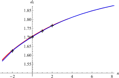
$d_{\rm f}$	$n$	SC	KP17	simulation
LERW	$-2$	$1.6243(10)$	$1.623(6)$	$1.62400(5)$ Wilson2010
SAW	$0$	$1.7027(10)$	$1.7025(7)$	$1.701847(2)$ ClisbyDunweg2016
Ising	$1$	$1.7353(10)$	$1.7352(6)$	$1.7349(65)$ WinterJankeSchakel2008
XY	$2$	$1.7644(10)$	$1.7642(3)$	$1.7655(20)$ ProkofevSvistunov2006 ; WinterJankeSchakel2008

Figure 2: Fractal dimensions of lines in dimension $d=3$. Two expansions are shown: direct (in red) and expansion for $1/d_{\rm f}$ (blue). The table compares our values to results from the literature.

As the insertion of $\frac{1}{2}\int_{y}\sum_{i}\phi_{i}^{2}(y)$ can be generated by deriving the action (7) w.r.t. the mass, the fractal dimension of all lines is related to $\nu$ as in Eq. (21) via

$$d_{\rm f}^{{\rm tot}}=\frac{1}{\nu}=2+\gamma_{1}(g_{*})-\eta\ .$$ (34)

We are now in a position to evaluate the fractal dimension of the blue line, also termed propagator line or backbone, i.e. excluding loops: This is achieved by inserting an operator proportional to $\tilde{\cal E}_{ij}$. To be specific, we consider the insertion of

$$\tilde{\cal E}:=\frac{1}{2}\int_{y}\phi_{1}^{2}(y)-\phi_{2}^{2}(y)\ .$$ (35)

This is, with a normalization convenient for our calculations, the integrated form of $\tilde{\cal E}_{11}-\tilde{\cal E}_{22}$ defined in Eq. (29). When evaluated in a line with index “1” (the correlation function of $\langle\phi_{1}\phi_{1}\rangle$), i.e. in the blue line in Eq. (32) which is connected to the two external points, the result is the same as for the insertion (31). On the other hand, when inserted into a loop (drawn in red), where the sum over indices is unrestricted, it vanishes.

Let us give some background information: In the $O(n)$-model, the number of components $n$ is a priori a positive integer, but can analytically be continued to arbitrary $n$. Two non-positive values of $n$ merit special attention: $n=0$ corresponds to self-avoiding polymers, as shown by De Gennes DeGennes1972 . Here the propagator line (in blue) is interpreted as the self-avoiding polymer, and the red loops are absent. Focusing on lattice configurations with one self-intersection, see Eq. (32), the choice of $g=1$ cancels the free-theory result, giving total weight 0 for self-intersecting paths – as expected. The second case of interest is $n=-2$, and corresponds to loop-erased random walks WieseFedorenko2018 ; WieseFedorenko2019 . Here all perturbative terms $\sim g$ cancel, as the propagator of a loop-erased random walk is identical to that of a random walk. To our advantage, we can equivalently use the cancelation of the first two lines (as for self-avoiding polymers). Then the random walk is redrawn in a way making visible the loop-erased random walk (in blue) and the erased loop (in red), allowing to extract the fractal dimension of the loop-erased random walk via the operator $\tilde{\cal E}$ as given in Eq. (35). For details, we refer to Refs. WieseFedorenko2018 ; WieseFedorenko2019 .

The operator $\tilde{\cal E}$ can be renormalized multiplicatively, by considering the insertion

$$\delta S=\lambda\frac{Z_{\tilde{\cal E}}}{2}\int_{y}\phi_{0,1}^{2}(y)-\phi_{0,2}^{2}(y)\ ,$$ (36)

where $\phi_{0,i}$ denotes the $i$-th component of the bare field $\phi_{0}$. As a result, the fractal dimension of the propagator (or backbone) line is given by

$$d_{\rm f} = 2+\gamma_{\tilde{\cal E}}(g_{*})-\eta\ ,$$ (37)

$$\gamma_{\tilde{\cal E}} := \mu\frac{\partial}{\partial\mu}\ln(Z_{\tilde{\cal E}})=\beta(g)\frac{\partial}{\partial g}\ln(Z_{\tilde{\cal E}}(g))\ .$$ (38)

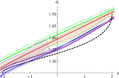
$d_{\rm f}$	$n$	SC	KP17	CFT
LERW	$-2$	$1.244(6)$	$1.188(55)$	$5/4=1.25$
SAW	$0$	$1.354(5)$	$1.350(8)$	$4/3\simeq 1.333$
Ising	$1$	$1.416(1)$	$1.413(7)$	$11/8=1.375$
XY	$2$	$1.482(1)$	$1.480(4)$	$3/2=1.5$

Figure 3: The fractal dimension of lines in dimension $d=2$, as extracted from field theory (colored), and compared to exact results (black dashed line). The different curves are from resummation of $d_{\rm f}$ (blue), $d_{\rm f}^{-1}$ (red), $d_{\rm f}^{2}$ (cyan), and $d_{\rm f}^{-2}$ (green). The table compares the result of our different schemes, with the direct expansion of $d_{\rm f}$ used for SC. Note that the error given is the error of the expansion in one scheme. Comparing different expansion schemes, we estimate the overall error to be of order $0.05$.

The explicit result to 6-loop order is given below in Eq. (II). In the literature Kirkham1981 ; Amit ; Gracey2002 ; ShimadaHikami2016 ; WieseFedorenko2018 one also finds the ratio

$$\phi_{\rm c}(n):=\nu d_{\rm f}\equiv\frac{d_{\rm f}}{d_{\rm f}^{\rm tot}}\equiv\frac{2+\gamma_{\tilde{\cal E}}(g_{*})-\eta}{2+\gamma_{1}(g_{*})-\eta}\ .$$ (39)

It is known as crossover exponent, since it describes the crossover from a broken symmetry $O(k)$, $k<n$, to $O(n)$. We will review this in section IV below. Since for $n=0$ all loops are absent, the two fractal dimensions coincide. For positive $n$, the fractal formed by backbone plus loops is larger than the backbone, and we expect $d_{\rm f}^{\rm tot}>d_{\rm f}$. Translated to $\phi_{\rm c}(n)$ this implies

$$\phi_{\rm c}(0)=1\ ,\qquad\phi_{\rm c}^{\prime}(n)>0\ .$$ (40)

The last relation, which is stronger than $d_{\rm f}^{\rm tot}>d_{\rm f}$ is expected since the derivative w.r.t. $n$ counts loops which are added to the fractal when increasing $n$, which should be positive.

Let us now turn to a comparison of the fractal dimension given by Eq. (37) with numerical simulations. There are four systems for which simulations are available (summarized in Fig. 2).

1. loop-erased random walks: As shown in WieseFedorenko2018 this is given by $n=-2$, in all dimensions.

2. self-avoiding polymers: $n=0$. Here $d_{\rm f}\equiv 1/\nu$.

3. Ising model: $n=1$.

4. XY-model: $n=2$.

Simulations for the Ising and XY model are performed on the lattice ProkofevSvistunov2006 ; WinterJankeSchakel2008 , by considering the high-temperature expansion which allows the authors to distinguish between propagator lines and loops, similar to our discussion of the perturbative expansion (32).

In all cases, the agreement of our RG results with simulations in $d=3$ is excellent, firmly establishing that the appropriate operator was identified. In dimension $d=2$ (shown on Fig. 3), different resummation procedures (see below) yield different results, showing that extrapolations down to $d=2$ are difficult. This can be understood from the non-analytic behavior of the exact result close to $n=\pm 2$. It is even more pronounced for the exponent $\nu$ (see figure 11 below), which diverges with a square-root singularity at $n=2$. We will come back to this issue in section VI.

The remainder of this article is organized as follows: In section II we give the explicit result for the new RG-function $\gamma_{\tilde{\cal E}}$. Section III introduces a self-consistent resummation procedure as a (fast) alternative to the elaborate scheme of Ref. KompanietsPanzer2017 . In the next two sections we discuss in more detail the dimension of curves, and their relation to the crossover exponent (section IV) and loop-erased random walks (section V). Section VI tests the $\epsilon$-expansion against analytic results in dimension $d=2$, allowing us to identify the most suitable variables for the resummation procedure. This allows us to give in section VII improved predictions for all relevant exponents in dimension $d=3$. Section VIII makes the connection to known results from the large-$n$ expansion, which serves as a non-trivial test of our results. We conclude in section IX.

II The RG function $\gamma_{\tilde{\cal E}}$

The RG function $\gamma_{\tilde{\cal E}}$ to 6-loop order, evaluated at the fixed point, reads (with $d=4-\epsilon$)

$$\gamma_{\tilde{\cal E}} = -\frac{2\epsilon}{n+8}+\epsilon^{2}\left[\frac{\left(n^{2}-4n-36\right)}{(n+8)^{3}}\right]+\epsilon^{3}\left[\frac{24(5n+22)\zeta_{3}}{(n+8)^{4}}+\frac{n^{4}+45n^{3}+190n^{2}-144n-1568}{2(n+8)^{5}}\right]$$

$$+ \epsilon^{4}\Bigg{[}-\frac{80\left(2n^{2}+55n+186\right)\zeta_{5}}{(n+8)^{5}}+\frac{18(5n+22)\zeta_{4}}{(n+8)^{4}}-\frac{\left(n^{5}+16n^{4}+808n^{3}+3624n^{2}-6240n-30528\right)\zeta_{3}}{2(n+8)^{6}}$$

$$+\frac{2n^{6}+135n^{5}+3672n^{4}+26568n^{3}+87528n^{2}+123264n+6016}{8(n+8)^{7}}\Bigg{]}$$

$$+ \epsilon^{5}\Bigg{[}\frac{882\left(14n^{2}+189n+526\right)\zeta_{7}}{(n+8)^{6}}-\frac{100\left(2n^{2}+55n+186\right)\zeta_{6}}{(n+8)^{5}}-\frac{4\left(5n^{4}+6n^{3}+3444n^{2}+26824n+46752\right)\zeta_{3}^{2}}{(n+8)^{7}}$$

$$+\frac{\left(895n^{4}+20194n^{3}+73636n^{2}-68712n-403392\right)\zeta_{5}}{(n+8)^{7}}-\frac{3\left(n^{5}+16n^{4}+808n^{3}+3624n^{2}-6240n-30528\right)\zeta_{4}}{8(n+8)^{6}}$$ (41)

$$+\frac{\left(n^{7}-36n^{6}-176n^{5}-35336n^{4}-336080n^{3}-842848n^{2}+394624n+2870528\right)\zeta_{3}}{4(n+8)^{8}}$$

$$+\frac{4n^{8}+367n^{7}+13724n^{6}+275384n^{5}+2162776n^{4}+9337408n^{3}+25225728n^{2}+38978560n+22308864}{32(n+8)^{9}}\Bigg{]}$$

$$+ \epsilon^{6}\Bigg{[}-\frac{64\left(1819n^{3}+97823n^{2}+901051n+2150774\right)\zeta_{9}}{9(n+8)^{7}}-\frac{512\left(n^{3}+65n^{2}+619n+1502\right)\zeta_{3}^{3}}{(n+8)^{7}}$$

$$-\frac{216\left(42n^{3}+2279n^{2}+21282n+50512\right)\zeta_{3,5}}{5(n+8)^{7}}+\frac{9\left(28882n^{3}+780579n^{2}+5963882n+13076112\right)\zeta_{8}}{10(n+8)^{7}}$$

$$-\frac{24\left(59n^{4}+5320n^{3}+62044n^{2}+364256n+790368\right)\zeta_{3}\zeta_{5}}{(n+8)^{8}}$$

$$-\frac{\left(3679n^{5}+605258n^{4}+8044820n^{3}+25012072n^{2}-16957632n-109427520\right)\zeta_{7}}{8(n+8)^{8}}$$

$$-\frac{6\left(5n^{4}+6n^{3}+3444n^{2}+26824n+46752\right)\zeta_{3}\zeta_{4}}{(n+8)^{7}}+\frac{5\left(865n^{4}+19342n^{3}+64708n^{2}-109416n-470976\right)\zeta_{6}}{4(n+8)^{7}}$$

$$+\frac{\left(553n^{6}+9206n^{5}+193932n^{4}+341288n^{3}-11260928n^{2}-64278912n-99677184\right)\zeta_{3}^{2}}{2(n+8)^{9}}$$

$$+\frac{\left(-3n^{8}-104n^{7}-13210n^{6}-100464n^{5}+2802392n^{4}+27327488n^{3}+78105408n^{2}+46518912n-78244864\right)\zeta_{5}}{8(n+8)^{9}}$$

$$+\frac{3\left(n^{7}-36n^{6}-176n^{5}-35336n^{4}-336080n^{3}-842848n^{2}+394624n+2870528\right)\zeta_{4}}{16(n+8)^{8}}$$

$$+\Big{(}n^{9}+100n^{8}+979n^{7}+54758n^{6}-770188n^{5}-15180440n^{4}-80189984n^{3}-169245120n^{2}$$

$$\qquad\qquad\qquad-68332544n+162652160\Big{)}\frac{\zeta_{3}}{8(n+8)^{10}}$$

$$+\Big{(}8n^{10}+927n^{9}+48746n^{8}+1370920n^{7}+22319040n^{6}+172596192n^{5}+774280256n^{4}+2372987392n^{3}$$

$$\qquad\qquad\qquad+5281970176n^{2}+7489404928n+4525309952\Big{)}\frac{1}{128(n+8)^{11}}\Bigg{]}+\mathcal{O}(\epsilon^{7})$$

This agrees with Kirkham Kirkham1981 Eq. (12) up to 4-loop order. The constant $\zeta_{3,5}$ is defined as

$$\zeta_{3,5}:=\sum_{1\leq n<m}\frac{1}{n^{3}m^{5}}\approx 0.037707673\ .$$ (42)

For $n=-2$ to $2$, numerical values of $\gamma_{\tilde{\cal E}}$ and $d_{\rm f}$ are given in table 1.

Table 1: Numerical values for the $6$-loop RG function $\gamma_{\tilde{\cal E}}(\epsilon)$ at the fixed point.

$\quad n\quad$	$\qquad\qquad\qquad\qquad\qquad\qquad\qquad\gamma_{\tilde{\cal E}}(\epsilon)$
$-2$	$-0.333333\epsilon-0.111111\epsilon^{2}+0.211568\epsilon^{3}-0.611186\epsilon^{4}+2.43354\epsilon^{5}-11.7939\epsilon^{6}+\mathcal{O}(\epsilon^{7})$
$-1$	$-0.285714\epsilon-0.090379\epsilon^{2}+0.166245\epsilon^{3}-0.416899\epsilon^{4}+1.50701\epsilon^{5}-6.60415\epsilon^{6}+\mathcal{O}(\epsilon^{7})$
$0$	$-0.25\epsilon-0.0703125\epsilon^{2}+0.131027\epsilon^{3}-0.29588\epsilon^{4}+0.982638\epsilon^{5}-3.94648\epsilon^{6}+\mathcal{O}(\epsilon^{7})$
$1$	$-0.222222\epsilon-0.0534979\epsilon^{2}+0.106224\epsilon^{3}-0.218192\epsilon^{4}+0.673348\epsilon^{5}-2.50444\epsilon^{6}+\mathcal{O}(\epsilon^{7})$
$2$	$-0.2\epsilon-0.04\epsilon^{2}+0.088718\epsilon^{3}-0.165781\epsilon^{4}+0.481055\epsilon^{5}-1.67071\epsilon^{6}+\mathcal{O}(\epsilon^{7})$

Table 2: Numerical values for the $6$-loop fractal dimension $d_{\rm f}(\epsilon)$.

$\quad n\quad$	$\qquad\qquad\qquad\qquad\qquad\qquad\qquad d_{\rm f}(\epsilon)$
$-2$	$2-0.333333\epsilon-0.111111\epsilon^{2}+0.211568\epsilon^{3}-0.611186\epsilon^{4}+2.43354\epsilon^{5}-11.7939\epsilon^{6}+\mathcal{O}(\epsilon^{7})$
$-1$	$2-0.285714\epsilon-0.100583\epsilon^{2}+0.155051\epsilon^{3}-0.410163\epsilon^{4}+1.48492\epsilon^{5}-6.52249\epsilon^{6}+\mathcal{O}(\epsilon^{7})$
$0$	$2-0.25\epsilon-0.0859375\epsilon^{2}+0.114425\epsilon^{3}-0.287513\epsilon^{4}+0.956133\epsilon^{5}-3.85575\epsilon^{6}+\mathcal{O}(\epsilon^{7})$
$1$	$2-0.222222\epsilon-0.0720165\epsilon^{2}+0.0875336\epsilon^{3}-0.209864\epsilon^{4}+0.647691\epsilon^{5}-2.42316\epsilon^{6}+\mathcal{O}(\epsilon^{7})$
$2$	$2-0.2\epsilon-0.06\epsilon^{2}+0.069718\epsilon^{3}-0.157887\epsilon^{4}+0.457846\epsilon^{5}-1.60209\epsilon^{6}+\mathcal{O}(\epsilon^{7})$

III A self-consistent resummation procedure

Figure 4: The ratios $r_{n}$ as given in Eq. (45) for $\alpha=0$, and the fit to Eq. (46).

Figure 5: Resummation of $d_{\rm f}$ for LERWs ($n=-2$) in $d=3$, as a function of the series-order $n$, setting $\alpha=0$. One sees that the resummed series converges, for all assumed values of the branch cut, with orange $z_{\rm bc}=0.3/a$ to green with $z_{{\rm bc}}=1/a$, ending with cyan $z_{{\rm bc}}=1.1/a$, which clearly sits inside the supposed branch cut, which oscillates, and for which only the real part is shown.

Figure 6: Minus the exponential decay constant $c$ from Eq. (46).

There are many resummation procedures GuidaZinn-Justin1998 ; Kleinert2000 ; we show results based on the Borel-resummation method proposed in Ref. KompanietsPanzer2017 and denoted KP17. We also propose a different approach, using a self-consistent (SC) resummation: Consider an exponent or observable $\kappa(\epsilon)$, with series expansion

$$\kappa(\epsilon)=\sum_{n=0}^{\infty}b_{n}\epsilon^{n}\ .$$ (43)

Suppose that $b_{n}$ has the asymptotic form

$$b_{n}=c_{0}a^{n}n!n^{\alpha}\ .$$ (44)

Then

$$r_{n}:=\frac{b_{n}}{b_{n-1}}\frac{1}{n}\left(\frac{n}{n-1}\right)^{\alpha}=a+\delta a(n)\ .$$ (45)

Further suppose that, with $c>0$

$$\delta a(n)=b\,\mathrm{e}^{-cn}\ .$$ (46)

This ansatz can be used to fit the last three elements of the table of $r_{n}$ (at 6-loop order this is $r_{2},...,r_{6}$) to the three parameters $a$, $b$, and $c$. The value of $a$ is our best estimate for the inverse of the branch-cut location in the inverse Borel transform. Having established a fit allows us to estimate the ratios $r_{i}$ with $i$ larger than the order to which we calculated. It in turn fixes $b_{n}$ to the same order, in practice up to order $28...40$ using double precision, and depending on the series. An example studying the fractal dimension of LERWs is given on Figs. 4 and 5, for $\alpha=0$. In general, the fit (46) is possible only for a certain range of $\alpha$. The fit fails if the three chosen ratios $r_{n}$ are not monotone, as the exponential function then grows. As a consequence, in this case the SC scheme makes no prediction, and we leave the corresponding table entries empty. Different fitting forms could be proposed and tested, e.g. to account for such a non-monotone behavior. We restricted our tests to an algebraic decay, but no benefit could be extracted from the latter. We believe that the advantage of the ansatz (45) is its fast convergence, which is lost for an ansatz with algebraic decay.

We can still use our freedom to choose $\alpha$, which also leads to different values of the exponential decay $c$ given in Fig. 6. Our approach is to try with all values of $\alpha$ for which a fit of the form (46) is feasible. The result is shown on Fig. 7: Apart from error bars of the procedure, we obtain the mid-range and the mean of all obtained exponents as the centered and best estimates. Note that when the allowed range of $\alpha$ is small, the estimated error bars are also small, since the estimate varies continuously with $\alpha$. Thus a small error bar may indicate a robust series and indeed a small error, or a series which is delicate to resum. As a consequence, error bars of this method have to be taken with a grain of salt. The method of KP17 KompanietsPanzer2017 does not suffer from this artifact.

IV Dimension of curves and Crossover Exponent

Table 3: Numerical values for the $6$-loop $\phi^{\prime}_{c}(0)$ .

$\quad d\quad$	SC	KP17	exact
$0$	$0.70(18)$	$-$
$1$	$0.44(6)$	$\quad 0.58(12)$
$2$	$0.239(10)$	$\quad 0.262(10)$	$\displaystyle\frac{3}{4\pi}\simeq 0.238732$
$3$	$0.0912(7)$	$\quad 0.0925(4)$
$4$	0	0	0

Following the classic book by Amit Amit , (for more references see Kirkham1981 ; KiskisNarayananVranas1993 ; ShimadaHikami2016 ) the crossover exponent arises for the following question: Consider the anisotropic $O(n)$ model, where the first $k<n$ components have a mass $m_{1}^{2}$, and the remaining $n-k$ components have a mass $m_{2}^{2}$ (we suppressed the index 0 for the bare objects for convenience of notation)

$${{\cal S}} = \int_{x}\,\frac{m^{2}_{1}}{2}\sum_{i=1}^{k}\phi_{i}(x)^{2}+\frac{m^{2}_{2}}{2}\sum_{i=k+1}^{n}\phi_{i}(x)^{2}+\frac{1}{2}[\nabla\vec{\phi}(x)]^{2}$$ (47)

$$\quad+\frac{16\pi^{2}}{4!}g\!\left[\vec{\phi}(x)^{2}\right]^{2}\ .$$

This form arises in mean-field theory, when coarse graining a $n$-component model with anisotropy. Consider $m_{1}^{2}<m_{2}^{2}$, i.e. $\lambda:=m_{2}^{2}-m_{1}^{2}>0$. The corresponding phase diagram is shown on figure 9. When lowering the temperature, the $k$ first modes will become massless before the remaining ones, and one arrives at an effective $O(k)$ model. In the opposite case, $m_{1}^{2}>m_{2}^{2}$, the remaining $n-k$ modes become massless first, resulting in a critical $O(n-k)$ model, while for $m_{1}^{2}=m_{2}^{2}$ all modes becomes massless at the same temperature.

Let us rewrite the quadratic (derivative free) terms in Eq. (47) as

$${{\cal S}_{m^{2}}}=\frac{m^{2}}{2}\vec{\phi}(x)^{2}-\frac{\lambda}{2}\tilde{\cal E}\ ,$$ (48)

where

$$m^{2} := \frac{km_{1}^{2}+(n-k)m_{2}^{2}}{n}\ ,$$ (49)

$$\lambda := m_{2}^{2}-m_{1}^{2}\ ,$$ (50)

$$\tilde{\cal E} = \frac{1}{n}\left[(n-k)\sum_{i=1}^{k}\phi_{i}(x)^{2}-k\sum_{i=k+1}^{n}\phi_{i}(x)^{2}\right]\ .\qquad$$ (51)

Further denote the distance to the critical point by

$$t:=\frac{T-T_{{\rm c},n}}{T_{{\rm c},n}}\ .$$ (52)

Then any thermodynamic observable, as e.g. the longitudinal susceptibility, will assume a scaling form with $t$ as

$$\chi_{L}^{-1}(t,g)=t^{\gamma}f\left(\frac{\lambda}{t^{\phi_{\rm c}}}\right)\ .$$ (53)

The function $f$ is the crossover function, while $\phi_{\rm c}$ is the crossover exponent. It is the ratio of dimensions between $\lambda$ and $m^{2}$, namely

$$\phi_{\rm c}=\frac{\mbox{dim}_{\mu}(\lambda)}{\mbox{dim}_{\mu}(m^{2})}=\frac{2+\gamma_{\tilde{\cal E}}(g_{*})-\eta}{2+\gamma_{1}(g_{*})-\eta}\ .$$ (54)

In the numerator is the renormalization of $\tilde{\cal E}$ as given by Eq. (51), and which sits in the same representation as $\tilde{\cal E}_{{i,j}}$ defined in Eq. (29) or $\tilde{\cal E}$ defined in Eq. (35) (thus the same notation for all these objects), and which is the fractal dimen- sion $d_{{\rm f}}$ of the backbone, as given in Eq. (37) . The denominator is $\nu^{-1}=d_{\rm f}^{\rm tot}$, as introduced in Eq. (19). This allows us to rewrite $\phi_{c}$ as in Eq. (39) as

$$\phi_{\rm c}=\frac{d_{\rm f}}{d_{\rm f}^{\rm tot}}=\nu d_{\rm f}\ .$$ (55)

Its series expansion reads

$$\phi_{\rm c} = 1+\frac{\epsilon n}{2(n+8)}+\frac{\epsilon^{2}n\left(n^{2}+24n+68\right)}{4(n+8)^{3}}+\epsilon^{3}\bigg{[}-\frac{6n(5n+22)\zeta_{3}}{(n+8)^{4}}+\frac{n\left(n^{4}+48n^{3}+788n^{2}+3472n+5024\right)}{8(n+8)^{5}}\bigg{]}$$

$$+ \epsilon^{4}\bigg{[}\frac{20n\left(2n^{2}+55n+186\right)\zeta_{5}}{(n+8)^{5}}-\frac{9n(5n+22)\zeta_{4}}{2(n+8)^{4}}-\frac{n\left(n^{4}-13n^{3}+544n^{2}+4716n+8360\right)\zeta_{3}}{(n+8)^{6}}$$

$$+\frac{n\left(n^{6}+72n^{5}+2085n^{4}+28412n^{3}+147108n^{2}+337152n+306240\right)}{16(n+8)^{7}}\bigg{]}$$

$$+ \epsilon^{5}\bigg{[}-\frac{441n\left(14n^{2}+189n+526\right)\zeta_{7}}{2(n+8)^{6}}+\frac{25n\left(2n^{2}+55n+186\right)\zeta_{6}}{(n+8)^{5}}+\frac{2n\left(4n^{4}+39n^{3}+2028n^{2}+14468n+24528\right)\zeta_{3}^{2}}{(n+8)^{7}}$$ (56)

$$+\frac{n\left(-230n^{4}-2857n^{3}+33832n^{2}+280596n+466016\right)\zeta_{5}}{2(n+8)^{7}}-\frac{3n\left(n^{4}-13n^{3}+544n^{2}+4716n+8360\right)\zeta_{4}}{4(n+8)^{6}}$$

$$-\frac{n\left(9n^{5}-661n^{4}+7584n^{3}+125232n^{2}+465592n+554064\right)\zeta_{3}}{(n+8)^{8}}$$

$$+\frac{n\left(n^{8}+96n^{7}+4154n^{6}+95668n^{5}+1177480n^{4}+6723904n^{3}+19390624n^{2}+28388096n+17677824\right)}{32(n+8)^{9}}\bigg{]}$$

$$+ \epsilon^{6}\bigg{[}\frac{16n\left(1819n^{3}+97823n^{2}+901051n+2150774\right)\zeta_{9}}{9(n+8)^{7}}+\frac{128n\left(n^{3}+65n^{2}+619n+1502\right)\zeta_{3}^{3}}{(n+8)^{7}}$$

$$-\frac{9n\left(28882n^{3}+780579n^{2}+5963882n+13076112\right)\zeta_{8}}{40(n+8)^{7}}+\frac{54n\left(42n^{3}+2279n^{2}+21282n+50512\right)\zeta_{3,5}}{5(n+8)^{7}}$$

$$+\frac{12n\left(13n^{4}+2288n^{3}+28088n^{2}+172816n+385584\right)\zeta_{3}\zeta_{5}}{(n+8)^{8}}$$

$$+\frac{n\left(1136n^{5}+174529n^{4}+1284304n^{3}-8699596n^{2}-73803936n-120419232\right)\zeta_{7}}{16(n+8)^{8}}$$

$${+}\frac{3n\left(4n^{4}+39n^{3}+2028n^{2}+14468n+24528\right)\zeta_{3}\zeta_{4}}{(n+8)^{7}}$$

$$-\frac{5n\left(215n^{4}+2431n^{3}-38296n^{2}-300948n-499808\right)\zeta_{6}}{8(n+8)^{7}}$$

$$+\frac{n\left(-140n^{6}-471n^{5}-2192n^{4}+947100n^{3}+11661984n^{2}+46428608n+61839872\right)\zeta_{3}^{2}}{4(n+8)^{9}}$$

$$+\frac{n\left(-6n^{7}+348n^{6}-30199n^{5}-656384n^{4}-615916n^{3}+21367744n^{2}+87069536n+100818688\right)\zeta_{5}}{8(n+8)^{9}}$$

$$-\frac{3n\left(9n^{5}-661n^{4}+7584n^{3}+125232n^{2}+465592n+554064\right)\zeta_{4}}{4(n+8)^{8}}$$

$$+\frac{n\left(2n^{8}-19n^{7}+689n^{6}+168914n^{5}-416016n^{4}-21086984n^{3}-121746544n^{2}-283766528n-249483264\right)\zeta_{3}}{8(n+8)^{10}}$$

$$+\Big{(}4n^{10}+480n^{9}+27419n^{8}+921208n^{7}+18509364n^{6}+215607792n^{5}+1332297632n^{4}+4570604800n^{3}$$

$$+8857566208n^{2}+9208365056n+4150108160\Big{)}\frac{n}{256(n+8)^{11}}\bigg{]}+\mathcal{O}(\epsilon^{7})\ .$$

(a)

(b)

Figure 7: (a): In blue the fractal dimension $d_{\rm f}$ of LERWs as a function of $\alpha$. The latter yields bounds for $d_{\rm f}$, i.e. $d_{\rm f}\in[1.62378,1.6254]$, and as a best estimate the mean of the obtained values, $d_{\rm f}\approx 1.62426$ (blue dashed line). The numerical result is $d_{\rm f}=1.62400\pm 0.00005$ (orange with error bars in dashes). Wilson2010 . (b): same for $d=2$. We find $d_{\rm f}\in[1.238,1.259]$, with a mean estimate $d_{\rm f}=1.244$, to be compared to the exact result $d_{\rm f}=5/4$. Using only the 5-loop series gives $d_{\rm f}(d=3)\approx 1.621$, and $d_{\rm f}(d=2)=1.11.$

Figure 8: The crossover phase diagram as given by Amit , with $\lambda=m_{2}^{2}-m_{1}^{2}$. The thick black line is a line of first-order phase transitions. Figure 9: Slope of the crossover exponent at $n=0$ for dimensions $0\leq d\leq 4$. The black cross is the analytic result from Eq. (102) in $d=2$.

This agrees with Kirkham1981 Eq. (14) for $\phi_{\rm c}$ (noted $\phi$ there), except for a misprint for the order $\epsilon^{3}$ term: the coefficient $682$ in the second line of Eq. (14) of Kirkham1981 should read $628$.

The curve $\phi_{\rm c}(n)$, at least in higher dimensions is rather straight, thus the most important quantity to give is

$$\phi_{c}^{\prime}(0)|_{d=0} = 0.70(18)$$ (57)

$$\phi_{c}^{\prime}(0)|_{d=1} = 0.44(6)$$ (58)

$$\phi_{c}^{\prime}(0)|_{d=2} = 0.239(10)$$ (59)

$$\phi_{c}^{\prime}(0)|_{d=3} = 0.0912(7)\ .$$ (60)

We have in all dimensions $d$

$$\phi_{c}^{\prime}(0)=\nu\left[\gamma_{\tilde{\cal E}}^{\prime}(0)-\gamma_{1}^{\prime}(0)\right]\ .$$ (61)

Estimates for $\phi_{c}^{\prime}(0)$ obtained by self-consistent resummation (SC) and the procedure suggested in KompanietsPanzer2017 (KP17) are presented in table 3 and Fig. 9. Integrals of the inverse Borel transform do not converge well for $d=0$ in the KP17 resummation scheme, which prevents us to obtain an estimate there.

Explicit values for the crossover exponent in $d=3$ to be compared with experiments, high-temperature series expansion and numerics are

$$\phi_{\rm c}^{\rm SC}(d=3,n=1) = 1.089(1)\$$ (62)

$$\phi_{\rm c}^{\rm SC}(d=3,n=2) = 1.180(4)\$$ (63)

$$\phi_{\rm c}^{\rm SC}(d=3,n=3) = 1.265(5)\$$ (64)

$$\phi_{\rm c}^{\rm SC}(d=3,n=4) = 1.329(8)\$$ (65)

$$\phi_{\rm c}^{\rm SC}(d=3,n=5) = 1.391(2)\ .$$ (66)

There are experiments for $n=2$ and $n=3$. For $n=2$:

$$\phi_{\rm c}^{\rm exp}(d=3,n=2) = 1.17(2)~{}~{}~{}\mbox{ \cite[cite]{\@@bibref{Authors Phrase1YearPhrase2}{RohrerGerber1977}{\@@citephrase{(}}{\@@citephrase{)}}}}$$ (67)

$$\phi_{\rm c}^{\rm exp}(d=3,n=2) = 1.18(5)~{}~{}~{}\mbox{ \cite[cite]{\@@bibref{Authors Phrase1YearPhrase2}{Domann1979}{\@@citephrase{(}}{\@@citephrase{)}}}}$$ (68)

$$\phi_{\rm c}^{\rm exp}(d=3,n=2) = 1.23(4)~{}~{}~{}\mbox{ \cite[cite]{\@@bibref{Authors Phrase1YearPhrase2}{MajkrzakAxeBruce1980}{\@@citephrase{(}}{\@@citephrase{)}}}}$$ (69)

$$\phi_{\rm c}^{\rm exp}(d=3,n=2) = 1.19(3)~{}~{}~{}\mbox{ \cite[cite]{\@@bibref{Authors Phrase1YearPhrase2}{WalischPerez-MatoPetersson1989}{\@@citephrase{(}}{\@@citephrase{)}}}}$$ (70)

$$\phi_{\rm c}^{\rm exp}(d=3,n=2) = 1.17(10)~{}\mbox{ \cite[cite]{\@@bibref{Authors Phrase1YearPhrase2}{WuYoungShaoGarlandBirgeneauHeppke1994}{\@@citephrase{(}}{\@@citephrase{)}}}}\ .$$ (71)

The first paper RohrerGerber1977 examines the bicritical point in GdAl$\mathrm{O}_{3}$, and the second one Domann1979 the bicritical point in TbP$\mathrm{O}_{4}$. In the third MajkrzakAxeBruce1980 the structural phase transition in K₂SeO₄ is investigated. The fourth one WalischPerez-MatoPetersson1989 is related to a continuous phase transition in Rb₂ZnCl₄. The last one is for the nematic-smectic-A₂ transition WuYoungShaoGarlandBirgeneauHeppke1994 .

Let us proceed to $n=3$:

$$\phi_{\rm c}^{\rm exp}(d=3,n=3) = 1.278(26)~{}\mbox{ \cite[cite]{\@@bibref{Authors Phrase1YearPhrase2}{ShapiraOliveira1978}{\@@citephrase{(}}{\@@citephrase{)}}}}$$ (72)

$$\phi_{\rm c}^{\rm exp}(d=3,n=3) = 1.274(45)~{}\mbox{ \cite[cite]{\@@bibref{Authors Phrase1YearPhrase2}{ShapiraOliveira1978}{\@@citephrase{(}}{\@@citephrase{)}}}}$$ (73)

$$\phi_{\rm c}^{\rm exp}(d=3,n=3) = 1.279(31)~{}\mbox{ \cite[cite]{\@@bibref{Authors Phrase1YearPhrase2}{KingRohrer1979}{\@@citephrase{(}}{\@@citephrase{)}}}}\ .$$ (74)

The first two figures are for two different samples of the very nearly isotropic antiferromagnet RbMnF₃ ShapiraOliveira1978 , the last one KingRohrer1979 is for the bicritical point in MnF₂.

In Ref. Zhang1997 a theory based on ${\rm SO}(5)$, i.e. $n=5$, has been proposed to explain superconductivity and antiferromagnetism in a unified model. While MC simulations support this scenario Hu2001 ; Hu2002 , it has been argued in Ref. Aharony2002 that the isotropic fixed point is unstable and breaks down into ${\rm SO}(2)\times{\rm SO}(3)$.

Recent Monte Carlo simulations HasenbuschVicari2011 provide very precise estimates for the crossover exponent for $n=2,3,4$ (in terms of HasenbuschVicari2011 $\phi_{c}=Y_{2}\nu$):

$$\phi_{\rm c}^{\rm MC}(d=3,n=2) = 1.1848(8)$$ (75)

$$\phi_{\rm c}^{\rm MC}(d=3,n=3) = 1.2735(9)$$ (76)

$$\phi_{\rm c}^{\rm MC}(d=3,n=4) = 1.3567(15)$$ (77)

The high-temperature series expansion of PfeutyJasnowFisher1974 yields

$$\phi_{\rm c}^{\rm HT}(d=3,n=2) = 1.175(15)\ ,$$ (78)

$$\phi_{\rm c}^{\rm HT}(d=3,n=3) = 1.250(15)\ .$$ (79)

An alternative to the $\epsilon$-expansion is to work directly in dimension $d=3$, (renormalization group in fixed space dimension $d=3$, denoted RG3), as was done in Ref. CalabresePelissettoVicari2002 :

$$\phi_{c}^{\rm RG3}(n=2) = 1.184(12)$$ (80)

$$\phi_{\rm c}^{\rm RG3}(n=3) = 1.271(21)$$ (81)

$$\phi_{\rm c}^{\rm RG3}(n=4) = 1.35(4)$$ (82)

$$\phi_{\rm c}^{\rm RG3}(n=5) = 1.40(4)$$ (83)

$$\phi_{\rm c}^{\rm RG3}(n=8) = 1.55(4)$$ (84)

$$\phi_{\rm c}^{\rm RG3}(n=16) = 1.75(6)\ .$$ (85)

Another approach is the non-perturbative renormalization group (NPRG). With this method the following estimates were obtained EichhornMesterhazyScherer2013 (in terms of EichhornMesterhazyScherer2013 $\phi_{\rm c}=\theta_{1}/\theta_{2}=y_{2,2}\nu$):

$$\phi_{\rm c}^{\rm NPRG}(n=2) = 1.209$$ (86)

$$\phi_{\rm c}^{\rm NPRG}(n=3) = 1.314$$ (87)

$$\phi_{\rm c}^{\rm NPRG}(n=4) = 1.407$$ (88)

$$\phi_{\rm c}^{\rm NPRG}(n=5) = 1.485$$ (89)

$$\phi_{\rm c}^{\rm NPRG}(n=10) = 1.710\ .$$ (90)

Values provided by NPRG are systematically higher than those provided by other methods, but it is not clear how precise these values are. Their deviation from all other values is on the level of several percent, and we believe this to be an appropriate error estimate.

Table 4: Numerical values for $\phi_{c}(n)$ in $d=3$.

$\quad n\quad$	SC	SC from $\phi_{\rm c}^{-13/4}$	KP17	KP17 $\phi_{\rm c}^{-13/4}$	RG3 CalabresePelissettoVicari2002	NPRG EichhornMesterhazyScherer2013	HT PfeutyJasnowFisher1974	MC HasenbuschVicari2011	experiment
$2$	$1.180(4)$	1.183(1)	$1.183(3)$	1.1843(6)	$1.184(12)$	1.209	$1.175(15)$	$1.1848(8)$	$1.17(2)$  RohrerGerber1977
									$1.18(5)$  Domann1979
									$1.19(3)$  WalischPerez-MatoPetersson1989
									$1.23(4)$  MajkrzakAxeBruce1980
									$1.17(10)$ WuYoungShaoGarlandBirgeneauHeppke1994
$3$	$1.265(5)$	1.273(1)	$1.263(13)$	1.2742(10)	1.271(21)	1.314	$1.250(15)$	$1.2735(9)$	$1.278(26)$ ShapiraOliveira1978
									$1.274(45)$ ShapiraOliveira1978
									$1.279(31)$ KingRohrer1979
$4$	1.329(5)	1.361(1)	$1.33(3)$	1.3610(7)	$1.35(4)$	1.407		$1.3567(15)$
$5$	1.391(2)	1.442(2)	$1.42(4)$	1.444(5)	$1.40(4)$	1.485
$8$	1.534(2)	1.64(1)	$1.59(7)$	1.625(17)	$1.55(4)$

The most precise 6-loop estimates are obtained by a resummation of the $\phi_{\rm c}^{-13/4}$ expansion: they have lower error estimates (in both the S.C. and KP17 method) and better agree with the most precise values from Monte Carlo simulations. See also discussion in Sec. VI.2.

A summary is provided in table 4.

V Loop-erased random walks

Figure 10: $d_{\rm f}$ as a function of $d$ for LERW ($n=-2$). The red dashed line is the bound $d_{\rm f}\leq\frac{5}{6-d}$ SapozhnikovShiraishi2018 (bound continuation to all dimensions guessed). The gray dashed lines are the bounds $1\leq d_{\rm f}\leq d_{{\rm RW}}=2$.

The connection between the $O(n)$-symmetric $\phi^{4}$-theory at $n=-2$ and loop-erased random walks has only recently been established for all dimensions $d$ WieseFedorenko2018 , even though in $d=2$ this was known from integrability Nienhuis1982 ; Duplantier1992 . As we discussed above (see after Eq. (21)), this is a random walk where loops are erased as soon as they are formed. As such it is a non-Markovian process. On the other hand, its trace is equivalent to that of the Laplacian Random Walk LyklemaEvertszPietronero1986 ; Lawler2006 , which is Markovian, if one considers the whole trace as state variable. It is constructed on the lattice by solving the Laplace equation $\nabla^{2}\Phi(x)=0$ with boundary conditions $\Phi(x)=0$ on the already constructed curve, while $\Phi(x)=1$ at the destination of the walk, either a chosen point, or infinity. The walk then advances from its tip $x$ to a neighboring point $y$, with probability proportional to $\Phi(y)$. In dimension $d=2$, it is known via the relation to stochastic Löwner evolution (SLE) LawlerSchrammWerner2004 ; Cardy2005 that the fractal dimension of LERWs is

$$d^{\rm LERW}_{\rm f}(d=2)=\frac{5}{4}\ .$$ (91)

(a)

(b)

Figure 11: The exponent $\nu$ for $d=2$ (a) and its inverse (b). The different colors come from resummations of $\nu$ (blue), $1/\nu$ (red), $1/\nu^{2}$ (green), $1/\nu^{3}$ (cyan), and $\alpha=2-\nu d$ (dark green). The dashed black line is from CFT as given by Eq. (100). The shaded errors are (minimal) errors estimated from the uncertainty in the extrapolation, see section III.

In three dimensions, there is no analytic prediction for the fractal dimension of LERWs, only the bound SapozhnikovShiraishi2018

$$1\leq d_{\rm f}^{{\rm LERW}}\leq\frac{5}{3}\ .$$ (92)

We conjecture that it can be generalized to arbitrary dimension $d$ as

$$1\leq d_{\rm f}^{{\rm LERW}}\leq\frac{5}{6-d}\ .$$ (93)

Note that this conjecture becomes exact in dimensions $d=1$ and $d=2$. The best numerical estimation in $d=3$ is due to D. Wilson Wilson2010

$${d}_{\rm f,num}^{\rm LERW}(d=3)=1.62400\pm 0.00005=1.62400(5)\ .$$ (94)

Our resummations from the field theory are (see Fig. 10)

$$d_{\rm f,SC}^{\rm LERW}(d=3) = 1.6243(10)\ .$$

$$d_{\rm f,KP17}^{\rm LERW}(d=3) = 1.623(6)\ .$$ (95)

VI The limit of $d=2$ checked against conformal field theory

VI.1 Relations from CFT

In $d=2$, all critical exponents should be accessible via conformal field theory (CFT). The latter is based on ideas proposed in the 80s by Belavin, Polyakov and Zamolodchikov BelavinPolyakovZamolodchikov1984 . They constructed a series of minimal models, indexed by an integer $m\geq 3$, starting with the Ising model at $m=3$. These models are conformally invariant and unitary, equivalent to reflection positive in Euclidean theories. For details, see one of the many excellent textbooks on CFT DotsenkoCFT ; DiFrancescoMathieuSenechal ; ItzyksonDrouffe2 ; HenkelCFT . Their conformal charge is given by

$$c=1-\frac{6}{m(m+1)}\ .$$ (96)

The list of conformal dimensions allowed for a given $m$ is given by the Kac formula with integers $r,s$ (Eq. (7.112) of DiFrancescoMathieuSenechal )

$$h_{r,s}=\frac{[r(m+1)-sm]^{2}-1}{4m(m+1)},\ 1\leq r<m,1\leq s\leq m.$$ (97)

It was later realized that other values of $m$ also correspond to physical systems, in particular $m=1$ (loop-erased random walks), and $m=2$ (self-avoiding walks). These values can further be extended to the $\mathcal{O}(n)$-model with non-integer $n$ and $m$, using the identification

$$n=2\cos\left(\frac{\pi}{m}\right)\ .$$ (98)

More strikingly, the table of dimensions allowed by Eq. (97) has to be extended to half-integer values, including $0$. It is instructive to read JankeSchakel2010 , where all operators were identified. This yields the fractal dimension of the propagator line RushkinBettelheimGruzbergWiegmann2007 ; BloeteKnopsNienhuis1992 ; JankeSchakel2010

$$d_{\rm f}=2-2h_{1,0}=1+\frac{\pi}{2\left(\arccos\left(\frac{n}{2}\right)+\pi\right)}\ .$$ (99)

This is compared to the $\epsilon$-expansion on Fig. 3.

For $\nu$, i.e. the inverse fractal dimension of all lines, be it propagator or loops, we get

$$\nu=\frac{1}{2-2h_{1,3}}=\frac{1}{4}\left(1+\frac{\pi}{\arccos(\frac{n}{2})}\right)\ .$$ (100)

This agrees with JankeSchakel2010 , inline after Eq. (2). (Note that the choice $h_{2,1}$ coinciding with $h_{1,3}$ for Ising does nor work for general $n$.) A comparison to the $\epsilon$-expansion is given on Fig. 11.

For $\eta$, there are two suggestive candidates from the Ising model, $\eta=4h_{1,2}=4h_{2,2}$. This does not work for other values of $n$. We propose in agreement with RushkinBettelheimGruzbergWiegmann2007 ; BloeteKnopsNienhuis1992 ; JankeSchakel2010

$$\eta=4h_{\frac{1}{2},0}=\frac{5}{4}-\frac{3\arccos\left(\frac{n}{2}\right)}{4\pi}-\frac{\pi}{\arccos\left(\frac{n}{2}\right)+\pi}\ .$$ (101)

It has a square-root singularity both for $n=-2$ and $n=2$. A comparison to field theory is given on Fig. 12.

As we discuss in the next section, we have no clear candidate for the exponent $\omega$. This is apparent on Fig. 13, where our estimates from the resummation are confronted to some guesses from CFT.

Finally the crossover exponent $\phi_{\rm c}$ defined in Eqs. (39) and (54) becomes

$$\phi_{\rm c}=\nu d_{\rm f}=\frac{1-h_{1,0}}{1-h_{1,3}}=\frac{1}{4}+\frac{3\pi}{8\arccos(\frac{n}{2})}\ .$$ (102)

This is compared to the $\epsilon$-expansion on Fig. 14.

VI.2 Resummation

Figure 12: The exponent $\eta$ in $d=2$. The blue curve is the direct expansion, the green one a resummation of $\sqrt{\eta}$, which, as $\eta$ starts at order $\epsilon^{2}$, has a regular series expansion in $\epsilon$. The black solid line is $\eta=4h_{1/2,0}$ as given by Eq. (101).

Note that there are singularities at $n=\pm 2$, the most severe one being the one at $n=2$ for the exponent $\nu$. For this reason, resummation is difficult for $n\approx 2$. We found that the singularity in $d=2$ is much better reproduced when resumming $1/\nu^{3}$ instead of $\nu$, see Fig. 11. This expansion catches the divergence at $n=2$ in $d=2$, even though the singularity thus constructed is not proportional to $1/\sqrt{2-n}$, but proportional to $1/\sqrt[3]{2-n}$. As we will see below, reproducing this singularity at least approximately renders expansions also more precise in $d=3$, even for $n=0,1$.

The same situation appears for $\phi_{\rm c}$, where $1/\phi_{\rm c}^{13/4}$ provides the most precise fit of the $n=2$ singularity (see Fig. 14). This leads to smaller error bars for both resummation methods (see Table  4) and supports our statement about the necessity of a proper choice of the object for resummation, based on the knowledge of the $d=2$ singularities.

For $d_{\rm f}$ (Fig. 3) and $\eta$ (Fig. 12), the $\epsilon$-expansion is approximately correct. But there are square-root singularities when approaching $n=\pm 2$ in $d=2$, which are not visible in the $\epsilon$-expansion. It is suggestive that these singularities in $d=2$ influence the convergence in $d=3$. Building in these exact results in $d=2$, including the type of singularity in the $(d,n)$-plane would increase significantly the precision in $d=3$.

As for $\omega$ presented on Fig. 13, the situation is rather unclear, as there is no choice of ${h_{r,s}}$ which is a good candidate for all $n$ in the range of $-2\leq n\leq 2$. Intersections in high-temperature graphs are given by $h_{2,0}$, and this operator is the closest in spirit to the $(\vec{\phi}^{2})^{2}$-interaction of our field theory, resulting into

$$\omega_{\rm guess}=2h_{2,0}-2\ .$$ (103)

This contradicts the results from the $\epsilon$-expansion presented on Fig. 13.

Figure 13: The exponent $\omega$ in $d=2$. Dots represent values reported in the literature, mostly based on CFT. The value $\omega=7/4$ for $n=1$ is consistent with the $O(1)$-term in BarouchMcCoyWu1973 , while the reanalysis of CalabreseCaselleCeliPelissettoVicari2000 concludes on $\omega=2$. CalabreseCaselleCeliPelissettoVicari2000 also argue that $\omega=2$ for $n>2$. The black dashed line is the guess (103) resulting from the operator generating an intersection between two lines.

It is not even clear whether this is a question which can be answered via CFT: As all observables depend on the coupling $g$, the exponent $\omega$ quantifies how far this coupling has flown to the IR fixed point. On the other hand, in a CFT the ratio of size $L$ over lattice cutoff $a$ has gone to infinity, and the theory by construction is at $g=g_{*}$. Our results are consistent with $\omega=2$ for all $n$, in which case the associated operator might simply be the determinant of the stress-energy tensor, sometimes (abusively) referred to as $T\bar{T}$, see e.g.  Cardy2018 .

Figure 14: The exponent $\phi_{\rm c}$ in $d=2$. The dashed black line is the analytic result from Eq. (102). The colored lines are resummations of $\phi_{\rm c}$ (blue), $1/\phi_{\rm c}$ (red), $1/\phi_{\rm c}^{2}$ (green), $1/\phi_{\rm c}^{3}$ (cyan), $1/\phi_{\rm c}^{13/4}$ (magenta), and $1/\phi_{\rm c}^{3}$ (gray). Resumming $1/\phi_{\rm c}^{13/4}$ considerably improves the precision.

Figure 15: The exponent $\eta$ in $d=3$. The SC resummation scheme (in blue) seems to be systematically smaller than the values of KP17 (in red). SC resummation of $\sqrt{\eta}$ (in cyan) works slightly better. Black crosses represent the best values from MC and conformal bootstrap, as given in KompanietsPanzer2017 . Figure 16: The exponent $\nu$ in $d=3$, obtained from a resummation of $1/\nu^{3}$. In blue the results from SC, in red using KP17. Black crosses are from MC and conformal bootstrap, as given in KompanietsPanzer2017 .          Figure 17: The exponent $\omega$ in $d=3$ via SC (blue, with shaded error bars), and KP17 (in red). Crosses represent the best values from MC, as given in Ref. KompanietsPanzer2017 . Figure 18: The exponent $\phi_{\rm c}$ in $d=3$. Crosses are from MC and experiments Domann1979 ; ShapiraOliveira1978 . The value for $n=-2$ is taken as $d_{\rm f}/2$ with $d_{\rm f}$ the fractal dimension of LERWs Wilson2010 .

VII Improved estimates in $d=3$ for all exponents

With the knowledge gained in $d=2$, we are now in a position to give our best estimates for all critical exponents. For the exponent $\nu$, we use the expansion of $1/\nu^{3}$, while for $\eta$ and $\omega$ we use the standard direct expansions. For $d_{\rm f}$ we both use the direct expansion, as the expansion of $1/d_{\rm f}$, to get an idea about the errors induced by changing the quantity to be extrapolated.

Our findings are given on Tables 4 to 7 as well as Figs. 2 and 18 to 18. Let us summarize them:

The exponent $\eta$ is shown on Table 5 and figure 18. For SAWs, the agreement of KP17 with the Monte-Carlo results of Clisby2017 ; ClisbyDunweg2016 is better than $10^{-3}$ (relative). For the Ising model ($n=1$), the agreement with the conformal bootstrap KosPolandSimmons-DuffinVichi2016 is of the same order.

Our predictions for $\nu$ are given on table 6 and Fig. 18. Using the expansion of $1/\nu^{3}$, the relative deviation to the conformal bootstrap is about $3\times 10^{-4}$ instead of $10^{-3}$ for the direct expansion, validating both schemes. The same deviation of $3\times 10^{-4}$ appears in the comparison to Monte Carlo simulations of SAWs.

The exponent $\phi_{\rm c}$ has already been discussed in section IV. Table 4 summarizes our findings. In general, there is a very good agreement between the diverse theoretical predictions and experiments. We find it quite amazing that experiments were able to measure this exponent with such precision.

Via the relation (54), which can be written as $\phi_{\rm c}=\nu d_{\rm f}$, the exponent $\phi_{\rm c}$ is intimately related to the fractal dimension $d_{\rm f}$ of curves discussed in the introduction, and summarized on Fig. 2. Again, in all cases the agreement is well within the small error bars.

The exponent $\omega$ is notoriously difficult to obtain, possibly due to a non-analyticity of the $\beta$-function at the fixed point $g_{*}$ CalabreseCaselleCeliPelissettoVicari2000 . We show our predictions on table 7 and Fig. 18. The deviations from results obtained by other methods are much larger, but consistent with our error bars. The only value from simulations we have doubts about is $\omega$ for SAWs in $d=3$, which is an “outsider” on Fig. 18. As reported by Belohorec1997 ; ClisbyDunweg2016 ,

$$\omega=\Delta/\nu = 0.899(14)\qquad\mbox{\cite[cite]{\@@bibref{Authors Phrase1YearPhrase2}{ClisbyDunweg2016}{\@@citephrase{(}}{\@@citephrase{)}}}}\ ,$$ (104)

$$\omega=\Delta/\nu = 0.904(6)\qquad~{}~{}\mbox{\cite[cite]{\@@bibref{Authors Phrase1YearPhrase2}{Belohorec1997}{\@@citephrase{(}}{\@@citephrase{)}}}}\ .$$ (105)

Ref. ClisbyDunweg2016 provides the most precise result for $\nu=0.58759700(40)$, while the value of $\Delta=\omega\nu=0.528(8)$ is less precise than that of Ref. Belohorec1997 , namely $\Delta=0.5310(33)$. The value $\nu=0.58756(5)$ of Ref. Belohorec1997 is less precise than the one of Ref. ClisbyDunweg2016 , but the error is negligible compared to that of $\Delta$. Combining the most precise values gives an estimate $\omega=0.904(5)$ as in Eq. (105), but with a slightly reduced error bar.

As already stated, proper choice of the object of resummation can significantly increase the convergence and yield estimates closer to those of CFT in $d=2$, and conformal bootstrap in $d=3$. While for the exponent $\nu$ this choice is obviously $\nu^{-3}$, and for $\phi_{\rm c}$ it is $1/\phi_{\rm c}^{13/4}$, since both catch the singularity in $d=2$ (see Figs. 11 and 14), for the exponents $\eta$ and $\omega$ there is no evident choice. A more detailed investigation of these ideas is beyond the scope of the present paper, and left for future research.

Table 5: Numerical values for the exponent $\eta$ in $d=3$. SC combines expansion for $\eta$ and $\sqrt{\eta}$.

$\quad n\quad$	SC	KP17	other
-2	0	0	0
-1	0.0198(3)	0.0203(5)
0	0.0304(2)	0.0310(7) KompanietsPanzer2017	0.031043(3) Clisby2017 ; ClisbyDunweg2016
1	0.0355(3)	0.0362(6) KompanietsPanzer2017	0.036298(2) KosPolandSimmons-DuffinVichi2016
2	0.0374(3)	0.0380(6) KompanietsPanzer2017	0.0381(2) CampostriniHasenbuschPelissettoVicari2006
3	0.0373(3)	0.0378(5) KompanietsPanzer2017	0.0378(3) HasenbuschVicari2011
4	0.0363(2)	0.0366(4) KompanietsPanzer2017	0.0360(3) HasenbuschVicari2011

Table 6: Numerical values for the exponent $\nu$ in $d=3$.

$\quad n\quad$	SC ($\nu^{-3}$)	KP17 ($\nu^{-3}$)	KP17 ($1/\nu$)	other
-2	0.5	0.5	0.5
-1	0.54436(2)	0.545(2)	0.5444(2)
0	0.5874(2)	0.5874(10)	0.5874(3) KompanietsPanzer2017	0.5875970(4) ClisbyDunweg2016
1	0.6296(3)	0.6298(13)	0.6292(5) KompanietsPanzer2017	0.629971(4) KosPolandSimmons-DuffinVichi2016
2	0.6706(2)	0.6714(16)	0.6690(10) KompanietsPanzer2017	0.6717(1) CampostriniHasenbuschPelissettoVicari2006
3	0.70944(2)	0.711(2)	0.7059(20) KompanietsPanzer2017	0.7112(5) CampostriniHasenbuschPelissettoRossiVicari2002
4	0.7449(4)	0.748(3)	0.7397(35) KompanietsPanzer2017	0.7477(8) Deng2006

VIII Connection to the large-$n$ expansion

One of the most effective checks of perturbative expansions is comparison of different expansions of the same quantity. For the $O(n)$ model, the $\epsilon$-expansion provides a series in $\epsilon$ which is an exact function in $n$, while the large-$n$ expansion (or $1/n$-expansion) provides a series in $1/n$ with coefficients exact in $d$. Thus setting $d=4-\epsilon$ in the $1/n$ expansion and expanding it in $\epsilon$, while expanding the coefficients of the $\epsilon$-expansion in $1/n$ for the same quantity must yield identical series. As for each expansion a different method is used, this provides a very strong cross check for both expansions.

The large-$n$ expansion of the crossover exponent $\phi_{c}$ as given in Eqs. (39) and (54) was calculated in Gracey2002 up to $1/n^{2}$. Expanding it in $\epsilon$ we obtain a double $(\epsilon,1/n)$-expansion for $\phi_{c}^{(\epsilon,n)}$,

$$\phi_{c}^{(\epsilon,n)}=\Big{[}1+\frac{\epsilon}{2}+\frac{\epsilon^{2}}{4}+\frac{\epsilon^{3}}{8}+\frac{\epsilon^{4}}{16}+\frac{\epsilon^{5}}{32}+\frac{\epsilon^{6}}{64}+\mathcal{O}(\epsilon^{7})\Big{]}$$

$$+\frac{1}{n}\Big{[}-4\epsilon+\epsilon^{3}+\big{(}-\zeta_{3}+1\big{)}\epsilon^{4}+\frac{3}{4}\big{(}-\zeta_{4}+1\big{)}\epsilon^{5}$$

$$\qquad~{}+\frac{1}{4}\big{(}-3\zeta_{5}+\zeta_{3}+2\big{)}\epsilon^{6}+\mathcal{O}(\epsilon^{7})\Big{]}$$

$$+\frac{1}{n^{2}}\Bigg{[}32\epsilon-31\epsilon^{2}-\Big{(}30\zeta_{3}-\frac{43}{2}\Big{)}\epsilon^{3}$$

$$\qquad~{}+\Big{(}40\zeta_{5}-\frac{45\zeta_{4}}{2}+61\zeta_{3}-\frac{155}{16}\Big{)}\epsilon^{4}$$

$$\qquad~{}+\Big{(}50\zeta_{6}+8\zeta_{3}^{2}-115\zeta_{5}+\frac{183\zeta_{4}}{4}-9\zeta_{3}+\frac{61}{16}\Big{)}\epsilon^{5}$$

$$\qquad~{}+\Big{(}71\zeta_{7}+12\zeta_{3}\zeta_{4}-\frac{1075\zeta_{6}}{8}-35\zeta_{3}^{2}+\frac{195\zeta_{5}}{2}-\frac{27\zeta_{4}}{4}$$

$$\qquad~{}~{}~{}~{}~{}~{}~{}-\frac{179\zeta_{3}}{8}+\frac{2075}{256}\Big{)}\epsilon^{6}+\mathcal{O}(\epsilon^{7})\Bigg{]}+\mathcal{O}\Big{(}\frac{1}{n^{3}}\Big{)}\ .$$ (106)

This expansion agrees with Eq. (56) expanded in $1/n$. Even though not all 6-loop diagrams contribute to the $1/n^{2}$ term, the comparison with the large-$n$ expansion is a very strong consistency check.

Table 7: Numerical values for the exponent $\omega$ in $d=3$.

$\quad n\quad$	SC	KP17	other
-2	0.828(13)	0.819(7)
-1	0.86(2)	0.848(15)
0	0.846(15)	0.841(13) KompanietsPanzer2017	0.904(5) Belohorec1997 ; ClisbyDunweg2016
1	0.827(13)	0.820(7) KompanietsPanzer2017	0.830(2) El-ShowkPaulosPolandRychkovSimmons-DuffinVichi2014
2	0.808(7)	0.804(3) KompanietsPanzer2017	0.811(10) Castedo-Echeverrivon-HarlingSerone2016
3	0.794(4)	0.795(7) KompanietsPanzer2017	0.791(22) Castedo-Echeverrivon-HarlingSerone2016
4	0.7863(9)	0.794(9) KompanietsPanzer2017	0.817(30) Castedo-Echeverrivon-HarlingSerone2016

IX Conclusion and Perspectives

In this article, we evaluated the fractal dimension of critical lines in the $O(n)$ model, yielding the fractal dimension of loop-erased random walks ($n=-2$), self-avoiding walks ($n=0$), as well as the propagator line for the Ising model ($n=1$) and the XY model ($n=2$). Our predictions from the $\epsilon$-expansion at 6-loop order are in excellent agreement with numerical simulations in $d=3$, for the larger values of $n$ even exceeding the numerically obtained precision. This was possible through a combination of several resummation techniques, including a self-consistent one introduced here. Analyzing its behavior in dimension $d=2$ to determine the most suitable quantity to be resummed allowed us to improve the precision for the remaining exponents, especially $\nu$, yielding now an agreement of $3\times 10^{-4}$ for the Ising model in $d=3$, as compared to the conformal bootstrap.

We plan to extend this work in several directions:

• Analyze the analytic structure of the critical exponents as a function of $d$ and $\epsilon$ to better catch the singularities in $d=2$, and thus obtain more precise resummations in $d=3$ for all exponents.

• use the 7-loop results of Schnetz2018 to improve our estimates.

• estimate universal amplitudes appearing in the log-CFT for self-avoiding polymers.

- (1) C. Itzykson and J.-M. Drouffe, Statistical Field Theory, Volume 1 of Cambridge Monographs on Mathematical Physics, Cambridge University Press, 1989.
- (2) C. Itzykson and J.-M. Drouffe, Statistical Field Theory, Volume 2 of Cambridge Monographs on Mathematical Physics, Cambridge University Press, 1989.
- (3) H. Arisue and T. Fujiwara, New algorithm of the high-temperature expansion for the Ising model in three dimensions, Nucl. Phys. B Proc. Suppl. 119 (2003) 855–857.
- (4) H. Arisue, T. Fujiwara and K. Tabata, Higher orders of the high-temperature expansion for the Ising model in three dimensions, Nucl. Phys. B Proc. Suppl. 129-130 (2004) 774–776.
- (5) P. Butera and M. Comi, Extended high-temperature series for the n-vector spin models on three-dimensional bipartite lattices, Phys. Rev. B 52 (1995) 6185–6188.
- (6) P. Butera and M. Comi, Extension to order of the high-temperature expansions for the spin- Ising model on simple cubic and body-centered cubic lattices, Phys. Rev. B 62 (2000) 14837–14843.
- (7) P. Butera and M. Comi, Critical specific heats of the -vector spin models on the simple cubic and bcc lattices, Phys. Rev. B 60 (1999) 6749–6760.
- (8) D.V. Batkovich, K.G. Chetyrkin and M.V. Kompaniets, Six loop analytical calculation of the field anomalous dimension and the critical exponent in -symmetric model, Nucl. Phys. B 906 (2016) 147, arXiv:1601.01960.
- (9) M.V. Kompaniets and E. Panzer, in Proceedings of Loops and Legs in Quantum Field Theory, Sissa Medialab, 2016, arXiv:1606.09210.
- (10) M.V. Kompaniets and E. Panzer, Minimally subtracted six-loop renormalization of -symmetric theory and critical exponents, Phys. Rev. D 96 (2017) 036016, arXiv:1705.06483.
- (11) D.J. Amit and V. Martin-Mayor, Field Theory, the Renormalization Group, and Critical Phenomena, World Scientific, Singapore, 3rd edition, 1984.
- (12) J. Zinn-Justin, Quantum Field Theory and Critical Phenomena, Oxford University Press, Oxford, 1989.
- (13) A.N. Vasil’ev, The Field Theoretic Renormalization Group in Critical Behavior Theory and Stochastic Dynamics, Chapman & Hall/CRC, New York, 2004.
- (14) K.G. Chetyrkin, A.L. Kataev and F.V. Tkachov, Five-loop calculations in the model and the critical index , Phys. Lett. B 99 (1981) 147–150.
- (15) K. G. Chetyrkin, A. L. Kataev and F. V. Tkachov, Errata, Phys. Lett. B 101 (1981) 457–458.
- (16) K. G. Chetyrkin, S. G. Gorishny, S. A. Larin and F. V. Tkachov, Five-loop renormalization group calculations in the theory, Phys. Lett. B 132 (1983) 351–354.
- (17) D. I. Kazakov, The method of uniqueness, a new powerful technique for multiloop calculations, Phys. Lett. B 133 (1983) 406–410.
- (18) H. Kleinert, J. Neu, V. Schulte-Frohlinde, K.G. Chetyrkin and S.A. Larin, Five-loop renormalization group functions of -symmetric -theory and -expansions of critical exponents up to , Phys. Lett. B 272 (1991) 39–44, hep-th/9503230.
- (19) O. Schnetz, Numbers and functions in quantum field theory, Phys. Rev. D 97 (2018) 085018.
- (20) G. Parisi, Statistical Field Theory, Frontiers in Physics, Addison-Wesley, 1988.
- (21) G.A. Baker, B.G. Nickel, M.S. Green and D.I. Meiron, Ising-model critical indices in three dimensions from the Callan-Symanzik equation, Phys. Rev. Lett. 36 (1976) 1351–1354.
- (22) R. Guida and J. Zinn-Justin, Critical exponts of the -vector model, J.Phys. A 31 (1998) 8103, cond-mat/9803240.
- (23) N. Clisby, Scale-free Monte Carlo method for calculating the critical exponent of self-avoiding walks, J. Phys. A 50 (2017) 264003, arXiv:1701.08415.
- (24) N. Clisby and B. Dünweg, High-precision estimate of the hydrodynamic radius for self-avoiding walks, Phys. Rev. E 94 (2016) 052102.
- (25) M. Campostrini, M. Hasenbusch, A. Pelissetto and E. Vicari, Theoretical estimates of the critical exponents of the superfluid transition in by lattice methods, Phys. Rev. B 74 (2006) 144506, cond-mat/0605083.
- (26) M. Hasenbusch and E. Vicari, Anisotropic perturbations in three-dimensional -symmetric vector models, Phys. Rev. B 84 (2011) 125136, 1108.0491.
- (27) Y. Deng, Bulk and surface phase transitions in the three-dimensional spin model, Phys. Rev. E 73 (2006) 056116.
- (28) B. Nienhuis, Coulomb Gas Formulation of Two-dimensional Phase Transitions, Volume 11 of Phase Transitions and Critical Phenomena, Academic Press, London, 1987.
- (29) M. Henkel, Conformal Invariance and Critical Phenomena, Springer, Berlin, Heidelberg, 1999.
- (30) P. Di Francesco, P. Mathieu and D. Sénéchal, Conformal Field Theory, Springer, New York, 1997.
- (31) H. Nishimori and G. Ortiz, Elements of phase transitions and critical phenomena, Oxford University Press, 2011.
- (32) D. Poland, S. Rychkov and A. Vichi, The conformal bootstrap: Theory, numerical techniques, and applications, Rev. Mod. Phys. 91 (2019) 015002.
- (33) F. Kos, D. Poland, D. Simmons-Duffin and A. Vichi, Precision islands in the Ising and models, JHEP 08 (2016) 036, arXiv:1603.04436.
- (34) S. El-Showk, M. F. Paulos, D. Poland, S. Rychkov, D. Simmons-Duffin and A. Vichi, Solving the 3d Ising model with the conformal bootstrap ii. -minimization and precise critical exponents, J. Stat. Phys. 157 (2014) 869–914, arXiv:1403.4545.
- (35) A. Castedo Echeverri, B. von Harling and M. Serone, The effective bootstrap, JHEP 09 (2016) 097, arXiv:1606.02771.
- (36) A.J. Guttmann. Volume 13 of Phase Transitions and Critical Phenomena, Academic Press, London, 1987.
- (37) J. Zinn-Justin, Precise determination of critical exponents and equation of state by field theory methods, Phys. Rep. 344 (2001) 159–178.
- (38) G. ’t Hooft and M. Veltman, Regularization and renormalization of gauge fields, Nucl. Phys. B 44 (1972) 189 – 213.
- (39) G.F. Lawler, A self-avoiding random walk, Duke Math. J. 47 (1980) 655–693.
- (40) K.J. Falconer, The Geometry of Fractal Sets, Cambridge University Press, Cambridge, U.K., 1986.
- (41) G.F. Lawler, O. Schramm and W. Werner, Conformal invariance of planar loop-erased random walks and uniform spanning trees, Ann. Probab. 32 (2004) 939–995, arXiv:math/0112234.
- (42) P.-G. De Gennes, Exponents for the excluded volume problem as derived by the Wilson method, Phys. Lett. A 38 (1972) 339–340.
- (43) K.J. Wiese and A.A. Fedorenko, Field theories for loop-erased random walks, Nucl. Phys. B 946 (2019) 114696, arXiv:1802.08830.
- (44) K.J. Wiese and A.A. Fedorenko, Depinning transition of charge-density waves: Mapping onto symmetric theory with and loop-erased random walks, Phys. Rev. Lett. 123 (2019) 197601, arXiv:1908.11721.
- (45) D.B. Wilson, Dimension of the loop-erased random walk in three dimensions, Phys. Rev. E 82 (2010) 062102, arXiv:1008.1147.
- (46) F. Winter, W. Janke and A.M.J. Schakel, Geometric properties of the three-dimensional Ising and models, Phys. Rev. E 77 (2008) 061108, arXiv:0803.2177.
- (47) N. Prokof’ev and B. Svistunov, Comment on “Hausdorff dimension of critical fluctuations in Abelian gauge theories”, Phys. Rev. Lett. 96 (2006) 219701.
- (48) J.E. Kirkham, Calculation of crossover exponent from Heisenberg to Ising behaviour using the fourth-order expansion, J. Phys. A 14 (1981) L437–L442.
- (49) J. A. Gracey, Crossover exponent in theory at , Phys. Rev. E 66 (2002) 027102.
- (50) H. Shimada and S. Hikami, Fractal dimensions of self-avoiding walks and Ising high-temperature graphs in 3d conformal bootstrap, J. Stat. Phys 165 (2016) 1006–1035, arXiv:1509.04039.
- (51) H. Kleinert, Variational resummation for -expansions of critical exponents of nonlinear -symmetric -model in dimensions, Phys. Lett. A 264 (2000) 357–365.
- (52) J. Kiskis, R. Narayanan and P. Vranas, The Hausdorff dimension of random walks and the correlation length critical exponent in Euclidean field theory, J. Stat. Phys. 73 (1993) 765–774.
- (53) H. Rohrer and Ch. Gerber, Bicritical and tetracritical behavior of , Phys. Rev. Lett. 38 (1977) 909–912.
- (54) G. Domann, Optical measurements on near the bicritical point, J. Magn. Magn. Mater. 13 (1979) 163–166.
- (55) C.F. Majkrzak, J.D. Axe and A.D. Bruce, Critical behavior at the incommensurate structural phase transition in Se, Phys. Rev. B 22 (1980) 5278–5283.
- (56) R. Walisch, J. M. Perez-Mato and J. Petersson, NMR determination of the nonclassical critical exponents and in incommensurate , Phys. Rev. B 40 (1989) 10747–10752.
- (57) Lei Wu, M.J. Young, Y. Shao, C.W. Garland, R.J. Birgeneau and G. Heppke, Critical behavior of the second harmonic in a density wave system, Phys. Rev. Lett. 72 (1994) 376–379.
- (58) Y. Shapira and N. F. Oliveira, Crossover behavior of the magnetic phase boundary of the isotropic antiferromagnet from ultrasonic measurements, Phys. Rev. B 17 (1978) 4432–4443.
- (59) A. R. King and H. Rohrer, Spin-flop bicritical point in , Phys. Rev. B 19 (1979) 5864–5876.
- (60) S.-C. Zhang, A unified theory based on SO(5) symmetry of superconductivity and antiferromagnetism, Science 275 (1997) 1089–1096.
- (61) X. Hu, Bicritical and tetracritical phenomena and scaling properties of the SO(5) theory, Phys. Rev. Lett. 87 (2001) 057004.
- (62) X. Hu, Hu replies, Phys. Rev. Lett. 88 (2002) 059704.
- (63) A. Aharony, Comment on “Bicritical and tetracritical phenomena and scaling properties of the SO(5) theory”, Phys. Rev. Lett. 88 (2002) 059703.
- (64) P. Pfeuty, D. Jasnow and M.E. Fisher, Crossover scaling functions for exchange anisotropy, Phys. Rev. B 10 (1974) 2088–2112.
- (65) P. Calabrese, A. Pelissetto and E. Vicari, Critical structure factors of bilinear fields in vector models, Phys. Rev. E 65 (2002) 046115.
- (66) A. Eichhorn, D. Mesterházy and M.M. Scherer, Multicritical behavior in models with two competing order parameters, Phys. Rev. E 88 (2013) 042141.
- (67) A. Sapozhnikov and D. Shiraishi, On Brownian motion, simple paths, and loops, Probab. Th. Rel. Fields 172 (2018) 615–662, arXiv:1512.04864.
- (68) B. Nienhuis, Exact critical point and critical exponents of models in two dimensions, Phys. Rev. Lett. 49 (1982) 1062–1065.
- (69) B. Duplantier, Loop-erased self-avoiding walks in two dimensions: exact critical exponents and winding numbers, Physica A 191 (1992) 516–522.
- (70) J.W. Lyklema, C. Evertsz and L. Pietronero, The Laplacian random walk, EPL 2 (1986) 77.
- (71) G.F. Lawler, The Laplacian- random walk and the Schramm-Loewner evolution, Illinois J. Math. 50 (2006) 701–746.
- (72) J. Cardy, SLE for theoretical physicists, Annals of Physics 318 (2005) 81–118, cond-mat/0503313v2.
- (73) A.A. Belavin, A.M. Polyakov and A.B. Zamolodchikov, Infinite conformal symmetry in two-dimensional quantum field theory, Nucl. Phys. B 241 (1984) 333–380.
- (74) Vl. S. Dotsenko, Série de cours sur la théorie conforme, Lecture notes, Universités Paris VI and VII.
- (75) W. Janke and A.M.J. Schakel, Holographic interpretation of two-dimensional models coupled to quantum gravity, (2010), arXiv:1003.2878.
- (76) I. Rushkin, E. Bettelheim, I.A. Gruzberg and P. Wiegmann, Critical curves in conformally invariant statistical systems, J. Phys. A 40 (2007) 2165–2195, cond-mat/0610550.
- (77) H.W.J. Blöte, Y.M.M. Knops and B. Nienhuis, Geometrical aspects of critical Ising configurations in 2 dimensions, Phys. Rev. Lett. 68 (1992) 3440–3443.
- (78) E. Barouch, B.M. McCoy and T.T. Wu, Zero-field susceptibility of the two-dimensional ising model near , Phys. Rev. Lett. 31 (1973) 1409–1411.
- (79) P. Calabrese, M. Caselle, A. Celi, A. Pelissetto and E. Vicari, Non-analyticity of the Callan-Symanzik -function of two-dimensional models, J. Phys. A 33 (2000) 8155–8170.
- (80) J. Cardy, deformations of non-Lorentz invariant field theories, JHEP 10 (2018) 186, arXiv:1809.07849.
- (81) P. Belohorec, Renormalization group calculation of the universal critical exponents of a polymer molecule, PhD thesis, University of Guelph, Ontario, Canada, 1997.
- (82) M. Campostrini, M. Hasenbusch, A. Pelissetto, P. Rossi and E. Vicari, Critical exponents and equation of state of the three-dimensional Heisenberg universality class, Phys. Rev. B 65 (2002) 144520, cond-mat/0110336.