Sensor-Based Estimation of Dim Light Melatonin Onset (DLMO) Using Features of Two Time Scales

Abstract.

Circadian rhythms influence multiple essential biological activities including sleep, performance, and mood. The dim light melatonin onset (DLMO) is the gold standard for measuring human circadian phase (i.e., timing). The collection of DLMO is expensive and time-consuming since multiple saliva or blood samples are required overnight in special conditions, and the samples must then be assayed for melatonin. Recently, several computational approaches have been designed for estimating DLMO. These methods collect daily sampled data (e.g., sleep onset/offset times) or frequently sampled data (e.g., light exposure/skin temperature/physical activity collected every minute) to train learning models for estimating DLMO. One limitation of these studies is that they only leverage one time-scale data. We propose a two-step framework for estimating DLMO using data from both time scales. The first step summarizes data from before the current day, while the second step combines this summary with frequently sampled data of the current day. We evaluate three moving average models that input sleep timing data as the first step and use recurrent neural network models as the second step. The results using data from 207 undergraduates show that our two-step model with two time-scale features has statistically significantly lower root-mean-square errors than models that use either daily sampled data or frequently sampled data.

1. Introduction

Most human biology and behaviors are heavily influenced by an endogenous circadian oscillator with a period of around 24 hours (Czeisler and Buxton, 2017). Misalignment of this endogenous circadian oscillator with the external environment, which occurs during jet lag and shift work (Czeisler et al., 1990; Sack et al., 2007), negatively affects human health, including increased risk for physical and psychiatric disorders (Baron and Reid, 2014), obesity (Di Lorenzo et al., 2003) and increased 24-hour blood pressure and inflammatory markers (Morris et al., 2016). Measuring human circadian phase (i.e., timing) accurately is essential for the clinical treatment of circadian misalignment, possibly improving the efficiency and alertness of shift workers, and for designing other circadian-based interventions. Since the central circadian oscillator for mammals is located in the suprachiasmatic nucleus of the hypothalamus (Rusak and Zucker, 1979), it is not feasible to measure its status directly in humans. Therefore, markers, including melatonin (Pandi-Perumal et al., 2007; Benloucif et al., 2008), core body temperature (CBT), and cortisol, have been utilized for research and clinical purposes (Klerman et al., 2002). Melatonin-based assessment is the least variable marker among them when assessed under dim light conditions (Klerman et al., 2002). The secretion of melatonin is regulated by various factors including the circadian clock, lighting conditions, and exercise (Czeisler and Buxton, 2017). Under dim light conditions in normally entrained humans, the secretion of melatonin remains at a low level during the day time and increases sharply about 2 hours prior to habitual bedtime (Benloucif et al., 2008; Czeisler and Buxton, 2017). The time when this increase begins is called dim light melatonin onset (DLMO).

Monitoring melatonin for DLMO, however, requires frequent collection of saliva or blood over at least 7 hours in dim light conditions; this is expensive and inconvenient. Since these samples must be sent for assay, results are not available immediately. Several semi-invasive or non-invasive approaches have been proposed for estimating DLMO using other data types. With the rapid development of wearable devices in the past few years, sensors have been used to collect information about light exposure (LE), skin temperature (ST), and accelerometer (AC) to attempt to predict the timing of sleep onset and sleep offset (Sano et al., 2018a). Some work has been conducted using these sensor data for estimating DLMO with the help of machine learning or statistical regression models. Most studies leverage either daily sampled data (sleep onset/offset time) (Martin and Eastman, 2002; Burgess and Eastman, 2005) or frequently sampled sensor data (including LE, ST, AC every minute) (Kolodyazhniy et al., 2011, 2012; Gil et al., 2013; Stone et al., 2019). Daily sampled data such as sleep timing on previous days contain little information of current day’s event. Frequently sampled sensor data can contain many missing values. The combination of the two is likely to provide a better estimation. Bonmati-Carrion et al. (2014) designed several composite phase indexes by simply averaging the onset time or the offset time of various daily variables including LE, ST, body position, and motor activity, and calculated the linear correlations between each phase index and DLMO. For example, their best composite index SleepWT${}_{\text{On}}$ is defined by averaging the sleep onset time and the wrist temperature onset. This method, however, only considers at most two variables and does not include light exposure. Some methods for predicting circadian metrics use limit-cycle oscillators to mathematically describe the dynamics of the circadian oscillators based on frequently sampled LE or sleep-wake cycle data (Kronauer et al., 1999; Hilaire et al., 2007b, a). Using the model in (Hilaire et al., 2007a), less than 50% of predictions were within $\pm$1 hour of the observed DLMO in a data set with a wide range of DLMO (Phillips et al., 2017).

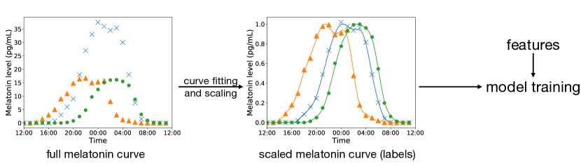
(a)

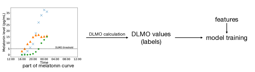
(b)

Figure 1. A comparison of model training pipelines between previous methods that use frequently sampled data and our method. (a) The pipeline of existing methods that train a model for estimating melatonin level. The method requires fitting and scaling the melatonin curve first, which requires complete melatonin curves. (b) The pipeline of our method that trains a model for estimating the dim-light melatonin onset (DLMO) directly. Different colors denote melatonin profiles of different people. Our method does not require collecting a full melatonin profile.

In addition to the above mentioned drawbacks, the previous DLMO modeling methods based on frequently sampled sensor data (Kolodyazhniy et al., 2011, 2012; Gil et al., 2013; Stone et al., 2019) are designed for estimating melatonin concentrations first, and DLMO values are then calculated based on the predicted melatonin curve. The pipeline of these methods is shown in Figure 1(a). Since there is a wide inter-individual variation in the peak value of DLMO (Burgess and Fogg, 2008), these methods need to fit and scale the melatonin curves, which requires the full melatonin profile. This training approach of DLMO that requires the entire melatonin profile (rather than only DLMO), however, greatly increases the cost and participant burdens of melatonin collection because 1) the participants must remain awake for many hours after their habitual bedtime to collect samples and 2) processing and assaying the samples to obtain melatonin measurement is expensive.

In light of these limitations from previous methods, we propose a two-step framework for estimating DLMO using the data from two time scales. In the first step, the framework summarizes all features prior to the day of interest. The second step combines the result of the first step and the current day’s frequently sampled data to estimate DLMO. For the implementation, we evaluate three moving average models to summarize sleep onset/offset time for the first step. For the second step, we apply recurrent neural network (RNN) methods to predict DLMO.

The main contributions of this paper are:

1. We construct a two-step framework for estimating DLMO using features of two time scales: both daily sampled data and frequently sampled data. This is a generalization of all current models.

2. To implement the framework, we compare three moving average models for the daily sampled data, and evaluate them for extracting features from the daily sleep timing data.

3. To the best of our knowledge, this work is the first to predict DLMO directly using frequently sampled data (using the pipeline in Figure 1(b)), which requires less data collection for training the model.

4. We show that the model using features of two time scales is significantly better than the one using only one type of feature.

2. Data Preparation

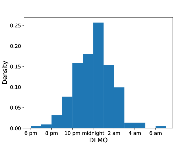
Figure 2. The distribution of DLMO values in our dataset. The mean DLMO value is 23.43$\pm$1.76.

The data were collected in the SNAPSHOT (Sleep, Networks, Affect, Performance, Stress, and Health using Objective Techniques) study, including approximately 1-3 months of daily physiological and behavioral data and one to three DLMO laboratory assessments from 207 undergraduate college students from 2013 to 2017 (Sano, 2016; Phillips et al., 2017; McHill et al., 2017; Taylor et al., 2017; Sano et al., 2018b, a). Participants in the 2017 cohort had DLMO calculated one to three times over $\sim$3 months of data collection; all other participants have only one DLMO assessment in $\sim$1 month of data collection. We split the data by using the data collected during 2013-2016 ($\sim$1 month of data) as the training set and the data collected in the 2017 cohort ($\sim$3 months of data) as the test set. There are 192 training samples and 31 test samples. Participants were recruited through email.

2.1. DLMO

The melatonin concentrations were assayed from saliva collected every hour from 3 pm to 7 am under dim-light conditions ($<$4 lux) (McHill et al., 2017). The environment was sound-attenuated and temperature-controlled. Participants were permitted to take brief naps between samples and interact with other participants, but were not allowed to use any electronic devices due to the light emitted by such devices (Chang et al., 2015). Food that might influence the concentration of melatonin in saliva was not allowed during this time. They were also instructed to avoid eating or drinking and to maintain stable posture, for the 20 min prior to each sample. DLMO was determined by linear interpolation of the time that melatonin values first exceeded a threshold of 5 pg/mL (Phillips et al., 2017). The distribution of DLMO values collected in our dataset is shown in Figure 2. The mean DLMO value is 23.43$\pm$1.76.

2.2. Physiological and Behavioral Data

During the experiments, the participants wore (i) a wrist sensor on their dominant hand (Q-sensor, Affectiva, USA) to continuously measure ST and three-axis AC at 8Hz sampling rate, and (ii) a wrist actigraphy monitor on their non-dominant hand (Motion Logger, AMI, USA) to measure LE stored at 1 minute intervals. We logarithmically transformed the LE values and computed the L2-norm for AC. We segmented the data into one-hour bins and computed the mean values over each hour as the features of that hour. Sleep onset/offset times were computed based on sleep diary queries every morning and Motion Logger data analyzed using Action-4 software (Sano et al., 2018a). For any missing data of each feature, we used linear interpolation to impute the data for missing data less than 12 hours, which performs the best for our dataset with other imputation methods (data not shown). We did not use data sets that contain missing segments longer than 12 hours for the day prior to DLMO collection. After those data sets were removed, the longest missing segment was about 8 hours.

2.3. Removing the Effect of Daylight-Saving Time

Since some participants were studied during the clock shift between standard time and daylight saving time, we subtracted one hour from the clock time during daylight-saving time to make clock times uniform across all participants. This standardization is essential for the following reasons:

1. Our target is to design a model that predicts DLMO tracking the user activity. A time in our dataset is a feature (sleep time) or a label (DLMO). By standardizing the times, the model does not need to assess whether the clock time is changed.

2. If the clock time changes, user activity would also change due to social constraints. The standardization of time clock allows the model to capture this adjustment, which could provide better prediction performance intuitively.

3. Some participants in our dataset experienced the clock time change while some did not. This standardization makes the model perform consistently for both groups of participants.

3. Methods

We represent human circadian phase by the following formula

(1) $$\phi_{t}=f(\psi_{t-1},x_{t})$$

where $\phi_{t}$ is the circadian phase (e.g., DLMO) on day $t$, $\psi_{t-1}$ is the extracted features from the data prior to the day $t$, $x_{t}$ is the 24-hour frequently sampled data starting from the wake-up time of the $t$ th day, and $f(\cdot,\cdot)$ is the model that combines all features for estimating $\phi_{t}$. Previous studies have described this relationship mathematically when $x_{t}$ is LE or sleep timing data, and $\psi_{t-1}:=\phi_{t-1}$ (Kronauer et al., 1999; Hilaire et al., 2007b). In practice, the true value of $\phi_{t-1}$ is never known. In this section, we introduce our methods of estimating DLMO under this framework. Since we are only interested in estimating the DLMO values on a specific day, $t$ in Formula 1 is constant, thus, we rewrite this formula as follows.

(2) $$\phi=f(\psi,x)$$

The framework is composed of the following two steps:

1. Extracting features from the data prior to the current day, (i.e., calculating $\psi$).

2. Estimating DLMO with $\psi$ and current day’s frequently sampled data $x$ (e.g., LE, ST, and AC) (i.e., modeling $f$).

It should be noted that while $x$ only consists of frequently sampled data of the current day, $\psi$ can be derived from both daily sampled data and frequently sampled data before the current day. This framework is the extension of the models that use only one type of time-scale data.

• For models only using daily sleep onset/offset times (Martin and Eastman, 2002; Burgess and Eastman, 2005), $\phi=\psi$ where $\psi$ is the features derived by the daily data.

• For models only using frequently sampled data of the current day (Kolodyazhniy et al., 2011; Gil et al., 2013; Stone et al., 2019; Kolodyazhniy et al., 2012), $\phi=f(0,x)$.

3.1. Our Implementation of the Two-Step Framework

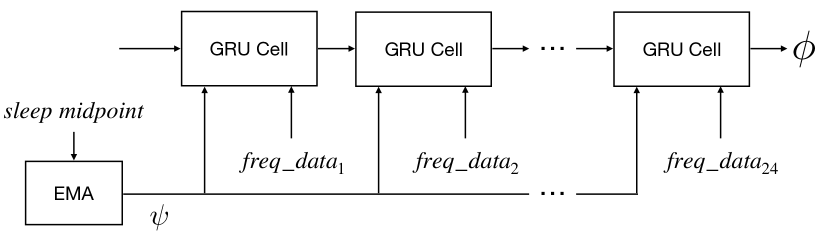
Figure 3. The structure of RNN${}_{\text{EMA}}$ as an example of our framework. In this model, we first use an exponential moving average (EMA) model for calculating $\psi$ from 7-day daily sleep parameters. Then we feed the hourly frequently sampled features (”freq_data”) of light exposure, skin temperature, physical activity, and the output of the EMA model into different RNN cell (gated recurrent unit (GRU) in our implementation) for calculating current day’s DLMO $\phi$.

In the first step of the model, we use daily sleep midpoint (i.e., midpoint between sleep onset and sleep offset times) during the past week for deriving $\psi$, and define $\psi$ as an estimator of $\phi$. This definition allows $\psi$ to be a bridge between daily sleep timing parameters and $\phi$. The sleep midpoint of the $i$th day over the past $n$ days is denoted as $T_{i}$. In this work, we set $n=7$. The first model we evaluate is a simple moving average (SMA) model which was used in (Martin and Eastman, 2002; Burgess and Eastman, 2005; Crowley et al., 2006):

(3) $$\psi_{\text{SMA}} =a\sum_{i=1}^{n}T_{i}+b$$

where $a$ and $b$ are trainable parameters, and are trained by least squares.

The second model for evaluating $\psi$ is an exponential moving average (EMA) model. The model can be presented as

(4) $$\psi_{\text{EMA}} =a\sum_{i=1}^{n}\alpha^{n-i}T_{i}+b$$

where $a$ and $b$ are trainable parameters, and $\alpha$ is a fixed decay rate. We choose 0.9 as the value of $\alpha$ as we found this value was the best parameter for modeling $\phi$ in our preliminary experiments (data not shown).

We also introduce a moving average model (MA, a more generalized model) for comparison:

$$\psi_{\text{MA}}=\sum_{i=1}^{n}w_{i}T_{i}+b$$

where $w_{i}$ and $b$ are trainable parameters.

For the second step of the model, we apply a recurrent neural network (RNN) for estimating $\phi$. RNN models have shown great success in natural language processing and sequence learning (Haykin, 1994; Mikolov et al., 2010). For the $i$th cell, time, $\psi$ and the frequently sampled data $x$ (i.e., LE, wrist ST, and AC) of the $i$th hour on that day are used as the inputs. We input $\psi$ to each cell because the timing of light stimuli impacts the direction and magnitude of the circadian phase shift (Khalsa et al., 2003). In our implementation, we use gated recurrent unit (GRU) cells for the RNN model because they have better performance on small datasets (Chung et al., 2014). As an example, our structure of RNN${}_{\text{EMA}}$ that uses EMA in the first step is shown in Figure 3.

The training process contains three independent steps. First, we use least squares to train the model that uses sleep midpoints. Then, we fix the parameters in this model and train an RNN. Lastly, we fine-tune all trainable parameters in the model using back-propagation.

3.2. Comparison of Moving Average Models

SMA v.s. EMA

We consider the following two averages of the sleep midpoint time

$$\overline{T}_{t}^{\text{SMA}}=\frac{\sum\limits_{i=0}^{n-1}T_{t-i}}{n}$$

$$\overline{T}_{t}^{\text{EMA}}=\frac{\sum\limits_{i=0}^{n-1}\alpha^{i}T_{t-i}}{\sum\limits_{i=0}^{n-1}\alpha^{i}}$$

Here $\overline{T}_{t}^{\text{SMA}}$ represents a simple moving average and $\overline{T}_{t}^{\text{EMA}}$ is an exponential moving average. Suppose $T_{i}$ follows a Gaussian channel:

$$T_{i}=\widetilde{T}_{i}+\varepsilon_{i}$$

where $\widetilde{T}_{i}$ is the true value of sleep midpoint with i.i.d. noise $\varepsilon_{i}\sim\mathcal{N}(0,\sigma^{2})$. Therefore,

$$\overline{T}_{t}^{\text{SMA}}\sim\mathcal{N}\left(\frac{\sum\limits_{i=0}^{n-1}\widetilde{T}_{t-i}}{n},\frac{\sigma^{2}}{n}\right)$$

$$\overline{T}_{t}^{\text{EMA}}\sim\mathcal{N}\left(\frac{\sum\limits_{i=0}^{n-1}\alpha^{i}\widetilde{T}_{t-i}}{\sum\limits_{i=0}^{n-1}\alpha^{i}},\frac{\sum\limits_{i=0}^{n-1}\alpha^{2i}}{\left(\sum\limits_{i=0}^{n-1}\alpha^{i}\right)^{2}}\sigma^{2}\right)$$

According to Cauchy-Schwarz inequality, $\left(\sum\limits_{i=0}^{n-1}\alpha^{i}\right)^{2}\leq n\sum\limits_{i=0}^{n-1}\alpha^{2i}$. $\overline{T}_{t}^{\text{EMA}}$ has a larger variance than $\overline{T}_{t}^{\text{SMA}}$. When $\sigma$ is large (data are noisy), the average value of the sleep midpoint is a better approach for reducing the noise.
Intuitively, $\overline{T}_{t}^{\text{EMA}}$ is a more reliable feature for estimating DLMO because recent sleep timing would be expected to be more highly correlated with DLMO than distant sleep timing as sleep gates the light exposure that might shift DLMO (Czeisler and Buxton, 2017). In addition, sleep timing of each day is highly influenced by circadian phase of that day as human circadian rhythm strongly regulates human sleep timing (Mistlberger, 2005; Czeisler and Buxton, 2017). Therefore, we hypothesize that the EMA model is more sensitive to noise, and it could be a better method for estimating DLMO when the noise is small.

SMA/EMA v.s. MA

MA is an extension of SMA/EMA with more tuneable parameters. Therefore, more data are required for training MA. Green (1991) suggests a sample size of $N\geq 50+8m$ for the multiple regression where $m$ is the number of predictor variables.

4. Experiments

For the two-step model we designed, we tested three questions:

1. In the first step, which moving average model performs the best for estimating DLMO?

2. Does the two-step model perform better for estimating DLMO than models that only use either daily sampled or frequently sampled data?

3. Which combination of frequently sampled data (ST, AC, and LE) performs the best for estimating DLMO? Fewer types of data reduce the cost of required sensors.

We designed three experiments to address these three questions. The code was implemented in Python and the machine learning framework we used was PyTorch (Paszke et al., 2019).

4.1. Question 1: Comparison among Moving Average Models

We first compare the performance of three moving average models: SMA, EMA and MA.

1. We calculated three values for comparing performance:

   • RMSE${}_{\text{all}}$: We calculate the root-mean-square error (RMSE) using all data for training the linear regression model.

   • RMSE${}_{\text{val}}$: We evaluate the model’s generalization ability for avoiding overfitting problems, by calculating RMSE on a leave-one participant-out cross-validation data set.

   • $<$1h: We calculate the percentage of the test samples with absolute error of less than one hour using a leave-one participant-out cross-validation data set. Similar metrics are also reported in (Burgess and Eastman, 2005; Phillips et al., 2017).

2. We evaluated the effect of statistical noise in the data on the SMA, EMA, and MA models by adding Gaussian noise with standard deviation $\sigma$ to each value of the sleep midpoint. For each $\sigma$, we repeatedly generated noisy sleep data and calculated the coefficient of determination ($r^{2}$) between true DLMO and the predicted DLMO using noisy sleep data 20,000 times.

3. We also tested model performance with different window sizes between 3 and 8 days (i.e., the number of days of data in the model).

4.2. Question 2: Performance of the Two-Step Model

Based on the first experiment, we choose the best moving average model $M$ for implementing a two-step model. We compare the performance of the model $M$, the corresponding two-step model RNN_M, and the RNN model with 24-hour frequently sampled data RNN${}_{\text{24-hour}}$. Here we do not leverage more than 24 hours of frequently sampled data because previous work (Kolodyazhniy et al., 2011) reports that 24-hour data is better than longer data sets for predicting DLMO, and longer data set are more likely to contain longer missing data segments. In our dataset, at least 25% of 7-day (168-hour) frequently sampled data contain missing segments longer than 12 hours. The removal of the missing segments leaves smaller amounts of data to analyze, and makes it harder to compare the results from the model with 7-day frequently sampled data with other models.

We use the following metrics to compare the three models.

• RMSE${}_{\text{val}}$: To reduce the computation cost of evaluating the model, we run 10-fold cross-validation instead of leave-one-out cross-validation on the training set to get the hyperparameters with the lowest RMSE. We define the RMSE value of the $i$th validation set as $r_{i}$, we define RMSE over all validation sets as RMSE${}_{\text{val}}=\sqrt{\frac{r_{1}^{2}+r_{2}^{2}+\cdots+r_{10}^{2}}{10}}$.

• RMSE${}_{\text{test}}$: After selecting the best hyper-parameters based on RMSE${}_{\text{val}}$ and training the model using all training samples, we calculate the RMSE value on the test set.

• $<$1h: We calculate the percentage of the test samples with absolute error of less than one hour.

4.3. Question 3: Comparison among Different Input Combinations

To address the third question, we compare the models with different combinations of frequently sampled data. For the best model $M$ in the first experiment (Section 4.1), we replace its frequently sampled data with one type of input or arbitrary two-type-of-input combination. A one-input model with LE, ST or AC is denoted as RNN${}_{M}^{\text{(LE)}}$, RNN${}_{M}^{\text{(ST)}}$ and RNN${}_{M}^{\text{(AC)}}$ respectively. Similarly, we define the models with two types of input as RNN${}_{M}^{\text{(LE, ST)}}$, RNN${}_{M}^{\text{(LE, AC)}}$ and RNN${}_{M}^{\text{(ST,AC)}}$. We use the same metrics as in Section 4.2.

We use cross validation and Akaike Information Criterion (AIC) at the same time for selecting the best combination of features because all criteria for feature selection from high-dimensional and small sample data have drawbacks. For example, (i) small bias exists in selecting features using cross-validation when the feature number is small compared with data size (Smialowski et al., 2009). Note that cross validation is always a biased estimate for feature selection as the feature selection process requires accessing test data (Refaeilzadeh et al., 2007). (ii) AIC is an information theory-based metric that considers the performance of the model and the number of parameters in the model. Note that there are many assumptions and approximations in AIC (Davies et al., 2005), and the degrees of freedom (DOF) in neural networks are generally much less than the number of parameters (Murata et al., 1994; Gao and Jojic, 2016). For our RNN work, DOF has not yet been studied. (iii) Information theory-based feature selection methods cannot be applied in our dataset because our dataset is not large enough for estimating the mutual information between each high dimensional feature and the DLMO value.

5. Results

5.1. Question 1: Comparison among Moving Average Models

The three moving average models perform similarly on the validation sets ($p=0.97$, repeated measures ANOVA) (Table 1). For the model performance of moving average models after adding noise (Figure 4), the $r^{2}$ values followed Gaussian distribution for each $\sigma$ value ($p<0.002$, D’Agostino’s $K$ test). The MA model showed the highest $r^{2}$ between DLMO and sleep data (Figure 4). When the level of noise was low, the features extracted by the EMA model showed larger $r^{2}$ than SMA. With increased noise, all models performed worse. SMA performed slightly better than EMA when $\sigma>2$. When $\sigma=2$, there was no significant difference between the $r^{2}$ of SMA and EMA ($p=1.0$, two-sample t-tests with Bonferroni correction). For other $\sigma$s the differences were significant ($p<0.001$, statistically but there differences may not be important in practice.).

There was no significant difference for each model by different data window sizes ($n$ in the moving average models) ($p>0.05$, within-group multiple paired comparison).

Table 1. A comparison among 3 moving average models.

Model	RMSE${}_{\text{all}}$	RMSE${}_{\text{val}}$	$<$1h
SMA	1.36	1.38	56.5%
EMA	1.36	1.37	56.9%
MA	1.33	1.38	56.8%

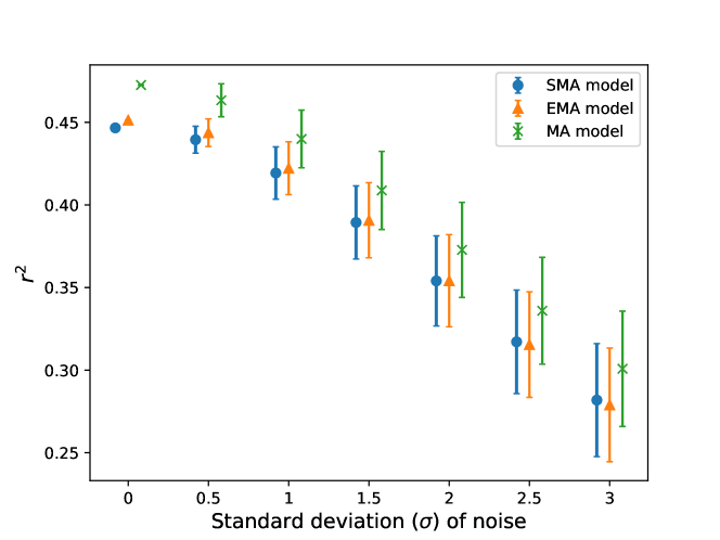
Figure 4. The performance of each moving average model with different different standard deviation of noise.

5.2. Question 2: Performance of the Two-Step Model

Since all three moving average models performed similarly (Section 5.1), we implemented RNN${}_{\text{SMA}}$ (RMSE${}_{\text{val}}$=1.25, RMSE${}_{\text{test}}$=1.34, $<$1h: 61.3%), RNN${}_{\text{EMA}}$ (RMSE${}_{\text{val}}$=1.21, RMSE${}_{\text{test}}$=1.38, $<$1h: 64.5%), and RNN${}_{\text{MA}}$ (RMSE${}_{\text{val}}$=1.26, RMSE${}_{\text{test}}$=1.36, $<$1h: 48.4%). The training time for the cross validation sets was about 30 minutes on a CPU (2.6 GHz Intel Core i7). The difference among these models on validation sets was not significant ($p=0.66$, repeated measures ANOVA). Therefore, in the next step, we used the model RNN${}_{\text{EMA}}$ because it had the best score on two of the three metrics (i.e., RMSE${}_{\text{val}}$ and $<$1h).

Table 2 shows that RNN${}_{\text{EMA}}$ showed the lowest RMSE${}_{\text{val}}$ and RMSE${}_{\text{test}}$ and highest $<$1h. The model performance for EMA, RNN${}_{\text{24-hour}}$, and RNN${}_{\text{EMA}}$ on the validation sets (RMSE${}_{\text{val}}$) was significantly different ($p=0.0022$, repeated measures ANOVA). RNN${}_{\text{EMA}}$ performed significantly better than the other two models (for RNN${}_{\text{EMA}}$ v.s. EMA, $p=0.048$; for RNN${}_{\text{EMA}}$ v.s. RNN${}_{\text{24-hour}}$, $p=0.013$, using multiple paired t-test with Bonferroni correction). Therefore, the combination of 7-day daily sampled data and 24-hour frequently sampled data (RNN${}_{\text{EMA}}$) showed statistically significantly better model performance than EMA or RNN${}_{\text{24-hour}}$ (Figure 5). Note that while the RMSE varied across each validation set, the RMSE for RNN${}_{\text{EMA}}$ was lowest in 9/10 sets.

Table 2. A comparison among three different structures.

Model	RMSE${}_{\text{val}}$	RMSE${}_{\text{test}}$	$<$1h
EMA	1.38	1.42	54.8%
RNN${}_{\text{24-hour}}$	1.51	1.55	41.9%
RNN${}_{\text{EMA}}$	1.21	1.38	64.5%

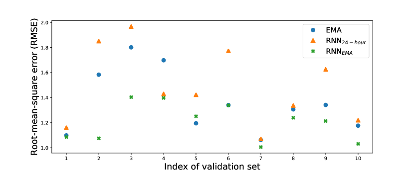
Figure 5. The root-mean-square error of each validation set for the three models.

5.3. Question 3: Comparison among Different Input Combinations

Table 3. A comparison among models with different input.

	Model	RMSE${}_{\text{val}}$	RMSE${}_{\text{test}}$	$<$1h	AIC
	RNN${}_{\text{EMA}}$	1.21	1.38	64.5%	207.6
	RNN${}_{\text{EMA}}^{\text{(LE)}}$	1.31	1.44	61.3%	247.3
	RNN${}_{\text{EMA}}^{\text{(ST)}}$	1.27	1.48	45.2%	216.6
	RNN${}_{\text{EMA}}^{\text{(AC)}}$	1.33	1.46	48.4%	280.2
	RNN${}_{\text{EMA}}^{\text{(LE, ST)}}$	1.29	1.36	61.3%	220.4
	RNN${}_{\text{EMA}}^{\text{(LE, AC)}}$	1.29	1.39	54.8%	231.5
	RNN${}_{\text{EMA}}^{\text{(ST, AC)}}$	1.26	1.38	48.4%	210.5

There was no statistically significant difference among the RMSE${}_{\text{val}}$ values of the models with different feature combinations ($p=0.119$, repeated measures ANOVA) (Table 3). The model using all features performed the best based on $<$1h and AIC. RNN${}_{\text{EMA}}^{\text{(LE, ST)}}$ would be another good options for those who want to reduce the number of sensors based on RMSE${}_{\text{test}}$ and $<$1h.

5.4. Error Analysis

For the relationship between the predicted DLMO of our EMA and RNN${}_{\text{EMA}}$ models and true DLMO value for the test data (Figure 6), the Pearson correlation of the prediction errors (i.e., absolute different between predicted DLMO and true DLMO) of two models was 0.596 with $p=4.0\times 10^{-4}$, which suggests a strong correlation between the errors. Visual inspection shows that the model tends to predict later DLMO if the experimental DLMO is prior to midnight, and predict earlier DLMO if the experimental DLMO is after midnight.

To understand how to improve EMA model, we studied whether missing patterns in sleep parameters and sleep regularity of a participant influence the performance of the model. We first split the data into two categories based on whether the absolute error is less than 1 hour or not. Then, we used Mann-Whitney U test to compare the missingness/sleep regularity in these two categories. There were no statistically significant relationships in (i) the relationship between the number of missing values in the sleep parameters and DLMO prediction errors of EMA and (ii) the relationship between standard deviations of sleep parameters across days (i.e., sleep regularity) and DLMO prediction errors of EMA.

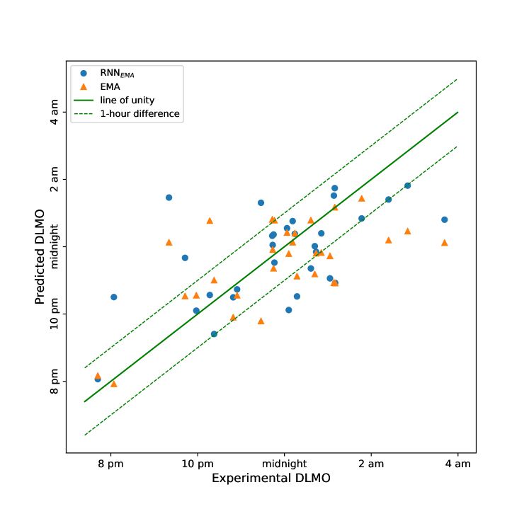
Figure 6. The relationship between the predicted DLMO values from two methods and the experimental DLMO.

6. Discussion

6.1. Choice of Moving Average Models

Previous work that analyzed the relationship between sleep data and DLMO value (Martin and Eastman, 2002; Burgess and Eastman, 2005; Crowley et al., 2006) used only SMA models. In this paper, we compared SMA with the other two moving average models.

SMA v.s. EMA

In Section 3.2, we hypothesized that the EMA model is more sensitive to noise but its performance is better when the noise is limited. Our experiment supported this (Figure 4): EMA performs better than SMA when the noise is small ($\sigma<2$) but it is worse when the noise is large ($\sigma>2$). With the development of technologies that reduce noise, an EMA model could be more useful in the future.

SMA/EMA v.s. MA

In this work, we collected 223 samples. According to the analysis in Section 3.2, the sample size was large enough, but the prediction performance of MA was similar to that of SMA/EMA. As a result, MA was not preferred for predicting DLMO using sleep midpoints.

6.2. The Performance of the Proposed Two-Step Models

Table 4. A comparison between RNN${}_{\text{EMA}}$ and previous work using a subset of the data in this datasets. For the values that are not reported, we use the symbol ’/’.

Model	RMSE${}_{\text{val}}$	RMSE${}_{\text{test}}$	$<$1h
RNN${}_{\text{EMA}}$	1.21	1.38	64.5%
Neural Network (Brown et al., 2018)	1.45	1.49	/
Limit Cycle Oscillator (Phillips et al., 2017)	/	/	43%

In this paper, we proposed a two-step framework using two time-scale features for estimating DLMO. Our experiment showed that the performance of the two-step models was significantly better than the models using only daily sampled or frequently sampled data. We also compare our model with other work (Phillips et al., 2017; Brown et al., 2018) using a subset of the data in this datasets (Table 4). Our model performed better on the $<$1h metric (65% v.s. 43%) than a limit cycle oscillator based method with light input (Phillips et al., 2017). The performance of our model was also better than that of a neural network method (Brown et al., 2018) that used sleep timing, frequently sampled sensor data (LE and AC) and demographic information (gender, personality types and sleep quality index) as input features (RMSE${}_{\text{val}}$: 1.21 v.s. 1.45, RMSE${}_{\text{test}}$: 1.38 v.s. 1.49). Neither of those publications included the other metrics.

The error analysis showed that the error of our RNN${}_{\text{EMA}}$ model was strongly correlated with the error of EMA. Therefore, one approach to improve RNN${}_{\text{EMA}}$ is to improve the accuracy of the moving average model.

This novel framework is the generalization of current models that leverage both daily sampled data and frequently sampled data. The model proposed in this paper may be eventually useful for estimating DLMO as a marker of human circadian phase. Every feature we used in our model is derived from wearable sensors that are low-cost, easy to use, and can provide data in close to real time. As noted above, some existing methods (Kolodyazhniy et al., 2011, 2012; Gil et al., 2013; Stone et al., 2019) were designed for estimating melatonin instead of predicting DLMO directly. These existing methods therefore require a complete melatonin profile (e.g., the shortest length of data was 22-hour long in these reports (Gil et al., 2013)) for scaling the melatonin amount when training the model, which is expensive and inconvenient. The model proposed in the work directly estimates DLMO and requires much less melatonin collection for training the model.

The ideas of this work can be applied to other regression or classification tasks with sensor data with different sample rates. In this work, we have two different time scales of data: the daily sampled data capture behavioral or physiological parameters from each day, and the frequently sampled data are stored minute by minute. Other times scales of data can be also investigated.

6.3. Limitation and Future Work

There are some limitations in our work. First, we did not compare this model with previous work (Kolodyazhniy et al., 2011, 2012; Gil et al., 2013; Stone et al., 2019) because those works developed models to estimate the amount of melatonin first and then derived DLMO based on the estimated melatonin profile, which required normalizing the melatonin data by fitting the curve using sufficient melatonin data. Since our melatonin was sampled from 13 hours long laboratory studies, it was not sufficient for fitting the curve. We leave this comparison to future work and we will also explore whether we can train a better model using all melatonin data, not just DLMO.

Second, the dataset we used were collected from students at a single college. The relationship of the parameters may be different in other groups of people. The models need to be tested in other populations for confirming the generalizability. We will further evaluate the performance of our models on other populations such as shift workers, people with jet lag, and people with psychiatric disorders to explore clinical application of our model.

Third, we explored the best feature combination for estimating DLMO. Our current result (Table 3) was not conclusive, as different metrics in our experiment produced different results for different feature combinations. The comparison of feature combination has to be further investigated with a larger dataset.

As additional future work, we will explore whether the model can be improved by utilizing other features including phone screen time and caffeine intake, which also affect human circadian phase (Cajochen et al., 2011; Burke et al., 2015), as well as specifics of physical/mental condition. Non-linear models will be examined for sleep parameters, and we will compare this framework with other existing approaches. Potential applications using sensor-based DLMO estimation include adjusting the timing of drug administration and designing better work schedules for each individual based on their circadian phase; these and other applications requiring knowledge of circadian phase will be more feasible once non-invasive inexpensive long-term monitoring methods are available.

7. Conclusion

In this paper, we proposed and evaluated a two-step framework that leverages features of two time scales for predicting DLMO. This framework is the extension of previously used models with input of either frequently sampled data (i.e., light exposure, skin temperature, physical activity) or daily sampled data (i.e., sleep onset/offset timing). The experiment showed that the proposed model performed better than the model only using one-time-scale feature.

- (1)
- Baron and Reid (2014) Kelly Glazer Baron and Kathryn J. Reid. 2014. Circadian misalignment and health. International Review of Psychiatry 26, 2 (2014), 139–154.
- Benloucif et al. (2008) Susan Benloucif, Helen J. Burgess, Elizabeth B. Klerman, Alfred J. Lewy, Benita Middleton, Patricia J. Murphy, Barbara L. Parry, and Victoria L. Revell. 2008. Measuring melatonin in humans. Journal of Clinical Sleep Medicine 4, 01 (2008), 66–69.
- Bonmati-Carrion et al. (2014) Maria A. Bonmati-Carrion, Benita Middleton, Victoria L. Revell, Debra J. Skene, Angeles Rol, and Juan A. Madrid. 2014. Circadian phase asessment by ambulatory monitoring in humans: Correlation with dim light melatonin onset. Chronobiology International 31, 1 (2014), 37–51.
- Brown et al. (2018) Lindsey S. Brown, Melissa A. St. Hilaire, Andrew W. McHill, Andrew J. K. Phillips, Laura K. Barger, Akane Sano, Rosalind W. Picard, Elizabeth B. Klerman, and Francis J. Doyle III. 2018. A neural network predicts human circadian phase from non-invasive, short-timeframe actigraphy and demographic data: A step towards automated control of circadian phase. (2018). Poster presented at 2018 Society for Research on Biological Rhythms.
- Burgess and Eastman (2005) Helen J. Burgess and Charmane I. Eastman. 2005. The dim light melatonin onset following fixed and free sleep schedules. Journal of Sleep Research 14, 3 (2005), 229–237.
- Burgess and Fogg (2008) Helen J Burgess and Louis F Fogg. 2008. Individual differences in the amount and timing of salivary melatonin secretion. PloS ONE 3, 8 (2008).
- Burke et al. (2015) Tina M. Burke, Rachel R. Markwald, Andrew W. McHill, Evan D. Chinoy, Jesse A. Snider, Sara C. Bessman, Christopher M. Jung, John S. O’Neill, and Kenneth P. Wright. 2015. Effects of caffeine on the human circadian clock in vivo and in vitro. Science Translational Medicine 7, 305 (2015), 305ra146–305ra146.
- Cajochen et al. (2011) Christian Cajochen, Sylvia Frey, Doreen Anders, Jakub Späti, Matthias Bues, Achim Pross, Ralph Mager, Anna Wirz-Justice, and Oliver Stefani. 2011. Evening exposure to a light emitting diodes (LED)-backlit computer screen affects circadian physiology and cognitive performance. American Journal of Physiology-Heart and Circulatory Physiology (2011).
- Chang et al. (2015) Anne-Marie Chang, Daniel Aeschbach, Jeanne F Duffy, and Charles A Czeisler. 2015. Evening use of light-emitting eReaders negatively affects sleep, circadian timing, and next-morning alertness. Proceedings of the National Academy of Sciences 112, 4 (2015), 1232–1237.
- Chung et al. (2014) Junyoung Chung, Caglar Gulcehre, KyungHyun Cho, and Yoshua Bengio. 2014. Empirical evaluation of gated recurrent neural networks on sequence modeling. arXiv preprint arXiv:1412.3555 (2014).
- Crowley et al. (2006) Stephanie J. Crowley, Christine Acebo, Gahan Fallone, and Mary A. Carskadon. 2006. Estimating dim light melatonin onset (DLMO) phase in adolescents using summer or school-year sleep/wake schedules. Sleep 29, 12 (2006), 1632–1641.
- Czeisler and Buxton (2017) Charles A. Czeisler and Orfeu M. Buxton. 2017. The human circadian timing system and sleep-wake regulation. In Principles and Practice of Sleep Medicine: Sixth Edition. Elsevier Inc., 362–376.
- Czeisler et al. (1990) Charles A. Czeisler, Michael P. Johnson, Jeanne F. Duffy, Emery N. Brown, Joseph M. Ronda, and Richard E. Kronauer. 1990. Exposure to bright light and darkness to treat physiologic maladaptation to night work. New England Journal of Medicine 322, 18 (1990), 1253–1259.
- Davies et al. (2005) Simon L. Davies, Andrew A. Neath, and Joseph E. Cavanaugh. 2005. Cross validation model selection criteria for linear regression based on the Kullback–Leibler discrepancy. Statistical Methodology 2, 4 (2005), 249–266.
- Di Lorenzo et al. (2003) Luigi Di Lorenzo, Giovanni De Pergola, Carlo Zocchetti, Nicola L’Abbate, Antonella Basso, Nicola Pannacciulli, Mauro Cignarelli, Riccardo Giorgino, and Leonardo Soleo. 2003. Effect of shift work on body mass index: results of a study performed in 319 glucose-tolerant men working in a Southern Italian industry. International Journal of Obesity 27, 11 (2003), 1353.
- Gao and Jojic (2016) Tianxiang Gao and Vladimir Jojic. 2016. Degrees of freedom in deep neural networks. arXiv preprint arXiv:1603.09260 (2016).
- Gil et al. (2013) Enrique A. Gil, Xavier L. Aubert, Els I. S. Møst, and Domien G. M. Beersma. 2013. Human circadian phase estimation from signals collected in ambulatory conditions using an autoregressive model. Journal of Biological Rhythms 28, 2 (2013), 152–163.
- Green (1991) Samuel B. Green. 1991. How many subjects does it take to do a regression analysis. Multivariate Behavioral Research 26, 3 (1991), 499–510.
- Haykin (1994) Simon Haykin. 1994. Neural networks. Vol. 2. Prentice Hall New York.
- Hilaire et al. (2007a) Melissa A. St. Hilaire, Claude Gronfier, Jamie M. Zeitzer, and Elizabeth B. Klerman. 2007a. A physiologically based mathematical model of melatonin including ocular light suppression and interactions with the circadian pacemaker. Journal of Pineal Research 43, 3 (2007), 294–304.
- Hilaire et al. (2007b) Melissa A. St. Hilaire, Elizabeth B. Klerman, Sat Bir S. Khalsa, Kenneth P. Wright Jr., Charles A. Czeisler, and Richard E. Kronauer. 2007b. Addition of a non-photic component to a light-based mathematical model of the human circadian pacemaker. Journal of Theoretical Biology 247, 4 (2007), 583–599.
- Khalsa et al. (2003) Sat Bir S Khalsa, Megan E Jewett, Christian Cajochen, and Charles A Czeisler. 2003. A phase response curve to single bright light pulses in human subjects. The Journal of Physiology 549, 3 (2003), 945–952.
- Klerman et al. (2002) Elizabeth B. Klerman, Hayley B. Gershengorn, Jeanne F. Duffy, and Richard E. Kronauer. 2002. Comparisons of the variability of three markers of the human circadian pacemaker. Journal of Biological Rhythms 17, 2 (2002), 181–193.
- Kolodyazhniy et al. (2011) Vitaliy Kolodyazhniy, Jakub Späti, Sylvia Frey, Thomas Götz, Anna Wirz-Justice, Kurt Kräuchi, Christian Cajochen, and Frank H. Wilhelm. 2011. Estimation of human circadian phase via a multi-channel ambulatory monitoring system and a multiple regression model. Journal of Biological Rhythms 26, 1 (2011), 55–67.
- Kolodyazhniy et al. (2012) Vitaliy Kolodyazhniy, Jakub Späti, Sylvia Frey, Thomas Götz, Anna Wirz-Justice, Kurt Kräuchi, Christian Cajochen, and Frank H. Wilhelm. 2012. An improved method for estimating human circadian phase derived from multichannel ambulatory monitoring and artificial neural networks. Chronobiology International 29, 8 (2012), 1078–1097.
- Kronauer et al. (1999) Richard E. Kronauer, Daniel B. Forger, and Megan E. Jewett. 1999. Quantifying human circadian pacemaker response to brief, extended, and repeated light stimuli over the phototopic range. Journal of Biological Rhythms 14, 6 (1999), 501–516.
- Martin and Eastman (2002) Stacia K. Martin and Charmane I. Eastman. 2002. Sleep logs of young adults with self-selected sleep times predict the dim light melatonin onset. Chronobiology International 19, 4 (2002), 695–707.
- McHill et al. (2017) Andrew W. McHill, Andrew J. K. Phillips, Charles A. Czeisler, Leigh Keating, Karen Yee, Laura K. Barger, Marta Garaulet, Frank A. J. L. Scheer, and Elizabeth B. Klerman. 2017. Later circadian timing of food intake is associated with increased body fat. The American Journal of Clinical Nutrition 106, 5 (2017), 1213–1219.
- Mikolov et al. (2010) Tomáš Mikolov, Martin Karafiát, Lukáš Burget, Jan Černockỳ, and Sanjeev Khudanpur. 2010. Recurrent neural network based language model. In Eleventh Annual Conference of the International Speech Communication Association.
- Mistlberger (2005) Ralph E. Mistlberger. 2005. Circadian regulation of sleep in mammals: role of the suprachiasmatic nucleus. Brain Research Reviews 49, 3 (2005), 429–454.
- Morris et al. (2016) Christopher J. Morris, Taylor E. Purvis, Kun Hu, and Frank A. J. L. Scheer. 2016. Circadian misalignment increases cardiovascular disease risk factors in humans. Proceedings of the National Academy of Sciences 113, 10 (2016), E1402–E1411.
- Murata et al. (1994) Noboru Murata, Shuji Yoshizawa, and Shun-ichi Amari. 1994. Network information criterion-determining the number of hidden units for an artificial neural network model. IEEE Transactions on Neural Networks 5, 6 (1994), 865–872.
- Pandi-Perumal et al. (2007) Seithikurippu R. Pandi-Perumal, Marcel Smits, Warren Spence, Venkataramanujan Srinivasan, Daniel P. Cardinali, Alan D. Lowe, and Leonid Kayumov. 2007. Dim light melatonin onset (DLMO): a tool for the analysis of circadian phase in human sleep and chronobiological disorders. Progress in Neuro-Psychopharmacology and Biological Psychiatry 31, 1 (2007), 1–11.
- Paszke et al. (2019) Adam Paszke, Sam Gross, Francisco Massa, Adam Lerer, James Bradbury, Gregory Chanan, Trevor Killeen, Zeming Lin, Natalia Gimelshein, Luca Antiga, Alban Desmaison, Andreas Kopf, Edward Yang, Zachary DeVito, Martin Raison, Alykhan Tejani, Sasank Chilamkurthy, Benoit Steiner, Lu Fang, Junjie Bai, and Soumith Chintala. 2019. PyTorch: An Imperative Style, High-Performance Deep Learning Library. In Advances in Neural Information Processing Systems 32, H. Wallach, H. Larochelle, A. Beygelzimer, F. d'Alché-Buc, E. Fox, and R. Garnett (Eds.). Curran Associates, Inc., 8024–8035. http://papers.neurips.cc/paper/9015-pytorch-an-imperative-style-high-performance-deep-learning-library.pdf
- Phillips et al. (2017) Andrew J. K. Phillips, William M. Clerx, Conor S. O’Brien, Akane Sano, Laura K. Barger, Rosalind W. Picard, Steven W. Lockley, Elizabeth B. Klerman, and Charles A. Czeisler. 2017. Irregular sleep/wake patterns are associated with poorer academic performance and delayed circadian and sleep/wake timing. Scientific Reports 7, 1 (2017), 3216.
- Refaeilzadeh et al. (2007) Payam Refaeilzadeh, Lei Tang, and Huan Liu. 2007. On comparison of feature selection algorithms. In Proceedings of AAAI Workshop on Evaluation Methods for Machine Learning II, Vol. 3. 5.
- Rusak and Zucker (1979) Benjamin Rusak and Irving Zucker. 1979. Neural regulation of circadian rhythms. Physiological Reviews 59, 3 (1979), 449–526.
- Sack et al. (2007) Robert L. Sack, Dennis Auckley, R. Robert Auger, Mary A. Carskadon, Kenneth P. Wright Jr., Michael V. Vitiello, and Irina V. Zhdanova. 2007. Circadian rhythm sleep disorders: part I, basic principles, shift work and jet lag disorders. Sleep 30, 11 (2007), 1460–1483.
- Sano (2016) Akane Sano. 2016. Measuring college students’ sleep, stress, mental health and wellbeing with wearable sensors and mobile phones. Ph.D. Dissertation. Massachusetts Institute of Technology.
- Sano et al. (2018a) Akane Sano, Weixuan Chen, Daniel Lopez-Martinez, Sara Taylor, and Rosalind W. Picard. 2018a. Multimodal Ambulatory Sleep Detection Using LSTM Recurrent Neural Networks. IEEE Journal of Biomedical and Health Informatics (2018).
- Sano et al. (2018b) Akane Sano, Sara Taylor, Andrew W. McHill, Andrew J. K. Phillips, Laura K. Barger, Elizabeth B. Klerman, and Rosalind Picard. 2018b. Identifying objective physiological markers and modifiable behaviors for self-reported stress and mental health status using wearable sensors and mobile phones: Observational study. Journal of Medical Internet Research 20, 6 (2018), e210.
- Smialowski et al. (2009) Pawel Smialowski, Dmitrij Frishman, and Stefan Kramer. 2009. Pitfalls of supervised feature selection. Bioinformatics 26, 3 (2009), 440–443.
- Stone et al. (2019) Julia E. Stone, Andrew J. K. Phillips, Suzanne Ftouni, Michelle Magee, Mark Howard, Steven W. Lockley, Tracey L. Sletten, Clare Anderson, Shantha M. W. Rajaratnam, and Svetlana Postnova. 2019. Generalizability of A neural network Model for circadian phase prediction in Real-World conditions. Scientific Reports 9, 1 (2019), 1–17.
- Taylor et al. (2017) Sara Ann Taylor, Natasha Jaques, Ehimwenma Nosakhare, Akane Sano, and Rosalind W. Picard. 2017. Personalized Multitask Learning for Predicting Tomorrow’s Mood, Stress, and Health. IEEE Transactions on Affective Computing (2017).